improving crosshole radar velocity tomograms: a new ... · improving crosshole radar velocity...
TRANSCRIPT
IA
J
psneacotEamCi�i
z
©
GEOPHYSICS, VOL. 72, NO. 4 �JULY-AUGUST 2007�; P. J31–J41, 12 FIGS.10.1190/1.2742813
mproving crosshole radar velocity tomograms:new approach to incorporating high-angle traveltime data
ames D. Irving1, Michael D. Knoll2, and Rosemary J. Knight3
tsaawtimitoBos
ABSTRACT
To obtain the highest-resolution ray-based tomographic imag-es from crosshole ground-penetrating radar �GPR� data, wide an-gular ray coverage of the region between the two boreholes is re-quired. Unfortunately, at borehole spacings on the order of a fewmeters, high-angle traveltime data �i.e., traveltime data corre-sponding to transmitter-receiver angles greater than approxi-mately 50° from the horizontal� are notoriously difficult to incor-porate into crosshole GPR inversions. This is because �1� lowsignal-to-noise ratios make the accurate picking of first-arrivaltimes at high angles extremely difficult, and �2� significant to-mographic artifacts commonly appear when high- and low-angleray data are inverted together. We address and overcome these
INTRODUCTIONnpa
ccAhpmbhwb
w
20, 200ifornia;
o; preseail: rk
J31
wo issues for a crosshole GPR data example collected at the Boi-e Hydrogeophysical Research Site �BHRS�. To estimate first-rrival times on noisy, high-angle gathers, we develop a robustnd automatic picking strategy based on crosscorrelations,here reference waveforms are determined from the data
hrough the stacking of common-ray-angle gathers. To overcomencompatibility issues between high- and low-angle data, we
odify the standard tomographic inversion strategy to estimate,n addition to subsurface velocities, parameters that describe araveltime ‘correction curve’ as a function of angle. Applicationf our modified inversion strategy, to both synthetic data and theHRS data set, shows that it allows the successful incorporationf all available traveltime data to obtain significantly improvedubsurface velocity images.
Crosshole ground-penetrating radar �GPR� traveltime tomogra-hy is a popular geophysical method for high-resolution imaging ofubsurface electromagnetic �EM� wave velocity. With this tech-ique, a short EM pulse is radiated from a transmitter antenna, locat-d in one borehole, and recorded at a receiver antenna, located in andjacent borehole. The first-break traveltimes of energy for variousonfigurations of the two antennas are then picked and inverted tobtain an image �tomogram� of the distribution of velocity betweenhe boreholes. Because of the strong contrast that exists between theM-wave velocity of water �0.03 m/ns� and that of dry earth materi-ls ��0.15 m/ns�, the velocities obtained with crosshole GPR to-ography are highly correlated with water content in the subsurface.onsequently, the technique is very useful for detecting differences
n porosity in the saturated zone, and changes in soil water retentionoften linked to changes in grain size� in the vadose zone. Of interestn our research is the use of such information in the development of
Manuscript received by the Editor February 1, 2007; published online June1Formerly Stanford University, Department of Geophysics, Stanford, Cal
erland. E-mail: [email protected] Boise State University, Department of Geosciences, Boise, Idah3Stanford University, Department of Geophysics, Stanford, California. E-m2007 Society of Exploration Geophysicists.All rights reserved.
umerical models for groundwater flow and contaminant trans-ort. Resolution of crosshole GPR tomograms is critical for thispplication.
In environmental applications, crosshole GPR tomography isommonly performed between boreholes that are spaced quitelosely together �on the order of a few meters� �e.g., Peterson, 2001;lumbaugh and Chang, 2002; Tronicke et al., 2002b�. At such bore-ole spacings, the potential exists in theory for excellent tomogra-hic resolution. This is because, even for the relatively shallow ��20� borehole depths typical of environmental applications, close
orehole spacings allow for wide angular coverage of the inter-bore-ole region, which is a key requirement for high-resolution imagingith ray-based tomography �e.g., Menke, 1984; Rector and Wash-ourne, 1994�.
In practice, however, two significant problems are encounteredhen attempting to take advantage of this wide angular coverage.
7.presently University of Lausanne, Institute of Geophysics, Lausanne, Swit-
ntly Boise, Idaho. E-mail: [email protected]@pangea.stanford.edu.
Fea�apatecwsbibrG2azeer
tlodcaldifm�t
sseaBmdawiKtlr�
eod
hdcewb2nmldawtmTtr
sswmttatssfs
BefaassppdcrfittmaHotasw
J32 Irving et al.
irst, the arrival times of energy traveling at high transmitter-receiv-r angles �commonly, angles greater than �50° from the horizontal�re often very difficult to pick because of low signal-to-noise ratiosS/N� in the data. This results not only because of an increasedmount of attenuation at high angles arising from longer travelaths, but also because of the radiation patterns of the crosshole GPRntennas, which decrease to zero amplitude along the end-fire direc-ions �e.g., Peterson, 2001; Holliger and Bergmann, 2002�. Second,ven when high-angle traveltimes can be determined reliably atlose borehole spacings, difficulties are commonly encounteredhen attempting to incorporate these data into crosshole GPR inver-
ions. Specifically, the high-angle data often appear to be incompati-le with the lower-angle data available, and cause significant numer-cal artifacts in the resulting tomograms �Peterson, 2001; Alum-augh and Chang, 2002; Irving and Knight, 2005a�. As a result, cur-ent practice is to exclude high-angle traveltime data from crossholePR inversions �e.g., Alumbaugh and Chang, 2002; Linde et al.,006�. This has the advantage of allowing reasonable subsurface im-ges to be obtained. However, it comes at the cost of reduced hori-ontal resolution; high-angle data are necessary to constrain the lat-ral variability of the subsurface velocity field. Depending on thend use of the crosshole GPR images, this reduction in horizontalesolution may be a serious drawback.
In this paper, we present a case study attempting to address �ratherhan avoid� the above two issues for a crosshole GPR data set col-ected at the Boise Hydrogeophysical Research Site �BHRS�. Tovercome the high-angle picking problem, we develop a strategy foretermining first-break times from crosshole GPR data using cross-orrelations. With this technique, picking of the example data set isccomplished automatically and reliably, even for traces with veryow S/N corresponding to high transmitter/receiver angles. To ad-ress the high-angle incompatibility problem at close borehole spac-ngs, we first discuss what we believe to be the cause of this problemor the BHRS data set. Using this information, we then develop aodified inversion strategy that allows all available traveltimes
both high- and low-angle� to be incorporated successfully into theomographic reconstruction.
FIELD SITE AND DATA DESCRIPTION
The BHRS is a research wellfield located near Boise, Idaho in ahallow, unconfined aquifer �Barrash et al., 1999�. The aquifer con-ists of an approximately 18-m-thick layer of coarse, unconsolidat-d, braided-stream deposits �gravels and cobbles with sand lenses�,nd is underlain by clay and basalt. The purpose of developing theHRS was to create a site for testing geophysical and hydrologicethods, with the goal of using these methods to characterize the
istribution of hydrogeological properties in heterogeneous alluvialquifers. Eighteen wells have been emplaced at the site, all of whichere carefully completed to minimize disturbance of the surround-
ng formation and cased with 4-in PVC well screen �Barrash andnoll, 1998�. For additional information about the BHRS, including
he different stratigraphic units that have been identified using well-og, core, and geophysical data, see Barrash and Clemo �2002�, Bar-ash and Reboulet �2004�, Tronicke et al. �2004�, Clement et al.2006�, Clement and Barrash �2006�, and Moret et al. �2006�.
The crosshole GPR field data analyzed in this study were collect-d at the BHRS between wells labeledA1 and B2 during the summerf 1999. These two wells are approximately 3.5 m apart and 20 meep. The Malå RAMAC/GPR borehole antennas used for the cross-
ole survey had a specified center frequency of 250 MHz. To con-uct the survey, common-receiver gathers were collected. The re-eiver antenna, located in well B2, was lowered every 0.2 m. Forach receiver location, the transmitter antenna �located in well A1�as fired approximately every 0.05 m as it was lowered down theorehole. The resulting crosshole GPR data set contained over5,000 traces. Because much of this information is redundant andot necessary to obtain the highest-possible-resolution ray-based to-ographic image, we considered data from every fourth transmitter
ocation in our analysis. Subsampling in this manner made theepth-sampling intervals in the transmitter and receiver boreholespproximately equal. In addition, we considered only those traceshere both the transmitter and receiver antenna elements were con-
ained entirely below the water table �determined using a water leveleter to be at approximately 3 m depth at the time of the survey�.he final data set analyzed, representative of the saturated zone be-
ween 3.6 and 18.2 m depth, contained 5329 traces with transmitter/eceiver angles ranging from �75° to �75° from the horizontal.
To account for borehole deviations in our analysis — a criticaltep in crosshole GPR tomography, especially at close boreholepacings �Peterson, 2001� — borehole trajectories in the subsurfaceere measured carefully using a magnetic deviation logging tool. Toinimize deviations of the transmitter and receiver locations from
he tomographic plane, we applied a very slight coordinate rotationo the data such that, in the new coordinate system, all borehole devi-tions were constrained to within 3 cm of this plane. Parameters forhe rotation were determined using an inversion that minimized theum of the squared out-of-plane deviations. Finally, the GPR systemampling frequency and transmitter fire time were determined care-ully before the survey by firing the antennas in air in a walkawayurvey using a calibrated survey tape.
CROSSCORRELATION PICKINGOF TRAVELTIMES
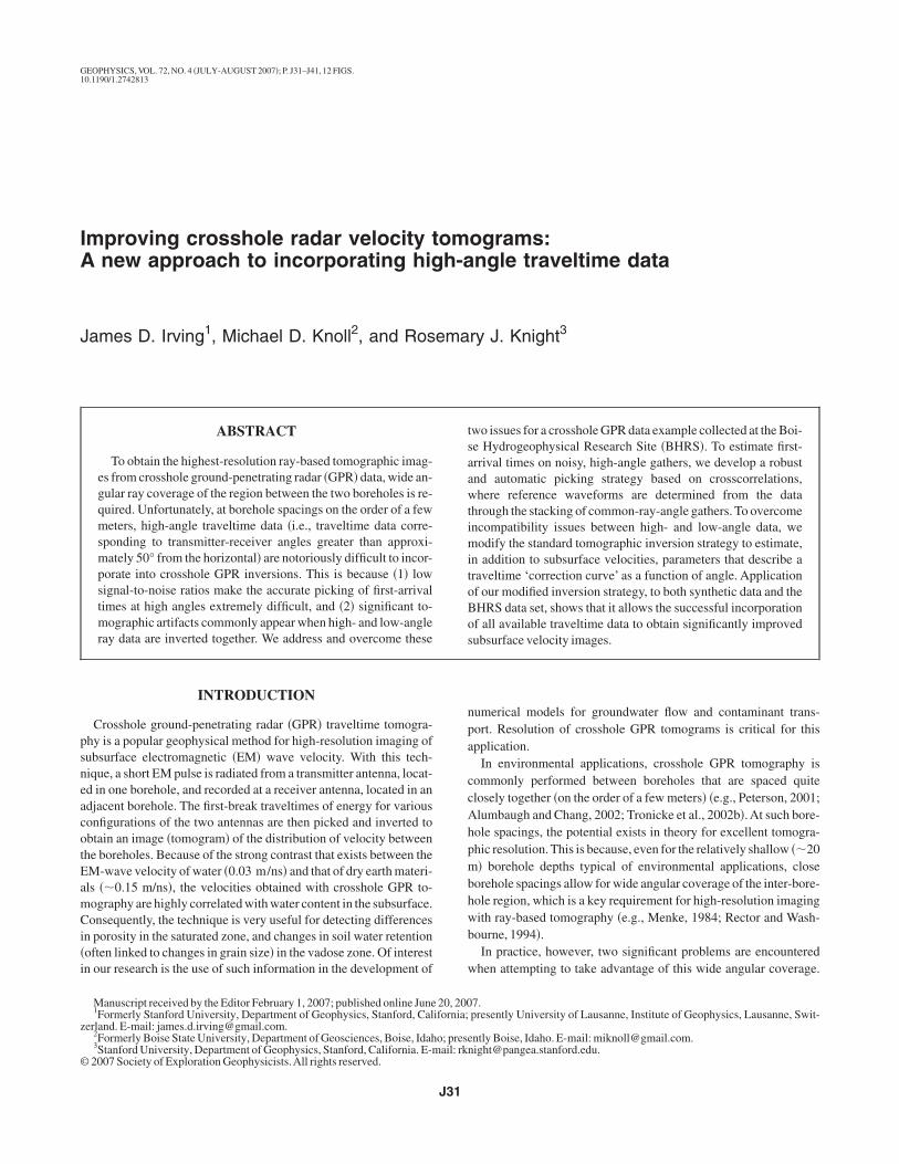
Figure 1 shows an example common-receiver gather from theHRS data set, corresponding to a receiver depth of 5.33 m.All trac-s in the gather have been normalized by their maximum amplitudesor easier comparison. The figure clearly illustrates why difficultiesre often encountered when attempting to pick first breaks in high-ngle crosshole GPR data. Notice that when the antenna depths areimilar �near the top of the plot�, the recorded waveforms have a verytrong S/N and picking of first breaks is straightforward; on the up-ermost trace, the first break occurs just before the small positiveeak located at approximately 55 ns. However, as the transmitterepth �and thus the angle between antennas� increases, the S/N de-reases to the point where, near the bottom of Figure 1, the first-ar-iving peak cannot even be seen, let alone picked.Although low-passltering may be of some help in attempting to pick such noisy traces,
he large amount of filtering required for traces with very low S/N of-en can affect significantly the apparent onset of signal.Another idea
ight be to pick the point of maximum amplitude on the noisy tracesnd then back off a prescribed amount to obtain the first breaks.owever, such picking is not robust. More importantly, the positionf the first break with respect to the trace maximum will vary withransmitter/receiver angle because the GPR waveform changes withngle. Clearly, signal is present in the lower traces of Figure 1; its on-et is simply overshadowed by noise. The question is: Can we find aay to use what signal is there to estimate the first arrivals?
ea�Wttatm
btsfdmttrfiewhep
ia�nedcta1
atft
rtcttwticpu
thtbcarav
Fteh F
Incorporating high-angle traveltime data J33
One solution for the robust estimation of traveltimes in the pres-nce of significant noise, that has been used widely in earthquakend exploration seismic studies, is the crosscorrelation techniquee.g., Peraldi and Clement, 1972; VanDecar and Crosson, 1990;
oodward and Masters, 1991; Molyneux and Schmitt, 1999�. Withhis method, the discrete crosscorrelation of a trace and a high-quali-y reference waveform �having a known arrival time� is determined,nd then the difference in traveltime between the two signals is ob-ained from the time shift at which the crosscorrelation value is a
aximum.Ideally, the reference waveform used with this technique should
e noise-free and have the same shape as the waveform present onhe trace in question. Although synthetics are often used to obtainuch a waveform in earthquake studies, we obtained reference wave-orms for crosscorrelation picking of the BHRS data set from theata themselves. We found that synthetic modeling required toouch knowledge about GPR system, antenna, and earth parameters
o yield waveforms that were sufficiently close enough to those inhe field data for effective crosscorrelation analysis. To obtain theeference waveforms, we stack traces that have been aligned on therst arrival. Because the GPR pulse changes with transmitter/receiv-r angle �a result of variations in antenna radiation and receptionith angle, and likely also propagation dispersion along travel pathsaving different lengths�, we determine a number of different refer-nce waveforms that represent ranges in angle where the arrivingulses have similar shape.
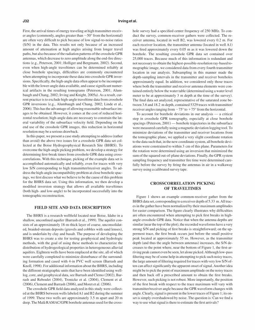
Figure 2 is a flowchart illustrating the sequence of steps involvedn our crosscorrelation picking procedure. The crosshole GPR datare first preprocessed by removing any DC offset from each tracedetermined from the mean value of the trace before the onset of sig-al� and by normalizing each trace by the signal maximum �estimat-d by low-pass filtering the data and finding the maximum value�. Ifesired, extremely noisy traces with no apparent signal can be dis-arded straightaway to reduce the number of bad picks obtained withhe technique. Next, the crosshole data are sorted into common-ray-ngle gathers �e.g., Pratt and Worthington, 1988; Pratt and Goulty,991; Tronicke et al., 2002a�. To do this, we create a set of angle bins
40 60 80 100 120 140 160 180 200
4
6
8
10
12
14
16
18
Tra
nsm
itter
dep
th (
m)
Time (ns)
igure 1. Common-receiver gather from the BHRS data set showinghe difficulties in picking first-break times at high transmitter-receiv-r angles arising from low S/N. Receiver depth is 5.33 m. All tracesave been normalized by their maximum values.
nd place each trace into the appropriate bin based on the transmit-er/receiver angle. To determine a high-quality reference waveformor each angle bin, the waveforms in each gather must be aligned andhen stacked.
Because aligning the traces requires some means of estimating theelative time shifts between the waveforms, we use crosscorrela-ions, but in an iterative manner as follows: Initially, the traces in aommon-ray-angle gather are aligned by crosscorrelating them withhe trace in the gather having the highest S/N. This places the majori-y of traces into proper alignment, which allows for a higher qualityaveform to be obtained through stacking. In the second iteration,
races in the gather are aligned again, but this time by crosscorrelat-ng them with the mean trace from the previous iteration. This pro-ess can be continued until the vast majority of traces in a gather areroperly aligned; however, we have found that two iterations aresually sufficient.
Once the reference waveforms for each angle range have been de-ermined, their first arrivals are picked manually. The entire cross-ole data set is then picked automatically by crosscorrelating eachrace with the appropriate reference waveform. To increase the ro-ustness of this algorithm, we limit the number of lags used in therosscorrelations to reasonable values �i.e., for the BHRS data set,bsolute differences in arrival time between individual traces and theeference trace were assumed to be less than 20 ns�. As a final step,ll of the automatic picks made with this method should be checkedisually for accuracy. Bad picks are generally quite obvious, as they
Data preprocessing1) remove DC shift from each trace
2) normalize each trace by signal maximum3) discard data where signal is clearly absent
Sort data into common-ray-angle gathers
Determine mean trace for each angle gather
Pick first-arrival time on each mean trace
Manually inspect the picks
Done
Crosscorrelate each trace in data set withappropriate reference waveform for that angle,
and use to determine first-arrival time
Another iteration needed to properly align traces
in each gather?
Yes
No
Align traces in each common-ray-anglegather by crosscorrelating with either:
1) trace having highest signal-to-noise ratio2) mean trace from previous iteration
igure 2. Flowchart of our crosscorrelation picking procedure.

tt
griacesnusSpfibf
mhc�
co
gcfcfi
Bmosctoo
wtsatspetiHcttpsto
a
F6t
Ftam
a
c
FsPrd
J34 Irving et al.
end to be caused by the crosscorrelation being maximized when thewo signals are mismatched by a full cycle.
As an example, Figure 3a shows one of the common-ray-angleathers obtained from the BHRS data set for the 65° to 70° angleange. Here, the transmitter/receiver angle is measured from the hor-zontal with positive angles representing the case where the receiverntenna is located above the transmitter antenna. Two iterations ofrosscorrelating were used to align the traces in this high-angle gath-r. The waveforms in the gather are clearly visible and have veryimilar shapes, but they are contaminated by significant amounts ofoise which makes picking the first breaks extremely difficult. Fig-re 3b, on the other hand, shows the mean trace that was obtained bytacking the 322 traces in Figure 3a together. Here, we see that the/N has been greatly increased and that a small, positive, first-arrivaleak, not clearly visible on any individual trace, is now easily identi-ed. The much higher S/N of this mean trace, and the fact that its firstreak can be picked easily, make it an excellent reference waveformor crosscorrelation analysis.
Figure 4 shows the mean traces that were obtained in the aboveanner for each angle group in the BHRS data set. The waveforms
ave been aligned on their manually picked first arrivals for easieromparison. Angle bins were created for every 5° increment from75° to �75°, which yielded 30 reference waveforms. Figure 4
learly shows why we must determine these waveforms as a functionf angle when picking crosshole GPR data, as opposed to using a sin-
0 50 100 150 200 250 300
80
100
120
140
160
180
200
Tim
e (n
s)
−1 0 Amplitude Trace number
1
80
100
120
140
160
180
200
) b)
igure 3. �a� Common-ray-angle gather and �b� mean trace for the5° to 70° angle range in the BHRS data set. The picked first-arrivalime on the mean trace is indicated with a horizontal dashed line.
•80 −60 −40 −20 0 20 40 60 80
0
20
40
60
80
Angle bin center (°)
Tim
e (n
s)
igure 4. Mean traces determined for the BHRS data set by stackinghe different common-ray-angle gathers. The traces have beenligned at t = 0 on their picked first arrivals and normalized by theiraximum values.
le reference waveform for the entire data set; there is a significanthange in shape of the GPR pulse with angle that must be accountedor. Also notice that all of the reference waveforms in Figure 4, in-luding the ones on both ends if scaled enough in amplitude, haverst-arrival times that are easily identified.Finally, Figure 5 shows four example receiver gathers from the
HRS data set upon which the first-break times, all determined auto-atically with our technique, have been superimposed in red. In all
f the gathers, the picks are seen to be very reasonable. This is de-pite the fact that significant noise is present at high transmitter/re-eiver angles, and in many cases, the positive first-arrival peak athese angles cannot be visually identified. We conclude that pickingf the BHRS data using crosscorrelations was a very effective meansf determining first-arrival times.
In using crosscorrelations to pick first breaks as described above,e implicitly assume that waveforms recorded at similar transmit-
er/receiver angles have similar shapes, and are thus suitable fortacking to obtain useful, high-quality reference waveforms. Thisssumption is valid only in the absence of very sharp velocity con-rasts in the subsurface, as such velocity contrasts can give rise totrongly scattered arrivals that interfere with the direct-arrivingulse. Indeed, the BHRS data shown in Figures 3–5 were collectedntirely below the water table and were void of any strongly scat-ered arrivals, as evidenced by the similarity of direct-arriving pulsesn each angle gather and the success of the crosscorrelation picking.ad the survey region spanned the water table �a very large velocity
ontrast� or had the antenna positions been nearer to the very reflec-ive air/earth boundary, problems could have been encountered withhe picking of some traces. It may be possible to overcome suchroblems �and thus extend the technique to data sets with significantcattering� through a modification of the algorithm, or by filteringhe data beforehand to remove the scattered arrivals. This is a topicf future research.
Time (ns)
Tra
nsm
itter
dep
th (
m)
50 100 150 200
5
10
15
)
Time (ns)
Tra
nsm
itter
dep
th (
m)
50 100 150 200
5
10
15
b)
Time (ns)
Tra
nsm
itter
dep
th (
m)
50 100 150 200
5
10
15
)
Time (ns)
Tra
nsm
itter
dep
th (
m)
50 100 150 200
5
10
15
d)
igure 5. Four common-receiver gathers from the BHRS data sethowing the results of our crosscorrelation picking procedure.icked first breaks are shown in red; �a� receiver depth = 5.33 m; �b�eceiver depth = 8.73 m; �c� receiver depth = 12.33 m; �d� receiverepth = 15.53 m.
ibpcwGisedfcawtsdr
hPibhbbpetamrFogioF
acthl
ctidtvgsmatws
tcgdu�tm0nna
s
F
a
c
Fpa=m
Incorporating high-angle traveltime data J35
INCOMPATIBILITY OF HIGH-ANGLE DATA
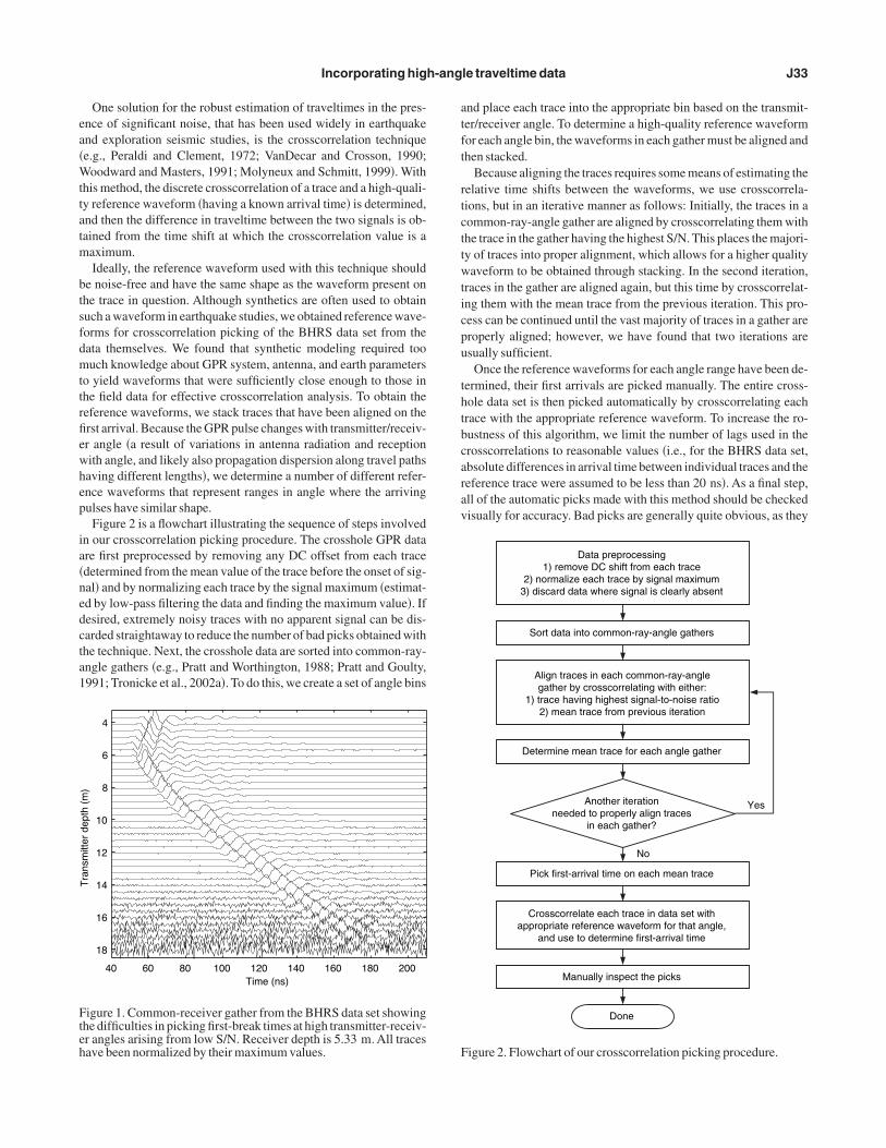
Next we address the second problem encountered when attempt-ng to take advantage of the wide angular coverage provided by closeorehole spacings: the fact that high-angle traveltime data often ap-ear to be incompatible with lower-angle data. Significant insightan be gained into this problem through velocity-versus-angle plots,here the average velocity calculated along each ray in a crossholePR data set �assuming a straight path between the antenna centers�
s plotted as a function of the transmitter/receiver angle. Figure 6hows such a scatter plot for the BHRS data set. The figure was creat-d using the picks obtained with the crosscorrelation technique justescribed. Notice the general trend that exists in velocity with angleor these data; the along-the-ray velocities at high transmitter/re-eiver angles are markedly greater than those determined for lowerngles. This trend clearly illustrates why problems are encounteredhen high- and low-angle traveltimes are inverted together; the two
ypes of data are providing inconsistent information about the sub-urface velocity field. Reasonable subsurface velocity models �thato not possess significant amounts of anisotropy� should not giveise to large-scale trends in velocity with angle.
We have found that the trend seen in Figure 6 is typical of cross-ole GPR data collected between closely spaced boreholes �see alsoeterson, 2001�.Although Peterson �2001� suspects that such a trend
s caused by refracted waves that travel partly through air-filledoreholes and arrive before the direct pulse, the BHRS data shownere were collected between water-filled wells where this should note a problem. It is also very difficult to explain the trend in Figure 6y the other factors discussed in Peterson �2001� that can cause ap-arent variations in velocity with angle in crosshole GPR data. Forxample, although errors in the calculation of the transmitter fireime and inaccurate borehole location measurements could result inplot resembling Figure 6, every step was taken to ensure that theseeasurements were accurate for the BHRS data set. Also, such er-
ors do not explain the consistency we have observed in the trend inigure 6 across different data sets. In addition, although the presencef anisotropy can give rise to general trends in velocity with angle,eologically reasonable anisotropy �i.e., due to thin horizontal layer-ng� results in velocities that are greater at low angles, which is thepposite of what we observe. Finally, it is unlikely that the trend inigure 6 is the simple result of having less-accurate traveltime picks
−50 0 50
Tx-Rx angle (°)
Ave
rage
vel
ocity
alo
ng th
e ra
y (m
/ns)
0.092
0.090
0.088
0.086
0.084
0.082
0.080
0.078
igure 6. Velocity-versus-angle plot for the BHRS data set.
t high transmitter/receiver angles because of decreased S/N. In thatase, one would not expect picks to be consistently earlier than therue first-arrival times �which is required to yield higher velocities atigh angles�. The question, then, is why do we have this trend in ve-ocity with angle for the BHRS data set?
Recently, Irving and Knight �2005a� addressed the high-angle in-ompatibility issue in crosshole GPR tomography, and suggestedhat the problem may result from a common assumption made dur-ng the inversion of the data: that first-arriving energy always travelsirectly between the antenna centers. They proposed that, at highransmitter/receiver angles, first-arriving energy may actually travelia the antenna tips. This will be possible when the velocity of ener-y traveling along the antennas vant is greater than the velocity of theubsurface medium between the boreholes vmed. Using numericalodeling and considering a number of different borehole diameters
nd external medium properties, Irving and Knight �2005a� showedhat often vant will be significantly greater than vmed, in both air- andater-filled boreholes, for a common commercial GPR antenna de-
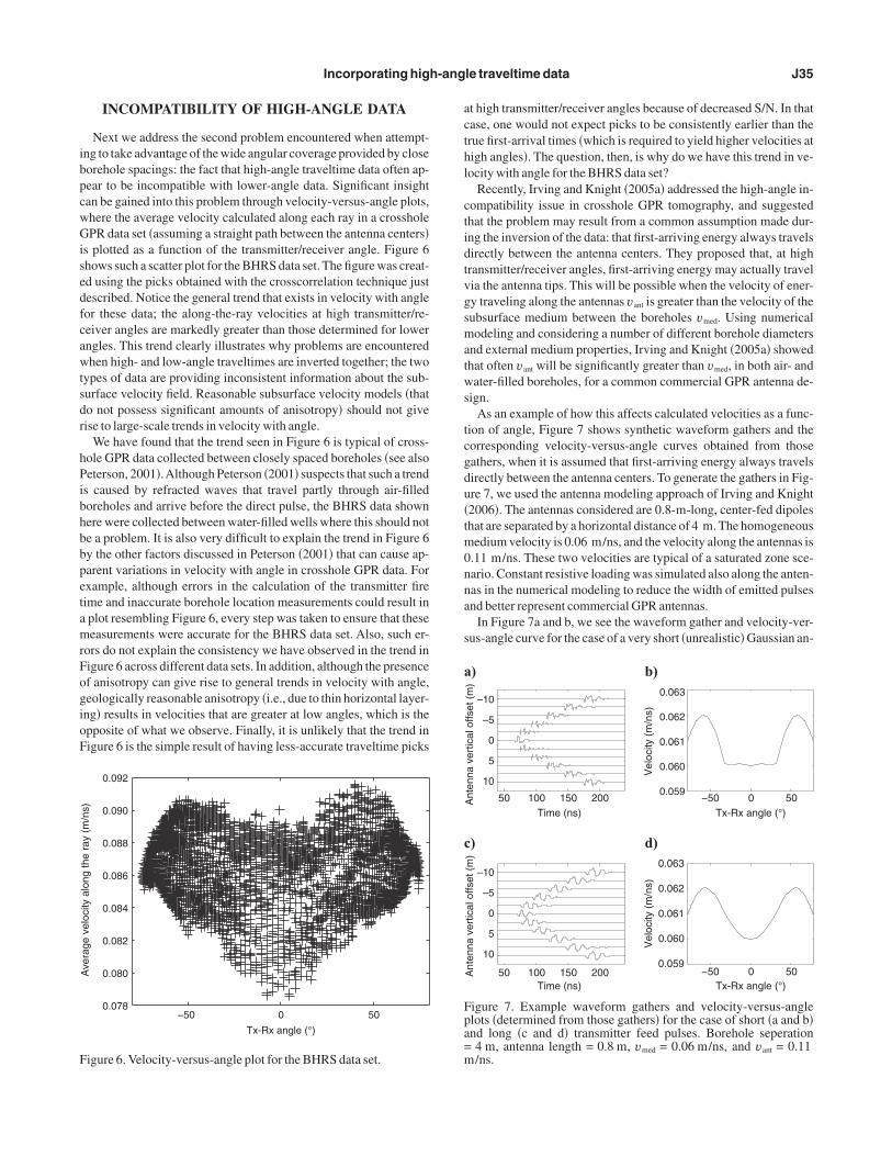
ign.As an example of how this affects calculated velocities as a func-
ion of angle, Figure 7 shows synthetic waveform gathers and theorresponding velocity-versus-angle curves obtained from thoseathers, when it is assumed that first-arriving energy always travelsirectly between the antenna centers. To generate the gathers in Fig-re 7, we used the antenna modeling approach of Irving and Knight2006�. The antennas considered are 0.8-m-long, center-fed dipoleshat are separated by a horizontal distance of 4 m. The homogeneous
edium velocity is 0.06 m/ns, and the velocity along the antennas is.11 m/ns. These two velocities are typical of a saturated zone sce-ario. Constant resistive loading was simulated also along the anten-as in the numerical modeling to reduce the width of emitted pulsesnd better represent commercial GPR antennas.
In Figure 7a and b, we see the waveform gather and velocity-ver-us-angle curve for the case of a very short �unrealistic� Gaussian an-
50 100 150 200 Ant
enna
ver
tical
offs
et (
m)
Time (ns)
50 100 150 200
−50 0 50 Tx-Rx angle (°)
Time (ns) Tx-Rx angle (°)
Vel
ocity
(m
/ns)
V
eloc
ity (
m/n
s)
−50 0 50 0.059
0.060
0.061
0.062
0.063
–10
–5
0
5
10
0.063
0.062
0.061
0.060
0.059
–10
–5
0
5
10
) b)
Ant
enna
ver
tical
offs
et (
m)
) d)
igure 7. Example waveform gathers and velocity-versus-anglelots �determined from those gathers� for the case of short �a and b�nd long �c and d� transmitter feed pulses. Borehole seperation4 m, antenna length = 0.8 m, vmed = 0.06 m/ns, and vant = 0.11/ns.
tnrIael0acwtunGtrsW
vGIgsnbpdlsl
wabrclewpmamcwhseIrshcvi
tgne
pi
wtstttasm
wtop2oe
lt1txawnctabawdtea
dlitwcasvaw
J36 Irving et al.
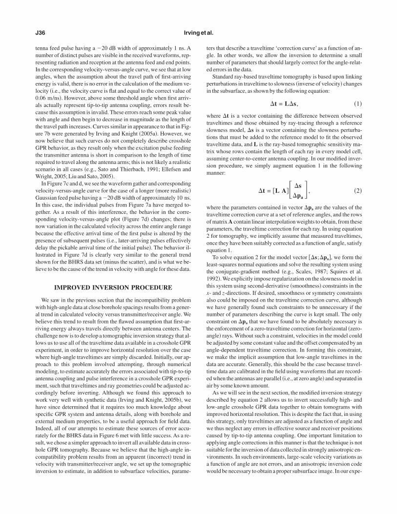
enna feed pulse having a �20 dB width of approximately 1 ns. Aumber of distinct pulses are visible in the received waveforms, rep-esenting radiation and reception at the antenna feed and end points.n the corresponding velocity-versus-angle curve, we see that at lowngles, when the assumption about the travel path of first-arrivingnergy is valid, there is no error in the calculation of the medium ve-ocity �i.e., the velocity curve is flat and equal to the correct value of.06 m/ns�. However, above some threshold angle when first arriv-ls actually represent tip-to-tip antenna coupling, errors result be-ause this assumption is invalid. These errors reach some peak valueith angle and then begin to decrease in magnitude as the length of
he travel path increases. Curves similar in appearance to that in Fig-re 7b were generated by Irving and Knight �2005a�. However, weow believe that such curves do not completely describe crossholePR behavior, as they result only when the excitation pulse feeding
he transmitter antenna is short in comparison to the length of timeequired to travel along the antenna arms; this is not likely a realisticcenario in all cases �e.g., Sato and Thierbach, 1991; Ellefsen and
right, 2005; Liu and Sato, 2005�.In Figure 7c and d, we see the waveform gather and corresponding
elocity-versus-angle curve for the case of a longer �more realistic�aussian feed pulse having a �20 dB width of approximately 10 ns.
n this case, the individual pulses from Figure 7a have merged to-ether. As a result of this interference, the behavior in the corre-ponding velocity-versus-angle plot �Figure 7d� changes; there isow variation in the calculated velocity across the entire angle rangeecause the effective arrival time of the first pulse is altered by theresence of subsequent pulses �i.e., later-arriving pulses effectivelyelay the pickable arrival time of the initial pulse�. The behavior il-ustrated in Figure 7d is clearly very similar to the general trendhown for the BHRS data set �minus the scatter�, and is what we be-ieve to be the cause of the trend in velocity with angle for these data.
IMPROVED INVERSION PROCEDURE
We saw in the previous section that the incompatibility problemith high-angle data at close borehole spacings results from a gener-
l trend in calculated velocity versus transmitter/receiver angle. Weelieve this trend to result from the flawed assumption that first-ar-iving energy always travels directly between antenna centers. Thehallenge now is to develop a tomographic inversion strategy that al-ows us to use all of the traveltime data available in a crosshole GPRxperiment, in order to improve horizontal resolution over the casehere high-angle traveltimes are simply discarded. Initially, our ap-roach to this problem involved attempting, through numericalodeling, to estimate accurately the errors associated with tip-to-tip
ntenna coupling and pulse interference in a crosshole GPR experi-ent, such that traveltimes and ray geometries could be adjusted ac-
ordingly before inverting. Although we found this approach toork very well with synthetic data �Irving and Knight, 2005b�, weave since determined that it requires too much knowledge aboutpecific GPR system and antenna details, along with borehole andxternal medium properties, to be a useful approach for field data.ndeed, all of our attempts to estimate these sources of error accu-ately for the BHRS data in Figure 6 met with little success. As a re-ult, we chose a simpler approach to invert all available data in cross-ole GPR tomography. Because we believe that the high-angle in-ompatibility problem results from an apparent �incorrect� trend inelocity with transmitter/receiver angle, we set up the tomographicnversion to estimate, in addition to subsurface velocities, parame-
ers that describe a traveltime ‘correction curve’ as a function of an-le. In other words, we allow the inversion to determine a smallumber of parameters that should largely correct for the angle-relat-d errors in the data.
Standard ray-based traveltime tomography is based upon linkingerturbations in traveltime to slowness �inverse of velocity� changesn the subsurface, as shown by the following equation:
�t = L�s , �1�
here �t is a vector containing the difference between observedraveltimes and those obtained by ray-tracing through a referencelowness model, �s is a vector containing the slowness perturba-ions that must be added to the reference model to fit the observedraveltime data, and L is the ray-based tomographic sensitivity ma-rix whose rows contain the length of each ray in every model cell,ssuming center-to-center antenna coupling. In our modified inver-ion procedure, we simply augment equation 1 in the followinganner:
�t = �L A�� �s
�pa� , �2�
here the parameters contained in vector �pa are the values of theraveltime correction curve at a set of reference angles, and the rowsf matrix A contain linear interpolation weights to obtain, from thesearameters, the traveltime correction for each ray. In using equationfor tomography, we implicitly assume that measured traveltimes,nce they have been suitably corrected as a function of angle, satisfyquation 1.
To solve equation 2 for the model vector ��s;�pa�, we form theeast-squares normal equations and solve the resulting system usinghe conjugate-gradient method �e.g., Scales, 1987; Squires et al.992�. We explicitly impose regularization on the slowness model inhis system using second-derivative �smoothness� constraints in the- and z-directions. If desired, smoothness or symmetry constraintslso could be imposed on the traveltime correction curve, althoughe have generally found such constraints to be unnecessary if theumber of parameters describing the curve is kept small. The onlyonstraint on �pa that we have found to be absolutely necessary ishe enforcement of a zero-traveltime correction for horizontal �zero-ngle� rays. Without such a constraint, velocities in the model coulde adjusted by some constant value and the offset compensated by anngle-dependent traveltime correction. In forming this constraint,e make the implicit assumption that low-angle traveltimes in theata are accurate. Generally, this should be the case because travel-ime data are calibrated in the field using waveforms that are record-d when the antennas are parallel �i.e., at zero angle� and separated inir by some known amount.
As we will see in the next section, the modified inversion strategyescribed by equation 2 allows us to invert successfully high- andow-angle crosshole GPR data together to obtain tomograms withmproved horizontal resolution. This is despite the fact that, in usinghis strategy, only traveltimes are adjusted as a function of angle ande thus neglect any errors in effective source and receiver positions
aused by tip-to-tip antenna coupling. One important limitation topplying angle corrections in this manner is that the technique is notuitable for the inversion of data collected in strongly anisotropic en-ironments. In such environments, large-scale velocity variations asfunction of angle are not errors, and an anisotropic inversion codeould be necessary to obtain a proper subsurface image. In our expe-
rdP
S
gtsse�wwetst
mnascdtsttdefKcwswoifGp
tcnewlifotzitg
tcap
wrisdtitsnFtgot0ats
mcstsi
Incorporating high-angle traveltime data J37
ience, however, strong EM-wave velocity anisotropy in unconsoli-ated sediments is uncommon. This observation is supported byeterson �2001�.
EXAMPLES
ynthetic data
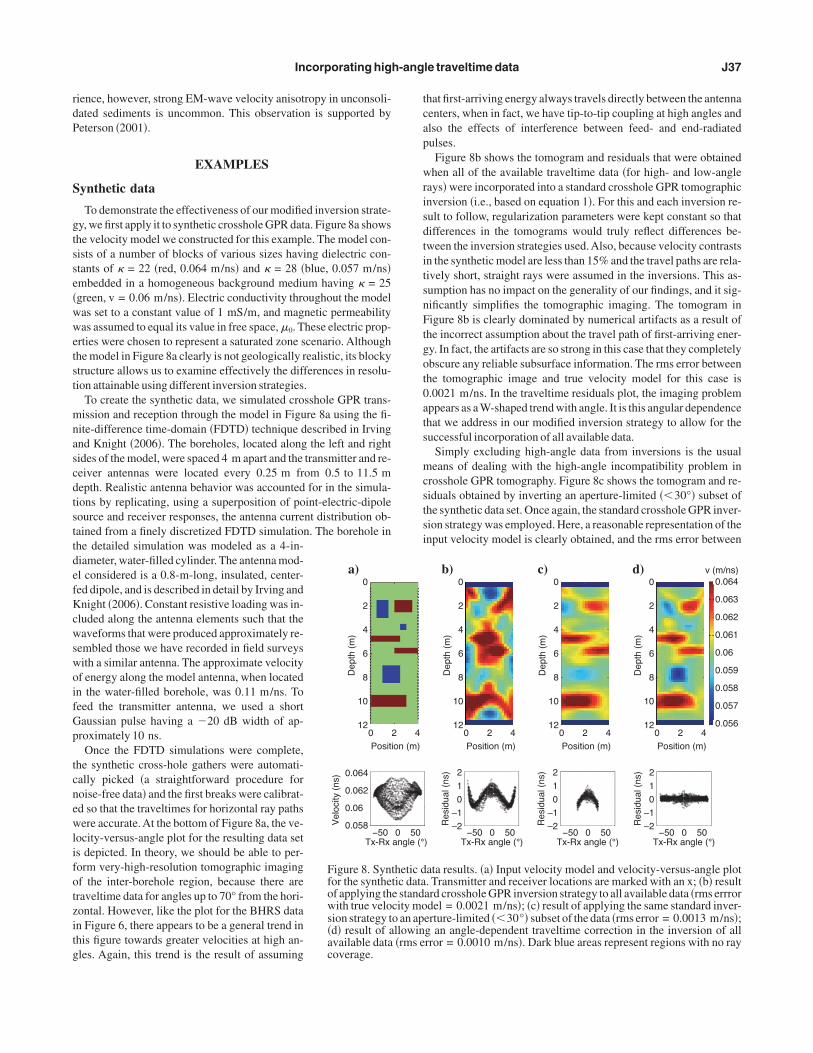
To demonstrate the effectiveness of our modified inversion strate-y, we first apply it to synthetic crosshole GPR data. Figure 8a showshe velocity model we constructed for this example. The model con-ists of a number of blocks of various sizes having dielectric con-tants of � = 22 �red, 0.064 m/ns� and � = 28 �blue, 0.057 m/ns�mbedded in a homogeneous background medium having � = 25green, v = 0.06 m/ns�. Electric conductivity throughout the modelas set to a constant value of 1 mS/m, and magnetic permeabilityas assumed to equal its value in free space, �0. These electric prop-
rties were chosen to represent a saturated zone scenario. Althoughhe model in Figure 8a clearly is not geologically realistic, its blockytructure allows us to examine effectively the differences in resolu-ion attainable using different inversion strategies.
To create the synthetic data, we simulated crosshole GPR trans-ission and reception through the model in Figure 8a using the fi-
ite-difference time-domain �FDTD� technique described in Irvingnd Knight �2006�. The boreholes, located along the left and rightides of the model, were spaced 4 m apart and the transmitter and re-eiver antennas were located every 0.25 m from 0.5 to 11.5 mepth. Realistic antenna behavior was accounted for in the simula-ions by replicating, using a superposition of point-electric-dipoleource and receiver responses, the antenna current distribution ob-ained from a finely discretized FDTD simulation. The borehole inhe detailed simulation was modeled as a 4-in-iameter, water-filled cylinder. The antenna mod-l considered is a 0.8-m-long, insulated, center-ed dipole, and is described in detail by Irving andnight �2006�. Constant resistive loading was in-
luded along the antenna elements such that theaveforms that were produced approximately re-
embled those we have recorded in field surveysith a similar antenna. The approximate velocityf energy along the model antenna, when locatedn the water-filled borehole, was 0.11 m/ns. Toeed the transmitter antenna, we used a shortaussian pulse having a �20 dB width of ap-roximately 10 ns.
Once the FDTD simulations were complete,he synthetic cross-hole gathers were automati-ally picked �a straightforward procedure foroise-free data� and the first breaks were calibrat-d so that the traveltimes for horizontal ray pathsere accurate. At the bottom of Figure 8a, the ve-
ocity-versus-angle plot for the resulting data sets depicted. In theory, we should be able to per-orm very-high-resolution tomographic imagingf the inter-borehole region, because there areraveltime data for angles up to 70° from the hori-ontal. However, like the plot for the BHRS datan Figure 6, there appears to be a general trend inhis figure towards greater velocities at high an-les. Again, this trend is the result of assuming
Vel
ocity
(ns
)
−50Tx-Rx
0.064
0.062
0.06
0.058
Posit0
Dep
th (
m)
0
2
4
6
8
10
12
a)
Figure 8. Synfor the syntheof applying thwith true velosion strategy t�d� result of aavailable datacoverage.
hat first-arriving energy always travels directly between the antennaenters, when in fact, we have tip-to-tip coupling at high angles andlso the effects of interference between feed- and end-radiatedulses.
Figure 8b shows the tomogram and residuals that were obtainedhen all of the available traveltime data �for high- and low-angle
ays� were incorporated into a standard crosshole GPR tomographicnversion �i.e., based on equation 1�. For this and each inversion re-ult to follow, regularization parameters were kept constant so thatifferences in the tomograms would truly reflect differences be-ween the inversion strategies used. Also, because velocity contrastsn the synthetic model are less than 15% and the travel paths are rela-ively short, straight rays were assumed in the inversions. This as-umption has no impact on the generality of our findings, and it sig-ificantly simplifies the tomographic imaging. The tomogram inigure 8b is clearly dominated by numerical artifacts as a result of
he incorrect assumption about the travel path of first-arriving ener-y. In fact, the artifacts are so strong in this case that they completelybscure any reliable subsurface information. The rms error betweenhe tomographic image and true velocity model for this case is.0021 m/ns. In the traveltime residuals plot, the imaging problemppears as a W-shaped trend with angle. It is this angular dependencehat we address in our modified inversion strategy to allow for theuccessful incorporation of all available data.
Simply excluding high-angle data from inversions is the usualeans of dealing with the high-angle incompatibility problem in
rosshole GPR tomography. Figure 8c shows the tomogram and re-iduals obtained by inverting an aperture-limited ��30°� subset ofhe synthetic data set. Once again, the standard crosshole GPR inver-ion strategy was employed. Here, a reasonable representation of thenput velocity model is clearly obtained, and the rms error between
Position (m)0 2 4
v (m/ns)
−50 0 50Tx-Rx angle (°)
−50 0 50Tx-Rx angle (°)
Res
idua
l (ns
) 2
1
0
–1
–2
Dep
th (
m)
0
2
4
6
8
10
12
Res
idua
l (ns
) 2
1
0
–1
–2−50 0 50
Tx-Rx angle (°))
Res
idua
l (ns
) 2
1
0
–1
–2
0.064
0.063
0.062
0.061
0.06
0.059
0.058
0.057
0.056
d)
Position (m)0 2 4
Dep
th (
m)
0
2
4
6
8
10
12
c)
Position (m)0 2 4
Dep
th (
m)
0
2
4
6
8
10
12
b)
ata results. �a� Input velocity model and velocity-versus-angle plot. Transmitter and receiver locations are marked with an x; �b� resultard crosshole GPR inversion strategy to all available data �rms errrordel = 0.0021 m/ns�; �c� result of applying the same standard inver-
erture-limited ��30°� subset of the data �rms error = 0.0013 m/ns�;g an angle-dependent traveltime correction in the inversion of allrror = 0.0010 m/ns�. Dark blue areas represent regions with no ray
0 50angle (°
ion (m)2 4
thetic dtic datae standcity moo an apllowin�rms e
t
il2Fbihtb
ol
pmifidct8
iiittptFwfdfts
Ft
Foototg
J38 Irving et al.
he recovered and true models decreases significantly to 0.0013m/ns. However, because we have not incorporated high-angle raysnto the inversion, horizontal resolution is compromised significant-y. Most noticeably, the high- and low-velocity anomalies around
m depth in Figure 8a are not separated from the edges of the grid inigure 8c; the small, low-velocity anomaly around 4 m depth cannote identified; and the large, low-velocity anomaly around 8 m depths smeared significantly in the horizontal direction. Although moreorizontal structure could be added to this tomogram by increasinghe cutoff angle for aperture limitation, we found that 30° yielded theest trade-off between an image containing horizontal structure and
−50 0 50 Tx-Rx angle (°)
Tra
velti
me
corr
ectio
n (n
s)
0
–1
–2
–3
–4
igure 9. Angle-dependent traveltime correction parameters ob-ained in the inversion of the synthetic data in Figure 8d.
−50 0 50Tx-Rx angle (°)
Res
idua
l (ns
)
Dep
th (
m)
Res
idua
l (ns
) 2
1
0
–1
–2−50 0 50
Tx-Rx angle (°)−50 0 50
Tx-Rx angle (°)
Res
idua
l (ns
) 2
1
0
–1
–2Res
idua
l (ns
) 2
1
0
–1
–2
d)
Position (m)0 2 4
Dep
th (
m)
c)
Position (m)0 2 4
Dep
th (
m)
b)
Position (m)0 2 4
Dep
th (
m)
4
6
8
10
12
14
16
18
4
6
8
10
12
14
16
18
4
6
8
10
12
14
16
18
a)
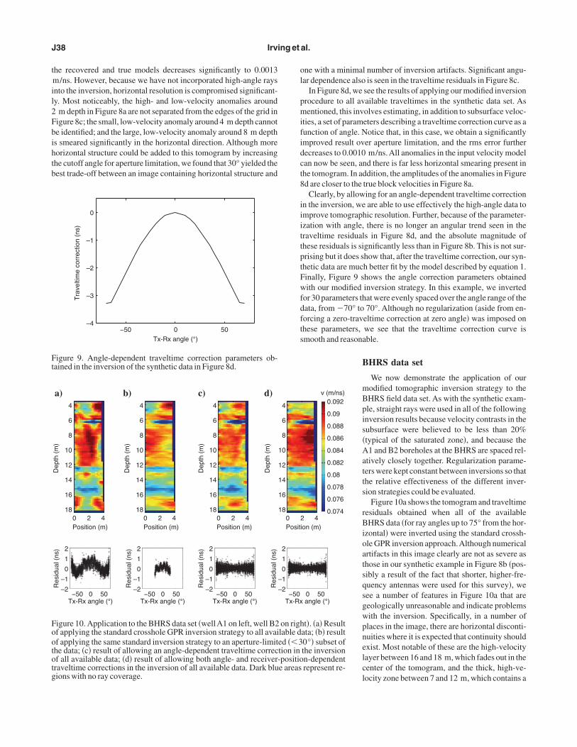
igure 10. Application to the BHRS data set �wellA1 on left, well B2f applying the standard crosshole GPR inversion strategy to all avaif applying the same standard inversion strategy to an aperture-limithe data; �c� result of allowing an angle-dependent traveltime correcf all available data; �d� result of allowing both angle- and receiverraveltime corrections in the inversion of all available data. Dark bluions with no ray coverage.
ne with a minimal number of inversion artifacts. Significant angu-ar dependence also is seen in the traveltime residuals in Figure 8c.
In Figure 8d, we see the results of applying our modified inversionrocedure to all available traveltimes in the synthetic data set. Asentioned, this involves estimating, in addition to subsurface veloc-
ties, a set of parameters describing a traveltime correction curve as aunction of angle. Notice that, in this case, we obtain a significantlymproved result over aperture limitation, and the rms error furtherecreases to 0.0010 m/ns. All anomalies in the input velocity modelan now be seen, and there is far less horizontal smearing present inhe tomogram. In addition, the amplitudes of the anomalies in Figured are closer to the true block velocities in Figure 8a.
Clearly, by allowing for an angle-dependent traveltime correctionn the inversion, we are able to use effectively the high-angle data tomprove tomographic resolution. Further, because of the parameter-zation with angle, there is no longer an angular trend seen in theraveltime residuals in Figure 8d, and the absolute magnitude ofhese residuals is significantly less than in Figure 8b. This is not sur-rising but it does show that, after the traveltime correction, our syn-hetic data are much better fit by the model described by equation 1.inally, Figure 9 shows the angle correction parameters obtainedith our modified inversion strategy. In this example, we inverted
or 30 parameters that were evenly spaced over the angle range of theata, from �70° to 70°. Although no regularization �aside from en-orcing a zero-traveltime correction at zero angle� was imposed onhese parameters, we see that the traveltime correction curve ismooth and reasonable.
BHRS data set
We now demonstrate the application of ourmodified tomographic inversion strategy to theBHRS field data set. As with the synthetic exam-ple, straight rays were used in all of the followinginversion results because velocity contrasts in thesubsurface were believed to be less than 20%�typical of the saturated zone�, and because theA1 and B2 boreholes at the BHRS are spaced rel-atively closely together. Regularization parame-ters were kept constant between inversions so thatthe relative effectiveness of the different inver-sion strategies could be evaluated.
Figure 10a shows the tomogram and traveltimeresiduals obtained when all of the availableBHRS data �for ray angles up to 75° from the hor-izontal� were inverted using the standard crossh-ole GPR inversion approach.Although numericalartifacts in this image clearly are not as severe asthose in our synthetic example in Figure 8b �pos-sibly a result of the fact that shorter, higher-fre-quency antennas were used for this survey�, wesee a number of features in Figure 10a that aregeologically unreasonable and indicate problemswith the inversion. Specifically, in a number ofplaces in the image, there are horizontal disconti-nuities where it is expected that continuity shouldexist. Most notable of these are the high-velocitylayer between 16 and 18 m, which fades out in thecenter of the tomogram, and the thick, high-ve-locity zone between 7 and 12 m, which contains a
ion (m)2 4
v (m/ns)
0 50 angle (°)
0.092
0.09
0.088
0.086
0.084
0.082
0.08
0.078
0.076
0.074
t�. �a� Resultata; �b� result0°� subset ofthe inversionn-dependentrepresent re-
Posit0
−50Tx-Rx
2
1
0
–1
–2
4
6
8
10
12
14
16
18
on righlable ded ��3tion in-positioe areas
ceai
tumcricrc
ofipsaiotrtfmtm
ftczcncwlc
tdtcttw0satr
da
wtRiissfcct
dtWdtlullsaatduaishbp
Fc1
Incorporating high-angle traveltime data J39
entral zone of significantly higher velocity. As with the syntheticxample, such problems are manifest in the traveltime residuals plots a distinct, W-shaped trend with angle. Such a trend should not ex-st for a proper tomographic inversion.
In Figure 10b, we see the result of applying aperture-limitation tohe BHRS data set before inverting. Again, a cutoff angle of 30° wassed to obtain the best trade-off between horizontal resolution and ainimal number of obvious inversion artifacts in the image. In this
ase, we see that the tomogram has become much more geologicallyeasonable. Layers are now more horizontally continuous and themage lacks the obvious problems seen in Figure 10a. However, be-ause we discarded the high-angle-ray data to produce the inversionesult in Figure 10b, we are left wondering whether such horizontalontinuity is real, or simply a product of the aperture limitation.
Figure 10c shows the tomogram and residuals obtained when allf the available BHRS traveltimes were incorporated into our modi-ed inversion procedure. Notice that, through the use of an angle-de-endent traveltime correction, we are now able to obtain a very rea-onable subsurface image that is quite similar in appearance to theperture-limited result in Figure 10b. For this example, it appears asf the addition of the high-angle data does not provide a large amountf additional structure to the tomogram �i.e., the geology betweenhe boreholes is such that it can be largely captured by the low-angle-ay data�. However, because we have used all available traveltimeso create the image in Figure 10c, we have greater confidence that theeatures seen here are representative of the true subsurface velocityodel. As with the synthetic example, the traveltime residuals ob-
ained using our modified inversion procedure are now approxi-ately flat with angle.Although we consider Figure 10c to be a much improved subsur-
ace image over Figure 10a, there is still something in this tomogramhat causes us concern given other geophysical and geologic dataollected at the BHRS. This is the fact that the thick, high-velocityone between 7 and 12 m depth, which is known to be a laterallyontinuous, poorly sorted sediment layer with relatively little inter-al variation in porosity �Barrash and Reboulet 2004�, shows signifi-ant lateral variability in Figure 10c. As a result of this observation,e investigated the effects of further parametrizing the inverse prob-
em to account for possible static traveltime shifts at the receiver lo-ations.
When collecting each gather in the BHRS data set, the receiver an-enna was held fixed while the transmitter antenna was loweredown its borehole. Because of this, the potential exists for manyraveltimes to be affected by a single error in the location of the re-eiver antenna in its well, or by differences in the coupling of this an-enna with its surroundings. For example, a horizontal movement ofhe receiver antenna in its well by only 2.5 cm �when the well is filledith water� will result in a shift in measured traveltime of at least.75 ns for all of the traces in that receiver gather. This shift is quiteignificant when the borehole spacing of only 3.5 m is considered. Inddition, slight drifts in the transmitter fire time over the duration ofhe crosshole survey can result in static time shifts between differenteceiver gathers.
To estimate traveltime corrections at each receiver location in ad-ition to slownesses and angle-correction parameters, we furtherugmented equation 2 as follows:
�t = �L A R�� �s
�pa
�pr� �3�
here the vector �pr contains receiver position traveltime correc-ions �i.e., a static correction for each receiver position�, and matrix
selects, for each ray, which correction to use. Inverting for staticsn this manner was shown by Vasco et al. �1997� to be a valuable tooln crosshole GPR tomography. Because there is no reason why suchtatic traveltime shifts should be smooth in depth, we added nomoothness regularization to the inversion. We did, however, en-orce smallness in the static correction parameters because a largeonstant traveltime shift for all receiver locations again could beompensated by appropriate angle-dependent traveltime correc-ions.
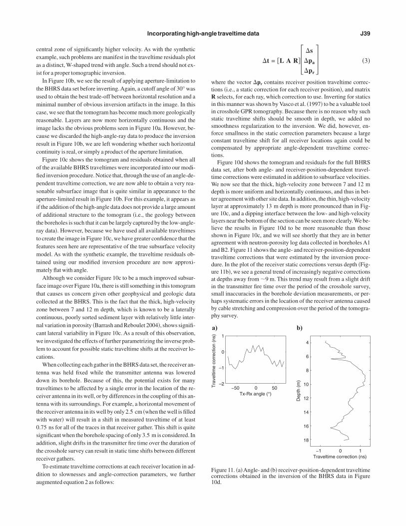
Figure 10d shows the tomogram and residuals for the full BHRSata set, after both angle- and receiver-position-dependent travel-ime corrections were estimated in addition to subsurface velocities.
e now see that the thick, high-velocity zone between 7 and 12 mepth is more uniform and horizontally continuous, and thus in bet-er agreement with other site data. In addition, the thin, high-velocityayer at approximately 13 m depth is more pronounced than in Fig-re 10c, and a dipping interface between the low- and high-velocityayers near the bottom of the section can be seen more clearly. We be-ieve the results in Figure 10d to be more reasonable than thosehown in Figure 10c, and we will see shortly that they are in bettergreement with neutron-porosity log data collected in boreholes A1nd B2. Figure 11 shows the angle- and receiver-position-dependentraveltime corrections that were estimated by the inversion proce-ure. In the plot of the receiver static corrections versus depth �Fig-re 11b�, we see a general trend of increasingly negative correctionst depths away from �9 m. This trend may result from a slight driftn the transmitter fire time over the period of the crosshole survey,mall inaccuracies in the borehole deviation measurements, or per-aps systematic errors in the location of the receiver antenna causedy cable stretching and compression over the period of the tomogra-hy survey.
−50 0 50 Tx-Rx angle (°)
Tra
velti
me
corr
ectio
n (n
s)
−1 0 1 Traveltime correction (ns)
Dep
th (
m)
1
0
–1
–2
4
6
8
10
12
14
16
18
a) b)
igure 11. �a�Angle- and �b� receiver-position-dependent traveltimeorrections obtained in the inversion of the BHRS data in Figure0d.

solrte
wpg
t=wh
FblwBacdt
trtbtcfmvemsnpi
ircnpoctjtlpmbdii
flhtchzrwo
a
F�tiA
J40 Irving et al.
As further verification of the validity of our tomographic inver-ion results, Figure 12 compares porosities obtained from the edgesf the tomograms in Figure 10c and d with neutron-porosity logs col-ected in wells A1 and B2 at the BHRS. To convert the tomographicadar velocities to porosity values for the figure, we first convertedhem to bulk dielectric-constant values using the following low-lossquation:
�b =c2
v2 , �4�
here c is the velocity of light in free space. We then used the com-lex refractive index �CRIM� model �e.g., Huisman et al., 2003�,iven by
�b = ��1 − ���s� + ��w
��1/� �5�
o relate the dielectric constant to porosity, �. Here, �s = 4 and �w
80 were used for the dielectric constants of the mineral grains andater, respectively, and we set � = 0.5. Solving equation 5 for �, weave:
0.1 0.2 0.3 0.4
Porosity
0.1 0.2 0.3 0.4
Porosity
Dep
th (
m)
Dep
th (
m)
4
6
8
10
12
14
16
18
4
6
8
10
12
14
16
18
) b)
igure 12. Comparison of neutron porosity log measurementsblack�, porosities calculated from velocites along the edges of theomogram in Figure 10c �red�, and porosities calculated from veloc-tes along the edges of the tomogram in Figure 10d �blue�. �a� Well1 �transmitter�; �b� Well B2 �receiver�.
� =�b
� − �s�
�w� − �s
� . �6�
igure 12 shows that, except for a marked difference in amplitudeecause of the inherent smoothing in the ray-based tomographic ve-ocity estimates, the tomographically derived porosities are quiteell correlated with the porosity logs from each borehole. For well2, we see that the tomographic results obtained using both angle-nd receiver-position-dependent traveltime corrections are a signifi-antly better match to the porosity data than the results with angle-ependent corrections alone. This further justifies our use of bothypes of traveltime corrections in creating Figure 10d.
CONCLUSIONS
Using an example data set from the BHRS, we have developedwo strategies for improving the resolution of crosshole GPR tomog-aphy at close borehole spacings. Together, these strategies allow uso take full advantage of the excellent angular coverage that suchorehole spacings can provide. For picking first breaks on very noisyraces at high transmitter/receiver angles, we have shown that arosscorrelation approach using angle-dependent reference wave-orms can be very effective.An important application of this pickingethod, not considered here, may be time-lapse crosshole GPR sur-
eying, where the S/N is commonly very low because stacking ofach trace is minimized for the sake of increased survey speed. Asentioned previously, our picking method performs best when
trong scattering in the data �interfering with the direct arrivals� isot present. Future work includes investigating whether such an ap-roach could be modified for effective use on other data sets contain-ng strongly scattered events.
To incorporate high-angle data into crosshole GPR tomographicnversions, we have shown that inverting for a small number of pa-ameters that describe an angle-dependent traveltime correctionurve, in addition to subsurface velocities, can be very effective. Weote again that this modified inversion procedure provided im-roved results with both synthetic and field data, despite the fact thatnly traveltimes were altered, and changes in survey geometry be-ause of tip-to-tip antenna coupling were thus ignored. If necessary,he tomographic sensitivity matrix in equations 1–3 could also be ad-usted to better account for end-to-end coupling above a certainhreshold angle. This may be required with lower-frequency �i.e.,onger antennas� data. An additional benefit of our inversion ap-roach is that it allows us to correct for the effects of errors in trans-itter fire time and borehole-location measurements. Although we
elieve that these measurements were very accurate for the BHRSata set, errors in these parameters also can result in apparent trendsn velocity with angle at close borehole spacings, and thus incompat-bility problems between high- and low-angle ray data.
Finally, we must stress that angular coverage is one of a number ofactors that affect resolution in crosshole GPR tomography. By al-owing for improved angular coverage with the methods presentedere, we have seen that significant increases in tomographic resolu-ion are possible. However, resolution with ray-based tomographyan only be improved to a certain point, as ray-based techniquesave an upper resolution limit of approximately the first Fresnelone associated with the GPR pulse bandwidth. In order to improveesolution past this limit, finite-frequency �Fresnel-zone� or full-aveform inversion methods must be employed. Regardless, the usef high-angle data and angle-dependent traveltime corrections �as
dd
t0DwOlnntf
A
B
B
B
B
C
C
E
H
H
I
—
—
L
L
M
M
M
P
P
P
P
R
S
S
S
T
T
T
V
V
W
Incorporating high-angle traveltime data J41
escribed in this study� are critical to maximize the resolution of ra-ar tomograms for hydrologic and environmental applications.
ACKNOWLEDGMENTS
This research was supported in part by funding to R. Knight fromhe National Science Foundation, Grant number EAR-0229896-02. J. Irving was also supported during part of this work through aepartmental Chair’s Fellowship at Stanford University. The cross-ell radar survey at the BHRS was funded by U. S. Army Researchffice Grant DAAG5-98-1-0277 to M. Knoll. The authors would
ike to thank Peter Annan for many helpful discussions about anten-as at the start of this research, and Warren Barrash for providing theeutron-porosity logs used in this study. The authors would also likeo thank reviewers Sherif Hanafy, John Lane, and George Tsofliasor feedback that improved the manuscript.
REFERENCES
lumbaugh, D., and P. Y. Chang, 2002, Estimating moisture contents in thevadose zone using cross-borehole ground-penetrating radar:Astudy of ac-curacy and repeatability: Water Resources Research, 38, 1309; http://dx.doi.org/10.1029/2001WR000754.
arrash, W., and T. Clemo, 2002, Hierarchical geostatistics and multi-faciessystems: Boise Hydrogeophysical Research Site, Boise, Idaho: Water Re-sources Research, 38, 1196; http://dx.doi.org/10.1029/2002WR001436.
arrash, W., T. Clemo, and M. D. Knoll, 1999, Boise Hydrogeophysical Re-search Site: Objectives, design, and initial geostatistical results: Proceed-ings, Symposium on the Application of Geophysics to Engineering andEnvironmental Problems, 389–398.
arrash, W., and M. D. Knoll, 1998, Design of research wellfield for calibrat-ing geophysical methods against hydrologic parameters: Proceedings,Conference on Hazardous Waste Research, Great Plains/Rocky Moun-tains HSRC, 296–318; http://cgiss.boisestate.edu/%7Ebille/BHRS/Papers/Barrash98/Design98. html, accessed May 21, 2007.
arrash, W., and E. C. Reboulet, 2004, Significance of porosity for stratigra-phy and textural composition in subsurface coarse fluvial deposits, BoiseHydrogeophysical Research Site: Geological Society ofAmerica Bulletin,116, 1059–1073; http://dx.doi.org/10.1130/B25370.1.
lement, W. P., and W. Barrash, 2006, Crosshole radar tomography in a fluvi-al aquifer near Boise, Idaho: Journal of Engineering and EnvironmentalGeophysics, 11, 171–184.
lement, W. P., W. Barrash, and M. D. Knoll, 2006, Reflectivity modeling ofground-penetrating radar: Geophysics, 71, no. 3, K59–K66.
llefsen, K. J., and D. L. Wright, 2005, Radiation pattern of a borehole radarantenna: Geophysics, 70, no. 1, K1–K11.
olliger, K., and T. Bergmann, 2002, Numerical modeling of borehole geo-radar data: Geophysics, 67, 1249–1257.
uisman, J. A., S. S. Hubbard, J. D. Redman, and A. P. Annan, 2003, Measur-ing soil water content with ground-penetrating radar: A review: VadoseZone Journal 2, 476–491.
rving, J. D., and R. J. Knight, 2005a, Effect of antennas on velocity estimates
obtained from crosshole GPR data: Geophysics, 70, no. 5, K39–K42.—–, 2005b, Accounting for the effect of antenna length to improve crossh-ole GPR velocity estimates: 75th Annual International Meeting, SEG, Ex-pandedAbstracts, 1188–1192.—–, 2006, Numerical simulation of antenna transmission and reception forcrosshole ground-penetrating radar: Geophysics, 71, no. 2, K37–K45.
inde, N., A. Binley, A. Tryggvason, L. B. Pedersen, and A. Revil, 2006, Im-proved hydrogeophysical characterization using joint inversion of cross-hole electrical resistance and ground-penetrating radar traveltime data:Water Resources Research, 42, W12404; http://dx.doi.org/10.1029/2006WR005131.
iu, S., and M. Sato, 2005, Transient radiation from an unloaded, finite di-pole antenna in a borehole: Experimental and numerical results: Geophys-ics, 70, no. 6, K43–K51.enke, W., 1984, The resolving power of cross-borehole tomography: Geo-physical Research Letters, 11, 105–108.olyneux, J. B., and D. R. Schmitt, 1999, First-break timing: Arrival onsettimes by direct correlation: Geophysics, 64, 1492–1501.oret, G. J. M., M. D. Knoll, W. Barrash, and W. P. Clement, 2006, Investi-gating the stratigraphy of an alluvial aquifer using crosswell seismic trav-eltime tomography: Geophysics, 71, no. 3, B63–B73.
eraldi, R., and A. Clement, 1972, Digital processing of refraction data:Study of first arrivals: Geophysical Prospecting, 20, 529–548.
eterson, J. E., 2001, Pre-inversion corrections and analysis of radar tomog-raphic data: Journal of Environmental and Engineering Geophysics, 6,1–18.
ratt, R. G., and N. R. Goulty, 1991, Combining wave-equation imaging withtravel-time tomography to form high-resolution images from crossholedata: Geophysics, 56, 208–224.
ratt, R. G., and M. H. Worthington, 1988, The application of diffraction to-mography to cross-hole seismic data: Geophysics, 53, 1284–1294.
ector, J. W., and J. K. Washbourne, 1994, Characterization of resolution anduniqueness in crosswell direct-arrival traveltime tomography using theFourier projection-slice theorem: Geophysics, 59, 1642–1649.
ato, M., and R. Thierbach, 1991, Analysis of a borehole radar in cross-holemode: IEEE Transactions on Geoscience and Remote Sensing, 29,899–904.
cales, J. A., 1987, Tomographic inversion via the conjugate gradient meth-od: Geophysics, 52, 179–185.
quires, L. J., S. N. Blakeslee, and P. L. Stoff, 1992, The effects of statics ontomographic velocity reconstructions: Geophysics, 57, 353–362.
ronicke, J., P. Dietrich, and E. Appel, 2002a, Quality improvement of cross-hole georadar tomography: Pre- and post-inversion data analysis strate-gies: European Journal of Environmental and Engineering Geophysics, 7,59–73.
ronicke, J., P. Dietrich, U. Wahlig, and E. Appel, 2002b, Integrating surfacegeoradar and crosshole radar tomography: A validation experiment inbraided stream deposits: Geophysics, 67, 1516–1523.
ronicke, J., K. Holliger, W. Barrash, and M. D. Knoll, 2004, Multivariateanalysis of cross-hole georadar velocity and attenuation tomograms foraquifer zonation: Water Resources Research, 40, W01519; http://dx.doi.org/10.1029/2003WR002031.
anDecar, J., and R. Crosson, 1990, Determination of teleseismic relativephase arrival times using multi-channel cross-correlation and leastsquares: Bulletin of the Seimological Society ofAmerica, 80, 150–159.
asco, D. W., J. E. Peterson, and K. H. Lee, 1997, Ground-penetrating radarvelocity tomography in heterogeneous anisotropic media: Geophysics, 62,1758–1773.oodward, R. L., and G. Masters, 1991, Global upper mantle structure fromlong-period differential arrival times: Journal of Geophysical Research,
96, 6351–6377.