“improvement of energy reconstruction by using … · kazuma ishio, max-planck-institut für...
TRANSCRIPT
KazumaIshio,Max-Planck-InstitutfürPhysik27. März. 2017, DPG-Frühjahrstagung Münster T 23.6
“ I m p ro v e m e n t o f e n e rg y re c o n s t r u c t i o n b y u s i n g m a c h i n e l e a r n i n g a l g o r i t h m s i n M A G I C ”
Kazuma Ish io , Dav id Paneque Max-P lanck - Inst i tut für Phys ik Ga l ina Maneva, Petar Temnikov Inst i tute for Nuc lear Research and Nuc lear Energy, Sof ia , Bu lgar ia Abelardo Mora le jo Inst i tut de F is i ca d 'A l tes Energ ies ( IFAE) , The Barce lona Inst i tute of Sc ience and Technology, Be l laterra (Barce lona) , Spa in Ju l ian S i tarek D iv i s ion of Astrophys ics , Un ivers i ty of Lodz, Lodz, Po land

Kazuma Ishio, Max-Planck-Institut für Physik 27, März. 2017,DPG Münster
U n i v e r s e i s b r i g h t i n G a m m a r a y s
2
https://svs.gsfc.nasa.gov/Sky map in energy range 50GeV - 2TeV by Fermi satellite
@ “vicinity”
Pulsars and PWN
SuperNova Remnants
@ distant galaxies
GRBsAGNs

Kazuma Ishio, Max-Planck-Institut für Physik 27, März. 2017,DPG Münster
A n o t h e r p o s s i b l e s o u r c e — “ D a r k M a t t e r ”
3
http://wwwmpa.mpa-garching.mpg.de/galform

Kazuma Ishio, Max-Planck-Institut für Physik 27, März. 2017,DPG Münster
A n o t h e r p o s s i b l e s o u r c e — “ D a r k M a t t e r ”
4
log10(Energy)
Flux
or c
oun
ts
Background
5
In the last part of this section, let us briefly describehow we implemented IB from the various possible finalstates of neutralino annihilations in DarkSUSY. The totalgamma-ray spectrum is given by
dNγ,tot
dx=!
f
Bf
"dNγ,sec
f
dx+
dNγ,IBf
dx+
dNγ,line
f
dx
#
,
(10)where Bf denotes the branching ratio into the annihi-lation channel f . The last term in the above equationgives the contribution from the direct annihilation intophotons, γγ or Zγ, which result in a sharp line feature[27]. The first term encodes the contribution from sec-ondary photons, produced in the further decay and frag-mentation of the annihilation products, mainly throughthe decay of neutral pions. This “standard” part of thetotal gamma-ray yield from dark matter annihilationsshows a feature-less spectrum with a rather soft cutoffat Eγ = mχ. In DarkSUSY, these contributions are in-cluded by using the Monte Carlo code PYTHIA [28] tosimulate the decay of a hypothetical particle with mass2mχ and user-specified branching ratios Bf . In this way,also FSR associated to this decay is automatically in-cluded (the main contribution here comes from photonsdirectly radiated off the external legs, but also photonsradiated from other particles in the decay cascade aretaken into account). On the other hand, IB from thedecay of such a hypothetical particle cannot in generalbe expected to show the same characteristics as IB fromthe actual annihilation of two neutralinos. In particular,and as discussed in length at the beginning of this Sec-tion, we expect important VIB contributions in the lattercase – while in the first case there are simply no virtualparticles that could radiate photons. We therefore calcu-late analytically the IB associated to the decay (i.e. FSRfrom the final legs) and subtract it from dNγ,sec
f /dx as
obtained with PYTHIA; for dNγ,IBf /dx, we then take the
full IB contribution from the actual annihilation processas described before. Hence, this procedure leaves us withcorrected PYTHIA results without FSR on the externallegs and our analytical calculation of IB (including FSRand VIB) that we add to this. 1
Let us conclude this section by showing in Fig. 2 four
1 We would like to stress that this prescription is fully consistentsince both the original and the corrected IB versions are gauge-invariant separately. Strictly speaking, however, we have onlycorrected for photons originating directly from the external statesand not for those radiated from particles that appear later in thedecay cascade. On the other hand, one would of course expectthat modifying the energy distribution of the charged particlescorresponding to these external legs also affects the further de-cay cascade. Note, however, that the resulting change in thephoton spectrum is a second order effect; more important, forkinematical reasons it does not affect photons at energies closeto mχ – which, as we shall see, are the most relevant. Finally, weobserve that our subtraction procedure has only a minor effecton the photon spectrum obtained by PYTHIA and no practical
PSfrag
x = Eγ/mχ
x2dN
γ,t
ot/d
x
TotalSecondary gammasInternal Bremsstrahlung
0.4 0.6 0.8 1
1
0.001
0.01
0.1
0.2
BM1
.
0.01
x = Eγ/mχ
x2dN
γ,t
ot/d
x
TotalSecondary gammasInternal Bremsstrahlung
0.4 0.6 0.8 1
1
0.1
0.2
BM2
.
0.01
0.1
x = Eγ/mχ
x2dN
γ,t
ot/d
x
TotalSecondary gammasInternal Bremsstrahlung
0.4 0.6 0.8 1
0.001
1
10
0.2
BM3
.
0.01
0.1
x = Eγ/mχ
x2dN
γ,t
ot/d
x
TotalSecondary gammasInternal Bremsstrahlung
0.4 0.6 0.8 1
0.001
1
0.2
BM4
.
FIG. 2: From top to bottom, the gamma-ray spectra for thebenchmark models defined in Tab. I is shown. The contribu-tions from IB and secondary photons is indicated separately(in these figures, the line signal is not included).
Internal bremsstrahlung from produced charged particles
in the annihilations could yield a detectable ”bump”.
Additional feature in a spectrum to be searched
Bringmann,2008
S =
Ns!
Nb

Kazuma Ishio, Max-Planck-Institut für Physik 27, März. 2017,DPG Münster
F o r D M s e a r c h , e n e r g y r e s o l u t i o n “ m a t t e r s ”
5
log10(Energy)
Flux
or c
oun
ts
Background
5
In the last part of this section, let us briefly describehow we implemented IB from the various possible finalstates of neutralino annihilations in DarkSUSY. The totalgamma-ray spectrum is given by
dNγ,tot
dx=!
f
Bf
"dNγ,sec
f
dx+
dNγ,IBf
dx+
dNγ,line
f
dx
#
,
(10)where Bf denotes the branching ratio into the annihi-lation channel f . The last term in the above equationgives the contribution from the direct annihilation intophotons, γγ or Zγ, which result in a sharp line feature[27]. The first term encodes the contribution from sec-ondary photons, produced in the further decay and frag-mentation of the annihilation products, mainly throughthe decay of neutral pions. This “standard” part of thetotal gamma-ray yield from dark matter annihilationsshows a feature-less spectrum with a rather soft cutoffat Eγ = mχ. In DarkSUSY, these contributions are in-cluded by using the Monte Carlo code PYTHIA [28] tosimulate the decay of a hypothetical particle with mass2mχ and user-specified branching ratios Bf . In this way,also FSR associated to this decay is automatically in-cluded (the main contribution here comes from photonsdirectly radiated off the external legs, but also photonsradiated from other particles in the decay cascade aretaken into account). On the other hand, IB from thedecay of such a hypothetical particle cannot in generalbe expected to show the same characteristics as IB fromthe actual annihilation of two neutralinos. In particular,and as discussed in length at the beginning of this Sec-tion, we expect important VIB contributions in the lattercase – while in the first case there are simply no virtualparticles that could radiate photons. We therefore calcu-late analytically the IB associated to the decay (i.e. FSRfrom the final legs) and subtract it from dNγ,sec
f /dx as
obtained with PYTHIA; for dNγ,IBf /dx, we then take the
full IB contribution from the actual annihilation processas described before. Hence, this procedure leaves us withcorrected PYTHIA results without FSR on the externallegs and our analytical calculation of IB (including FSRand VIB) that we add to this. 1
Let us conclude this section by showing in Fig. 2 four
1 We would like to stress that this prescription is fully consistentsince both the original and the corrected IB versions are gauge-invariant separately. Strictly speaking, however, we have onlycorrected for photons originating directly from the external statesand not for those radiated from particles that appear later in thedecay cascade. On the other hand, one would of course expectthat modifying the energy distribution of the charged particlescorresponding to these external legs also affects the further de-cay cascade. Note, however, that the resulting change in thephoton spectrum is a second order effect; more important, forkinematical reasons it does not affect photons at energies closeto mχ – which, as we shall see, are the most relevant. Finally, weobserve that our subtraction procedure has only a minor effecton the photon spectrum obtained by PYTHIA and no practical
PSfrag
x = Eγ/mχ
x2dN
γ,t
ot/d
x
TotalSecondary gammasInternal Bremsstrahlung
0.4 0.6 0.8 1
1
0.001
0.01
0.1
0.2
BM1
.
0.01
x = Eγ/mχ
x2dN
γ,t
ot/d
x
TotalSecondary gammasInternal Bremsstrahlung
0.4 0.6 0.8 1
1
0.1
0.2
BM2
.
0.01
0.1
x = Eγ/mχ
x2dN
γ,t
ot/d
x
TotalSecondary gammasInternal Bremsstrahlung
0.4 0.6 0.8 1
0.001
1
10
0.2
BM3
.
0.01
0.1
x = Eγ/mχ
x2dN
γ,t
ot/d
x
TotalSecondary gammasInternal Bremsstrahlung
0.4 0.6 0.8 1
0.001
1
0.2
BM4
.
FIG. 2: From top to bottom, the gamma-ray spectra for thebenchmark models defined in Tab. I is shown. The contribu-tions from IB and secondary photons is indicated separately(in these figures, the line signal is not included).
S =
Ns!
Nb ×1/42×
If energy resolution becomes 4 times better,
significance would be double!
Bringmann,2008
Internal bremsstrahlung from produced charged particles
in the annihilations could yield a detectable ”bump”.

Kazuma Ishio, Max-Planck-Institut für Physik 27, März. 2017,DPG Münster
Te V g a m m a r a y w i t h M A G I C t e l e s c o p e
6
La Palma(29◦N, 18◦W), asl. 2200m Imaging Atmospheric Cherenkov Telescope (IACT) 2 telescopes with - Dish diameter : 17m - Camera FoV : 3.5deg - Trigger Threshold of gamma ray : ~50 GeV - Sensitivity : ~0.7% Crab flux 0.2TeV

Kazuma Ishio, Max-Planck-Institut für Physik 27, März. 2017,DPG Münster
H o w e n e r g y i s e s t i m a t e d ?
7
What is “Imaging Atmospheric Cherenkov Telescope (IACT)” ?
-The higher the gamma ray’s energy, the more the secondary particles, and hence the brighter the image of the shower (cherenkov light)
A high energy particle interacts with atmosphere, which initiates “air shower”, consists of so many secondary particles traveling faster than speed of light in the air.
Cherenkov radiation
- 104 times higher sensitivity than satellites !

Kazuma Ishio, Max-Planck-Institut für Physik 27, März. 2017,DPG Münster
T h e h i g h e r t h e g a m m a r a y ’s e n e r g y, t h e b r i g h t e r t h e s h o w e r i m a g e . B u t … l o c a t i o n m a t t e r s !
8
FoVFoV
Darker when more distant. —> correction with geometrical information is needed
Air shower

Kazuma Ishio, Max-Planck-Institut für Physik 27, März. 2017,DPG Münster
14/2007. June 2016
How to identify a �-ray
LengthWidth
Distance
Centre ofGravityTrue
Direction
ReconstructedDirection
Camera centre
Image of Telescope 2
Displacement
Image of Telescope 1
P a r a m e t r i s a t i o n
9
For each event, a vector value is stored with many components. - Brightness (light content) directly indicates initial energy. It needs to be corrected by the location parameters. - Shape useful for background rejection. - Orientation and location important for correction.
Energy can be estimated from light content corrected by location parameter etc.
=> 15 components are used in the Look Up Table method
Performance should improve by adopting machine learning
Kazuma Ishio, Max-Planck-Institut für Physik 27, März. 2017,DPG Münster
S p e c i f i c a t i o n s o f t h e A N N & R F
10
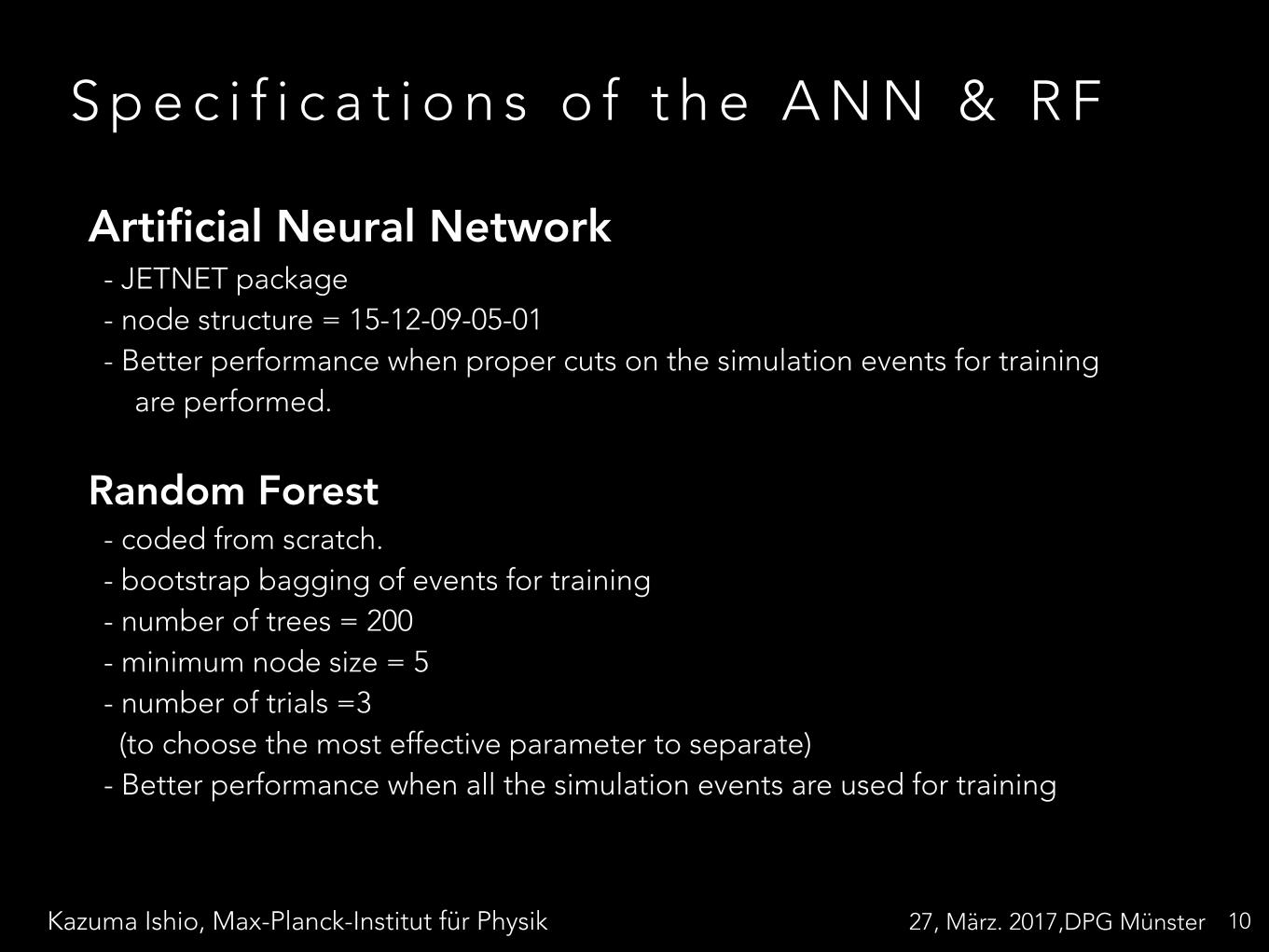
Artificial Neural Network - JETNET package - node structure = 15-12-09-05-01 - Better performance when proper cuts on the simulation events for training are performed.
Random Forest - coded from scratch. - bootstrap bagging of events for training - number of trees = 200 - minimum node size = 5 - number of trials =3 (to choose the most effective parameter to separate) - Better performance when all the simulation events are used for training

Kazuma Ishio, Max-Planck-Institut für Physik 27, März. 2017,DPG Münster
P e r f o r m a n c e e v a l u a t i o n
11
simulation data
Create estimator
estimator ( LUT/ ANN/ RF )
simulation data
Apply estimator
estimated energy
estimated energy should be the same as original energy
Kazuma Ishio, Max-Planck-Institut für Physik 27, März. 2017,DPG Münster
P e r f o r m a n c e e v a l u a t a i o n
12
true)/Etrue-E
est(E
1− 0.5− 0 0.5 1 1.5 2
# of
eve
nts
0
2
4
6
8
10
[GeV] bin 1.65+/- 0.05BiasDistribution of 10
273
[GeV] bin 1.65+/- 0.05BiasDistribution of 10
true)/Etrue-E
est(E
1− 0.5− 0 0.5 1 1.5 2
# of
eve
nts
0
2
4
6
8
10
12
14
16
18
20
[GeV] bin 1.75+/- 0.05BiasDistribution of 10
792
[GeV] bin 1.75+/- 0.05BiasDistribution of 10
true)/Etrue-E
est(E
1− 0.5− 0 0.5 1 1.5 2
# of
eve
nts
0
5
10
15
20
25
30
35
40
45
[GeV] bin 1.84+/- 0.05BiasDistribution of 10
1777
[GeV] bin 1.84+/- 0.05BiasDistribution of 10
true)/Etrue-E
est(E
1− 0.5− 0 0.5 1 1.5 2
# of
eve
nts
0
10
20
30
40
50
60
70
80
[GeV] bin 1.94+/- 0.05BiasDistribution of 10
3209
[GeV] bin 1.94+/- 0.05BiasDistribution of 10
true)/Etrue-E
est(E
1− 0.5− 0 0.5 1 1.5 2
# of
eve
nts
0
20
40
60
80
100
120
[GeV] bin 2.03+/- 0.05BiasDistribution of 10
4823
[GeV] bin 2.03+/- 0.05BiasDistribution of 10
true)/Etrue-E
est(E
1− 0.5− 0 0.5 1 1.5 2
# of
eve
nts
0
20
40
60
80
100
120
140
160
180
[GeV] bin 2.13+/- 0.05BiasDistribution of 10
6599
[GeV] bin 2.13+/- 0.05BiasDistribution of 10
true)/Etrue-E
est(E
1− 0.5− 0 0.5 1 1.5 2
# of
eve
nts
0
50
100
150
200
250
[GeV] bin 2.22+/- 0.05BiasDistribution of 10
8099
[GeV] bin 2.22+/- 0.05BiasDistribution of 10
true)/Etrue-E
est(E
1− 0.5− 0 0.5 1 1.5 2
# of
eve
nts
0
50
100
150
200
250
300
[GeV] bin 2.32+/- 0.05BiasDistribution of 10
9380
[GeV] bin 2.32+/- 0.05BiasDistribution of 10
true)/Etrue-E
est(E
1− 0.5− 0 0.5 1 1.5 2
# of
eve
nts
0
50
100
150
200
250
300
350
[GeV] bin 2.42+/- 0.05BiasDistribution of 10
10309
[GeV] bin 2.42+/- 0.05BiasDistribution of 10
true)/Etrue-E
est(E
1− 0.5− 0 0.5 1 1.5 2
# of
eve
nts
0
50
100
150
200
250
300
350
400
[GeV] bin 2.51+/- 0.05BiasDistribution of 10
10964
[GeV] bin 2.51+/- 0.05BiasDistribution of 10
true)/Etrue-E
est(E
1− 0.5− 0 0.5 1 1.5 2
# of
eve
nts
0
50
100
150
200
250
300
350
400
450
[GeV] bin 2.61+/- 0.05BiasDistribution of 10
11406
[GeV] bin 2.61+/- 0.05BiasDistribution of 10
true)/Etrue-E
est(E
1− 0.5− 0 0.5 1 1.5 2
# of
eve
nts
0
100
200
300
400
500
[GeV] bin 2.70+/- 0.05BiasDistribution of 10
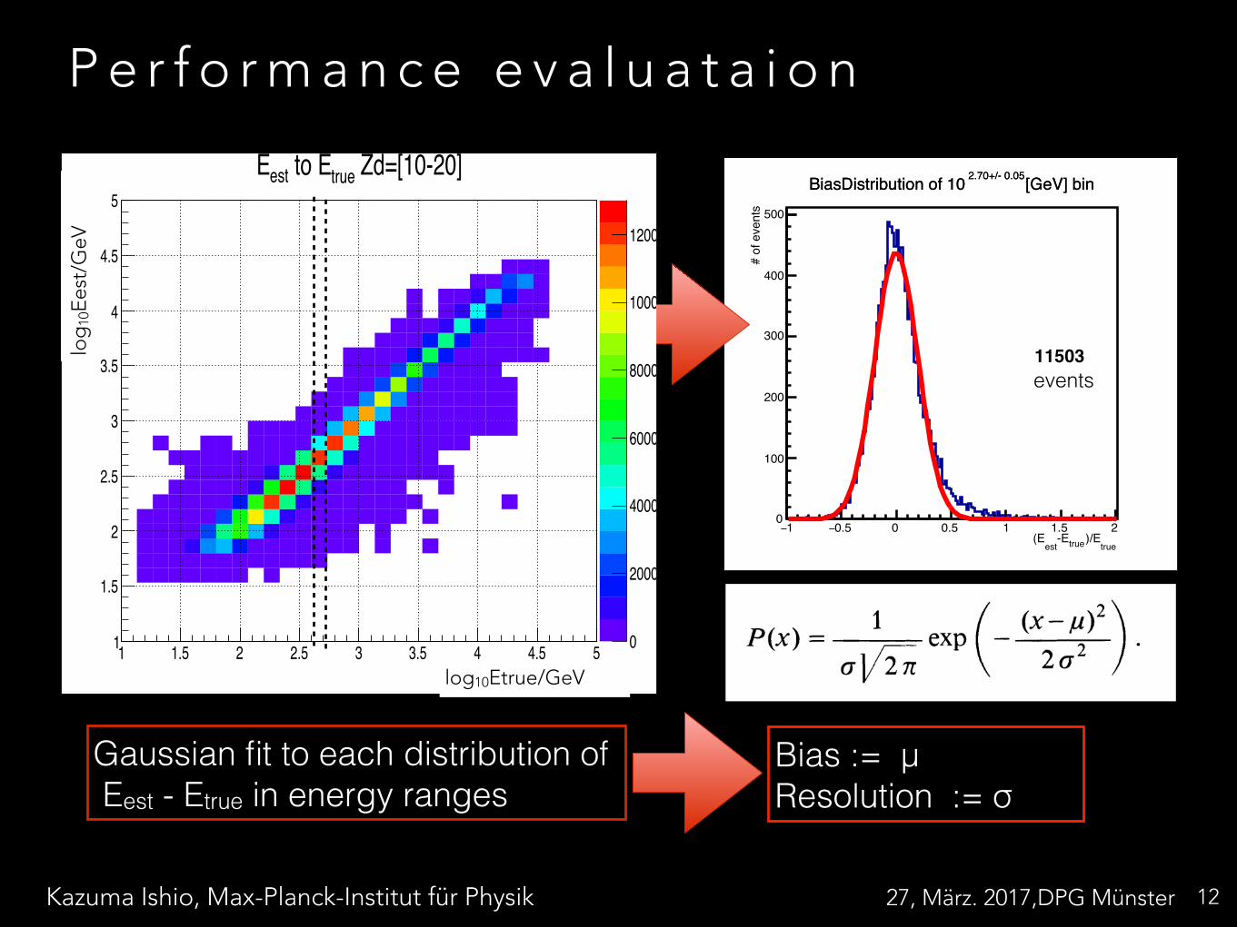
11503
[GeV] bin 2.70+/- 0.05BiasDistribution of 10
events
/GeV )est
( E10
log1 1.5 2 2.5 3 3.5 4 4.5 5
/Ge
V )
true
( E
10
log
1
1.5
2
2.5
3
3.5
4
4.5
5
0
2000
4000
6000
8000
10000
12000
Zd=[10-20]true to EestE 0 MARS - Magic Analysis and Reconstruction Software - Thu Mar 16 18:31:39 2017 Page No. 1
log10Etrue/GeV
log
10Ee
st/G
eV
4.2 Some Common Probability Distributions
Fig. 4.3. The Gaussian distribution for various G. The standard deviation determines the width of the distribution
87
---=-----------------
Fig. 4.4. Relation between the standard deviation G and the full width at half-maximum (FWHM)
instrumental errors are generally described by this probability distribution. Moreover, even in cases where its application is not strictly correct, the Gaussian often provides a good approximation to the true governing distribution.
The Gaussian is a continuous, symmetric distribution whose density is given by
P(x) = 1 exp (_ (x- . 20
(4.19)
The two parameters fl and 0 2 can be shown to correspond to the mean and variance of the distribution by applying (4.8) and (4.9).
The shape of the Gaussian is shown in Fig. 4.3. which illustrates this distribution for various o. The significance of 0 as a measure of the distribution width is clearly seen. As can be calculated from (4.19), the standard deviation corresponds to the half width of the peak at about 60070 of the full height. In some applications, however, the full width at half maximum (FWHM) is often used instead. This is somewhat larger than 0 and can easily be shown to be
FWHM = 20 V2ln 2 = 2.350. (4.20)
This is illustrated in Fig. 4.4. In such cases, care should be taken to be clear about which parameter is being used. Another width parameter which is also seen in the liter-ature is the full-width at one-tenth maximum (FWTM).
The integral distribution for the Gaussian density, unfortunately, cannot be cal-culated analytically so that one must resort to numerical integration. Tables of integral values are readily found as well. These are tabulated in terms of a reduced Gaussian distribution with fl = 0 and 0 2 = 1. All Gaussian distributions may be transformed to this reduced form by making the variable transformation
x-fl Z=--, (4.21)
o
where fl and 0 are the mean and standard deviation of the original distribution. It is a trivial matter then to verify that Z is distributed as a reduced Gaussian.
Gaussian fit to each distribution of Eest - Etrue in energy ranges
Bias := μ Resolution := σ

Kazuma Ishio, Max-Planck-Institut für Physik 27, März. 2017,DPG Münster
I m p r o v e m e n t b y m a c h i n e l e a r n i n g
13
Comparison of resolutions of Eest
log(True energy/GeV) 2 2.5 3 3.5 4
tru
e)/E
true
- E
est
(E
∆
0
0.1
0.2
0.3
0.4
0.5
0.6
LUTRFANN
Comparison of resolutions of Eest
Better resolution above ~200GeV
than the LUT (Current standard
in MAGIC)
Both machine learning techniques perform
very similarly

Kazuma Ishio, Max-Planck-Institut für Physik 27, März. 2017,DPG Münster
S a n i t y c h e c k ( i n R F s t r a t e g y )
14
/GeV )est
( E10
log1 1.5 2 2.5 3 3.5 4 4.5 5
Leng
th
0
50
100
150
200
250
300
0
200
400
600
800
1000
1200
1400
1600
Length_M1 MC Zd=[10-20]
/GeV )est
( E10
log1 1.5 2 2.5 3 3.5 4 4.5 5
Leng
th
0
50
100
150
200
250
300
0
500
1000
1500
2000
2500
3000
Length_M1 On-Off Zd=[10-20]
/GeV )est
( E10
log1 1.5 2 2.5 3 3.5 4 4.5 5
Leng
th
0
50
100
150
200
250
300
0.5−
0.4−
0.3−
0.2−
0.1−
0
0.1
0.2
0.3
0.4
0.5
MC - Rescaled(On-Off)
1 1.5 2 2.5 3 3.5 4 4.5 50
50
100
150
200
250
300
MCOn-Off
GausFit to distributions
3 MARS - Magic Analysis and Reconstruction Software - Thu Mar 23 01:22:44 2017 Page No. 4 An example of the comparison:MaxHeight (Zd =[10,20]deg)
real data (On - Off)MC
subtraction indicates similar distribution
All the parameter should distribute similarly under the same estimated energy and incoming direction.

Kazuma Ishio, Max-Planck-Institut für Physik 27, März. 2017,DPG Münster
S u m m a r y a n d C o n c l u s i o n s
15
Gamma-ray astronomy is a novel discipline that addresses many scientific topics. A good energy resolution can play important roles in many scientific studies (e.g. identification of bumps).
In IACT technique, the gamma-ray energy is derived from many image parameters. It is an excellent case for a room to be improved by machine learning techniques.
We have developed strategies and tools for the application of machine learning techniques (ANN and RF) for the reconstruction of the gamma-ray energy in MAGIC data.
When compared with the LUTs (standard method used in MAGIC), both ANN and RF show a performance improvement above 0.2 TeV, with a factor ~2 improvement at multi-TeV energies. In case of bump-like feature search, up to 40% higher significance can be expexted.

B A C K U P

Kazuma Ishio, Max-Planck-Institut für Physik 27, März. 2017,DPG Münster
~ 2 0 0 e m i t e v e n h i g h e r e n e r g y !
17
The sources which are detected by IACT : “Imaging Atmospheric Cherenkov Telescopes”
which are x104 more sensitive than satellites!
http://tevcat.uchicago.edu/Unidentified
Active Galactic Nuclei
Starburst Galaxy
Extragalactic sources
Pulsar Wind Nebula
Compact object (Pulsars,binaries etc.)
Super Nova Remnant
Star forming region Globular cluster
Galactic sources
Source types

Kazuma Ishio, Max-Planck-Institut für Physik 27, März. 2017,DPG Münster
A r t i f i c i a l N e u r a l N e t w o r k ( A N N )
18
for one of the perceptrons?
The architecture of neural networksIn the next section I'll introduce a neural network that can do apretty good job classifying handwritten digits. In preparation forthat, it helps to explain some terminology that lets us namedifferent parts of a network. Suppose we have the network:
As mentioned earlier, the leftmost layer in this network is called theinput layer, and the neurons within the layer are called inputneurons. The rightmost or output layer contains the outputneurons, or, as in this case, a single output neuron. The middlelayer is called a hidden layer, since the neurons in this layer areneither inputs nor outputs. The term "hidden" perhaps sounds alittle mysterious - the first time I heard the term I thought it musthave some deep philosophical or mathematical significance - but itreally means nothing more than "not an input or an output". Thenetwork above has just a single hidden layer, but some networkshave multiple hidden layers. For example, the following four-layernetwork has two hidden layers:
Somewhat confusingly, and for historical reasons, such multiplelayer networks are sometimes called multilayer perceptrons orMLPs, despite being made up of sigmoid neurons, not perceptrons.
σ : “Activation function”such as Sigmoid function
And we use for the activation of the neuron in the layer.The following diagram shows examples of these notations in use:
With these notations, the activation of the neuron in the layer is related to the activations in the layer by theequation (compare Equation (4) and surrounding discussion in thelast chapter)
where the sum is over all neurons in the layer. To rewritethis expression in a matrix form we define a weight matrix foreach layer, . The entries of the weight matrix are just the weightsconnecting to the layer of neurons, that is, the entry in the rowand column is . Similarly, for each layer we define a biasvector, . You can probably guess how this works - the componentsof the bias vector are just the values , one component for eachneuron in the layer. And finally, we define an activation vector whose components are the activations .
The last ingredient we need to rewrite (23) in a matrix form is theidea of vectorizing a function such as . We met vectorizationbriefly in the last chapter, but to recap, the idea is that we want toapply a function such as to every element in a vector . We use theobvious notation to denote this kind of elementwise applicationof a function. That is, the components of are just .As an example, if we have the function then the vectorizedform of has the effect
that is, the vectorized just squares every element of the vector.
With these notations in mind, Equation (23) can be rewritten in the
Weight wjk(Strength of connection)
The output of j th node in l th layeris the activation function σ
Input ak(output of k th node in l-1 th layer)
l-1
bias bj
The network can become almost any kind of nonlinear function

Kazuma Ishio, Max-Planck-Institut für Physik 27, März. 2017,DPG Münster
R a n d o m F o r e s t ( R F )
19https://www.quora.com/How-does-random-forest-work-for-regression-1
Ankit Sharma
A decision Tree classifies events by energy classes.
102 CHAPTER 5. THE RANDOM FOREST METHOD
Eest =qn≠1
i=0
Ei ·Niqn≠1
i=0
Ni(5.22)
In the application of RF each tree returns an estimated energy and the overall meanis calculated as the final estimated energy.
• Splitting rule based on the continuous quantityIt is possible to completely avoid the use of classes by introducing a splitting rule,which does not rely on class populations.The idea of the Gini-index (with its interpretation as binomial variance of theclasses) as split rule is a purification of the class populations, i.e. a separationof the classes, in the subsamples after the split process. Similarly, when using thevariance in energy as split criterion, the subsamples are purified with respect totheir energy distribution.
‡2(E) = 1N ≠ 1
Nÿ
i=1
(Ei ≠ E)2 = 1N ≠ 1 ·
CANÿ
i=1
E2
i
B
≠N · E2
D
(5.23)
In analogy to the Gini-index of the split, the ‘variance’ of the split is calculated byadding the ‘subsample energy variances’ taking into account the node populationsas weights:
‡2(E) = 1NL +NR
(NL‡2
L(E) +NR‡2
R(E)) (5.24)
5.5.1 Performance of the RF energy estimationIn the following the results of the RF energy estimation are presented using the CrabNebula-like gamma Monte Carlo sample, which was already described in section 5.4. Butnow the energy range of 10GeV < E < 30TeV is taken since there is no need for adoptingto a proton MC. The following quality cuts were imposed on this sample:
• Static dist cut: dist > 0.3¶
• Leakage cut: leakage < 0.1
These cuts remove events, which provide only a weak basis for an energy estima-tion, since the size-energy and dist-impact parameter dependences become wide-spreadif exceeding the cut limits (see below for further explanations).
Let Etrue and Rtrue denote the true (Monte Carlo) energy and the true impact pa-rameter respectively. Figures 5.21 and 5.22 show the dependences log
10
(size)-log10
(Etrue)and dist-Rtrue. The strong energy-size dependence is the basis for any energy estimation.Yet, since the distribution of the Cherenkov photons inside the Cherenkov light pool isnot completely constant and changing with the distance between telescope and showeraxes (the impact parameter), an estimation of the impact parameter provides important
A forest is created by growing different trees, -> Average of estimators follows true value well!
102 CHAPTER 5. THE RANDOM FOREST METHOD
Eest =qn≠1
i=0
Ei ·Niqn≠1
i=0
Ni(5.22)
In the application of RF each tree returns an estimated energy and the overall meanis calculated as the final estimated energy.
• Splitting rule based on the continuous quantityIt is possible to completely avoid the use of classes by introducing a splitting rule,which does not rely on class populations.The idea of the Gini-index (with its interpretation as binomial variance of theclasses) as split rule is a purification of the class populations, i.e. a separationof the classes, in the subsamples after the split process. Similarly, when using thevariance in energy as split criterion, the subsamples are purified with respect totheir energy distribution.
‡2(E) = 1N ≠ 1
Nÿ
i=1
(Ei ≠ E)2 = 1N ≠ 1 ·
CANÿ
i=1
E2
i
B
≠N · E2
D
(5.23)
In analogy to the Gini-index of the split, the ‘variance’ of the split is calculated byadding the ‘subsample energy variances’ taking into account the node populationsas weights:
‡2(E) = 1NL +NR
(NL‡2
L(E) +NR‡2
R(E)) (5.24)
5.5.1 Performance of the RF energy estimationIn the following the results of the RF energy estimation are presented using the CrabNebula-like gamma Monte Carlo sample, which was already described in section 5.4. Butnow the energy range of 10GeV < E < 30TeV is taken since there is no need for adoptingto a proton MC. The following quality cuts were imposed on this sample:
• Static dist cut: dist > 0.3¶
• Leakage cut: leakage < 0.1
These cuts remove events, which provide only a weak basis for an energy estima-tion, since the size-energy and dist-impact parameter dependences become wide-spreadif exceeding the cut limits (see below for further explanations).
Let Etrue and Rtrue denote the true (Monte Carlo) energy and the true impact pa-rameter respectively. Figures 5.21 and 5.22 show the dependences log
10
(size)-log10
(Etrue)and dist-Rtrue. The strong energy-size dependence is the basis for any energy estimation.Yet, since the distribution of the Cherenkov photons inside the Cherenkov light pool isnot completely constant and changing with the distance between telescope and showeraxes (the impact parameter), an estimation of the impact parameter provides important
Search best cut Search best cut
Search best cut
The distributions are separated at minimum of the covarianceσ2.
Ei (the energy in class i ) is determined as average of Ni events in final nodes

Kazuma Ishio, Max-Planck-Institut für Physik 27, März. 2017,DPG Münster 20
Comparison of biases of Eest
log(True energy/GeV) 2 2.5 3 3.5 4
tru
e)/E
true
- E
est
(E
0.6−
0.4−
0.2−
0
0.2
0.4
0.6
0.8
1
1.2
LUTRFANN
Comparison of biases of Eest

Kazuma Ishio, Max-Planck-Institut für Physik 27, März. 2017,DPG Münster
C h e r e n k o v f l a s h
21
~1m : a flash of ~3ns
What is “Imaging Atmospheric Cherenkov Telescope (IACT)” ?

Kazuma Ishio, Max-Planck-Institut für Physik 27, März. 2017,DPG Münster
L i g h t p o o l w i t h d i a m e t e r ~ 2 5 0 m
22
What is “Imaging Atmospheric Cherenkov Telescope (IACT)” ?

Kazuma Ishio, Max-Planck-Institut für Physik 27, März. 2017,DPG Münster
T h e s h o w e r c a n b e s e e n i f a t e l e s c o p e i s w i t h i n i t s l i g h t p o o l .
23
What is “Imaging Atmospheric Cherenkov Telescope (IACT)” ?

Kazuma Ishio, Max-Planck-Institut für Physik 27, März. 2017,DPG Münster
T h e s h o w e r s h a p e c a n b e s e e n a s a e l i p s e
24
What is “Imaging Atmospheric Cherenkov Telescope (IACT)” ?

Kazuma Ishio, Max-Planck-Institut für Physik 27, März. 2017,DPG Münster
W h e n a s h o w e r i s s e e n f r o m d i f f e r e n t p o s i t i o n s
25
What is “Imaging Atmospheric Cherenkov Telescope (IACT)” ?

What’s ANN?
26
Input ak
Weight wjk(Strength of connection)
Activation function σ with bias bj
Output signal aj
And we use for the activation of the neuron in the layer.The following diagram shows examples of these notations in use:
With these notations, the activation of the neuron in the layer is related to the activations in the layer by theequation (compare Equation (4) and surrounding discussion in thelast chapter)
where the sum is over all neurons in the layer. To rewritethis expression in a matrix form we define a weight matrix foreach layer, . The entries of the weight matrix are just the weightsconnecting to the layer of neurons, that is, the entry in the rowand column is . Similarly, for each layer we define a biasvector, . You can probably guess how this works - the componentsof the bias vector are just the values , one component for eachneuron in the layer. And finally, we define an activation vector whose components are the activations .
The last ingredient we need to rewrite (23) in a matrix form is theidea of vectorizing a function such as . We met vectorizationbriefly in the last chapter, but to recap, the idea is that we want toapply a function such as to every element in a vector . We use theobvious notation to denote this kind of elementwise applicationof a function. That is, the components of are just .As an example, if we have the function then the vectorizedform of has the effect
that is, the vectorized just squares every element of the vector.
With these notations in mind, Equation (23) can be rewritten in the
l-1
l
l-1 th layerl th layer
beautiful and compact vectorized form
This expression gives us a much more global way of thinking abouthow the activations in one layer relate to activations in the previouslayer: we just apply the weight matrix to the activations, then addthe bias vector, and finally apply the function*. That global view isoften easier and more succinct (and involves fewer indices!) thanthe neuron-by-neuron view we've taken to now. Think of it as a wayof escaping index hell, while remaining precise about what's goingon. The expression is also useful in practice, because most matrixlibraries provide fast ways of implementing matrix multiplication,vector addition, and vectorization. Indeed, the code in the lastchapter made implicit use of this expression to compute thebehaviour of the network.
When using Equation (25) to compute , we compute theintermediate quantity along the way. This quantityturns out to be useful enough to be worth naming: we call theweighted input to the neurons in layer . We'll make considerableuse of the weighted input later in the chapter. Equation (25) issometimes written in terms of the weighted input, as . It'salso worth noting that has components , thatis, is just the weighted input to the activation function for neuron in layer .
The two assumptions we need aboutthe cost functionThe goal of backpropagation is to compute the partial derivatives
and of the cost function with respect to any weight or bias in the network. For backpropagation to work we need tomake two main assumptions about the form of the cost function.Before stating those assumptions, though, it's useful to have anexample cost function in mind. We'll use the quadratic cost functionfrom last chapter (c.f. Equation (6)). In the notation of the lastsection, the quadratic cost has the form
*By the way, it's this expression that motivatesthe quirk in the notation mentioned earlier.
If we used to index the input neuron, and toindex the output neuron, then we'd need toreplace the weight matrix in Equation (25) by thetranspose of the weight matrix. That's a smallchange, but annoying, and we'd lose the easysimplicity of saying (and thinking) "apply theweight matrix to the activations".
And we use for the activation of the neuron in the layer.The following diagram shows examples of these notations in use:
With these notations, the activation of the neuron in the layer is related to the activations in the layer by theequation (compare Equation (4) and surrounding discussion in thelast chapter)
where the sum is over all neurons in the layer. To rewritethis expression in a matrix form we define a weight matrix foreach layer, . The entries of the weight matrix are just the weightsconnecting to the layer of neurons, that is, the entry in the rowand column is . Similarly, for each layer we define a biasvector, . You can probably guess how this works - the componentsof the bias vector are just the values , one component for eachneuron in the layer. And finally, we define an activation vector whose components are the activations .
The last ingredient we need to rewrite (23) in a matrix form is theidea of vectorizing a function such as . We met vectorizationbriefly in the last chapter, but to recap, the idea is that we want toapply a function such as to every element in a vector . We use theobvious notation to denote this kind of elementwise applicationof a function. That is, the components of are just .As an example, if we have the function then the vectorizedform of has the effect
that is, the vectorized just squares every element of the vector.
With these notations in mind, Equation (23) can be rewritten in the
Back propagation(1)
27
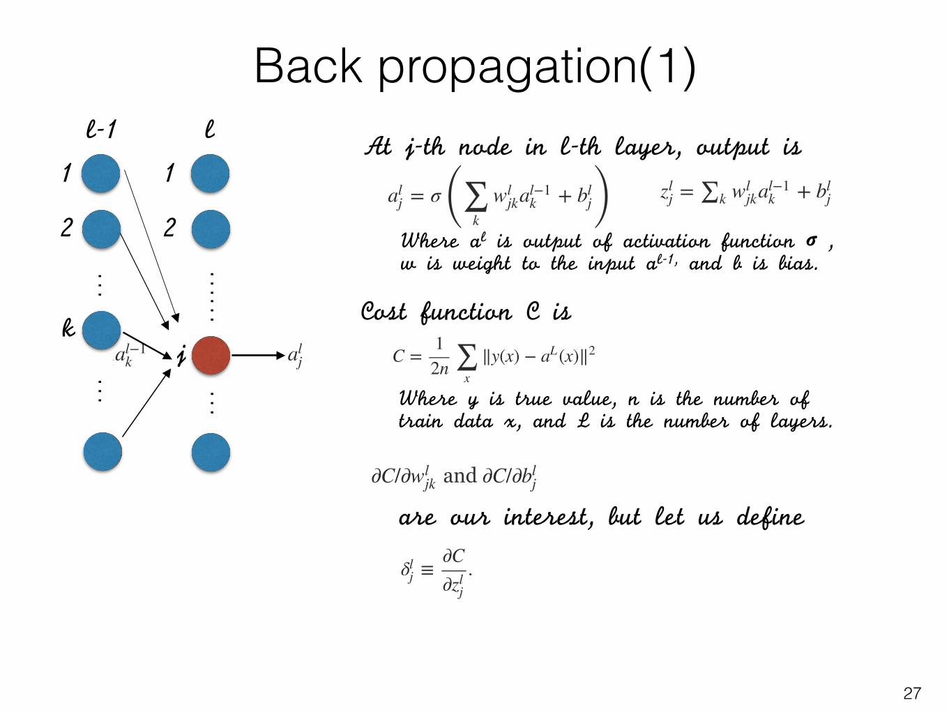
Atj-thnodeinl-thlayer,outputis
And we use for the activation of the neuron in the layer.The following diagram shows examples of these notations in use:
With these notations, the activation of the neuron in the layer is related to the activations in the layer by theequation (compare Equation (4) and surrounding discussion in thelast chapter)
where the sum is over all neurons in the layer. To rewritethis expression in a matrix form we define a weight matrix foreach layer, . The entries of the weight matrix are just the weightsconnecting to the layer of neurons, that is, the entry in the rowand column is . Similarly, for each layer we define a biasvector, . You can probably guess how this works - the componentsof the bias vector are just the values , one component for eachneuron in the layer. And finally, we define an activation vector whose components are the activations .
The last ingredient we need to rewrite (23) in a matrix form is theidea of vectorizing a function such as . We met vectorizationbriefly in the last chapter, but to recap, the idea is that we want toapply a function such as to every element in a vector . We use theobvious notation to denote this kind of elementwise applicationof a function. That is, the components of are just .As an example, if we have the function then the vectorizedform of has the effect
that is, the vectorized just squares every element of the vector.
With these notations in mind, Equation (23) can be rewritten in the
l-1 l
… ……k
j
1
2
1
2
… …
CostfunctionCis
Whereyistruevalue,nisthenumberoftraindatax,andListhenumberoflayers.
beautiful and compact vectorized form
This expression gives us a much more global way of thinking abouthow the activations in one layer relate to activations in the previouslayer: we just apply the weight matrix to the activations, then addthe bias vector, and finally apply the function*. That global view isoften easier and more succinct (and involves fewer indices!) thanthe neuron-by-neuron view we've taken to now. Think of it as a wayof escaping index hell, while remaining precise about what's goingon. The expression is also useful in practice, because most matrixlibraries provide fast ways of implementing matrix multiplication,vector addition, and vectorization. Indeed, the code in the lastchapter made implicit use of this expression to compute thebehaviour of the network.
When using Equation (25) to compute , we compute theintermediate quantity along the way. This quantityturns out to be useful enough to be worth naming: we call theweighted input to the neurons in layer . We'll make considerableuse of the weighted input later in the chapter. Equation (25) issometimes written in terms of the weighted input, as . It'salso worth noting that has components , thatis, is just the weighted input to the activation function for neuron in layer .
The two assumptions we need aboutthe cost functionThe goal of backpropagation is to compute the partial derivatives
and of the cost function with respect to any weight or bias in the network. For backpropagation to work we need tomake two main assumptions about the form of the cost function.Before stating those assumptions, though, it's useful to have anexample cost function in mind. We'll use the quadratic cost functionfrom last chapter (c.f. Equation (6)). In the notation of the lastsection, the quadratic cost has the form
*By the way, it's this expression that motivatesthe quirk in the notation mentioned earlier.
If we used to index the input neuron, and toindex the output neuron, then we'd need toreplace the weight matrix in Equation (25) by thetranspose of the weight matrix. That's a smallchange, but annoying, and we'd lose the easysimplicity of saying (and thinking) "apply theweight matrix to the activations".
Wherealisoutputofactivationfunctionσ,wisweighttotheinputal-1,andbisbias.
The demon sits at the neuron in layer . As the input to theneuron comes in, the demon messes with the neuron's operation. Itadds a little change to the neuron's weighted input, so thatinstead of outputting , the neuron instead outputs .This change propagates through later layers in the network, finallycausing the overall cost to change by an amount .
Now, this demon is a good demon, and is trying to help youimprove the cost, i.e., they're trying to find a which makes thecost smaller. Suppose has a large value (either positive or
negative). Then the demon can lower the cost quite a bit bychoosing to have the opposite sign to . By contrast, if is
close to zero, then the demon can't improve the cost much at all byperturbing the weighted input . So far as the demon can tell, theneuron is already pretty near optimal*. And so there's a heuristicsense in which is a measure of the error in the neuron.
Motivated by this story, we define the error of neuron in layer by
As per our usual conventions, we use to denote the vector oferrors associated with layer . Backpropagation will give us a way ofcomputing for every layer, and then relating those errors to thequantities of real interest, and .
You might wonder why the demon is changing the weighted input . Surely it'd be more natural to imagine the demon changing the
output activation , with the result that we'd be using as our
measure of error. In fact, if you do this things work out quitesimilarly to the discussion below. But it turns out to make thepresentation of backpropagation a little more algebraically
*This is only the case for small changes , ofcourse. We'll assume that the demon isconstrained to make such small changes.
why we're not regarding the cost also as a function of . Remember,
though, that the input training example is fixed, and so the output
is also a fixed parameter. In particular, it's not something we can
modify by changing the weights and biases in any way, i.e., it's not
something which the neural network learns. And so it makes sense
to regard as a function of the output activations alone, with
merely a parameter that helps define that function.
The Hadamard product,
The backpropagation algorithm is based on common linear
algebraic operations - things like vector addition, multiplying a
vector by a matrix, and so on. But one of the operations is a little
less commonly used. In particular, suppose and are two vectors
of the same dimension. Then we use to denote the
elementwise product of the two vectors. Thus the components of
are just . As an example,
This kind of elementwise multiplication is sometimes called the
Hadamard product or Schur product. We'll refer to it as the
Hadamard product. Good matrix libraries usually provide fast
implementations of the Hadamard product, and that comes in
handy when implementing backpropagation.
The four fundamental equations
behind backpropagation
Backpropagation is about understanding how changing the weights
and biases in a network changes the cost function. Ultimately, this
means computing the partial derivatives and . But to
compute those, we first introduce an intermediate quantity, ,
which we call the error in the neuron in the layer.
Backpropagation will give us a procedure to compute the error ,
and then will relate to and .
To understand how the error is defined, imagine there is a demon
in our neural network:
areourinterest,butletusdefine

Back propagation(2)
28
four are consequences of the chain rule from multivariable calculus.
If you're comfortable with the chain rule, then I strongly encourage
you to attempt the derivation yourself before reading on.
Let's begin with Equation (BP1), which gives an expression for the
output error, . To prove this equation, recall that by definition
Applying the chain rule, we can re-express the partial derivative
above in terms of partial derivatives with respect to the output
activations,
where the sum is over all neurons in the output layer. Of course,
the output activation of the neuron depends only on the input
weight for the neuron when . And so vanishes
when . As a result we can simplify the previous equation to
Recalling that the second term on the right can be
written as , and the equation becomes
which is just (BP1), in component form.
Next, we'll prove (BP2), which gives an equation for the error in
terms of the error in the next layer, . To do this, we want to
rewrite in terms of . We can do this using
the chain rule,
where in the last line we have interchanged the two terms on the
right-hand side, and substituted the definition of . To evaluatethe first term on the last line, note that
Differentiating, we obtain
Substituting back into (42) we obtain
This is just (BP2) written in component form.
The final two equations we want to prove are (BP3) and (BP4).These also follow from the chain rule, in a manner similar to theproofs of the two equations above. I leave them to you as anexercise.
Exercise
Prove Equations (BP3) and (BP4).
That completes the proof of the four fundamental equations ofbackpropagation. The proof may seem complicated. But it's reallyjust the outcome of carefully applying the chain rule. A little lesssuccinctly, we can think of backpropagation as a way of computingthe gradient of the cost function by systematically applying thechain rule from multi-variable calculus. That's all there really is tobackpropagation - the rest is details.
The backpropagation algorithmThe backpropagation equations provide us with a way of computingthe gradient of the cost function. Let's explicitly write this out in theform of an algorithm:
1. Input : Set the corresponding activation for the inputlayer.
2. Feedforward: For each compute and .
Fromtheinformationsinl+1-thlayer,wecanobtaintheerrorinl-thlayer.(Backpropagation)
trained, they will still find it extremely difficult to identify the input
image, simply because they don't have enough information. And so
it can't possibly be the case that not much learning needs to be done
in the first layer. If we're going to train deep networks, we need to
figure out how to address the vanishing gradient problem.
What's causing the vanishing gradientproblem? Unstable gradients in deepneural netsTo get insight into why the vanishing gradient problem occurs, let's
consider the simplest deep neural network: one with just a single
neuron in each layer. Here's a network with three hidden layers:
Here, are the weights, are the biases, and is
some cost function. Just to remind you how this works, the output
from the th neuron is , where is the usual sigmoid
activation function, and is the weighted input to the
neuron. I've drawn the cost at the end to emphasize that the cost
is a function of the network's output, : if the actual output from
the network is close to the desired output, then the cost will be low,
while if it's far away, the cost will be high.
We're going to study the gradient associated to the first
hidden neuron. We'll figure out an expression for , and by
studying that expression we'll understand why the vanishing
gradient problem occurs.
I'll start by simply showing you the expression for . It looks
forbidding, but it's actually got a simple structure, which I'll
describe in a moment. Here's the expression (ignore the network,
for now, and note that is just the derivative of the function):
The structure in the expression is as follows: there is a term in
the product for each neuron in the network; a weight term for
In a very simple case( like composed of 4 layers, each has just one node)

29
right-hand side, and substituted the definition of . To evaluatethe first term on the last line, note that
Differentiating, we obtain
Substituting back into (42) we obtain
This is just (BP2) written in component form.
The final two equations we want to prove are (BP3) and (BP4).These also follow from the chain rule, in a manner similar to theproofs of the two equations above. I leave them to you as anexercise.
Exercise
Prove Equations (BP3) and (BP4).
That completes the proof of the four fundamental equations ofbackpropagation. The proof may seem complicated. But it's reallyjust the outcome of carefully applying the chain rule. A little lesssuccinctly, we can think of backpropagation as a way of computingthe gradient of the cost function by systematically applying thechain rule from multi-variable calculus. That's all there really is tobackpropagation - the rest is details.
The backpropagation algorithmThe backpropagation equations provide us with a way of computingthe gradient of the cost function. Let's explicitly write this out in theform of an algorithm:
1. Input : Set the corresponding activation for the inputlayer.
2. Feedforward: For each compute and .
3. Output error : Compute the vector .
4. Backpropagate the error: For each
compute .
5. Output: The gradient of the cost function is given by
and .
Examining the algorithm you can see why it's called
backpropagation. We compute the error vectors backward,
starting from the final layer. It may seem peculiar that we're going
through the network backward. But if you think about the proof of
backpropagation, the backward movement is a consequence of the
fact that the cost is a function of outputs from the network. To
understand how the cost varies with earlier weights and biases we
need to repeatedly apply the chain rule, working backward through
the layers to obtain usable expressions.
Exercises
Backpropagation with a single modified neuron
Suppose we modify a single neuron in a feedforward network
so that the output from the neuron is given by ,
where is some function other than the sigmoid. How should
we modify the backpropagation algorithm in this case?
Backpropagation with linear neurons Suppose we
replace the usual non-linear function with
throughout the network. Rewrite the backpropagation
algorithm for this case.
As I've described it above, the backpropagation algorithm computes
the gradient of the cost function for a single training example,
. In practice, it's common to combine backpropagation with
a learning algorithm such as stochastic gradient descent, in which
we compute the gradient for many training examples. In particular,
given a mini-batch of training examples, the following algorithm
applies a gradient descent learning step based on that mini-batch:
1. Input a set of training examples
2. For each training example : Set the corresponding input
activation , and perform the following steps:
And move w and b in different direction to gradient

21. 11. 2016, MAGIC Collaboration Meeting DortmundKazuma Ishio
Official Performance
30
/ GeVtrueE60 100 200 300 1000 2000 10000 20000
Ener
gy b
ias
and
reso
lutio
n
-0.05
0
0.05
0.1
0.15
0.2
0.25
0.3
0.35)°Bias (2010, < 30 Resolution
)°Bias (2013, < 30 Resolution
) °-45°Bias (2013, 30 Resolution
Figure 10: Energy resolution (solid lines) and bias (dashed lines) obtainedfrom the MC simulations of γ−rays. Events are weighted in order to repre-sent a spectrum with a slope of −2.6. Red: low zenith angle, blue: mediumzenith angle. For comparison, pre-upgrade values from Aleksic et al. (2012a)are shown in gray lines.
15%. For higher energies it degrades due to an increasing frac-tion of truncated images, and showers with high impact param-eters as well as worse statistics in the training sample. Note thatthe energy resolution can be easily improved in the multi-TeVrange with additional quality cuts (e.g. in the maximum recon-structed impact), however at the price of lowering the collectionarea. At low energies the energy resolution is degraded, due toworse precision in the image reconstruction (in particular theimpact parameters), and higher internal relative fluctuations ofthe shower. Above a few hundred GeV the absolute value ofthe bias is below a few percent. At low energies (! 100GeV)the estimated energy bias rapidly increases due to the thresholdeffect. For observations at higher zenith angles the energy res-olution is similar. Since an event of the same energy observedat higher zenith angle will produce a smaller image, the energyresolution at the lowest energies is slightly worse. On the otherhand, at multi-TeV energies, the showers observed at low zenithangle are often partially truncated at the edge of the camera, andmay even saturate some of the pixels (if they produce signals of" 750 phe in single pixels). Therefore the energy resolutionis slightly better for higher zenith angle observations. As theenergy threshold shifts with increasing zenith angle, the energybias at energies below 100 GeV is much stronger for higherzenith angle observations.The distribution (Eest − Etrue)/Etrue is well described by a
Gaussian function in the central region, but not at the edges,where one can appreciate non-Gaussian tails. The energy reso-lution, determined as the sigma of the Gaussian fit, is not verysensitive to these tails. For comparison purposes, we also com-puted the RMS of the distribution (in the range 0 < Eest <2.5 · Etrue), which will naturally be sensitive to the tails of the(Eest − Etrue)/Etrue. The RMS values are reported in TablesA.2 and A.3 for the low and medium zenith angles respectively.While the sigma of the Gaussian fit is in the range 15%-25%,the RMS values lie in the range 20%-30%.
slope2 2.5 3 3.5 4
bias
(mea
n of
Gau
ss)
0
0.05
0.1
0.15
0.2
=0.1 TeVestE
=1 TeVestE
=10 TeVestE
Figure 11: Energy bias as a function of the spectral slope for different estimatedenergies: 0.1TeV (dotted line), 1 TeV (solid), 10 TeV (dashed). Zenith anglebelow 30◦ .
When the data are binned according to estimated energy ofindividual events (note that, in contrary to MC simulations, inthe data only the estimated energy is known) the value of thebias will change depending on the spectral shape of the source.With steeper spectra more events will migrate from lower ener-gies resulting in an overestimation of the energy. Note that thiseffect does not occur in the case of binning the events accordingto their true energy (as in Fig. 10). In Fig. 11 we show such abias as a function of spectral slope for a few values of estimatedenergy. Note that the bias is corrected in the spectral analysisby means of an unfolding procedure (Albert et al., 2007).The energy resolution cannot be checked with the data in
a straight-forward way and one has to rely on the values ob-tained from MC simulations. Nevertheless, we can use thefact of having two, nearly independent estimations of the en-ergy, Eest,1 and Eest,2 from each of the telescopes to performa consistency check. We define relative energy difference asRED = (Eest,1 − Eest,2)/Eest. If the Eest,1 and Eest,2 estima-tors were completely independent the energy resolution wouldbe ≈ RMS (RED)/
√2. In Fig. 12 we show a dependency of
RMS (RED) on the reconstructed energy. The curve obtainedfrom the data is consistent with the one of MC simulationswithin a few percent accuracy. The first point (between 45 and75GeV) shows a sudden drop in RMS (RED) compared to theother points, consistently in the data and MC simulations. Notethat this point is below the analysis threshold, therefore it ismostly composed of peculiar events in which the shower pro-duces more Cherenkov light than average for this energy. Thisresults in a strong correlation of Eest,1 and Eest,2 allowing fora relatively low value of inter-telescope difference in estimatedenergy, and still a rather poor energy resolution.
4.5. Spectrum of the Crab NebulaIn Fig. 13 we show the spectrum of the Crab Nebula obtained
with the total (low + medium zenith angle) sample. For clarity,the spectrum is presented in the form of spectral energy dis-tribution, i.e. E2dN/dE. In order to minimize the systematic
8
Arxiv 1409.5594 The major upgrade of the MAGIC telescopes, Part II: A performance study using observations of the Crab Nebula
My study featuresZd = 05 - 50 deg

31
Energy
Flux
or c
oun
ts
Background