Improved model of a ball bearing forthe simulation of vibration signals dueto faults during run-up

Matej Tadina1, Miha Boltezar1

1Faculty of Mechanical Engineering, University of Ljubljana, Askerceva 6, 1000Ljubljana, SI-Slovenia

Cite as:M. Tadina and M. Boltezar

Improved model of a ball bearing for the simulation of vibration signals dueto faults during run-up. Journal of Sound and Vibration (2011), Volume:

300, Issue 17, Pages 4287-4301

Abstract

In this paper an improved bearing model is developed in order to investigate the vibrations of a ballbearing during run-up. The numerical bearing model was developed with the assumptions that the innerrace has only 2DOF and that the outer race is deformable in the radial direction, and is modelled withfinite elements. The centrifugal load effect and the radial clearance are taken into account. The contactforce for the balls is described by a nonlinear Hertzian contact deformation. Various surface defects dueto local deformations are introduced into the developed model. The detailed geometry of the local defectsis modelled as an impressed ellipsoid on the races and as a flattened sphere for the rolling balls. Withthe developed bearing model the transmission path of the bearing housing can be taken into account,since the outer ring can be coupled with the FE model of the housing. The obtained equations of motionwere solved numerically with a modified Newmark time-integration method for the increasing rotationalfrequency of the shaft. The simulated vibrational response of the bearing with different local faults wasused to test the suitability of the envelope-analysis technique and the continuous wavelet transformationwas used for the bearing fault identification and classification.

1 Introduction

Ball bearings are among the most important and frequently used components the electric motors; howeverbearings may contain manufacturing errors or mounting defects. Damage may also occur during workingconditions. Such errors cause vibration, noise, and even failure of the whole system, which leads toexpensive claims for damage. To avoid this and to ensure rapid and cheap production there is a need fora quick end-test of the electric motors to determine any bearing faults.

The first step in bearing-fault detection during run-up would be a numerical model for the bearing-vibration response due to faults during the run-up. A well-defined vibration signal during the run-upof a faulty bearing could be used to find a suitable method for the fault diagnostic. A lot of researchwork has been done to model the vibration response of a bearing due to faults at a constant rotationalspeed. The early work on the mathematical modelling of localised single and multiple point defects inbearings was published by McFadden and Smith [1,2]. They proposed a vibration model for point defectson the inner race of a rolling-element bearing under a radial load. In this model the vibrations due todefects are modelled as the product of a series of impulses at the rolling-element passing frequency andthe amplitude of the transfer function, convolved with the impulse response of the exponential decay

1

function. A similar analytical model has been proposed by Tandon and Choudhury [3] for predicting thevibration frequencies of rolling bearings and the amplitudes of the significant frequency components dueto localised defects on the outer race, the inner race or on one rolling element under an axial load. Theyextended the model further in [4], where a rotor-bearing system was modelled as a 3 DOF system, and theexcitation force is modelled as periodic pulses [3]. The first mathematical model for modelling bearingvibrations was proposed by Sunnersjo [5]. The bearing was modelled as a 2 DOF system, which providesthe load-deflection according to Hertzian contact theory, while ignoring the mass and the inertia of therolling elements. The two orthogonal DOF are related to the inner race. Rafsanjani et al. [6] combinedthis 2 DOF model with an analytical approach to model the nonlinear dynamic behavior of a bearingdue to localised surface defects. In this model the effect of the radial internal clearance was taken intoaccount. Liew [7] presented four different bearing models in order to model bearing vibrations. The mostcomprehensive model includes the rolling-element centrifugal load, the angular contact and the radialclearance, and is a 5 DOF model. The 5 DOF bearing model includes not only the radial displacementof the inner race, but also the axial displacement and the rotation around the x and y axes, Figure 1.Building on the 2 DOF model developed by Liew, Feng [8] developed a bearing-pedestal model with 4DOF, as it includes a pedestal 2 DOF. The model takes into consideration the slippage in the rollingelements, the effect of mass unbalance in the rotor and the possibility of introducing a localised fault inthe inner or outer race. Arslan and Akturk [9] developed a shaft-bearing system with bearing defects.The model has 3 DOF, 2 DOF for the radial displacement and 1 DOF for the axial displacement. Theballs in the bearing have additional DOFs since they can vibrate in a radial direction. The effect ofthe centrifugal load on the balls is neglected. A new, comprehensive model was proposed by Sopanenand Mikkola [10, 11], which includes the effect of different geometrical faults, such as surface roughness,waviness and localised and distributed defects. The dynamic model is a 6 DOF model, which includesboth the non-linear Hertzian contact deformation and the elasto-hydrodynamic fluid film. The modelof the ball bearing was implemented and analysed using a commercial, multi-body software application(MSC.ADAMS).

Kiral and Karaulle [12] modelled the outer ring and the housing with finite elements and used a radiallydistributed load, as given in [1]. The rotating circumferential load is applied on the nodes whenever aball carrying a load moves over that node. A local defect is modelled by amplifying the magnitudes ofthe radial forces defined for the nodes that are in the defected area.

A common feature of all these models is that the rotational speed of the shaft is constant, the outerring is rigid and is assumed to be firmly fitted to a rigid housing.

Although many researches have investigated the vibration characteristics of ball bearings due to localdefects, no studies have been published on bearing vibration due to local defects during the run-up of theshaft. Hence, this paper will present an improved ball-bearing model with local faults, to simulate thevibration signal of a defective bearing during the run-up of the shaft, where the centrifugal load is takeninto account and the outer ring is deformable in the radial direction. Such a simulated vibration signal ofa faulty bearing will be used to test the suitability of the envelope-analysis technique and wavelet analysisfor bearing-fault identification during run-up.

2 Bearing modelling

Based on previous studies [7, 13–15], a multiple-degree-of-freedom model of a radial ball bearing wasdeveloped, shown in Figure 1, to determine the vibration of a faulty bearing during run-up. The followingassumptions were made:

1. The rolling elements, the inner and outer races and the rotor have motions in the plane of thebearing only.

2. The balls are assumed to have masses, and the vibrations of the balls are considered in the radialdirection. The centrifugal load on the balls is taken onto account.

3. Deformations in the contact occur according to the Hertzian theory of elasticity. The effect of theelastohydrodynamic lubricated (EHL) contact is neglected. The inner ring is rigid. The outer ringis deformable in the radial direction and is modelled with finite elements. The finite elements aretwo-noded, locking-free-shear, curved beam elements, as derived in [16]

2

y

x

koki

curved beamfinite element

nodes

Figure 1: Developed bearing model.

4. The cage is rigid and ensures a constant angular separation between the rolling elements, and hencethere is no interaction between rolling elements. The angular velocity of the cage can change overtime and the velocity of the ball is changing at the same rate.

5. In the bearing model it is assumed that slipping or sliding between the components of the bearingcan occur and this is given by a prescribed function in the bearing model.

6. The rollers in a rolling-element bearing are assumed to have no angular rotation about their axes,i.e. no skewing. Hence, there is no interaction of the corners of the rollers with the cage and theflanges of the races.

7. The bearings are assumed to operate under isothermal conditions. Hence, all thermal effects thatmight arise due to the rise in temperature, such as a change in the lubricant viscosity, the expansionof the rolling elements and the races, and the reducted endurance of the material, are consideredto be absent.

8. The damping of a ball bearing is very small. This damping is present because of friction and a smallamount of lubrication. An estimation of the damping of a ball bearing is very difficult because ofthe dominant extraneous damping, which swamps the damping of the bearing. The damping effectof the EHL contact is neglected. The damping in the proposed model is assumed to be structuraldamping.

9. The outer ring of the bearing is supported by a flexible housing. The housing can have asymmetricstiffness properties. This effect can be described by springs with different stiffness that are con-necting nodes of curved beam elements to the supporting structure or with a finite-element modelof the housing.

2.1 Equation of motion

In the mathematical modelling, the ball bearing is considered as a spring-mass system, where the rollingelements act as nonlinear contact springs and the outer race is a deformable body, as shown in Figure2. Lagrange equations are applied to derive the equations of motion of the bearing model. Using theLagrange equations it is necessary to calculate the total potential and kinetic energy of the system. Inorder to calculate the potential energy of the contact deformation, first the contact deformation of the

3

j − th ball at the inner and outer races has to be calculated. Since the outer race is not fixed and isdeformable in the radial direction, the inner and outer contact deformations are expressed as [14]:

y

x

R( )q

r

ro

roi

ri

rj

cj

qj

qcj

di

dj

rb

Figure 2: Positions of race and balls centres and deflection of the j−th ball-race contact.

δi,j = r + ρb − χj , (1)

δo,j = (ρj + ρb)−R(θj), (2)

The variable θj defines the angular position of the jth ball centre with respect to the centre of theouter race xo and yo, r is the radius of the inner race, ρj is the radial position of the j-th ball, ρb is theradius of the ball, xi and yi are the positions of the inner race, and the position of the centre of the ballfrom the inner race χj is obtained from:

xi + χj cos θχj = xo + ρj cos θj , (3)

yi + χj sin θχj = yo + ρj sin θj , (4)

thus:

χj =((xo − xi)2 + ρ2j + 2ρj(xo − xi) cos(θj) + 2ρj(yo − yi) sin(θj) + (yo − yi)2

)2. (5)

Since the outer ring in the proposed model is deformable, the local radius of the outer race is :

R(θj) = R0 + Nej · de, (6)

where R0 is the radius of the non-deformed outer race, Nej is the vector of the interpolation functions

evaluated at the position in the element where the contact occurs and de is the vector of the nodaldisplacements for the element.

The contact force between the inner race and the ball or the outer race and the ball arise only whenthere is a compression in the contact, which means that δi and δo have to be greater than 0:

δi,j+ =

{r + ρb − χj , if r + ρb − χj > 0

0, otherwise(7)

δo,j+ =

{(ρj + ρb)−R(θj), if (ρj + ρb)−R(θj) > 0

0, otherwise(8)

4

With a known contact deformation and following the procedure described in [17] the total potentialenergy is calculated as:

V = msg(yi + yoi) + Mgdy +mbgNbyo +

Nb∑j=1

mbgρj sin θj +2

5

Nb∑j=1

kiδ52i,j+

+2

5

Nb∑j=1

koδ52o,j+ +

1

2dTKd,

(9)

where ms is the mass of the shaft and the inner ring, M is the mass matrix of the outer ring, dy is thevector of the nodal displacement with non-zero entries only on the y displacements, K is the stiffnessmatrix of the outer ring and the supporting structure, δi,j+ and δo,j+ are the inner and outer deformationof balls, and ki/o is the stiffness coefficient at the inner and outer contacts and it depends on the geometryand the material properties of the contacting surfaces [18].

The bearing’s inner ring has 2 DOFs, and taking into account the deformability of the outer ring, thetotal kinetic energy is thus calculated as:

T =1

2ms(x

2i + y2i ) +

1

2

Nb∑j=1

mb

(ρj

2 + ρ2j θ2j + x2o + y2o + 2xo(− sin θjρj θj + cos θj ρj)

+2yo(cos θjρj θj + sin θj ρj))

+1

2NbIbθ

2j

(1 +

R0

ρb

)2

+1

2Isω

2s +

1

2dTMd,

(10)

where xi, yi are the velocities of the inner race/shaft, ρj is the radial velocity of the j-th roller element,θj is the angular position of the j-th rolling element, mb is the mass of the rolling element, Ib is themoment of inertia of the roller element, Is is the moment of inertia of the shaft and the inner race, ωsis the angular velocity of the shaft, xo, yo are the velocities of the centre of the inner race and d are thenodal velocities of the outer race. It should be noted that xo and yo are not generalized coordinates anddepend on the nodal displacements d and are calculated as:

xo =

∑NN

i=1 dxiNN

, (11)

yo =

∑NN

i=1 dyiNN

, (12)

where NN is the number of nodes of the outer ring and dxi, dyi are the nodal displacements in the x andy directions at node i.

With a known total potential and kinetic energy and by applying the Lagrange equation, the equationsof motion of the inner ring and the rolling elements are derived as:

msxs + ki

N∑j=1

δ32i,j+

ρj cos θj + xo − xiχj

= Fu cos θs (13)

msys + ki

N∑j=1

δ32i,j+

ρj sin θj + yo − yiχj

= msg + Fu sin θs (14)

mbρj − ρjω2 + koδ32o,j+ − kiδ

32i,j

ρ+ (xo − xi) cos θj + (yo − yi) sin θjχj

=

−mbg sin θj −mb(xo cos θj + yo sin θj)

(15)

And for the outer ring, since the finite elements are used:

Md + Cd + Kd = Fm (16)

where M is the structural mass matrix, K is the structural stiffness matrix and Fm are the nodal forcesin the finite-element model and d is the displacement vector, and dot notation is used to denote thedifferentiation with respect to time. C is the structural damping matrix, which is additionally introducedas the equivalent Rayleigh damping:

C = αM + βK (17)

5

Because the location of the contact forces between the outer ring and the rolling element moves onthe beam element, the moving load formulation within the element has to be used. The moving loadvector Fm for the outer ring is formulated as:

Fm =

N∑j=1

NTj Fo,j , (18)

where NTj is the transposed vector of the interpolation functions, Fo,j is the contact force on the outer

race at the j-th ball. Using the equations (2) and (6) the outer contact force at the j-th ball can bewritten as:

Fo,j = ko (ρj + ρb − (R0 + Njd))32 , (19)

where Nj is the vector of the shape functions evaluated at the position of the ball’s outer-race contact.It should be noted that Nj is a vector with zero entries, except those corresponding to the curved beamnodal displacement on which the contact of the j-th ball occurs. Thus for a curved beam element with sixdegrees of freedom, the number of non-zero entries within a 1× n vector will be six, where n is the totaldegrees of freedom in the finite+element model of the outer race. The values of this 1× 6 subvector aredependent on the application point of the contact within an element. Since the loads in the finite-elementmodel can be applied only at nodes, the point contact force must be reduced to the equivalent nodalforces and moments. When the contact point moves to another position, the numerical values of theinterpolation functions change, and consequently, the equivalent nodal loads vary accordingly. It shouldbe apparent that when the contact point moves to an adjacent element the interpolation functions of thenew element must be used.

The equations (13)-(16) are nonlinear, coupled, ordinary differential equations and a modified, explicitNewmark method can be used to solve them.

3 Modelling of faults

At an early stage of the bearing’s operation almost only local defects are present due to the impropermounting of the bearing, which will cause a dent due to the plastic deformation of the rolling surface.Another local defect may be present in the bearing due to debris, since grease in the bearing can containparticle contaminants. Such particle contaminant can be modelled as a local defect with the exceptionthat the particle is free to move within the bearing. Most of the presented models of bearing faults [6,8,9]assume that the rolling element will lose contact suddenly once it enters the dent region, and will regaincontact instantly when exiting that area. In this way the modelling results in very large impulsiveforces in the system and as a consequence the acceleration increases sharply in order to maintain thebalance within system. In order to model the behaviour of the rolling element so as to reflect the actualpath that the rolling element takes while rolling into and out of the dent, the dent was modelled as anellipsoidal depression on the inner and outer races, while the dent on the rolling element was modelled asa flattened sphere. Another important aspect of this model is that due to the different geometry of thecontact between the dent and the bearing component the contact-stiffness changes due to the differentgeometrical properties in the contact.

3.1 Outer-race defect

Let there be a defect on the surface of the outer race at an angle ϕ from the horizontal axis, as shownin Figure 3. The dent has an angle length of ϕd. If the rolling-element position θj coincides with thedent-angle range ϕ < θj < ϕ+ ϕD the contact deformation will be smaller for the dent depth Dd at theposition ϕc where is the contact point C. The contact deformation between the rolling element and thedent is now calculated as:

δDo+ =

{‖ρj + ρbC‖ − (R(ϕC) +Ddo(ϕC)) if ‖ρj + ρbC‖ − (R(ϕC) +Dd(ϕC)) > 0

0, otherwise(20)

where Dd is the depth of the dent at the contact position ϕc. It should be noted that the contactdeformation in the dent is given by simple equation (20), although behind these equations are hidden

6

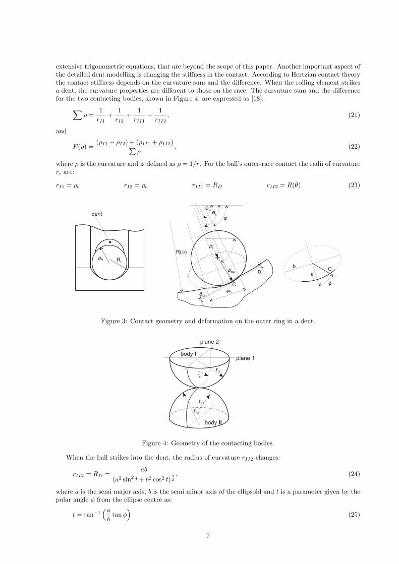
extensive trigonometric equations, that are beyond the scope of this paper. Another important aspect ofthe detailed dent modelling is changing the stiffness in the contact. According to Hertzian contact theorythe contact stiffness depends on the curvature sum and the difference. When the rolling element strikesa dent, the curvature properties are different to those on the race. The curvature sum and the differencefor the two contacting bodies, shown in Figure 4, are expressed as [18]:∑

ρ =1

rI1+

1

rI2+

1

rII1+

1

rII2, (21)

and

F (ρ) =(ρI1 − ρI2) + (ρII1 + ρII2)∑

ρ, (22)

where ρ is the curvature and is defined as ρ = 1/r. For the ball’s outer-race contact the radii of curvatureri are:

rI1 = ρb rI2 = ρb rII1 = RD rII2 = R(θ) (23)

f

qj

jDdDi

qC

rbC

rb

rj

j

a

b

R( )q

Dd

C

C

Rr

dent

Figure 3: Contact geometry and deformation on the outer ring in a dent.

rI1

rII1

rII2

rI2

body I

body II

plane 1

plane 2

Figure 4: Geometry of the contacting bodies.

When the ball strikes into the dent, the radius of curvature rII2 changes:

rII2 = RD =ab

(a2 sin2 t+ b2 cos2 t)32

, (24)

where a is the semi major axis, b is the semi minor axis of the ellipsoid and t is a parameter given by thepolar angle φ from the ellipse centre as:

t = tan−1(ab

tanφ)

(25)

7

Although the radius of curvature RII1 should change, it is assumed that the change of this radius isnegligible in order to avoid problems during the transition from the race into the dent. With the knownsum and curvature difference the contact stiffness kd,o in the dent can be calculated according to Hertziantheory. From equation (24) it is clear that the contact stiffness is a continuous function of the angle φ.Figure 3 shows that the contact force does not act in the direction of ρj under the angle θj but underthe angle θC , and thus the contact force in the radial direction is:

Fc,d = kd,oδ32

Do+ cos(θj − θC) (26)

The tangential component of the contact force in the dent is neglected because the cage ensures theangular position of the rolling elements, but is taken into account as the loading on the outer race.

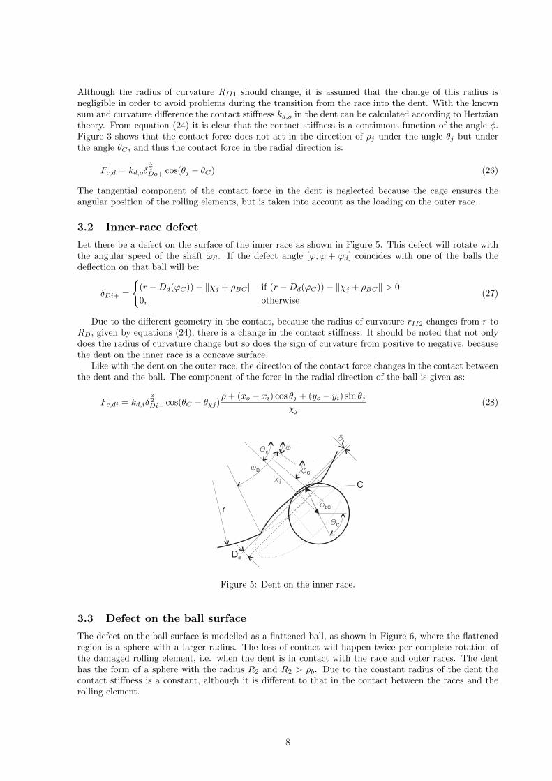
3.2 Inner-race defect

Let there be a defect on the surface of the inner race as shown in Figure 5. This defect will rotate withthe angular speed of the shaft ωS . If the defect angle [ϕ,ϕ + ϕd] coincides with one of the balls thedeflection on that ball will be:

δDi+ =

{(r −Dd(ϕC))− ‖χj + ρBC‖ if (r −Dd(ϕC))− ‖χj + ρBC‖ > 0

0, otherwise(27)

Due to the different geometry in the contact, because the radius of curvature rII2 changes from r toRD, given by equations (24), there is a change in the contact stiffness. It should be noted that not onlydoes the radius of curvature change but so does the sign of curvature from positive to negative, becausethe dent on the inner race is a concave surface.

Like with the dent on the outer race, the direction of the contact force changes in the contact betweenthe dent and the ball. The component of the force in the radial direction of the ball is given as:

Fc,di = kd,iδ32

Di+ cos(θC − θχj)ρ+ (xo − xi) cos θj + (yo − yi) sin θj

χj(28)

C

dd

r

Dd

qx

qC

cj

rbC

jD

j

jC

d

Figure 5: Dent on the inner race.

3.3 Defect on the ball surface

The defect on the ball surface is modelled as a flattened ball, as shown in Figure 6, where the flattenedregion is a sphere with a larger radius. The loss of contact will happen twice per complete rotation ofthe damaged rolling element, i.e. when the dent is in contact with the race and outer races. The denthas the form of a sphere with the radius R2 and R2 > ρb. Due to the constant radius of the dent thecontact stiffness is a constant, although it is different to that in the contact between the races and therolling element.

8

qcj

cj

rB

j

jD

fCr

12

r

R2

rj

qj

rB

j

jDfC

r12

R2

R( )q

Figure 6: Dent on the rolling element. (a) Contact between the inner race and the dent on the ballsurface. (b) Contact between the outer race and the dent on the ball surface.

When the dent of the rolling element is in contact with the inner ring, the contact deformation isdefined as:

δDBi =

{r − (‖χj + ρ12‖ −R2), if r − ‖χj + ρ12‖+R2 > 0

0, else(29)

where ρ12 is the vector from the centre of the rolling element to the centre of the radii of the flattenedcurvature. The projection of the contact force to the radial direction of the rolling element is:

FDCi = kDCiδ32

DBi

ρ+ (xo − xi) cos θj + (yo − yi) sin θjχj

cos(θx − φC), (30)

where kDCi is the contact stiffness between the dent and the inner race. The radii of curvature for therolling element that are taken into account to calculate the contact stiffness are:

rI1 = ρb rI2 = ρb (31)

The contact deformation between the dent and the outer race is given by:

δDBo =

{‖ρj + ρ12‖+R2 −R(θ), if ‖ρj + ρ12‖+R2 −R(θ) > 0

0, else(32)

and the contact force in the radial direction of the ball position is given by:

FDCo = kDCoδ32

DBo

ρ+ (xo − xi) cos θj + (yo − yi) sin θjχj

cos(θj − φC) (33)

4 Numerical results

In this section the presented model was used to simulate the vibration response of a bearing with differentfaults during run-up. Whenever the fault is in contact with its mating surface, one of the equations (26)-(33) is used to replace the appropriate equations for the contact force in equations (13)-(16).

The bearing under investigation is NMB R-1240KK1, shown in Figure 7(a), whose parameters aregiven in Table 1. The outer ring is assumed to be closely fitted into another aluminium ring, whichrepresents the housing of the bearing and the under half of the aluminium ring is connected with springsto the fixed pedestal, as shown in Figure 7(b). The aluminium ring is 3mm thick, and is connectedwith 36 linear springs to the fixed pedestal. The stiffness of the connecting spring is ks = 100000 N/m.In the analysed case a simple support structure was chosen to avoid confusing the bearing vibrationwith the structural vibration, since the transfer path of the housing could change the vibration signal.The outer ring of the bearing and the aluminium ring is modelled with 72 finite elements. The bearingloads are assumed to be the gravitational load and the unbalanced force. The unbalance of the rotor ismeu = 2×10−5 kgm2. From the radius of the inner and outer races it is clear that the radial clearance in

9

Table 1: Geometrical and physical properties used for the rolling-element bearing shown in Figure7(a).Inner-race radius r 2.754 mmOuter-race radius R 4.7565 mmBall radius ρb 1 mmInner-race radius curvature rII1i 1.04 mmOuter-race radius curvature rII1o 1.07 mmArea of outer race AoR 5.37mm2

Principal moment of inertia of outer race IoR 0.888 mm4

Radius to the centre of outer race RC 5.314 mmNumber of balls Nb 7Ball mass mb 0.0000329 kgMass of inner ring and shaft mS 0.15 kgRadial clearance c 5 µmInner contact stiffness ki 3.828× 109 N/mOuter contact stiffness ko 3.867× 109 N/m

rII1o

rII1i

rRRC

rB

AOR IOR

(a) Geometrical properties of the bear-ing.

aluminumring

P1

(b) Analysed bearing-pedestal structure.

Figure 7: Analysed bearing during run up.

0.8

0.2

0.015r

(a) Inner race.

0.75

0.0150.41

R

(b) Outer race.

46O

r 2

0.01

(c) Ball.

Figure 8: Dent geometry on different bearing components.

the bearing is c = 5 µm. The outer ring, the inner ring and the shaft are made from steel. The dynamicresponse of the bearing will be taken from point P1, which is on the top of the aluminium ring, Figure7(b).

The geometrical properties of the local faults are shown in Figure 8. The faults on the inner race andthe ball will rotate and their position will move in and out of the loading zone in the bearing. The faulton the outer race is stationary, and the position of the dent on outer race is very important. Analyseswill be made for the dent in the middle of the loading zone, at the bottom of the outer race.

10

4.1 Initial condition and numerical solution

For the numerical solution the initial conditions and the step size are very important for a successful andeconomical computational solution. The larger the time step, the faster the computation. On other hand,the time step should be small enough to achieve an adequate accuracy. Due to the very high contactstiffness k ≈ 4× 109 N/m, and the very high eigenfrequncies of the outer ring, the first eigenfrequency isat f1 ≈ 35 kHz, and the time step in the presented simulation is δt = 1.5×10−8 s. Since the time step hasto be very small so that the explicit Newmark method is stable, the following strategy was used. First,the initial conditions for the following simulation were calculated, where the shaft was held at centre andwas released to calculate the equilibrium position of the whole system due to the gravitational load. Thiscalculated equilibrium position will be used in the following simulations to avoid passing the transientvibration due to the release of the shaft from centre, and the shaft can start accelerating immediately.

4.2 Vibration response of the bearing due to local faults during the run-upof the shaft

With the presented model, the vibration response of the roller-element bearing due to a local defect issimulated during the run-up of the shaft. The rotational speed of the shaft ωS increases linearly with time.The angular acceleration of the shaft is set to αS = 20π rad/s2. The vibration signals will be processed inthe frequency and time-frequency domains. The basic indicator in the frequency domain is the presenceof the characteristic defect frequencies. The characteristic defect frequencies depend on the rotationalspeed of the shaft and the location of the defect in the bearing. The expressions for the characteristicdefect frequencies for the various defect locations are well established [19]. The characteristic defectfrequencies for the analysed bearing are listed in Table 2, where fS is the rotational speed of the shaft,and fb is the ball’s rotational frequency. In the analysed cases the rotational speed of the shaft fS willbe increasing from 0 to 45 Hz.

Table 2: Characteristic defect frequencies for the stationary outer ring.Outer race defect frequency, foD 2.568fSInner race defect frequency, fiD 4.432fSBall defect frequency, fbD = 2fb 3.488fS

In the frequency domain the demodulation or enveloping-based methods offer the greatest reliablediagnostic potential at a constant rotational speed of the shaft. Although the rotational speed of theshaft will change with time, the method will be tested for bearing-fault detection. The general assumptionwith the enveloping approach is that a measured signal contains low-frequency phenomena that act asthe modulator to the high-frequency carrier signal. For the bearing fault, the low-frequency phenomenonis the impact caused by the defect in the bearing; the high frequency is a combination of the naturalfrequencies of the associated bearing and the surrounding structure of the bearing. The goal of envelopingis to replace the high-frequency oscillation caused by the impact with a single pulse over the entire durationof the impact response. There are several demodulation methods, but the most widely used and well-established of these is the Hilbert transform. Fourier transformation assumes that the signal is periodic,but this is not true due to the changing angular velocity of the shaft, which has the consequence that theoccurrence of the impact is never reproduced exactly from one cycle to another. To minimise this effect,only a short period of the damaged bearing signal will be taken for the analysis. The consequence will bethat the signal has to be zero padded to increase the frequency domain resolution. However, frequency-based techniques are not suitable for the analysis of non-stationary signals that are generally related tothe bearing fault, especially during run-up. Non-stationary signals can be analysed by applying time-frequency domain techniques such as the short-time Fourier transform, the Wavelet transform (WT) andthe Hilbert-Huang transform [20, 21]. In fault diagnostics, the WT is the most popular time-frequencydomain technique, because it can provide a more flexible, multi-resolution solution than the short-timeFT. According to the signal decomposition paradigm, the WT can be classified as the continuous WT(CWT), the discrete WT (DWT) and wavelet packet analysis. For the detection of the present bearingfault the CWT transform will be used. The damaged bearing will produce small amplitudes of vibrationin the high frequency band as the response of the bearing and the housing to the impact that is caused bythe fault. This high-frequency band has to be known prior to the wavelet analysis. In the analysed case,Figure 7(b), the high-frequency response will be at the eigenfrequency of the bearing/housing-pedestal

11

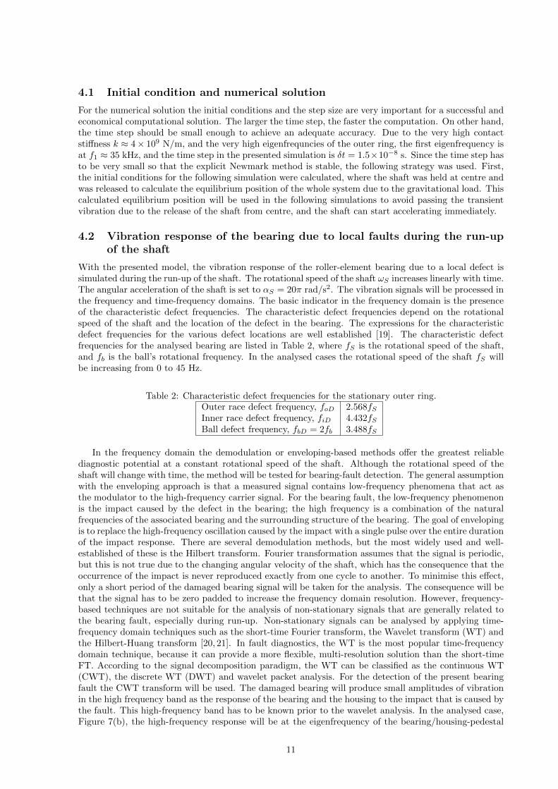
system, which is around 8.2 kHz; the eigenfrequency of the shaft is around 11.3 kHz, although thisfrequency varies due to the changing position of the balls, and the first eigenfrequency of the outer ringwith the aluminium ring is around 36 kHz. The existence of vibrations in these frequency bands will beused to identify the bearing faults. The classification of the bearing faults will be made based on thetime interval between the repetitive vibrations in the high-frequency band. The time interval betweenthe vibrations in the high-frequency band is determined by the instantaneous rotational frequency of theshaft and the type of bearing fault.

All the envelope analyses will be made for the time signal between 2.3 s and 2.4 s. The angular speedof the shaft during this period of time will linearly change from 21 Hz to 22Hz. The CWT analysis willbe made for the time signal between 2.2 s and 2.5 s, and the rotational speed of the shaft is linearlychanging from 20 Hz to 23 Hz. The vibration signal was filtered with a high-pass Butterworth filter,where the cutoff frequency was set to 5 kHz.

4.2.1 Healthy bearing

Bearing components generate vibration signals that are related to the speed of the shaft’s rotation, whichis changing. Figure 9(a) shows the acceleration response at the point P1. It can be seen that even aperfect bearing will generate vibrations due to the time-varying distribution of the balls relative to theinner and outer races. Figure 9(b) shows the vibration spectrum of the envelope analysis. The are twodominant frequency peaks, one at 21 Hz, which is equal to the frequency of the shaft rotation, and theother at 78 Hz, which is the characteristic defect frequency of the ball.

2.2 2.3 2.4 2.5 2.6 2.7 2.8−4

−2

0

2

4

6

Acc

eler

atio

n [m

/s2 ]

Time [s]

(a)

50 100 150 200 250 3000

5

10

15

20

25

Pow

er

spectr

um

Frequency [Hz]

2178

(b)

Figure 9: Vibration response of a healthy bearing. (a) Vibration response at point P1. (b) Frequencyspectrum of the envelope between 2.3 s and 2.4 s.

The time-frequency plot of the CWT is shown in Figure 10. There are small amplitudes of thevibration in the high-frequency band, most of them around 11 kHz. The time intervals T1 ≈ 0.0125 sand T2 ≈ 0.0099 s between two consecutive amplitudes indicate the excitation at a high frequency. Thetime interval T1 corresponds to the frequency f1 = 85.5 Hz, which is the 4th harmonic of the shaft’sinstantaneous rotating frequency, which is at t = 2.24 s fS1 = 20.3 Hz. The time interval T2 correspondsfrequency to the f2 = 101 Hz, which would indicate bearing inner-race damage, since the characteristicinner-race defect frequency at an instantaneous shaft speed fSi = 22.2 Hz is fiD = 4.432 × 22.3 = 98.8Hz. Although the bearing is healthy, there is the presence of the characteristic frequency of the innerrace fault. This presence is due to the varying position of balls in the bearing and due to the centrifugalloading of the shaft. From the time signal it is clear that the amplitude of the bearing vibration isvery small. The conclusion can be made that the bearing has no fault, although in the spectra thereare detectable characteristic fault frequencies. If the bearing was faulty, there would also be a secondharmonic of the characteristic fault frequency.

12

Time [s]

Fre

quency [H

z]

2.2 2.25 2.3 2.35 2.4 2.45 2.50.5

1

1.5

2

2.5

3

3.5

4x 10

4

0

0.01

0.02

0.03

0.04

0.05

0.06

0.07

0.08

T1

T2

Figure 10: Time-frequency plot of the CWT of the bearing vibration signal in healthy case.

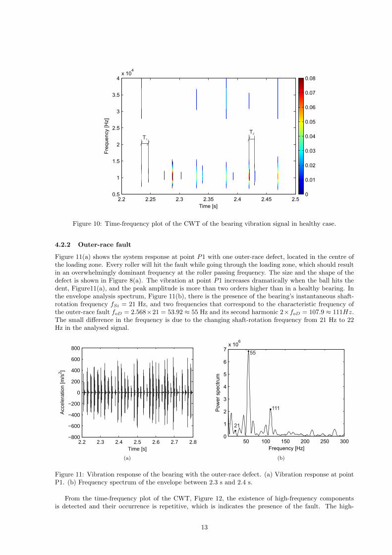
4.2.2 Outer-race fault

Figure 11(a) shows the system response at point P1 with one outer-race defect, located in the centre ofthe loading zone. Every roller will hit the fault while going through the loading zone, which should resultin an overwhelmingly dominant frequency at the roller passing frequency. The size and the shape of thedefect is shown in Figure 8(a). The vibration at point P1 increases dramatically when the ball hits thedent, Figure11(a), and the peak amplitude is more than two orders higher than in a healthy bearing. Inthe envelope analysis spectrum, Figure 11(b), there is the presence of the bearing’s instantaneous shaft-rotation frequency fSi = 21 Hz, and two frequencies that correspond to the characteristic frequency ofthe outer-race fault foD = 2.568×21 = 53.92 ≈ 55 Hz and its second harmonic 2×foD = 107.9 ≈ 111Hz.The small difference in the frequency is due to the changing shaft-rotation frequency from 21 Hz to 22Hz in the analysed signal.

2.2 2.3 2.4 2.5 2.6 2.7 2.8−800

−600

−400

−200

0

200

400

600

800

Acc

eler

atio

n [m

/s2 ]

Time [s]

(a)

50 100 150 200 250 3000

1

2

3

4

5

6

7x 10

6

Pow

er

spectr

um

Frequency [Hz]

21

55

111

(b)

Figure 11: Vibration response of the bearing with the outer-race defect. (a) Vibration response at pointP1. (b) Frequency spectrum of the envelope between 2.3 s and 2.4 s.

From the time-frequency plot of the CWT, Figure 12, the existence of high-frequency componentsis detected and their occurrence is repetitive, which is indicates the presence of the fault. The high-

13

frequency response is observed at the first eigenfrequency of the outer race and the eigenfrequency of theouter ring-pedestal system, which is higher in amplitude. The time intervals T1 = 0.019 s and T2 = 0.0179s correspond to the frequencies f1 = 52.6 Hz and f2 = 55.9 Hz. These two frequencies are correlated withthe characteristic frequencies of the outer-race defect, at the shaft’s instantaneous rotational frequenciesfSi1 = 20.7 Hz and fSi2 = 21.5 Hz.

Time [s]

Fre

quency [H

z]

2.2 2.25 2.3 2.35 2.4 2.45 2.50.5

1

1.5

2

2.5

3

3.5

4x 10

4

0.5

1

1.5

2

2.5x 10

-3

T1

T2

Figure 12: Time-frequency plot of the CWT of the bearing vibration signal with the outer-race fault.

It is clear that each technique can detect the presence of this bearing fault.

4.2.3 Inner-race fault

The defect on the inner race will rotate with the shaft’s rotation speed and will go through the loadingzone every cycle. The response will be very high when the defect it hits its mating surface in the loadingzone On the other hand, when the defect will be on top the balls it will mostly miss the point defect,and thus shift the dominant faulty frequency to lower bands. For this reason the detection of a fault onthe inner race is more challenging than on a fixed race. Figure 13(a) shows the vibration response of theouter ring to the inner-race defect. The size and the shape of the inner-race defect are shown in Figure8(b).

The envelope spectrum shows a shaft frequency peak at 22 Hz, which is the shaft’s rotating frequency.The characteristic frequency of the inner race defect fiD = 4.432× 22 = 97.5 Hz and its second harmonic2× fiD = 195 Hz can be clearly identified in the envelope spectrum, Figure 13(b). The small differencein the frequencies is due to the changing speed of the shaft.

From the time-frequency plot of the CWT, Figure 14, the existence of high-frequency components isdetected and their occurrence is repetitive, which indicates the presence of the fault. The vibrations ofthe bearing/pedestal structure appear in the spectrum only when the inner-race fault is in the loadingzone. Due to this the interval between two consecutive components of the vibration in the high-frequencyband has to be carefully chosen. The time intervals T1 = 0.0108 s and T2 = 0.0102 s correspondto the frequencies f1 = 92.6 HZ and f2 = 98.3Hz. These two frequencies correlate very well withthe characteristic frequencies of the outer-race defect at the instantaneous shaft speeds fSi1 = 20.7 att1 = 2.27 s and fSi2 = 22.5 Hz at t2 = 2.45 s.

It is clear that each technique can detect the presence of this bearing fault, where the time interval inthe CWT has to be taken carefully, since only in the loading zone is there the high frequency vibration.

4.2.4 Rolling-element fault

To investigate the vibration response of the bearing to the ball fault, it is assumed that the dent is onthe 1st ball. The size and the geometry of the flattened ball are shown in Figure 8(c). The vibration

14

2.2 2.3 2.4 2.5 2.6 2.7 2.8−1000

−500

0

500

1000

1500

Acc

eler

atio

n [m

/s2 ]

Time [s]

(a)

50 100 150 200 250 3000

0.5

1

1.5

2

2.5

3x 10

6

Pow

er

spectr

um

Frequency [Hz]

22

95

191

(b)

Figure 13: Vibration response of the bearing with the inner-race defect. (a) Vibration response at pointP1. (b) Frequency spectrum of the envelope between 2.3 s and 2.4 s.

Time [s]

Fre

quency [H

z]

2.2 2.25 2.3 2.35 2.4 2.45 2.50.5

1

1.5

2

2.5

3

3.5

4x 10

4

0

0.5

1

1.5

2

2.5

3x 10

-3

T1

T2

Figure 14: Time-frequency plot of the CWT of the bearing vibration signal with the inner-race fault.

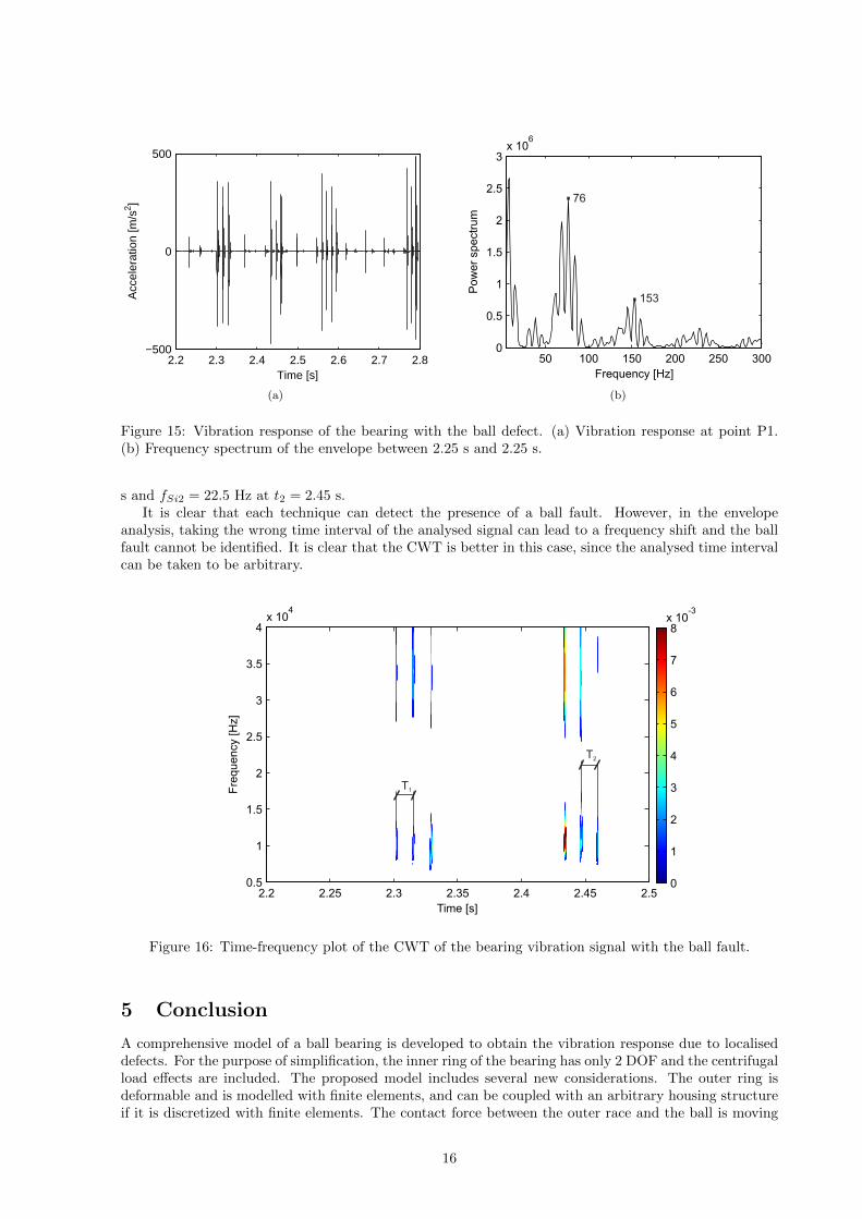
response at point P1 is shown in Figure 15(a). The vibration signal is highly modulated, since the highimpulsive response is noticed only when the damaged ball is in the loading zone. For this reason the signaltaken for the envelope analysis has to be taken carefully. For the spectrum of the envelope analysis thevibration signal is taken from 2.3 s to 2.45 s. With the shorter signal the characteristic defect frequencyit hard to identify, but due to a larger change of the shaft’s rotation frequency in this time interval, theshaft’s rotation frequency is not present in the frequency spectrum of the envelope analysis. From thesimulation it is known that the shaft’s rotation frequency increases from 21 Hz to 22.5 Hz. However, thecharacteristic defect frequency of the ball defect fbD = 3.488 × 21.5 = 75 Hz and its second harmonic2× fbD = 150 Hz can be identified clearly in the envelope-analysis spectrum Figure 15(b).

From the time-frequency plot of the CWT the existence of high-frequency components is detectedonly when the ball is in the load zone. The time interval between two consecutive amplitudes in thehigh-frequency band determines the presence of the ball faults. The time intervals T1 = 0.0134 s andT2 = 0.0125 s correspond to the frequencies f1 = 74.6 Hz and f2 = 80 Hz, which are characteristicfrequencies of the ball defect at the shaft’s instantaneous rotational frequencies fSi1 = 21 Hz at t1 = 2.3

15

2.2 2.3 2.4 2.5 2.6 2.7 2.8−500

0

500

Acc

eler

atio

n [m

/s2 ]

Time [s]

(a)

50 100 150 200 250 3000

0.5

1

1.5

2

2.5

3x 10

6

Pow

er

spectr

um

Frequency [Hz]

76

153

(b)

Figure 15: Vibration response of the bearing with the ball defect. (a) Vibration response at point P1.(b) Frequency spectrum of the envelope between 2.25 s and 2.25 s.

s and fSi2 = 22.5 Hz at t2 = 2.45 s.It is clear that each technique can detect the presence of a ball fault. However, in the envelope

analysis, taking the wrong time interval of the analysed signal can lead to a frequency shift and the ballfault cannot be identified. It is clear that the CWT is better in this case, since the analysed time intervalcan be taken to be arbitrary.

Time [s]

Fre

quency [H

z]

2.2 2.25 2.3 2.35 2.4 2.45 2.50.5

1

1.5

2

2.5

3

3.5

4x 10

4

0

1

2

3

4

5

6

7

8x 10

-3

T1

T2

Figure 16: Time-frequency plot of the CWT of the bearing vibration signal with the ball fault.

5 Conclusion

A comprehensive model of a ball bearing is developed to obtain the vibration response due to localiseddefects. For the purpose of simplification, the inner ring of the bearing has only 2 DOF and the centrifugalload effects are included. The proposed model includes several new considerations. The outer ring isdeformable and is modelled with finite elements, and can be coupled with an arbitrary housing structureif it is discretized with finite elements. The contact force between the outer race and the ball is moving

16

within the finite element continuously, and due to this the finite element can be larger and the finalmodel is computationally less demanding. The contact properties are described with detailed geometricalproperties and small changes in the contact stiffness are taken into account.

The developed bearing model is used to simulate the vibration response of the bearing/pedestal systemdue to different local faults, while the shaft’s rotational frequency is increasing. Although the rotationalfrequency is non-stationary, the envelope analysis method could identify all the local bearing defects.The time interval for the envelope analysis has to be taken carefully, since the defect on the bearingelement has to be in the loading zone in that time interval, but the time interval has to be short enoughso that there is only a small change in the shaft’s rotating frequency. The signal used for the envelopeanalysis has to be zero padded to have a sufficient frequency resolution, where we have to be aware of thelimitations and consequences of zero padding. On other hand, the CWT gives the same results, wherethe analysed time interval can be taken as arbitrary to identify the bearing faults.

References

[1] P.D. McFadden and J.D. Smith. Model for the vibration produced by a single point defect in arolling element bearing. Journal of Sound and Vibration, 96:69–82, 1984.

[2] P.D. McFadden and J.D. Smith. The vibration produced by multiple point defect in a rolling elementbearing. Journal of Sound and Vibration, 98:263–273, 1985.

[3] N. Tandodn and A. Choudhury. An analytical model for the prediction of the vibrations responseof rolling element bearings due to a localized defect. Journal of Sound and Vibration, 205:275–292,1997.

[4] A. Choudhury and N. Tandon. Vibration response of rolling element bearings in a rotor system toa local defects under radial load. Journal of Tribology, 128:251–261, 2006.

[5] C.S. Sunnersjo. Varying compliance vibrations of rolling element bearings. Journal of Sound andVibration, 3:363–373, 1978.

[6] A. Rafsanjani, S. Abbasion, A. Farshidianfar, and H. Moeenfard. Nonlinear dynamic modeling ofsurface defects in rolling element bearing systems. Journal of Sound and Vibration, 319:1150–1174,2009.

[7] A. Liew, N.Feng, and E.J. Hahn. Transient rotor dynamic modelling of rolling element bearingsystems. ASME Journal of Engineering for Gas Turbines and Power, 124:984–991, 2002.

[8] N. S. Feng, E. J. Hahn, and R. B. Randall. Using transient analysis software to simulate vibrationssignals due to rolling element bearing defects. Proceedings of the 3rd Australian Congress on AppliedMEchanics, pages 689–694, 2002.

[9] H. Arslan and N. Akturk. An investigation of rolling element vibrations caused by local defects.Journal of Tribology, 130, 2008.

[10] J. Sopanen and A. Mikola. Dynamic model of a deep-groove ball bearing including localized and dis-tributed defects—part 1: theory. Proceedings of the Institution of Mechanical Engineers K—Journalof Multi-body Dynamics, 217:201–211, 2003.

[11] J. Sopanen and A. Mikola. Dynamic model of a deep-groove ball bearing including localized anddistributed defects—part 2: implementation and results. Proceedings of the Institution of MechanicalEngineers K—Journal Multi-body Dynamics, 217:213–223, 2003.

[12] Z. Kiral and H. Karagulle. Simulation and analysis of vibration signals generated by rolling elementbearing with defects. Tribology International, 36:667–678, 2003.

[13] S.P. Harsha. The effect of ball size variation on nonlinear vibrations associated with ball bearings.Proceedings of the Institution of Mechanical Engineers, Part K: Journal of Multi-body Dynamics,218:191–210, 2004.

17

[14] S.P. Harsha. Nonlinear dynamic analysis of rolling element bearings due to cage run-out and numberof balls. Journal of Sound and Vibration, 289:360–381, 2006.

[15] M. Cao and J. Xiao. A comprehensive dynamic model of double-row spherical roller bearing-modeldevelopment and case studies on surface defects, preloads, and radial clearance. Mechanical Systemsand Signal Processing, 22:467–489, 2008.

[16] P. Raveendranathh, G. Singh, and B. Pradhan. A two-noded locking-free shear flexible curved beamelement. Int. J. for Numerical Methods in Engineering, 44:265–280, 1999.

[17] S.P. Harsha. Nonlinear dynamic analysis of an unbalanced rotor supported by roller bearing. Chaos,Solitions and Fractals, 26:47–66, 2005.

[18] T. A. Harris. Rolling bearing analysis. John Wiley and Sons, 2001.

[19] N. Tandon and A. Choudhury. A review of vibration and acoustic measurement methods for thedetection of defects in rolling element bearings. Tribology International, 32:469–480, 1999.

[20] R.X. Gao and R. Yan. Non-stationary signal processing for bearing health monitoring. InternationalJournal of Manufacturing Research, 1:18–40, 2006.

[21] T. Kijewski-Correa and A. Kareem. Efficacy of Hilbert and wavelet transforms for time-frequencyanalysis. Journal of Engineering Mechanics, pages 1037–1049, 2006.

18