improved ilrs modeling: vlbi-slr scale difference 0.23 ppb

Improved ILRS Modeling: VLBI-SLR Scale Difference ～0.23 ppb

• The systematic re-analysis of LAGEOS-1 & 2 and Etalon 1 & 2 data (1993-2019) produced a preliminary set of persistent long-term biases at the most active SLR stations.

• When these biases are implemented in the reprocessing for the development of the SLR contribution to ITRF2020, they reduce the VLBI-SLR scale discrepancy to ∼0.23 ± 0.10 ppb.

1993 1998 2003 2008 2013 2018-2.5

-2

-1.5

-1

-0.5

0

0.5

1

1.5

2

2.5

Scal

e [p

pb]

SLR ∆Scale = 1 ppb ≈ 6.4 mm

NEW

OLD

∆S

ILRS Technical Workshop, Stuttgart, 21.-25.10.2019

Statistical Evaluation of simulated Statistical Evaluation of simulated Normal Points calculated with a Normal Points calculated with a

Wiener FilterWiener Filter

S.Riepl¹, J.Rodriguez²,T.Schüler¹

¹ Federal Agency for Cartography and GeodesyGeodetic Observatory Wettzell

Germany

²NERC Space Geodesy FacilityUnited Kingdom


Motivation

HIT-U analysis reveals systematic trend in Normal Point Residuals

Effect is caused by partial sampling of Retroreflector Array, which is not accounted for in standard reduction method (see J. Rodriguez, Variability of LAGEOS normal point sampling, Riga (2017))

Trend of HIT-U analysis is reproduced by on site normal point algorithm

Is there a better way to calculate Normal Points than using iterative data clipping techniques ?


Optimal Wiener (deconvolution) Filter

Proposed by N.Wiener (1949) Statistical Filter based on least

squares method Application to SPE-SLR

straightforward Eliminates skewness of data

distribution Data clipping systematics don't

exist Removes noise Procedure:

→ Calculate histogram for every normal point window→ Deconvolve Transfer function and do statistics on filtered signal


Evaluation Approach

Evaluation for LAGEOS, Etalon, Ajisai, Lares, Starlette/Stella

Array specific Transfer Function (850nm) averaged over all orientations

Residual Simulation for known mean value (see see J. Rodriguez, Variability of LAGEOS normal point sampling, Riga (2017)) calculated for 5% return rate and SOS-W Instrument Function (Calibration Data)

Calculate Standard Normal Points for 2 and 3 Sigma iterative Clipping as well as with Wiener Filter algorithm

Compare Results in terms of Normal Point RMS, Centroid and Normal Point Residual


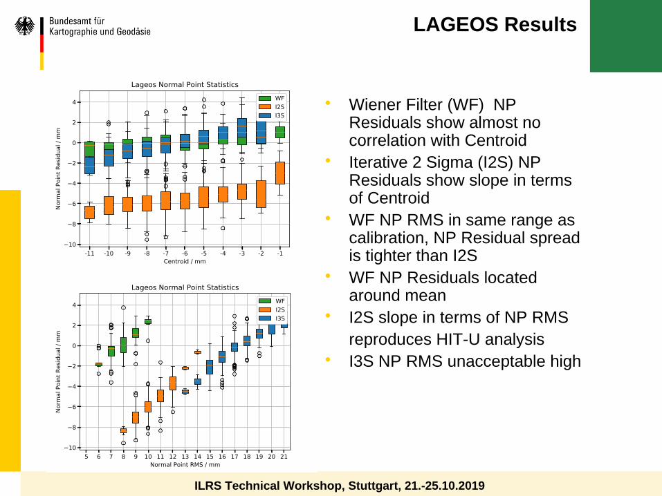
LAGEOS Results

-11 -10 -9 -8 -7 -6 -5 -4 -3 -2 -1Centroid / mm

10

8

6

4

2

0

2

4

Norm

al P

oint

Res

idua

l / m

m

Lageos Normal Point StatisticsWFI2SI3S

5 6 7 8 9 10 11 12 13 14 15 16 17 18 19 20 21Normal Point RMS / mm

10

8

6

4

2

0

2

4

Norm

al P

oint

Res

idua

l / m

m

Lageos Normal Point StatisticsWFI2SI3S

Wiener Filter (WF) NP Residuals show almost no correlation with Centroid

Iterative 2 Sigma (I2S) NP Residuals show slope in terms of Centroid

WF NP RMS in same range as calibration, NP Residual spread is tighter than I2S

WF NP Residuals located around mean

I2S slope in terms of NP RMS reproduces HIT-U analysis

I3S NP RMS unacceptable high


Etalon Results

5 6 7 8 9 1011121314151617181920212223242526272829Centroid / mm

40

30

20

10

0

10

20

Norm

al P

oint

Res

idua

l / m

m

Etalon Normal Point StatisticsWFI2SI3S

I2S,I3S NP Residuals show vast dependence on centroid, WF NP Residual variation with Centroid is subcentimeter

I3S NP RMS unacceptable high WF NP RMS in same range as

calibration, NP Residual spread is much tighter than I2S



Ajisai Results

WF NP Residual variation with Centroid is subcentimeter

I3S NP RMS unacceptable high I2S NP Residual vs. NP RMS

slope deviates by factor 2 from HIT-U Analysis

WF NP RMS in same range as calibration, NP Residual spread is much tighter than I2S



Lares Results

-20-19-18-17-16-15-14-13-12-11-10 -9 -8 -7 -6 -5 -4 -3 -2 -1 0 1 2Centroid / mm

6

4

2

0

2

4

6

8No

rmal

Poi

nt R

esid

ual /

mm

Lares Normal Point StatisticsWFI2SI3S

3 4 5 6 7 8 9 10 11 12 13 14 15 16 17 18 19 20Normal Point RMS / mm

6

4

2

0

2

4

6

8

10

Norm

al P

oint

Res

idua

l / m

m

Lares Normal Point StatisticsWFI2SI3S

WF NP Residual show the least variation with Centroid (-2 to +1mm)

I3S NP RMS unacceptable high I2S NP Residuals vs. NP RMS show

same slope as HIT-U Analysis WF NP RMS in same range as

calibration, NP Residual spread is much smaller than I2S



Starlette/Stella Results

-13 -12 -11 -10 -9 -8 -7 -6 -5 -4 -3 -2 -1Centroid / mm

2

0

2

4

6

Norm

al P

oint

Res

idua

l / m

mStarlette Normal Point Statistics

WFI2SI3S

5 6 7 8 9 10 11 12 13 14 15 16 17Normal Point RMS / mm

2

0

2

4

6

Norm

al P

oint

Res

idua

l / m

m

Starlette Normal Point StatisticsWFI2SI3S

WF NP Residual show the least variation with Centroid (+2 to +3mm)

I3S NP RMS unacceptable high I2S NP Residual vs. NP RMS

shows similar slope and signature as HIT-U Analysis

WF NP RMS in same range as calibration, NP Residual spread is much tighter than I2S

WF NP Residuals located around mean+2mm due to high bandwidth of Starlette response

Special Tuning of WF causes results to converge against I2S results


Conclusion

Iterative 3 sigma (I3S) editing is not an option due to high RMS values – it underestimates data quality

NP-Residual systematics in HIT-U Analysis can be explained to a large extent by the convergence properties of iterative 2 sigma editing

Wiener Filter NP-Algorithm is able to mitigate these systematics Wiener Filter NPs located around mean of Transfer Function for all

Satellites under consideration except Starlette(+2mm). With special tuning WF results converge against I2S results

Wiener Filter NPs show the least correlation with Centroid Wiener Filter NPs RMS in the same range as calibration, since

satellite signature is removed For large diameter Satellites Wiener Filter NPs are of superior quality

compared to iterative 2 sigma editing Wiener Filter NP procedure is consistent for LAGEOS, Etalon, Ajisai

and LARES

A review of where we stand in evaluating the quality of our NP's

Matthew WilkinsonNERC Space Geodesy Facility

2

◗The method to define normal points is fixed by the ILRS as the mean residual applied to a range at a central epoch within a fixed time window.

◗Stations are responsible for forming their own normal points. Some flatten their laser range measurements by adjusting an orbit prediction. Others do so by fitting a high order polynomial. Clipping of the range residuals is also set by the station.

◗The methods used to form normal points by the station must be described in the ILRS Site Log so that a centre-of-mass correction can be calculated.

Introduction

3

For a number of SLR stations, a variation was shown in the orbit fit range residuals of normal points that depends on the RMS.

This is due to the shape of the returning pulse and an inconsistency in the clipping applied on a pass by pass basis.

Otsubo, Systematic Range Error, IWLR, Annapolis 2014. https://cddis.nasa.gov/lw19/Program/index.html

Range vs RMS

4

This was also seen directly in the range data by plotting the distribution leading-edge-half-maximum (LEHM) and the NP mean difference against RMS.

Wilkinson, Systematics at the SGF, Herstmonceux, IWLR Potsdam, 2016.https://cddis.nasa.gov/lw20/docs/2016/papers/41-Wilkinson_paper.pdf

And this trend was shown to be partly caused by the variable orientation of LAGEOS from simulations of the satellite response.

Rodríguez, Variability of LAGEOS normal point sampling: causes and mitigation. Riga ILRS Technical Workshop, 2017.https://cddis.nasa.gov/2017_Technical_Workshop/docs/presentations/session2/ilrsTW2017_s2_Rodriguez.pdf

Range vs RMS

5

At Herstmonceux, currently the clipping is applied at ± 3σ from the centre of a Gaussian fit.

The σ value depends on the level of signal to noise and the satellite response profile.

Because the profile is not Gaussian, if tighter clipping is applied, due to a lower σ,then the normal point range will be shorter than if looser clipping were applied.

Forming Normal Points

6

To apply consistent clipping a stable point on the distribution is required, such as the leading-edge-half maximum (LEHM).

From the LEHM, fixed clipping can be applied that is set for all passes.

But, what level of clipping is best?

Clipping for Normal Points

7

NP mean – LEHM distributions from the clipped datasets are tighter.

Clearly, as the clipping applied is tighter the distance from the NP mean and the LEHM is reduced and the measurement is made closer to the front of the satellite.

Clipping Results

8

The clipping does not have much effect on the average pass range bias or the RMS of pass range bias.

An alternative way to look for any improvement is to account for modelling error in the solutions using a polynomial fit to each pass.

Analysis Results

9

A quadratic polynomial was removed from every pass to account for modelling errors.

The RMS of the remaining residuals was then calculated for each dataset for LAGEOS 1 and 2.

Using this method, it can be seen that the clipping reduces the normal point to normal point variation.

Analysis Results

It can process full-rate data or raw epoch-range data.

It could be used to process normal points from full-rate data to make assessments of the quality of our NPs.

The orbit adjustment PYTHON program from the SGF was released to the SLR community at the start of 2019. This was provided for stations to make comparisons with their methods to produce flattened range residuals and normal points.

OrbitNP.py

◗The normal point range residual dependency on single shot RMS can be minimised with controlled clipping about a well defined point on the satellite distribution.

◗Alternatively, allowing stations to calculate normal points using other methods could avoid this bias.

◗We did not find any evidence of this having an impact on the analysis products.

◗However, tighter clipping does improve the quality of the SLR measurements from Herstmonceux by decreasing the normal point variability.

◗Alternative methods to calculate normal points could be compared if the corresponding centre-of-mass values were defined.

Conclusions

1March 2020

NASA SLR Issues impacting Data Quality

Author: Van S HussonPeraton/NASA SLR Network

ILRS Central [email protected]

2March 2020

Agenda

u NASA SLR Site Survey Related Issuesu Three Potential NASA SLR Calibration Issues

3March 2020

NASA SLR Site Survey Related Issuesu NASA SLR survey accuracies:

Ø The accuracy in determining the NASA SLR system eccentricities in each component (North, East and Up) is at the 1-2 mm level, because direct measurements are not possible

Ø The accuracy is determining NASA SLR calibration distances is at the 2-4 mm level, because it depends in part upon the accuracy of the system eccentricities

Ø There is a potential 2 mm up discrepancy in the MOBLAS eccentricities based on IGN independent measurements of the self centering plate (ref: 2007 Tahiti survey)

Ø Axes of rotation are offset at the 1-2 mm level. Note: VLBI antennas may have the same issueu NASA SLR resource constraints have led to:

Ø Reduction in frequency of NASA SLR site surveysØ The contracting of surveying services to outside agencies who don’t necessarily fully

understand our SLR needsu Survey Management:

Ø The ILRS system eccentricity files and station site log do not always reflect the eccentricity data contained in the survey reports and vice versa

4March 2020

NASA SLR Satellite Interleaving Calibration Philosophy

u Pre satellite interleaving, each satellite (LEO, LAGEOS and HEO) were calibrated separately with a pre and post calibration taken immediately before and after the pass. Maximum time between a pre and post calibration was 50 to 55 minutes.

u Post satellite interleaving, one pre and post calibration are taken after a session of satellite tracking. The combined calibration is applied to all satellites (i.e. LEO, LAGEOS and HEO) in the session. Pre and Post calibrations are within 2 hours of each other. (See pass interleaving example on the right, 6 satellites with a common calibration. A timer series or receive energies.)

5

Differences between Calibration and Satellite

Station MarkerCalibration

FirerateCalibration

PMT (v)LAGEOS Firerate

LAGEOS PMT (v)

LARES Firerate

LARES PMT (v)

Etalon Firerate

Etalon PMT (v)

MOBLAS 4 7110 10 Hz 3200 5 to 10 Hz 3300 10 Hz 3200-3300 4 Hz 3200-3300MOBLAS 5 7090 10 Hz 3000 5 Hz 3100-3400 10 Hz 3300-3400 4 to 5 Hz 3300-3400MOBLAS 6 7501 10 Hz 2700 5 Hz 2800-3000 10 Hz 2700-3000 4 Hz 2900-3000MOBLAS 7 7105 10 Hz 2700 5 to 10 Hz 2900-3100 10 Hz 2800-3300 5 Hz 3300-3400MOBLAS 8 7124 10 Hz 3100 5 Hz 3100 10 Hz 3100 4 Hz 3100-3400TLRS 3 7403 5 Hz 3000 5 Hz 3000-3200 5 Hz 3000 N/A N/ATLRS 4 7119 5 Hz 2800 5 Hz 2900-3000 5 Hz 2800-3000 N/A N/A

Are these differences of the laser fire rates and PMT voltages between calibration and satellites inducinga range bias? If yes, 1. What is the magnitude of these biases?2. Are they recoverable?3. When did these changes take place since in the pre satellite interleaving, these differences did not exist?

6March 2020

Potential Calibration Issue #1 (Laser Fire Rate)

u Our laser maximum repetition rate is 10 Hz, but there were other constraints which kept the NASA SLR network at 5 HzØ Prior to the 2009 MOBLAS laser ranging controller (LRC) upgrade which enabled the laser to

fire at 10 Hz, all ranging was done at 5 HzØ Post LRC upgrade, calibrations and LEO tracking was performed at 10 Hz, but LAGEOS and HEO

were still constrained to 5 and 4 Hz; respectively, due to HP5370 TIU constraintsØ The laser can only be optimized at one rate and 5 Hz was chosen to maximize LAGEOS and HEO

data yieldØ The last few years, Event Timers have replaced the HP5370s, enabling 10 Hz and 5 Hz ranging

on LAGEOS and HEOs; respectively; some of the time dependent upon the satellite range

u Question #1: Since the characteristics (e.g. beam divergence) of the laser change when the fire rate is altered, does that impact system delay and how much if it does?

7

7105 MOBLAS-7 LAGEOS-1 Pass on Oct 25, 2019

These graphs are a time series of receive energies of a high elevation 7105 LAGEOS pass (i.e. > 80 degrees) where the laser fire rate was toggled between 5 and 10 Hz. The receive energies decrease as the mount has trouble keeping up as the pass approaches the satellite Point of Closest Approach (PCA). The ranges and elevations are plotted on the right

axes on the left and right charts; respectively.

8

Summary of 5 pps vs 10 pps Ground Tests

System System Delay Diffs (10 pps – 5 pps) in mm

10 pps LRC Upgrade

MOBLAS 4 2.3 22-Sep-2009

MOBLAS 5 1.5 28-Sep-2009

MOBLAS 6 TBD 04-Sep-2009

MOBLAS 7 TBD 11-Jul-2009

MOBLAS 8 -1.0 03-Nov-2009

9

7105 MOBLAS-7 LAGEOS-1 Pass on Oct 25, 2019

This is the same time series of receive energies from the same 7105 LAGEOS pass including the pre and post calibrations. On the right axes are

the PMT voltages.

The satellite PMT voltage is in the C2 CRD record. When the NASA SLR software was written to

create CRDs, the PMT voltages weren’t varied from one satellite to another, so the PMT voltage was placed in static config file. Also, the current

CRD V2 format does not have a field for calibration PMT voltage in the 40 or 41

calibration records.

10

Potential Calibration Issue #2 (altering PMT voltages)

u Starting in 2011, NASA SLR stations were permitted to use higher voltages on satellites with weaker signals (i.e. LARES, LAGEOS, Etalon) to maximize data yield.

u Does changing the PMT voltage change the system delay and if so how much?

11

MOBLAS 7 PMT Voltage Test

The scatter increases as the PMT voltage increases. Currently MOBLAS 7 calibrates at

2700 volts; LARES data is taken between 2800 to 3300 volts; LAGEOS data is taken between 2900 to 3100 volts; and Etalon

data is taken between 3300 to 3400 volts.

We plan to have the other NASA SLR systems perform this test so we can

characterize the impact. We also need to determine if these results are repeatable.

12

Potential Calibration Issue #3 (Receive Energy)u Pre satellite interleaving, the

stations would calibrate each pass individually, station operators where trained to try and mimic the dynamic range of the satellite receive energies during calibration.

u On this same LAGEOS pass residuals were added to the right axes and there is a several mm shift in the residuals as the receive energy decreases.

u How much does system delay depend upon receive energy and how well do our systems calibrate?

13

7110 MOBLAS-4 LAGEOS-2 Analysis

This is an aggregation of 7110 residuals from 6 days in Aug 2019. The calibration

and LAGEOS-2 residuals are binned vs receive energy. Both LAGEOS-2 and

calibration show similar trends at the weaker signal levels. Unfortunately, the

area between the cumulative distributions is quite large and thus there is a potential

for a range bias.

14

Conclusions and Next Steps

u ConclusionsØ Surveying techniques are a limiting factor in absolute data accuracy.ØMillimeter levels biases are being introduced in our current calibration scheme.

u Next StepsØ Investigate the feasibility of having close-in calibration targets.ØWe need to characterize these potential errors sources for each of our systems and

determine if the results are repeatable. Then document the finding and if deemed necessary update the data handling files.

ØThe ILRS has recommended we reduce systematic biases caused by each component to the sub-mm level [Prochazka 2015]. However, not ever mission needs mm level accuracy. We recommend the ILRS determine the accuracy requirements for each mission and then we need to re-evaluate our calibration procedures to balance maximizing data accuracy on the high value satellites without sacrificing data quantity.

15March 2020

Backup Material

16March 2020

NASA SLR Survey Summary (last two)

Location Marker System Last Survey OrganizationSLR System

Reference Point

SLR Calibration

PiersMonument Peak,

USA7110 MOBLAS 4 May-2018 NGS Yes Yes

Nov-2011 NASA Yes YesYarragadee,

Australia7090 MOBLAS 5 Mar-2014 Geoscience Australia Yes ?

Jul-2010 Geoscience Australia Yes ?Hartebeesthoek,

South Africa7501 MOBLAS 6 Feb-2014 IGN Yes Yes

Aug-2003 IGN Yes YesGreenbelt, USA 7105 MOBLAS 7 Aug-2012 NGS Yes Yes

Mar-2008 NASA Yes YesTahiti, French

Polynesia7124 MOBLAS 8 Oct-2007 IGN Yes No

Jan-2002 NASA Yes YesArequipa, Peru 7403 TLRS-3 Jan-2013 IGN No Yes

May-2007 NASA Yes YesHaleakala, USA 7119 TLRS-4 Mar-2019 NGS No Yes

May-2013 NASA Yes Yes

To support 1 mm accuracy recommendations, surveys need to be more frequent.

17March 2020

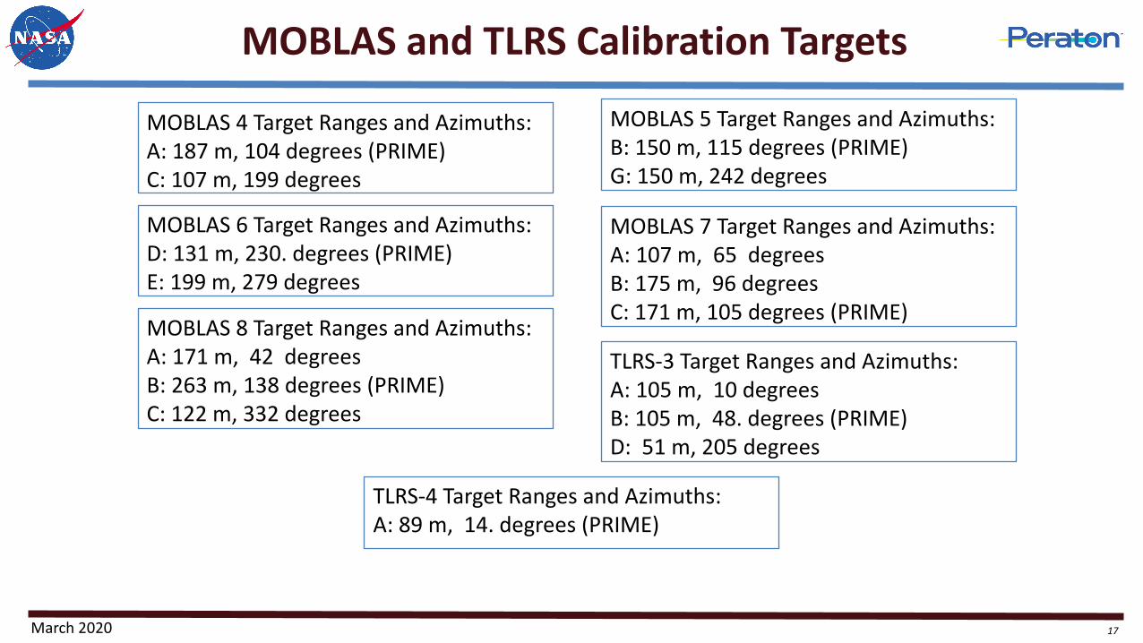
MOBLAS and TLRS Calibration Targets

MOBLAS 7 Target Ranges and Azimuths:A: 107 m, 65 degreesB: 175 m, 96 degreesC: 171 m, 105 degrees (PRIME)

MOBLAS 4 Target Ranges and Azimuths:A: 187 m, 104 degrees (PRIME)C: 107 m, 199 degrees

MOBLAS 5 Target Ranges and Azimuths:B: 150 m, 115 degrees (PRIME)G: 150 m, 242 degrees

MOBLAS 6 Target Ranges and Azimuths:D: 131 m, 230. degrees (PRIME)E: 199 m, 279 degrees

MOBLAS 8 Target Ranges and Azimuths:A: 171 m, 42 degreesB: 263 m, 138 degrees (PRIME)C: 122 m, 332 degrees

TLRS-3 Target Ranges and Azimuths:A: 105 m, 10 degrees B: 105 m, 48. degrees (PRIME)D: 51 m, 205 degrees

TLRS-4 Target Ranges and Azimuths:A: 89 m, 14. degrees (PRIME)

18March 2020

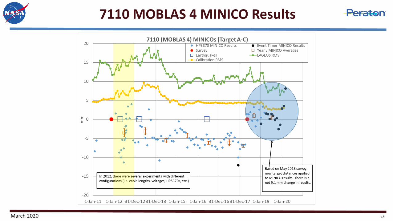
7110 MOBLAS 4 MINICO Results

19March 2020

MOBLAS 4 and 7 MINICO Results

Post ETM, MOBLAS 7 results are more stable than MOBLAS 4

20

MOBLAS-4 Laser Fire Rate Ground Test (5 vs 10 pps)

MOBLAS 4 did a laser fire test from both of their two targets A&C (Target A is prime). Since we are looking for millimetersthe results on C are more accurate since the mean and dynamic range of receive energies were better maintained.

21

7090 MOBLAS-5 Diurnal Range Bias Analysis

Toshi’s yearly aggregate analysis starting in 2015 has shown mm level diurnal effects in some of the NASA systemsAre these effects real? If so, are PMT voltage changes and/or receive energies differences the root cause?

improved ilrs modeling: vlbi-slr scale difference 0.23 ppb

Documents