import demand elasticities revisited - wiiw...import demand elasticities revisited mahdi ghodsi...

NOVEMBER 2016

Working Paper 132

Import Demand Elasticities Revisited Mahdi Ghodsi, Julia Grübler, Robert Stehrer

The Vienna Institute for International Economic Studies Wiener Institut für Internationale Wirtschaftsvergleiche

Import Demand Elasticities Revisited MAHDI GHODSI JULIA GRÜBLER ROBERT STEHRER

Mahdi Ghodsi and Julia Grübler are Research Economists at the Vienna Institute for International Economic Studies (wiiw). Robert Stehrer is Scientific Director of wiiw. This paper was produced as part of the PRONTO (Productivity, Non-Tariff Measures and Openness) project funded by the European Commission under the 7th Framework Programme, grant agreement no: 613504.

Abstract

In this paper, we present import demand elasticities estimated for 167 countries over

5,124 products at the six-digit level of the Harmonised System. Following the semiflexible translog

GDP function approach proposed by Kee et al. (2008), we estimate unilateral import demand

elasticities for the period 1996-2014. Results are differentiated by country and product

characteristics. South Asia and North America are associated with the most elastic import demand.

Countries exhibiting the highest average elasticities belong to the economically most important

countries in their respective regions, while countries with the lowest import demand elasticities are

typically small island states. Import-weighted results suggest that especially countries rich in

natural resources – particularly fossil fuels – are facing an inelastic import demand, with the agri-

food sector for these states being more price-responsive than the manufacturing sector. Demand is

found to be least price-sensitive for machinery and electrical equipment, and most price-elastic for

the energy sectors. Distinguishing between the use of products, the highest import demand

elasticities are associated with intermediate goods, which appears particularly noteworthy in the

context of an increasing importance of global value chains, the global trade slowdown since 2011

and ongoing negotiations of mega-regional trade deals.

Keywords: international trade, import demand, elasticity

JEL classification: D12, F14

CONTENTS

1. Introduction ...................................................................................................................................................... 1

2. The theoretical framework ....................................................................................................................... 2

3. Methodology and data ................................................................................................................................ 4

4. Empirical results ............................................................................................................................................. 7

5. Robustness ...................................................................................................................................................... 22

6. Conclusion ...................................................................................................................................................... 25

7. References ....................................................................................................................................................... 26

Appendix ...................................................................................................................................................................... 28

TABLES AND FIGURES

Table 1 / Elasticities by importer .............................................................................................................. 10

Table 2 / Regional elasticities .................................................................................................................. 14

Table 3 / Regression of binding import demand elasticities on country characteristics ........................... 16

Table 4 / Elasticities by WIOD sector ....................................................................................................... 19

Table 5 / Elasticities by product use ......................................................................................................... 20

Table 6 / Regression of binding import demand elasticities on product characteristics ........................... 21

Figure 1 / Distribution of elasticity estimates: FE, FEIV, SSB .................................................................... 7

Figure 2 / Distribution of elasticity estimates at the HS 6-digit level ........................................................... 8

Figure 3 / Simple average binding elasticities per country ......................................................................... 9

Figure 4 / Binding elasticities over income ............................................................................................... 15

Figure 5 / Binding simple average elasticities per HS Section ................................................................. 18

Figure 6 / Binding elasticities over income: estimates per income group ................................................ 23

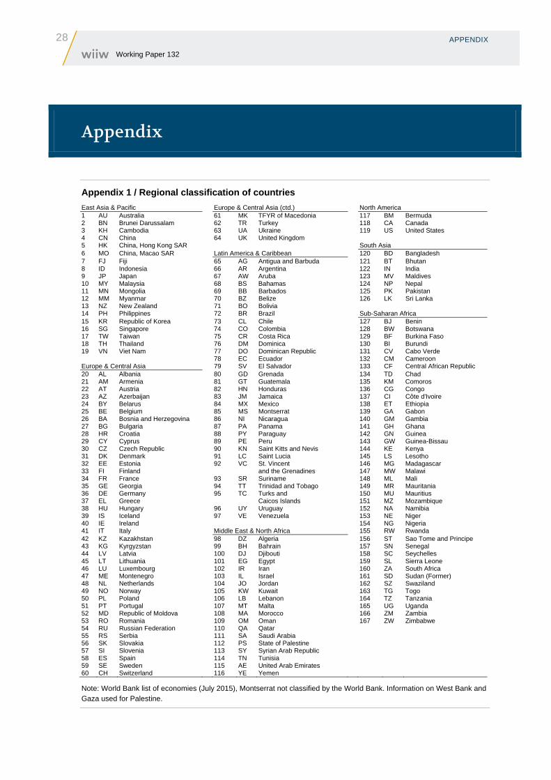
Appendix 1 / Regional classification of countries ..................................................................................... 28

Appendix 2 / Income classification of countries ....................................................................................... 29

INTRODUCTION

1 Working Paper 132

1. Introduction

The set of applied trade policy instruments is constantly increasing. In addition to traditional trade policy

tools such as tariffs or quotas, non-tariff measures such as sanitary and phytosanitary measures,

technical barriers to trade or antidumping practices feature prominently in ongoing trade negotiations.

The number of trade agreements as well as their geographical scope and depth of their agendas is

surging. Mega-regional trade agreements such as the Transatlantic Trade and Investment Partnership

(TTIP) between the EU and the United States, the Transpacific Partnership (TPP) centred around the

US, and the Regional Comprehensive Economic Partnership (RCEP) including China bear the potential

of exerting a substantial impact on quantities and prices of imported products.

In order to compare the impact of different trade policies it is often necessary to make use of import

demand elasticities (e.g. Kee et al., 2009; Nizovtsev and Skiba, 2016) answering the question: What

would be the percentage change in import quantities if the price of the imported good increased by 1%?

Trade policy is frequently operational at the tariff line level. However, there are only few studies which

allow the evaluation of demand elasticities for a broad set of products at the very disaggregated product

level (e.g. Kee et al., 2008; Feenstra and Romalis, 2014). Available studies have a strong focus on

either selected products (e.g. Panagariya et al., 2001; Altinay, 2007) and/or particular importers

(e.g. Broda and Weinstein, 2006; Soderbery, 2015).

To the best of our knowledge, the investigation by Kee et al. (2008) is the only work that evaluated price

elasticities of import demand for a wide range of products and countries, having the inherent additional

advantage of rendering elasticities across countries and products more comparable through the

application of a single methodology and dataset for all.

Overall, Kee et al. (2008) estimated more than 300,000 import demand elasticities across 117 countries

for about 4,900 products at the 6-digit level of the Harmonised System (HS revision 1988) for the period

1988-2001. Their estimates are frequently used in various policy analysis (e.g. Kee et al., 2009; Maoz,

2009; Bratt, 2014; Peterson and Thies, 2014; Beghin et al., 2015).

This paper constitutes an update of their work by computing importer-specific import demand elasticities

for the more recent period 1996-2014 (HS revision 1996) and presents differences across countries,

regions and income levels, as well as by products and sectors. Improved data availability and the

inclusion of products not considered in HS revision 1988 allows us to estimate about twice as many

import demand elasticities for 167 importing countries and 5124 products.

The remainder of this paper is structured as follows. Section 2 explains the theoretical framework.

Section 3 describes the data used and the empirical strategy. Section 4 presents the empirical results

and Section 5 discusses the robustness of the findings. The final section concludes.

2 THE THEORETICAL FRAMEWORK Working Paper 132

2. The theoretical framework

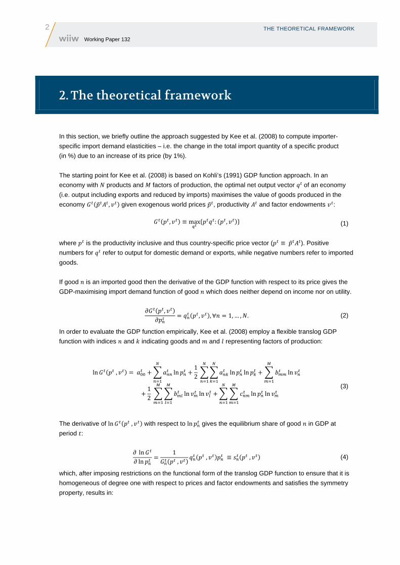
In this section, we briefly outline the approach suggested by Kee et al. (2008) to compute importer-

specific import demand elasticities – i.e. the change in the total import quantity of a specific product

(in %) due to an increase of its price (by 1%).

The starting point for Kee et al. (2008) is based on Kohli’s (1991) GDP function approach. In an

economy with products and factors of production, the optimal net output vector of an economy

(i.e. output including exports and reduced by imports) maximises the value of goods produced in the

economy , given exogenous world prices , productivity and factor endowments :

, ≡ max : , (1)

where is the productivity inclusive and thus country-specific price vector ( ≡ ). Positive

numbers for refer to output for domestic demand or exports, while negative numbers refer to imported

goods.

If good is an imported good then the derivative of the GDP function with respect to its price gives the

GDP-maximising import demand function of good which does neither depend on income nor on utility.

,, , ∀ 1, … , . (2)

In order to evaluate the GDP function empirically, Kee et al. (2008) employ a flexible translog GDP

function with indices and indicating goods and and representing factors of production:

ln , ln12 ln ln ln

12 ln ln ln ln

(3)

The derivative of ln , with respect to ln gives the equilibrium share of good in GDP at

period :

∂lnln

1,

, ≡ , (4)

which, after imposing restrictions on the functional form of the translog GDP function to ensure that it is

homogeneous of degree one with respect to prices and factor endowments and satisfies the symmetry

property, results in:

THE THEORETICAL FRAMEWORK

3 Working Paper 132

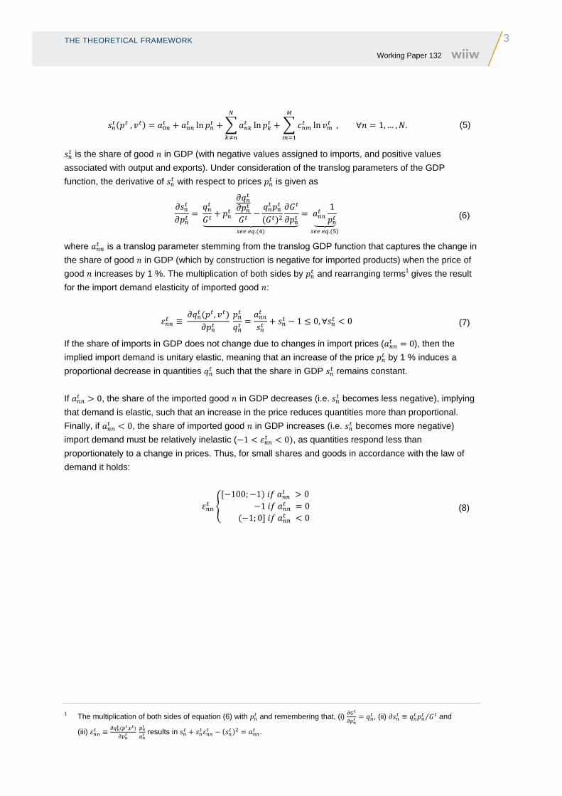
, ln ln ln , ∀ 1, … , . (5)

is the share of good in GDP (with negative values assigned to imports, and positive values

associated with output and exports). Under consideration of the translog parameters of the GDP

function, the derivative of with respect to prices is given as

.

1

.

(6)

where is a translog parameter stemming from the translog GDP function that captures the change in

the share of good in GDP (which by construction is negative for imported products) when the price of

good increases by 1 %. The multiplication of both sides by and rearranging terms1 gives the result

for the import demand elasticity of imported good :

≡,

1 0, ∀ 0 (7)

If the share of imports in GDP does not change due to changes in import prices ( 0), then the

implied import demand is unitary elastic, meaning that an increase of the price by 1 % induces a

proportional decrease in quantities such that the share in GDP remains constant.

If 0, the share of the imported good in GDP decreases (i.e. becomes less negative), implying

that demand is elastic, such that an increase in the price reduces quantities more than proportional.

Finally, if 0, the share of imported good in GDP increases (i.e. becomes more negative)

import demand must be relatively inelastic ( 1 0 , as quantities respond less than

proportionately to a change in prices. Thus, for small shares and goods in accordance with the law of

demand it holds:

100; 1 0 1 0 1; 0 0

(8)

1 The multiplication of both sides of equation (6) with and remembering that, (i) , (ii) ≡ ⁄ and

(iii) ≡, results in .

4 METHODOLOGY AND DATA Working Paper 132

3. Methodology and data

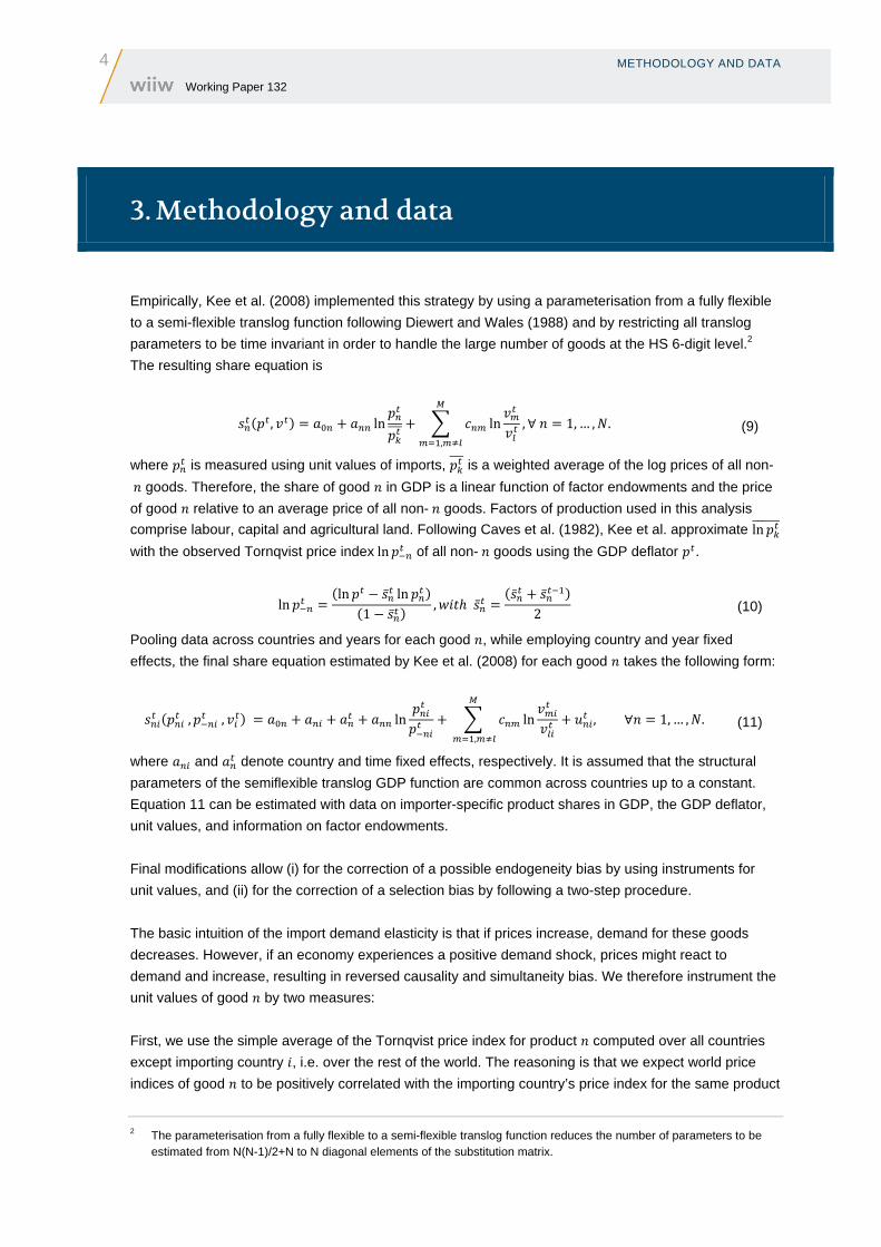
Empirically, Kee et al. (2008) implemented this strategy by using a parameterisation from a fully flexible

to a semi-flexible translog function following Diewert and Wales (1988) and by restricting all translog

parameters to be time invariant in order to handle the large number of goods at the HS 6-digit level.2

The resulting share equation is

, ln ln,

, ∀ 1, … , . (9)

where is measured using unit values of imports, is a weighted average of the log prices of all non-

goods. Therefore, the share of good in GDP is a linear function of factor endowments and the price

of good relative to an average price of all non- goods. Factors of production used in this analysis

comprise labour, capital and agricultural land. Following Caves et al. (1982), Kee et al. approximate ln

with the observed Tornqvist price indexln of all non- goods using the GDP deflator .

lnln ln

1 ,

2

(10)

Pooling data across countries and years for each good , while employing country and year fixed

effects, the final share equation estimated by Kee et al. (2008) for each good takes the following form:

, , ln ln,

, ∀ 1, … , . (11)

where and denote country and time fixed effects, respectively. It is assumed that the structural

parameters of the semiflexible translog GDP function are common across countries up to a constant.

Equation 11 can be estimated with data on importer-specific product shares in GDP, the GDP deflator,

unit values, and information on factor endowments.

Final modifications allow (i) for the correction of a possible endogeneity bias by using instruments for

unit values, and (ii) for the correction of a selection bias by following a two-step procedure.

The basic intuition of the import demand elasticity is that if prices increase, demand for these goods

decreases. However, if an economy experiences a positive demand shock, prices might react to

demand and increase, resulting in reversed causality and simultaneity bias. We therefore instrument the

unit values of good by two measures:

First, we use the simple average of the Tornqvist price index for product computed over all countries

except importing country , i.e. over the rest of the world. The reasoning is that we expect world price

indices of good to be positively correlated with the importing country’s price index for the same product

2 The parameterisation from a fully flexible to a semi-flexible translog function reduces the number of parameters to be estimated from N(N-1)/2+N to N diagonal elements of the substitution matrix.

METHODOLOGY AND DATA

5 Working Paper 132

thereby affecting import demand. However, while a domestic demand shock might impact an economy’s

domestic and import prices, we do not expect that domestic demand for imported products is shaping

price indices of the rest of the world.

Remembering from equation (10) that the price of non- goods can be expressed as the GDP deflator

adjusted for the share and price of good , the price index for good over all non- importing countries

(indexed ) can be computed in a similar fashion:

ln

ln ∑ ∑ln ∑

1 ∑

, (12)

A second instrument is the trade-weighted average distance of the importing country to its trading

partners. The intuition being that the price of imported products is expected to be higher for products that

have to be transported over greater distances, while distance might not be correlated with domestic

demand for good .

(13)

where is the physical distance between importer and exporter and is the share of an

exporter in total exports of good in period .

Results using these instruments might, however, still suffer from a selection bias, as unit values entering

our analysis are calculated based on positive import flows. Country and year fixed effects can reduce the

bias resulting from unobserved variables. Yet, due to the possibility that zero trade flows in our data are

the result of countries’ selection not to import, we follow an amended form of the Heckman two-stage

estimation procedure. In the first step of the two-stage estimation procedure, the selection equation

(14a) evaluates the probability of non-zero trade flows. The dependent variable is equal to 1 if the share

of good in country ’s GDP is smaller than zero (i.e. imports are greater than zero). It is regressed on a

product-specific term , time fixed effects , country fixed effects , as well as the previously

introduced instruments and factor endowments, captured in . is an error term.

From this first step, the inverse Mills ratio ) is obtained, which enters the outcome equation (15) in

the second step as an explanatory variable, which should solve the omitted variable bias in the presence

of sample selection. A drawback of this procedure is, that probit model estimations with country fixed

effects suffer from the incidental parameters problem. It means that as we are using a big panel data set

incorporating many fixed effects, probit models are more likely to render biased and inconsistent

estimates, as they do not converge to their true value as the number of parameters (i.e. fixed effects)

increases with sample size. In line with Kee et al. (2008) we therefore substitute country fixed effects

with time averages of the exogenous variables and instruments in the first stage (equation 14b).

0 , ∀ 1, … , . (14a)

0 , ∀ 1, … , . (14b)

6 METHODOLOGY AND DATA Working Paper 132

| 0 ln ln ,

,

∀ 1, … , .

(15)

Finally, using the average import shares of each importing country and estimates of the resulting

import demand elasticity of country for good is computed as

≡ ,

1. (16)

The data necessary for estimation was compiled from different sources. Import values and quantities

were taken from the Commodity Trade Statistics Database (COMTRADE) for the period 1995-2014. It

covers 5,221 products at the HS 6-digit (rev. 1996) level. Data on agricultural land in square kilometres

was retrieved from the World Development Indicators (WDI) database of the World Bank and

complemented by data provided by the Food and Agriculture Organization of the United Nations (FAO).

Data on GDP, physical capital and labour was collected from the Penn World Tables 9.0 (Feenstra et al.,

2015).

EMPIRICAL RESULTS

7 Working Paper 132

4. Empirical results

On average, each HS 6-digit product in our sample was imported by 155 countries, with a minimum of

17 importers for petroleum oil obtained from bituminous minerals (HS 271094) and a maximum of

167 importers for 378 different products at the HS 6-digit level. Countries in the sample imported on

average 4,790 products, ranging from a minimum of 1,593 products for Djibouti to 5,121 products for

France. We dropped observations for which bilateral import values were reported but bilateral quantities

were missing in order to avoid a bias of unit values entering our estimation procedure.

Following the methodology presented in Section 3, we performed three estimations: first, employing

simple fixed effects (FE), second, introducing instrument variables to the fixed effects estimation

procedure (FEIV) and finally, substituting the fixed effects approach by a two-step procedure to account

for a possible sample selection bias (SSB).

Based on these results we constructed our final set of elasticity estimates. We based our decision when

to replace FE results by FEIV results upon two criteria: (i) The Hansen J-statistic reports the validity of

instruments, with the null hypothesis that instruments are exogenous. (ii) The Anderson-Rubin F-statistic

shows whether instruments have an impact on the endogenous variable, with the null hypothesis that

the endogenous regressors in the structural equation are jointly equal to zero. We therefore replaced FE

estimates by FEIV results only if the Hansen J-statistic was greater than 0.1 and the Anderson-Rubin

F-statistic was smaller than 0.1.

In addition to these two instrument variable criteria, when the coefficient of the inverse mills ratio ( ) in

equation (15), indicating whether our results might suffer from sample selection bias, was found to be

statistically significantly different form zero at the 10% level FEIV results were replaced by SSB results.

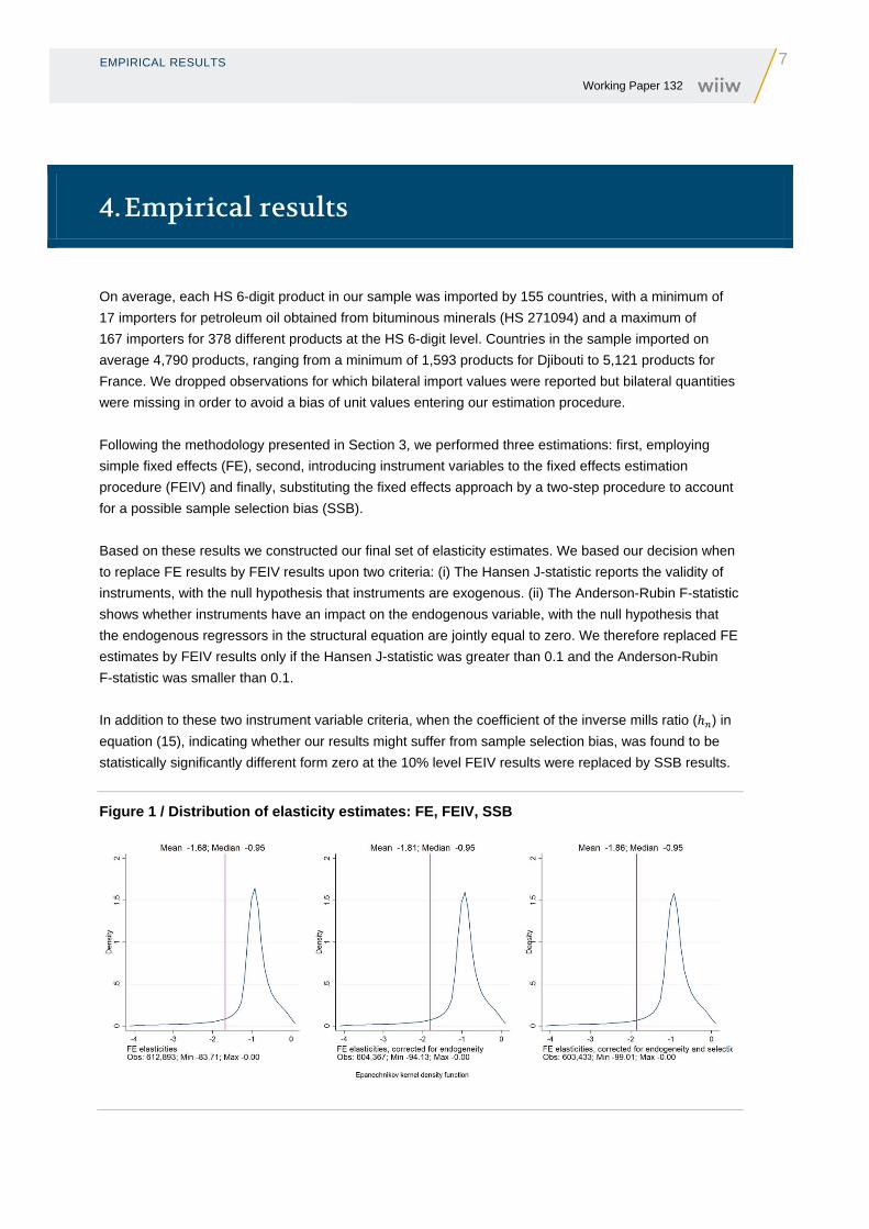
Figure 1 / Distribution of elasticity estimates: FE, FEIV, SSB

8 EMPIRICAL RESULTS Working Paper 132

Figure 1 shows the distribution of elasticities along our modifications. Throughout, it looks quite similar,

with mean elasticities smaller, i.e. more negative, than -1.6 but median elasticities larger than -1.

Corrections for endogeneity and a selection bias leave median values unchanged but shift mean values

towards -2.

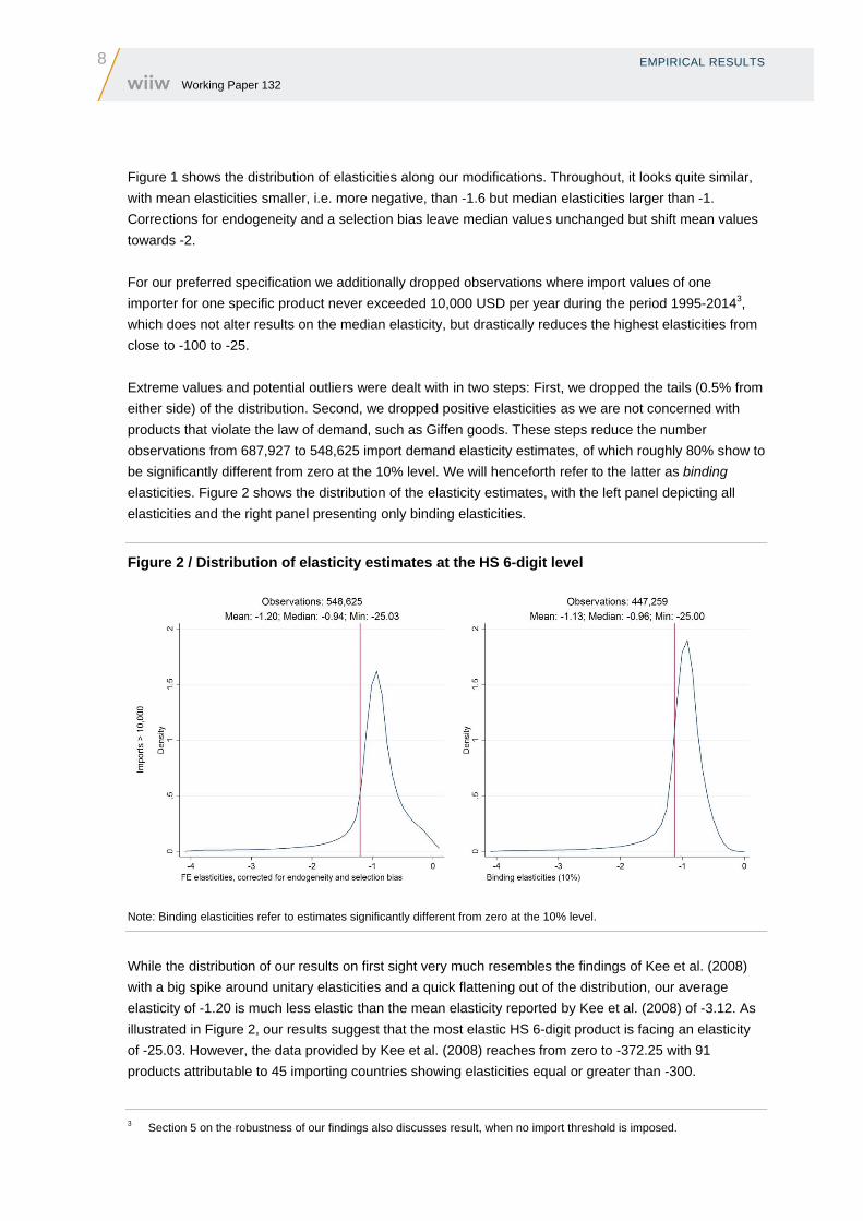
For our preferred specification we additionally dropped observations where import values of one

importer for one specific product never exceeded 10,000 USD per year during the period 1995-20143,

which does not alter results on the median elasticity, but drastically reduces the highest elasticities from

close to -100 to -25.

Extreme values and potential outliers were dealt with in two steps: First, we dropped the tails (0.5% from

either side) of the distribution. Second, we dropped positive elasticities as we are not concerned with

products that violate the law of demand, such as Giffen goods. These steps reduce the number

observations from 687,927 to 548,625 import demand elasticity estimates, of which roughly 80% show to

be significantly different from zero at the 10% level. We will henceforth refer to the latter as binding

elasticities. Figure 2 shows the distribution of the elasticity estimates, with the left panel depicting all

elasticities and the right panel presenting only binding elasticities.

Figure 2 / Distribution of elasticity estimates at the HS 6-digit level

Note: Binding elasticities refer to estimates significantly different from zero at the 10% level.

While the distribution of our results on first sight very much resembles the findings of Kee et al. (2008)

with a big spike around unitary elasticities and a quick flattening out of the distribution, our average

elasticity of -1.20 is much less elastic than the mean elasticity reported by Kee et al. (2008) of -3.12. As

illustrated in Figure 2, our results suggest that the most elastic HS 6-digit product is facing an elasticity

of -25.03. However, the data provided by Kee et al. (2008) reaches from zero to -372.25 with 91

products attributable to 45 importing countries showing elasticities equal or greater than -300.

3 Section 5 on the robustness of our findings also discusses result, when no import threshold is imposed.

EMPIRICAL RESULTS

9 Working Paper 132

4.1. ELASTICITIES BY IMPORTER

While Figure 1 and Figure 2 have shown the distribution of our estimated import demand elasticities over

all HS 6-digit products and importers, this section aims to discuss geographical patterns of this

distribution. We start by discussing elasticity aggregates by country and proceed by computing regional

average elasticities and finally illustrate average elasticities by income group.

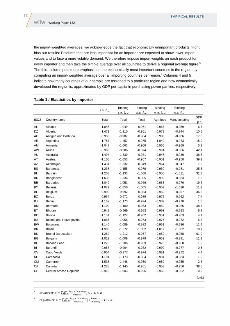
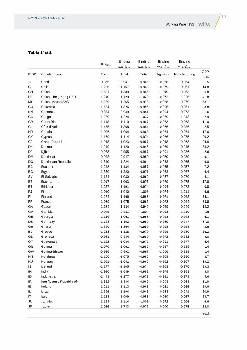
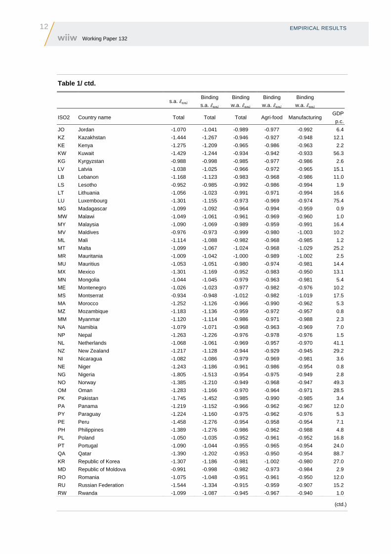
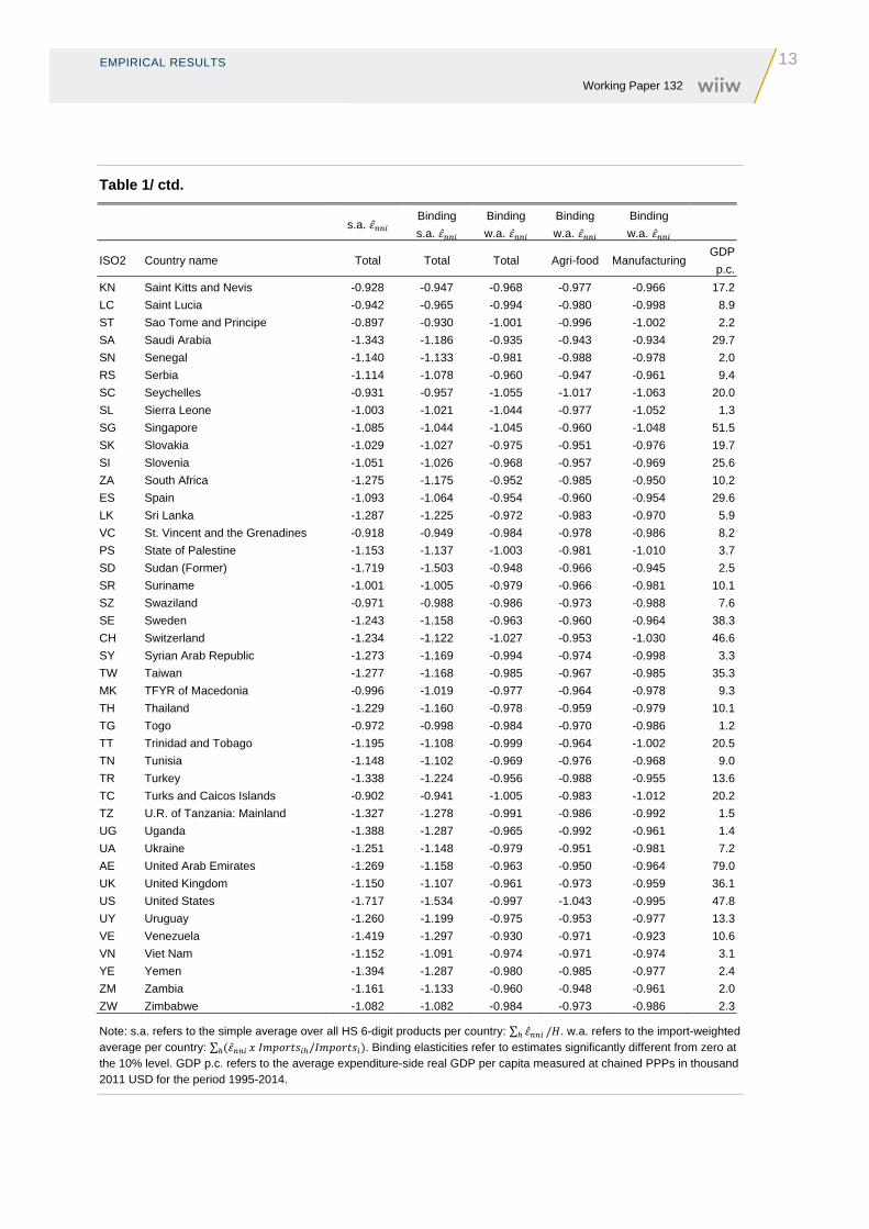
Table 1 summarises our results per country. The first two columns report our findings as simple average

(s.a.) elasticities. Results shown in the second and subsequent columns are restricted to products for

which elasticities were found to be binding, i.e. significantly different from zero at the 10% level. The

third column of Table 1 shows results of binding elasticities when import-weights are applied. Columns

four and five split up these import-weighted results into the agri-food and the manufacturing sector.

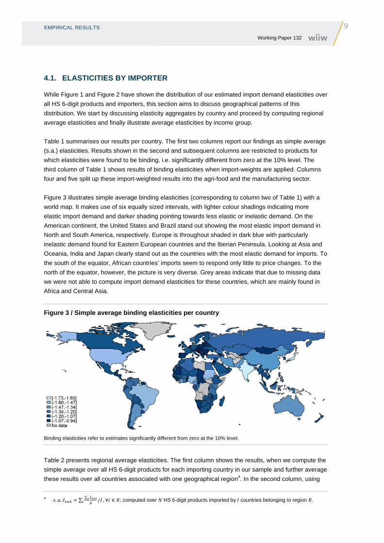
Figure 3 illustrates simple average binding elasticities (corresponding to column two of Table 1) with a

world map. It makes use of six equally sized intervals, with lighter colour shadings indicating more

elastic import demand and darker shading pointing towards less elastic or inelastic demand. On the

American continent, the United States and Brazil stand out showing the most elastic import demand in

North and South America, respectively. Europe is throughout shaded in dark blue with particularly

inelastic demand found for Eastern European countries and the Iberian Peninsula. Looking at Asia and

Oceania, India and Japan clearly stand out as the countries with the most elastic demand for imports. To

the south of the equator, African countries’ imports seem to respond only little to price changes. To the

north of the equator, however, the picture is very diverse. Grey areas indicate that due to missing data

we were not able to compute import demand elasticities for these countries, which are mainly found in

Africa and Central Asia.

Figure 3 / Simple average binding elasticities per country

Binding elasticities refer to estimates significantly different from zero at the 10% level.

Table 2 presents regional average elasticities. The first column shows the results, when we compute the

simple average over all HS 6-digit products for each importing country in our sample and further average

these results over all countries associated with one geographical region4. In the second column, using

4 . . ∑∑

/ , ∀ ∈ ; computed over HS 6-digit products imported by countries belonging to region .


the import-weighted averages, we acknowledge the fact that economically unimportant products might

bias our results: Products that are less important for an importer are expected to show lower import

values and to face a more volatile demand. We therefore impose import weights on each product for

every importer and then take the simple average over all countries to derive a regional average figure.5

The third column puts more emphasis on the economically most important countries in the region, by

computing an import-weighted average over all importing countries per region.6 Columns 4 and 5

indicate how many countries of our sample are assigned to a particular region and how economically

developed the region is, approximated by GDP per capita in purchasing power parities, respectively.

Table 1 / Elasticities by importer

s.a. Binding

s.a.

Binding

w.a.

Binding

w.a.

Binding

w.a.

ISO2 Country name Total Total Total Agri-food Manufacturing GDP

p.c.

AL Albania -1.045 -1.049 -0.961 -0.967 -0.959 6.7

DZ Algeria -1.472 -1.310 -0.951 -0.978 -0.944 10.5

AG Antigua and Barbuda -0.958 -0.987 -0.984 -0.980 -0.986 17.6

AR Argentina -1.757 -1.457 -0.975 -1.040 -0.973 15.9

AM Armenia -1.047 -1.063 -0.968 -0.966 -0.969 5.2

AW Aruba -0.969 -0.986 -0.974 -0.991 -0.966 42.1

AU Australia -1.494 -1.339 -0.931 -0.945 -0.930 38.6

AT Austria -1.106 -1.053 -0.957 -0.951 -0.958 39.1

AZ Azerbaijan -1.431 -1.332 -0.949 -0.964 -0.947 7.5

BS Bahamas -1.238 -1.155 -0.979 -0.969 -0.981 25.5

BH Bahrain -1.203 -1.133 -1.006 -0.956 -1.011 31.3

BD Bangladesh -1.635 -1.336 -0.985 -0.992 -0.983 1.8

BB Barbados -1.049 -1.051 -0.969 -0.963 -0.970 19.6

BY Belarus -1.079 -1.050 -1.005 -0.957 -1.010 11.9

BE Belgium -0.990 -0.992 -0.984 -0.959 -0.987 36.8

BZ Belize -0.964 -0.972 -0.989 -0.972 -0.992 7.4

BJ Benin -1.162 -1.173 -0.974 -0.982 -0.970 1.6

BM Bermuda -1.100 -1.100 -0.963 -0.950 -0.966 48.7

BT Bhutan -0.942 -0.969 -0.993 -0.993 -0.993 5.2

BO Bolivia -1.151 -1.127 -0.962 -0.951 -0.963 4.1

BA Bosnia and Herzegovina -1.086 -1.058 -0.973 -0.976 -0.972 6.8

BW Botswana -1.140 -1.089 -0.982 -0.951 -0.986 11.4

BR Brazil -1.903 -1.572 -1.002 -1.017 -1.002 10.7

BN Brunei Darussalam -1.262 -1.212 -0.957 -0.952 -0.958 61.0

BG Bulgaria -1.022 -1.009 -0.979 -0.952 -0.981 11.9

BF Burkina Faso -1.276 -1.206 -0.969 -0.970 -0.968 1.2

BI Burundi -0.967 -0.994 -0.982 -0.999 -0.977 0.6

CV Cabo Verde -0.954 -0.977 -0.974 -0.981 -0.972 4.4

KH Cambodia -1.194 -1.173 -0.984 -0.994 -0.983 1.9

CM Cameroon -1.536 -1.446 -0.960 -0.980 -0.955 2.3

CA Canada -1.228 -1.145 -0.951 -0.953 -0.950 38.6

CF Central African Republic -0.919 -1.003 -0.956 -0.968 -0.952 0.9

(ctd.)

5 . . ∑ ∑ / , ∀ ∈

6 . . ∑ ∑ / , ∀ ∈

EMPIRICAL RESULTS

11 Working Paper 132

Table 1/ ctd.

s.a. Binding

s.a.

Binding

w.a.

Binding

w.a.

Binding

w.a.


p.c.

TD Chad -0.865 -0.941 -0.965 -0.968 -0.964 1.5

CL Chile -1.286 -1.157 -0.963 -0.979 -0.961 14.8

CN China -1.621 -1.389 -0.966 -1.049 -0.963 6.8

HK China, Hong Kong SAR -1.240 -1.129 -1.023 -0.972 -1.025 41.8

MO China, Macao SAR -1.289 -1.265 -0.978 -0.968 -0.979 58.1

CO Colombia -1.524 -1.326 -0.956 -0.995 -0.951 8.8

KM Comoros -0.884 -0.949 -0.981 -0.994 -0.973 1.6

CG Congo -1.289 -1.224 -1.037 -0.969 -1.043 2.9

CR Costa Rica -1.148 -1.110 -0.967 -0.963 -0.968 11.0

CI Côte d'Ivoire -1.475 -1.368 -0.984 -0.976 -0.986 2.5

HR Croatia -1.096 -1.064 -0.963 -0.954 -0.964 17.0

CY Cyprus -1.169 -1.114 -0.974 -0.966 -0.975 29.2

CZ Czech Republic -1.048 -1.023 -0.967 -0.948 -0.968 24.8

DK Denmark -1.219 -1.120 -0.948 -0.969 -0.945 38.2

DJ Djibouti -0.938 -0.955 -0.987 -0.991 -0.986 2.6

DM Dominica -0.922 -0.947 -0.980 -0.980 -0.980 9.1

DO Dominican Republic -1.340 -1.224 -0.964 -0.958 -0.965 9.0

EC Ecuador -1.248 -1.134 -0.957 -0.955 -0.957 7.2

EG Egypt -1.360 -1.220 -0.971 -0.983 -0.967 6.4

SV El Salvador -1.124 -1.080 -0.969 -0.967 -0.970 4.1

EE Estonia -1.017 -1.003 -0.975 -0.979 -0.975 17.8

ET Ethiopia -1.227 -1.191 -0.974 -0.994 -0.972 0.8

FJ Fiji -1.010 -1.040 -1.005 -0.974 -1.011 6.6

FI Finland -1.274 -1.166 -0.963 -0.971 -0.962 35.1

FR France -1.089 -1.075 -0.966 -0.978 -0.964 33.8

GA Gabon -1.184 -1.184 -0.949 -0.949 -0.949 12.2

GM Gambia -0.945 -0.981 -1.004 -0.993 -1.010 1.6

GE Georgia -1.116 -1.061 -0.963 -0.963 -0.963 5.1

DE Germany -1.168 -1.103 -0.950 -0.980 -0.947 37.0

GH Ghana -1.360 -1.264 -0.959 -0.968 -0.958 2.6

EL Greece -1.223 -1.128 -0.979 -0.969 -0.980 26.2

GD Grenada -0.921 -0.944 -0.980 -0.972 -0.982 9.0

GT Guatemala -1.152 -1.084 -0.975 -0.961 -0.977 5.4

GN Guinea -1.076 -1.061 -0.985 -0.987 -0.985 1.4

GW Guinea-Bissau -0.936 -0.992 -0.997 -1.006 -0.988 1.4

HN Honduras -1.100 -1.075 -0.986 -0.968 -0.990 3.7

HU Hungary -1.061 -1.041 -0.966 -0.952 -0.967 19.2

IS Iceland -1.177 -1.105 -0.974 -0.953 -0.976 39.3

IN India -1.990 -1.649 -0.983 -0.978 -0.983 3.0

ID Indonesia -1.443 -1.277 -0.979 -0.981 -0.979 5.6

IR Iran (Islamic Republic of) -1.632 -1.384 -0.969 -0.998 -0.963 11.9

IE Ireland -1.211 -1.113 -0.965 -0.961 -0.966 39.6

IL Israel -1.326 -1.194 -0.943 -0.958 -0.941 30.9

IT Italy -1.138 -1.099 -0.958 -0.969 -0.957 33.7

JM Jamaica -1.124 -1.114 -1.001 -0.972 -1.006 6.6

JP Japan -1.986 -1.733 -0.977 -0.990 -0.975 34.0

(ctd.)


Table 1/ ctd.

s.a. Binding

s.a.

Binding

w.a.

Binding

w.a.

Binding

w.a.


p.c.

JO Jordan -1.070 -1.041 -0.989 -0.977 -0.992 6.4

KZ Kazakhstan -1.444 -1.267 -0.946 -0.927 -0.948 12.1

KE Kenya -1.275 -1.209 -0.965 -0.986 -0.963 2.2

KW Kuwait -1.429 -1.244 -0.934 -0.942 -0.933 56.3

KG Kyrgyzstan -0.988 -0.998 -0.985 -0.977 -0.986 2.6

LV Latvia -1.038 -1.025 -0.966 -0.972 -0.965 15.1

LB Lebanon -1.168 -1.123 -0.983 -0.968 -0.986 11.0

LS Lesotho -0.952 -0.985 -0.992 -0.986 -0.994 1.9

LT Lithuania -1.056 -1.023 -0.991 -0.971 -0.994 16.6

LU Luxembourg -1.301 -1.155 -0.973 -0.969 -0.974 75.4

MG Madagascar -1.099 -1.092 -0.964 -0.994 -0.959 0.9

MW Malawi -1.049 -1.061 -0.961 -0.969 -0.960 1.0

MY Malaysia -1.090 -1.069 -0.989 -0.959 -0.991 16.4

MV Maldives -0.976 -0.973 -0.999 -0.980 -1.003 10.2

ML Mali -1.114 -1.088 -0.982 -0.968 -0.985 1.2

MT Malta -1.099 -1.067 -1.024 -0.968 -1.029 25.2

MR Mauritania -1.009 -1.042 -1.000 -0.989 -1.002 2.5

MU Mauritius -1.053 -1.051 -0.980 -0.974 -0.981 14.4

MX Mexico -1.301 -1.169 -0.952 -0.983 -0.950 13.1

MN Mongolia -1.044 -1.045 -0.979 -0.963 -0.981 5.4

ME Montenegro -1.026 -1.023 -0.977 -0.982 -0.976 10.2

MS Montserrat -0.934 -0.948 -1.012 -0.982 -1.019 17.5

MA Morocco -1.252 -1.126 -0.966 -0.990 -0.962 5.3

MZ Mozambique -1.183 -1.136 -0.959 -0.972 -0.957 0.8

MM Myanmar -1.120 -1.114 -0.986 -0.971 -0.988 2.3

NA Namibia -1.079 -1.071 -0.968 -0.963 -0.969 7.0

NP Nepal -1.263 -1.226 -0.976 -0.978 -0.976 1.5

NL Netherlands -1.068 -1.061 -0.969 -0.957 -0.970 41.1

NZ New Zealand -1.217 -1.128 -0.944 -0.929 -0.945 29.2

NI Nicaragua -1.082 -1.086 -0.979 -0.969 -0.981 3.6

NE Niger -1.243 -1.186 -0.961 -0.986 -0.954 0.8

NG Nigeria -1.805 -1.513 -0.954 -0.975 -0.949 2.8

NO Norway -1.385 -1.210 -0.949 -0.968 -0.947 49.3

OM Oman -1.283 -1.166 -0.970 -0.964 -0.971 28.5

PK Pakistan -1.745 -1.452 -0.985 -0.990 -0.985 3.4

PA Panama -1.219 -1.152 -0.966 -0.962 -0.967 12.0

PY Paraguay -1.224 -1.160 -0.975 -0.962 -0.976 5.3

PE Peru -1.458 -1.276 -0.954 -0.958 -0.954 7.1

PH Philippines -1.389 -1.276 -0.986 -0.962 -0.988 4.8

PL Poland -1.050 -1.035 -0.952 -0.961 -0.952 16.8

PT Portugal -1.090 -1.044 -0.955 -0.965 -0.954 24.0

QA Qatar -1.390 -1.202 -0.953 -0.950 -0.954 88.7

KR Republic of Korea -1.307 -1.186 -0.981 -1.002 -0.980 27.0

MD Republic of Moldova -0.991 -0.998 -0.982 -0.973 -0.984 2.9

RO Romania -1.075 -1.048 -0.951 -0.961 -0.950 12.0

RU Russian Federation -1.544 -1.334 -0.915 -0.959 -0.907 15.2

RW Rwanda -1.099 -1.087 -0.945 -0.967 -0.940 1.0

(ctd.)

EMPIRICAL RESULTS


Table 1/ ctd.

s.a. Binding

s.a.

Binding

w.a.

Binding

w.a.

Binding

w.a.


p.c.

KN Saint Kitts and Nevis -0.928 -0.947 -0.968 -0.977 -0.966 17.2

LC Saint Lucia -0.942 -0.965 -0.994 -0.980 -0.998 8.9

ST Sao Tome and Principe -0.897 -0.930 -1.001 -0.996 -1.002 2.2

SA Saudi Arabia -1.343 -1.186 -0.935 -0.943 -0.934 29.7

SN Senegal -1.140 -1.133 -0.981 -0.988 -0.978 2.0

RS Serbia -1.114 -1.078 -0.960 -0.947 -0.961 9.4

SC Seychelles -0.931 -0.957 -1.055 -1.017 -1.063 20.0

SL Sierra Leone -1.003 -1.021 -1.044 -0.977 -1.052 1.3

SG Singapore -1.085 -1.044 -1.045 -0.960 -1.048 51.5

SK Slovakia -1.029 -1.027 -0.975 -0.951 -0.976 19.7

SI Slovenia -1.051 -1.026 -0.968 -0.957 -0.969 25.6

ZA South Africa -1.275 -1.175 -0.952 -0.985 -0.950 10.2

ES Spain -1.093 -1.064 -0.954 -0.960 -0.954 29.6

LK Sri Lanka -1.287 -1.225 -0.972 -0.983 -0.970 5.9

VC St. Vincent and the Grenadines -0.918 -0.949 -0.984 -0.978 -0.986 8.2

PS State of Palestine -1.153 -1.137 -1.003 -0.981 -1.010 3.7

SD Sudan (Former) -1.719 -1.503 -0.948 -0.966 -0.945 2.5

SR Suriname -1.001 -1.005 -0.979 -0.966 -0.981 10.1

SZ Swaziland -0.971 -0.988 -0.986 -0.973 -0.988 7.6

SE Sweden -1.243 -1.158 -0.963 -0.960 -0.964 38.3

CH Switzerland -1.234 -1.122 -1.027 -0.953 -1.030 46.6

SY Syrian Arab Republic -1.273 -1.169 -0.994 -0.974 -0.998 3.3

TW Taiwan -1.277 -1.168 -0.985 -0.967 -0.985 35.3

MK TFYR of Macedonia -0.996 -1.019 -0.977 -0.964 -0.978 9.3

TH Thailand -1.229 -1.160 -0.978 -0.959 -0.979 10.1

TG Togo -0.972 -0.998 -0.984 -0.970 -0.986 1.2

TT Trinidad and Tobago -1.195 -1.108 -0.999 -0.964 -1.002 20.5

TN Tunisia -1.148 -1.102 -0.969 -0.976 -0.968 9.0

TR Turkey -1.338 -1.224 -0.956 -0.988 -0.955 13.6

TC Turks and Caicos Islands -0.902 -0.941 -1.005 -0.983 -1.012 20.2

TZ U.R. of Tanzania: Mainland -1.327 -1.278 -0.991 -0.986 -0.992 1.5

UG Uganda -1.388 -1.287 -0.965 -0.992 -0.961 1.4

UA Ukraine -1.251 -1.148 -0.979 -0.951 -0.981 7.2

AE United Arab Emirates -1.269 -1.158 -0.963 -0.950 -0.964 79.0

UK United Kingdom -1.150 -1.107 -0.961 -0.973 -0.959 36.1

US United States -1.717 -1.534 -0.997 -1.043 -0.995 47.8

UY Uruguay -1.260 -1.199 -0.975 -0.953 -0.977 13.3

VE Venezuela -1.419 -1.297 -0.930 -0.971 -0.923 10.6

VN Viet Nam -1.152 -1.091 -0.974 -0.971 -0.974 3.1

YE Yemen -1.394 -1.287 -0.980 -0.985 -0.977 2.4

ZM Zambia -1.161 -1.133 -0.960 -0.948 -0.961 2.0

ZW Zimbabwe -1.082 -1.082 -0.984 -0.973 -0.986 2.3

Note: s.a. refers to the simple average over all HS 6-digit products per country: ∑ / . w.a. refers to the import-weighted average per country: ∑ / . Binding elasticities refer to estimates significantly different from zero at the 10% level. GDP p.c. refers to the average expenditure-side real GDP per capita measured at chained PPPs in thousand 2011 USD for the period 1995-2014.


Looking at simple average elasticities, it seems that the second poorest region and the richest region in

the world, i.e. South Asia and North America, are associated with the most elastic demand, while the

least elastic import demand is found for the poorest and the second richest region in the world, i.e.

Sub-Saharan Africa as well as Europe and Central Asia. Admittedly, the region Europe and Central Asia

according to the World Bank List of Economies is the largest and probably most diverse region in our

sample. Yet, even restricting our view to the European Union, import demand is much less elastic than

demand of the United States (see Figure 4).

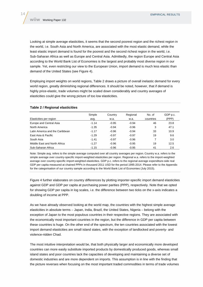
Employing import weights on world regions, Table 2 draws a picture of overall inelastic demand for every

world region, greatly diminishing regional differences. It should be noted, however, that if demand is

highly price-elastic, trade volumes might be scaled down considerably and country averages of

elasticities could give the wrong picture of too low elasticities.

Table 2 / Regional elasticities

Elasticities per region

Simple

avg.

Country

w.a.

Regional

w.a.

No. of

countries

GDP p.c.

(PPP)

Europe and Central Asia -1.14 -0.95 -0.94 46 23.8

North America -1.35 -0.94 -0.96 3 47.1

Latin America and the Caribbean -1.17 -0.96 -0.94 33 10.9

East Asia & Pacific -1.29 -0.97 -0.97 19 9.6

South Asia -1.41 -0.97 -0.96 7 3.0

Middle East and North Africa -1.27 -0.96 -0.95 19 12.5

Sub-Saharan Africa -1.15 -0.96 -0.95 41 2.6

Note: Simple avg. refers to the simple average computed over all country averages per region. Country w.a. refers to the simple average over country-specific import-weighted elasticities per region. Regional w.a. refers to the import-weighted average over country-specific import-weighted elasticities. GDP p.c. refers to the regional average expenditure-side real GDP per capita measured at chained PPPs in thousand 2011 USD for the period 1995-2014. Please refer to the Appendix for the categorisation of our country sample according to the World Bank List of Economies (July 2015).

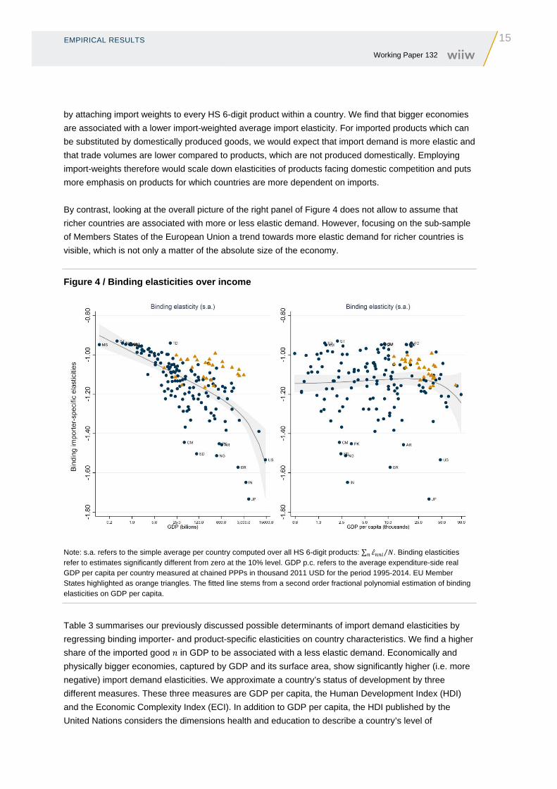
Figure 4 further elaborates on country differences by plotting importer-specific import demand elasticities

against GDP and GDP per capita at purchasing power parities (PPP), respectively. Note that we opted

for showing GDP per capita in log scales, i.e. the difference between two ticks on the x-axis indicates a

doubling of income at PPP.

As we have already observed looking at the world map, the countries with the highest simple average

elasticities in absolute terms – Japan, India, Brazil, the United States, Nigeria – belong with the

exception of Japan to the most populous countries in their respective regions. They are associated with

the economically most important countries in the region, but the difference in GDP per capita between

these countries is huge. On the other end of the spectrum, the ten countries associated with the lowest

import demand elasticities are small island states, with the exception of landlocked and poverty- and

violence-ridden Chad.

The most intuitive interpretation would be, that both physically larger and economically more developed

countries can more easily substitute imported products by domestically produced goods, whereas small

island states and poor countries lack the capacities of developing and maintaining a diverse set of

domestic industries and are more dependent on imports. This assumption is in line with the finding that

the picture reverses when focusing on the most important traded commodities in terms of trade volumes

EMPIRICAL RESULTS


by attaching import weights to every HS 6-digit product within a country. We find that bigger economies

are associated with a lower import-weighted average import elasticity. For imported products which can

be substituted by domestically produced goods, we would expect that import demand is more elastic and

that trade volumes are lower compared to products, which are not produced domestically. Employing

import-weights therefore would scale down elasticities of products facing domestic competition and puts

more emphasis on products for which countries are more dependent on imports.

By contrast, looking at the overall picture of the right panel of Figure 4 does not allow to assume that

richer countries are associated with more or less elastic demand. However, focusing on the sub-sample

of Members States of the European Union a trend towards more elastic demand for richer countries is

visible, which is not only a matter of the absolute size of the economy.

Figure 4 / Binding elasticities over income

Note: s.a. refers to the simple average per country computed over all HS 6-digit products: ∑ ⁄ . Binding elasticities refer to estimates significantly different from zero at the 10% level. GDP p.c. refers to the average expenditure-side real GDP per capita per country measured at chained PPPs in thousand 2011 USD for the period 1995-2014. EU Member States highlighted as orange triangles. The fitted line stems from a second order fractional polynomial estimation of binding elasticities on GDP per capita.

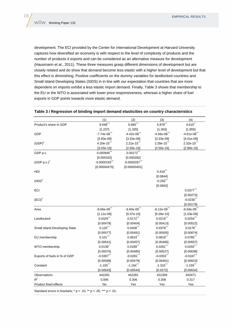
Table 3 summarises our previously discussed possible determinants of import demand elasticities by

regressing binding importer- and product-specific elasticities on country characteristics. We find a higher

share of the imported good in GDP to be associated with a less elastic demand. Economically and

physically bigger economies, captured by GDP and its surface area, show significantly higher (i.e. more

negative) import demand elasticities. We approximate a country’s status of development by three

different measures. These three measures are GDP per capita, the Human Development Index (HDI)

and the Economic Complexity Index (ECI). In addition to GDP per capita, the HDI published by the

United Nations considers the dimensions health and education to describe a country’s level of


development. The ECI provided by the Center for International Development at Harvard University

captures how diversified an economy is with respect to the level of complexity of products and the

number of products it exports and can be considered as an alternative measure for development

(Hausmann et al., 2011). These three measures grasp different dimensions of development but are

closely related and do show that demand become less elastic with a higher level of development but that

this effect is diminishing. Positive coefficients on the dummy variables for landlocked countries and

Small Island Developing States (SIDS) in in line with our expectation that countries that are more

dependent on imports exhibit a less elastic import demand. Finally, Table 3 shows that membership to

the EU or the WTO is associated with lower price responsiveness, whereas a higher share of fuel

exports in GDP points towards more elastic demand.

Table 3 / Regression of binding import demand elasticities on country characteristics

(1) (2) (3) (4)

Product's share in GDP 9.048*** 5.685*** 5.878*** 4.615**

[1.237] [1.335] [1.363] [1.855]

GDP -7.74e-08*** -4.42e-08*** -4.56e-08*** -4.61e-08***

[3.93e-09] [3.33e-09] [3.33e-09] [4.01e-09]

(GDP)2 4.20e-15*** 2.21e-15*** 2.28e-15*** 2.32e-15***

[3.03e-16] [2.56e-16] [2.56e-16] [2.89e-16]

GDP p.c. 0.000945*** 0.00172***

[0.000332] [0.000282]

(GDP p.c.)2 -0.0000193*** -0.0000267***

[0.00000475] [0.00000401]

HDI 0.418***

[0.0844]

(HDI)2 -0.259***

[0.0663]

ECI 0.0377***

[0.00273]

(ECI)2 -0.0230***

[0.00179]

Area -8.66e-09*** -6.60e-09*** -6.12e-09*** -6.63e-09***

[1.11e-09] [9.37e-10] [9.39e-10] [1.03e-09]

Landlocked 0.0329*** 0.0172*** 0.0219*** 0.0254***

[0.00479] [0.00404] [0.00413] [0.00522]

Small Island Developing State 0.120*** 0.0408*** 0.0379*** 0.0178**

[0.00577] [0.00491] [0.00505] [0.00874]

EU membership 0.101*** 0.0819*** 0.0818*** 0.0785***

[0.00541] [0.00457] [0.00466] [0.00557]

WTO membership 0.0139** 0.0189*** 0.0261*** 0.0292***

[0.00575] [0.00485] [0.00527] [0.00638]

Exports of fuels in % of GDP -0.0307*** -0.0281*** -0.0353*** -0.0167***

[0.00568] [0.00479] [0.00461] [0.00623]

Constant -1.155*** -1.164*** -1.316*** -1.159***

[0.00643] [0.00544] [0.0272] [0.00634]

Observations 442281 442281 431369 343471

R2 0.006 0.306 0.308 0.317

Product fixed effects No Yes Yes Yes

Standard errors in brackets; * p < .10, ** p < .05, *** p < .01.

EMPIRICAL RESULTS


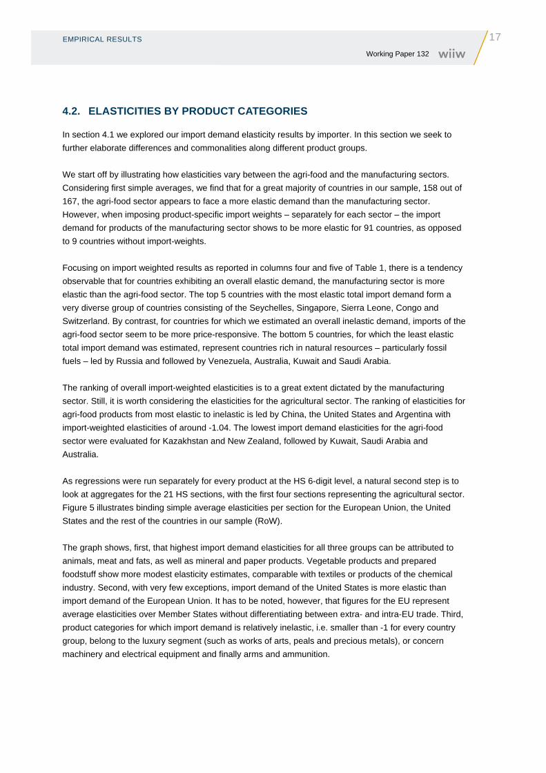
4.2. ELASTICITIES BY PRODUCT CATEGORIES

In section 4.1 we explored our import demand elasticity results by importer. In this section we seek to

further elaborate differences and commonalities along different product groups.

We start off by illustrating how elasticities vary between the agri-food and the manufacturing sectors.

Considering first simple averages, we find that for a great majority of countries in our sample, 158 out of

167, the agri-food sector appears to face a more elastic demand than the manufacturing sector.

However, when imposing product-specific import weights – separately for each sector – the import

demand for products of the manufacturing sector shows to be more elastic for 91 countries, as opposed

to 9 countries without import-weights.

Focusing on import weighted results as reported in columns four and five of Table 1, there is a tendency

observable that for countries exhibiting an overall elastic demand, the manufacturing sector is more

elastic than the agri-food sector. The top 5 countries with the most elastic total import demand form a

very diverse group of countries consisting of the Seychelles, Singapore, Sierra Leone, Congo and

Switzerland. By contrast, for countries for which we estimated an overall inelastic demand, imports of the

agri-food sector seem to be more price-responsive. The bottom 5 countries, for which the least elastic

total import demand was estimated, represent countries rich in natural resources – particularly fossil

fuels – led by Russia and followed by Venezuela, Australia, Kuwait and Saudi Arabia.

The ranking of overall import-weighted elasticities is to a great extent dictated by the manufacturing

sector. Still, it is worth considering the elasticities for the agricultural sector. The ranking of elasticities for

agri-food products from most elastic to inelastic is led by China, the United States and Argentina with

import-weighted elasticities of around -1.04. The lowest import demand elasticities for the agri-food

sector were evaluated for Kazakhstan and New Zealand, followed by Kuwait, Saudi Arabia and

Australia.

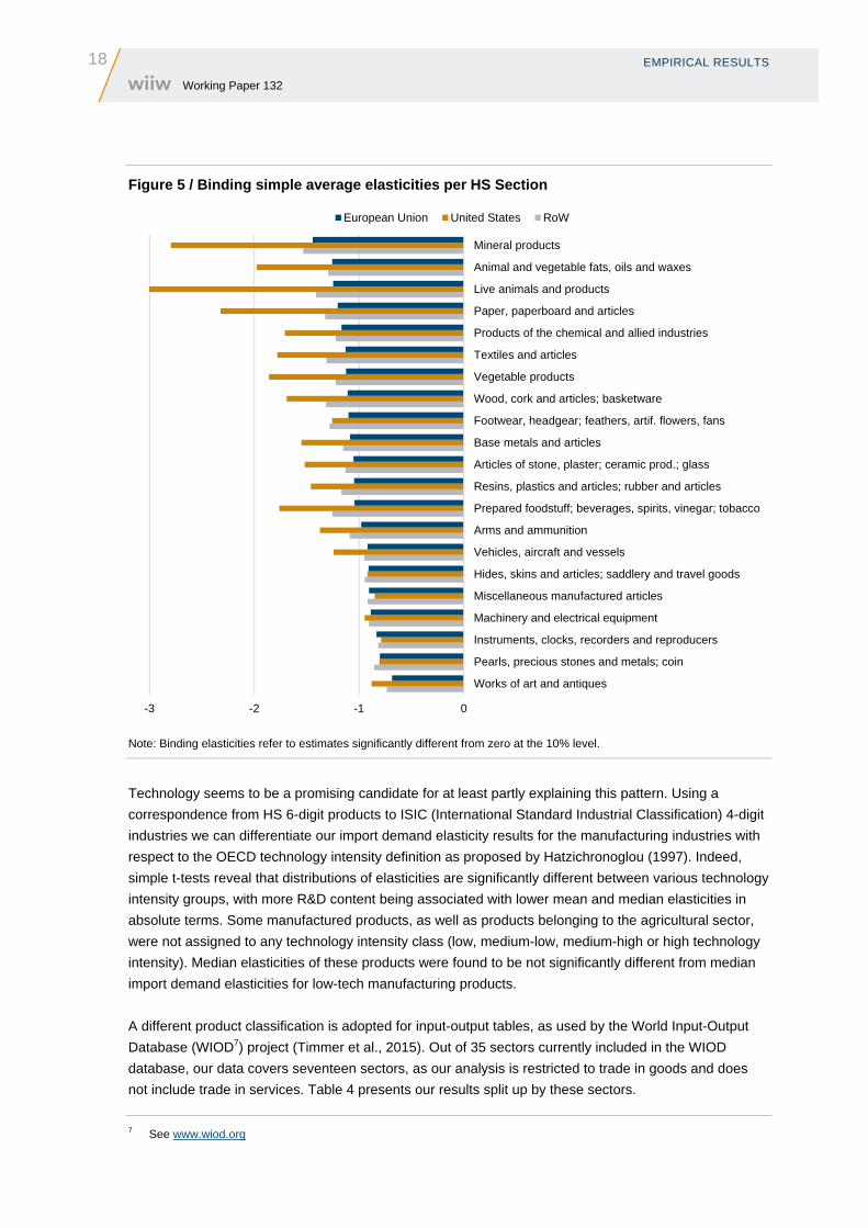
As regressions were run separately for every product at the HS 6-digit level, a natural second step is to

look at aggregates for the 21 HS sections, with the first four sections representing the agricultural sector.

Figure 5 illustrates binding simple average elasticities per section for the European Union, the United

States and the rest of the countries in our sample (RoW).

The graph shows, first, that highest import demand elasticities for all three groups can be attributed to

animals, meat and fats, as well as mineral and paper products. Vegetable products and prepared

foodstuff show more modest elasticity estimates, comparable with textiles or products of the chemical

industry. Second, with very few exceptions, import demand of the United States is more elastic than

import demand of the European Union. It has to be noted, however, that figures for the EU represent

average elasticities over Member States without differentiating between extra- and intra-EU trade. Third,

product categories for which import demand is relatively inelastic, i.e. smaller than -1 for every country

group, belong to the luxury segment (such as works of arts, peals and precious metals), or concern

machinery and electrical equipment and finally arms and ammunition.


Figure 5 / Binding simple average elasticities per HS Section

Note: Binding elasticities refer to estimates significantly different from zero at the 10% level.

Technology seems to be a promising candidate for at least partly explaining this pattern. Using a

correspondence from HS 6-digit products to ISIC (International Standard Industrial Classification) 4-digit

industries we can differentiate our import demand elasticity results for the manufacturing industries with

respect to the OECD technology intensity definition as proposed by Hatzichronoglou (1997). Indeed,

simple t-tests reveal that distributions of elasticities are significantly different between various technology

intensity groups, with more R&D content being associated with lower mean and median elasticities in

absolute terms. Some manufactured products, as well as products belonging to the agricultural sector,

were not assigned to any technology intensity class (low, medium-low, medium-high or high technology

intensity). Median elasticities of these products were found to be not significantly different from median

import demand elasticities for low-tech manufacturing products.

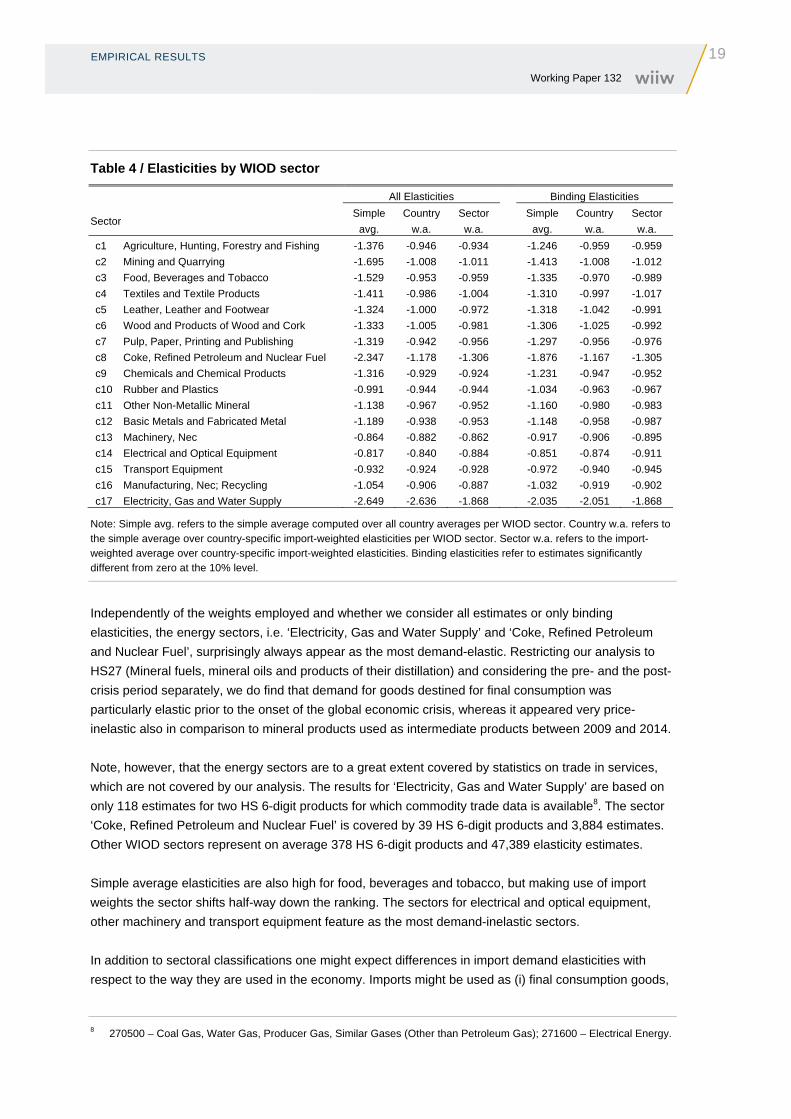
A different product classification is adopted for input-output tables, as used by the World Input-Output

Database (WIOD7) project (Timmer et al., 2015). Out of 35 sectors currently included in the WIOD

database, our data covers seventeen sectors, as our analysis is restricted to trade in goods and does

not include trade in services. Table 4 presents our results split up by these sectors.

7 See www.wiod.org

-3 -2 -1 0

Works of art and antiques

Pearls, precious stones and metals; coin

Instruments, clocks, recorders and reproducers

Machinery and electrical equipment

Miscellaneous manufactured articles

Hides, skins and articles; saddlery and travel goods

Vehicles, aircraft and vessels

Arms and ammunition

Prepared foodstuff; beverages, spirits, vinegar; tobacco

Resins, plastics and articles; rubber and articles

Articles of stone, plaster; ceramic prod.; glass

Base metals and articles

Footwear, headgear; feathers, artif. flowers, fans

Wood, cork and articles; basketware

Vegetable products

Textiles and articles

Products of the chemical and allied industries

Paper, paperboard and articles

Live animals and products

Animal and vegetable fats, oils and waxes

Mineral products

European Union United States RoW

EMPIRICAL RESULTS


Table 4 / Elasticities by WIOD sector

All Elasticities Binding Elasticities

Sector Simple

avg.

Country

w.a.

Sector

w.a.

Simple

avg.

Country

w.a.

Sector

w.a.

c1 Agriculture, Hunting, Forestry and Fishing -1.376 -0.946 -0.934 -1.246 -0.959 -0.959

c2 Mining and Quarrying -1.695 -1.008 -1.011 -1.413 -1.008 -1.012

c3 Food, Beverages and Tobacco -1.529 -0.953 -0.959 -1.335 -0.970 -0.989

c4 Textiles and Textile Products -1.411 -0.986 -1.004 -1.310 -0.997 -1.017

c5 Leather, Leather and Footwear -1.324 -1.000 -0.972 -1.318 -1.042 -0.991

c6 Wood and Products of Wood and Cork -1.333 -1.005 -0.981 -1.306 -1.025 -0.992

c7 Pulp, Paper, Printing and Publishing -1.319 -0.942 -0.956 -1.297 -0.956 -0.976

c8 Coke, Refined Petroleum and Nuclear Fuel -2.347 -1.178 -1.306 -1.876 -1.167 -1.305

c9 Chemicals and Chemical Products -1.316 -0.929 -0.924 -1.231 -0.947 -0.952

c10 Rubber and Plastics -0.991 -0.944 -0.944 -1.034 -0.963 -0.967

c11 Other Non-Metallic Mineral -1.138 -0.967 -0.952 -1.160 -0.980 -0.983

c12 Basic Metals and Fabricated Metal -1.189 -0.938 -0.953 -1.148 -0.958 -0.987

c13 Machinery, Nec -0.864 -0.882 -0.862 -0.917 -0.906 -0.895

c14 Electrical and Optical Equipment -0.817 -0.840 -0.884 -0.851 -0.874 -0.911

c15 Transport Equipment -0.932 -0.924 -0.928 -0.972 -0.940 -0.945

c16 Manufacturing, Nec; Recycling -1.054 -0.906 -0.887 -1.032 -0.919 -0.902

c17 Electricity, Gas and Water Supply -2.649 -2.636 -1.868 -2.035 -2.051 -1.868

Note: Simple avg. refers to the simple average computed over all country averages per WIOD sector. Country w.a. refers to the simple average over country-specific import-weighted elasticities per WIOD sector. Sector w.a. refers to the import-weighted average over country-specific import-weighted elasticities. Binding elasticities refer to estimates significantly different from zero at the 10% level.

Independently of the weights employed and whether we consider all estimates or only binding

elasticities, the energy sectors, i.e. ‘Electricity, Gas and Water Supply’ and ‘Coke, Refined Petroleum

and Nuclear Fuel’, surprisingly always appear as the most demand-elastic. Restricting our analysis to

HS27 (Mineral fuels, mineral oils and products of their distillation) and considering the pre- and the post-

crisis period separately, we do find that demand for goods destined for final consumption was

particularly elastic prior to the onset of the global economic crisis, whereas it appeared very price-

inelastic also in comparison to mineral products used as intermediate products between 2009 and 2014.

Note, however, that the energy sectors are to a great extent covered by statistics on trade in services,

which are not covered by our analysis. The results for ‘Electricity, Gas and Water Supply’ are based on

only 118 estimates for two HS 6-digit products for which commodity trade data is available8. The sector

‘Coke, Refined Petroleum and Nuclear Fuel’ is covered by 39 HS 6-digit products and 3,884 estimates.

Other WIOD sectors represent on average 378 HS 6-digit products and 47,389 elasticity estimates.

Simple average elasticities are also high for food, beverages and tobacco, but making use of import

weights the sector shifts half-way down the ranking. The sectors for electrical and optical equipment,

other machinery and transport equipment feature as the most demand-inelastic sectors.

In addition to sectoral classifications one might expect differences in import demand elasticities with

respect to the way they are used in the economy. Imports might be used as (i) final consumption goods,

8 270500 – Coal Gas, Water Gas, Producer Gas, Similar Gases (Other than Petroleum Gas); 271600 – Electrical Energy.


(ii) intermediate goods in the production process of final goods, or (iii) by firms in the form of stocks or

gross fixed capital formation (GFCF).

This analysis is particularly interesting in today’s context of a global trade slowdown, or even ‘trade

plateau’ (Evenett and Fritz, 2016), and negotiations of mega-regional trade deals in which non-tariff

measures play a prominent role. Every year during the period 1995-2014 imports of intermediates

represented more than 52% of global imports. The importance of global value chains as exemplified by

intermediate goods trade is increasing over time, with only three major setbacks in 1998, in 2009

following the global economic and financial crisis and in 2014.

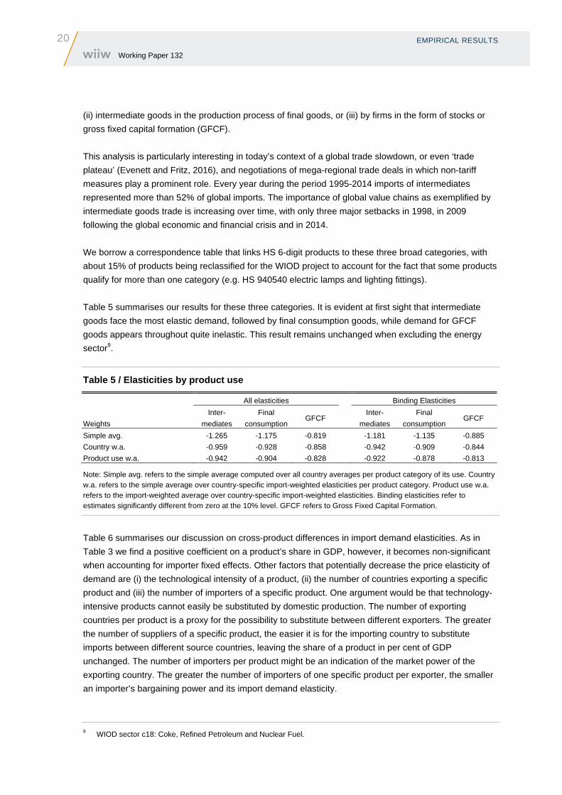
We borrow a correspondence table that links HS 6-digit products to these three broad categories, with

about 15% of products being reclassified for the WIOD project to account for the fact that some products

qualify for more than one category (e.g. HS 940540 electric lamps and lighting fittings).

Table 5 summarises our results for these three categories. It is evident at first sight that intermediate

goods face the most elastic demand, followed by final consumption goods, while demand for GFCF

goods appears throughout quite inelastic. This result remains unchanged when excluding the energy

sector9.

Table 5 / Elasticities by product use

All elasticities Binding Elasticities

Weights

Inter-

mediates

Final

consumption GFCF

Inter-

mediates

Final

consumption GFCF

Simple avg. -1.265 -1.175 -0.819 -1.181 -1.135 -0.885

Country w.a. -0.959 -0.928 -0.858 -0.942 -0.909 -0.844

Product use w.a. -0.942 -0.904 -0.828 -0.922 -0.878 -0.813

Note: Simple avg. refers to the simple average computed over all country averages per product category of its use. Country w.a. refers to the simple average over country-specific import-weighted elasticities per product category. Product use w.a. refers to the import-weighted average over country-specific import-weighted elasticities. Binding elasticities refer to estimates significantly different from zero at the 10% level. GFCF refers to Gross Fixed Capital Formation.

Table 6 summarises our discussion on cross-product differences in import demand elasticities. As in

Table 3 we find a positive coefficient on a product’s share in GDP, however, it becomes non-significant

when accounting for importer fixed effects. Other factors that potentially decrease the price elasticity of

demand are (i) the technological intensity of a product, (ii) the number of countries exporting a specific

product and (iii) the number of importers of a specific product. One argument would be that technology-

intensive products cannot easily be substituted by domestic production. The number of exporting

countries per product is a proxy for the possibility to substitute between different exporters. The greater

the number of suppliers of a specific product, the easier it is for the importing country to substitute

imports between different source countries, leaving the share of a product in per cent of GDP

unchanged. The number of importers per product might be an indication of the market power of the

exporting country. The greater the number of importers of one specific product per exporter, the smaller

an importer’s bargaining power and its import demand elasticity.

9 WIOD sector c18: Coke, Refined Petroleum and Nuclear Fuel.

EMPIRICAL RESULTS


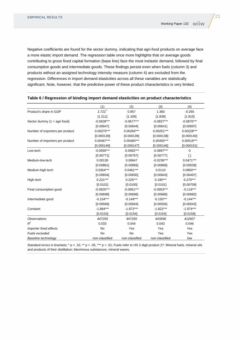
Negative coefficients are found for the sector dummy, indicating that agri-food products on average face

a more elastic import demand. The regression table once more highlights that on average goods

contributing to gross fixed capital formation (base line) face the most inelastic demand, followed by final

consumption goods and intermediate goods. These findings persist even when fuels (column 3) and

products without an assigned technology intensity measure (column 4) are excluded from the

regression. Differences in import demand elasticities across all these variables are statistically

significant. Note, however, that the predictive power of these product characteristics is very limited.

Table 6 / Regression of binding import demand elasticities on product characteristics

(1) (2) (3) (4)

Product's share in GDP 2.722** 0.957 1.360 -0.265

[1.211] [1.206] [1.839] [1.815]

Sector dummy (1 = agri-food) -0.0628*** -0.0677*** -0.0837*** -0.0870***

[0.00647] [0.00644] [0.00641] [0.00697]

Number of exporters per product 0.00270*** 0.00260*** 0.00251*** 0.00228***

[0.000139] [0.000139] [0.000138] [0.000140]

Number of importers per product 0.00467*** 0.00460*** 0.00455*** 0.00519***

[0.000146] [0.000147] [0.000146] [0.000151]

Low-tech -0.0555*** -0.0582*** -0.0897*** 0

[0.00771] [0.00767] [0.00777] [.]

Medium-low-tech 0.00130 0.00647 -0.0236*** 0.0471***

[0.00861] [0.00856] [0.00868] [0.00539]

Medium-high-tech 0.0354*** 0.0461*** 0.0110 0.0850***

[0.00834] [0.00830] [0.00843] [0.00497]

High-tech 0.221*** 0.225*** 0.190*** 0.270***

[0.0101] [0.0100] [0.0101] [0.00709]

Final consumption good -0.0925*** -0.0951*** -0.0953*** -0.119***

[0.00698] [0.00696] [0.00686] [0.00682]

Intermediate good -0.154*** -0.149*** -0.150*** -0.144***

[0.00566] [0.00564] [0.00556] [0.00543]

Constant -1.884*** -1.872*** -1.822*** -1.974***

[0.0153] [0.0154] [0.0154] [0.0159]

Observations 447259 447259 443596 412607

R2 0.033 0.044 0.043 0.046

Importer fixed effects No Yes Yes Yes

Fuels excluded No No Yes Yes

Baseline technology non-classified non-classified non-classified low

Standard errors in brackets; * p < .10, ** p < .05, *** p < .01; Fuels refer to HS 2-digit product 27: Mineral fuels, mineral oils and products of their distillation; bituminous substances; mineral waxes.

22 ROBUSTNESS Working Paper 132

5. Robustness

In the robustness section we challenge our findings10 by (i) using unconstrained import data,

(ii) performing separate regressions for the pre- and the post-crisis period, and finally by (iii) running

separate regressions for four income groups as classified by the World Bank.

5.1. THRESHOLDS FOR IMPORT DATA

Our benchmark specification does not consider observations for products that never exceeded an import

value of 10,000 USD for an importer during 1995 and 2014. The reason is that we do not want to bias

our results with economically unimportant trade flows. However, using a too high threshold for imports

might substantially decrease the number of importing countries in our sample for which elasticities can

be computed, especially small island states. The threshold of 10,000 USD is arguably somewhat

arbitrary. We therefore perform our robustness analysis for all reported import data without any

restrictions, but bearing the risk of greater outlier values in mind.

Using all reported data without dropping observations with economically seemingly low import values,

the number of initial fixed effects estimates would increase from 687,927 to 785,290 (i.e. by 14%). After

correcting estimates for endogeneity and a possible selection bias as well as dropping the tails of the

distribution and positive elasticity estimates, the final number of import demand elasticity estimates

increases from 548,625 to 603,433 estimates (i.e. by roughly 10%). This means that not employing any

restrictions on import values leaves us with a greater proportion of positive import demand elasticities to

be excluded from our analysis.

79% of the final estimates are found to be statistically significant at the 10% level, which is slightly less

than in our preferred specification. Although median values are very similar, showing inelastic import

demand elasticities of around -0.95, mean values do differ. Using all import data the minimum value, i.e.

for the most elastic product, is found at -99. This means that a 1% increase in the price of the imported

good leads to a 99% decrease in import quantities. Excluding import values below 10,000 USD reduces

this minimum value to -25. The scaling up of import demand elasticities when including smaller import

values is what we expect, recalling from equation (16) that ⁄ 1 with being a

product-specific term that is equal for all countries.

5.2. THE DIFFERENCE BETWEEN PRE- AND POST-CRISIS ESTIMATES

Our investigation encompasses data from 1995 to 2014. This period notably includes the world financial

and economic crisis, which might have had a significant impact on the elasticity of demand for imported

products. Therefore, we split our sample into a pre-crisis period covering the years 1995-2007 and a

post-crisis period 2009-2014 and estimated elasticities separately for both time spans.

10 Based on FE estimation before correction for endogeneity and self-selection.

ROBUSTNESS


Comparing results for the pre-crisis with the post-crisis period, we still find a rather inelastic mean

elasticity of -0.95 for both subsamples. However, while the mean elasticity for the pre-crisis period is

found at around -1.7, the post-2008 period shows a higher mean elasticity of -2.4. We find that the

discrepancy in mean elasticities between the pre- and post-crisis period is particularly strong for

intermediate products. Looking at simple average binding elasticities, we find demand for imports of

intermediate goods to be 13% more elastic in the post-2008 period compared to the period in the run-up

to the financial crisis. Demand for goods attributable to GFCF also appears slightly more elastic for the

post-crisis period, by roughly 1.2%, but remains rather inelastic with an average elasticity around -0.87.

Only the demand for final consumption goods shows a 1.7% lower average elasticity after the crisis.

5.3. DIFFERENTIATION BY THE LEVEL OF ECONOMIC DEVELOPMENT

The GDP function approach proposed by Kee et al. (2008) assumes that the GDP function is common

across all countries up to a country-specific term. This implies that in equation (11) which captures

the change in the share of good in GDP resulting from a price increase of good by 1% is equal

across countries.

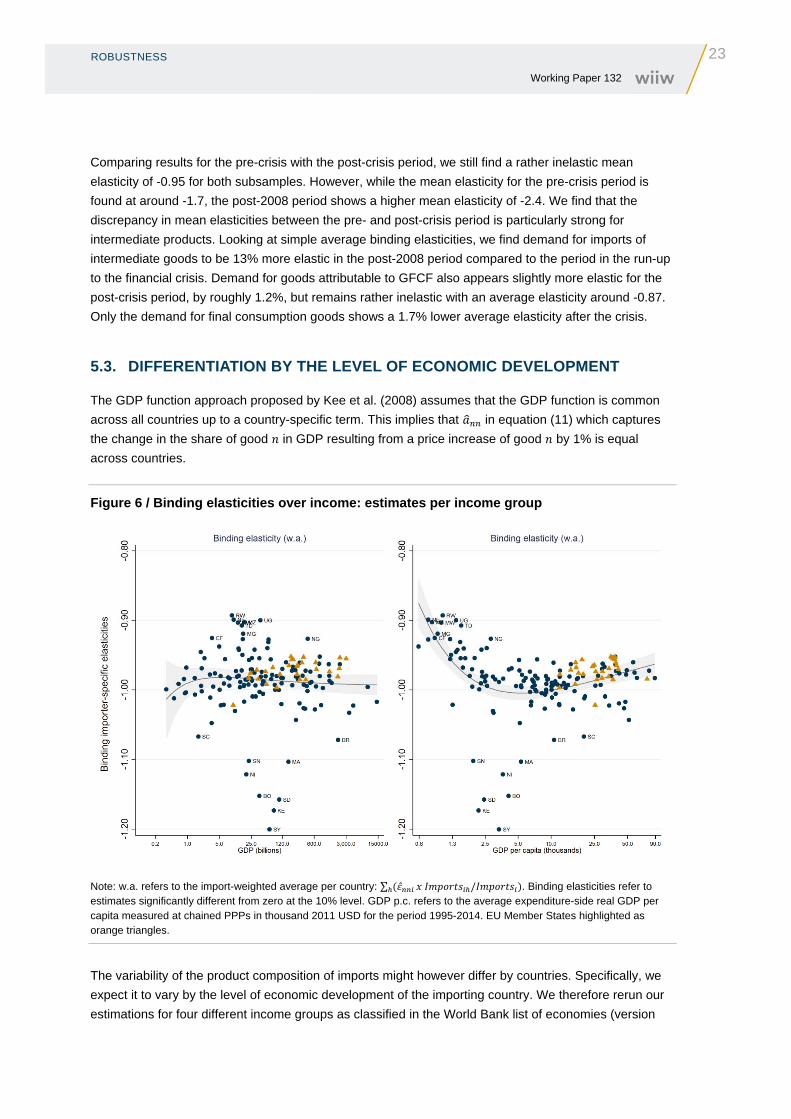
Figure 6 / Binding elasticities over income: estimates per income group

Note: w.a. refers to the import-weighted average per country: ∑ / . Binding elasticities refer to estimates significantly different from zero at the 10% level. GDP p.c. refers to the average expenditure-side real GDP per capita measured at chained PPPs in thousand 2011 USD for the period 1995-2014. EU Member States highlighted as orange triangles.

The variability of the product composition of imports might however differ by countries. Specifically, we

expect it to vary by the level of economic development of the importing country. We therefore rerun our

estimations for four different income groups as classified in the World Bank list of economies (version

24 ROBUSTNESS Working Paper 132

July 2015): (i) low-income, (ii) lower-middle-income, (iii) upper-middle-income and (iv) high-income

groups.11 The results are shown in Figure 6.

This specification improves the fit for binding elasticity estimates plotted against GDP per capita in the

right panel. In particular, the poorest countries in our sample seem to be most price-inelastic with

respect to imports, with middle-income countries being centred on an elasticity of -1 and high-income

countries again showing less elastic demand. Middle-income countries showing elasticities greater than

-1.1 comprise Syria, Kenia, Sudan, Bolivia, Nicaragua, Senegal, and Morocco.

11 For the determination of income group thresholds and data on their evolution over time please consult: https://datahelpdesk.worldbank.org/knowledgebase/articles/378833-how-are-the-income-group-thresholds-determined

CONCLUSION


6. Conclusion

In this paper, we present import demand elasticities estimated for 167 countries and 5124 products at

the six-digit level of the Harmonised System revision 1996. Following the semiflexible translog GDP

function approach proposed by Kee et al. (2008), we estimate unilateral import demand elasticities for

the period 1996-2014. Estimates by Kee et al. (2008) cover 117 countries for about 4900 products at the

HS 6-digit level. This paper constitutes an update of their work for the more recent period 1996-2014.

Improved data availability and the inclusion of products not considered in HS revision 1988 allow us to

estimate about twice as many import demand elasticities. The presented results are differentiated by

country and product characteristics.

Looking at the geographical distribution of import demand elasticities, simple averages indicate that

South Asia and North America are associated with the most elastic import demand. Countries exhibiting

the highest average elasticities belong to the economically most important countries in their respective

regions, while countries with the lowest import demand elasticities are small island states with the

exception of landlocked and poverty-ridden Chad. Import-weighted results suggest that especially

countries rich in natural resources – particularly fossil fuels – are facing an inelastic import demand, with

the agri-food sector for these states being more price-responsive than the manufacturing sector. Europe,

too, is characterised by a rather inelastic import demand, particularly for Eastern European countries

and the Iberian Peninsula.

Both the European Union and the United States show the highest elasticities for live animals, animal and

vegetable fats and mineral products, but with the United States facing an import demand about twice as

elastic. Inelastic demand is found for luxury goods such as pearls or works of art, machinery and

electrical equipment, arms and ammunition and in the case of the EU but not the US for vehicles and

aircrafts. Applying the product classification according to industries used in the WIOD, the energy

sectors again feature as the most elastic, while imports of electrical equipment and machinery are found

to be price-inelastic. Distinguishing between the use of products, it is evident that intermediate goods

face the highest elasticities, which appears particularly noteworthy in the context of an increasing

importance of global value chains and production fragmentation, the global trade slowdown since 2011

and ongoing negotiations of mega-regional trade deals.

Our preferred specification does not include importer-product observations where imports of a particular

product to one specific importer never exceeded 10,000 USD between 1995 and 2014. Using all data

provided by UN Comtrade without any import threshold has no impact on the median of the distribution

but results in higher mean elasticities with the minimum elasticity shifting from about -25 to -99. Splitting

the period 1995-2014 into a pre- and post-crisis period indicates that after 2008 import demand became

more elastic, particularly for intermediate goods. A final specification suggests that allowing the effect of

prices on the product composition of GDP to vary by the economic development of countries along the

income group classification of the World Bank, suggests that import demand elasticity is U-shaped. The

poorest countries seem to be the least price-responsive with respect to imports, while the majority of

middle-income countries is centred around unitary elasticity, with richer countries again being less

sensitive to price changes.

26 REFERENCES Working Paper 132

7. References

Altinay, G. (2007), ‘Short-run and long-run elasticities of import demand for crude oil in Turkey’, Energy Policy,

Vol. 35, pp. 5829-5835.

Beghin, J., A.-C. Disdier and S. Marette (2015), ‘Trade Restrictiveness Indices in Presence of Externalities:

An Application to Non-Tariff Measures’, Canadian Journal of Economics, Vol. 48, No. 4, November,

pp. 1513-1536.

Bratt, M. (2014), ‘Estimating the bilateral impact of non-tariff measures (NTMs)’, Working Paper WPS 14-01-1,

Université de Genève.

Broda, C. and D.E. Weinstein (2006), ‘Globalization and the gains from variety’, The Quarterly Journal of

Economics, Vol. 121, No. 2, pp. 541-585.

Caves, D.W., L.R. Christensen and W.E. Diewert (1982), ‘Multilateral comparisons of output, input, and

productivity using superlative index numbers’, The Economic Journal, Vol. 92, No. 365, March, pp. 73-86.

Diewert, W.E. and T.J. Wales (1988), ‘A normalized quadratic semiflexible functional form’, Journal of

Econometrics, Vol. 37, No. 3, pp. 327-342.

Evenett, S.J. and J. Fritz (2016), Global Trade Plateaus. The 19th Global Trade Alert Report, CEPR Press,

London.

Feenstra, R.C. and J. Romalis (2014), ‘International Prices and Endogenous Quality’, The Quarterly Journal of

Economics, Vol. 129, No. 2, May, pp. 477-527.

Feenstra, R.C., R. Inklaar and M.P. Timmer (2015), ‘The Next Generation of the Penn World Table’, American

Economic Review, Vol. 105, No. 10, pp. 3150-3182.

Hatzichronoglou, T. (1997), ‘Revision of the High-Technology Sector and Product Classification’, OECD

Science, Technology and Industry Working Papers, No. 1997/02.

Hausmann, R., C.A. Hidalgo, S. Bustos, M. Coscia, S. Chung, J. Jimenez, A. Simoes and M. Yildirim. (2011),

The Atlas of Economic Complexity, Puritan Press, Cambridge MA.

Kee, H.L., A. Nicita and M. Olarreaga (2008), ‘Import demand elasticities and trade distortions’, The Review of

Economics and Statistics, Vol. 90, No. 4, pp. 666-682.

Kee, H.L., A. Nicita and M. Olarreaga (2009), ‘Estimating Trade Restrictiveness Indices’, The Economic

Journal, Vol. 119, pp. 172-199.

Kohli, U. (1991), Technology, Duality, and Foreign Trade: The GNP Function Approach to Modeling Imports

and Exports, The University of Michigan Press, Ann Arbor.

Maoz, Z. (2009), ‘The effects of strategic and economic interdependence on international conflict across levels

of analysis’, American Journal of Political Science, Vol. 53, No. 1, pp. 223-240.

Nizovtsev, D. and A. Skiba (2016), ‘Import Demand Elasticity and Exporter Response to Anti-Dumping Duties’,

The International Trade Journal, Vol. 30, No. 2, pp. 83-114.

Panagariya, A., S. Shah and D. Mishra (2001), ‘Demand elasticities in international trade: are they really low?’,

Journal of Development Economics, Vol. 64, pp. 313-342.

Peterson, T.M. and C.G. Thies (2014), ‘The Demand for Protectionism: Democracy, Import Elasticity, and

Trade Barriers’, International Interactions, Vol. 40, pp. 103-126.

REFERENCES


Schaffer, M.E. (2010), xtivreg2: Stata module to perform extended IV/2SLS, GMM and AC/HAC, LIML and

k-class regression for panel data models, http://ideas.repec.org/c/boc/bocode/s456501.html.

Soderbery, A. (2015), ‘Estimating import supply and demand elasticities: Analysis and implications’, Journal of

International Economics, Vol. 96, pp. 1-17.

Timmer, M.P., E. Dietzenbacher, B. Los, R. Stehrer and G.J. de Vries (2015), ‘An Illustrated User Guide to the

World Input-Output Database: the Case of Global Automotive Production’, Review of International Economics,

Vol. 23, No. 3, pp. 575-605.

28 APPENDIX Working Paper 132

Appendix

Appendix 1 / Regional classification of countries

East Asia & Pacific Europe & Central Asia (ctd.) North America 1 AU Australia 61 MK TFYR of Macedonia 117 BM Bermuda 2 BN Brunei Darussalam 62 TR Turkey 118 CA Canada 3 KH Cambodia 63 UA Ukraine 119 US United States 4 CN China 64 UK United Kingdom 5 HK China, Hong Kong SAR South Asia 6 MO China, Macao SAR Latin America & Caribbean 120 BD Bangladesh 7 FJ Fiji 65 AG Antigua and Barbuda 121 BT Bhutan 8 ID Indonesia 66 AR Argentina 122 IN India 9 JP Japan 67 AW Aruba 123 MV Maldives 10 MY Malaysia 68 BS Bahamas 124 NP Nepal 11 MN Mongolia 69 BB Barbados 125 PK Pakistan 12 MM Myanmar 70 BZ Belize 126 LK Sri Lanka 13 NZ New Zealand 71 BO Bolivia 14 PH Philippines 72 BR Brazil Sub-Saharan Africa 15 KR Republic of Korea 73 CL Chile 127 BJ Benin 16 SG Singapore 74 CO Colombia 128 BW Botswana 17 TW Taiwan 75 CR Costa Rica 129 BF Burkina Faso 18 TH Thailand 76 DM Dominica 130 BI Burundi 19 VN Viet Nam 77 DO Dominican Republic 131 CV Cabo Verde 78 EC Ecuador 132 CM Cameroon Europe & Central Asia 79 SV El Salvador 133 CF Central African Republic 20 AL Albania 80 GD Grenada 134 TD Chad 21 AM Armenia 81 GT Guatemala 135 KM Comoros 22 AT Austria 82 HN Honduras 136 CG Congo 23 AZ Azerbaijan 83 JM Jamaica 137 CI Côte d'Ivoire 24 BY Belarus 84 MX Mexico 138 ET Ethiopia 25 BE Belgium 85 MS Montserrat 139 GA Gabon 26 BA Bosnia and Herzegovina 86 NI Nicaragua 140 GM Gambia 27 BG Bulgaria 87 PA Panama 141 GH Ghana 28 HR Croatia 88 PY Paraguay 142 GN Guinea 29 CY Cyprus 89 PE Peru 143 GW Guinea-Bissau 30 CZ Czech Republic 90 KN Saint Kitts and Nevis 144 KE Kenya 31 DK Denmark 91 LC Saint Lucia 145 LS Lesotho 32 EE Estonia 92 VC St. Vincent 146 MG Madagascar 33 FI Finland and the Grenadines 147 MW Malawi 34 FR France 93 SR Suriname 148 ML Mali 35 GE Georgia 94 TT Trinidad and Tobago 149 MR Mauritania 36 DE Germany 95 TC Turks and 150 MU Mauritius 37 EL Greece Caicos Islands 151 MZ Mozambique 38 HU Hungary 96 UY Uruguay 152 NA Namibia 39 IS Iceland 97 VE Venezuela 153 NE Niger 40 IE Ireland 154 NG Nigeria 41 IT Italy Middle East & North Africa 155 RW Rwanda 42 KZ Kazakhstan 98 DZ Algeria 156 ST Sao Tome and Principe 43 KG Kyrgyzstan 99 BH Bahrain 157 SN Senegal 44 LV Latvia 100 DJ Djibouti 158 SC Seychelles 45 LT Lithuania 101 EG Egypt 159 SL Sierra Leone 46 LU Luxembourg 102 IR Iran 160 ZA South Africa 47 ME Montenegro 103 IL Israel 161 SD Sudan (Former) 48 NL Netherlands 104 JO Jordan 162 SZ Swaziland 49 NO Norway 105 KW Kuwait 163 TG Togo 50 PL Poland 106 LB Lebanon 164 TZ Tanzania 51 PT Portugal 107 MT Malta 165 UG Uganda 52 MD Republic of Moldova 108 MA Morocco 166 ZM Zambia 53 RO Romania 109 OM Oman 167 ZW Zimbabwe 54 RU Russian Federation 110 QA Qatar 55 RS Serbia 111 SA Saudi Arabia 56 SK Slovakia 112 PS State of Palestine 57 SI Slovenia 113 SY Syrian Arab Republic 58 ES Spain 114 TN Tunisia 59 SE Sweden 115 AE United Arab Emirates 60 CH Switzerland 116 YE Yemen

Note: World Bank list of economies (July 2015), Montserrat not classified by the World Bank. Information on West Bank and Gaza used for Palestine.

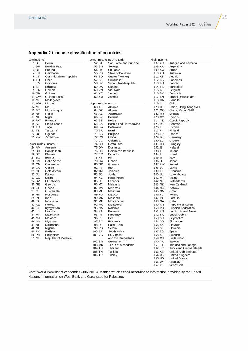
APPENDIX


Appendix 2 / Income classification of countries

Low income Lower middle income (ctd.) High income 1 BJ Benin 52 ST Sao Tome and Principe 107 AG Antigua and Barbuda 2 BF Burkina Faso 53 SN Senegal 108 AR Argentina 3 BI Burundi 54 LK Sri Lanka 109 AW Aruba 4 KH Cambodia 55 PS State of Palestine 110 AU Australia 5 CF Central African Republic 56 SD Sudan (Former) 111 AT Austria 6 TD Chad 57 SZ Swaziland 112 BS Bahamas 7 KM Comoros 58 SY Syrian Arab Republic 113 BH Bahrain 8 ET Ethiopia 59 UA Ukraine 114 BB Barbados 9 GM Gambia 60 VN Viet Nam 115 BE Belgium

10 GN Guinea 61 YE Yemen 116 BM Bermuda 11 GW Guinea-Bissau 62 ZM Zambia 117 BN Brunei Darussalam 12 MG Madagascar 118 CA Canada 13 MW Malawi Upper middle income 119 CL Chile 14 ML Mali 63 AL Albania 120 HK China, Hong Kong SAR 15 MZ Mozambique 64 DZ Algeria 121 MO China, Macao SAR 16 NP Nepal 65 AZ Azerbaijan 122 HR Croatia 17 NE Niger 66 BY Belarus 123 CY Cyprus 18 RW Rwanda 67 BZ Belize 124 CZ Czech Republic 19 SL Sierra Leone 68 BA Bosnia and Herzegovina 125 DK Denmark 20 TG Togo 69 BW Botswana 126 EE Estonia 21 TZ Tanzania 70 BR Brazil 127 FI Finland 22 UG Uganda 71 BG Bulgaria 128 FR France 23 ZW Zimbabwe 72 CN China 129 DE Germany

73 CO Colombia 130 EL Greece Lower middle income 74 CR Costa Rica 131 HU Hungary

24 AM Armenia 75 DM Dominica 132 IS Iceland 25 BD Bangladesh 76 DO Dominican Republic 133 IE Ireland 26 BT Bhutan 77 EC Ecuador 134 IL Israel 27 BO Bolivia 78 FJ Fiji 135 IT Italy 28 CV Cabo Verde 79 GA Gabon 136 JP Japan 29 CM Cameroon 80 GD Grenada 137 KW Kuwait 30 CG Congo 81 IR Iran 138 LV Latvia 31 CI Côte d'Ivoire 82 JM Jamaica 139 LT Lithuania 32 DJ Djibouti 83 JO Jordan 140 LU Luxembourg 33 EG Egypt 84 KZ Kazakhstan 141 MT Malta 34 SV El Salvador 85 LB Lebanon 142 NL Netherlands 35 GE Georgia 86 MY Malaysia 143 NZ New Zealand 36 GH Ghana 87 MV Maldives 144 NO Norway 37 GT Guatemala 88 MU Mauritius 145 OM Oman 38 HN Honduras 89 MX Mexico 146 PL Poland 39 IN India 90 MN Mongolia 147 PT Portugal 40 ID Indonesia 91 ME Montenegro 148 QA Qatar 41 KE Kenya 92 MS Montserrat 149 KR Republic of Korea 42 KG Kyrgyzstan 93 NA Namibia 150 RU Russian Federation 43 LS Lesotho 94 PA Panama 151 KN Saint Kitts and Nevis 44 MR Mauritania 95 PY Paraguay 152 SA Saudi Arabia 45 MA Morocco 96 PE Peru 153 SC Seychelles 46 MM Myanmar 97 RO Romania 154 SG Singapore 47 NI Nicaragua 98 LC Saint Lucia 155 SK Slovakia 48 NG Nigeria 99 RS Serbia 156 SI Slovenia 49 PK Pakistan 100 ZA South Africa 157 ES Spain 50 PH Philippines 101 VC St. Vincent 158 SE Sweden 51 MD Republic of Moldova and the Grenadines 159 CH Switzerland

102 SR Suriname 160 TW Taiwan 103 MK TFYR of Macedonia 161 TT Trinidad and Tobago 104 TH Thailand 162 TC Turks and Caicos Islands 105 TN Tunisia 163 AE United Arab Emirates 106 TR Turkey 164 UK United Kingdom

165 US United States 166 UY Uruguay 167 VE Venezuela

Note: World Bank list of economies (July 2015), Montserrat classified according to information provided by the United Nations. Information on West Bank and Gaza used for Palestine.

30 APPENDIX Working Paper 132

WIIW WORKING PAPERS PUBLISHED


WIIW WORKING PAPERS PUBLISHED SINCE 2013

For current updates and summaries see also wiiw's website at www.wiiw.ac.at

No. 132 Mahdi Ghodsi, Julia Grübler and Robert Stehrer: Import Demand Elasticities Revisited, November 2016

No. 131 Leon Podkaminer: Has Trade Been Driving Global Economic Growth?, October 2016

No. 130 Philipp Heimberger: Did Fiscal Consolidation Cause the Double-Dip Recession in the Euro Area?, October 2016

No. 129 Julia Grübler, Mahdi Ghodsi and Robert Stehrer: Estimating Importer-Specific Ad Valorem Equivalents of Non-Tariff Measures, September 2016

No. 128 Sebastian Leitner and Robert Stehrer: Development of Public Spending Structures in the EU Member States: Social Investment and its Impact on Social Outcomes, August 2016

No. 127 Roman Stöllinger: Structural Change and Global Value Chains in the EU, July 2016

No. 126 Jakob Kapeller, Michael Landesmann, Franz X. Mohr and Bernhard Schütz: Government Policies and Financial Crises: Mitigation, Postponement or Prevention?, May 2016

No. 125 Sandra M. Leitner and Robert Stehrer: The Role of Financial Constraints for Different Innovation Strategies: Evidence for CESEE and FSU Countries, April 2016

No. 124 Sandra M. Leitner: Choosing the Right Partner: R&D Cooperations and Innovation Success, February 2016

No. 123 Michael Landesmann, Sandra M. Leitner and Robert Stehrer: Changing Patterns in M&E-Investment-Based Innovation Strategies in CESEE and FSU Countries: From Financial Normalcy to the Global Financial Crisis, February 2016

No. 122 Sebastian Leitner: Drivers of Wealth Inequality in Euro-Area Countries. The Effect of Inheritance and Gifts on Household Gross and Net Wealth Distribution Analysed by Applying the Shapley Value Approach to Decomposition, January 2016

No. 121 Roman Stöllinger: Agglomeration and FDI: Bringing International Production Linkages into the Picture, December 2015

No. 120 Michael Landesmann and Sandra M. Leitner: Intra-EU Mobility and Push and Pull Factors in EU Labour Markets: Estimating a Panel VAR Model, August 2015

No. 119 Michael Landesmann and Sandra M. Leitner: Labour Mobility of Migrants and Natives in the European Union: An Empirical Test of the ‘Greasing of the Wheels’ Effect' of Migrants, August 2015

No. 118 Johannes Pöschl and Katarina Valkova: Welfare State Regimes and Social Determinants of Health in Europe, July 2015

No. 117 Mahdi Ghodsi: Distinguishing Between Genuine and Non-Genuine Reasons for Imposing TBTs; A Proposal Based on Cost Benefit Analysis, July 2015

No. 116 Mahdi Ghodsi: Role of Specific Trade Concerns on TBT in the Import of Products to EU, USA, and China, June 2015

No. 115 Mahdi Ghodsi: Determinants of Specific Trade Concerns Raised on Technical Barriers to Trade, June 2015

No. 114 Sandra M. Leitner and Robert Stehrer: What Determines SMEs’ Funding Obstacles to Bank Loans and Trade Credits? A Comparative Analysis of EU-15 and NMS-13 Countries, May 2015

No. 113 Sebastian Leitner: Effects of Income Inequality on Population Health and Social Outcomes at the Regional Level in the EU – Differences and Similarities between CEE and Non-CEE EU Regions, May 2015

No. 112 Arne J. Nagengast and Robert Stehrer: The Great Collapse in Value Added Trade, April 2015

No. 111 Michael Landesmann, Sandra Leitner and Isilda Mara: Should I Stay, Should I Go Back or Should I Move Further? Contrasting Answers under Diverse Migration Regimes, January 2015

No. 110 Robert Stehrer: Does the Home Bias Explain Missing Trade in Factors? December 2014

No. 109 Sebastian Leitner and Robert Stehrer: Labour Market Transitions of Young People during the Economic Crisis, November 2014

No. 108 Neil Foster-McGregor, Johannes Pöschl and Robert Stehrer: Capacities and Absorptive Barriers for International R&D Spillovers through Intermediate Inputs, October 2014

No. 107 Arne J. Nagengast and Robert Stehrer: Collateral Imbalances in Intra-European Trade? Accounting for the Differences between Gross and Value Added Trade Balances, July 2014

No. 106 Roman Stöllinger and Mario Holzner: State Aid and Export Competitiveness in the EU, December 2013

No. 105 Neil Foster-McGregor, Anders Isaksson and Florian Kaulich: Importing, Productivity and Absorptive Capacity in Sub-Saharan African Manufacturing Firms, November 2013

No. 104 Isilda Mara and Michael Landesmann: The Steadiness of Migration Plans and Expected Length of Stay – Based on a Recent Survey of Romanian Migrants in Italy, September 2013

No. 103 Isilda Mara and Michael Landesmann: Do I Stay because I am Happy or am I Happy because I Stay? Life Satisfaction in Migration, and the Decision to Stay Permanently, Return and Out-migrate, August 2013

No. 102 Rod Falvey and Neil Foster-McGregor: On the Trade and Price Effects of Preferential Trade Agreements, May 2013

IMPRESSUM

Herausgeber, Verleger, Eigentümer und Hersteller:

Verein „Wiener Institut für Internationale Wirtschaftsvergleiche“ (wiiw),

Wien 6, Rahlgasse 3

ZVR-Zahl: 329995655

Postanschrift: A 1060 Wien, Rahlgasse 3, Tel: [+431] 533 66 10, Telefax: [+431] 533 66 10 50

Internet Homepage: www.wiiw.ac.at

Nachdruck nur auszugsweise und mit genauer Quellenangabe gestattet.

Offenlegung nach § 25 Mediengesetz: Medieninhaber (Verleger): Verein "Wiener Institut für

Internationale Wirtschaftsvergleiche", A 1060 Wien, Rahlgasse 3. Vereinszweck: Analyse der

wirtschaftlichen Entwicklung der zentral- und osteuropäischen Länder sowie anderer

Transformationswirtschaften sowohl mittels empirischer als auch theoretischer Studien und ihre

Veröffentlichung; Erbringung von Beratungsleistungen für Regierungs- und Verwaltungsstellen,

Firmen und Institutionen.

wiiw.ac.at

import demand elasticities revisited - wiiw...import demand elasticities revisited mahdi ghodsi...

Documents