implicit discretization of lagrangian gas dynamics
TRANSCRIPT
HAL Id: cea-03284467https://hal-cea.archives-ouvertes.fr/cea-03284467
Preprint submitted on 12 Jul 2021
HAL is a multi-disciplinary open accessarchive for the deposit and dissemination of sci-entific research documents, whether they are pub-lished or not. The documents may come fromteaching and research institutions in France orabroad, or from public or private research centers.
L’archive ouverte pluridisciplinaire HAL, estdestinée au dépôt et à la diffusion de documentsscientifiques de niveau recherche, publiés ou non,émanant des établissements d’enseignement et derecherche français ou étrangers, des laboratoirespublics ou privés.
Implicit discretization of Lagrangian gas dynamicsA. Plessier, S. del Pino, B. Després
To cite this version:A. Plessier, S. del Pino, B. Després. Implicit discretization of Lagrangian gas dynamics. 2021. cea-03284467
Implicit discretization of Lagrangian gas dynamics
A. Plessier∗1,2, S. Del Pino1,4, and B. Després2,3
1CEA, DAM, DIF, F-91297 Arpajon, France2LJLL (UMR_7598) - Laboratoire Jacques-Louis Lions
3IUF - Institut Universitaire de France4Université Paris-Saclay, Laboratoire en Informatique Haute Performance pour le Calcul
et la simulation
July 12, 2021
Abstract
We construct an original framework based on convex analysis to prove the existence and unique-ness of a solution to a class of implicit numerical schemes. We propose an application of this generalframework in the case of a new non linear implicit scheme for the 1D Lagrangian gas dynamicsequations. We provide numerical illustrations that corroborate our proof of unconditional stabilityfor this non linear implicit scheme.
KeywordsImplicit Finite Volume Scheme, Lagrangian Formalism, Entropy Stability, Convex Analysis
1 Introduction
To approach equations traducing the movements of fluids, explicit schemes are traditionally used, see,16,29because they are easy to implement. Explicit schemes need to satisfy a stability CFL condition: c∆t 6∆x, where c is the speed of sound, ∆t is the time step, and ∆x is the size of the discretization in spaceof the mesh. The time step is constrained by the size of the smallest cell. Nevertheless, in some cases, alarge speed of sound (c 1) contributes to have such small time steps that it becomes unfavourable touse explicit methods, because the simulation cost is high.
Implicit in time schemes have always aroused interest in the literature. In particular, they are muchless sensitive to the CFL number: for example a finite difference algorithm is proposed in Beam andWarming,2 implicit and semi-implicit schemes are investigated in the Toth, Keppens and Bochev33 andan experimentation on implicit upwind methods for Euler equations is done in Mulder and Van Leer.25Some other implicit algorithms are explained in the following articles, see for example.9,24,28 A largepart of them use the method of predictor-corrector scheme like in the works.20,26,34–36 More recent workscan be found in the articles.6,27
Nonetheless, some major technical difficulties appear for the numerical resolution of implicit nonlinear schemes. At a theoretical level, it is difficult to prove the existence and uniqueness of a solution toimplicit schemes. Currently, a powerful theory is the one developed in Gallouët et al.,15 for Navier-Stokesequations with viscosity, using the topological degree. The existence of a solution is proved in details, butthe uniqueness requires restrictive hypothesis. Another strategy is explained in Brugano and Casulli3 forpiecewise linear systems in the case of a symmetrical structure. The existence of a solution is proved, andthe uniqueness is also studied in the case of special hypothesis. A non-linear implicit-explicit strategy isfound in Fryxell et al.,14 that is second order in both space and time. There are no proof of existence oruniqueness, but the numerical results illustrate an unconditional stability of the method.
1
Our original contributions to this field are, firstly the elaboration of a general framework whichallows to prove existence and uniqueness of implicit solution of some numerical schemes, and secondly theapplication of the general framework in the case of a non linear implicit scheme for the 1D model problem(1) written in semi-Lagrangian coordinates (semi-Lagrangian coordinates means Lagrange+update)
ρDtτ − ∂xu = 0,
ρDtu+ ∂xp = 0,
ρDtE + ∂xpu = 0.
(1)
One has ρ = 1τ > 0 the mass density, p is the pressure, u is the velocity and E is the total energy density.
The variables τ and p are taken positive to be physically admissible, see Serre31 or Ern and Guermond12for more details. The material derivative is Dt = ∂t+u∂x. The following set of equations is the isentropicEuler equations for the prediction step of the implicit scheme
ρDtτ − ∂xu = 0,
ρDtu+ ∂xp = 0,
ρDtS = 0.
(2)
The first two equations are identical to (1), only the last one is different, with S denoting the physicalentropy. These equations are equipped with a perfect gas equation of state
p = (γ − 1)e
τ,
e = CvT,
S = Cv log(eτγ−1),
(3)
where Cv is the thermal capacity at constant volume, γ > 1 is the adiabatic index, e = E − 12u
2 is theinternal energy density, T is the temperature and c is the speed of sound given by c2 = ∂p
∂ρ .The justification of using a prediction step based on the discretization of (2) comes from ideas in the
work of Chalons, Coquel and Marmignon.4 It will be explained in details in this article.Consider a meshM composed of N cells noted j ∈ 1, . . . , N. The time t is discretized with a time
step ∆t that corresponds to one iteration. The mass of the cell j is Mj . The boundary conditions aresupposed periodic, and the fluxes are defined with the acoustic impedance αj+ 1
2> 0. The scheme has a
predictor-corrector structure. The prediction step is written as
Prediction step
τj = τnj +
∆t
Mj(uj+ 1
2− uj− 1
2),
uj = unj −∆t
Mj(pj+ 1
2− pj− 1
2),
Sj = Snj .
(4)
The correction step is given by
Correction step
τn+1j = τnj +
∆t
Mj(uj+ 1
2− uj− 1
2),
un+1j = unj −
∆t
Mj(pj+ 1
2− pj− 1
2),
En+1j = Enj +
∆t
Mj(pj+ 1
2uj+ 1
2− pj− 1
2uj− 1
2),
(5)
where only the total energy equation is modified. The correction step is explicit so the main difficulty isin the prediction step.
In (4) and (5), the fluxes are defined by
pj − pj+ 12
= αnj+ 12(uj+ 1
2− uj), pj − pj− 1
2= αnj− 1
2(uj − uj− 1
2),
2

where the coefficient αnj+ 1
2
> 0 is for simplicity equal to a mean value of the acoustic impedance:
αj+ 12
= 12 (ρjcj + ρj+1cj+1). Another equivalent formula is
pj+ 12
=ρjcj + ρj+1cj+1
4(uj − uj+1) +
1
2(pj + pj+1),
uj+ 12
=1
ρjcj + ρj+1cj+1(pj − pj+1) +
1
2(uj + uj+1).
In Lagrangian formalism, the mesh moves according to the velocity of the fluid: xn+1j+ 1
2
= xnj+ 1
2
+ ∆tunj+ 1
2
.The predictor-corrector scheme (4-5) is naturally conservative since it is expressed in terms of fluxes.Such a scheme can be proved to be weakly consistent as in Després.10,11
The predictor-corrector scheme is an adaptation of ideas from the article4 which is dedicated to solvethe classical Euler equations (6)
∂tρ+ ∂xρu = 0,
∂tρu+ ∂x(ρu2 + p) = 0,
∂tρE + ∂x(ρEu+ pu) = 0.
(6)
The authors explain that the difficulties of solving this system come from the flux terms in the second andthird equations. Indeed, there is a strong non linearity due in particular to the pressure. To overcomethis complexity, the authors propose a predictor-corrector strategy that we use also in this work. Firstlyis to solve the isentropic Euler equations (7) during the prediction step
∂tρ+ ∂xρu = 0,
∂tρu+ ∂x(ρu2 + p) = 0,
∂tρS + ∂xρSu = 0.
(7)
Secondly, the classical Euler equations (6) are solved in order to restore the conservation of the totalenergy. At a discrete level, the fluxes are expressed thanks to an isentropic scheme, and then insertedin the scheme associated to (6). For the prediction step, the authors use a relaxation scheme on thepressure. They prove the existence of a solution to the relaxation implicit scheme. Nonetheless, therobustness of the scheme depends on an extra equation as mentionned in a report, see.30
Let us now describe our results. For physically admissible data, the system (4) will be said uncon-ditionally stable if there exists a unique solution to the implicit non-linear scheme. Our proof of theunconditional stability of (4) comes from a rewriting of the prediction step (4) under the form
Find U ∈ D such that∇J(U) = AU,
(8)
where U is a vector of real unknowns, J is a functional defined on a domain D and A is a matrix of realcoefficients.
The proof that (8) has a unique solution relies on Theorem 4 that seems to be new consideringthe classical literature of convex analysis, see.1,17,19 The ingredients to establish Theorem 4 are thefollowing.
Hypothesis 1. The open convex domain is D =]−∞, 0[n×Rm ⊂ Rn×Rm, where n > 0 and m > 0 aretwo integers. Its boundary is ∂D = V ∈ Rn+m : ∃ j∗ ∈ 1, . . . , n Vj∗ = 0, ∀j 6= j∗ ∈ 1, . . . , n, Vj 60.
We made a slight abuse of notations by using the same letter n in the Hypothesis 1 as the iterationindex in the scheme (4 -5). We believe this does not interfere with the readability. The case m = 0corresponds to the Traffic flow equations studied in the Appendix. Otherwise m = n.
Hypothesis 2. The function J : U ∈ D → J(U) ∈ R is C2, strictly convex and coercive in the sensethat
J(U)→ +∞ for ||U || −−−→U∈D
+∞. (9)
3
Moreover for all V ∈ ∂D there exists a unit direction d ∈ Rn+m which is outward from D such that
(∇J(V − εd),d)ε→0+
−−−−−−→V−εd∈D
+∞. (10)
Also for all V ∈ ∂D, one has||∇J(W )|| W→V−−−−→
W∈D+∞. (11)
The verification of (9), (10) and (11) will be obtained directly from the perfect gas law equations (3).For an isentropic gas, it can be simplified.
Hypothesis 3. The matrix A ∈Mn+m(R) is skew-symmetric and its kernel satisfies ker(A) ∩ D 6= ∅.
Theorem 4. Under the Hypothesis 1, 2 and 3, the problem (8) has a unique solution.
Applying this Theorem, we show that (4) is well defined for all ∆t > 0.
Corollary 5. Considering physically admissible data (τnj > 0 for all j), the prediction scheme (4) canbe written under the form (8). Therefore, it is unconditionally stable.
Moreover, the predictor-corrector scheme (4-5) satisfies two entropy inequalities.
Theorem 6. For all ∆t > 0, the solution of the prediction step (4) satisfies
∀j,Ej − Enj
∆t+puj+ 1
2− puj− 1
2
Mj6 0, with puj+ 1
2= pj+ 1
2uj+ 1
2. (12)
The solution of the correction step (5) verifies the entropy inequality
∀j,Sn+1j − Snj
∆t> 0. (13)
The organization of this article is as follows. In Section 2 we write the scheme (4) under the form (8).In Section 3, we prove Theorem 4. The proof is split in several parts. On the one side we rapidly provethe uniqueness of a solution, and on the other side we decompose the proof of the existence in differentsteps. In Section 4, we apply Theorem 4 for the isentropic Euler equations, and prove Corollary 5.In Section 5, the correction step is introduced and the complete scheme is fully justified. The proofof Theorem 6 concerning entropy inequalities for both steps is detailed. In Section 6, we provide afew numerical illustrations. The Appendix contains the application of Theorem 4 for the traffic flowproblem, in the specific case where m = 0 in the definition of D. It also contains a brief description ofthe modification to treat an isothermal equation of state.
2 Formulation under the form (8)
The objective of this Section is to provide the details of the transformation from the implicit scheme (4)to the form (8). The verification of Hypothesis 1, 2 and 3 will be performed in Section 4.
We consider Euler isentropic equations in one dimension (2) for compressible perfect gas with periodicboundary conditions. As the physical entropy S is constant during this prediction step, its equation isnot necessary for the proof. Replacing the fluxes and rearranging the terms in (4), one obtains
2Mj
∆t(τj − τnj ) +
1
αnj+ 1
2
(pj+1 − pj) +1
αnj− 1
2
(pj−1 − pj) = uj+1 − uj−1,
2Mj
∆t(uj − unj ) + αnj+ 1
2(uj − uj+1) + αnj− 1
2(uj − uj−1) = pj−1 − pj+1.
(14)
Let us define a vector of unknowns
U = ((−pj)j∈1,...,N, (uj)j∈1,...,N) ∈ D, (15)
4
where the domain D is defined as
D = U such that ∀j ∈ 1, . . . , N − pj < 0, and uj ∈ R . (16)
The matrix A is defined by
A =
[0 BB 0
]with B =
0 1 0 · · · 0 −1−1 0 1 0 · · · 0
0. . . . . . . . . . . .
......
. . . . . . . . . . . . 00 · · · 0 −1 0 11 0 · · · 0 −1 0
∈MN (R). (17)
The functional J : D → R is defined as a sum of elementary functions
J(U) =
N∑j=1
2Mj
∆t
[L1j (−pj) + L2
j (uj)]
+
N∑j=1
[Q1j (−pj ,−pj+1) +Q2
j (uj , uj+1)], (18)
where the elementary functions are
L1j (−p) = −Cjp1− 1
γ + τnj p, where Cj = γ(γ − 1)−1+ 1
γ exp
(SjCv
) 1γ
> 0,
Q1j (−p,−q) =
1
αj+ 12
(q − p)2
2, L2
j (u) =u2
2− unj u, Q2
j (u, v) = αj+ 12
(u− v)2
2.
Proposition 7. The calculation of a solution (τj > 0, uj)16j6N to the system (14) of scalar non-linearequations is equivalent to the calculation of a solution U ∈ D to the global non-linear equation ∇J(U) =AU .
Proof. For a perfect gas law, the correspondence between τ , p and S can be written as τ = (γ −1) exp ( S
Cv)
1γ p−
1γ . Therefore the equivalence between a solution of (14) and a solution (15) of ∇J(U) =
AU is explicited by
τj = (γ − 1) exp (SjCv
)
1γ
p− 1γ
j and uj = uj . (19)
To finish the proof it is sufficient to calculate explicitly ∇J(U). The derivatives of L1j , L2
j , Q1j and Q2
j
are∂L1
j
∂(−pj)= Cj
(γ − 1
γ
)p− 1γ
j − τnj = τj − τnj ,∂L2
j
∂uj= uj − unj ,
∂Q1j
∂(−pj)=
1
αj+ 12
(pj+1 − pj) +1
αj− 12
(pj−1 − pj),
∂Q2j
∂uj= αj+ 1
2(uj − uj+1) + αj− 1
2(uj − uj−1).
By (18), one calculates all the components of the vector ∇J(U) ∈ R2N . With the definition (17) of thematrix A, one obtains immediately that the first N equations in the vectorial identity ∇J(U) = AU are
2Mj
∆t(τj − τnj ) +
1
αnj+ 1
2
(pj+1 − pj) +1
αnj− 1
2
(pj−1 − pj) = uj+1 − uj−1, 1 6 j 6 N, (20)
while the last N equations are
2Mj
∆t(uj − unj ) + αnj+ 1
2(uj − uj+1) + αnj− 1
2(uj − uj−1) = pj−1 − pj+1, 1 6 j 6 N. (21)
With the correspondence (19), one finds that (20 -21) is equal to (14).
5
3 Proof of Theorem 4
In this Section, we prove Theorem 4 stated in the introduction under the Hypothesis 1, 2 and 3. EachSubsection corresponds to an intermediate result leading to the final outcome.In convex analysis, see e.g.[Hirriart-Urruty and Lemarechal18 Def. 3.2.5 p19], the closure of the functionJ is J , defined as
J : Rn+m →R
U 7→
limV→U
infV ∈D
J(V ) if U ∈ D,
+∞ if not.
(22)
By construction, J is lower semi-continuous because J is continuous over D. For a function J which iscoercive on its domain D like in (9), the closure J is also coercive in the sense of the book of Hirriart-Urruty,17 [Chapter 2, p 41]
J(U)→ +∞ for ||U || −−−−−−→U∈Rn+m
+∞.
3.1 UniquenessIt relies on elementary considerations.
Lemma 8. Assuming that the problem (8) admits a solution in D, then it is unique.
Proof. Let U1 ∈ D and U2 ∈ D be two solutions of the problem (8)∇J(U1) = AU1,
∇J(U2) = AU2.
One has(∇J(U1)−∇J(U2), U1 − U2) = (A(U1 − U2), U1 − U2) .
Since A is a skew-symmetric matrix therefore (A(U1 − U2), U1 − U2) = 0, that is
(∇J(U1)−∇J(U2), U1 − U2) = 0.
Since J is strictly convex, this is only satisfied if U1 = U2.
3.2 ExistenceThe existence of a solution relies on a few intermediate results.
3.2.1 Existence of a minimum for J
The first result to prove is the existence of a minimum point for the function J , using a classical resultfrom convex analysis.
Lemma 9. The function J admits a unique minimum U ∈ D.
Proof. We apply [Theorem 1.1 p 48] of Dacorogna7 to the function f = J . So there exists U ∈ Rn+m
such that J(U) 6 J(V ) for all V ∈ Rn+m. Necessarily J(U) <∞ is finite so U ∈ D. It remains to showthat U /∈ ∂D.
Let us assume on the contrary that U ∈ ∂D. Thanks to the convexity of J and inequality (10) inHypothesis 2, one can write
J(U) > J(U − εd) + ε (∇J(U − εd),d) > J(U − εd).
It is a contradiction. Therefore U ∈ D is a minimum and U is unique thanks to the strict convexity ofJ on D.
Since D is an open set, the unique minimum U ∈ D of J satisfies the Euler equation, see Hirriart-Urruty,17 [Chapter 2, p 41]
∇J(U) = 0.
6

3.2.2 A continuation method
We prove in this section that, the problem (23) admits a solution in the domain D for all 0 6 ε 6 1Find Uε ∈ D such that∇J(Uε) = εAUε.
(23)
For ε = 0, the problem is treated in Section 3.2.1. This allows to write (23) with a continuation methodunder the form of an initial value problem (24)
∇2J(Uε)dUεdε
= AUε + εAdUεdε
,
U0 = argminU∈D
J(U).(24)
A rearrangement yields (∇2J(Uε) − εA)dUεdε = AUε. For U ∈ D, the matrix ∇2J(U) − εA is invertiblethanks to the following result.
Lemma 10. Let A and B be two matrices ofMN,N (R) such that A is skew symmetric and B is positivedefinite. Then the matrix C = A+B ∈MN,N (R) is invertible.
The Lemma 10 is applied with −εA as the skew symmetric matrix, and ∇2J(Uε) as the positivedefinite matrix. Thus (∇2J(Uε)− εA)
−1 exists. The initial value problem can be rewritten asdUεdε
= (∇2J(Uε)− εA)−1AUε,
U0 = argminU∈D
J(U).
Let us define I = [0,+∞[ and the function F : I ×D → Rn+m by F (ε, V ) = (∇2J(V )− εA)−1AV . The
problem is rewritten as dUεdε
= F (ε, Uε),
U0 = argminU∈D
J(U).(25)
To obtain the existence of a maximal solution to (25), one can apply standard results from the theoryof ODEs that we recall now.
Definition 11 (see Coddington and Levinson,5 Chapter 1). Let N ∈ N and F : I × RN → RN , letε0 ∈ I, and Uε ∈ RN where I is a non empty interval of R. A solution of the differential equation
U ′(ε) = F (ε, U(ε)), (26)
is given by a non empty interval I ⊂ I and a differentiable function U : I → RN satisfying (26) for allε ∈ I.
A solution of the initial value problem (or Cauchy problem) associated to (26) is a solution of (26)such that ε0 ∈ I and U(ε0) = U0.
Theorem 12 (Cauchy Lipschitz Theorem for locally Lipschitz functions,5 Th. 3.1, p12). Let the functionF be a C1 function, then, for all initial data (ε0, U0) ∈ I ×RN , there exists an interval I ∈ I containingε0 such that there exists in I a unique solution to the associated initial value problem.
In particular for all such data, there exists a unique maximal solution and all other solution verifyingthe condition of Cauchy is a restriction of the maximal solution.
Lemma 13. There exists 0 < εmax such that for all ε ∈ [0, εmax[, the problem (25) admits a solution inD. This solution satisfies (23).
7

Proof. One applies the Cauchy Lipschitz Theorem. The function F is well defined, and differentiable interms of ε. The derivative is continuous because A is a matrix of scalar coefficients, and J is a functionof class C2 thanks to Hypothesis 2. F is then of class C1.
To prove the last part of the Lemma, one notes that
d
dε(∇J(Uε)− εAUε) = (∇2J(Uε)− εA)
d
dεUε −AUε = 0.
Since ∇J(U0) = 0 it shows that ∇J(Uε)− εAUε = 0 on the maximal interval.
In the rest of this Section, we prove that εmax > 1.
3.2.3 Upper bound of J(Uε)
In this section, the objective is to prove that J(Uε) is bounded, which is necessary to conclude that thesolution of the problem (23) stays in the domain D.
Lemma 14. There exists U ∈ D such that the following inequality is satisfied on the maximal interval
J(Uε) 6 J(U) < +∞.
Proof. Let us take U ∈ ker(A) ∩ D that is non empty by Hypothesis 3. The convexity of J implies that
J(Uε) + (∇J(Uε), U − Uε) 6 J(U).
One findsJ(Uε) + (εAUε, U)− (εAUε, Uε) 6 J(U).
The matrix A is skew symmetric, hence (AUε, Uε) = 0. So
J(Uε) + ε(AUε, U) 6 J(U).
Using again the property of skew symmetry, one has ε(AUε, U) = −ε(AU,Uε). As U ∈ ker(A)∩D, hence(εAUε, U) = 0. So J(Uε) 6 J(U) < +∞.
In addition, since J is a coercive function by Hypothesis 2, there exists K < +∞ such that
||Uε|| < K (27)
for all ε in the maximal interval.
3.2.4 End of the proof of Theorem 4
The end of the proof of Theorem 4 is based on the following standard result.
Theorem 15 (see Demailly,8 Chapter 5, p 138). Let Ω be an open domain of R×Rm and U : I = [t0, b[→Rm a solution of the equation (E) U ′ = F (t, U) where F is continuous on Ω. So U(t) can be continuatedfurther than b if and only if there exists a compact C ⊂ Ω such that the curve t 7→ (t, U(t)), t ∈ [t0, b[,stays in C.
For our problem, one has the Property.
Proposition 16. There exists a compact C ⊂ D such that Uε ∈ C for all ε ∈ [0,min(εmax, 2)[.
Proof. Thanks to (27), Uε is D ∩B(0,K). Moreover, ∇J(Uε) = εAUε, so one has ||∇J(Uε)|| 6 2||A||K.Let us consider
C = D ∩B(0,K) ∩ V ∈ D such that ||∇J(V )|| 6 2||A||K .It remains to prove that C is a compact of D. Let us take a sequence Vn ∈ C for n ∈ N. Since (Vn) isbounded, there exists V ∈ B(0,K) and a subsequence still denoted Vn such that Vn → V . NecessarilyV ∈ D, so either V ∈ ∂D or V ∈ D.
Let us assume that V ∈ ∂D. Thanks to Hypothesis 2, inequality (11), one has ||∇J(Vn)|| → +∞. Itis a contradiction with the definition of C. Therefore V ∈ D. Since J is C2, ∇J is a continuous functionand ||∇J(V )|| 6 2||A||K. So V ∈ C, which shows that C is a compact of D.
Proof of Theorem 4. Thanks to Proposition 16 and Theorem 15, one has that εmax > 1. Therefore, onetakes ε = 1 which concludes the proof of existence of the solution of (8).
8

4 Proof of the unconditional stability of Corollary 5
We prove the unconditional stability for the prediction step corresponding to the implicit discretizationof the isentropic Euler equations. In this purpose we apply Theorem 4 after a precise check of all thedifferent hypothesis. The definitions of J , A and U are given in Section 2.
4.1 Properties of JWe verify all the required properties of Hypothesis 2, that is the strict convexity of J , its coercivity andits limits at the boundary of the domain D.
Property 1. The function J (18) is continuous on D.
Property 2. The function J (18) is strictly convex on D.
The proof is easily verified, but we detail the calculations.
Proof. The second derivatives, for all j and k ∈ 1, . . . , N are
∂2L1j
∂(−pj)2 = Cj
(γ − 1
γ2
)p−1− 1
γ
j ,∂2L1
j
∂(−pj)∂(−pk)= 0,
∂2L2j
∂u2j
= 1,∂2L2
j
∂uj∂uk= 0.
∂2Q1j
∂(−pj)∂(−pk)=
1
αj+ 12
+1
αj− 12
, if k = j,
− 1
αj− 12
, if k = j − 1,
− 1
αj+ 12
, if k = j + 1,
0, otherwise.
,
∂2Q2j
∂(uj)∂(uk)=
αj+ 1
2+ αj− 1
2, if k = j,
−αj− 12, if k = j − 1,
−αj+ 12, if k = j + 1,
0, otherwise.
Hence, for all U ∈ D, and for all Z ∈ R2N , one has
(∇2J(U)Z,Z) =
(∂2L1
j
∂(−pj)2 +1
2
∂2Q1j
∂(−pj)2
)(−pZj )
2+
(∂2L2
j
∂u2j
+1
2
∂2Q2j
∂u2j
)(uZj )
2
+
N∑j=1
1
2
(1
αj+ 12
+1
αj− 12
)(pZj+1 − pZj )
2+
N∑j=1
1
2(αj+ 1
2+ αj− 1
2)(uZj − uZj+1)
2.
For Z 6= 0, one has (∇2J(U)Z,Z) > 0. Therefore the function J is strictly convex on D.
Property 3. The function J is coercive on D.
Proof. The function J (18) is the sum of elementary functions L1j , L2
j , Q1j and Q2
j . The quadraticfunctions Q1
j and Q2j are clearly bounded from below, as well as L2
j . The function L1j is also bounded
from below because Cj > 0, τnj > 0, γ > 1 and p1− 1γ is dominated by p for p→ +∞. So L1
j is coercive.It is evident that L2
j is coercive. Since J is defined by a sum over all indices 1 6 j 6 N , then J iscoercive.
Property 4. For all V ∈ ∂D, J defined by (18) satisfies the limits (10) and (11).
9
Proof. The first derivative of J with respect to −p is
∂J
∂(−pj)= Cj
(γ − 1
γ
)p− 1γ
j − τnj +1
αj+ 12
(pj+1 − pj) +1
αj− 12
(pj−1 − pj).
Let V ∈ ∂D. It means that there exists a non empty subset K ⊂ 1, . . . , N such that for all k ∈ K,Vk = 0. One takes as the unit outward direction d ∈ RN+N , such that dk = 1 and for all j 6∈ K, dj = 0.The limit of the first derivative of J when ε→ 0+ is
limε→0+
∂J
∂(−pk)|V−εd = lim
ε→0+− τnk + Ck
(γ − 1
γ
)1
ε1γ
+1
αk+ 12
(pk+1 − ε) +1
αk− 12
(pk−1 − ε),
= +∞.
Indeed, limε→0+
1
ε1γ
= +∞, and all other limits are finite. By summation over k ∈ K, and then over all
indices for which the value of d is 0, one obtains (10). An evaluation of limW→V
∂J∂(−pk) |W easily gives
(11).
4.1.1 Properties of matrix A
Let us prove Hypothesis 3 holds.
Property 5. The matrix A defined by (17) is skew-symmetric (by construction).
Property 6. The kernel of A and the domain D intersect.
Proof. We first evaluate the kernel of the matrix A. Let X ∈ R2N satisfying AX = 0, so
xN+2 − x2N = 0,
−xN+1 + xN+3 = 0,
...−x2N−2 + x2N = 0,
xN+1 − x2N−1 = 0,
x2 − xN = 0,
−x1 + x3 = 0,
...−xN−2 + xN = 0,
x1 − xN−1 = 0.
⇐⇒
xN+2 = x2N ,
xN+1 = xN+3,
...x2N−2 = x2N ,
xN+1 = x2N−1,
x2 = xN ,
x1 = x3,
...xN−2 = xN ,
x1 = xN−1.
One obtains
ker(A) =
Vect
(10
0
),
(1
0
0
),
(0
10
),
(0
10
), if N ∈ R even,
Vect(
1
0
),
(0
1
), if N ∈ R odd,
where 10 =(1, 0, 1, . . . , 0, 1, 0
), 10 =
(0, 1, 0, . . . , 1, 0, 1
), 1 =
(1, 1, . . . , 1, 1
), and 0 =
(0, 0, . . . , 0, 0
).
One takes U =(−1, . . . ,−1, 0, . . . , 0
), then U is in ker(A) ∩ D.
4.2 Proof of Corollary 5Corollary 5 . Considering physically admissible data (τj > 0 and pj > 0), the prediction scheme (4)can be written under the form (8). Therefore, it is unconditionally stable.
Proof. Let m = n = N , U = ((−pj)j∈1,...,N, (uj)j∈1,...,N), A and J as defined by (17) and (18). Allthe hypothesis of Theorem 4 are satisfied. The existence and uniqueness of a solution to the implicitisentropic Euler scheme for all time step is proved.
10
5 Proof of the entropy inequalities (Theorem 6)
In this Section, we study the two steps of the predictor-corrector scheme, and prove the stability inequalityin each step.
We recall the complete scheme
Prediction step
τj = τnj +
∆t
Mj(uj+ 1
2− uj− 1
2),
uj = unj −∆t
Mj(pj+ 1
2− pj− 1
2),
Sj = Snj ,
Correction step
τn+1j = τnj +
∆t
Mj(uj+ 1
2− uj− 1
2),
un+1j = unj −
∆t
Mj(pj+ 1
2− pj− 1
2),
En+1j = Enj +
∆t
Mj(pj+ 1
2uj+ 1
2− pj− 1
2uj− 1
2).
Each inequality is studied separately.
5.1 Proof of stability inequality (12)Actually, inequality (12) is a mathematical entropy inequality. Usually, entropy stability is defined forcontinuous in time problems, or for explicit in time schemes. A continuous definition is found in thebook,29 [Th. 3.3, p 27], and a discrete version of entropy stability is written in the book,11 [Prop 2.25,p 66].
Definition 17. The implicit conservative scheme (4) is said entropic if there exists a mathematicalentropy pair (η, ψ) and a numerical entropy flux Φ(U, V ) (such that Φ(U,U) = ψ(U)) such that thefollowing inequality holds for all j
η(U j)− η(Unj )
∆t+
Φ(U j , U j+1)− Φ(U j−1, U j)
Mj6 0. (28)
We use this definition onto the scheme of the prediction step (4) where the vector of unknowns isU = (τ, u, S)
t. The entropy corresponding to the isentropic system is η(U) = E. As η is convex, onegets η(Uj)− η(Unj ) 6 ∇η(Uj) · (Uj − Unj ), that is η(Uj)− η(Unj ) 6 ∆t
Mj∇η(Uj) · (fj+ 1
2− fj− 1
2).
In Lagrangian formalism, the calculus can be performed easily. Thanks to Gibbs formula, see,29[Chapter 4, p 318], one has
dη = udu− pdτ + TdS.
So∇η(Uj) =
(−pj , uj , Tj
)t.
For the flux, the one state solver is
fj+ 12
=
uj+ 12
−pj+ 12
0
=
1
2αj+1
2
(pj − pj+1) + 12 (uj + uj+1)
αj+1
2
2 (uj+1 − uj)− 12 (pj + pj+1)
0
,
fj− 12
=
uj− 12
−pj− 12
0
=
1
2αj− 1
2
(pj−1 − pj) + 12 (uj−1 + uj)
αj− 1
2
2 (uj − uj−1)− 12 (pj−1 + pj)
0
.
11

End of the proof of inequality (12). First is the evaluation of ∇η(Uj) · fj+ 12, and second ∇η(Uj) · fj− 1
2.
Then the difference between the two expressions is performed. In the rest of the calculations, the timedependence will be omitted to simplify the writing. One has
∇η(Uj) · fj+ 12
= −pj
(1
2αj+ 12
(pj − pj+1) +1
2(uj + uj+1)
)
+ uj
(αj+ 1
2
2(uj+1 − uj)−
1
2(pj + pj+1)
),
= pj1
2αj+ 12
(pj + αj+ 12uj)− uj
1
2(pj + αj+ 1
2uj)
− pj1
2αj+ 12
(−pj+1 + αj+ 12uj+1) + uj
1
2(−pj+1 + αj+ 1
2uj+1),
= (pj + αj+ 12uj)(pj + αj+ 1
2uj)
−1
2αj+ 12
+ (−pj+1 + αj+ 12uj+1)(−pj + αj+ 1
2uj)
1
2αj+ 12
,
= − 1
2αj+ 12
(pj + αj+ 12uj)
2+
1
2αj+ 12
(−pj+1 + αj+ 12uj+1)(−pj + αj+ 1
2uj).
and with the same method of calculus
∇η(Uj) · fj− 12
=1
2αj− 12
(−pj + αj− 12uj)
2 − 1
2αj− 12
(pj−1 + αj− 12uj−1)(pj + αj− 1
2uj).
The difference is
∇η(Uj) · (fj+ 12− fj− 1
2) = ∇η(Uj) · fj+ 1
2−∇η(Uj) · fj− 1
2,
= − 1
2αj+ 12
(pj + αj+ 12uj)
2+
1
2αj+ 12
(−pj+1 + αj+ 12uj+1)(−pj + αj+ 1
2uj)
− 1
2αj− 12
(−pj + αj− 12uj)
2+
1
2αj− 12
(pj−1 + αj− 12uj−1)(pj + αj− 1
2uj).
One has ab 6 a2
2 + b2
2 , for a and b reals. So
∇η(Uj) · (fj+ 12− fj− 1
2) 6 − 1
2αj+ 12
(pj + αj+ 12uj)
2 − 1
2αj− 12
(−pj + αj− 12uj)
2
+1
2αj+ 12
[1
2(−pj+1 + αj+ 1
2uj+1)
2+
1
2(−pj + αj+ 1
2uj)
2
]+
1
2αj− 12
[1
2(pj−1 + αj− 1
2uj−1)
2+
1
2(pj + αj− 1
2uj)
2
],
6 − 1
2αj+ 12
(pj + αj+ 12uj)
2+
1
4αj+ 12
(−pj + αj+ 12uj)
2
+1
4αj+ 12
(−pj+1 + αj+ 12uj+1)
2
− 1
2αj− 12
(−pj + αj− 12uj)
2+
1
4αj− 12
(pj + αj− 12uj)
2
+1
4αj− 12
(pj−1 + αj− 12uj−1)
2.
One has the equalities 12α (p+ αu)
2− 14α (p− αu)
2= 1
4α (p+ αu)2+pu and 1
2α (p− αu)2− 1
4α (p+ αu)2
=
12
14α (p− αu)
2 − pu. These results are injected in the previous inequality
∇η(Uj) · (fj+ 12− fj− 1
2) 6 − 1
4αj+ 12
(pj + αj+ 12uj)
2+
1
4αj+ 12
(pj+1 − αj+ 12uj+1)
2+ pjuj
− 1
4αj− 12
(pj − αj− 12uj)
2+
1
4αj− 12
(pj−1 + αj− 12uj−1)
2 − pjuj ,
6 − 1
4αj+ 12
(pj + αj+ 12uj)
2+
1
4αj+ 12
(pj+1 − αj+ 12uj+1)
2
− 1
4αj− 12
(pj − αj− 12uj)
2+
1
4αj− 12
(pj−1 + αj− 12uj−1)
2.
One then denotes
Φ(Uj , Uj+1) = Φj+ 12
=1
4αj+ 12
(pj + αj+ 12uj)
2 − 1
4αj+ 12
(pj+1 − αj+ 12uj+1)
2,
andΦ(Uj−1, Uj) = Φj− 1
2=
1
4αj− 12
(pj−1 + αj− 12uj−1)
2 − 1
4αj− 12
(pj − αj− 12uj)
2.
Henceη(Un+1
j )− η(Unj ) 6 −∆t
Mj(Φn+1
j+ 12
− Φn+1j− 1
2
),
also written differently asη(Un+1
j )− η(Unj )
∆t+
Φn+1j+ 1
2
− Φn+1j− 1
2
Mj6 0. (29)
This corresponds exactly to the entropy inequality because Φ is the entropic flux. As a matter of fact,one remarks
Φ(U,U) = ψ(U) = =1
4α(p+ αu)
2 − 1
4α(p− αu)
2,
=1
4α(p2 + 2αpu+ α2u2 − p2 + 2αpu− α2u2),
= pu.
Therefore as η = E and Φ = pu, one rewrites (29) as Ej−Enj∆t +
(pu)j+1
2−(pu)
j− 12
Mj6 0.
5.2 Proof of entropy inequality (13)To show (13), one starts with (12).
Proof of inequality (13). Let us now denote rn =Ej−Enj
∆t +(pu)
j+12−(pu)
j− 12
Mj6 0. During the correction
step, the discretization of the total energy E is
En+1j − Enj
∆t= −
((pu)j+ 12− (pu)j− 1
2)
Mj.
The variation of total energy is evaluated between the correction and the prediction step as
En+1j − Ej
∆t=En+1j − Enj + Enj − Ej
∆t
= −((pu)j+ 1
2− (pu)j− 1
2)
Mj− rn +
((pu)j+ 12− (pu)j− 1
2)
Mj
= −rn > 0.
13
Since un+1 = u, one hasEn+1j − Ej
∆t=en+1j − ej
∆t= −rn > 0. (30)
To conclude, it is important to have in mind the Gibbs formula TdS = de+ pdτ , where the variable τis fixed because τn+1 = τ = 1
ρ . Therefore S(e, ρ) is a growing function of e. Moreover, one has
Sn+1j − Snj
∆t=Sn+1j − Sj
∆t+Sj − Snj
∆t.
During the prediction step Sj = Snj , so
Sn+1j − Snj
∆t=Sn+1j − Sj
∆t,
=S(en+1
j , ρj)− S(ej , ρj)
∆t.
Thus, thanks to (30), one concludes thatSn+1j −Snj
∆t > 0.
6 Numerical illustrations
In this Section, we provide some numerical illustrations which show that the theoretical properties ofrobustness and existence of a solution are transferred to discrete methods.
6.1 Euler equationsFor each example, the implicit scheme is compared to the explicit acoustic scheme (31) which providesa reference solution. Some explanations on finite volume methods are found in,22 or13 for instance. Theimplicit scheme is solved using a Newton algorithm. For all our test problems, we have observed that thisalgorithm converges without any difficulties in only few iterations (less than 10) and we do not commentthis issue further.
Explicit scheme
τn+1j = τnj +
∆t
Mj(unj+ 1
2− unj− 1
2),
un+1j = unj −
∆t
Mj(pnj+ 1
2− pnj− 1
2),
En+1j = Enj +
∆t
Mj(pnj+ 1
2unj+ 1
2− pnj− 1
2unj− 1
2).
(31)
6.1.1 Sod shock tube
For this problem, the initial conditions are
p0(x) =
1 x < 0.5
0.1 x > 0.5, ρ0(x) =
1 x < 0.5
0.125 x > 0.5, u0(x) = 0.
The boundary conditions are uleft = uright = 0. The adiabatic index is γ = 1.4. The final time of thesimulation is t = 0.2. Several CFL (0.4, 40, 80, 537) are taken to evaluate the robustness of the scheme.The number of cells is 100.
For a CFL equal to 0.4 the curves are quasi identical in Figure 1.For an implicit CFL 100 times larger, the numerical smearing is visible in Figure 2 for the rarefaction
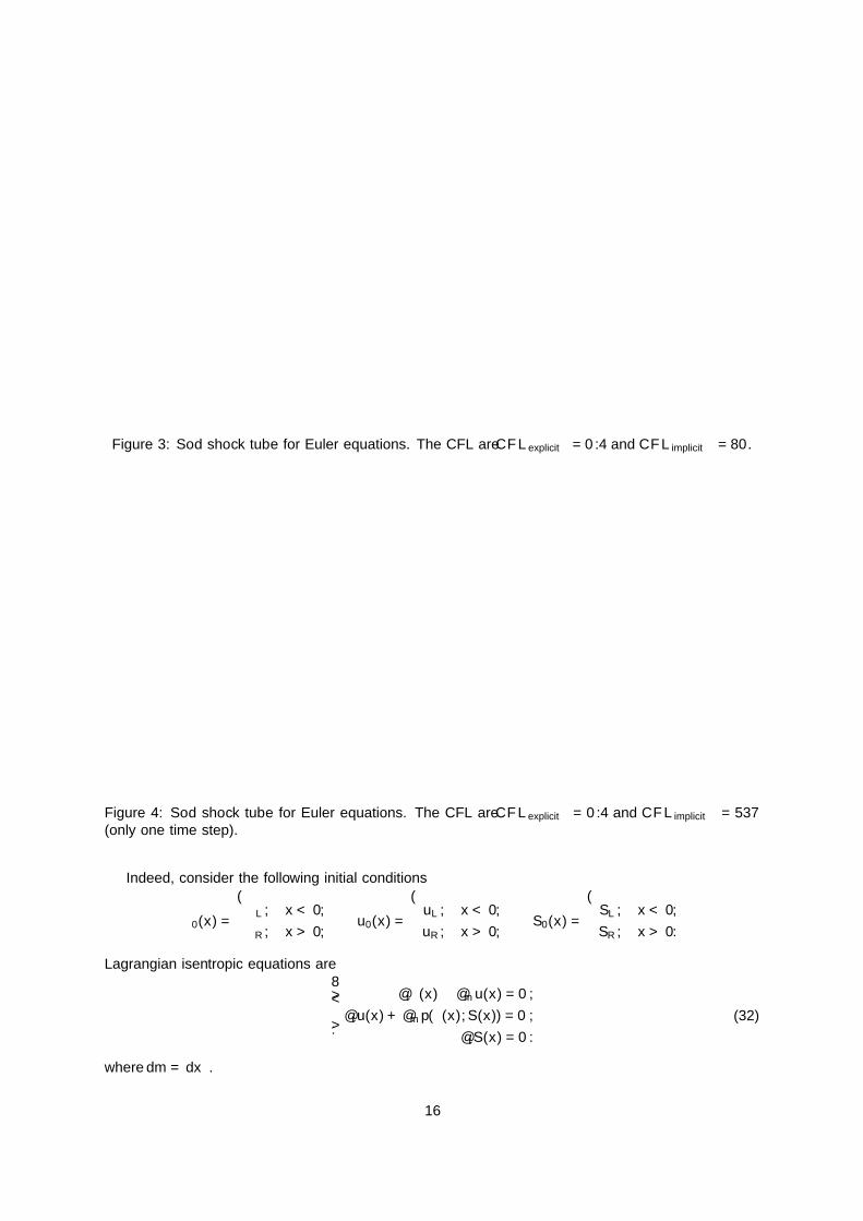
waves as well as the shock. On the contrary, the contact discontinuity is still at the correct location.As it can be seen in Figure 3, one observes that when the CFL tends to be very large, there is more
numerical dissipation on shocks and rarefaction waves but the contact discontinuity still seems to be atthe right position.
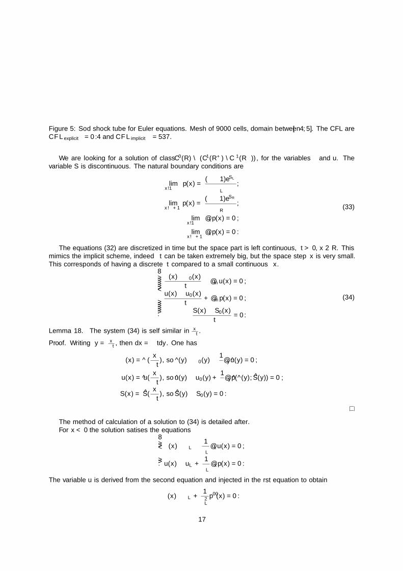
The solution of Figure 4 shows the unconditional stability of the implicit scheme.
14

0.1
0.2
0.3
0.4
0.5
0.6
0.7
0.8
0.9
1
0 0.2 0.4 0.6 0.8 1
Pressure
ImplicitExplicit
0.1
0.2
0.3
0.4
0.5
0.6
0.7
0.8
0.9
1
0 0.2 0.4 0.6 0.8 1
Density
ImplicitExplicit
0
0.1
0.2
0.3
0.4
0.5
0.6
0.7
0.8
0.9
1
0 0.2 0.4 0.6 0.8 1
Velocity
ImplicitExplicit
4.5
5
5.5
6
6.5
7
7.5
8
8.5
9
0 0.2 0.4 0.6 0.8 1
Entropy
ImplicitExplicit
Figure 1: Sod shock tube for Euler equations. The CFL are CFLexplicit = 0.4 and CFLimplicit = 0.4.
0.1
0.2
0.3
0.4
0.5
0.6
0.7
0.8
0.9
1
0 0.2 0.4 0.6 0.8 1
Pressure
ImplicitExplicit
0.1
0.2
0.3
0.4
0.5
0.6
0.7
0.8
0.9
1
0 0.2 0.4 0.6 0.8 1
Density
ImplicitExplicit
0
0.1
0.2
0.3
0.4
0.5
0.6
0.7
0.8
0.9
1
0 0.2 0.4 0.6 0.8 1
Velocity
ImplicitExplicit
4.5
5
5.5
6
6.5
7
7.5
8
8.5
9
0 0.2 0.4 0.6 0.8 1
Entropy
ImplicitExplicit
Figure 2: Sod shock tube for Euler equations. The CFL are CFLexplicit = 0.4 and CFLimplicit = 40.
A remark can be done on the position of the contact discontinuity that is slightly shifted. To explainthe origin of this misplacement, we can evoke the fact that the interaction with the boundaries of thedomain is very important. To validate this hypothesis, we performed another calculation (same initialconditions and final time) on a domain 9 times larger. The results are visible in Figure 5, and the contactdiscontinuity is once again well positioned.
6.2 Position of the contact discontinuityWe develop hereafter a possible explanation for the precision of the position for the contact discontinuityin Figure 5. It deals with the integration of the Riemann problem.
15
0.1
0.2
0.3
0.4
0.5
0.6
0.7
0.8
0.9
1
0 0.2 0.4 0.6 0.8 1
Pressure
ImplicitExplicit
0.1
0.2
0.3
0.4
0.5
0.6
0.7
0.8
0.9
1
0 0.2 0.4 0.6 0.8 1
Density
ImplicitExplicit
0
0.1
0.2
0.3
0.4
0.5
0.6
0.7
0.8
0.9
1
0 0.2 0.4 0.6 0.8 1
Velocity
ImplicitExplicit
4.5
5
5.5
6
6.5
7
7.5
8
8.5
9
0 0.2 0.4 0.6 0.8 1
Entropy
ImplicitExplicit
Figure 3: Sod shock tube for Euler equations. The CFL are CFLexplicit = 0.4 and CFLimplicit = 80.
0.1
0.2
0.3
0.4
0.5
0.6
0.7
0.8
0.9
1
0 0.2 0.4 0.6 0.8 1
Pressure
ImplicitExplicit
0.1
0.2
0.3
0.4
0.5
0.6
0.7
0.8
0.9
1
0 0.2 0.4 0.6 0.8 1
Density
ImplicitExplicit
0
0.1
0.2
0.3
0.4
0.5
0.6
0.7
0.8
0.9
1
0 0.2 0.4 0.6 0.8 1
Velocity
ImplicitExplicit
4.5
5
5.5
6
6.5
7
7.5
8
8.5
9
0 0.2 0.4 0.6 0.8 1
Entropy
ImplicitExplicit
Figure 4: Sod shock tube for Euler equations. The CFL are CFLexplicit = 0.4 and CFLimplicit = 537(only one time step).
Indeed, consider the following initial conditions
τ0(x) =
τL, x < 0,
τR, x > 0,u0(x) =
uL, x < 0,
uR, x > 0,S0(x) =
SL, x < 0,
SR, x > 0.
Lagrangian isentropic equations are∂tτ(x)− ∂mu(x) = 0,
∂tu(x) + ∂mp(τ(x), S(x)) = 0,
∂tS(x) = 0.
(32)
where dm = ρdx.
16
0.1
0.2
0.3
0.4
0.5
0.6
0.7
0.8
0.9
1
0 0.2 0.4 0.6 0.8 1
Density
ImplicitExplicit
Figure 5: Sod shock tube for Euler equations. Mesh of 9000 cells, domain between [−4, 5]. The CFL areCFLexplicit = 0.4 and CFLimplicit = 537.
We are looking for a solution of class C0(R) ∩ (C1(R+) ∩ C1(R−)), for the variables τ and u. Thevariable S is discontinuous. The natural boundary conditions are
limx→−∞
p(x) =(γ − 1)eSL
τγL,
limx→+∞
p(x) =(γ − 1)eSR
τγR,
limx→−∞
∂xp(x) = 0,
limx→+∞
∂xp(x) = 0.
(33)
The equations (32) are discretized in time but the space part is left continuous, ∆t > 0, x ∈ R. Thismimics the implicit scheme, indeed ∆t can be taken extremely big, but the space step ∆x is very small.This corresponds of having a discrete ∆t compared to a small continuous ∆x.
τ(x)− τ0(x)
∆t− ∂mu(x) = 0,
u(x)− u0(x)
∆t+ ∂mp(x) = 0,
S(x)− S0(x)
∆t= 0.
(34)
Lemma 18. The system (34) is self similar in x∆t .
Proof. Writing y = x∆t , then dx = ∆tdy. One has
τ(x) = τ(x
∆t), so τ(y)− τ0(y)− 1
ρ∂yu(y) = 0,
u(x) = u(x
∆t), so u(y)− u0(y) +
1
ρ∂yp(τ(y), S(y)) = 0,
S(x) = S(x
∆t), so S(y)− S0(y) = 0.
The method of calculation of a solution to (34) is detailed after.For x < 0 the solution satisfies the equations
τ(x)− τL −1
ρL∂xu(x) = 0,
u(x)− uL +1
ρL∂xp(x) = 0.
The variable u is derived from the second equation and injected in the first equation to obtain
τ(x)− τL +1
ρ2L
p′′(x) = 0.
17
Introducing the enthalpy H(p, S) = e+ pτ , one has dH = de+ pdτ + τdp = TdS + τdp, hence
∂H
∂p(p, SL)− τL +
1
ρL2p′′(x) = 0.
Factorizing, one gets1
ρL2p′′(x) +
∂
∂p(H(p, SL)− pτL) = 0.
One obtains∂
∂x
(1
ρL2
(p′(x))2
2+H(p, SL)− pτL
)= 0.
Therefore1
ρL2
(p′(x))2
2+H(p, SL)− pτL = KL.
Using the boundary conditions (33), the integration constant is KL = eL.
1
ρL2
(p′(x))2
2+H(p, SL)− pτL − eL = 0.
Sop′(x)
2
2ρL2= −H(p, SL) + pτL + eL.
One finally obtainsp′(x) = ±ρL
√−2H(p, SL) + 2pτL + 2eL. (35)
For x > 0, the solution verifies the equationsτ(x)− τR −
1
ρR∂xu(x) = 0,
u(x)− uR +1
ρR∂xp(x) = 0.
We apply the same method than in the case x < 0, and check that the solution is of the same kind. Onefinally finds an expression for p′
p′(x) = ±ρR√−2H(p, SR) + pτR + eR. (36)
At the interface, when x = 0, the continuity conditions are
p(0−) = p(0+) = p?, u(0−) = u(0+) = u?,
with p? ∈ R. One gets
u? = uL −1
ρLp′(0−) = uR −
1
ρRp′(0+).
That is−uL +
1
ρLp′(0−) = −uR +
1
ρRp′(0+).
Using (35) and (36), one finds the scalar equation
−uL ±√−2H(p?, SL) + 2p?τL + 2eL = −uR ±
√−2H(p?, SR) + 2p?τR + 2eR
where p? is the unknown.In the numerical examples, we took initial conditions of a Sod shock tube, that are recalled hereafter.
uL = uR = 0, ρL =1
τL= 1, ρR =
1
τR=
1
8, pL = 1, pR = 0.1, γ = 1, 4,
eSL =10
4, eSR =
81.4
4.
18
As uL = uR = 0, one has
−H(p?, SL) + p?τL + eL = −H(p?, SR) + p?τR + eR. (37)
Using the perfect gas law, one can rewrite the equation in terms of p and S.
τ =((γ − 1)eS)
1γ
p1γ
, e =pτ
γ − 1= (γ − 1)
1γ−1e
Sγ p1− 1
γ .
One obtains
eSLγ
− γ
γ − 1p?1− 1
γ + p− 1γ
L p? +p
1− 1γ
L
γ − 1
= eSRγ
− γ
γ − 1p?1− 1
γ + p− 1γ
R p? +p
1− 1γ
R
γ − 1
.Lemma 19. The equation (37) admits a unique positive solution p? ∈ [pR, pL].
Proof. Let us denote fL(p) = −H(p, SL) + pτL + eL, and fR(p) = −H(p, SR) + pτR + eR, so that (37) isrewritten as fL(p?)− fR(p?) = 0.
The properties of the function fL are the following. One has fL(pL) = 0, f ′L(pL) = −∂H(pL,SL)∂p +τL =
−τL + τL = 0, and f ′′L(p) = −∂2H(p,S)∂p2 = −∂τ∂p = 1
ρ2c2 > 0. With the same calculations, one findsfR(pR) = 0, f ′R(pR) = 0 and f ′′R(p) > 0. The two functions fL and fR are strictly convex, with aminimum value equal to 0, obtained respectively for pL and pR.
Let us denote f(p) = fL(p) − fR(p). One analyzes the function f in the case of the Sod shocktube, that is for pR 6 p 6 pL. One obtains f(pR) = fL(pR) > 0, and f(pL) = −fR(pL) < 0. Thefunction f changes sign, so it takes at least once the value 0 in between pR and pL, which validates theexistence of a solution. To have the uniqueness, one needs to prove the monotonicity of f . One hasf ′(p) = f ′L(p) − f ′R(p). For all pR < p < pL, one finds f ′L(p) < 0 and f ′R(p) > 0, so f ′(p) < 0 whichconcludes to the monotonicity of f , and the uniqueness of the solution to (37).
Numerically, we calculated with a Newton method that the solution to (37) is approximately equal top? = 0.2559. It corresponds to a velocity of u? = 0.8789. The exact value of the velocity for the Riemannproblem at the contact discontinuity is uexact = 0.9275. This value is found in Toro,32 [Table 4.3, p 131].The difference between u? and uexact is equal to 5.2%, which is a satisfying accuracy considering thatthe implicit simulation performs with only one time step. In our mind, this small relative error of 5.2%is the reason why the contact discontinuity of the implicit solver is approximately superimposed with thereference one in Figure 5.We observed a similar behavior for all the other test problems and we believeit is a strong asset of this family of implicit Lagrangian schemes.
7 Conclusion
We have used a strategy of predictor-corrector scheme, based on the previous work4 in Eulerian coordi-nates, to solve numerically the Euler equations. We have defined an abstract frame in order to analyzea family of implicit schemes written under the peculiar form (8). We have proved the existence anduniqueness of a solution to the prediction step of our implicit scheme. We provided two examples usingthis result and led numerical tests that have indeed corroborated the theoretical statements of stability.The second example is in the Appendix. The numerical illustrations compared the implicit scheme toan explicit scheme of reference, and showed the precision of this new algorithm in these cases.
In a future work, it would be interesting to generalize this method to the case of thin elasto-plasticstructures using Kluth and Després21 or Maire et al.23 We could also try to improve this work by usinga more elaborate flux such as a two state solver flux, or increase the scheme order at the order 2. It willprobably ameliorate the precision, but it stays to evaluate the cost of simulation that it would generate.The multi-dimensional version would need a more advanced management for the displacement of themesh, but the principal ingredients of Theorem 4 should remain similar.
Other numerical examples that are more realistic have to be performed to evaluate the pertinance ofthis algorithm. Theoretically as well, it would be great to have an explanation on the rapid convergence ofthe Newton algorithm for the prediction step, and to have a more elegant proof of the entropy inequalitiesusing the frame (8).
19
A Traffic flow problem
A.1 Formulation under the form (8)As another application of Theorem 4, consider the traffic flow problem in Lagrangian formalism
∂tτ + ∂mf(τ) = 0, f(τ) = −u(τ) = τ−1 − 1, (38)
where ρ = 1τ > 0 is the density, f is the flux and u is the velocity. The mass variable is dm = ρ0(x)dx.
After discretizing this problem in time and space on a meshM composed of N > 0 cells denoted by j,the following implicit scheme is obtained
τn+1j − τnj
∆t+
1τn+1j+1
− 1τn+1j
∆m= 0,
which can be rewritten as
τn+1j − τnj +
∆t
∆m
(1
τn+1j+1
− 1
τn+1j
)= 0. (39)
This scheme is provided with periodic boundary conditions. This problem only needs one step to besolved implicitly, the unconditional stability of (39) will be proved further on.
Let us suppose that τj is positive for all j ∈ 1, . . . , N and let us denote ν = ∆t∆m . In the rest of
this Section one uses the fact that ρn+1j = 1
τn+1j
and the dependence in time is omitted for the sake of
simplicity. The scheme becomes1
ρj− 1
ρnj+ ν(ρj+1 − ρj) = 0.
After reorganization, one gets
− 1
ρj+
1
ρnj+ν
2(−ρj−1 + 2ρj − ρj+1) =
ν
2(ρj+1 − ρj−1). (40)
One can now express the implicit scheme under the form (8). The vector of unknowns is defined by
U = (ρj)16j6N . (41)
The matrix of coefficients for the right handside of the equations (40) reads
A =ν
2
0 1 0 · · · 0 −1−1 0 1 0 · · · 0
0. . . . . . . . . . . .
......
. . . . . . . . . . . . 00 · · · 0 −1 0 11 0 · · · 0 −1 0
. (42)
The terms −1 on the first row and 1 on the last row are due to the periodic boundary conditions. Thefunctional J : D → R, is defined on the domain
D = U such that ∀j ∈ 1, . . . , N, ρj > 0. (43)
J is evaluated as follows
J(U) =
N∑j=1
(− log(ρj) +
ρjρnj
)+
N∑j=1
ν
4(ρj − ρj+1)
2. (44)
By construction the jth partial derivative of J , is
∂J
∂ρj= − 1
ρj+
1
ρnj+ν
2(−ρj−1 + ρj + ρj − ρj+1),
which is exactly the left handside of (40).
20
A.2 Application of Theorem 4 for the traffic flowThe function J defined by (44) satisfies Hypothesis 2, and the matrix A given by (42) verifies Hypothesis 3.
Proposition 20. The implicit scheme (39) for the traffic flow has a unique solution.
Proof. Let m = 0, n = N , U = (ρj)j∈1,...,N, A and J defined as in (42) and (44). All the hypothesis ofTheorem 4 are satisfied, so the existence and uniqueness of a solution to the implicit traffic flow scheme(39) is deduced.
A.3 Numerical illustrations
The precision of the implicit scheme is illustrated, compared to the explicit one, see,11 [Chapter 2],both with Upwind fluxes. The aim of this example is to show the well posedness of the scheme andits robustness. In this case, this is now contact discontinuity, rarefaction fan and shocks for which theaccuracy is depicted for large time step.
Explicit scheme:τn+1j − τnj
∆t+
1τnj+1− 1
τnj
∆m= 0,
Implicit scheme:τn+1j − τnj
∆t+
1τn+1j+1
− 1τn+1j
∆m= 0.
The example is performed on a mesh of 100 cells, for a final time t = 1.2 and velocity boundary conditions.The first experiment has the following initial conditions
τ0(x) =
2, x < 0.3,
1.4, 0.3 6 x < 0.7,
1.1, 0.7 6 x.
The boundary condition is uright = 0.5.
0.5
0.55
0.6
0.65
0.7
0.75
0.8
0.85
0.9
0.95
0 0.1 0.2 0.3 0.4 0.5 0.6 0.7 0.8 0.9 1
Density
ImplicitExplicit
0.5
0.55
0.6
0.65
0.7
0.75
0.8
0.85
0.9
0.95
0.2 0.4 0.6 0.8 1 1.2 1.4
Density
ImplicitExplicit
0.5
0.55
0.6
0.65
0.7
0.75
0.8
0.85
0.9
0.95
0.1 0.2 0.3 0.4 0.5 0.6 0.7 0.8 0.9 1 1.1 1.2
Density
ImplicitExplicit
0.5
0.55
0.6
0.65
0.7
0.75
0.8
0.2 0.4 0.6 0.8 1 1.2 1.4 1.6
Density
ImplicitExplicit
Figure 6: Traffic flow problem at different time steps, on a mesh of 100 cells: t = 0, t = 0.25, t = 0.5and t = 1.2. CFLexplicit = 0.4 and CFLimplicit = 40.
One clearly sees in Figure 6 that the implicit scheme is numerically more dissipated than the explicitscheme, both on the rarefaction waves and the shocks. It is explained by the larger CFL, but the resultsare nonetheless similar.
21
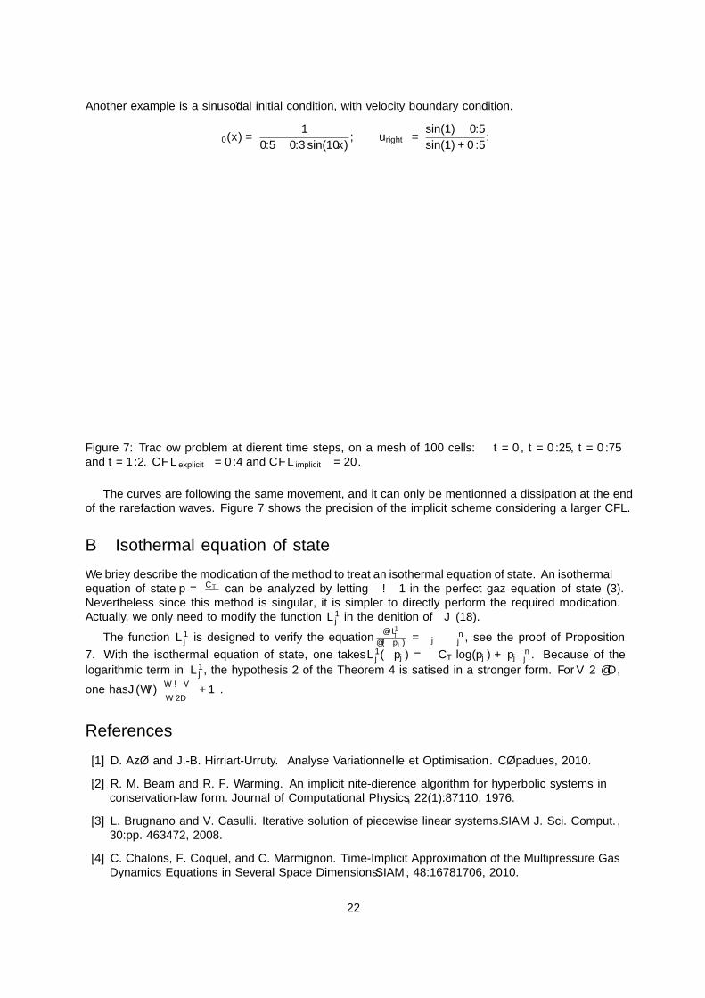
Another example is a sinusoïdal initial condition, with velocity boundary condition.
τ0(x) =1
0.5− 0.3 sin(10x), uright =
sin(1)− 0.5
sin(1) + 0.5.
0.2
0.3
0.4
0.5
0.6
0.7
0.8
0 0.1 0.2 0.3 0.4 0.5 0.6 0.7 0.8 0.9 1
Density
ImplicitExplicit
0.35
0.4
0.45
0.5
0.55
0.6
0.65
0.7
0.75
0.4 0.5 0.6 0.7 0.8 0.9 1 1.1 1.2
Density
ImplicitExplicit
0.2
0.3
0.4
0.5
0.6
0.7
0.8
0.1 0.2 0.3 0.4 0.5 0.6 0.7 0.8 0.9 1 1.1
Density
ImplicitExplicit
0.4
0.45
0.5
0.55
0.6
0.65
0.7
0.75
0.6 0.7 0.8 0.9 1 1.1 1.2 1.3 1.4
Density
ImplicitExplicit
Figure 7: Traffic flow problem at different time steps, on a mesh of 100 cells: t = 0, t = 0.25, t = 0.75and t = 1.2. CFLexplicit = 0.4 and CFLimplicit = 20.
The curves are following the same movement, and it can only be mentionned a dissipation at the endof the rarefaction waves. Figure 7 shows the precision of the implicit scheme considering a larger CFL.
B Isothermal equation of state
We briefly describe the modification of the method to treat an isothermal equation of state. An isothermalequation of state p = CT
τ can be analyzed by letting γ → 1 in the perfect gaz equation of state (3).Nevertheless since this method is singular, it is simpler to directly perform the required modification.Actually, we only need to modify the function L1
j in the definition of J (18).
The function L1j is designed to verify the equation ∂L1
j
∂(−pj) = τj − τnj , see the proof of Proposition7. With the isothermal equation of state, one takes L1
j (−pj) = −CT log(pj) + pjτnj . Because of the
logarithmic term in L1j , the hypothesis 2 of the Theorem 4 is satisfied in a stronger form. For V ∈ ∂D,
one has J(W )W→V−−−−→W∈D
+∞.
References
[1] D. Azé and J.-B. Hirriart-Urruty. Analyse Variationnelle et Optimisation. Cépadues, 2010.
[2] R. M. Beam and R. F. Warming. An implicit finite-difference algorithm for hyperbolic systems inconservation-law form. Journal of Computational Physics, 22(1):87–110, 1976.
[3] L. Brugnano and V. Casulli. Iterative solution of piecewise linear systems. SIAM J. Sci. Comput.,30:pp. 463–472, 2008.
[4] C. Chalons, F. Coquel, and C. Marmignon. Time-Implicit Approximation of the Multipressure GasDynamics Equations in Several Space Dimensions. SIAM, 48:1678–1706, 2010.
22
[5] E. Coddington and N. Levinson. Theory of Ordinary Differential Equations. Tata McGraw-HillEducation, 1955.
[6] F. Coulette, E. Franck, P. Helluyn, A. Ratnani, and E. Sonnendrücker. Implicit time schemes forcompressible fluid models based on relaxation methods. Computers and Fluids, 188:70–85, 2019.
[7] B. Dacorogna. Direct Methods in the Calculus of Variations. Applied Mathematical Sciences,78.Springer-Verlag, Berlin, 1989.
[8] J.-P. Demailly. Analyse Numérique et Equations Différentielles-4ème Ed. EDP sciences, 2016.
[9] I. Demirdzic, Z. Lilek, and Peric M. A collocated finite volume method for predicting flows at allspeeds. Journal for Numerical Methods in Fluids, 16:1029 – 1050, 1993.
[10] B. Després. Weak consistency of the cell-centered Lagrangian GLACE scheme on general meshesin any dimension. Computer Methods in Applied Mechanics and Engineering, 199(41):2669–2679,2010.
[11] B. Després. Numerical Methods for Eulerian and Lagrangian Conservation Laws. Birkhäuser Basel,2017.
[12] A. Ern and J.-L. Guermond. Éléments Finis: Théorie, Applications, Mise en Oeuvre, volume 36.Springer Science & Business Media, 2002.
[13] R. Eymard, T. Gallouët, and R. Herbin. Handbook of Numerical Analysis - Finite Volume Methods,volume 7. Elsevier, 2000.
[14] B. A. Fryxell, P. R. Woodward, P. Colella, and K.-H. Winkler. An implicit-explicit hybrid methodfor lagrangian hydrodynamics. Journal of Computational Physics, 63:283–310, 1986.
[15] T. Gallouët, L. Gastaldo, R. Herbin, and J.-C. Latché. An unconditionally stable pressure correctionscheme for the compressible barotropic Navier-Stokes equations. ESAIM: M2AN, 42:303–331, 2008.
[16] S. K. Godunov. Difference methods of solving equations of gas dynamics. Izd-vo Novosibirsk, un-ta,1962.
[17] J.-B. Hirriart-Urruty. Optimisation et Analyse Convexe. EDP Sciences, 1998.
[18] J.-B. Hirriart-Urruty and C. Lemaréchal. Convex Analysis and Minimization. Springer-Verlag, 1996.
[19] J.-B. Hirriart-Urruty and C. Lemaréchal. Fundamentals of Convex Analysis. Springer-Verlag, 2004.
[20] R. I. Issa. Solution of the implicitly discretised fluid flow equations by operator-splitting. Journalof Computational Physics, 62:40–65, 1985.
[21] G. Kluth and B. Després. Discretization of hyperelasticity on unstructured mesh with a cell-centeredLagrangian scheme. Journal of Computational Physics, 229(24):9092–9118, 2010.
[22] R. J. LeVeque. Finite Volume Methods for Hyperbolic Problems, volume 31. Cambridge universitypress, 2002.
[23] P-H. Maire, R. Abgrall, J. Breil, R. Loubère, and B. Rebourcet. A nominally sceond-order cell-centered Lagrangian scheme for simulating elastic-plastic flows on two-dimensional unstructuredgrids. Journal Of Computational Physics, 235:626–665, 2013.
[24] F. Moukalled and Darwish M. A high-resolution pressure-based algorithm for fluid flow at all speeds.Journal of Computational Physics, 168:101–130, 2001.
[25] W. A. Mulder and B. Van Leer. Experiments with implicit upwind methods for the Euler equations.Journal of Computational Physics, 59:232 – 246, 1985.
[26] G. Patnaik, R. H. Guirguis, J. P. Boris, and Oran E. S. A barely implicit correction for flux-correctedtransport. Journal of Computational Physics, 71:1–20, 1987.
23
[27] S. Peluchon, G. Gallice, and L. Mieussens. A robust implicit-explicit acoustic-transport splittingscheme for two-phase flows. Journal of Computational Physics, 339:328–355, 2017.
[28] E. S. Politis and Giannakoglou K. C. A pressure-based algorithm for high speed turbomachineryflows. Journal for Numerical Methods in Fluids, 25:63–80, 1997.
[29] P.-A. Raviart and E. Godlewski. Numerical Approximation of Hyperbolic Systems of ConservationLaws. Springer, 1996.
[30] N. Seguin, F. Coquel, and E. Godlewski. Approximation par relaxation de systèmes hyperboliques.Séminaire d’analyse appliquée, Université Paris 13, 2008.
[31] D. Serre. Systems of Conservation Laws 1: Hyperbolicity, Entropies, Shock Waves. CambridgeUniversity Press, 1999.
[32] E. F. Toro. Riemann Solvers and Numeriacal Methods for Fluid Dynamics. Springer Verlag, 1999.
[33] G. Toth, R. Keppens, and M. A. Bochev. Implicit and semi-implicit schemes in the versatile advectiocode: Numerical tests. Astronomy and Astrophysics, 332:1159 – 1170, 1998.
[34] D. R. Van der Heuk, C. Vuik, and P. Wesseling. Stability analysis of segregated solution methodsfor compressible flows. Applied Numerical Mathematics, 38:257 – 274, 2001.
[35] D. R. Van der Heuk, C. Vuik, and P. Wesseling. A conservative pressure-correction method for flowat all speed. Computers and Fluids, 32:1113 – 1132, 2003.
[36] D. Vidovic, A. Segal, and P. Wesseling. A superlinearly convergent Mach-uniform finite volumemethod for Euler equations on staggered unstructured grids. Journal of Computational Physics,217:277–294, 2006.
24