implicit collusion through portfolio diversification

A NEW LOOK AT OLIGOPOLY: IMPLICIT COLLUSION

THROUGH PORTFOLIO DIVERSIFICATION

JOSE AZAR

A DISSERTATION

PRESENTED TO THE FACULTY

OF PRINCETON UNIVERSITY

IN CANDIDACY FOR THE DEGREE

OF DOCTOR OF PHILOSOPHY

RECOMMENDED FOR ACCEPTANCE

BY THE DEPARTMENT OF

ECONOMICS

ADVISER: CHRISTOPHER A. SIMS

MAY 2012

c© Copyright by Jose Azar, 2012.

All rights reserved.

Abstract

My dissertation is a theoretical and empirical study of the effects of portfolio diver-

sification on oligopolistic industries. The first chapter serves as the introduction,

and explains how the prominent role of institutional investors in US stock mar-

kets, who tend to own more diversified portfolios than individual households, has

increased the relevance of portfolio diversification on market structure.

In the second chapter I develop a model of oligopoly with shareholder voting.

Instead of assuming that firms maximize profits, the objective of the firms is de-

cided by majority voting. This implies that portfolio diversification generates tacit

collusion. In the limit, when all shareholders are completely diversified, the firms

act as if they were owned by a single monopolist.

The third chapter introduces the model in a general equilibrium context. In

a model of general equilibrium oligopoly with shareholder voting, higher levels

of wealth inequality and/or foreign ownership lead to higher markups and less

efficiency.

In the fourth chapter, I study the evolution of shareholder networks for all pub-

licly traded firms in the United States between 2000 and 2011. The most important

conclusion of the analysis is that the density of the network has more than doubled

over the period, and this is robust to the threshold level chosen.

In the fifth chapter, I study the empirical relationship between common own-

ership and interlocking directorships. Firm pairs with higher levels of common

ownership are more likely to share directors, and their distance in the network of

directors is smaller on average. The evidence presented in this chapter suggests

that institutional investors play an active role in corporate governance. In particu-

lar, it supports the hypothesis that institutional shareholders have influence on the

board of directors.

iii

In the sixth chapter, I study empirically the relationship between networks of

common ownership and market power. Industries with higher levels of common

ownership have higher markups on average.

The last chapter concludes with a discussion of policy implications and poten-

tial directions for further research. Based on the theory, I propose a new Herfindahl

index adjusted for portfolio diversification.

iv

Acknowledgements

First and foremost, I am deeply grateful to my advisor, Christopher Sims, for his

invaluable guidance and support througought my PhD journey. I thank Stephen

Morris and Hyun Shin for their advice on my dissertation. I am also grateful to

Dilip Abreu, Avidit Acharya, Roland Benabou, Harrison Hong, Oleg Itskhoki,

Jean-Francois Kagy, Scott Kostyshak, Juan Ortner, Kristopher Ramsay, Doron

Ravid, Jose Scheinkman, David Sraer, Wei Xiong, and seminar participants at

Princeton University for helpful comments. I also thank Bobray Bordelon at the

Economic Library, and Laura Hedden, Elizabeth Smolinksi, Robin Hauer, and

Karen Neukirchen for their generous help throughout the job market.

This work was partially supported by the Center for Science of Information

(CSoI), an NSF Science and Technology Center, under grant agreement CCF-

0939370.

v

To my parents, Sara and Hector.

vi

Contents

Abstract . . . . . . . . . . . . . . . . . . . . . . . . . . . . . . . . . . . . . . . iii

Acknowledgements . . . . . . . . . . . . . . . . . . . . . . . . . . . . . . . . v

List of Tables . . . . . . . . . . . . . . . . . . . . . . . . . . . . . . . . . . . . x

List of Figures . . . . . . . . . . . . . . . . . . . . . . . . . . . . . . . . . . . xii

1 Introduction 1

2 Oligopoly with Shareholder Voting 5

2.1 Introduction . . . . . . . . . . . . . . . . . . . . . . . . . . . . . . . . . 5

2.2 Literature Review . . . . . . . . . . . . . . . . . . . . . . . . . . . . . . 8

2.3 The Basic Model: Oligopoly with Shareholder Voting . . . . . . . . . 11

2.4 The Case of Complete Diversification . . . . . . . . . . . . . . . . . . 15

2.5 An Example: Quantity and Price Competition . . . . . . . . . . . . . 20

2.5.1 Homogeneous Goods . . . . . . . . . . . . . . . . . . . . . . . 20

2.5.2 Differentiated Goods . . . . . . . . . . . . . . . . . . . . . . . . 26

2.6 Summary . . . . . . . . . . . . . . . . . . . . . . . . . . . . . . . . . . . 29

3 Oligopoly with Shareholder Voting in General Equilibrium 33

3.1 Introduction . . . . . . . . . . . . . . . . . . . . . . . . . . . . . . . . . 33

3.2 Literature Review . . . . . . . . . . . . . . . . . . . . . . . . . . . . . . 35

3.3 Model Setup . . . . . . . . . . . . . . . . . . . . . . . . . . . . . . . . . 36

3.4 Voting Equilibrium with Consumption . . . . . . . . . . . . . . . . . . 38

vii

3.5 Endogenous Corporate Social Responsibility, Inequality, and For-

eign Ownership . . . . . . . . . . . . . . . . . . . . . . . . . . . . . . . 42

3.6 Solving for the Equilibrium with Incomplete Diversification . . . . . 43

3.7 Relaxing the Quasilinearity Assumption . . . . . . . . . . . . . . . . . 44

3.8 Summary . . . . . . . . . . . . . . . . . . . . . . . . . . . . . . . . . . . 46

4 The Evolution of Shareholder Networks in the United States: 2000-2011 49

4.1 Introduction . . . . . . . . . . . . . . . . . . . . . . . . . . . . . . . . . 49

4.2 Data Description . . . . . . . . . . . . . . . . . . . . . . . . . . . . . . 51

4.3 The Increase in Shareholder Network Density . . . . . . . . . . . . . . 51

4.4 Increasing Concentration of Ownership Among Institutional Investors 54

4.5 How Long Do Blockholdings Last? . . . . . . . . . . . . . . . . . . . . 55

4.6 Evolution of the Degree Distributions . . . . . . . . . . . . . . . . . . 57

4.7 Density of Subnetworks by Industrial Sector . . . . . . . . . . . . . . 57

4.8 Summary . . . . . . . . . . . . . . . . . . . . . . . . . . . . . . . . . . . 58

5 Common Shareholders and Interlocking Directorships 84

5.1 Introduction . . . . . . . . . . . . . . . . . . . . . . . . . . . . . . . . . 84

5.2 Data Description . . . . . . . . . . . . . . . . . . . . . . . . . . . . . . 85

5.2.1 Weighted Measures of Common Ownership . . . . . . . . . . 87

5.2.2 Firm-Pair Level Variables . . . . . . . . . . . . . . . . . . . . . 91

5.3 A Gravity Equation for Director and Shareholder Interlocks . . . . . 92

5.3.1 Have Director Interlocks Increased? . . . . . . . . . . . . . . . 95

5.4 Common Ownership and Interlocking Directorships . . . . . . . . . . 96

5.5 Summary . . . . . . . . . . . . . . . . . . . . . . . . . . . . . . . . . . . 98

6 Shareholder Networks and Market Power 118

6.1 Introduction . . . . . . . . . . . . . . . . . . . . . . . . . . . . . . . . . 118

6.2 Data . . . . . . . . . . . . . . . . . . . . . . . . . . . . . . . . . . . . . . 119

viii

6.3 Regression Analysis . . . . . . . . . . . . . . . . . . . . . . . . . . . . . 123

6.4 Panel Vector Autoregression Analysis . . . . . . . . . . . . . . . . . . 126

6.5 Summary . . . . . . . . . . . . . . . . . . . . . . . . . . . . . . . . . . . 127

7 Conclusion: Adjusting the Herfindahl Index for Portfolio Diversifica-

tion? 144

7.1 A Herfindahl Index Adjusted for Common Ownership . . . . . . . . 145

7.1.1 An Example . . . . . . . . . . . . . . . . . . . . . . . . . . . . . 147

7.2 A Model-Based Measure of Common Ownership at the Firm-Pair

Level . . . . . . . . . . . . . . . . . . . . . . . . . . . . . . . . . . . . . 148

7.3 Possible Directions for Future Research . . . . . . . . . . . . . . . . . 149

Bibliography 151

ix

List of Tables

4.1 Summary Statistics . . . . . . . . . . . . . . . . . . . . . . . . . . . . . 59

4.2 Top 5 Institutional Investors by Number of Blockholdings (3%

Threshold) . . . . . . . . . . . . . . . . . . . . . . . . . . . . . . . . . . 60


Threshold) . . . . . . . . . . . . . . . . . . . . . . . . . . . . . . . . . . 61


Threshold) . . . . . . . . . . . . . . . . . . . . . . . . . . . . . . . . . . 62


5.2 Summary Statistics for Variables at the Firm-Pair Level . . . . . . . . 101

5.3 Correlation Matrix for Common Ownership Variables . . . . . . . . . 102

5.4 Gravity Equations for Common Directors and Common Sharehold-

ers (Logit) . . . . . . . . . . . . . . . . . . . . . . . . . . . . . . . . . . 103

5.5 Gravity Equations for Log Network Distance and for Weighted Mea-

sures of Common Ownership . . . . . . . . . . . . . . . . . . . . . . . 104

5.6 Gravity Equations for Director Interlocks and Log Network Dis-

tance with Common Shareholder Dummy . . . . . . . . . . . . . . . . 105


tance with Maximin . . . . . . . . . . . . . . . . . . . . . . . . . . . . . 106


tance with Sum of Mins . . . . . . . . . . . . . . . . . . . . . . . . . . 107

x


tance with Inner Product . . . . . . . . . . . . . . . . . . . . . . . . . . 108


6.2 Average Markups and Measures of Common Ownership . . . . . . . 130

6.3 Vector Autoregression Results . . . . . . . . . . . . . . . . . . . . . . . 131

6.4 Vector Autoregression Results . . . . . . . . . . . . . . . . . . . . . . . 132

xi

List of Figures

1.1 Percentage Ownership of Institutional Investors in U.S. Stock Markets 4

2.1 Equilibrium Quantities and Prices for Different Levels of Portfolio

Diversification in a Cournot Oligopoly with Homogeneous Goods . 31

2.2 Equilibrium Prices for Different Levels of Portfolio Diversification

in Cournot and Bertrand Oligopoly with Differentiated Goods . . . . 32

3.1 Equilibrium Prices in the Quasilinear General Equilibrium Model

for Different Levels of Initial Wealth Inequality . . . . . . . . . . . . . 47

3.2 Equilibrium Quantity of the Oligopolistic Good in the Quasilinear

General Equilibrium Model for Different Levels of Wealth Inequal-

ity and Diversification (Lognormal Wealth Distribution) . . . . . . . . 48

4.1 Shareholder Network (Random Sample of 1000 Companies in 2010Q4) 63

4.2 Evolution of the Density of the Network of Interlocking Sharehold-

ings: All Firms . . . . . . . . . . . . . . . . . . . . . . . . . . . . . . . . 64


ings: Largest 3000 Firms . . . . . . . . . . . . . . . . . . . . . . . . . . 65


ings: Largest 500 Firms . . . . . . . . . . . . . . . . . . . . . . . . . . . 66

4.5 Fraction of Firms with At Least one Blockholder: All Firms . . . . . . 67

4.6 Fraction of Firms with At Least one Blockholder: Largest 3000 Firms 68

xii

4.7 Fraction of Firms with At Least one Blockholder: Largest 500 Firms . 69

4.8 Fraction of Connections Generated by the Top 5 Institutional Investors 70

4.9 Fraction of Firms Owned by the Top x Institutional Investors: 3%

Threshold . . . . . . . . . . . . . . . . . . . . . . . . . . . . . . . . . . 71


Threshold . . . . . . . . . . . . . . . . . . . . . . . . . . . . . . . . . . 72


Threshold . . . . . . . . . . . . . . . . . . . . . . . . . . . . . . . . . . 73


Threshold, Largest 3000 Firms . . . . . . . . . . . . . . . . . . . . . . . 74





4.15 Cumulative Distribution Function for the Value of the Portfolios

of Institutional Investors as a Share of Total Market Capitalization:

2000 and 2011 . . . . . . . . . . . . . . . . . . . . . . . . . . . . . . . . 77

4.16 Fraction of Blockholdings Surviving Until Next Quarter . . . . . . . . 78

4.17 Fraction of Blockholdings Surviving Until Next Quarter (Top 5 In-

stitutions) . . . . . . . . . . . . . . . . . . . . . . . . . . . . . . . . . . 79

4.18 Cumulative Distribution Functions for the Degrees of the Share-

holder Network at Different Thresholds: 2000 and 2011 . . . . . . . . 80

4.19 Industry Sub-Network Densities in 2011: 3% Threshold . . . . . . . . 81



5.1 Network of Interlocking Directorships for US Firms: 2010 . . . . . . . 109

xiii

5.2 Degree Distribution for the Network of Interlocking Directors: 2001

and 2010 . . . . . . . . . . . . . . . . . . . . . . . . . . . . . . . . . . . 110

5.3 Cubic Spline Polynomial for the Probability of Common Directors

as a Function of the Log of the Product of Firm Sizes . . . . . . . . . . 111

5.4 Cubic Spline Polynomial for the Probability of Common Sharehold-

ers as a Function of the Log of the Product of Firm Sizes . . . . . . . . 112

5.5 Cubic Spline Polynomial for Network Distance as a Function of the

Log of the Product of Firm Sizes . . . . . . . . . . . . . . . . . . . . . 113

5.6 Cubic Spline Polynomial for Maximin as a Function of the Log of

the Product of Firm Sizes . . . . . . . . . . . . . . . . . . . . . . . . . . 114

5.7 Cubic Spline Polynomial for the Sum of Mins as a Function of the


5.8 Cubic Spline Polynomial for the Inner Product as a Function of the


5.9 Evolution of the Probability of Director Interlocks . . . . . . . . . . . 117

6.1 Shareholder Network Density over Time . . . . . . . . . . . . . . . . 133

6.2 Average and Median Markups over Time . . . . . . . . . . . . . . . . 134

6.3 Average Markup, by Decile of Log Assets . . . . . . . . . . . . . . . . 135

6.4 Average Fraction of Periods with Negative Income (Before Taxes)

and Average Number of Periods with Observations, by Decile of

Log Assets . . . . . . . . . . . . . . . . . . . . . . . . . . . . . . . . . . 136

6.5 Average Markup, by Quintile of Within-Industry Degree . . . . . . . 137

6.6 Average Fraction of Periods with Negative Income, by Quintile of

Within-Industry Degree . . . . . . . . . . . . . . . . . . . . . . . . . . 138

6.7 Average Number of Periods with Observations, by Quintile of

Within-Industry Degree . . . . . . . . . . . . . . . . . . . . . . . . . . 139

xiv

6.8 Response of the Average Industry Markup to Shocks to Ownership

Structure Variables . . . . . . . . . . . . . . . . . . . . . . . . . . . . . 140

6.9 Response of Ownership Structure Variables to Shocks to Average

Industry Markups . . . . . . . . . . . . . . . . . . . . . . . . . . . . . . 141

6.10 Response of the Average Industry Markup to Shocks to Ownership

Structure Variables (including Industry Fixed Effects) . . . . . . . . . 142

6.11 Response of Ownership Structure Variables to Shocks to Average

Industry Markups (including Industry Fixed Effects) . . . . . . . . . 143

xv

Chapter 1

Introduction

What is the effect of ownership structure on market structure? Models of oligopoly

generally abstract from financial structure by assuming that each firm in an indus-

try is owned by a separate agent, whose objective is to maximize the profits of the

firm. In these models, any given firm is in direct competition with all the other

firms in the industry. In practice, however, ownership of publicly traded compa-

nies is dispersed among many shareholders. The shareholders of a firm, in turn,

usually hold diversified portfolios, which often contain shares in most of the large

players in an industry. This diversification is, of course, what portfolio theory rec-

ommends that fund managers should do in order to reduce their exposure to risk.

The increasing importance in equity markets of institutional investors, which tend

to hold more diversified portfolios than individual households, suggests that di-

versification has increased through the second half of the twentieth century and

the beginning of the twenty-first. Figure 1.1 shows that the fraction of U.S. corpo-

rate equities owned by institutional investors increased from less than 10 percent

in the early 1950s to more than 60 percent in 2010.1

1See also Gompers and Metrick (2001) and Gillan and Starks (2007).

1

In chapter 2, I develop a model of oligopoly with shareholder voting. The in-

dustrial organization literature usually assumes that the objective of the firm is

to maximize profits. Thus, it abstracts from ownership structure, and in partic-

ular, from other financial interests that the shareholders may have. The finance

literature, on the other hand, usually models firms as either simply a random

return (Markowitz), or perfectly competitive (Arrow-Debreu), and therefore ab-

stracts from the effect that portfolio decisions may have on market structure. In

the theory that I develop, firms are non-atomistic and owned by shareholders with

portfolios that may have stakes in several firms. The objective of the firm is de-

rived endogenously through shareholder voting, and therefore the objective will

not be independent profit maximization unless firms are separately owned. In this

model, portfolio diversification generates tacit collusion.

In chapter 3, I develop a model of general equilibrium oligopoly with share-

holder voting. In general equilibrium, firms will also take into account nonprofit

objectives of their shareholders. Thus, they will endogenously engage in corporate

social responsibility. The level of corporate social responsibility in equilibrium de-

pends on the level of wealth inequality, with more inequality generating less cor-

porate social responsibility and less efficiency.

In chapter 4, I study the evolution of the network of interlocking shareholdings

for the United States between 2000 and 2011. A connection is defined as a pair

of firms having a common institutional shareholder with more than a threshold

percentage ownership in both firms. The density of this network has more than

doubled between 2000 and 2011. The reason for this huge increase in density is an

increase in the number of blockholdings held by the largest institutional investors

throughout the period. While most blockholdings do not last more than a few

years, the survival rate for blockholdings of 3% held by the top 5 institutions has

increased substantially in recent years, and the “life expectancy” of these holdings

2

is high. Within-industry network densities are on average higher than the overall

density, reflecting the fact that firms in the same industry are more likely to be

connected.

In chapter 5, I study the relation between the network of interlocking share-

holders and the network of interlocking directors for a large sample of US firms.

Having common shareholders increases the likelihood of having common direc-

tors substantially, as does being in the same industry. Moreover, there is a positive

interaction effect between having common shareholders and being in the same in-

dustry. This suggests that institutional investors are playing a more activist role in

selecting directors in US companies than previously thought.

In chapter 6, I study the relationship between networks of common owner-

ship and markups at the industry level. The main result is that the industry-

level density of shareholder networks is positively associated with average indus-

try markups. A dynamic analysis using Panel Vector Autoregressions shows that

industry-level density of shareholder networks is a significant predictor of average

markups, but average markups do not have predictive power for industry-level

density.

In chapter 7, I discuss potential implication for policy, and directions for further

research. Applying the model of oligopoly with shareholder voting to a Cournot

setting, I derive an adjusted Herfindahl index that takes into account common

ownership between firms in an industry. I also propose a possible measure of

common ownership at the firm-pair level based on the theory.

3

0%

10%

20%

30%

40%

50%

60%

70%

1950 1960 1970 1980 1990 2000 2010

Figure 1.1Percentage Ownership of Institutional Investors in U.S. Stock Markets

Source: Federal Reserve Flow of Funds.

4

Chapter 2

Oligopoly with Shareholder Voting

2.1 Introduction

Classical models of oligopoly usually abstract from ownership structure by assum-

ing that firms maximize profits. Thus, they assume that each firm is separately

owned. At the same time, financial economics shows that it is in the individual

interest of investors to hold diversified portfolios. Financial economics usually ab-

stracts from the effect of portfolio diversification on market structure by modeling

firms as a random return, as in the case of Markowitz (1952) and the subsequent

literature. Even when firms are modeled as productive units, they are usually as-

sumed to be price-takers, as in the case of Arrow-Debreu models of competitive

equilibrium. Thus, portfolio diversification in the classical models of financial eco-

nomics cannot influence market structure by assumption.

In this chapter, I study the implications of portfolio diversification for equilib-

rium outcomes in oligopolistic industries. The main contribution is the develop-

ment of a model of oligopoly with shareholder voting. Instead of assuming that

firms maximize profits, I model the objective of the firms as determined by the

outcome of majority voting by their shareholders. When shareholders vote on the

5

policies of one company, they take into account the effects of those policies not

just on that particular company’s profits, but also on the profits of the other com-

panies that they hold stakes in. That is, because the shareholders are the residual

claimants in several firms, they internalize the pecuniary externalities that each of

these firms generates on the others that they own, as was pointed out by Gordon

(1990). This leads to a very different world from the one in which firms compete

with each other by maximizing their profits independently, as in classical Cournot

or Bertrand models of oligopoly. In the classical models, the actions of each firm

generate pecuniary externalities for the other firms, but these are not internalized

because each firm is assumed to have a different owner.

Gordon (1990) and Hansen and Lott (1996) argued that, when shareholders are

completely diversified, and there is no uncertainty, they agree unanimously on the

objective of joint profit maximization. However, in practice shareholders are not

completely diversified, and their portfolios are different from each other. More-

over, company profits can be highly uncertain, and shareholders with different

degrees of risk aversion will disagree about company policies even if they all hold

the same portfolios. The model of oligopoly with shareholder voting developed

in this paper, unlike the previous literature, allows for the characterization of the

equilibrium in cases in which shareholders disagree about the policies of the firms.

Some new applications that are made possible by a model with shareholder

disagreement include (a) the characterization of the equilibrium in the case of com-

plete diversification with uncertainty and risk averse shareholders, (b) compara-

tive statics for different levels of portfolio diversification, (c) the derivation of an

adjusted Herfindahl index that incorporates information about common owner-

ship among the firms in an industry, and (d) a model-based measure of common

ownership for pairs of firms.

6

By modeling shareholders as directly voting on the actions of the firms, and

having managers care only about expected vote share, I abstract in this paper from

the conflict of interest between owners and managers. In practice, shareholders

usually do not have a tight control over the companies that they own. Institutional

owners usually hold large blocks of equity, and the empirical evidence suggests

that they play an active role in corporate governance.1 The results of the paper

should thus be interpreted as showing what the outcome is when shareholders

control the managers. From a theoretical point of view, whether agency problems

would prevent firms from internalizing externalities that they generate on other

portfolio firms depends on the assumptions one makes about managerial prefer-

ences. This would only be the case, to some extent, if the utility of managers is

higher when they do not internalize the externalities than when they do.

The theory developed in this chapter shows that assessing the potential for

market power in an industry by using concentration ratios or the Herfindahl in-

dex can be misleading if one does not, in addition, pay attention to the portfolios

of the main shareholders of each firm in the industry. This applies to both horizon-

tally and vertically related firms. In the model, diversification acts as a partial form

of integration between firms. Antitrust policy usually focuses on mergers and ac-

quisitions, which are all-or-nothing forms of integration. It may be beneficial to

pay more attention to the partial integration that is achieved through portfolio di-

versification.

However, the theory has additional, broader implications for normative analy-

sis. Economists generally consider portfolio diversification, alignment of interest

between managers and owners, and competition to be three desirable objectives.

In the model developed in this paper, it is not possible to fully attain all three.

1See, for example, Agrawal and Mandelker (1990), Bethel et al. (1998), Kaplan and Minton(1994), Kang and Shivdasani (1995), Bertrand and Mullainathan (2001), and Hartzell and Starks(2003).

7

Competition and diversification could be attained if shareholders failed to appro-

priately incentivize the managers of the companies that they own. Competition

and maximization of shareholder value are possible if shareholders are not well

diversified. And diversification and maximization of shareholder value are fully

attainable, but the result is collusive. This trilemma highlights that it is not possible

to separate financial policy from competition policy.

2.2 Literature Review

In addition to Gordon (1990) and Hansen and Lott (1996), the theory developed in

this chapter is related to the work of Reynolds and Snapp (1986), who develop a

model of quantity competition in which firms hold partial interests in each other.

This chapter also relates to the literature on aggregation of shareholder prefer-

ences, going back at least to the impossibility result of Arrow (1950). Although his

1950 paper does not apply the results to aggregation of differing shareholder pref-

erences, this problem was in the background of the research on the impossibility

theorem, as Arrow mentions later (Arrow, 1983, p. 2):

“When in 1946 I began a grandiose and abortive dissertation aimed

at improving on John Hicks’s Value and Capital, one of the obvious needs

for generalization was the theory of the firm. What if it had many own-

ers, instead of the single owner postulated by Hicks? To be sure, it could

be assumed that all were seeking to maximize profits; but suppose they

had different expectations of the future? They would then have dif-

fering preferences over investment projects. I first supposed that they

would decide, as the legal framework would imply, by majority voting.

In economic analysis we usually have many (in fact, infinitely many)

alternative possible plans, so that transitivity quickly became a signif-

8

icant question. It was immediately clear that majority voting did not

necessarily lead to an ordering.”

Milne (1981) explicitly applies Arrow’s result to the shareholders’ preference

aggregation problem. Under complete markets and price-taking firms, the Fisher

separation theorem applies, and thus all shareholders unanimously agree on the

profit maximization objective (see Milne 1974, Milne 1981). With incomplete mar-

kets, however, the preference aggregation problem is non-trivial. The literature on

incomplete markets has thus studied the outcome of equilibria with shareholder

voting. For example, see the work of Diamond (1967), Milne (1981), Dreze (1985),

Duffie and Shafer (1986), DeMarzo (1993), Kelsey and Milne (1996), and Dierker

et al. (2002). This literature keeps the price-taking assumption, so there is no po-

tential for firms exercising market power.

From a modeling point of view, I rely extensively on insights and results from

probabilistic voting theory. For a survey of this literature, see the first chapter of

Coughlin (1992). I have also benefited from the exposition of this theory in Ace-

moglu (2009). These models have been widely used in political economy, but not,

to my knowledge, in models of shareholder elections. I also use insights from the

work on multiple simultaneous elections by Alesina and Rosenthal (1995), Alesina

and Rosenthal (1996), Chari et al. (1997). Ahn and Oliveros (2010) have studied

further under what conditions conditional sincerity is obtained as an outcome of

strategic voting.

This chapter contributes to the literature on the intersection of corporate finance

and industrial organization. The interaction between these two fields has received

surprisingly little attention (see Cestone (1999) for a recent survey). The corporate

finance literature, since the classic book by Berle and Means (1940), has focused

mainly on the conflict of interest between shareholders and managers, rather than

on the effects of ownership structure on product markets, while industrial orga-

9

nization research usually abstracts from issues of ownership to focus on strategic

interactions in product markets. It is worth mentioning the seminal contribution

of Brander and Lewis (1986), who show that the use of leverage can affect the

equilibrium in product markets by inducing oligopolistic firms to behave more ag-

gressively. Fershtman and Judd (1987) study the principal-agent problem faced

by owners of firms in Cournot and Bertrand oligopoly games. Poitevin (1989) ex-

tends the model of Brander and Lewis (1986) to the case where two firms borrow

from the same bank. The bank has an incentive to make firms behave less ag-

gressively in product markets, and can achieve a partially collusive outcome. In a

footnote, Brander and Lewis (1986) mention that, although they do not study them

in their paper, it would be interesting to consider the possibility that the rival firms

are linked through interlocking directorships or through ownership by a common

group of shareholders.

Finally, this paper touches on themes that are present in the literature on the

history of financial regulation and the origins of antitrust. DeLong (1991) studies

the relationship between the financial sector and industry in the U.S. during the

late nineteenth and early twentieth century. He documents that representatives of

J.P. Morgan and other financial firms sat on the boards of several firms within an

industry. He argues that this practice, while helping to align the interests of own-

ership and control, also led to collusive behavior. Roe (1996) and Becht and De-

Long (2005) study the political origins of the US system of corporate governance.

In particular, they focus on the weakness of financial institutions with respect to

management in the US relative to other countries, especially Germany and Japan.

They argue that this weakness was can be understood, at least in part, as the out-

come of a political process. In the US, populist forces and the antitrust movement

achieved their objective of weakening the large financial institutions that in other

countries exert a tighter control over managers.

10

2.3 The Basic Model: Oligopoly with Shareholder

Voting

An oligopolistic industry consists of N firms. Firm n’s profits per share are random

and depend both on its own policies pn and on the policies of the other firms, p−n,

as well as the state of nature ω ∈ Ω:

πn = πn(pn, p−n; ω).

Suppose that pn ∈ Sn ⊆ RK, so that policies can be multidimensional. The policies

of the firm can be prices, quantities, investment decisions, innovation, or in general

any decision variable that the firm needs to choose. In principle, the policies could

be contingent on the state of nature, but this is not necessary.

There is a continuum G of shareholders of measure one. Shareholder g holds

θgn shares in firm n. The total number of shares of each firm is normalized to 1.

Each firm holds its own elections to choose the board of directors, which controls

the firms’ policies. In the elections of company n there is Downsian competition

between two parties, An and Bn. Let ξgJn

denote the probability that shareholder g

votes for party Jn in company n’s elections, where Jn ∈ An, Bn. The expected vote

share of party Jn in firm n’s elections is

ξ Jn =∫

g∈Gθ

gnξ

gJn

dg.

Shareholders get utility from income–which is the sum of profits from all their

shares–and from a random component that depends on what party is in power in

each of the firms. The utility of shareholder g when the policy of firm n is pn, the

11

policies of the other firms are p−n, and the vector of elected parties is JnNn=1 is

Ug(

pn, p−n, JsNs=1

)= Ug(pn, p−n) +

N

∑s=1

σgs (Js),

where Ug(pn, p−n) = E[ug(

∑Ns=1 θ

gs πs(ps, p−s; ω)

)]. The utility function ug of

each group is increasing in income, with non-increasing marginal utility. The

σgn(Jn) terms represent the random utility that shareholder g obtains if party Jn

controls the board of company n. The random utility terms are independent across

firms and shareholders, and independent of the state of nature ω. As a normaliza-

tion, let σgn(An) = 0. I assume that, given p−n, there is an interior pn that maxi-

mizes Ug(pn, p−n).

Let pAn denote the platform of party An and pBn that of party Bn.

Assumption 1. (Conditional Sincerity) Voters are conditionally sincere. That is, in

each firm’s election they vote for the party whose policies maximize their utilities, given the

equilibrium policies in all the other firms. In case of indifference between the two parties, a

voter randomizes.

Conditional sincerity is a natural assumption as a starting point in models of

multiple elections. Alesina and Rosenthal (1996) obtain it as a result of coalition

proof Nash equilibrium in a model of simultaneous presidential and congressional

split-ticket elections. A complete characterization of the conditions under which

conditional sincerity arises as the outcome of strategic voting is an open problem

(for a recent contribution and discussion of the issues, see Ahn and Oliveros 2010).

In this paper, I will treat conditional sincerity as a plausible behavioral assumption,

which, while natural as a starting point, does not necessarily hold in general.

Using Assumption 1, the probability that shareholder g votes for party An is

ξgAn

= P[σ

gn(Bn) < Ug(pAn , p−n)−Ug(pBn , p−n)

].

12

Let us assume that the marginal distribution of σgn,i(Bn) is uniform with support

[−mgn, mg

n]. Denote its cumulative distribution function Hgn . The vote share of party

An is

ξAn =∫

g∈Gθ

gnHg

n [Ug(pAn , p−n)−Ug(pBn , p−n)] dg. (2.1)

Both parties choose their platforms to maximize their expected vote shares.

Assumption 2. (Differentiability and Concavity of Vote Shares) For all firms n =

1, . . . , N, the vote share of party An is differentiable and strictly concave as a function of

pn given the policies of the other firms p−n and the platform of party Bn. The vote share is

continuous as a function of p−n. Analogous conditions hold for the vote share of party Bn.

Elections for all companies are held simultaneously, and the two parties in each

company announce their platforms simultaneously as well. A pure-strategy Nash

equilibrium for the industry is a set of platforms pAn , pBnNn=1 such that, given

the platform of the other party in the firm, and the winning policies in all the

other firms, a party chooses its platform to maximize its vote share. The first-order

condition for party An is

∫g∈G

12mg

nθ

gn

∂Ug(pAn , p−n)

∂pAn

dg = 0, (2.2)

where∂Ug(pn, p−n)

∂pAn

=

(∂Ug(pAn , p−n)

∂p1An

, . . . ,∂Ug(pAn , p−n)

∂pKAn

).

In the latter expression, pkAn

is the kth component of the policy vector pAn . The

derivatives in terms of the profit functions are

∂Ug(pn, p−n)

∂pAn

= E

[(ug)′

(N

∑s=1

θgs πs(ps, p−s; ω)

)N

∑s=1

θgs

∂πs(ps, p−s)

∂pn

].

13

The maximization problem for party Bn is symmetric. Because the individual util-

ity functions have an interior maximum, the problem of maximizing vote shares

given the policies of the other firms will also have an interior solution.

To ensure that an equilibrium in the industry exists, we need an additional

technical assumption.

Assumption 3. The strategy spaces Sn are nonempty compact convex subsets of RK.

Theorem 1. Suppose that Assumptions 1, 2, and 3 hold. Then, a pure-strategy equilib-

rium of the voting game exists. The equilibrium is symmetric in the sense that pAn =

pBn = p∗n for all n. The equilibrium policies solve the system of N×K equations in N×K

unknowns ∫g∈G

12mg

nθ

gn

∂Ug(p∗n, p∗−n)

∂pndg = 0 for n = 1, . . . , N. (2.3)

Proof. Consider the election at firm n, given that the policies of the other firms are

equal to p−n. Given the conditional sincerity assumption, the vote share of party

An is as in equation (2.1), and a similar expression holds for the vote share of party

Bn. As we have already noted, each party’s maximization problem has an interior

solution conditional on p−n. The first-order conditions for each party are the same,

and thus the best responses for both parties are the same. We can think of the

equilibrium at firm n’s election given the policies of the other firms as establishing

a reaction function for the firm, pn(p−n). These reaction functions are nonempty,

upper-hemicontinuous, and convex-valued. Thus, we can apply Kakutani’s fixed

point theorem to show that an equilibrium exists, in a way that is analogous to that

of existence of Nash equilibrium in games with continuous payoffs.

The system of equations in (2.3) corresponds to the solution to the maximiza-

tion of the following utility functions

∫g∈G

χgnθ

gnUg(pn, p−n)dg for n = 1, . . . , N, (2.4)

14

where the nth function is maximized with respect to pn, and where χgn ≡ 1

2mgn.

Thus, the equilibrium for each firm’s election is characterized by the maximization

of a weighted average of the utilities of its shareholders. The weight that each

shareholder gets at each firm depends both on the number of shares held in that

firm, and on the dispersion of the random utility component for that firm. Note

that the weights in the average of shareholder utilities are different at different

firms.

The maximization takes into account the effect of the policies of firm n on the

profits that shareholders get from every firm, not just firm n. Thus, when the

owners of a firm are also the residual claimants for other firms, they internalize

some of the pecuniary externalities that the actions of the first firm generate for the

other firms that they hold.

2.4 The Case of Complete Diversification

We will find it useful to define the following concepts:

Definition 1. (Market Portfolio) A market portfolio is any portfolio that is proportional

to the total number of shares of each firm. Since we have normalized the number of shares

of each firm to one, a market portfolio has the same number of shares in every firm.

Definition 2. (Complete Diversification) We say that a shareholder who holds a market

portfolio is completely diversified.

Definition 3. (Uniformly Activist Shareholders) We say that a shareholder is uniformly

activist if the density of the distribution of σgn(Bn) is the same for every firm n.

Shareholders having a high density of σgn(Bn) have a higher weight in the equi-

librium policies of firm n for a given number of shares. Thus, we can think of

15

shareholders having high density as being more “activist” when it comes to influ-

encing the decisions of that firm. If all shareholders are uniformly activist, then

some shareholders can be more activist than others, but the level of activism for

each shareholder is constant across firms.

Theorem 2. Suppose all shareholders are completely diversified, and shareholders are uni-

formly activist. Then the equilibrium of the voting game yields the same outcome as the

one that a monopolist who owned all the firms and maximized a weighted average of the

utilities of the shareholders would choose.

Proof. Because of complete diversification, a shareholder g holds the same number

of shares θg in each firm. The equilibrium now corresponds to the solution of

maxpn

∫g∈G

χgnθgUg(pn, p−n)dg for n = 1, . . . , N.

With the assumption that shareholders are uniformly activist, χgn is the same for

every firm, and thus the objective function is the same for all n. The problem can

thus be rewritten as

maxpnN

n=1

∫g∈G

χgθgUg(pn, p−n)dg.

This is the problem that a monopolist would solve, if her utility function was a

weighted average of the utilities of the shareholders. The weight of shareholder g

is equal to χgθg.

Note that, although all the shareholders hold proportional portfolios, there is

still a conflict of interest between them. This is due to the fact that there is uncer-

tainty and shareholders, unless they are risk neutral, care about the distribution of

joint profits, not just the expected value. For example, they may have different de-

grees of risk aversion, both because some may be wealthier than others (i.e. hold a

bigger share of the market portfolio), or because their utility functions differ. Thus,

16

although all shareholders are fully internalizing the pecuniary externalities that the

actions of each firm generates on the profits of the other firms, some may want the

firms to take on more risks, and some may want less risky actions. Thus, there is

still a non-trivial preference aggregation problem. In what follows, I will show that

when shareholders are risk neutral, or when there is no uncertainty, then there is

no conflict of interest between shareholders: they all want the firms to implement

the same policies.

We will now show that, when all shareholders are completely diversified and

risk neutral, the solution can be characterized as that of a profit-maximizing mo-

nopolist. In this case, we do not need the condition that χgn is independent of n.

In fact, in this case, there is no conflict of interest between shareholders, since they

uniformly agree on the objective of expected profit maximization. Thus, this result

is likely to hold in much more general environments than the probabilistic voting

model of this paper.

Theorem 3. Suppose all shareholders are completely diversified, and their preferences are

risk neutral. Then the equilibrium of the voting game yields the same outcome as the one

that a monopolist who owned all the firms and maximized their joint expected profits would

choose.

Proof. Let the utility function of shareholder g be ug(y) = ag + bgy. Then the

equilibrium is characterized by the solution of

maxpn

∫g∈G

χgnθg

ag + bgE

[N

∑s=1

θgπs(ps, p−s; ω)

]dg for n = 1, . . . , N,

which can be rewritten as

maxpn

k0,n + k1,nE

[N

∑s=1

πs(ps, p−s; ω)

]for n = 1, . . . , N,

17

with k0,n =∫

g∈G χgnθgagdg and k1,n =

∫g∈G χ

gn(θ

g)2bgdg. Since k1,n is positive, this

is the same as maximizing

E

[N

∑s=1

πs(ps, p−s; ω)

],

which is the expected sum of profits of all the firms in the industry. Since the

objective function is the same for every firm, we can rewrite this as

maxpnN

n=1

E

[N

∑s=1

πs(ps, p−s; ω)

].

The intuition behind this result is simple. When shareholders are completely

diversified, their portfolios are identical, up to a constant of proportionality. With-

out risk neutrality, shareholders cared not just about expected profits, but about

the whole distribution of joint profits. With risk neutrality, however, sharehold-

ers only care about joint expected profits, and thus the conflict of interest between

shareholders disappears. The result is that they unanimously want maximization

of the joint expected profits, and the aggregation problem becomes trivial.

Finally, let us consider the case of no uncertainty. In this case, when sharehold-

ers are completely diversified there is also no conflict of interest between them,

and they unanimously want the maximization of joint profits. This is similar to the

case of risk neutrality. As in that case, because preference are unanimous the result

is likely to hold under much more general conditions.

Theorem 4. Suppose all shareholders are completely diversified, and there is no uncer-

tainty. Then the equilibrium of the voting game yields the same outcome as the one that a

monopolist who owned all the firms and maximized their joint profits would choose.

18

Proof. To see why this is the case, note that the outcome of the voting equilibrium

is characterized by the solution to

maxpn

∫g∈G

χgnθgug

(θg

N

∑s=1

πs(ps, p−s)

)dg for n = 1, . . . , N.

We can rewrite this as

maxpn

fn

(N

∑s=1

πs(ps, p−s)

)for n = 1, . . . , N,

where

fn(z) =∫

g∈Gχ

gnθgug (θgz) dg.

Since fn(z) is monotonically increasing, the solution to is equivalent to

maxpn

N

∑s=1

πs(ps, p−s) for n = 1, . . . , N.

Because the objective function is the same for all firms, we can rewrite this as

maxpnN

n=1

N

∑s=1

πs(ps, p−s).

The intuition is similar to that of Theorem 3: when all shareholders are com-

pletely diversified and there is no uncertainty, then there is no conflict of interest

among them, and the aggregation problem becomes trivial. Thus, in the special

case of complete diversification and either risk-neutral shareholders or certainty,

shareholders are unanimous in their support for joint profit maximization as the

objective of the firm, as argued by Hansen and Lott (1996).

19

2.5 An Example: Quantity and Price Competition

In this section, I illustrate the previous results by applying the general model to

the classical oligopoly models of Cournot and Bertrand with linear demands and

constant marginal costs. I consider both the homogeneous goods and the differen-

tiated goods variants of these models. For the case of differentiated goods, I use

the model of demand developed by Dixit (1979) and Singh and Vives (1984), and

extended to the case of an arbitrary number of firms by Hackner (2000).

There is no uncertainty in these models, and I will assume that agents are risk

neutral. I will also assume that the σgs,i(Js) are uniformly distributed between −1

2

and 12 for all firms and all shareholders. Thus, the cumulative distribution function

Hgn(x) is given by

Hgn(x) =

0 if x ≤ −1

2

x + 12 if − 1

2 < x ≤ 12

1 if x ≥ 12

.

2.5.1 Homogeneous Goods

Homogeneous Goods Cournot

The inverse demand for a homogeneous good is P = α − βQ. In the Cournot

model, firms set quantities given the quantities of other firms. The marginal cost is

constant and equal to m. Each firm’s profit function, given the quantities of other

firms is

πn(qn, q−n) = [α− β(qn + q−n)−m] qn.

The vote share of party An when the policies of both parties are close to each other

is

ξAn =∫

g∈Gθ

gn

12+ [Ug(qAn , q−n)−Ug(qBn , q−n)]

dg, (2.5)

20

where Ug(qn, q−n) = ∑Ns=1 θ

gs [α− β(qs + q−s)−m] qs. The vote share is strictly

concave as a function of qAn , and thus the maximization problem for party An has

an interior solution. The maximization problem for party Bn is symmetric. Thus,

we can apply Theorem 1 to obtain the following result:

Proposition 1. In the homogeneous goods Cournot model with shareholder voting as de-

scribed above, a symmetric equilibrium exists. The equilibrium quantities in the industry

solve the following linear system of N equations and N unknowns:

∫g∈G

θgn

[θ

gn(α− 2βqn − βq−n −m) + ∑

s 6=nθ

gs (−βqs)

]dg = 0 for n = 1, . . . , N. (2.6)

To visualize the behavior of the equilibria for different levels of diversification,

I will parameterize the latter as follows. Shareholders are divided in N groups,

each with mass 1/N. The portfolios can be organized in a square matrix, where

the element of row j and column n is θjn. Thus, row j of the matrix represents the

portfolio holdings of a shareholder in group j. When this matrix is diagonal with

each element of the diagonal equal to N, shareholders in group n owns all the

shares of firm n, and has no stakes in any other firm. Call this matrix of portfolios

Θ0:

Θ0 =

N 0 · · · 0

0 N · · · 0...

... . . . ...

0 0 · · · N

.

21

In the other extreme, when each fund holds the market portfolio, each element of

the matrix is equal to 1. Call this matrix Θ1:

Θ1 =

1 1 · · · 1

1 1 · · · 1...

... . . . ...

1 1 · · · 1

.

I will parameterize intermediate cases of diversification by considering convex

combinations of these two:

Θφ = (1− φ)Θ0 + φΘ1,

where φ ∈ [0, 1]. Thus, when φ = 0, we are in the classical oligopoly model

in which each firm is owned independently. When φ = 1 the firms are held by

perfectly diversified shareholders, each holding the market portfolio.

Figure 2.1 shows the equilibrium prices and total quantities of the Cournot

model with homogeneous goods for different levels of diversification and different

numbers of firms. The parameters are α = β = 1 and m = 0. It can be seen that, as

portfolios become closer to the market portfolio, the equilibrium prices and quan-

tities tend to the monopoly outcome. This does not depend on the number of firms

in the industry.

Homogeneous Goods Bertrand

The case of price competition with homogeneous goods is interesting because the

profit functions are discontinuous, and the parties’ maximization problems do not

have interior solutions. Thus, we cannot use the equations of Theorem 1 to solve

for the equilibrium. However, by studying the vote shares of the parties, we can

22

show that symmetric equilibria exist, and lead to a result similar to the Bertrand

paradox. When portfolios are completely diversified, any price between marginal

cost and the monopoly price can be sustained in equilibrium. However, any devia-

tion from the market portfolio by a group of investors, no matter how small, leads

to undercutting, and thus the only possible equilibrium is price equal to marginal

cost.

The demand for the homogeneous good is Q = a− bP, where a = αβ and b = 1

β .

The firm with the lowest price attracts all the market demand. At equal prices, the

market splits in equal parts. When a firm’s price pn is the lowest in the market, it

gets profits equal to (pn − m)(a− bpn). If a firms’ price is tied with M − 1 other

firms, its profits are 1M (pn −m)(a− bpn).

It will be useful to define the profits that a firm setting a price p would make if

it attracted all the market demand at that price:

π(p) ≡ (p−m)(a− bp).

The vote share of party An when the policies of both parties are close to each

other is

ξAn =∫

g∈Gθ

gn

12+ [Ug(pAn , p−n)−Ug(pBn , p−n)]

dg, (2.7)

where Ug(pn, p−n) = ∑Ns=1 θ

gs π(ps, p−s). Note that the profit function is discon-

tinuous, and thus, as already mentioned, we cannot use Theorem 1 to ensure the

existence and characterize the equilibrium. However, equilibria do exist, and we

can show the following result:

Proposition 2. In the homogeneous goods Bertrand model with shareholder voting de-

scribed above, symmetric equilibria exist. When all shareholders hold the market portfolio

(except for a set of shareholders of measure zero), any price between the marginal cost and

the monopoly price can be sustained as an equilibrium. If a set of shareholders with positive

23

measure is incompletely diversified, the only equilibrium is when all firms set prices equal

to the marginal cost.

Proof. First, it will be useful to define the following. The average of the holdings

for shareholder g is

θg ≡ 1N

N

∑n=1

θgn.

The average of the squares of the holdings for shareholder g is

(θg)2 ≡ 1N

N

∑n=1

(θgn)

2.

Let us begin with the case of all shareholders holding the market portfolio. In

this case, θgn = θg for all n. Consider the situation of party An. Suppose all other

firms, and party Bn have set a price p∗ ∈ [m, pM], where pM is the monopoly price.

Maximizing the vote share of party An is equivalent to maximizing

∫g∈G

θg

(N

∑s=1

θgπ(ps, p−s)

)dg =

(N

∑s=1

π(ps, p−s)

) ∫g∈G

θg2dg,

which is a constant times the sum of profits for all firms. Thus, to maximize its

vote share, party An will choose the price that maximizes the joint profits of all

firms, given that the other firms have set prices equal to p∗. Setting a price equal

to p∗ maximizes joint profits, as does any price above it. Any price below p∗

would reduce joint profits, and thus there is no incentive to undercut. Therefore,

all parties in all firms choosing p∗ as a platform is a symmetric equilibrium, for

any p∗ ∈ [m, pM].

Now, let’s consider the case of incomplete diversification. It is easy to show

that all firms setting price equal to m is an equilibrium, since there is no incentive

to undercut. I will now show that firms setting prices above m can’t be an equi-

librium. Suppose that there is an equilibrium with all firms setting the same price

24

p∗ ∈ (m, pM]. Maximizing vote share for any of the parties at firm n is equivalent

to maximizing ∫g∈G

θgn

(N

∑s=1

θgs π(ps, p−s)

)dg.

If firm n charges p∗, the profits of each firm are 1N π(p∗). If firm n undercuts, that is,

if it charges a price equal to p∗ − ε, then the profits of all the other firms are driven

to zero, and its own profits are π(p∗ − ε), which can be made arbitrarily close to

π(p∗).

Thus, firm n will not undercut if and only if

∫g∈G

θgn

(N

∑s=1

θgs

π(p∗)N

)dg ≥

∫g∈G

(θgn)

2π(p∗)dg.

We can simplify this inequality to obtain the following condition:

∫g∈G

θgn(θg − θ

gn)

dg ≥ 0.

We can show by contradiction that at least one firm will undercut. Suppose not.

Then the above inequality holds for all n. Adding across firms yields

N

∑n=1

∫g∈G

θgn(θg − θ

gn)

dg ≥ 0.

Exchanging the order of summation and integration, we obtain

∫g∈G

N

∑n=1

θgn(θg − θ

gn)dg ≥ 0.

25

But each term ∑Nn=1 θ

gn(θg − θ

gn)

is negative, since

N

∑n=1

θgn(θg − θ

gn)

=N

∑n=1

θgn(θg − θ

gn)

=(

N(θg)2 − N(θg)2)

= −N((θg)2 − (θg)2

)= −N

1N

N

∑n=1

(θgn − θg)2

≤ 0.

Equality holds if and only if 1N ∑N

n=1 (θgn − θg)2 = 0, which only happens when

shareholders are completely diversified, except for a set of measure zero. To avoid

a contradiction, all the terms would have to be zero. This only happens when all

shareholders are completely diversified except for a set of measure zero, which

contradicts the hypothesis. Thus, when diversification is incomplete, at least one

firm will undercut. The only possible equilibrium in the case of incomplete diver-

sification is with all firms setting price equal to marginal cost.

2.5.2 Differentiated Goods

In this section, I apply the voting model to the case of price and quantity compe-

tition with differentiated goods. I use the demand model of Hackner (2000), and

in particular the symmetric specification described in detail in Ledvina and Sircar

(2010). The utility function in this model is

U(q) = αN

∑n=1

qn −12

(β

N

∑n=1

q2n + 2γ ∑

s 6=nqnqs

).

26

The representative consumer maximizes U(q)−∑ pnqn. The first-order condi-

tions with respect to ns is

∂U∂qn

= α− βqn − γ ∑s 6=n

qs − pn = 0.

Differentiated Goods Cournot

The inverse demand curve for firm n is

pn(qn, q−n) = α− βqn − γ ∑s 6=n

qs.

The profit function for firm n is

πn(qn, q−n) =

(α− βqn − γ ∑

s 6=nqs −m

)qn.

The vote share of party An is as in equation (2.7), with the utility of shareholder

g being

Ug(qn, q−n) =N

∑s=1

θgs

(α− βqs − γ ∑

j 6=sqj −m

)qs.

As in the homogeneous goods case, the vote share is strictly concave as a function

of qAn , and thus the maximization problem for party An has an interior solution.

The maximization problem for party Bn is symmetric. Thus, we can apply Theorem

1 to obtain the following result:

Proposition 3. In the differentiated goods Cournot model with shareholder voting as de-

scribed above, a symmetric equilibrium exists. The equilibrium quantities in the industry


∫g∈G

θgn

[θ

gn(α− 2βqn − γ ∑

s 6=nqs −m) + ∑

s 6=nθ

gs (−γqs)

]dg = 0 for n = 1, . . . , N.

(2.8)

27

Differentiated Goods Bertrand

As in Ledvina and Sircar (2010), the demand system can be inverted to obtain the

demands

qn(pn, p−n) = aN − bN pn + cN ∑s 6=n

ps for n = 1, . . . , N,

where, for 1 ≤ n ≤ N, and defining

an =α

β + (n− 1)γ,

bn =β + (n− 2)γ

(β + (n− 1)γ)(β− γ),

cn =γ

(β + (n− 1)γ)(β− γ).

The profits of firm n are

πn(pn, p−n) = (pn −m)

(aN − bN pn + cN ∑

s 6=nps

).

The vote share of party An is as in (2.7), with the utility of shareholder g being

Ug(pn, p−n) =N

∑s=1

θgs (ps −m)

(aN − bN ps + cN ∑

j 6=spj

).

The vote share is strictly concave as a function of pAn , and thus the maximization

problem for party An has an interior solution. The maximization problem for party

Bn is symmetric. Thus, we can apply Theorem 1 to obtain the following result:

Proposition 4. In the differentiated goods Bertrand model with shareholder voting as

described above, a symmetric equilibrium exists. The equilibrium quantities in the industry

28


∫g∈G

θgn

[θ

gn

((aN − bN pn + cN ∑

s 6=nps)− bN(pn −m)

)+ ∑

s 6=nθ

gs cN(ps −m)

]dg = 0(2.9)

for n = 1, . . . , N.

Figure 2.2 shows the equilibrium prices of the differentiated goods Cournot

and Bertrand models for different levels of diversification and different numbers of

firms. The parameters are α = β = 1, γ = 12 , and m = 0. As in the case of Cournot

with homogeneous goods, prices go to the monopoly prices as the portfolios go to

the market portfolio. As before, this does not depend on the number of firms.2

2.6 Summary

In this chapter, I have developed a model of oligopoly with shareholder voting.

Instead of assuming that firms maximize profits, the objectives of the firms are

derived by aggregating the objectives of their owners through majority voting.

I have applied this model to classical models of oligopoly. Portfolio diversifica-

tion increases common ownership, and thus works as a partial form of integration

among firms.

The theory developed in this paper has potentially important normative impli-

cations. For example, economists usually consider diversification, maximization

of value for the shareholders by CEOs and managers, and competition to be de-

sirable objectives. Within the context of the model developed in this paper, it is

impossible to completely attain the three. If investors hold diversified portfolios

2In this example, because goods are substitutes, price competition is more intense than quan-tity competition, and thus prices are lower in the former case. Hackner (2000) showed that, in anasymmetric version of this model, when goods are complements and quality differences are suffi-ciently high, the prices of some firms may be higher under price competition than under quantitycompetition.

29

and managers maximize shareholder value, then it follows that the outcome is col-

lusive. It should be possible in principle to attain any two of the three objectives,

or to partially attain each of them. This trilemma poses interesting questions for

welfare analysis, since it is not clear how these three objectives should be weighted

against each other. For example, how much diversification should we be willing to

give up in order to reduce collusion? Should we prioritize maximization of share-

holder value over reducing market power or increasing diversification? These is-

sues are beyond the scope of this paper, and would thus be a natural direction for

further research.

Market power in an industry is usually assessed by using concentration ratios

or the Herfindahl index. This can be misleading if one does not, in addition, study

the extent of common ownership in the industry. This applies to both horizontally

and vertically related firms. Antitrust policy has thus far focused on mergers and

acquisitions. Since common ownership may act as a partial form of integration

between firms, it may be useful to pay more attention to the partial integration

that can be achieved through portfolio diversification.

In the theory presented in this chapter, I have not modeled agency problems ex-

plicitly. Because diversification, all else equal, implies more dispersed ownership,

it may increase managerial power relative to the shareholders. The potentially in-

teresting interactions between diversification and agency are also a natural avenue

for further research.

30

0 0.2 0.4 0.6 0.8 10.5

0.55

0.6

0.65

0.7

0.75

0.8

0.85

0.9

0.95

N=2

N=3

N=4

N=15

φ (diversification →)

Tot

al Q

uant

ity

0 0.2 0.4 0.6 0.8 10

0.1

0.2

0.3

0.4

0.5

N=2

N=3

N=4

N=15


Pric

e

Figure 2.1Equilibrium Quantities and Prices for Different Levels of Portfolio Diversification

in a Cournot Oligopoly with Homogeneous Goods

The solution to the model is shown for α = β = 1, and m = 0. For these parameter values, thecompetitive equilibrium quantity is 1, and the collusive quantity is .5. The competitive price is zero,and the collusive price is .5.

31

0 0.2 0.4 0.6 0.8 10

0.1

0.2

0.3

0.4

0.5

N=2

N=3

N=4

N=15


Ave

rage

Pric

e

Differentiated Goods Cournot

0 0.2 0.4 0.6 0.8 10

0.1

0.2

0.3

0.4

0.5

N=2

N=3

N=4

N=15


Ave

rage

Pric

e

Differentiated Goods Bertrand

Figure 2.2Equilibrium Prices for Different Levels of Portfolio Diversification in Cournot and

Bertrand Oligopoly with Differentiated Goods

The solution to the model is shown for α = β = 1, and m = 0. For these parameter values, thecompetitive equilibrium price is zero, and the collusive price is .5.

32

Chapter 3

Oligopoly with Shareholder Voting in

General Equilibrium

3.1 Introduction

In general equilibrium models with complete markets and perfect competition,

the profit maximization assumption is justified by the Fisher separation theorem.

The theorem, however, does not apply to models with imperfect competition. The

profit maximization assumption could be justified in partial equilibrium models

of oligopoly if firms were separately owned, although this is usually an unrealis-

tic scenario. In general equilibrium, because ownership structure is endogenous,

the microfoundations for the profit maximization assumption are even shakier, be-

cause with uncertainty shareholders have an incentive to diversify their portfolios.

In this section I show how to integrate the model of oligoply developed in the

previous chapter into a simple general equilibrium oligopoly setting. As pointed

out by Gordon (1990), shareholders in this context do not care only about profits,

but also about how the firms’ policies affect them in their role as consumers. Thus,

33

the firms balance profit and non-profit objectives of the shareholders. In other

words, there is corporate social responsibility in equilibrium.

However, the fact that there is some degree of corporate social responsibility

in the model does not imply that a socially efficient equilibrium is achieved, even

when the shareholders consume all the output of the firms that they own. In a quasilinear

context, the level of corporate social responsibility depends on the wealth distribu-

tion. Wealth inequality and/or foreign ownership lead to lower levels of corporate

social responsibility, higher markups, and lower efficiency. When the wealth dis-

tribution is completely egalitarian, the equilibrium is Pareto efficient, and price

equals marginal cost. When the variance of the wealth distribution goes to infinity,

the equilibrium becomes the same as in classical oligopoly or classical monopoly,

depending on whether portfolios are diversified.

Thus, the answer to Gordon (1990)’s question “do publicly traded firms act

in the public interest?” seems to be, in general, no. Theoretically, publicly traded

firms would act in the public interest only in special cases, for example if the wealth

distribution was completely egalitarian, and all households consumed the same

amount of the oligopolistic good. In this case, the firms would be acting as the

cooperatives in the model of Hart and Moore (1996).

It is interesting to note that the key assumption for the Fisher separation theo-

rem that is being relaxed is competitive perceptions. Thus, even with a large number

of firms, if shareholders are aware of the small pecuniary externalities that each

firm generates on each other, and of the pecuniary externalities that they gener-

ate on themselves as consumers, the relevant model is oligopoly with shareholder

voting. With a continuum of firms, the externalities generated by each firm are

zero, but the profits generated are also zero, and thus firms’ decision have a zero

effect on shareholder utilities. Therefore, the assumption of profit maximization

cannot be justified simply by claiming that firms are atomistic. It needs to be de-

34

rived by combining a model with a finite number of firms and the assumption of

competitive perceptions by the shareholders.

3.2 Literature Review

A useful textbook treatment of the theory of oligopoly in general equilibrium can

be found in Myles (1995), chap. 11. For a recent contribution and a useful discus-

sion of this class of models, see Neary (2002) and Neary (2009).

An important precedent on the objectives of the firm under imperfect competi-

tion in general equilibrium is the work of Renstrom and Yalcin (2003), who model

the objective of a monopolist whose objective is derived through shareholder vot-

ing. They use a median voter model instead of probabilistic voting theory. Their

focus is on the effects of productivity differences among consumers, and on the

impact of short-selling restrictions on the equilibrium outcome. Although not in

a general equilibrium context, Kelsey and Milne (2008) study the objective func-

tion of the firm in imperfectly competitive markets when the control group of the

firm includes consumers. They assume that an efficient mechanism exists such

that firms maximize a weighted average of the utilities of the members of their

control groups. The control groups can include shareholders, managers, work-

ers, customers, and members of competitor firms. They show that, in a Cournot

oligopoly model, a firm has an incentive to give influence to consumers in its deci-

sions. They also show that in models with strategic complements, such as Bertrand

competition, firms have an incentive to give some influence to representatives of

competitor firms.

For sample of the literature on the Fisher separation theorem, see Jensen and

Long (1972), Ekern and Wilson (1974), Radner (1974), Grossman and Stiglitz (1977),

DeAngelo (1981), Milne (1981), and Makowski (1983). In the context of incomplete

35

markets, the Fisher separation theorem does not apply, and thus the literature has

studies models with shareholder voting. For example, see Diamond (1967), Milne

(1981), Dreze (1985), Duffie and Shafer (1986), DeMarzo (1993), Kelsey and Milne

(1996), and Dierker et al. (2002).

The theoretical relationship between inequality and market power has been

explored in the context of monopolistic competition by Foellmi and Zweimuller

(2004). They show that, when preferences are nonhomothetic, the distribution of

income affects equilibrium markups and equilibrium product diversity. The chan-

nel through which this happens in their model is the effect that the income distri-

bution has on the elasticity of demand.

3.3 Model Setup

There is a continuum G of consumer-shareholders of measure one. For simplicity, I

will assume that there is no uncertainty, although this can be easily relaxed. Utility

is quasilinear:

U(x, y) = u(x) + y.

To obtain closed form solutions for the oligopolistic industry equilibrium, we will

also assume that u(x) is quadratic:

u(x) = αx− 12

βx2.

There are N oligopolistic firms producing good x. Each unit requires m labor

units to produce. They compete in quantities. There is also a competitive sector

which produces good y, which requires 1 labor unit to produce. Each agent’s time

endowment is equal to 1 and labor is supplied inelastically. The wage is normal-

36

ized to 1. As is standard in oligopolistic general equilibrium models, there is no

entry.

The agents are born with an endowment of shares in the N oligopolistic firms

(they could also have shares in the competitive sector firms, but this is irrelevant).

To simplify the exposition of the initial distribution of wealth, I will assume that the

agents are born with a diversified portfolios, but this is not necessary. Their initial

wealth Wg has a cumulative distribution F(Wg), where Wg denotes the percentage

of each firm that agent g is born with. Because in equilibrium the price of all the

firms is the same, this can be interpreted as the percentage of the economy’s wealth

that agent g initially owns.

There are three stages. In the first stage, agents trade their shares. In the sec-

ond, they vote over policies. In the third stage they make consumption decisions.

Because there is no uncertainty, the agents are indifferent over any portfolio choice.

However, adding even an infinitesimal amount of diversifiable uncertainty would

lead to complete portfolio diversification, and thus we will assume that, in the case

of indifference, the agents choose diversified portfolios. The equilibrium price of a

company’s stock will be the value of share of the profits that the stock awards the

right to. This, of course, wouldn’t be the true in the case of uncertainty. The key

idea, however, is that asset pricing proceeds as usual: voting power is not incorpo-

rated in the price because agents are atomistic. Thus, we are assuming that there

is a borrowing constraint, although not a very restrictive one: atomistic agents

cannot borrow non-atomistic amounts.

In the second stage, the voting equilibrium will be as in the partial equilibrium

case, with the caveat that shareholders now also consume the good that the firms

produce. This will lead to an interesting relationship between the wealth distribu-

tion and the equilibrium outcome. With a completely egalitarian distribution, the

37

equilibrium will be Pareto efficient. With wealth inequality, the equilibrium will

not be Pareto efficient.

The idea that foreign ownership could affect the objectives of the firm was pro-

posed by Gordon (1990). Blonigen and O’Fallon (2011) present empirical evidence

showing that foreign firms are less likely to donate to local charities, but that con-

ditional on donating the amount is higher when the firm is foreign.

3.4 Voting Equilibrium with Consumption

I assume that χgn = 1 for all shareholders and firms. Therefore, in the voting equi-

librium each firm will maximize a weighted average of shareholder-consumer util-

ities, with weights given by their shares in the firm. The voting equilibrium for

firm n given the policies of the other firms is given by:

maxqn

∫g∈G

θgn

N

∑s=1

θgs πs(qs, q−s) + v [α− β(qn + q−n)]

dg, (3.1)

where v(P) is the indirect utility function from consumption of x when price is P:

v(P) = α(a− bP)− 12

β(a− bP)2 − P(a− bP),

where a = αβ and b = 1

β . This expression can be simplified to

v(P) =β

2(a− bP)2.

When shareholders are completely diversified, the equilibrium will be collu-

sive, and can be solved for by solving the joint maximization of the weighted av-

38

erage of shareholder-consumer utilities:

maxqnN

n=1

∫g∈G

θg

N

∑s=1

θgπs(qs, q−s) + v [α− β(qn + q−n)]

dg.

We can further simplify the problem by rewriting it as

maxQ

∫g∈G

θg θgπ(Q) + v [α− βQ] dg,

where π(Q) represents the profit function of a monopolist:

π(Q) = (α− βQ−m)Q.

Definition 4. (Completely Egalitarian Wealth Distribution) We say that the initial wealth

distribution is completely egalitarian if and only if θg is constant, and equal to one for

all g.

Theorem 5. In the oligopolistic general equilibrium model with probabilistic voting and

quasilinear and quadratic utility, the outcome is Pareto efficient if and only if the initial

wealth distribution is completely egalitarian.

Proof. Let’s start by showing that when the distribution is completely egalitarian,

the outcome is Pareto efficient. An egalitarian wealth distribution implies that

θg = 1 for all g. Thus, the equilibrium is characterized by

maxQ

π(Q) + v [α− βQ].

It is straightforward to check that the solution implies that α− βQ = m. That is,

equilibrium price equals marginal cost, which is the condition for Pareto efficiency

in this model.

39

Now let’s show that when the outcome is Pareto efficient, the distribution of

wealth is not egalitarian. Suppose not. Then there is a wealth distribution such

that θg 6= 1 in a set with positive measure. The equilibrium characterization can be

rewritten as

maxQ

π(Q)∫

g∈G(θg)2dg + v [α− βQ].

The difference between price and marginal cost in this case can be characterized

by

P−m =φ− 1

φβQ,

where

φ ≡∫

g∈G(θg)2dg.

Thus, price equals marginal cost if and only if either Q = 0 or φ = 1. Let us ignore

the cases in which quantity equals zero, which are uninteresting. Note that φ− 1

is equal to the variance of θg:

σ2θ =

∫g∈G

(θg)2dg−(∫

g∈Gθgdg

)2

= φ− 1.

Therefore, if the outcome is Pareto efficient, then the variance of the distribution of

shares is equal to zero, which is the same as saying that the initial wealth distribu-

tion is completely egalitarian.

It is also possible to show that there is an increasing and monotonic relationship

between the variance of the wealth distribution and the equilibrium markup:

Theorem 6. In the oligopolistic general equilibrium model with probabilistic voting and

quasilinear and quadratic utility, equilibrium markups are an increasing function of the

variance of the wealth distribution. In the limit, as the variance of the wealth distribution

goes to infinity, the equilibrium price is equal to the classic monopoly case.

40

Proof. We will show that prices are increasing in the variance of θg. The equilib-

rium price is characterized by

P =α

σ2θ

σ2θ +1

+ m

σ2θ

σ2θ +1

+ 1.

The derivative of this expression with respect to σ2θ is positive when α > m. Cases

with α < m are degenerate, since the valuation of x would be less than its marginal

cost even at zero units of consumption.

When the variance of the wealth distribution goes to infinity, σ2θ

σ2θ +1

goes to 1,

and the expression becomes

limσ2

θ→∞P =

α + m2

,

which is the equilibrium price in the standard monopoly case.

Because the deadweight loss is increasing in price, the level of inefficiency will

be higher for higher levels of wealth inequality. Figure 3.1 illustrates this results

for α = 1, β = 1 and m = .5.

When interpreting these results, there are several caveats that need to be noted.

First, introducing in the model an endogenous labor supply and many periods,

the redistribution policies required to achieve an egalitarian distribution of wealth

would be distortionary, through the usual channels. Second, the model abstracts

from agency issues and, with an egalitarian distribution of wealth, ownership

would be extremely dispersed, making the accumulation of managerial power an

important issue.

It is clear, however, that the classic trade-off between equality and efficiency

does not apply in oligopolistic economies. Given the caveats mentioned in the

last paragraph, it is possible that for some regions of the parameter space, and for

41

some levels of inequality, a reduction in inequality through income or wealth taxes

increases economic inefficiency, but the overall picture is more complicated than

in the competitive case.

3.5 Endogenous Corporate Social Responsibility, In-

equality, and Foreign Ownership

In the model described above, corporate social responsibility arises as an endoge-

nous objective of the firm. Friedman (1970) argued that the only valid objective of

the firm is to maximize profits. This is not the case when firms have market power,

since the Fisher Separation Theorem does not apply. Since the owners of the firms

are part of society, for example as consumers, they will in general want firms to

pursue objectives different from profit maximization.

This does not imply that the equilibrium level of corporate social responsibility

will be the socially optimal one. In the model described in this section, the socially

optimal firm policies are obtained in equilibrium when the wealth distribution is

completely egalitarian. In this case, the result is Pareto optimal. Inequality in this

case generates inefficiency because the owners of the firms want the latter to use

its market power more aggressively to extract monopoly (or oligopoly) rents.

In general, the optimal level of corporate social responsibility will be an equilib-

rium when ownership is distributed in proportion to how affected each individual

in society is by the policies of the oligopolistic firms. In the quasilinear model,

because consumption of the oligopolistic good is the same for everyone, optimal-

ity is achieved when ownership is egalitarian. This differs, for example, from the

results in Renstrom and Yalcin (2003), because in their model (a) preferences are

homothetic, and (b) labor income is heterogeneous.

42

In a model with environmental externalities, these would be internalized to the

extent that the owners are affected by them. The optimal level of pollution would

be obtained if ownership is proportional to the damage generated by the firms

to each member of society, with more affected members having a proportionally

larger stake in the firms.

Another interesting implication of the theory is that, to the extent that foreign-

ers do not consume the home country’s goods, foreign ownership leads to less

corporate social responsibility in equilibrium. This is consistent with the evidence

provided by Blonigen and O’Fallon (2011), who show that foreign firms are less

likely to donate to local charities.

3.6 Solving for the Equilibrium with Incomplete Di-

versification

Although we have assumed that in case of indifference agents choose diversified

portfolios, it is possible to construct equilibria in which agents choose imperfectly

diversified portfolios when they are indifferent. In this subsection, I show how the

equilibrium varies for different levels of diversification and wealth inequality. For

imperfectly diversified cases, we need to solve the system of equations defined by

equation 3.1. Rearranging the terms, we obtain

N

∑s=1

[∫g∈G

βθgn(θ

gn + θ

gs − 1)dg

]qs

=∫

g∈G(θ

gn)

2(α−m)dg for n = 1, . . . , N.

This is a linear system, and the coefficients can be calculated by Monte Carlo inte-

gration. To do so, we need to specify a wealth distribution. I will use a lognormal

wealth distribution, although the model can be solved easily for any distribution

that can be sampled from.

43

Figure 3.2 shows the equilibrium quantity for different values of the σ parame-

ter of the wealth distribution and different values of the diversification parameter

φ, defined in the same way as in section 5. The parameters of the oligopolistic in-

dustry are α = β = 1 and m = 0. The number of firms is set to 3, although it is not

difficult to solve for the equilibrium with more firms. The Pareto efficient quan-

tity for these values of the parameters is 1. The classic Cournot quantity is 0.75

and the classic monopoly quantity is 0.5. We can see that, when the distribution

of wealth is completely egalitarian, the outcome is Pareto efficient independently

of the portfolios. At all positive levels of wealth inequality, diversification reduces

the equilibrium quantity. Also, for all levels of diversification, wealth inequality

reduces the equilibrium quantity. We can also see that the collusive effect of di-

versification is greater at higher levels of wealth inequality. For values of σ above

2, at zero diversification the equilibrium quantity is approximately that of classic

Cournot, which under the and with complete diversification it is approximately

that of classic monopoly.

3.7 Relaxing the Quasilinearity Assumption

Suppose that preferences are not quasilinear. Then, the equilibrium under com-

plete diversification is characterized by the solution to

maxp

∫g∈G

θgv (p, mg(p)) dg,

where v (p, mg(p)) is the indirect utility function corresponding to the general util-

ity function U(x, y). Total income mg is the sum of labor income and profits:

mg ≡ wL + θgπ(p).

44

The first order conditions are:

∫g∈G

θg[

∂v(p, mg)

∂p+

∂v(p, mg)

∂mg θg ∂π

∂p

]dg = 0.

Using Roy’s identity, we can rewrite this equation as

∫g∈G

θg[−x(p, mg)

∂v(p, mg)

∂mg +∂v(p, mg)

∂mg θg ∂π

∂p

]dg = 0.

If the wealth distribution is completely egalitarian, the solution is characterized by

∂π

∂p− x(p, m) = 0.

It is easy to check that this is the condition for Pareto optimality.

However, with general preferences an egalitarian distribution is not the only

case under which the equilibrium is Pareto optimal. For example, if consumption

of the oligopolistic good is proportional to ownership of the oligopolistic firms,

then the result is also Pareto optimal. That is, the relevant condition is

x(p, mg) = θgx(p).

Replacing this condition in the first order conditions, it is immediately clear that

the solution is Pareto optimal. Note that, because there is labor income in addition

to profit income, this condition does not correspond to homothetic preferences.

While the condition is difficult to characterize in terms of the primitives of the

model, the intuition is clear. The markup of the oligopolistic good affects agents in

proportion to their consumption of that good. The optimal level of corporate social

responsibility–in this case applied to the setting of markups–occurs in equilibrium

45

when ownership is proportional to the level of consumption of the oligopolistic

good.

3.8 Summary

In this chapter, I introduced the model of oligopoly with shareholder voting to in

a general equilibrium setting. In general equilibrium, oligopolistic firms take into

account objectives of their owners that are not related to profits. For example, the

shareholders internalize some of the effects that firm policies generate on them as

consumers.

The general equilibrium model of oligopoly with voting has implications that

may be of interest from a normative point of view. Corporate social responsi-

bility arises in equilibrium as an endogenous objective of the firm. Owners of

oligopolistic firms will in general want their firms to pursue objectives beyond

profit maximization. Socially optimal outcomes are achieved when the distribu-

tion of ownership is proportional to how affected the agents are by the policies

of the oligopolistic firms. When consumption of oligopolistic goods increases less

than proportionally with wealth, an increase in wealth inequality increases ineffi-

ciency. Another implication of the theory is that foreign ownership leads to less

corporate social responsibility in equilibrium, which is consistent with evidence

that shows that foreign-owned firms are less likely to donate to local charities than

locally owned firms.

46

0 0.2 0.4 0.6 0.8 1 1.2 1.4 1.6 1.8 20.5

0.52

0.54

0.56

0.58

0.6

0.62

0.64

0.66

0.68

0.7

Variance of the Wealth Distribution

Equ

ilibr

ium

Pric

e

Figure 3.1Equilibrium Prices in the Quasilinear General Equilibrium Model for Different

Levels of Initial Wealth Inequality

The solution to the model is shown for α = β = 1 and m = .5. The number of firms does notaffect the equilibrium price. For these parameter values, the price consistent with a Pareto optimalquantity of good x is .5. The classic monopoly price is .75.

47

0

0.2

0.4

0.6

0.8

1

0 0.5 1 1.5 2 2.5 3

0.5

0.6

0.7

0.8

0.9

1

Diversification (φ)

Wealth Inequality (σ)

Equi

libriu

m Q

uant

ity

Figure 3.2Equilibrium Quantity of the Oligopolistic Good in the Quasilinear General

Equilibrium Model for Different Levels of Wealth Inequality and Diversification(Lognormal Wealth Distribution)

The solution to the model is shown for α = β = 1, m = .5, and N = 3. For these parameter values,the Pareto optimal quantity of good x is 1. The classic Cournot and classic monopoly quantities are.75 and .5, respectively.

48

Chapter 4

The Evolution of Shareholder

Networks in the United States:

2000-2011

4.1 Introduction

This chapter studies the evolution of the network of interlocking shareholdings

among publicly traded companies in the United States between 2000 and 2011. I

focus on interlocking shareholdings generated by institutional investors owning

blocks of stock in several firms.

Ownership concentration and shareholder interlocks are known to be widespread

in Europe and Asia.1 Historically, however, ownership has been less concentrated

in the United States.2 The main finding of this chapter is that, due to the increase in

institutional ownership in recent decades, large blockholdings of publicly traded

companies in the United States are now normal.

1See, for example, Ito (1992), Becht and Roell (1999), Kim (2003), and Allen et al. (2004).2See, for example, Berle and Means (1940), Roe (1996), and Becht and DeLong (2005).

49

To construct the network of firms connected by institutional investors, I define

two firms as connected if there is an institutional investors with an ownership

stake above a threshold x–for example, 5%–in both firms. The main findings are

the following. First, the density of the network has more than doubled between

2000 and 2011. This more than doubling of network density holds for network

definitions using percentage ownership thresholds of 3%, 5% and 7%, and for the

3% threshold the density has more than tripled over the period.

Second, the vast majority of the connections in the network are generated by a

few very large funds, despite the fact that the number of institutions in the sam-

ple has increased substantially over the period. In 2011, the top 5 institutional

investors ranked by the number of blockholdings generated more than 80% of the

connections, independently of the threshold. The fact that the number of block-

holdings owned by the top institutions increased significantly over this period

helps to explain why measures of network density have increased so rapidly.

Third, larger firms are in general more connected. Focusing on the largest 3000

firms by market capitalization shows that this set of firms is much more connected

than the overall network. Moreover, the increase in density between 2000 and 2011

has been steeper among this set of large firms.

Fourth, most blockholdings do not survive more than a few years. However,

in recent years blockholdings of 3% held by the top 5 institutional investors have

much higher survival rates.

Finally, the densities of within-industry subnetworks are on average higher

than the overall network density. Thus, firms are more likely to be connected if

they are in the same industry.

50

4.2 Data Description

I use data from Thomson Reuters on institutional ownership for stocks listed in

stock exchanges in the United States. These data are based on the holdings re-

ported in Form 13F that is required by the Securites and Exchange Commision to

be filed quarterly by institutional investors onwing shares listed in US stock ex-

changes. The Thomson Reuters dataset includes information on the portfolios of

a large number of institutional investors, including the number of shares held, the

share price, number of shares outstanding, and the industrial sector of the com-

pany. I will focus on the period starting on the second quarter of 2000 until the

third quarter of 2011. 3

Table 4.1 shows summary statistics for this dataset, in particular the number

of firms per quarter, the number of institutional investors, the total number of

holdings, and the number of blockholdings at 3%, 5%, and 7%. The sample consists

of all common stock for domestic firms listed in any exchange in the United States

with nonmissing data for share price, shares outstanding, shares held. The number

of firms declined from more than 8,000 in the year to around 6,000 in 2011. The

number of institutions, on the other hand, has increased, from less than 2,000 at

the start of the sample to almost 3,000 at the end. The number of holdings has also

increased. The total number of blockholdings in the sample has increased over

time at the 3% and 5% thresholds, but not at 7%.

4.3 The Increase in Shareholder Network Density

We can think of a group of firms as the nodes in a network. Institutional investors

generate links between them by creating relations of common-ownership. For sim-

3The reason I start the sample in the second quarter of 2000 and not the first is that the numberof observations in the first quarter was extremely low.

51

plicity, I will define two firms as being connected through common owners if there

is an institutional shareholder with an ownership stake of more than x percent in

both. Figure 4.1 shows the network at the end 2010 for a random sample of 1000

companies using a threshold of 5%. The size of each circle is proportional to the

logarithm of market capitalization. The color represents the number of connec-

tions, with colors closer to red representing more connections, and colors closer to

blue representing less connections.

How pervasive are relations of common ownership among a group of firms?

A useful statistic that captures the average level of connections in a network is

the network density. The density of a network is defined as the total number of

connections divided by the total number of possible connections. The formula for

the density of a network, given its adjacency matrix Y, is

Density =∑n

i=1 ∑j<i yij

n(n− 1)/2,

where n is the number of nodes in the network and yij is equal to 1 if node i and

node j are connected, and zero otherwise (by convention, a node is not considered

to be connected to itself, and thus the adjacency matrix has zeros in its diagonal).

Thus, it is a measure of the average level of “connectedness” among its nodes. It

can be interpreted as the probability that a pair of nodes selected at random is

connected.

Figure 4.2 shows the evolution of the network density measures for all the firms

in the dataset, at the 3%, 5%, and 7% thresholds. The density has more than dou-

bled at all thresholds. Using a threshold of 3%, density increased from 7.8% in

2000Q2 to 23.5% in 2011Q3. That is, the probability that a randomly selected pair of

firms was connected in 2000Q2 was 7.8%, and it was 23.5% in 2011Q3. For a thresh-

52

old of 5%, network density increased from 2.9% in 2000Q2 to 7.9% in 2011Q3. For

a threshold of 7%, density increased from .8% to 1.8% over the same period.

Figure 4.3 shows the evolution of density for the largest 3000 firms in terms

of market capitalization. The density for this set of firms is significantly higher

than the density for the whole sample, at all thresholds. At a threshold of 3%,

the network density increased from 15% in 2000Q2 to 60.2% in 2011Q3, implying

that almost two thirds of all firm pairs were connected. For thresholds of 5% and

7%, density over this period increased from 4.7% to 20.1% and from 1.7% to 4.3%,

respectively.

Thus, larger firms are in general more connected. Focusing on the largest 500

firms however, the picture is more complicated. Figure 4.4 shows the evolution of

density for the largest 500 firms in terms of market capitalization. The subnetwork

formed by these firms does have a higher density than the overall network at all

thresholds. It is also more connected than the network of the largest 3000 firms

when using a 3% threshold, with a density of more than 75% in 2011. However, at

thresholds of 5% and 7% these firms are less connected than the largest 3000, and

density has declined over the period.

The reason for this nonmonotonic relationship between density and firm size

is that the largest firms are less likely to have a blockholder with 5% or more.

This can be seen by comparing the fraction of firms with blockholders at different

thresholds for the whole sample, the largest 3000 firms, and the largest 500 firms,

shown in Figures 4.5, 4.6, and 4.7.

In summary, the data shows a huge increase in the density of interlocking share-

holder networks at all thresholds. For the largest 3000 firms, both the level and the

increase are higher than for the overall sample. For the largest 500 firms, density

is higher at the 3% threshold, but lower at the 5% and 7% thresholds, and the rea-

son is that blockholdings of 5% and 7% are less frequent for the largest firms. The

53

density at 3% for the largest 500 firms is remarkably high, with more than 75% of

firm pairs being connected.

4.4 Increasing Concentration of Ownership Among

Institutional Investors

In addition to the total number of blockholdings, the density of the network of in-

terlocking shareholdings is determined by their concentration. An institution that

has a portfolio with blockholdings in k firms generates k(k−1)2 connections in the

network. Thus, an ownership structure with few blockholdings held by a small

number of institutions can result in firms being more connected than one with

many blockholdings but in which a large number of institutions hold few compa-

nies each. In this section, I show evidence that the number of blockholdings held

by the largest institutions has increased significantly.

First, it is interesting to note that most connections in the network are generated

by a handful of institutions. Figure 4.8 shows that, for every period and at all

thresholds, more than 70% of the connections were generated by just 5 institutional

investors, and currently the fraction is more than 80%. This is surprising, given

that the number of institutional investors in the dataset has increased substantially

over the period.

Tables 4.2, 4.3, and 4.4 show rankings of institutional investors by the num-

ber of blockholdings that they held at the end of 2001, 2004, 2007, and 2010,

at 3%, 5%, and 7% thresholds. The number of blockholdings held by the top

institutions has increased significantly. For example, in 2001 the top institution

in terms of 3% blockholdings was Dimensional, with 1, 586. These generated

1,586×1,5852 = 1, 256, 905 connections in the network. At the end of 2010, the top

institution in terms of 3% blockholdings was BlackRock, with 2, 501. These gener-

54

ated 2,501×2,5002 = 3, 126, 250 connections, more than twice as many. This illustrates

the fact that an increase in blockholdings by the largest institutions increases the

density of the network more than proportionally.

Figures 4.9, 4.10, and 4.11 show that the fraction of firms in which the top 1, top

5, top 10, and top 20 institutions hold blockholdings has increased over the period

at all thresholds. The fraction of the largest 3000 firms in terms of market capi-

talization in which they have blockholdings is much higher, as shown is figures

4.12, 4.13, and 4.14. The top 20 institutions have blockholdings of more than 3% in

almost 90% of the largest 3000 firms.

What is behind the increase in the number of blockholdings held by the largest

institutions has increased is an increasing concentration of the ownership of the

US stock market among the largest asset managers over this period of time. This

is confirmed by the evidence shown in Figure 4.15, which shows the cumulative

distribution function for the portfolio values of institutional investors as a fraction

of total market capitalization. Portfolio values follow approximately a power law.

The fraction of market capitalization held has declined between 2000 and 2010 at

all percentiles below .35%. The fraction of market capitalization held by institu-

tions between the .35% and .14% percentiles has remained roughly constant. The

fraction held by the top .14% of institutions has increased significantly.

4.5 How Long Do Blockholdings Last?

How long does the typical blockholding last? This question is important because

institutions that hold large blocks for a long period of time are more likely to take

on an active role in corporate governance. In this section, I present evidence show-

ing that most blockholdings do not last very long. However, the survival rate for

blockholdings of 3% held by the top institutions has increased in recent years, and

55

in 2011 it was such that the great majority of blockholdings would survive for more

than three years.

To calculate survival rates, I use, for each period, the firms and institutions

which are observed at least one more period. For these institutions and firms, I

calculate the fraction of blockholdings that survives until the next period. This

way, I avoid counting blockholdings as dying just before the institution did not

report its holdings for one period, or because the firm exited the sample. This pro-

cedure overestimates survival rates only to the extent that there was an institution

that lost all of its blockholdings that period, which seems unlikely.

Figure 4.16 shows the fraction of blockholdings surviving each period. The

fraction surviving has changed somewhat over time, declining during the reces-

sion, and then returning to levels comparable to those at the start of the sample. In

2011, around 90% of blockholdings at 3%, around 88% of blockholdings at 5%, and

around 86% of blockholdings at 7% survived each quarter. A survival rate of 90%

per quarter implies a three-year survival rate of .912, approximately 28%. Thus,

most blockholdings do not last for more than three years. The temporal evolution

of survival rates is similar for blockholdings of different sizes.

For the top 5 institutions, the behavior is different. Figure 4.17 shows the evo-

lution of survival rates for blockholdings held by the top 5 largest institutions. The

survival rate has increased substantially for blockholdings of 3%, has remained

relatively stable for blockholdings of 5%, and has declined for blockholdings of

7%. At the end of the period, the quarterly survival rate for blockholdings of 3%

held by the top 5 institutions was more than 96%, implying a three-year survival

rate of more than 61%. If these survival rates are sustained, most blockholdings of

3% held by the top 5 institutions will survive for more than three years.

56

4.6 Evolution of the Degree Distributions

Figure 4.18 shows the change in the degree distribution between 2000 and 2011. At

every threshold, the distribution of degrees is very far from a power law, indicating

that the network is very far from being scale-free. In 2011 it is even further away

from a power law distribution than in 2000. This is particularly pronounced for

the 3% threshold network, whose degree distribution in 2011 practically forms a

90-degree angle, suggesting that, with few exceptions, a firm is either connected to

most firms or is completely disconnected.

4.7 Density of Subnetworks by Industrial Sector

An important question is whether firms that are in the same industry are more

likely to have common institutional shareholders than firms that are in different

sectors of the economy. In this section, I show evidence that this is actually the

case by measuring the density of subnetworks by industrial sector.

Figures 4.19, 4.20, and 4.21 show the density of the subnetwork for the 37 indus-

try classifications in the Thomson Reuters database, plus the density for the overall

network (“All Industries”). At the 3% threshold, the most connected industries are

Textiles and Apparel, Transportation, and Airlines, and the least connected (with-

out counting Unkown and Miscellaneous) are Metals and Mining, Banks and Sav-

ings Institutions, and Financial Services. At the 5% threshold, the most connected

industries are Paper and Forestry Products, Airlines, and Textiles and Apparel.

The least connected are Metals and Mining, Financial Services, and Real Estate.

At the 7% threshold, the most connected industries are Airlines, Construction and

Engineering, and Food and Restaurants, and the least connected are Tobacco, Pack-

aging, and Financial Services.

57

At all thresholds, the average density of the sectoral subnetworks was higher

than the density for the overall network. Thus, it is more likely that two firms will

be connected if they are in the same industry.

4.8 Summary

In this chapter, I have presented evidence on the evolution of networks of inter-

locking shareholdings for publicly traded US companies between 2000 and 2011.

The most important conclusion of the analysis is that the density of the network

has more than doubled over the period, and this is robust to the threshold level

chosen.

The immediate cause of this increase in density is the increase in the number

of blockholdings by the largest institutional investors during the period. The top

5 institutions ranked by the number of blockholdings have blockholdings in hun-

dreds of companies at the 7% level, and in thousands at the 5% and 3% levels.

This means that a few institutions own blocks of stock in a large fraction of the

publicly traded companies in the United States. Thus, the evidence contradicts

the accepted view that, unlike in Europe and Japan, blockholdings are scarce in

the United States. Large blockholdings are, in fact, quite common among publicly

traded US companies.

58

Date Firms Institutions Holdings Blockholdings (3%) Blockholdings (5%) Blockholdings (7%)April 1, 2000 8,118 1,757 488,396 16,388 8,488 4,983 July 1, 2000 8,332 1,779 506,758 16,703 8,757 5,308

October 1, 2000 8,040 1,915 505,736 16,336 8,537 5,150 January 1, 2001 8,024 1,873 526,412 16,247 8,456 5,077

April 1, 2001 7,700 1,871 501,859 16,201 8,366 4,964 July 1, 2001 7,828 1,867 511,072 16,393 8,430 5,144

October 1, 2001 7,594 1,767 472,712 16,157 8,235 4,898 January 1, 2002 7,583 1,923 509,381 16,447 8,300 5,039

April 1, 2002 7,456 1,875 482,324 16,576 8,217 4,887 July 1, 2002 7,424 1,892 501,838 17,008 8,382 5,090

October 1, 2002 7,193 1,923 475,466 16,398 8,207 4,787 January 1, 2003 7,001 1,913 495,350 16,765 8,310 4,780

April 1, 2003 7,000 1,938 496,298 16,824 8,189 4,676 July 1, 2003 6,631 1,935 530,227 17,240 8,176 4,999

October 1, 2003 6,610 2,033 527,135 15,676 7,830 4,538 January 1, 2004 7,164 2,087 569,847 18,516 8,620 4,777

April 1, 2004 7,116 2,092 587,641 19,076 8,863 4,957 July 1, 2004 7,070 2,068 562,031 19,256 9,058 5,147

October 1, 2004 7,103 2,246 591,607 19,670 9,273 5,487 January 1, 2005 7,138 2,278 596,810 20,372 9,503 5,423

April 1, 2005 7,062 2,305 623,381 20,237 9,526 5,555 July 1, 2005 7,066 2,246 589,322 20,723 9,774 5,648

October 1, 2005 7,067 2,419 589,298 21,467 10,210 5,907 January 1, 2006 7,127 2,459 610,385 21,663 10,273 5,924

April 1, 2006 6,922 2,477 601,785 22,489 10,499 5,967 July 1, 2006 7,125 2,477 630,200 22,255 10,617 6,151

October 1, 2006 7,231 2,657 656,895 23,103 11,051 6,324 January 1, 2007 7,259 2,693 636,161 23,489 11,138 6,407

April 1, 2007 7,656 2,713 659,758 24,323 11,528 6,614 July 1, 2007 7,130 2,701 646,494 25,612 12,465 7,690

October 1, 2007 7,114 2,922 643,308 25,044 12,059 6,955 January 1, 2008 7,287 2,921 643,135 25,598 12,269 7,166

April 1, 2008 7,269 2,940 651,428 25,357 12,117 7,045 July 1, 2008 7,152 2,908 651,974 24,953 12,110 7,155

October 1, 2008 7,005 2,868 615,764 23,629 11,667 6,998 January 1, 2009 6,739 2,807 569,507 22,543 10,892 6,318

April 1, 2009 6,628 2,818 594,556 21,747 10,136 5,718 July 1, 2009 6,631 2,769 621,866 21,950 10,358 6,700

October 1, 2009 6,634 2,802 619,582 22,034 10,247 6,289 January 1, 2010 6,641 2,798 621,990 19,950 9,233 5,857

April 1, 2010 6,566 2,786 619,562 19,128 8,760 5,138 July 1, 2010 6,489 2,768 601,750 22,147 10,194 5,636

October 1, 2010 6,463 2,986 648,182 21,915 10,402 5,816 January 1, 2011 6,136 2,983 629,493 21,167 9,796 5,317

April 1, 2011 5,822 2,980 619,633 20,898 9,730 5,084 July 1, 2011 5,591 2,945 573,517 20,231 9,484 4,800

Total 325,937 110,180 26,607,826 927,901 446,732 260,290

Table 4.1Summary Statistics

Source: SEC through Thomson Reuters.

59

Ranking 2001 2004 2007 2010

1 Dimensional Barclays Barclays BlackRock(1586) (1959) (2204) (2501)

2 Fidelity Fidelity Fidelity Vanguard(1017) (1175) (1115) (2097)

3 Barclays Dimensional Dimensional Fidelity(805) (863) (961) (1016)

4 Wellington Wellington Vanguard Dimensional(591) (651) (890) (876)

5 Price T. Rowe Price T. Rowe Wellington State Street(394) (510) (654) (719)

Table 4.2Top 5 Institutional Investors by Number of Blockholdings (3% Threshold)

This table shows the top 5 institutional investors in terms of the number of firms in which they heldownership stakes of at least 3% (blockholdings), for the last quarter of 2001, 2004, 2007 and 2010.The numbers in parentheses below each institution’s name indicate the number of blockholdings.

60

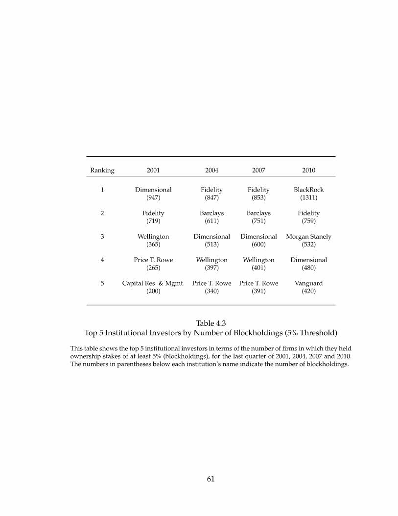
Ranking 2001 2004 2007 2010

1 Dimensional Fidelity Fidelity BlackRock(947) (847) (853) (1311)

2 Fidelity Barclays Barclays Fidelity(719) (611) (751) (759)

3 Wellington Dimensional Dimensional Morgan Stanely(365) (513) (600) (532)

4 Price T. Rowe Wellington Wellington Dimensional(265) (397) (401) (480)

5 Capital Res. & Mgmt. Price T. Rowe Price T. Rowe Vanguard(200) (340) (391) (420)



61

Ranking 2001 2004 2007 2010

1 Fidelity Fidelity Fidelity Fidelity(522) (635) (655) (584)

2 Dimensional Barclays Dimensional BlackRock(428) (247) (367) (477)

3 Wellington Wellington Price T. Rowe Morgan Stanely(243) (242) (256) (414)

4 Price T. Rowe Price T. Rowe Wellington Price T. Rowe(173) (231) (255) (247)

5 Franklin Resources Dimensional Barclays Dimensional(106) (217) (197) (229)



62

TXRH

TDG

LAYN

LGCY

CITZ

UAL

WPRT

HOLI

ATDN

NVEC

SNSR

NBTF

ICBN

UTIX

RWV

VMW

BGU

REXX

TYO

JDAS

SMB

PROV

WAMU

CSFS

EQR

CHKE

SPPI

MDU

PMFG

BANR

TOD

DPDW

CAW

DLOV

LTD

ALE

DOG

GPSN

PSID

TCRD

AKRX

ICE

MBA

ALCO

ENS

URG

SNV

AMNF

EBF

PRMX

GLW

CHCR

SCHP

ASGR

EVBN

NOBH

MSCI

INCT

EPD

VSS

ISIL

DNME

ROP

ZN

NEI

INCB

EVI

NFLX

RBPA

PDII

DBN

UMPQ

WTBA

CGLA

BBAL

CNIT

ARG

LINT

ITPO

SUNV

MLVF

CWB

SMWK

BSTC

HDWR

IAG

ISBC

CRFN

VPLM

HKFI

RYL

SEB

LBIX

CTBC

PCY

BCO

HEV

IMCB

AEBF

CRDC

EMIF

GWX

COVR

KDUS

DGII

GSTFBCM

DMLP

SMTX

SDK

DGEN

RPRX

KALU

FXR

CMP

HUBB

BRS

ATHR

FDEF

FLS

MPAC

CT

FPFX

CTGX

BVSN

RXD

UBP

ZUMZ

CSHD

A

ENOC

EGMI

EDR

BAS

LKQX

FPBI

AGL INDB

PBIO

BMRC

KCE

ENG

LGL

GENZ

CBM

SPLS

MWFS

GRC

IGC

BRF

MBRG

TWRA

GR AUY

MHS

PXN

MDXG

QBC

ALV

MFE

TFSL

TMF

ANSS

FSP

IGTE

SNPS

XGC

VGIT

CHIQ

EPL FULL

LULU

JKHY

AFL

MDEA

IHSV

WPO

DSCM

PNRG

BW

RSKI

WLFC

ASHG

FINL

FORD

FNBN

LFGP

TITN

TRDM

TMHPZD

LOTS

YSI

AFSI

EFOT

RRC

MMLP

TIS

TOO

NYMT

NVIC

AACC

DIMC

UCD

GSC/

SPA

GCI

CTO

ESMC

NANM

KBAL

SCSC

FCHI

BRCI

VSEC

NNSR

N

CTCM

FCF

AOI

INAP

EVR

ADEP

TRMB

VCR

IBI

TRS

STLD

BSQR

QTM

BIO GE

GGC

SRSL

PDEX

BBBY

EIRL

ROC

SCAY

BLIN

DNRR

LECO

DRN

ELGX

UTIW

TUZ

AOR

WST

OABC

MRPI

HEAT

EGT

LLEN

NBL

RNOW

AETI

ALY

ATI

FSII

MMSI

COOL

VITA

CMOH

USG

WCN

TRT

RLOG

TRI

THMR

TRNO

GEX

NTSC

ZGCO

FECO

TPCA

VEA

ZOOG

MTSC

UCC

CBMI

SCIA

MUB

BWC

DSXJ

CBS

HPJ

MDTH

PHB

SKYF

SIL

STLONXX

FBAK

SUI

USTKFY

ADRE

MAIN

SIEB

OTEX

XRU

MEE

BONT

AEP

XFN

ONBI

CPHD

PVFC

PBIB

BCAR

SFEG

CPCF

PLAB

OMCL

IGN

PSE

CNHL

SHZ

TPC

TTT

SCVL

TQNT

ARCW

AMOK

ELON

CNCIART

OPXT

AFP

HEWA

LZ

TSOH

CXW

JAS

ZHNE

BBGI

SF

ABT

GSON

IWEB

EHTH

COL

SEF

LSTR

MYY

CCF

ELX

ABMC

MDVT

CARV

KMX

SXT

CUBN

RTM

BOJF

KVHI

TNAV

MDW

CART

GII

CHUX

AKR

HDSNGIFI

PQB

DEMO

FCVA

SKVY

DCDC

EBIG

PG

CSCO

AMG

VCSH

TWC

EGLE

SMSI

CYTK

MGOL

KOP

MFB

GRAN

PAET

BRKR

ISYS

NEN

WINN

AMIC

VCLT

WFD

COBZ

ASNL

ERTSDXCM

TBBK

LMLP

VTHR

QUIK

LPHI

BNVI

SNBC

FSOF

TAYC

CRRC

LYTS

CVLT

SWKS

ALXN

LSFG

BKF

BMNM

VIRC

VTWG

ENYC

Y

CKXE

CICS

RCMT

TGIS

HAP

TWX

NHTB

TTEC

HURC

ABKF

TEAM

SJT

DRRX

BMY

PWX

ADZR

CMS

STJ

GFGU

BBEP

CNQ

BIEL

PDMAZZ NXST

UTMD

GPIC

RTR

FMR

LPS

CRDS

NDN

KAD

AIMM

IAU

VNBC

CHK

SPRO

ASBI

PFG

AMPL

BPUR

GHDX

CWBK

HLYS

BLD

ORMP

FFIV

LG

FGD

CSS

AQUA

MRIN

PBM

ASTEORB

LFYC

SQI

AEMD

JBL

AADR

COF

JFT

UPV

INFI

ACM

WEN

ECBE

IVOG

INTU

NANX

VCMP

DVR

DYSL

PXH

DTG

COPR

FSFG

WBSN

TSPT

SUPX

TMK

WLP

SHLO

FFG

TRC

GLF

TECD

SGU

TDH

EXR

HOLL

UWM

QLIKEXPR

TPI

SRX

BXC

XYNH

MLKN

XLES

LHRP

GTLT

UNB

HERC

RHT

SCS

WRTL

FIBP

IIIN

MNRK

CHBT

VPFG

AIT

VTI

ZIOP

MZIA

EMIS

KIWB

DTN

KIE

AIM

GWDC

FHCO

NIVM

WLDN

BEAT

IBXG

RFMI

IACH

OPOF

PUDA

FVD

MCBF

MOS

JWA

SOQ

AMOT

ANDR

EQIX

MHO

ZQK

ARFR

FEIC

ROL

GTXI

SDRG

RDIB

JCO

SPMD

VIOV

TRH

PTSX

MESA

NAK

MCO

LAG

EZJ

VVTV

SMA

ZAAP

IWS

NVLS

AMST

LITH

WNR

XXCG

FAST

TLH

CLRO

PBW

PLM

CRY

TSTA

ICN

RL

ANH

CHRS

UVSP

SEMG

HTCHCPWM

MKBY

CTQN

TMEN

FAA

EEG

ACUS

UNM

EXAM

BRKB

GFED

COMV

PLG

SUSQ

KLD

CRDN

ANR

NWL

SKH

BEXP

WITM

ICUI

ALT

MBRK

STKL

MGA

USM

FDO

ICH

IAAC

ERY

LCNT

DDE

GVP

PNDM

VTWV

MCHX

TSO

QCLN

USU

DYMT

SYMX

RLH

JSDA

DHIL

KMGB

SOYL

CAST

DRC

HEP

AOK

DPW

DAKM

RWR

AFFX

CPE

FSCI

ABIO

PICO

EPB

CLWA

OREX

BBG

RGNC

JAVO

TRUE

SWTS

FMAR

AMP

DRCO

CCAA

NEP

FFI

USAU

ECSL

CMZP

PNX

EPU

CUO

EBAY

YHGG

WLB

IGI

FFCH

LL

IRNS

ATTG

NCCI

BSUR

FLIC

PLPC

PNBC

PLA

AMRI

FPTB

HIFS

CLIOVLY

BNCN

RLRN

PAGG

CHGS

DPL

RCII

GOOG

ALIM

ENZ

ITRI

FACE

FDX

PLCM

CRNM

BTU

SPEC

BNX

BHE

IUSN

PZZI

PENX

KO

POCC

JFBC

CWIBIOC

UIS

STRT

GACF

ICCC

BECN

CVTR

TWTR

TBT

GACH

DDXS

EGHT

FCCO

EDGW

PII

ZZ

ITB

HZO

ELOY

GRA

CMRO

MUNI

HOC

PXQ

APBL

MUAA

CXBT

FIG

PCTI

SUR

NHC

TSTF

CHIB

BVBC

NSR

USEG

WEBC

MCWE

CVCY

GRID

CRVP

MELA

MDCE

ITT

OME

WTM

UKF

NPBC

ULQ

CIL

QDEL

LOGM

BIL

MGYR

EPCT

SMN

CIX

UVUM

IMN

BCPC

USOO

VNM

XRAY

CRS

OLEP

SJW

ARIA

PTIX

SIX

CSBC

KKR

NUCL

NEGI

MCOA

LCAP

NLCI

BRKL

PFF

AMR

HAO

MCBC

SWS

GBTR

DIG

SNGX

EEP

PSBH

SGS

QID

JAHI

ESBK

DXPE

NST

BRN

ALIF

CMG

TIBX

DSPG

BLK

GWW

AAXJ

FXPT

CPST

SPU

PFM

HYG

OPHC

FORR

AUTH

KEYN

ESA

EMAK

PAYD

UTR

CSBK

PCLN

PSTL

ZSTN SSD

BRCO

SGI

CNBC

HBCP

JWB

IWR

LTPZ

CNX

MBND

SLW

FPBN

PFBC

SNVP

FTK

TLEO

BJRI

MCRO

EESV

RBCN

TSBK

CPT

AMBZ

TMV

AEY

HLIT

NHP

CYLU

FNFG

TOBC

LTHU

BDR

HGR

PMA

LQMT

ID

MMPI

IPHS

FMBI

TD

BJGP

AMJ

IRET

CHG

PFCB

FNSI

KYZN

UYM

NENE

CTCT

WCII

SCHN

L

USAT

LWLG

CSNT

VOT

GYRO

SLGD

NOVS

AIA

ZIXI

SIGA

APH

LXRX

CIA

CNWH

TRV

UBD

KRE

MCRI

TEAR

VDE

AF

PSRU

BAMM

RA

MOBL

DSW

JPM

KOSS

SKOR

PAY

CHRW

CSV

FTC

PEBO

FCX

SPIR

JLL

ES

TLGD

BLCB

KND

CRYP

GXF

RWW

WSBC

CIT

PICB

CLXM

AGP

ESS

CHMO

DYAX

SLRK

IFNY

PLT

HCSG

PERF

DVNT

TIP

NPNT

ISH

SCI

FRI

ETCC

GHL

WMS

SAFM

DIS

WMCR

AOB

HCCI

PSWS

ICLN

MOFG

FCSE

CZIC

DCBR

DVIN

BDCO

SCZ

MAR

UGL

TCK

AIQ

NTME

FXF

VSPC

PPBN

CXDC

PETS

EDIG

RBNF

CRAY

NCYB

UBSH

YAVY

ONEQ

PRO

RDEA

DLM

WPP

KNOL

UTI

ECNG

LNDC

RYE

NVE

CNRD

AVEO

AHT

Figure 4.1Shareholder Network (Random Sample of 1000 Companies in 2010Q4)

This figure shows a plot of a sample of 1000 companies in the network of firms in 2010Q4. Theedges are generated by common institutional shareholders with ownership stakes of at least 5% ina pair of firms. The layout of the network is calculated using a Fruchterman-Reingold algorithm.The size of the circles is proportional to the logarithm of a company’s market capitalization. Thecolor represents the number of connections of the company, with colors closer to blue indicatingless connections, and colors closer to red indicating more connections.

63

0

0.05

0.1

0.15

0.2

0.25

2001 2004 2007 2010

3% Threshold 5% Threshold 7% Threshold

Figure 4.2Evolution of the Density of the Network of Interlocking Shareholdings: All Firms

Source: SEC through Thomson Reuters and author’s calculations.

64

0

0.1

0.2

0.3

0.4

0.5

0.6

0.7

2001 2004 2007 2010


Figure 4.3Evolution of the Density of the Network of Interlocking Shareholdings: Largest

3000 Firms


65

0

0.1

0.2

0.3

0.4

0.5

0.6

0.7

0.8

0.9

2001 2004 2007 2010


Figure 4.4Evolution of the Density of the Network of Interlocking Shareholdings: Largest

500 Firms


66

0

0.1

0.2

0.3

0.4

0.5

0.6

0.7

0.8

2001 2004 2007 2010


Figure 4.5Fraction of Firms with At Least one Blockholder: All Firms


67

0

0.1

0.2

0.3

0.4

0.5

0.6

0.7

0.8

0.9

1

2001 2004 2007 2010


Figure 4.6Fraction of Firms with At Least one Blockholder: Largest 3000 Firms


68

0

0.1

0.2

0.3

0.4

0.5

0.6

0.7

0.8

0.9

1

2001 2004 2007 2010


Figure 4.7Fraction of Firms with At Least one Blockholder: Largest 500 Firms


69

0

0.1

0.2

0.3

0.4

0.5

0.6

0.7

0.8

0.9

1

2001 2004 2007 2010


Figure 4.8Fraction of Connections Generated by the Top 5 Institutional Investors


70

0

0.1

0.2

0.3

0.4

0.5

0.6

0.7

2001 2004 2007 2010

Top 1 Top 5 Top 10 Top 20

Figure 4.9Fraction of Firms Owned by the Top x Institutional Investors: 3% Threshold


71

0

0.1

0.2

0.3

0.4

0.5

0.6

2001 2004 2007 2010




72

0

0.05

0.1

0.15

0.2

0.25

0.3

0.35

0.4

2001 2004 2007 2010




73

0

0.1

0.2

0.3

0.4

0.5

0.6

0.7

0.8

0.9

1

2001 2004 2007 2010


Figure 4.12Fraction of Firms Owned by the Top x Institutional Investors: 3% Threshold,

Largest 3000 Firms


74

0

0.1

0.2

0.3

0.4

0.5

0.6

0.7

0.8

2001 2004 2007 2010



Largest 3000 Firms


75

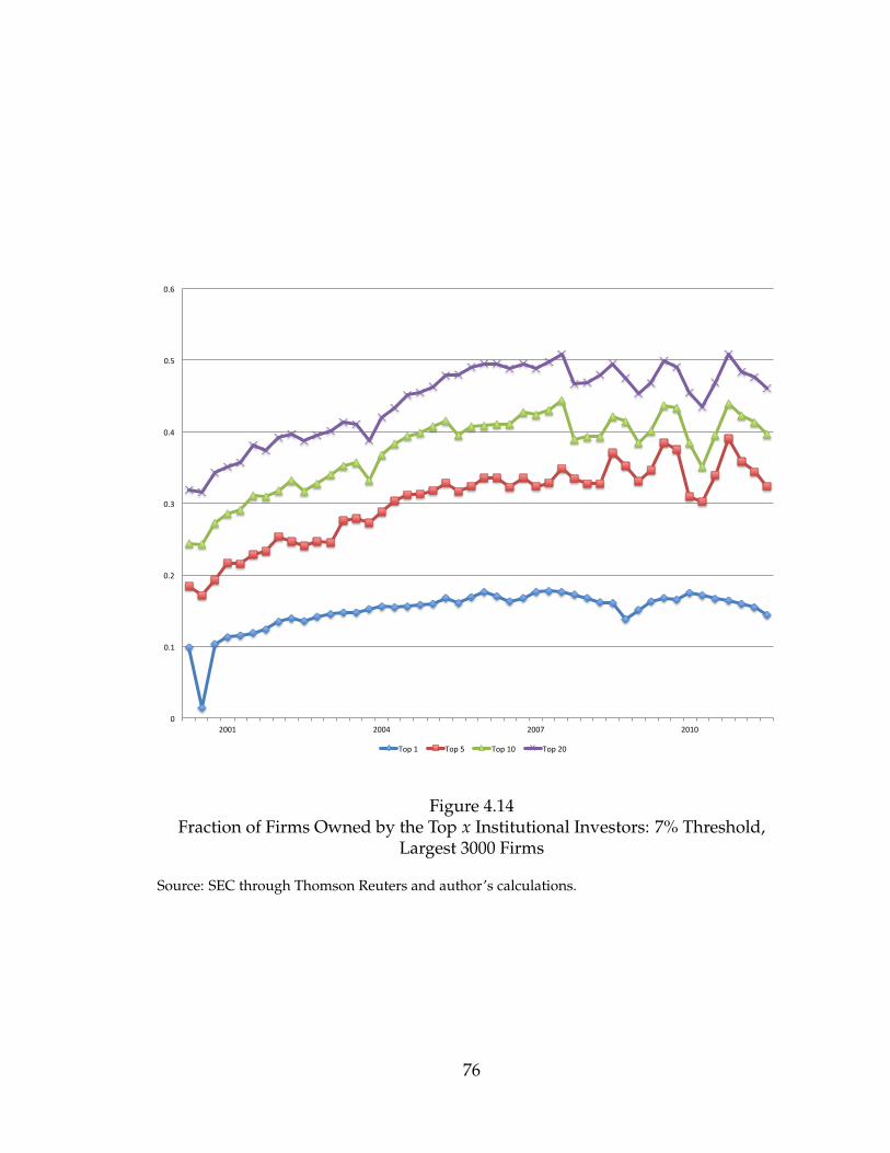
0

0.1

0.2

0.3

0.4

0.5

0.6

2001 2004 2007 2010



Largest 3000 Firms


76

10−6

10−5

10−4

10−3

10−2

10−1

100

10−4

10−3

10−2

10−1

100

Fraction of market cap held k

Fra

ctio

n of

inst

itutio

ns P

k hav

ing

a fr

actio

n of

k o

r gr

eate

r

20002011

Figure 4.15Cumulative Distribution Function for the Value of the Portfolios of Institutional

Investors as a Share of Total Market Capitalization: 2000 and 2011


77

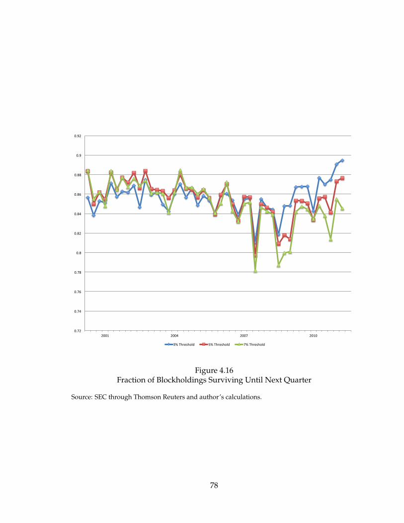
0.72

0.74

0.76

0.78

0.8

0.82

0.84

0.86

0.88

0.9

0.92

2001 2004 2007 2010


Figure 4.16Fraction of Blockholdings Surviving Until Next Quarter


78

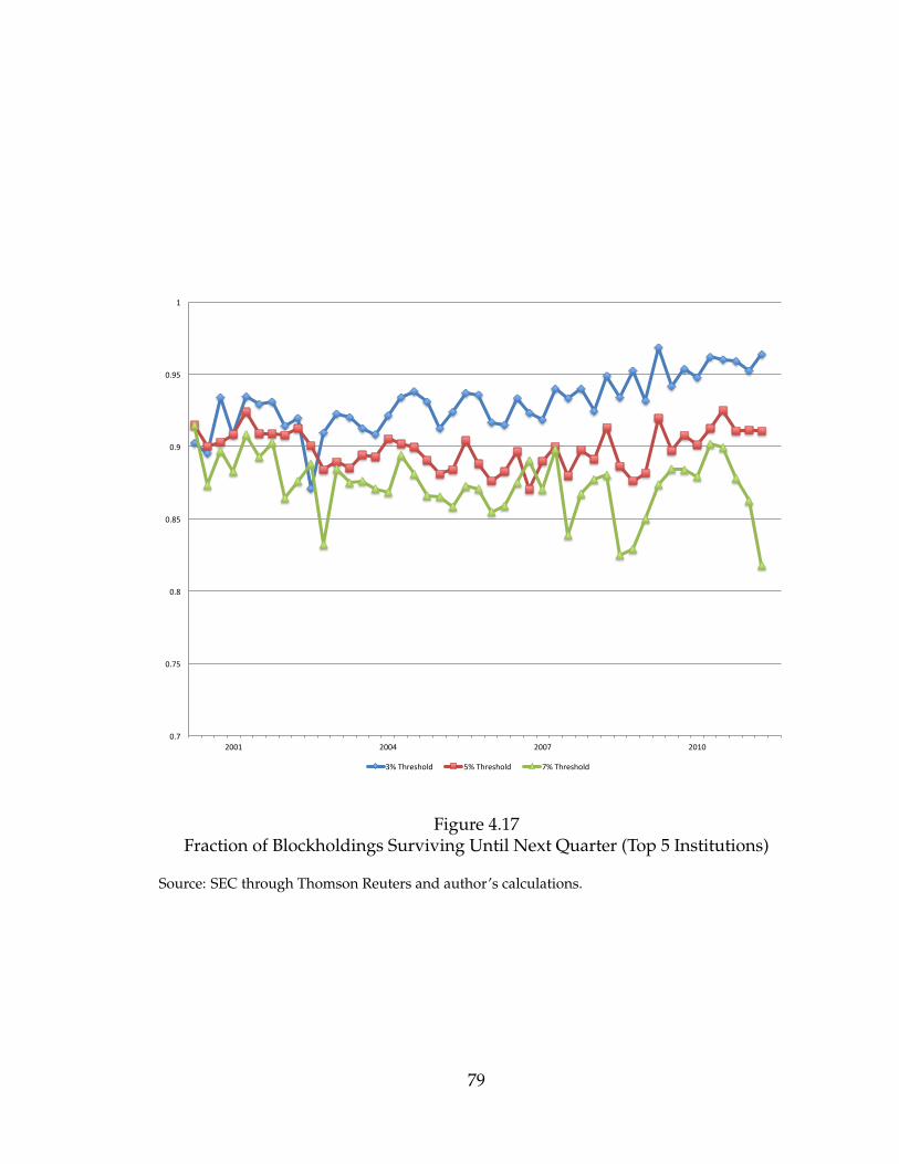
0.7

0.75

0.8

0.85

0.9

0.95

1

2001 2004 2007 2010


Figure 4.17Fraction of Blockholdings Surviving Until Next Quarter (Top 5 Institutions)


79

100

101

102

103

104

10−4

10−3

10−2

10−1

100

Degree k

Fra

ctio

n of

firm

s P

k hav

ing

degr

ee k

or

grea

ter

20002011

(a) 3% Threshold

100

101

102

103

104

10−4

10−3

10−2

10−1

100

Degree k

Fra

ctio

n of

firm

s P

k hav

ing

degr

ee k

or

grea

ter

20002011

(b) 5% Threshold

100

101

102

103

104

10−4

10−3

10−2

10−1

100

Degree k

Fra

ctio

n of

firm

s P

k hav

ing

degr

ee k

or

grea

ter

20002011

(c) 7% Threshold

Figure 4.18Cumulative Distribution Functions for the Degrees of the Shareholder Network at

Different Thresholds: 2000 and 2011


80

0

0.1

0.2

0.3

0.4

0.5

0.6

Tex-les &

App

arel

Transporta-o

n

Airline

s

Insurance

Pape

r & Forest P

rodu

cts

Semicon

ductors

U-li-es: W

ater-‐Electric-‐Gas

Automob

iles

Food

& Restaurants

Construc-o

n & Engineerin

g

Chem

icals

Machine

ry & Equ

ipmen

t

Aerospace

Retail & Con

sumer Goo

ds

Consum

er Services

Med

ia

House Wares & Hou

seho

ld Item

s

Tobacco

Packaging

Electrical & Electronics

Compu

ter H

ardw

are SoSw

are and Services

Healthcare

Telecommun

ica-

ons

Waste & Enviro

nmen

t Managem

ent

Publish

ing & Prin

-ng

Leisu

re Travel &

Lod

ging

Beverages

Investmen

t Services

Agriculture

Energy and

Fue

ls

All ind

ustries

Indu

stria

l Manufacturin

g

Real Estate

Financial Services

Misc

ellane

ous

Banks &

Savings Ins-tu-o

ns

Unkno

wn

Metals &

Mining

Figure 4.19Industry Sub-Network Densities in 2011: 3% Threshold


81

0

0.05

0.1

0.15

0.2

0.25

0.3

0.35

Pape

r & Forest P

rodu

cts

Airline

s

Tex;les &

App

arel

Construc;o

n & Engineerin

g

Transporta;o

n

Food

& Restaurants

Chem

icals

Semicon

ductors

Consum

er Services

Insurance

U;li;es: W


Agriculture

Machine

ry & Equ

ipmen

t


Automob

iles

House Wares & Hou

seho

ld Item

s

Aerospace

Retail & Con

sumer Goo

ds

Investmen

t Services

Compu

ter H

ardw

are SoPw

are and Services

Healthcare

Tobacco

Publish

ing & Prin

;ng

Packaging

Indu

stria

l Manufacturin

g

All ind

ustries

Waste & Enviro

nmen

t Managem

ent

Leisu

re Travel &

Lod

ging

Telecommun

ica;

ons

Med

ia

Beverages

Energy and

Fue

ls

Banks &

Savings Ins;tu;o

ns

Unkno

wn

Real Estate

Misc

ellane

ous

Financial Services

Metals &

Mining



82

0

0.02

0.04

0.06

0.08

0.1

0.12

0.14

0.16

Airline

s

Construc5o

n & Engineerin

g

Food

& Restaurants

Consum

er Services

Tex5les &

App

arel

Investmen

t Services

Transporta5o

n

Semicon

ductors

Automob

iles


House Wares & Hou

seho

ld Item

s

Healthcare

Retail & Con

sumer Goo

ds

Insurance

Publish

ing & Prin

5ng

Agriculture

Chem

icals

Compu

ter H

ardw

are SoKw

are and Services

Pape

r & Forest P

rodu

cts

Machine

ry & Equ

ipmen

t

Energy and

Fue

ls

Aerospace

Leisu

re Travel &

Lod

ging

All ind

ustries

Indu

stria

l Manufacturin

g

Telecommun

ica5

ons

Med

ia

Beverages

Banks &

Savings Ins5tu5o

ns

Unkno

wn

Real Estate

Waste & Enviro

nmen

t Managem

ent

Misc

ellane

ous

U5li5es: W


Metals &

Mining

Financial Services

Packaging

Tobacco



83

Chapter 5

Common Shareholders and

Interlocking Directorships

5.1 Introduction

I this chapter, I study the empirical relationship between common ownership and

interlocking directorships. I estimate a gravity equation model for the probability

that a pair of firms will have a common director, as a function of the geographic

distance between the firms, their sizes, and a set of covariates, including measures

of common ownership between the firms. The main finding is that, robustly across

several measures of common ownership, firm pairs with higher levels of common

ownership are more likely to share directors. Also, their distance in the network

of directors is smaller on average. Consistent with the “gravity” interpretation,

larger firms are more likely to share directors, and firms that are geographically

more distant are less likely to share directors.

84

While past work has studied networks of interlocking directorships, this chap-

ter is the first to study the determinants of interlocks at the firm-pair level using a

gravity equation.1

The evidence presented in this chapter suggests that institutional investors play

an active role in corporate governance. In particular, it supports the hypothesis

that institutional shareholders have influence on the board of directors. Other

studies have also found evidence that institutional investors play an active role in

governance and can influence, among other things, executive pay and turnover.2

Recent papers have studied the effect of common ownership by institutional in-

vestors on merger and acquisition decisions.3

5.2 Data Description

Data on boards of directors for US firms is available from the Corporate Library.

The frequency of the data is yearly, and the data start in 2001 and 2010. The data on

institutional ownership and market capitalization, as in Chapter 3, is from Thom-

son Reuters. To convert the quarterly ownership data to a yearly frequency, I use

the observations from the last quarter of each year. Data on zip codes, which are

necessary to calculate the geographic distance between firms, and for SIC industry

codes, is available from Compustat.

Table 5.1 shows summary statistics for the merged dataset. The number of

firms with available data for director interlocks has increased substantially over

time. In 2001, only 1,049 firms had data for directors, institutional shareholders,

1For a sample of the literature on interlocking directors in sociology, see Domhoff (1967) andMizruchi (1996). There has been some recent interest in the finance literature on the relationshipbetween director interlocks and corporate finance decisions, such as the work of Stuart and Yim(2010), Cai and Sevilir (2011), and Cukurova (2011).

2See, for example, Agrawal and Mandelker (1990), Kaplan and Minton (1994), Hartzell andStarks (2003), and Kaplan and Minton (2008).

3See Matvos and Ostrovsky (2008) and Harford et al. (2011).

85

market capitalization, industry, and zip codes. For 2010, the number was 2,597.

The number of directors represented in the sample increased from 9,907 to 39,991.

Thus, the average number of directors per firm has increased. The same is true for

blockholdings, which throughout the chapter are defined as holdings above the 5%

threshold. The number increased from 1,866 in 2001 to 6,804 in 2010, an increase

more than proportional to the increase in the number of firms.

For a pair of firms, a director interlock is generated if there is at least one direc-

tor that sits on the boards of both firms. The number of director interlocks in the

sample increased from 1,999 to 12,939. A shareholder interlock for a pair of firms

is generated if there is an institutional shareholder who owns at least 5% in both

firms. The number of shareholder interlocks increased from 55,963 to 1,071,738.

The large increases in interlocks, both in the directors and shareholder sampled

networks, should by themselves not be too surprising, since the number of inter-

locks is expected to grow more than proportionally as the sample size increases.

Figure 5.1 shows a plot of the network of interlocking directors in 2010. The

size of the circle is proportional to the log of market capitalization. The color varies

with the number of connections of the firm, with colors closer to blue indicating

less connections, and colors closer to red indicating more connections. The layout

of the plot is calculated using a Fruchterman-Rheingold algorithm. There is a clear

relationship between firm size and number of connections, which should not be

surprising given that larger firms tend to have more directors, and therefore more

possibilities for interlocks. Thus, large firms tend to be at the center of the net-

work. Unlike the network of interlocking shareholders, whose plot was shown in

Chapter 3 (Figure 3.1), there are no salient clusters in the network of interlocking

directors.

Figure 5.2 shows the cumulative distribution of degrees for the network of in-

terlocking directors in 2001 and 2010. The degrees in the sample have increased,

86

but this is not surprising given the increase in the number of firms in the sample.

There is no evidence of fat tails in the degree distribution for either period.

5.2.1 Weighted Measures of Common Ownership

Defining two firms as having common owners if there is an institutional share-

holder having more than x percent in both has the advantage of conceptual sim-

plicity. However, it leaves out large amounts of useful information. For example,

if a shareholder has 20% in two firms, the 5%-threshold measure is the same as

if the shareholder only had exactly 5% in each firm, despite the fact that having

a shareholder with 20% in two firms clearly represents a higher level of common

ownership for that pair of firms. Conversely, if there is a shareholder having 4.99%

in both firms–and all the other shareholders have less than 5% in both firms–then

the measure will be zero, the same as if the firms had completely separate owners.

In this chapter, I will argue in favor of three new measures of common owner-

ship that can take a continuum of values. Thus, each of these measures defines a

weighted network of interlocking shareholdings.

Maximin

The first new weighted measure of common ownership for a pair of firmsi, j that

I propose to use is the “Maximin”, defined as

Maximinij = maxg∈G

min [sgi, sgj]

,

where G is the set of shareholders of both firms, and sgi is the percentage of firm i

owned by shareholder g.

Thus, is a shareholder has 20% of firm i and 20% of firm j, and all the other

shareholders do not have shares in both firms, the Maximin for that pair is .2. If

87

instead the common shareholder had 5% in both firms, the Maximin would be

.05. If the common shareholder had 4.99%, the Maximin would be .0499. Thus,

this measures solves two problems of the common shareholder dummy measure:

common ownership not increasing for stakes above 5%, and falling to zero for

common stakes just below 5%.

Intuitively, the Maximin is the largest threshold x for which the common own-

ership dummy would be equal to one. That is, suppose the maximin is .08. Then

a common ownership dummy with a threshold of x percent would equal one for

x ≤ .08 and zero for x > .08.

Thus, the Maximin has several benefits as a measure of common ownership. It

is almost as intuitive as the common shareholder dummy. It avoids the arbitrari-

ness of setting a threshold for common ownership. It avoids the discontinuity at

the threshold. And, finally, it assigns a higher level of common ownership to firm

pairs with shareholders that hold larger blocks of both firms.

Sum of Mins

While an improvement with respect to the common ownership dummy, the Max-

imin measure of common ownership still has drawbacks. For example, consider a

pair of firms i, j has one common shareholder with 5% in both firms. Now con-

sider another pair of firms, k, l, with four common shareholders, each owning

5% of both firms. The Maximin measure would be .05 for both pairs of firms, even

though the total amount of stock that is commonly owned for the second pair is

four times higher than for the first pair. The reason is that the Maximin only fo-

cuses on the shareholder with the largest block of stock in the pair of firms, while

throwing out information from all the other shareholders.

88

A second new measure of common ownership that includes information on all

the common shareholders, is the “Sum of Mins”, defined as

Sum o f Minsij = ∑g∈G

min [sgi, sgj].

One way to think about this measure is the following. One can think of a pair

of firms i, j as having several common ownership links, each generated by a

different shareholder. The intensity of the link generated by shareholder g can be

captured by the min [sgi, sgj]. The Sum of Mins summarizes all of these links by

adding them. For the example above, the Sum of Mins would be .05 for the pair of

firms i, j, and .2 for the pair of firms k, l.

Thus, the Sum of Mins also provides an intuitive weighted measure of common

ownership, and addresses a potential problem with the Maximin measure. How-

ever, the strength of the Sum of Mins in terms of capturing the links generated by

all the shareholders can also be a drawback in some applications, in particular if

one would want the measure to penalize for a low concentration of ownership.

With the Sum of Mins, the measure is the same if there is one owner having 100%

in both firms or 100 owners each having 1% in both firms. The Maximin, on the

other hand, imposes a very high penalty for lack of ownership concentration: it ig-

nores all shareholders except the one that generates the connection with the highest

weight.

Inner Product

A third measure that imposes a penalty for lower concentration that is lower than

the Maximin but higher than the Sum of Mins is the (unnormalized) “Inner Prod-

uct”:

Inner Productij = ∑g∈G

sgisgj.

89

Like the Sum of Mins, the inner product sums the weights of the connections

generated by all the common shareholders, but in this case the weight is defined

by the product of the percentage ownership stakes rather than the minimum. The

product yields values that are more than proportionally higher for more concen-

trated ownership stakes. Thus, the Inner Product measure “rewards” ownership

concentration, while the Sum of Mins does not. For example, consider a pair of

firms i, j such that one shareholder owns 100% of both firms. Both the Sum of

Mins and the Inner Product are equal to one. Now consider another pair k, l

such that two shareholders each have portfolios with 50% of both firms. The Sum

of Mins for k, l is still equal to one, even though the ownership is less concen-

trated. The Inner Product, however, equals .52 + .52 = .5. If, instead the pair were

owned by four shareholders each owning 25% of both firms, the Sum of Mins

would still be one, while the Inner Product would be 4× .252 = .25. Thus, for a

pair of firms completely held by the same owners, splitting the ownership stakes in

half, which reduces ownership concentration without changing the fact that firms

are commonly owned, also halves the Inner Product measure of common owner-

ship, while having no effect on the Sum of Mins.

For example, if a shareholder owns 5 percent of firm i and 5 percent of firm

j, then the weight of the connection generated by that shareholder is 0.0025. If

a shareholder owns 10 percent in both firms, the weight of the connection is .01,

which is four times higher. In this sense,

The inner product of a firms with respect to itself is actually the Herfindahl

measure for ownership concentration. If one defines the matrix S containing sgi

in row g and column i, then the ownership concentration Herfindahl’s will be the

diagonal elements of S′S, and the common ownership Inner Product measures will

be the off-diagonal terms.

90

5.2.2 Firm-Pair Level Variables

Table 5.2 shows summary statistics for the variables at the firm-pair level that will

be used in the econometric analysis. There are 21,008,282 firm pair-year observa-

tions.

The common director dummy, already described, has a mean of .003427, indi-

cating that .34% of firm pairs (pooling all years together) have a director interlock.

The distance in the network of directors is the shortest path between to firms, and is

calculated using a Breadth-First Search algorithm. The average distance is slightly

above 4. The number of observations for distance is somewhat smaller than the

total because for some pairs the observed distance is infinite.

The common ownership variables were described in the previous section. For

the purposes of calculating the weighted measures of common ownership I restrict

the sample to holdings of at least 1% of outstanding stock. Approximately 22.6%

of the pairs in the sample have a common shareholder at the 5% threshold. The

average Maximin is 3.9%, the average Sum of Mins is 10.6%, and the average Inner

Product is .00572.

To control for the average size of a pair of firms, I use the the logarithm of the

product of the market capitalizations, in millions of 2001 dollars. The average of

the log of the product of market capitalizations is approximately 13.8. Combining

the zip codes with data on latitude and longitude I calculate the geographic dis-

tance between two firms using a Harvesine algorithm. The average distance of the

firms in the sample is 929.18km, with a minimum distance of zero and a maximum

distance of 4,727.88km. I also calculate a dummy for whether two firms are in the

same industry at the SIC 3-digit level, and a dummy for whether they are both in

the S&P500. Approximately 2.16% of the firm pairs are in the same industry, and

4.24% of the pairs are both in the S&P500.

91

Table 5.3 shows the correlation between the different measures of common

ownership. All the measures are highly correlated with each other. The measure

that is most highly correlated with the common shareholder dummy is the Max-

imin, with a correlation coefficient of 73%. The measure that is least correlated with

the common shareholder dummy is the Sum of Mins, with a correlation coefficient

of 58%. All the correlations between the Maximin, Sum of Mins, and Inner Prod-

uct are above 80%. The highest correlation is between the Inner Product and the

Sum of Mins, with a correlation coefficient of more than 88%. The Inner Product is

more highly correlated with the Sum of Mins or the Maximin than the last two are

with each other, supporting the idea that the Inner Product is an “intermediate”

measure in terms of how much it rewards ownership concentration.

5.3 A Gravity Equation for Director and Shareholder

Interlocks

In this section, I estimate “gravity” equations for the probability of director inter-

locks, distance in the directors’ network, and for measures of common ownership,

modeling these variables in terms of the product of the sizes of the firms in the

pair, their geographic distance, and other covariates. The basic specification for

the zero-one variables is

P(Yij,t = 1) =

Λ(β0 + β1Log(MarketCapi,t ×MarketCapj,t) + β2GeographicDistanceij,t + γXij,t),

where Yij,t represents either a dummy for common directors or for common share-

holders, Xij,t is a vector of controls, and Λ is the logistic function. For the continu-

ous variables (i.e. distance in the network, and the weighted measures of common

92

ownership), the basic specification is

Yij,t =

β0 + β1Log(MarketCapi,t ×MarketCapj,t) + β2GeographicDistanceij,t + γXij,t + εij,t.

Table 5.4 shows the results of Logit regressions with the common director

dummy and common shareholder dummy as dependent variables. Larger firms

have a significantly higher probability of having a common director, and a signif-

icantly lower probability of having a common institutional shareholder at the 5%

threshold. Firms that are geographically more distant have a significantly lower

probability of having a common director, and a significantly higher probability of

having a common institutional shareholder. Firms that are in the same Industry

at the SIC 3-digit level have significantly higher probabilities of both having a

common director and a common institutional shareholder. Firms that are both in

the S&P500 have a higher probability of interlocking directors. When controlling

for the log product of firm sizes using only a linear term, firms that are both in the

S&P500 have a lower probability of interlocking shareholders. However, when

including a cubic b-spline in the log product of firm sizes, the effect of both firms

being in the S&P500 is positive. The b-spline used in all the regressions in this

chapter has five knots: at the 10th, 25th, 50th, 75th, and 90th percentiles.

Figure 5.3 shows the estimated probability of interlocking directorships as a

function of the log product of market capitalizations, from regression (3) in Ta-

ble 5.4. The other regressors are fixed at their mean values, and the year is set to

2010. The effect of firm size on the probability of director interlocks is approxi-

mately zero for small firms, and is larger for large values of Log(MarketCapi,t ×

MarketCapj,t) than for values near the mean.

93

Figure 5.4 shows the estimated probability of interlocking shareholders at the

5% threshold as a function of the log product of market capitalizations, from re-

gression (4) in Table 5.4. The effect is nonmonotonic: the probability increases

as Log(MarketCapi,t × MarketCapj,t) increases up to approximately 12.5, and de-

creases for higher values.

Table 5.5 shows the results of linear regressions with the log of network distance

and weighted measures of common ownership as dependent variables. Standard

errors are clustered at the firm-pair level. Larger pairs of firms are closer in the

network of interlocking directors. When using the weighted measures of common

ownership, the effect of the log product of firm sizes is positive, however, whereas

the effect of size when using the common shareholder dummy was negative. Ge-

ographic distance has a positive effect on network distance, and it also increases

all measures of common ownership. Being in the same industry at the SIC 3-digit

level reduces expected network distance, and increases the expected value for all

measures of common ownership. Both firms being in the S&P500 reduces expected

network distance, and increases the expected value for all measures of common

ownership.

Figure 5.5 shows network distance as a function of Log(MarketCapi,t ×

MarketCapj,t). The other regressors are fixed at their mean values, and the

year is set to 2010. To obtain network distance I take the exponential of the pre-

dicted value for the log of network distance. Network distance falls monotonically

as a function of the product of firm sizes. The fall is somewhat less steep at the

lower range of Log(MarketCapi,t ×MarketCapj,t).

Figure 5.6 shows the expected Maximin as a function of Log(MarketCapi,t ×

MarketCapj,t). The effect of size is non-monotonic. The expected maximin in-

creases up to the log of the product of firm sizes equal to 13.8, which is close to

the mean, and then decreases for further increases in the log of the product of firm

94

sizes. However, the decrease is much less pronounced than in the case of the com-

mon shareholder dummy.

Figure 5.7 shows the expected Sum of Mins as a function of Log(MarketCapi,t×

MarketCapj,t). The effect of size in the case of the Sum of Mins is monotonic. The

increase in Sum of Mins is fastest for firm pairs below the mean of log product of

sizes. The increase in Sum of Mins becomes very slow, but still positive, for the

largest firm pairs.

Figure 5.8 shows the expected Inner Product as a function of Log(MarketCapi,t×

MarketCapj,t). The effect is non-monotonic. The pattern seems to be an interme-

diate of the cases of the Maximin and the Sum of Mins, again supporting the

idea that the Inner Product is “in between” these measures. The Inner Product

increases up to the log of the product of firm sizes equal to 15.6, and then decreases

for further increases in the log of the product of firm sizes. The decrease is slower

compared to both the case of the common shareholder dummy and the case of the

Maximin.

5.3.1 Have Director Interlocks Increased?

Has there been an increase in interlocking directorships over the past decade? A

nave look at the data would suggest that this is not the case. The solid line in

Figure 5.9 shows the raw probability that a randomly selected pair of firms in the

sample had an interlocking directorship for each year between 2001 and 2010. This

probability has fluctuated over time, but there is no clear trend. However, be-

cause the number of firms with data for boards in directors from Compustat has

increased over time, and, in particular, smaller firms are more highly represented

in later years, it is necessary to control the probabilities for firm size. The dashed

line shows the predicted probabilities using the gravity equation for director inter-

locks, setting the log product of firm sizes, as well as other regressors, equal to their

95

means. The only variable that varies over time are the year dummies. This shows

that for the average pair of firms the probability of a director interlock increased

during the period, almost doubling from .13% in 2001 to .23% in 2010. Note that

the predicted probability for the average firm pair is smaller than the raw proba-

bility at all periods. This is not surprising, since connections are much more likely

for very large pairs of firms compared to pairs of average log product of size.

5.4 Common Ownership and Interlocking Director-

ships

Are pairs of firms with higher levels of common ownership more likely to have

interlocking directorships? Are they closer together in the network of directors?

We can address these questions by introducing measures of common ownership

as explanatory variables in the gravity equation for director interlocks and for log

network distance.

Table 5.6 shows the results for the gravity equations using the common share-

holder dummy as the measure of common ownership. Column (1) shows the result

of a Logit model for the probability of interlocking directorships with a common

shareholder dummy at the 5% threshold, Log(MarketCapi,t ×MarketCapj,t), geo-

graphic distance, a dummy for the firms in the pair being in the same industry

at the SIC 3-digit level, a dummy for both firms being in the S&P500, and year

dummies. Having a common institutional shareholder has a positive and highly

significant effect on the probability that the firm pair has interlocking directors.

Column (2) shows the results of a similar regression, but adding interaction

terms for the common shareholder dummy and the same industry dummy, and for

the common shareholder dummy and the S&P500 dummy. The effect of common

96

ownership is larger for pairs that are in the same industry, and it is smaller for

pairs that are in the S&P500.

Column (3) shows the results of a regression similar to that in Column (2), but

adding a cubic spline in Log(MarketCapi,t × MarketCapj,t). The direction of the

results is unchanged, and the magnitude of the effect of common shareholders on

director interlocks is similar.

Column (4) shows the results of a Logit regression with firm-pair fixed effects.

Geographic distance, the same industry and S&P500 dummies, and the interaction

effects are dropped due to lack of within variation. The effect of common share-

holders on common directors is positive but not significant at 5% (the p-value is

approximately 12%).

Columns (5) to (8) show the results of analogous specification, but for linear

regressions with the log of distance in the network of interlocking directors as the

dependent variable, instead of a common director dummy. It should be noted that

the log of distance for the sampled network is an upwardly biased estimator of

the actual distance, since there are potential paths that could be shorter but are not

observed because they go through nodes that are outside the sample. The common

shareholder dummy has a negative and significant effect at 1% on the distance in

the directors’ network for all specifications. Being in the same industry makes the

effect of common shareholders stronger, while in the S&P500 reverses the sign of

the effect.

Table 5.7 shows the results for similar regressions, but using Maximin instead

of the common shareholder dummy. The results are similar. However, the positive

effect of Maximin on the probability of interlocking directors when using fixed ef-

fects is significant at 5% (Column 4). Another difference is that, in the log network

distance regressions, being in the same industry weakens the effect of Maximin in

Column (6), and is not significant in Column (7).

97

Table 5.8 shows the results using Sum of Mins as the measure of common own-

ership. The main results are similar. In this case the positive effect of Sum of Mins

on the probability of interlocking directors when using fixed effects is significant

at 1% (Column 4). Being in the same industry weakens the effect of common own-

ership on interlocking directors and on log network distance, as does being in the

S&P500.

Table 5.9 shows the results using the Inner Product as the measure of common

ownership. The main results, again, are similar. The positive effect of the Inner

Product measure of common ownership on the probability of interlocking direc-

tors with fixed effects is significant at 5% (Column 4). Being in the same industry

makes the effect of common ownership stronger in the common director regres-

sions, and weaker in the log of network distance regressions. Being in the S&P500

weakens the effect both in the common director and in the log of network distance

regressions.

Thus, the regression analysis does support the hypothesis that common owner-

ship has an effect on the network on interlocking directors. A plausible explanation

is that institutional shareholders have at least some power to influence who will

be on the board of the firms in which they hold blocks of stock.

5.5 Summary

In this chapter I showed evidence on the relationship between measures of com-

mon ownership and interlocking directorships. There is a positive relationship be-

tween the level of common ownership for a pair of firms and the probability that

the pair has interlocking directors, and a negative relationship between common

ownership and distance in the network of directors.

98

These results are robust across a range of measures of common ownership, in-

cluding several new weighted measures. The results hold even when controlling

for fixed effects. This suggests the presence of a causal relationship, although it

does not provide definitive evidence. Thus, the data support the hypothesis that

institutional shareholders have an active influence on the board of directors of pub-

licly traded US firms.

99

Year Firms Directors Blockholdings Director Interlocks Shareholder Interlocks

2001 1,049 9,907 1,866 1,999 55,963

2002 1,130 11,098 2,103 2,494 72,629

2003 1,286 13,725 2,256 3,508 87,240

2004 1,507 13,779 3,282 3,295 189,348

2005 1,576 14,407 3,693 3,363 206,140

2006 2,390 30,904 6,210 9,130 535,479

2007 2,557 34,427 7,137 10,785 604,136

2008 2,605 36,996 7,084 11,625 907,527

2009 2,733 40,161 6,681 12,858 1,025,909

2010 2,597 39,991 6,804 12,939 1,071,738


100

Variable Obs Mean Std. Dev. Min Max

Directors Network Variables

Common Director Dummy 21,008,282 .003427 .0584404 0 1

Distance in the Network 16,244,541 4.096688 1.140737 1 14

Common Ownership Variables

Common Shareholder Dummy 21,008,282 .2263921 .4184958 0 1

Maximin 21,008,282 .0390907 .0207413 0 .7607495

Sum of Mins 21,008,282 .1061435 .0622078 0 .7607495

Inner Product 21,008,282 .0057231 .0047606 0 .704425

Control Variables

Log(MarketCapi ×MarketCapj) 21,008,282 13.79712 2.455084 -1.491559 25.6797

Geographic Distance (km) 21,008,282 929.1822 635.7565 0 4727.881

Same Industry Dummy (SIC3) 21,008,282 .0216108 .1454089 0 1

Both in S&P500 Dummy 21,008,282 .0424458 .201604 0 1

Table 5.2Summary Statistics for Variables at the Firm-Pair Level

101

Common Shareholder Maximin Sum of Mins Inner ProductDummy

Common Shareholder Dummy 1.0000

Maximin 0.7366 1.0000

Sum of Mins 0.5795 0.8056 1.0000

Inner Product 0.6486 0.8654 0.8821 1.0000

Table 5.3Correlation Matrix for Common Ownership Variables

102

Common Dir. Common Sh. Common Dir. Common Sh.(1) (2) (3) (4)

Log(MarketCapi ×MarketCapj) 0.230*** -0.0457***(0.00397) (0.000335)

Geographic Distance -0.000978*** 3.07e-05*** -0.000982*** 3.57e-05***(2.05e-05) (1.26e-06) (2.04e-05) (1.26e-06)

Same Industry 1.346*** 0.221*** 1.330*** 0.245***(0.0303) (0.00541) (0.0307) (0.00536)

Both in S&P500 1.079*** -0.0497*** 1.026*** 0.472***(0.0250) (0.00479) (0.0280) (0.00516)

Constant -8.349*** -0.168*** -8.371*** 0.880***(0.0605) (0.00491) (1.702) (0.195)

Cubic Spline inLog(MarketCapi ×MarketCapj) No No Yes Yes

Year FE Yes Yes Yes Yes

Observations 21,003,082 21,003,082 21,003,082 21,003,082Robust standard errors in parentheses

*** p<0.01, ** p<0.05, * p<0.1

Table 5.4Gravity Equations for Common Directors and Common Shareholders (Logit)

103

Log

Net

wor

kM

axim

inSu

mof

Min

sIn

ner

Prod

uct

Log

Net

wor

kM

axim

inSu

mof

Min

sIn

ner

Prod

uct

Dis

tanc

eD

ista

nce

(1)

(2)

(3)

(4)

(5)

(6)

(7)

(8)

Log(

Mar

ketC

api×

Mar

ketC

apj)

-0.0

438*

**0.

0006

78**

*0.

0063

7***

0.00

0279

***

(5.5

4e-0

5)(3

.31e

-06)

(1.0

3e-0

5)(7

.84e

-07)

Geo

grap

hic

Dis

tanc

e3.

28e-

05**

*3.

54e-

07**

*3.

66e-

07**

*4.

88e-

08**

*3.

32e-

05**

*4.

09e-

07**

*5.

23e-

07**

*6.

15e-

08**

*(1

.96e

-07)

(1.1

8e-0

8)(3

.69e

-08)

(2.8

5e-0

9)(1

.95e

-07)

(1.1

6e-0

8)(3

.64e

-08)

(2.8

2e-0

9)

Sam

eIn

dust

ry-0

.039

9***

0.00

224*

**0.

0082

9***

0.00

0623

***

-0.0

381*

**0.

0024

9***

0.00

898*

**0.

0006

76**

*(0

.001

06)

(5.7

9e-0

5)(0

.000

202)

(1.6

4e-0

5)(0

.001

05)

(5.6

6e-0

5)(0

.000

199)

(1.6

1e-0

5)

Both

inS&

P500

-0.1

37**

*0.

0011

2***

0.02

76**

*0.

0008

97**

*-0

.113

***

0.00

601*

**0.

0416

***

0.00

203*

**(0

.000

755)

(3.1

6e-0

5)(0

.000

108)

(9.2

3e-0

6)(0

.000

800)

(3.3

5e-0

5)(0

.000

116)

(9.8

9e-0

6)

Con

stan

t2.

123*

**0.

0205

***

-0.0

233*

**-0

.000

863*

**2.

074*

**0.

0189

***

0.03

87**

*0.

0012

4***

(0.0

0091

4)(5

.53e

-05)

(0.0

0016

3)(1

.25e

-05)

(0.0

217)

(0.0

0165

)(0

.003

38)

(0.0

0025

1)

Cub

icSp

line

inLo

g(M

arke

tCap

i×

Mar

ketC

apj)

No

No

No

No

Yes

Yes

Yes

Yes

Year

FEYe

sYe

sYe

sYe

sYe

sYe

sYe

sYe

s

Obs

erva

tion

s16

,239

,841

21,0

03,0

8221

,003

,082

21,0

03,0

8216

,239

,841

21,0

03,0

8221

,003

,082

21,0

03,0

82R

-squ

ared

0.22

40.

044

0.12

90.

064

0.22

80.

059

0.14

20.

075

Rob

usts

tand

ard

erro

rsin

pare

nthe

ses

***

p<

0.01

,**

p<

0.05

,*p<

0.1

Tabl

e5.

5G

ravi

tyEq

uati

ons

for

Log

Net

wor

kD

ista

nce

and

for

Wei

ghte

dM

easu

res

ofC

omm

onO

wne

rshi

p

104

Com

mon

Dir

ecto

rLo

gof

Dis

tanc

ein

the

Net

wor

kof

Dir

ecto

rs(1

)(2

)(3

)(4

)(5

)(6

)(7

)(8

)

Com

mon

Shar

ehol

der

0.21

6***

0.22

4***

0.23

2***

0.06

48-0

.004

67**

*-0

.005

00**

*-0

.009

38**

*-0

.001

82**

*(0

.013

2)(0

.014

9)(0

.014

8)(0

.040

9)(0

.000

209)

(0.0

0021

1)(0

.000

211)

(0.0

0015

5)

Log(

Mar

ketC

api×

Mar

ketC

apj)

0.23

5***

0.23

5***

-0.0

438*

**-0

.043

8***

(0.0

0400

)(0

.004

01)

(5.5

3e-0

5)(5

.53e

-05)

Geo

grap

hic

Dis

tanc

e-0

.000

980*

**-0

.000

979*

**-0

.000

983*

**3.

28e-

05**

*3.

28e-

05**

*3.

32e-

05**

*(2

.04e

-05)

(2.0

4e-0

5)(2

.04e

-05)

(1.9

6e-0

7)(1

.96e

-07)

(1.9

5e-0

7)

Sam

eIn

dust

ry1.

333*

**1.

216*

**1.

193*

**-0

.039

6***

-0.0

384*

**-0

.035

9***

(0.0

303)

(0.0

342)

(0.0

348)

(0.0

0106

)(0

.001

13)

(0.0

0113

)

Both

inS&

P500

1.07

1***

1.11

0***

1.04

2***

0.47

2***

-0.1

37**

*-0

.139

***

-0.1

15**

*-0

.001

84**

(0.0

251)

(0.0

259)

(0.0

289)

(0.1

10)

(0.0

0075

5)(0

.000

784)

(0.0

0082

6)(0

.000

804)

Com

mon

Sh.×

Sam

eIn

dust

ry0.

361*

**0.

380*

**-0

.004

26**

-0.0

0610

***

(0.0

461)

(0.0

465)

(0.0

0184

)(0

.001

83)

Com

mon

Sh.×

Both

inS&

P500

-0.2

16**

*-0

.163

***

0.01

06**

*0.

0095

4***

(0.0

357)

(0.0

354)

(0.0

0127

)(0

.001

26)

Con

stan

t-8

.488

***

-8.4

90**

*-8

.553

***

2.12

4***

2.12

4***

2.07

7***

1.21

1***

(0.0

612)

(0.0

613)

(1.7

20)

(0.0

0091

2)(0

.000

912)

(0.0

217)

(0.0

156)

Cub

icSp

line

inLo

g(M

arke

tCap

i×

Mar

ketC

apj)

No

No

Yes

Yes

No

No

Yes

Yes

Year

FEYe

sYe

sYe

sYe

sYe

sYe

sYe

sYe

s

Firm

Pair

FEN

oN

oN

oYe

sN

oN

oN

oYe

s

Obs

erva

tion

s21

,003

,082

21,0

03,0

8221

,003

,082

68,4

3616

,239

,841

16,2

39,8

4116

,239

,841

16,2

39,8

41R

-squ

ared

0.22

40.

224

0.22

80.

840

Rob

usts

tand

ard

erro

rsin

pare

nthe

ses

***

p<

0.01

,**

p<

0.05

,*p<

0.1

Tabl

e5.

6G

ravi

tyEq

uati

ons

for

Dir

ecto

rIn

terl

ocks

and

Log

Net

wor

kD

ista

nce

wit

hC

omm

onSh

areh

olde

rD

umm

y

105

Com

mon

Dir

ecto

rLo

gof

Dis

tanc

ein

the

Net

wor

kof

Dir

ecto

rs(1

)(2

)(3

)(4

)(5

)(6

)(7

)(8

)

Max

imin

7.50

6***

7.69

4***

8.04

7***

2.07

5**

-0.2

98**

*-0

.311

***

-0.4

30**

*-0

.053

7***

(0.3

29)

(0.3

56)

(0.3

48)

(0.9

47)

(0.0

0487

)(0

.004

85)

(0.0

0485

)(0

.004

11)

Log(

Mar

ketC

api×

Mar

ketC

apj)

0.23

3***

0.23

2***

-0.0

436*

**-0

.043

6***

(0.0

0405

)(0

.004

05)

(5.5

6e-0

5)(5

.56e

-05)

Geo

grap

hic

Dis

tanc

e-0

.000

981*

**-0

.000

980*

**-0

.000

984*

**3.

29e-

05**

*3.

29e-

05**

*3.

33e-

05**

*(2

.04e

-05)

(2.0

4e-0

5)(2

.03e

-05)

(1.9

6e-0

7)(1

.96e

-07)

(1.9

5e-0

7)

Sam

eIn

dust

ry1.

320*

**1.

153*

**1.

123*

**-0

.039

1***

-0.0

435*

**-0

.039

1***

(0.0

303)

(0.0

534)

(0.0

532)

(0.0

0106

)(0

.001

90)

(0.0

0187

)

Both

inS&

P500

1.05

3***

1.25

2***

1.12

2***

0.47

0***

-0.1

37**

*-0

.153

***

-0.1

26**

*-0

.001

77**

(0.0

251)

(0.0

584)

(0.0

601)

(0.1

10)

(0.0

0075

5)(0

.001

80)

(0.0

0181

)(0

.000

804)

Max

imin×

Sam

eIn

dust

ry3.

546*

**3.

789*

**0.

105*

**0.

0513

(0.9

41)

(0.9

27)

(0.0

401)

(0.0

394)

Max

imin×

Both

inS&

P500

-4.6

11**

*-3

.284

***

0.38

8***

0.36

6***

(1.2

37)

(1.2

13)

(0.0

397)

(0.0

393)

Con

stan

t-8

.723

***

-8.7

23**

*-8

.581

***

2.13

0***

2.13

1***

2.07

7***

1.21

1***

(0.0

634)

(0.0

635)

(1.7

26)

(0.0

0091

3)(0

.000

914)

(0.0

218)

(0.0

156)

Cub

icSp

line

inLo

g(M

arke

tCap

i×

Mar

ketC

apj)

No

No

Yes

Yes

No

No

Yes

Yes

Year

FEYe

sYe

sYe

sYe

sYe

sYe

sYe

sYe

s

Firm

Pair

FEN

oN

oN

oYe

sN

oN

oN

oYe

s

Obs

erva

tion

s21

,003

,082

21,0

03,0

8221

,003

,082

68,4

3616

,239

,841

16,2

39,8

4116

,239

,841

16,2

39,8

41R

-squ

ared

0.22

40.

224

0.22

90.

840

Rob

usts

tand

ard

erro

rsin

pare

nthe

ses

***

p<

0.01

,**

p<

0.05

,*p<

0.1

Tabl

e5.

7G

ravi

tyEq

uati

ons

for

Dir

ecto

rIn

terl

ocks

and

Log

Net

wor

kD

ista

nce

wit

hM

axim

in

106

Com

mon

Dir

ecto

rLo

gof

Dis

tanc

ein

the

Net

wor

kof

Dir

ecto

rs(1

)(2

)(3

)(4

)(5

)(6

)(7

)(8

)

Sum

ofM

ins

3.23

4***

3.68

3***

3.94

7***

1.47

4***

-0.1

54**

*-0

.164

***

-0.2

05**

*-0

.033

1***

(0.1

17)

(0.1

28)

(0.1

28)

(0.3

96)

(0.0

0178

)(0

.001

78)

(0.0

0179

)(0

.001

70)

Log(

Mar

ketC

api×

Mar

ketC

apj)

0.21

8***

0.21

8***

-0.0

428*

**-0

.042

8***

(0.0

0413

)(0

.004

13)

(5.7

0e-0

5)(5

.70e

-05)

Geo

grap

hic

Dis

tanc

e-0

.000

981*

**-0

.000

980*

**-0

.000

984*

**3.

28e-

05**

*3.

28e-

05**

*3.

32e-

05**

*(2

.04e

-05)

(2.0

4e-0

5)(2

.03e

-05)

(1.9

6e-0

7)(1

.96e

-07)

(1.9

5e-0

7)

Sam

eIn

dust

ry1.

297*

**1.

512*

**1.

487*

**-0

.038

3***

-0.0

614*

**-0

.057

5***

(0.0

304)

(0.0

543)

(0.0

538)

(0.0

0106

)(0

.001

77)

(0.0

0175

)

Both

inS&

P500

0.96

7***

1.21

4***

1.16

9***

0.44

9***

-0.1

33**

*-0

.153

***

-0.1

35**

*-0

.001

28(0

.025

5)(0

.052

0)(0

.054

5)(0

.110

)(0

.000

755)

(0.0

0179

)(0

.001

80)

(0.0

0080

3)

Sum

ofM

ins×

Sam

eIn

dust

ry-1

.495

***

-1.4

68**

*0.

192*

**0.

179*

**(0

.346

)(0

.343

)(0

.013

1)(0

.013

1)

Sum

ofM

ins×

Both

inS&

P500

-1.5

97**

*-1

.869

***

0.13

1***

0.19

4***

(0.2

86)

(0.2

93)

(0.0

108)

(0.0

107)

Con

stan

t-8

.598

***

-8.6

58**

*-8

.769

***

2.12

2***

2.12

3***

2.08

0***

1.21

2***

(0.0

621)

(0.0

624)

(1.7

35)

(0.0

0091

5)(0

.000

917)

(0.0

217)

(0.0

156)

Cub

icSp

line

inLo

g(M

arke

tCap

i×

Mar

ketC

apj)

No

No

Yes

Yes

No

No

Yes

Yes

Year

FEYe

sYe

sYe

sYe

sYe

sYe

sYe

sYe

s

Firm

Pair

FEN

oN

oN

oYe

sN

oN

oN

oYe

s

Obs

erva

tion

s21

,003

,082

21,0

03,0

8221

,003

,082

68,4

3616

,239

,841

16,2

39,8

4116

,239

,841

16,2

39,8

41R

-squ

ared

0.22

50.

225

0.22

90.

840

Rob

usts

tand

ard

erro

rsin

pare

nthe

ses

***

p<

0.01

,**

p<

0.05

,*p<

0.1

Tabl

e5.

8G

ravi

tyEq

uati

ons

for

Dir

ecto

rIn

terl

ocks

and

Log

Net

wor

kD

ista

nce

wit

hSu

mof

Min

s

107

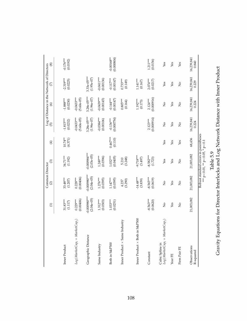
Com

mon

Dir

ecto

rLo

gof

Dis

tanc

ein

the

Net

wor

kof

Dir

ecto

rs(1

)(2

)(3

)(4

)(5

)(6

)(7

)(8

)

Inne

rPr

oduc

t31

.83*

**33

.48*

**34

.71*

**10

.74*

*-1

.815

***

-1.8

88**

*-2

.319

***

-0.1

76**

*(1

.117

)(1

.207

)(1

.192

)(4

.371

)(0

.023

2)(0

.023

0)(0

.022

5)(0

.019

2)

Log(

Mar

ketC

api×

Mar

ketC

apj)

0.22

9***

0.22

8***

-0.0

433*

**-0

.043

3***

(0.0

0406

)(0

.004

06)

(5.6

0e-0

5)(5

.60e

-05)

Geo

grap

hic

Dis

tanc

e-0

.000

980*

**-0

.000

980*

**-0

.000

984*

**3.

28e-

05**

*3.

28e-

05**

*3.

33e-

05**

*(2

.04e

-05)

(2.0

4e-0

5)(2

.03e

-05)

(1.9

6e-0

7)(1

.96e

-07)

(1.9

5e-0

7)

Sam

eIn

dust

ry1.

312*

**1.

276*

**1.

249*

**-0

.038

4***

-0.0

439*

**-0

.041

1***

(0.0

303)

(0.0

395)

(0.0

396)

(0.0

0106

)(0

.001

45)

(0.0

0136

)

Both

inS&

P500

1.03

3***

1.14

7***

1.03

2***

0.46

7***

-0.1

36**

*-0

.144

***

-0.1

17**

*-0

.001

68**

(0.0

251)

(0.0

395)

(0.0

405)

(0.1

10)

(0.0

0075

4)(0

.001

47)

(0.0

0147

)(0

.000

804)

Inne

rPr

oduc

t×Sa

me

Indu

stry

4.23

75.

210

0.80

5***

0.73

3***

(3.2

90)

(3.2

48)

(0.1

64)

(0.1

49)

Inne

rPr

oduc

t×Bo

thin

S&P5

00-1

4.48

***

-9.7

18**

*1.

192*

**1.

141*

**(3

.839

)(3

.497

)(0

.173

)(0

.167

)

Con

stan

t-8

.563

***

-8.5

65**

*-8

.582

***

2.12

3***

2.12

4***

2.07

4***

1.21

1***

(0.0

620)

(0.0

619)

(1.7

23)

(0.0

0091

4)(0

.000

916)

(0.0

217)

(0.0

156)

Cub

icSp

line

inLo

g(M

arke

tCap

i×

Mar

ketC

apj)

No

No

Yes

Yes

No

No

Yes

Yes

Year

FEYe

sYe

sYe

sYe

sYe

sYe

sYe

sYe

s

Firm

Pair

FEN

oN

oN

oYe

sN

oN

oN

oYe

s

Obs

erva

tion

s21

,003

,082

21,0

03,0

8221

,003

,082

68,4

3616

,239

,841

16,2

39,8

4116

,239

,841

16,2

39,8

41R

-squ

ared

0.22

40.

224

0.22

90.

840

Rob

usts

tand

ard

erro

rsin

pare

nthe

ses

***

p<

0.01

,**

p<

0.05

,*p<

0.1

Tabl

e5.

9G

ravi

tyEq

uati

ons

for

Dir

ecto

rIn

terl

ocks

and

Log

Net

wor

kD

ista

nce

wit

hIn

ner

Prod

uct

108

Figure 5.1Network of Interlocking Directorships for US Firms: 2010

Source: Corporate Library, Thomson Reuters, and author’s calculations.

109

100 101 10210−4

10−3

10−2

10−1

100

Degree k

Frac

tion

of fi

rms

P k hav

ing

degr

ee k

or g

reat

er

20012011

Figure 5.2Degree Distribution for the Network of Interlocking Directors: 2001 and 2010

110

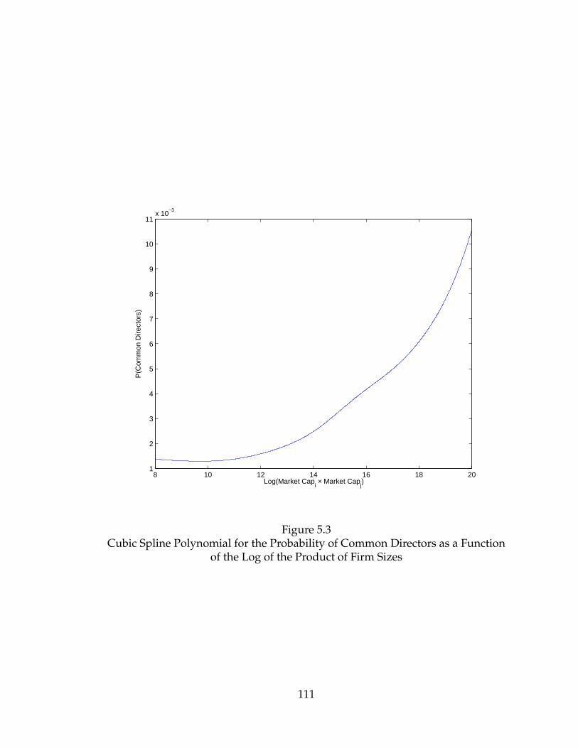
8 10 12 14 16 18 201

2

3

4

5

6

7

8

9

10

11x 10

−3

Log(Market Capi × Market Cap

j)

P(C

omm

on D

irect

ors)

Figure 5.3Cubic Spline Polynomial for the Probability of Common Directors as a Function

of the Log of the Product of Firm Sizes

111

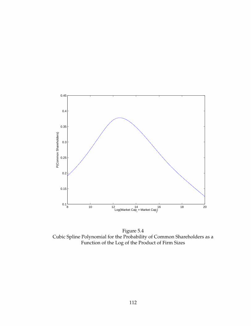
8 10 12 14 16 18 200.1

0.15

0.2

0.25

0.3

0.35

0.4

0.45


j)

P(C

omm

on S

hare

hold

ers)

Figure 5.4Cubic Spline Polynomial for the Probability of Common Shareholders as a

Function of the Log of the Product of Firm Sizes

112

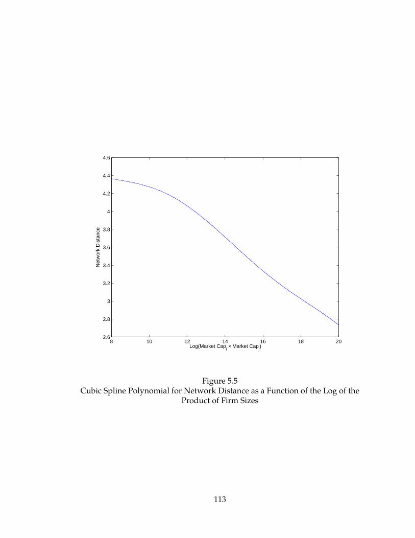
8 10 12 14 16 18 202.6

2.8

3

3.2

3.4

3.6

3.8

4

4.2

4.4

4.6


j)

Net

wor

k D

ista

nce

Figure 5.5Cubic Spline Polynomial for Network Distance as a Function of the Log of the

Product of Firm Sizes

113

8 10 12 14 16 18 200.03

0.032

0.034

0.036

0.038

0.04

0.042

0.044

0.046

0.048


j)

Max

imin

Figure 5.6Cubic Spline Polynomial for Maximin as a Function of the Log of the Product of

Firm Sizes

114

8 10 12 14 16 18 200.06

0.07

0.08

0.09

0.1

0.11

0.12

0.13

0.14

0.15


j)

Sum

of M

ins

Figure 5.7Cubic Spline Polynomial for the Sum of Mins as a Function of the Log of the


115

8 10 12 14 16 18 203.5

4

4.5

5

5.5

6

6.5

7

7.5

8x 10

−3


j)

Inne

r P

rodu

ct

Figure 5.8Cubic Spline Polynomial for the Inner Product as a Function of the Log of the


116

2001 2002 2003 2004 2005 2006 2007 2008 2009 20101

1.5

2

2.5

3

3.5

4

4.5

5x 10

−3

Year

P(C

omm

on D

irect

ors)

RawControlling for Size and Other Covariates

Figure 5.9Evolution of the Probability of Director Interlocks

117

Chapter 6

Shareholder Networks and Market

Power

6.1 Introduction

In this chapter, study empirically of the relationship between common ownership

and market power. I start by showing the evolution of markups for a sample of

US and Canadian firms over time. Second, I document a positive correlation be-

tween a company’s markup and the fraction of firms in its industry with which

it has common shareholders. To study the relationship in more depth, I show the

results of structure-conduct-performance (SCP) regressions at the industry level,

with average markups as the dependent variable and measures of common own-

ership, plus controls, as an explanatory variables. The main result is that the

industry-level density of shareholder networks is positively associated with av-

erage industry markups. I then study the joint dynamics of markups and common

ownership measures using a Panel Vector Autoregression. The analysis shows that


118

markups. Average markups, on the other hand, do not have predictive power for

industry-level density.

The structure-conduct-performace literature attempted, for several decades

and with limited success, to find a relationship between concentration measures

and measures of market power. For a classic survey, see Schmalensee (1989),

which highlights the problems of the endogeneity of market structure, and sig-

nificant issues related to the measurement of markups. The empirical literature

on common ownership and market power is scarce. An interesting contribution

is the work of Parker and Roller (1997).They study the effect of cross-ownership

and multimarket contact in the mobile telephone industry. In the early 1980s

in the United States, the Federal Communications Commission created local

duopolies in which two firms were allowed to operate in strictly defined product

and geographic markets. Since before the market structure was monopolistic,

this provides an interesting opportunity to study the effect of changes in market

structure on prices. They find that both cross-ownership and multimarket contact

led to collusive behavior.

6.2 Data

I use two datasets: Compustat fundamentals quarterly North America for account-

ing data on American and Canadian firms, and Thomson Reuters institutional

holdings for ownership data. I focus on the period 2000Q2-2010Q4. There are

180,355 firm-quarter observations that have data on both accounting and institu-

tional ownership, with a total of 7277 firms. I drop from the sample industries

that have only one firm in the data. After this, the sample has 179,201 firm-quarter

observations. Then, I drop observations with earnings before taxes higher than

revenues, observations with negative markups (the calculation of markups is ex-

119

plained in detail in the next paragraph), and observations with zero revenues.

Thus, I end up with a sample size of 172,247 firm-quarter observations. The av-

erage number of firms in the sample per quarter is 4,006, with a minimum of 3,648

firms and a maximum of 4,267. There are 249 industries at the 3-digit SIC level rep-

resented in the sample. Because of the presence of extreme outliers, I windsorize

the markup at the 1st and 99th percentiles.

The first step in the empirical analysis is to construct the adjacency matrix for

a network of firms linked by the common ownership generated by institutional

investors. I consider two firms as being connected in the shareholder network if

there is at least one shareholder owning at least 5 percent in each firm. Once we

have constructed this matrix, we can then calculate the degree of each firm at each

point in time, that is, the number of connections with other firms in the network.

We can also calculate the density of the network. The formula for the density of a

network, given its adjacency matrix Y, is

Density =∑n

i=1 ∑j<i yij

n(n− 1)/2,

where n is the number of nodes in the network and yij is equal to 1 if firm i and

firmj are connected, and zero otherwise (by convention, a firm is not considered to

be connected to itself, and thus the adjacency matrix has zeros in its diagonal).

In addition to a firm’s overall degree, we will find it useful to consider its

within-industry degree, that is, the number of connections that it has with other

firms in the same industry. Because the number of firms in the sample varies across

time, we will normalize both the overall degree and the within-industry degree by

dividing them by the number of other firms in the sample, and the number of other

firms in the sample that are in the same industry, respectively. These normalized

120

measures represent the percentage of possible connections, rather than the raw

number of connections.

We will also find it useful to consider, in addition to the density of the overall

network, the density of the subnetwork for each industry. To do this, we take the

firms in only one industry and consider the network formed by those firms and

their connections.

Figure 4.1 shows a plot of the network for a random sample of 400 companies

in 2010Q4, representing roughly 10% of the companies in the network. There are

several clusters generated by a few institutional investors which have ownership

stakes of more than 5 percent in a large number of companies. The two largest

clusters, in the center of the network plot, are generated by BlackRock and Fidelity.

The firms with the highest numbers of connections are those that belong to both of

these two large clusters.

To calculate markups, I use data on revenues and earnings before taxes. The

difference between these two is a measure of total cost. Markups are then calcu-

lated as

Markupit =Revenueit

Costit.

As is well known, this measure of markups has several drawbacks. The first is

that it uses average cost rather than marginal cost, and is thus a measure of the

average markup, rather than the markup at the margin, which is the one that the

theory refers to. Second, it fails to capture all of the user cost of capital, since,

although it includes interest expenses, does not take into account the opportunity

cost of equity capital. Its main advantage is that it is possible to calculate it using

standard accounting data, which is readily available for a large number of firms.

However, it is important to keep in mind that markups are measured with error.

Table 6.1 shows summary statistics for assets, markups, whether a firm has

a large shareholder, the number of connections of the firms in the sample in the

121

shareholder network, the normalized number of connections (that is, the number

of connections divided by the number of other firms in the sample for that quarter),

and the normalized number of connections with other firms in the same industry

(that is, the number of connections with other firms in the industry divided by the

number of other firms in the industry for that quarter).

Figure 6.1 shows the evolution over time of the density of the shareholder net-

work for the economy as a whole, and of the average density of the industry sub-

networks. The points for 2010Q1 and 2010Q2 have been interpolated, because

the lack of BlackRock data for those quarters distorted the measures substantially.

Consistent with the evidence in Chapter 4, industry subnetworks are denser on

average than the overall network. This means that the probability that two firms

will have a common shareholder is higher if they are in the same industry. A

difference-in-means test shows that the difference is statistically significant. Also

consistent with the evidence described in that chapter, the density of shareholder

networks, both at the industry level and overall, increased substantially between

2000 and 2010. Both the overall density and the average within-industry density

have approximately tripled over that period.

Figure 6.2 shows the evolution of the average and median markups over time.

Markups are procyclical, consistent with the evidence presented by Nekarda and

Ramey (2010). There is also an upward trend, although it is slight compared to the

large cyclical movements.

Figure 6.3 shows that there is a positive relationship between markups and

firm size, measured as the logarithm of assets. I first average markups and log

assets over time for each firm. Then, I divide the firms into deciles by size, and

calculate the average markup for each decile. Interestingly, average markups are

below one for the bottom 5 deciles, and above for the top 5. Figure 6.4 shows

that smaller firms on average also have a higher fraction of periods with negative

122

income (before taxes), and less periods with observations, presumably because of

a higher probability of exit.

Figure 6.5 shows the result of a similar exercise, but dividing the firms by the

number of within-industry connections instead of log assets. First, I separate the

2334 (out of 7277) firms that have no connections within their industry in any pe-

riod, and calculate their average markup. Then, I divide the rest of the firms into

quintiles according to the fraction of possible within-industry connections, and cal-

culate the average markup for each group. There is a strong positive correlation

between within-industry connections and markups. If we control for log assets, by

using the residuals from a regression of markups on log assets (and adding the av-

erage markup to the residuals) instead of raw markups, the correlation in smaller,

but still significant. Interestingly, there is a positive jump in markups when going

from the second to the third quintile of connections. Figure 6.6 shows that more

connected firms are on average less likely to have negative profits (before taxes).

Figure 6.7 shows that more connected firms have more periods with observations,

presumably because their exit probability is lower. In all cases, the relationships

described hold when controlling for assets, with the exception that the fraction

of periods with negative income is lower for firms with no connections than for

connected firms in the lowest two quintiles.

6.3 Regression Analysis

Table 6.2 shows the results of structure-conduct-performance regressions of av-

erage industry markups on the density of industry common ownership subnet-

works, average overall degree (normalized) of firms in the industry, and controls.

123

The basic specification is

Markupit = β0 + β1Densityit + β2Average Degreeit + Controlsit + εit.

Control variables include the average log of assets of the firms in the indus-

try, the Herfindahl index, calculated using the share of revenues of the firms in

the dataset, the number of firms in the industry (within the dataset), and the frac-

tion of firms in the industry that have a large institutional shareholder, that is, an

institutional investor owning more than 5 percent of the firm.

The first specification is a cross-sectional regression for a balanced panel of 210

industries, using time averages of all variables. The second specification is esti-

mated using a Fama-MacBeth two-step procedure. The third specification uses the

data without aggregating over time, and includes quarterly dummies to correct

for temporal variation in markups. The fourth specification adds lagged markups,

which helps control for omitted variable bias. The fifth specification includes in-

dustry fixed effects, which helps control for omitted variables that are constant

over the whole period. The last specification includes both lagged markups and

fixed effects.1

In all specifications, we see a positive relation between markups and within-

industry shareholder density. We also see a negative relation between overall con-

nectivity of firms in the industry (that is, including connections with firms in other

industries) and markups. The partial correlation between within-industry den-

sity and markups is statistically significant in all specifications except the one with

fixed effects but no lagged markups. Note that the lack of statistical significance

in the case of fixed effects without lagged markups is driven by higher standard

errors, rather than a lower coefficient. This suggests that a) some of the effect is

1While in general including both lagged dependent variables and fixed effects leads to inconsis-tent estimates, given the large number of periods (41 quarters) and the relatively low value of theautoregressive parameter, the bias in this case should be small.

124

coming from the between-industry variation, and b) some of the omitted variables

are time-varying. Fixed effects estimates are known to exacerbate the bias due

to measurement error. The measurement error problem could be substantial in

this case, since a) we do not observe non-institutional owners, and b) using a 5%

threshold will count some firms as connected when they are not, and viceversa.

The positive relationship between average industry markups and within-

industry shareholder network density is consistent with a partial horizontal

integration interpretation. That is, industries where firms are more likely to share

the same owners, according to the theory, should have higher markups all else

equal. The negative relationship between average industry markups and average

overall connectivity in terms of common ownership is consistent with a partial

vertical integration interpretation. When firms become vertically integrated, the

double marginalization problem is solved. Thus, standard industrial organization

models predict that markups when firms are vertically integrated should be lower

than when they are independent (see Tirole, 1994, chap. 4).

Industries with larger firms in terms of assets tend to have higher markups.

Ownership concentration, measured as the fraction of firms in the industry with

large shareholders (more than 5% ownership) has a statistically significant effect

only in two specifications. In the Fama-MacBeth regression, the effect is positive

and significant at 5%. In the specification with fixed effects and lagged markups,

the effect is negative and significant at 10%. The Herfindahl index has no statisti-

cally significant effect, except for a negative effect, significant at 10%, in the speci-

fication with fixed effects and lagged markups. The inverse of the number of firms

in the industry does not have a statistically significant effect on markups. The lack

of a clear relationship between measures of concentration and markups should not

be too surprising, given the failure of the structure-conduct-performance literature

125

to find a strong relationship between these measures of concentration and market

power.

6.4 Panel Vector Autoregression Analysis

In this section, I study the dynamics of industry-level density and average

markups. To do this, I use a Panel Vector Autoregression (Panel VAR). The main

econometric issue in the estimation of Panel VARs is the endogeneity problem

that arises when including both fixed effects and lagged dependent variables.

The endogeneity bias, however, goes to zero as the length of the panel goes to

infinity. Since the panel used in this chapter is relatively long (i.e., 42 periods), the

bias introduced by having fixed effects and lagged dependent variables should be

relatively small.2

I estimate the following reduced form specification:

yi,t = B1(L)yi,t−1 + B2xi,t + εi,t,

where yi,t is a vector of endogenous variables that includes average industry

markups, industry density, average industry degree, average log assets for the

firms in the industry, the fraction of firms in the industry with a blockholder at

5%, and the Herfindahl index. As exogenous variables, xi,t, I include quarterly

dummies, and also industry fixed effects in some specifications.

To obtain error bands for impulse responses, I use the same Bayesian procedure

used in time-series VARs, described in detail in Sims and Zha (1999), with a flat

prior. When applying these methods in a panel setting, it is necessary to introduce

breaks to separate the observations for different industries.

2For a discussion and a proposed estimator, see Holtz-Eakin et al. (1988). Barcellos (2010) uses aPanel VAR to study the dynamics of immigration and wages in the United States.

126

To be able to obtain impulse responses, I impose contemporaneous restrictions

with the following order of the variables: mean log assets, Herfindahl, average

markup, fraction of firms with a large shareholder, average degree, and density.

Thus, all variables, and in particular, the markup, can affect density contempora-

neously. On the other hand, this ordering assumes that density has a zero contem-

poraneous effect on all the other variables.

Table 6.3 shows the results of a one-lag panel vector autoregression, with quar-

terly dummies and without fixed effects. We see that markups do not help to

explain the density of shareholder networks. Shareholder network density, on the

other hand, has a positive and highly significant effect on markups. Consistent

with the results from the regression analysis, average degree has a statistically sig-

nificant negative effect. This is confirmed by the impulse response analysis, shown

in Figures 6.8 and 6.9.

Table 6.4 shows the results of a one-lag panel vector autoregression, with quar-

terly dummies and fixed effects. The results are qualitatively similar as in the anal-

ysis without fixed effects. The effect of common ownership measures on markups

is smaller, but still statistically significant. The impulse response posterior densi-

ties are shown in Figures 6.10 and 6.11.

6.5 Summary

In this chatper, I studied the relationship between networks of common owner-

ship and markups at the industry level. The main result is that the industry-

level density of shareholder networks is positively associated with average indus-

try markups. A dynamic analysis using Panel Vector Autoregressions shows that


127

markups, but average markups do not have predictive power for industry-level

density.

128

Obs. Mean Median 90th Pct. 10th Pct. Std. Dev.

Assets 172247 6844.6 384.7 8279 24.5 53692.5

Markup 172247 1.04 1.05 1.35 0.59 0.41

Large shareholder 172247 0.71 1.0 1.0 0.0 0.46

Degree (number of connexions) 172247 326.5 88 986 0 424.9

Percentage of possible connectionswith other firms in the economy 172247 7.7% 2.1% 23.1% 0.0% 0.10

Percentage of possible connectionswith other firms in the same industry 172247 10.2% 1.2% 32.2% 0.0% 0.15


This table shows summary statistics for the variables used in the analysis of shareholder networksand markups. The data is quarterly, and goes from 2000Q2 to 2010Q4. Assets are in millions ofdollars. The calculation of markups is described in section 7.1. The percentage of connectionswith other firms in the economy is the total number of connections for a given firm in a givenperiod divided by the number of firms in that period minus one. The percentage of connectionswith other firms in the same industry is calculated as the number of connections with firms in thesame 3-digit SIC industry for a given firm in a given period divided by the number of firms inthat industry in that period minus one. Two firms are considered connected if there is at least oneshareholder holding at least 5% in both firms. Large shareholder is an indicator variable, equal toone if a company has a shareholder with at least 5% of the shares and zero otherwise. Outliers arewindsorized at the 1st and 99th percentile by quarter.

129

Dependent Variable: Average Markup(1) (2) (3) (4) (5) (6)

Density 0.246*** 0.0641*** 0.0668** 0.0246** 0.0240 0.0213**(0.0819) (0.00756) (0.0277) (0.0107) (0.0155) (0.0107)

Average Degree -1.210*** -0.430*** -0.403*** -0.125*** -0.206** -0.142**(0.347) (0.0559) (0.124) (0.0477) (0.0863) (0.0568)

Average Log Assets 0.0312*** 0.0329*** 0.0325*** 0.0112*** 0.0455*** 0.0322***(0.00561) (0.00143) (0.00458) (0.00193) (0.00926) (0.00674)

1 / (Number of Firms) -0.0354 -0.00669 0.000470 0.0104 0.120 0.124(0.0811) (0.0160) (0.0525) (0.0196) (0.111) (0.0802)

Herfindahl 0.0489 0.00725 0.00365 -0.00634 -0.0739 -0.0671*(0.0493) (0.00800) (0.0353) (0.0129) (0.0519) (0.0398)

Fraction w/Large Shareholders 0.0943 0.0176** 0.0153 0.00240 -0.0221 -0.0232*(0.0631) (0.00837) (0.0248) (0.0107) (0.0180) (0.0138)

Markupt−1 0.679*** 0.403***(0.0314) (0.0293)

Constant 0.855*** 0.867*** 0.879*** 0.271*** 0.817*** 0.452***(0.0640) (0.0104) (0.0417) (0.0324) (0.0519) (0.0439)

Quarterly Dummies N/A N/A Yes Yes Yes YesIndustry Fixed Effects N/A N/A Yes YesObservations 210 9,524 9,524 9,008 9,524 9,008Number of Industries 210 249 249 246 249 246R-squared 0.196 0.129 0.141 0.544 0.122 0.275

Table 6.2Average Markups and Measures of Common Ownership

This table shows industry-level regression results with average industry markups (before taxes) asthe dependent variable and measures of common ownership as explanatory variables. Standarderrors are in parentheses. Specification (1) is a cross-sectional regression of averages over timeusing a balanced panel, with White heteroskedasticity-robust standard errors. Specification (2) isestimated using the two-step procedure of Fama-MacBeth. The standard errors in specifications (3)to (6) are clustered at the industry level. *** p<0.01, ** p<0.05, * p<0.1.

130

(1) (2) (3) (4) (5) (6)Markup Density Degree Log Assets Herfindahl Large Sh.

Markupt−1 0.685*** 0.000689 -0.00255 -0.0391* 0.00726 0.0159*(0.00770) (0.00723) (0.00165) (0.0233) (0.00568) (0.00861)

Densityt−1 0.0267*** 0.798*** 0.00143 0.0402 0.00195 0.00684(0.00826) (0.00776) (0.00177) (0.0250) (0.00609) (0.00924)

Degreet−1 -0.155*** 0.240*** 0.903*** -0.175* -0.00837 0.240***(0.0346) (0.0325) (0.00740) (0.105) (0.0255) (0.0387)

Log Assetst−1 0.00843*** -6.69e-05 -0.000107 0.976*** -0.000865 -0.00109(0.000832) (0.000781) (0.000178) (0.00252) (0.000613) (0.000930)

Herfindahlt−1 0.00674 -0.00957** -0.00350*** 0.00319 0.948*** -0.0223***(0.00458) (0.00430) (0.000978) (0.0139) (0.00337) (0.00512)

Large Sh.t−1 0.00456 0.0145** 0.00390*** -0.0664*** -0.0172*** 0.798***(0.00638) (0.00598) (0.00136) (0.0193) (0.00470) (0.00713)

Constant 0.277*** 0.00150 0.00758*** 0.203*** 0.0201** 0.127***(0.0113) (0.0106) (0.00241) (0.0342) (0.00832) (0.0126)

Quarterly Dummies Yes Yes Yes Yes Yes YesObservations 9,008 9,008 9,008 9,008 9,008 9,008R-squared 0.540 0.705 0.835 0.951 0.899 0.704

Table 6.3Vector Autoregression Results

This table shows regression results for a vector autoregression with one lag, without industry fixedeffects. Standard errors in parentheses. *** p<0.01, ** p<0.05, * p<0.1.

131

(1) (2) (3) (4) (5) (6)Markup Density Degree Log Assets Herfindahl Large Sh.

Markupt−1 0.416*** -0.0144 -0.00384* -0.0252 0.000910 0.00444(0.00979) (0.00967) (0.00220) (0.0302) (0.00705) (0.0112)

Densityt−1 0.0217** 0.664*** -0.00226 0.0159 -0.00179 -0.00260(0.00970) (0.00958) (0.00218) (0.0299) (0.00699) (0.0111)

Degreet−1 -0.142*** 0.252*** 0.806*** 0.125 -0.0124 0.105**(0.0405) (0.0400) (0.00911) (0.125) (0.0292) (0.0463)

Log Assetst−1 0.0105*** 0.00219 0.00208*** 0.711*** -0.00506*** 0.0135***(0.00259) (0.00255) (0.000581) (0.00797) (0.00186) (0.00296)

Herfindahlt−1 0.0242** -0.0511*** -0.0155*** -0.0384 0.568*** -0.130***(0.0123) (0.0121) (0.00276) (0.0378) (0.00884) (0.0140)

Large Sh.t−1 -0.00440 -0.0127 -0.00911*** 0.0450* -0.0342*** 0.592***(0.00814) (0.00804) (0.00183) (0.0251) (0.00587) (0.00931)

Constant 0.555*** 0.0657*** 0.0462*** 2.015*** 0.239*** 0.267***(0.0203) (0.0201) (0.00457) (0.0626) (0.0146) (0.0232)

Quarterly Dummies Yes Yes Yes Yes Yes YesIndustry Fixed Effects Yes Yes Yes Yes Yes YesObservations 9,008 9,008 9,008 9,008 9,008 9,008R-squared 0.617 0.728 0.848 0.958 0.920 0.742

Table 6.4Vector Autoregression Results

This table shows regression results for a vector autoregression with one lag, with industry fixedeffects. Standard errors in parentheses. *** p<0.01, ** p<0.05, * p<0.1.

132

0%

2%

4%

6%

8%

10%

12%

14%

16%

18%

2000 2001 2002 2003 2004 2005 2006 2007 2008 2009 2010

Density (Whole Network) Average Within-‐Industry Density

Figure 6.1Shareholder Network Density over Time

This figure shows the evolution of the density of the network of firms generated by common in-stitutional shareholders with ownership stakes of at least 5% in a pair of firms, and of the averagedensity of the industry subnetworks. Industries are defined at the 3-digit SIC level. The valuesfor 2010Q1 and 2010Q2 are interpolated (linearly) because ownership data for BlackRock, the topinstitution in terms of number of blockholdings in 2010, was not available for those quarters.

133

0.9

0.95

1

1.05

1.1

1.15

2000 2001 2002 2003 2004 2005 2006 2007 2008 2009 2010

Average Markup Median Markup

Figure 6.2Average and Median Markups over Time

This figure shows the evolution over time of the average and median markup for the firms inthe sample. Markups are calculated as total accounting revenues (before taxes) divided by totalaccounting costs (before taxes).

134

0.6

0.7

0.8

0.9

1

1.1

1.2

1st Decile

2nd Decile

3rd Decile

4th Decile

5th Decile

6th Decile

7th Decile

8th Decile

9th Decile

10th Decile

Figure 6.3Average Markup, by Decile of Log Assets

This figure shows the average markup in the cross section of firms for each decile of firm size,measured as log assets. The markup of each firm and its log assets are averaged over all the periodsfor which it has observations.

135

0

0.1

0.2

0.3

0.4

0.5

0.6

0.7

0.8

0.9

1st Decile

2nd Decile

3rd Decile

4th Decile

5th Decile

6th Decile

7th Decile

8th Decile

9th Decile

10th Decile

(a) Average Fraction of Periods with Negative Income (BeforeTaxes)

10

15

20

25

30

35

1st Decile

2nd Decile

3rd Decile

4th Decile

5th Decile

6th Decile

7th Decile

8th Decile

9th Decile

10th Decile

(b) Average Number of Periods with Observations

Figure 6.4Average Fraction of Periods with Negative Income (Before Taxes) and Average

Number of Periods with Observations, by Decile of Log Assets

This figure shows the average fraction of periods with negative income before taxes and the averagefraction of periods for which a firm has observations, in the cross section of firms for each decile offirm size, measured as log assets.

136

0.85

0.9

0.95

1

1.05

1.1

No Connec.ons 1st Quin.le 2nd Quin.le 3rd Quin.le 4th Quin.le 5th Quin.le

(a) No Controls

0.95

0.96

0.97

0.98

0.99

1

1.01

No Connec0ons 1st Quin0le 2nd Quin0le 3rd Quin0le 4th Quin0le 5th Quin0le

(b) Controlling for Log Assets

Figure 6.5Average Markup, by Quintile of Within-Industry Degree

This figure shows the average markup in the cross section of firms for each quintile of within-industry normalized degree, after separating the observations with zero within-industry connec-tions. Within-industry normalized degree is calculated as the number of connections that a com-pany has with other firms in the same 3-digit SIC industry divided by the number of other firms inthe industry (i.e. the number of possible connections). The markup of each firm and its log assetsare averaged over all the periods for which it has observations.

137

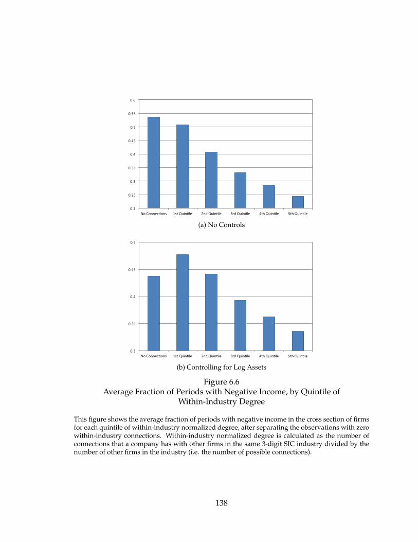
0.2

0.25

0.3

0.35

0.4

0.45

0.5

0.55

0.6

No Connec/ons 1st Quin/le 2nd Quin/le 3rd Quin/le 4th Quin/le 5th Quin/le

(a) No Controls

0.3

0.35

0.4

0.45

0.5

No Connec-ons 1st Quin-le 2nd Quin-le 3rd Quin-le 4th Quin-le 5th Quin-le


Figure 6.6Average Fraction of Periods with Negative Income, by Quintile of

Within-Industry Degree

This figure shows the average fraction of periods with negative income in the cross section of firmsfor each quintile of within-industry normalized degree, after separating the observations with zerowithin-industry connections. Within-industry normalized degree is calculated as the number ofconnections that a company has with other firms in the same 3-digit SIC industry divided by thenumber of other firms in the industry (i.e. the number of possible connections).

138

10

15

20

25

30

35


(a) No Controls

10

15

20

25

30



Figure 6.7Average Number of Periods with Observations, by Quintile of Within-Industry

Degree

This figure shows the average number of periods with observations in the cross section of firmsfor each quintile of within-industry normalized degree, after separating the observations with zerowithin-industry connections. Within-industry normalized degree is calculated as the number ofconnections that a company has with other firms in the same 3-digit SIC industry divided by thenumber of other firms in the industry (i.e. the number of possible connections).

139

0 5 10 15

−6

−4

−2

0

2

4

6

x 10−3Shock to Large Sh.

Mar

kup

0 5 10 15

−6

−4

−2

0

2

4

6

x 10−3Shock to Degree

0 5 10 15

−6

−4

−2

0

2

4

6

x 10−3Shock to Density

Figure 6.8Response of the Average Industry Markup to Shocks to Ownership Structure

Variables

This figure shows the posterior density, in a Panel VAR model, of the response of average markupsto shocks to the fraction of firms with large shareholders in the industry, the average overall degreeof the firms in the industry, and the industry’s shareholder subnetwork density. The endogenousvariables in the VAR are average log assets, the Herfindahl index, average markups, the fractionof firms with a large shareholder, the average degree, and the density of the industry network.Quarterly dummies are treated as exogenous variables. In each figure, the x axis indicates numberof quarters after shock. The graph shows bands from 5%, up to 95%, in intervals of 5%.

140

0 2 4 6 8 10 12 14 16 18−5

0

5

10x 10

−3Shock to Markup

Larg

e S

h.

0 2 4 6 8 10 12 14 16 18−2

−1.5

−1

−0.5

0

0.5

1x 10

−3

Deg

ree

0 2 4 6 8 10 12 14 16 18−5

−4

−3

−2

−1

0

1

2

3

4

5x 10

−3

Den

sity

Figure 6.9Response of Ownership Structure Variables to Shocks to Average Industry

Markups

This figure shows the posterior density, in a Panel VAR model, of the response of the fraction offirms with large shareholders in the industry, the average overall degree of the firms in the industry,and the industry’s shareholder subnetwork density to shocks to average markups. The endogenousvariables in the VAR are average log assets, the Herfindahl index, average markups, the fractionof firms with a large shareholder, the average degree, and the density of the industry network.Quarterly dummies are treated as exogenous variables. In each figure, the x axis indicates numberof quarters after shock. The graph shows bands from 5%, up to 95%, in intervals of 5%.

141

0 5 10 15

−4

−3

−2

−1

0

1

2

3

4x 10−3

Shock to Large Sh.

Mar

kup

0 5 10 15

−4

−3

−2

−1

0

1

2

3

4x 10−3

Shock to Degree

0 5 10 15

−4

−3

−2

−1

0

1

2

3

4x 10−3

Shock to Density

Figure 6.10Response of the Average Industry Markup to Shocks to Ownership Structure

Variables (including Industry Fixed Effects)

This figure shows the posterior density, in a Panel VAR model, of the response of average markupsto shocks to the fraction of firms with large shareholders in the industry, the average overall degreeof the firms in the industry, and the industry’s shareholder subnetwork density. The endogenousvariables in the VAR are average log assets, the Herfindahl index, average markups, the fractionof firms with a large shareholder, the average degree, and the density of the industry network.Quarterly dummies and industry fixed effects are treated as exogenous variables. In each figure,the x axis indicates number of quarters after shock. The graph shows bands from 5%, up to 95%, inintervals of 5%.

142

0 2 4 6 8 10 12 14 16 18−5

−4

−3

−2

−1

0

1

2

3

4

5x 10

−3Shock to Markup

Larg

e S

h.

0 2 4 6 8 10 12 14 16 18−2

−1.5

−1

−0.5

0

0.5

1x 10

−3

Deg

ree

0 2 4 6 8 10 12 14 16 18−5

−4

−3

−2

−1

0

1

2

3

4

5x 10

−3

Den

sity

Figure 6.11Response of Ownership Structure Variables to Shocks to Average Industry

Markups (including Industry Fixed Effects)

This figure shows the posterior density, in a Panel VAR model, of the response of the fraction offirms with large shareholders in the industry, the average overall degree of the firms in the industry,and the industry’s shareholder subnetwork density to shocks to average markups. The endogenousvariables in the VAR are average log assets, the Herfindahl index, average markups, the fractionof firms with a large shareholder, the average degree, and the density of the industry network.Quarterly dummies and industry fixed effects are treated as exogenous variables. In each figure,the x axis indicates number of quarters after shock. The graph shows bands from 5%, up to 95%, inintervals of 5%.

143

Chapter 7

Conclusion: Adjusting the Herfindahl

Index for Portfolio Diversification?

In this dissertation, I developed a theory of oligopoly with shareholder voting. I

also showed evidence that common ownership among publicly traded US firms

has increased in the last decade, and that empirical measures of common owner-

ship are predictors of (a) a higher probability of interlocking directorships at the

firm-pair level and (b) higher markups at the level of the industry.

I have argued that society faces a trilemma. Portfolio diversification, maximiza-

tion of shareholder value by managers, and competition are considered desirable

objectives. However, it is not possible to completely attain the three. Balancing

these objectives presents us with a complex policy problem.

One possible way to proceed would be to adjust the Herfindahl index for port-

folio diversification. This could be useful to detect industries with high levels of

concentration, taking into account not just market shares but also the links of com-

mon ownership between the firms. In the following section, I show how to adjust

the Herfindahl index for portfolio diversification based on the model of oligopoly

with shareholder voting.

144

7.1 A Herfindahl Index Adjusted for Common Own-

ership

In this section I derive an analogue to the Herfindahl index of market concentra-

tion that takes into account the links of common ownership between the firms in

the industry. Consider a Cournot model of oligopoly with shareholder voting,

with homogeneous goods and heterogeneous costs, in which all shareholders are

equally activist, uniformly across firms. From Chapter 2, we know that the first

order condition for firm i is

∫g∈G

θgi

[θ

gi (α− 2βqi − βq−i −mi) + ∑

j 6=iθ

gj (−βqj)

]dg = 0.

This can be rewritten as

α− 2βqi − βq−i −mi = ∑j 6=i

λijβqj,

where

λij ≡

∫g∈G θ

gi θ

gj dg∫

g∈G (θgi )

2dg.

This expression, in turn, can be rewritten in terms of the markup, market

shares, and the inverse price elasticity of demand, as follows:

P−mi

P=

si

η+

∑j 6=i sjλij

η,

where si = qi/Q is the market share of firm i and 1/η = −P′(Q)Q/P is the inverse

price elasticity of demand.

145

The average Lerner index weighted by market shares is

P−∑Ni=1 simi

P=

∑Ni=1 s2

iη

+∑N

i=1 ∑j 6=i sisjλij

η.

When firms are separately owned, we are in the classic Cournot case, and the

average markup is proportional to the Herfindahl H = ∑Ni=1 s2

i . However, when

firms have common shareholders, this is no longer the case. However, the above

expression suggests a formula for an index H that adjusts the Herfindahl in the

presence of common ownership links:

H = H +N

∑i=1

∑j 6=i

sisjλij.

This index can also be expressed more concisely as follows:

H =N

∑i=1

N

∑j=1

sisjλij,

since λii = 1. It is straightforward to show that H is between zero and one, and is

always higher than the Herfindahl.

We can summarize these results in the following

Theorem 7. Consider a Cournot model of oligopoly with shareholder voting with (a) linear

demands, (b) homogeneous goods, (c) heterogeneous constant marginal costs, and (d) the

same level of activism for all shareholders and all firms. In this model, the average markup

(weighted by the market shares) is proportional to the adjusted Herfindahl index

H = H +N

∑i=1

∑j 6=i

sisjλij,

where H = ∑Ni=1 s2

i is the unadjusted Herfindahl index.

146

Note that all the information in the portfolios necessary to calculate the index

is summarized by the N×N sufficient statistics λij. We can think of these statistics

as defining a weighted and directed network connecting the firms in the industry

through links of common ownership. The adjusted Herfindahl H is can be thought

of a weighted average of the links in the network of common ownership, where

the weights are the products of the market shares of each pair of nodes (note that

∑Ni=1 ∑N

j=1 sisj = 1).

7.1.1 An Example

Consider an industry with five symmetric firms, each with a market share of .2.

The Herfindahl index for the industry is equal to .2. The U.S. Department of Jus-

tice and FTC Horizontal Merger Guidelines consider industries with a Herfind-

ahl above .15 and below .25 to be moderately concentrated, and industries with a

Herfindahl higher than .25 to be highly concentrated. Thus, this industry would

be considered moderately concentrated, but not highly concentrated.

If the firms in the industry have completely separate owners, the adjusted

Herfindahl is also equal to .2. However, suppose that the firms have five own-

ers. Each owner owns 80% of one of the firms, and in addition has a 5% stake

in each of the other firms in the industry (another way to put it is that each owner

has 75% of one firm, plus a diversified portfolio that has 5% of the whole industry).

The adjusted Herfindahl is .31. Thus, adjusting for common ownership would put

the industry in the highly concentrated category. Note that a merger between two

firms in the industry would increase the adjusted Herfindahl by a lower amount

than what the same merger would increase the unadjusted Herfindahl, since the

firms in the industry are already partially merged.

147

7.2 A Model-Based Measure of Common Ownership

at the Firm-Pair Level

In empirical studies of shareholder networks, the links are usually derived in an

ad hoc way based on a threshold percentage for ownership stakes. For example,

two firms are considered connected if there is a shareholder with ownership stakes

of at least 5% in both, and not connected otherwise. While this measure is useful

for its simplicity, it would be useful to have a measure of common ownership that

did not depend on an arbitrary threshold, and did not have a discontinuity at the

threshold. The analysis of the previous section suggests that the normalized inner

product λij is a good candidate for this measure. The interpretation of λij as a

measure of the common ownership between a pair of firms applies in contexts

much more general than the Cournot model with homogeneous goods.

Consider a model of oligopoly with shareholder voting with risk-neutral share-

holders. In equilibrium, firms maximize a weighted average of shareholder utili-

ties. The problem of firm i is

maxpi

∫g∈G

θgi E

[N

∑j=1

θgj πj(pj, p−j)

]dg.

This can be rewritten as

maxpi

(∫g∈G

(θgi )

2dg)

Eπi + ∑j 6=i

(∫g∈G

θgi θ

gj dg)

Eπj,

which is equivalent to maximizing

maxpi

Eπi + ∑j 6=i

λijEπj.

148

Thus, the normalized inner product λij can be interpreted as the weight of the

expected profits of firm j in the decision problem of firm i.

This is a directed measure of common ownership, such that λij 6= λji. For some

applications it will be useful to define an undirected measure λij as the geometric

mean of the two directed measures:

λij =√

λijλji =

∫g∈G θ

gi θ

gj dg√(∫

g∈G (θgi )

2dg) (∫

g∈G (θgj )

2dg) .

This normalized inner product is an uncentered correlation coefficient for the own-

ership structures of firm i and firm j.

The use of this measure in practice could be problematic if there is no data for

all the owners of the firms in the pair. For example, if we take only shareholders

with stakes of 1% or more, and ignore shareholders with smaller shares, then the

calculated measure would be the same for a pair of firms with one shareholder

having 1% in both firms (and all other shareholders having less than 1% in either)

as for a pair of firms with one shareholder having 10% in both firms (and all other

shareholders having less than 1% in either). Thus, one should be careful when

applying this measure.

7.3 Possible Directions for Future Research

While theoretically appealing, the practical application of the Herfindahl index

adjusted for portfolio diversification poses significant challenges. First, it requires

relatively complete data on the ownership of all the firms in the industry. Sec-

ond, the measure taken literally does not take into account agency problems, and

therefore the weight of the links does not put a penalty on lack of concentration

of ownership. In practice, however, this could be important: for the same level of

149

the normalized inner products, if the ownership of the firms is more concentrated,

collusion could potentially be easier, because the agency problem would be less in-

tense. One possible way to proceed would be to consider management as having

weight in the maximization problem of the firm, and defining what the objective

of the management is. For example, one could assume that managers care only

about the profits of the firm that they manage.

Another possible avenue for further research would be to relax the assump-

tion of atomistic shareholders. Large institutional shareholders play an important

role in the ownership of publicly traded firms in the United States and in other

countries. When shareholders are large, this opens the door to the possibility of

strategic considerations in portfolio allocation. That is, when choosing their port-

folios in the first stage, shareholders would take into account that they can have

a significant impact in the outcome of the voting equilibrium in the second stage.

Another issue that is related to the presence of large shareholders is the possibility

of hostile takeovers, which are not possible in a model with atomistic shareholders,

unless they can borrow non-atomistic amounts.

From an empirical point of view, there is also much work to be done. It would

be of interest to study the relationship between market power and the Herfind-

ahl adjusted for portfolio diversication. As already noted, this implies significant

challenges from the point of view of both data availability and theory.

In this dissertation, I have focused on firms in the United States. However,

portfolio diversification includes cross-country diversification, and institutional

investors hold stocks in more than one country. Studying the evolution of port-

folio diversification and networks of common ownership at an international level

would be a natural direction for further research.

150

Bibliography

D. Acemoglu. An Introduction to Modern Economic Growth. Princeton UniversityPress, 2009.

A. Agrawal and G.N. Mandelker. Large shareholders and the monitoring of man-agers: The case of antitakeover charter amendments. Journal of Financial andQuantitative Analysis, 25(02):143–161, 1990. ISSN 0022-1090.

D.S. Ahn and S. Oliveros. Combinatorial Voting. 2010.

A. Alesina and H. Rosenthal. Partisan politics, divided government, and the economy.Cambridge Univ Pr, 1995. ISBN 0521436206.

A. Alesina and H. Rosenthal. A theory of divided government. Econometrica: Jour-nal of the Econometric Society, 64(6):1311–1341, 1996. ISSN 0012-9682.

F. Allen, M.K.F. Chui, and A. Maddaloni. Financial systems in europe, the usa, andasia. Oxford Review of Economic Policy, 20(4):490–508, 2004.

K.J. Arrow. A difficulty in the concept of social welfare. The Journal of PoliticalEconomy, 58(4):328–346, 1950. ISSN 0022-3808.

K.J. Arrow. Collected papers of Kenneth J. Arrow: Social choice and justice. Belknap Pr,1983. ISBN 0674137604.

S.H. Barcellos. The dynamics of immigration and wages. Working Paper, 2010.

M. Becht and J.B. DeLong. Why has there been so little block holding in america?,2005.

M. Becht and A. Roell. Blockholdings in europe: An international comparison.European Economic Review, 43(4):1049–1056, 1999.

A.A. Berle and G.C. Means. The modern corporation and private property. 1940.

M. Bertrand and S. Mullainathan. Are CEOS Rewarded for Luck? The Ones with-out Principals Are*. Quarterly Journal of Economics, 116(3):901–932, 2001. ISSN0033-5533.

J.E. Bethel, J.P. Liebeskind, and T. Opler. Block share purchases and corporateperformance. The Journal of Finance, 53(2):605–634, 1998. ISSN 1540-6261.

151

B. Blonigen and C. O’Fallon. Foreign firms and local communities. Technical re-port, National Bureau of Economic Research, 2011.

J.A. Brander and T.R. Lewis. Oligopoly and financial structure: The limited liabilityeffect. The American Economic Review, 76(5):956–970, 1986. ISSN 0002-8282.

Y. Cai and M. Sevilir. Board connections and m&a transactions. Journal of FinancialEconomics, 2011.

G. Cestone. Corporate financing and product market competition: An overview.Giornale degli Economisti e Annali di Economia, 58(2):269–300, 1999. ISSN 0017-0097.

V.V. Chari, L.E. Jones, and R. Marimon. The economics of split-ticket voting inrepresentative democracies. The American Economic Review, 87(5):957–976, 1997.ISSN 0002-8282.

P.J. Coughlin. Probabilistic voting theory. Cambridge Univ Pr, 1992. ISBN0521360528.

S. Cukurova. Interlocking directors and target selection in mergers and acquisi-tions. 2011.

H. DeAngelo. Competition and unanimity. The American Economic Review, 71(1):18–27, 1981.

J.B. DeLong. Did J.P. Morgan’s men add value. Inside the Business Enterprise, pages205–36, 1991.

P.M. DeMarzo. Majority voting and corporate control: the rule of the dominantshareholder. The Review of Economic Studies, 60(3):713–734, 1993. ISSN 0034-6527.

P.A. Diamond. The role of a stock market in a general equilibrium model withtechnological uncertainty. The American Economic Review, 57(4):759–776, 1967.ISSN 0002-8282.

E. Dierker, H. Dierker, and B. Grodal. Nonexistence of constrained efficient equi-libria when markets are incomplete. Econometrica, 70(3):1245–1251, 2002. ISSN1468-0262.

A. Dixit. A model of duopoly suggesting a theory of entry barriers. The Bell Journalof Economics, 10(1):20–32, 1979. ISSN 0361-915X.

G.W. Domhoff. Who rules america? 1967.

J.H. Dreze. (Uncertainty and) the firm in general equilibrium theory. The EconomicJournal, 95:1–20, 1985. ISSN 0013-0133.

D. Duffie and W. Shafer. Equilibrium and the Role of the Firm in Incomplete Mar-kets, Research Paper no. 915, Graduate School of Business, 1986.

152

S. Ekern and R. Wilson. On the theory of the firm in an economy with incompletemarkets. Bell Journal of Economics, 5(1):171–180, 1974.

C. Fershtman and K.L. Judd. Equilibrium incentives in oligopoly. The AmericanEconomic Review, 77(5):927–940, 1987. ISSN 0002-8282.

R. Foellmi and J. Zweimuller. Inequality, market power, and product diversity.Economics Letters, 82(1):139–145, 2004.

M. Friedman. The social responsibility of business is to increase its profits. NewYork Times Magazine, pages 122–126, 1970.

S.L. Gillan and L.T. Starks. The Evolution of Shareholder Activism in the UnitedStates*. Journal of Applied Corporate Finance, 19(1):55–73, 2007. ISSN 1745-6622.

P.A. Gompers and A. Metrick. Institutional investors and equity prices*. QuarterlyJournal of Economics, 116(1):229–259, 2001.

R.H. Gordon. Do publicly traded corporations act in the public interest? Technicalreport, National Bureau of Economic Research, 1990.

S.J. Grossman and J.E. Stiglitz. On value maximization and alternative objectivesof the firm. Journal of Finance, pages 389–402, 1977.

J. Hackner. A Note on Price and Quantity Competition in DifferentiatedOligopolies. Journal of Economic Theory, 93(2):233–239, 2000. ISSN 0022-0531.

R.G. Hansen and J.R. Lott. Externalities and corporate objectives in a world withdiversified shareholder/consumers. Journal of Financial and Quantitative Analysis,31(1), 1996.

J. Harford, D. Jenter, and K. Li. Institutional cross-holdings and their effect onacquisition decisions. Journal of Financial Economics, 99(1):27–39, 2011.

O. Hart and J. Moore. The governance of exchanges: Members’ cooperatives ver-sus outside ownership. Oxford Review of Economic Policy, 12(4):53–69, 1996.

J.C. Hartzell and L.T. Starks. Institutional investors and executive compensation.The Journal of Finance, 58(6):2351–2374, 2003. ISSN 1540-6261.

D. Holtz-Eakin, W. Newey, and H.S. Rosen. Estimating vector autoregressions withpanel data. Econometrica: Journal of the Econometric Society, pages 1371–1395, 1988.

T. Ito. The Japanese Economy, volume 10. The MIT Press, 1992.

M.C. Jensen and J.B. Long. Corporate investment under uncertainty and paretooptimality in the capital markets. The Bell Journal of Economics and ManagementScience, pages 151–174, 1972.

153

J.K. Kang and A. Shivdasani. Firm performance, corporate governance, and topexecutive turnover in Japan. Journal of Financial Economics, 38(1):29–58, 1995.ISSN 0304-405X.

S.N. Kaplan and B.A. Minton. Appointments of outsiders to Japanese boards: De-terminants and implications for managers. Journal of Financial Economics, 36(2):225–258, 1994. ISSN 0304-405X.

S.N. Kaplan and B.A. Minton. How has ceo turnover changed? International Reviewof Finance, 2008.

D. Kelsey and F. Milne. The existence of equilibrium in incomplete markets and theobjective function of the firm. Journal of Mathematical Economics, 25(2):229–245,1996. ISSN 0304-4068.

D. Kelsey and F. Milne. Imperfect competition and corporate governance. Journalof Public Economic Theory, 10(6):1115–1141, 2008. ISSN 1467-9779.

D.W. Kim. Interlocking ownership in the korean chaebol. Corporate Governance: AnInternational Review, 11(2):132–142, 2003.

A.F. Ledvina and R. Sircar. Bertrand and Cournot competition under asymmetriccosts: number of active firms in equilibrium. 2010.

L. Makowski. Competition and unanimity revisited. The American Economic Review,73(3):329–339, 1983.

Harry Markowitz. Portfolio selection. The Journal of Finance, 7(1):pp. 77–91, 1952.ISSN 00221082. URL http://www.jstor.org/stable/2975974.

G. Matvos and M. Ostrovsky. Cross-ownership, returns, and voting in mergers.Journal of Financial Economics, 89(3):391–403, 2008.

F. Milne. Corporate Investment and Finance Theory in Competitive Equilibrium*.Economic Record, 50(4):511–533, 1974. ISSN 1475-4932.

F. Milne. The firm’s objective function as a collective choice problem. Public Choice,37(3):473–486, 1981. ISSN 0048-5829.

M.S. Mizruchi. What do interlocks do? an analysis, critique, and assessment ofresearch on interlocking directorates. Annual review of sociology, pages 271–298,1996.

G.D. Myles. Public economics. Cambridge Univ Pr, 1995.

J.P. Neary. The road less travelled: Oligopoly and competition policy in generalequilibrium. 2002.

J.P. Neary. International trade in general oligopolistic equilibrium. University Col-lege Dublin, mimeo, 2009.

154

C.J. Nekarda and V.A. Ramey. The cyclical behavior of the price-cost markup.University of California, San Diego (July), 2010.

P.M. Parker and L.H. Roller. Collusive conduct in duopolies: multimarket contactand cross-ownership in the mobile telephone industry. The RAND Journal ofEconomics, pages 304–322, 1997.

M. Poitevin. Collusion and the Banking Structure of a Duopoly. Canadian Journalof Economics, 22(2):263–277, 1989. ISSN 0008-4085.

R. Radner. A note on unanimity of stockholders’ preferences among alternativeproduction plans: a reformulation of the ekern-wilson model. The Bell Journal ofEconomics and Management Science, pages 181–184, 1974.

T. Renstrom and E. Yalcin. Endogenous firm objectives. Journal of public economictheory., 5(1):67–94, 2003. ISSN 1097-3923.

R. J. Reynolds and B. R. Snapp. The competitive effects of partial equity interestsand joint ventures. International Journal of Industrial Organization, 4:141–153, 1986.

M.J. Roe. Strong managers, weak owners: The political roots of American corporate fi-nance. Princeton Univ Pr, 1996.

R. Schmalensee. Inter-industry studies of structure and performance. ch. 16 in r.schmalensee and r. willig (eds.): Handbook of industrial organization, vol. 2,1989.

C.A. Sims and T. Zha. Error bands for impulse responses. Econometrica, 67(5):1113–1155, 1999.

N. Singh and X. Vives. Price and quantity competition in a differentiated duopoly.The RAND Journal of Economics, 15(4):546–554, 1984. ISSN 0741-6261.

T.E. Stuart and S. Yim. Board interlocks and the propensity to be targeted in privateequity transactions. Journal of Financial Economics, 97(1):174–189, 2010.

J. Tirole. The theory of industrial organization. MIT press, 1994.

155

implicit collusion through portfolio diversification

Documents