Working Paper/Document de travail2007-47

Implications of Asymmetry Risk for Portfolio Analysis and Asset Pricing

by Fousseni Chabi-Yo, Dietmar Leisen, and Eric Renault

www.bankofcanada.ca

Bank of Canada Working Paper 2007-47

August 2007

Implications of Asymmetry Risk forPortfolio Analysis and Asset Pricing

by

Fousseni Chabi-Yo 1, Dietmar Leisen 2, and Eric Renault 3

1Financial Markets DepartmentBank of Canada

Ottawa, Ontario, Canada K1A 0G9

2Faculty of Law and EconomicsJohannes Gutenberg-Universität Mainz

3Department of EconomicsUniversity of North Carolina at Chapel Hill

Chapel Hill, NC 27599-3305and CIRANO, CIREQ, Montréal

renault@email.unc.edu

Bank of Canada working papers are theoretical or empirical works-in-progress on subjects ineconomics and finance. The views expressed in this paper are those of the authors.

No responsibility for them should be attributed to the Bank of Canada.

ISSN 1701-9397 © 2007 Bank of Canada

ii

Acknowledgements

We thank Scott Hendry, Kenneth Judd and Wally Speckert for very helpful conversations. We

thank seminar participants at the EC2 Conference in Rotterdam for helpful comments.

iii

Abstract

Asymmetric shocks are common in markets; securities’ payoffs are not normally distributed and

exhibit skewness. This paper studies the portfolio holdings of heterogeneous agents with

preferences over mean, variance and skewness, and derives equilibrium prices. A three funds

separation theorem holds, adding a skewness portfolio to the market portfolio; the pricing kernel

depends linearly only on the market return and its squared value. Our analysis extends Harvey and

Siddique’s (2000) conditional mean-variance-skewness asset pricing model to non-vanishing risk-

neutral market variance. The empirical relevance of this extension is documented in the context of

the asymmetric GARCH-in-mean model of Bekaert and Liu (2004).

JEL classification: C52, D58, G11, G12Bank classification: Financial markets; Market structure and pricing

Résumé

Les chocs asymétriques sont des phénomènes courants sur les marchés. La distribution des

rendements des actifs financiers ne suit pas une loi normale et est asymétrique. Les auteurs

étudient la composition du portefeuille d’agents hétérogènes qui ont des préférences à l’égard de

la moyenne, de la variance et de l’asymétrie de la distribution des rendements, et calculent les prix

d’équilibre des actifs. Ils démontrent la validité d’un théorème de séparation à trois portefeuilles,

selon lequel les agents détiennent un portefeuille dont les rendements sont répartis de façon

asymétrique en plus du portefeuille standard du marché; le facteur d’actualisation stochastique ne

dépend linéairement que du rendement du marché et du carré de celui-ci. Les auteurs étendent le

modèle d’évaluation des actifs financiers à trois moments conditionnels (moyenne, variance et

asymétrie) de Harvey et Siddique (2000) pour y inclure une variance du rendement du marché

neutre à l’égard du risque et toujours supérieure à zéro. Ils testent empiriquement la pertinence de

cette extension au moyen du modèle GARCH-M asymétrique de Bekaert et Liu (2004).

Classification JEL : C52, D58, G11, G12Classification de la Banque : Marchés financiers; Structure de marché et fixation des prix

1. Introduction

Asymmetric shocks are common in markets; securities�payo¤s are not normally distributed and

exhibit skewness. Moreover, even when primary assets have symmetric payo¤s, typical derivatives

assets display a high degree of skewness. The important contribution of Harvey and Siddique

(2000) renewed interest in the compensation for skewness risks and led to an active literature1.

This paper revisits the pricing implications of Stochastic Discount Factors (henceforth SDF) which

are quadratic in the market return, and links the price of skewness risk to derivatives and to risk-

neutral variance. We particularly stress the importance of a conditional viewpoint for estimation of

the skewness premium. Furthermore, while the literature is largely based on ad-hoc extensions of

the CAPM where the squared market return is a priced factor (in addition to the market return),

this paper provides a theoretical foundation for this practice.

Samuelson (1970) studied the limit of portfolio holdings under in�nitesimal risk2 and concluded

that mean-variance analysis largely characterizes the optimal portfolio problem even when the

decision maker has a general concave Von Neumann-Morgenstern utility function and asset returns

are not normally distributed. In the presence of �small�risks it is necessary to study also the slope

of portfolio holdings in the neighborhood of in�nitesimal risk. This paper extends Samuelson�s

analysis of �nancial decision making to this slope and thereby introduces skewness risk into the

analysis; we derive agents�portfolio holdings and the equilibrium allocation under mean-variance-

skewness risk.

In the �rst part of the paper, we characterize agents�portfolio holdings using risk-tolerance

and a term we call skew-tolerance which contains the third derivative of agents�utility functions.

Risk-tolerance captures the mean-variance trade-o¤and skew-tolerance the mean-variance-skewness

trade-o¤. Using appropriately de�ned �average� risk-tolerance and �average� skew-tolerance we

show that such an �average�agent sets price. We prove a separation theorem in which heteroge-

neous agents�holdings are composed of two funds: the market portfolio and a new portfolio we

call the skewness portfolio. Among all portfolios, the skewness portfolio is the portfolio with a

return �closest� to that of the squared market return. Agents�holdings of the market portfolio

2

are proportional to individual risk-tolerance; holdings of the skewness portfolio are proportional to

risk-tolerance multiplied by the di¤erence between the individual agent�s skew-tolerance and that

of the �average�agent. Although the return from the skewness portfolio di¤ers from the squared

market return, it remains true that any risk is compensated only through its relationship with the

market, either through standard market beta or through market coskewness which is akin to beta

with respect to the squared market return. In this respect, one may say that both idiosyncratic

variance and idiosyncratic skewness are not compensated in equilibrium.

In the second part of the paper, we study extensively the pricing implications of an SDF

which is quadratic in the market return. Although motivated by our extension of Samuelson�s

small risk analysis, this part of our study is valid under very general settings and is compared to

previous literature on the pricing of skewness risks. Along these lines, we revisit beta pricing under

skewness as it has been considered previously by Kraus and Litzenberger (1976), Ingersoll (1987),

and Harvey and Siddique (2000), among others. We also relate skewness pricing to important terms

in derivatives pricing: to risk neutral variance, which has been studied extensively by Rosenberg

(2000), and to the price of volatility contracts, studied by Bakshi and Madan (2000).

Our paper makes the following three contributions. First, we provide a rigorous foundation

for the use of SDF that are quadratic in the market return. Most empirical studies looked at

skewness extensions of the CAPM which add the squared market return as a factor. Those authors

that justify this extension base their proofs on assumed separation and aggregation results or on

ad-hoc truncation of a Taylor-series expansion for the representative agent utility function at the

third-order term, see, e.g., Kraus and Litzenberger (1976), Barone-Adesi (1985), Dittmar (2002).

The insight of Samuelson (1970) was that the use of mean-variance analysis does not have to be

based on truncated Taylor-series expansions: limits with vanishing risk justify such an analysis

as an approximation3. Our extension of Samuelson�s analysis to skewness risk permits a rigorous

analysis of separation and aggregation: we prove that simple market separation does not hold but

that, somewhat surprisingly, the SDF depends locally on the squared market return. The skewness

portfolio, projection of the squared market return on primitive assets, plays the role of an additional

3

mutual fund.

It is important to stress that this aggregation result is not a trivial consequence of standard

complete market arguments. Actually, when only considering linear portfolios in primitive asset

returns, markets are not complete in terms of hedging squared market return. It turns out that, due

to a preference for positive skewness, tracking the squared market return is of interest for investors.

While higher order small noise expansions are beyond the scope of this paper, it can be shown (see

Chabi-Yo, Ghysels and Renault (2007)) that, when taking into account investors�preferences for

low kurtosis, our asset pricing model depends on the cross-sectional variance of investors� skew-

tolerances. Therefore, heterogeneity of investor preferences matters for equilibrium asset pricing,

precisely because nonlinear payo¤s are relevant risks for investors which are not perfectly hedged.

Second, we study extensively the pricing implications of SDF that are quadratic in the market

return. We shed more light on beta pricing relationships proposed by Harvey and Siddique (2000)

and show that they correspond to a limit case of a zero-risk neutral variance of the market. We

put forward a more general beta pricing relationship, which explicitly depends on the price of the

squared return on the market portfolio, or equivalently, on the market risk neutral variance. This

opens the door to more extensive studies of the skewness premium based on derivatives prices.

Finally, we add to the literature which aims at identifying the skewness premium. The statis-

tical identi�cation of a signi�cantly positive skewness premium is generally considered a di¢ cult

task, see, e.g. Barone-Adesi, Urga and Gagliardini (2004). We provide some empirical evidence

which suggests that such premia show up in a more manifest way when they are considered with

a conditional point of view, as it has been in Harvey and Siddique (2000). Our evidence is docu-

mented from simulated data on the GARCH factor model with in-mean e¤ects using the parameter

estimates of Bekaert and Liu(2004). Moreover, our simulations also suggest that neglecting the

market risk neutral variance � as it has been, e.g., in Harvey and Siddique (2000) � leads to a

severe underestimation of the skewness premium which may go so far as to invert its sign.

The remainder of the paper is organized as follows. The next section discusses portfolio choice

and asset pricing in the context of in�nitesimal risks. Section 3 studies quadratic pricing kernels

4

in the conditional setup of Hansen and Richard (1987). Section 4 makes an empirical assessment

of the order of magnitude of the various e¤ects put forward in Section 3. Section 5 concludes the

paper. Lengthy proofs are postponed to the appendix.

2. Static Portfolio Analysis in Terms of Mean, Variance and Skew-ness

Samuelson (1970) argues that, for risks that are in�nitely small, optimal shares of wealth invested in

each security coincide with those of a mean-variance optimizing agent. However Samuelson (1970)

also derives a more general approximation theorem about higher order approximations: to further

characterize the way the optimal shares vary locally in the direction of any risk, that is their �rst

derivatives at the limit point of zero risk, one needs to push the Taylor expansion of the utility

function one step further. Carrying this out will lead us to a mean-variance-skewness approach.

We start here from a slight generalization of Samuelson�s result. Following closely his exposition,

let us denote by Ri, the (gross) return from investing $1 in risky security i = 1; :::; n. The random

vector R = (Ri)1�i�n de�nes the joint probability distribution of interest, which is speci�ed by the

following decomposition:

Ri (�) = Rf + �2ai (�) + �Yi: (1)

Here, ai (�), i = 1; :::; n, are positive functions of � and Rf is the gross return on the riskless

(safe) security. The � parameter characterizes the scale of risk and is crucial for our analysis.

In this section, we are interested in approximations in the neighborhood of � = 0. The small

noise expansion (1) provides a convenient framework to analyze portfolio holdings and resulting

equilibrium allocations for a given random vector Y = (Yi)1�i�n with

E [Y ] = 0; and V ar (Y ) = �;

where � is a given symmetric and positive de�nite matrix4. For future reference, we denote by

�k = EhY Y ?Yk

i

5

the matrix of covariances between Yk and cross-products YiYj , i; j = 1; :::; n. Typically, asymmetry

in the joint distribution of returns means that at least some matrices �k, k = 1; :::; n are not zero.

In equation (1), the term �2ai (�) has the interpretation of the risk premium. Samuelson (1970)

restricts the function ai (�) to constants; under this assumption risk premia are proportional to the

squared scale of risk; we relax this restriction throughout since it would prevent us from analyzing

the price of skewness in equilibrium. Throughout, we refer to a (�) = (ai (�))i=1;:::;n as the vector

of risk premia.

2.1 The individual investor problem

We consider an investor with Von Neumann-Morgenstern preferences, i.e. she derives utility from

date 1 wealth according to the expectation over some increasing and concave function u evaluated

over date 1 wealth; for given risk-level � she then seeks to determine portfolio holdings (!i)1�i�n 2

Rn that maximize her expected utility

max(!i)1�i�n2Rn

Eu

Rf +

nXi=1

!i � (Ri (�)�Rf )!: (2)

Note that, for the sake of notational simplicity, we normalized the initial wealth invested to one.

The solution of this program is denoted by (!i (�))1�i�n and depends on the given scale of risk

�. The question we ask is then the following: to what extent does a Taylor approximation of u

allow us to understand the local behaviour of the shares !i (�) in the neighborhood of the zero risk

� = 0? Put di¤erently, we want to characterize for i = 1; :::; n the quantities:

!i (0) = lim��!0+

!i (�) and !0i (0) = lim

��!0+!0i (�) : (3)

Samuelson (1970) stresses that a third order Taylor expansion of u is needed to do the job. We

slightly extend his result by showing that it remains valid even though the functions ai (�) are

not assumed to be constant in our analysis. For this purpose let us consider a third order Taylor

expansion of u in the neighborhood of the safe return Rf :

u� (W ) = u (Rf ) + u0 (Rf ) (W �Rf ) +

u00 (Rf )

2!(W �Rf )2 +

u000 (Rf )

3!(W �Rf )3 : (4)

6

Let us denote by (!�i (�))1�i�n the solution of the approximated problem, i.e. (!�i (�))1�i�n 2 Rn

describes the holdings of an agent with utility function u�:

max(!�i )1�i�n

Eu�

Rf +

nXi=1

!�i � (Ri (�)�Rf )!

(5)

For i = 1; :::; n the terms !�i (0) and !�0i (0) are de�ned similar to (3) as continuity extensions. We

state that Taylor expansions give tangency equivalences.

Theorem 2.1 Under suitable smoothness and concavity assumptions, the solution to the general

problem (2) is related asymptotically to that of the 3-moment problem by the tangency equivalences:

!i (0) = !�i (0) and !0i (0) = !�0i (0) for all i = 1; :::; n:

The intuition behind this theorem is that in the limit case � 0:

1. The optimal shares of wealth invested !i (0), i = 1; :::; n depend on its �rst two derivatives

u0 (Rf ) and u00 (Rf ). Thus, a second order Taylor expansion of u, that is a mean-variance

approach, provides a correct characterization of these shares.

2. The �rst derivatives with respect to �, !0i (0), i = 1; :::; n of optimal shares depend on the

utility function u only through its �rst three derivatives u0(Rf ), u

00(Rf ) and u

000(Rf ). Thus,

a third order Taylor expansion of u, that is a mean-variance-skewness approach, does the job.

In the following we will analyze portfolio holdings. For future reference, in this subsection we

denote by

� = � u0(Rf )

u00 (Rf )and � =

�2

2

u000(Rf )

u0 (Rf )(6)

the risk-tolerance coe¢ cient and the skew-tolerance coe¢ cient of the agent.

Of course, the risk-tolerance coe¢ cient � is assumed to be positive, to capture risk aversion,

while the skew-tolerance coe¢ cient � is non negative, following the literature on preferences for

higher order moments (Dittmar (2002), Harvey and Siddique (2000)). This assumption may also

be justi�ed by reference to prudence (Kimball (1990)).

7

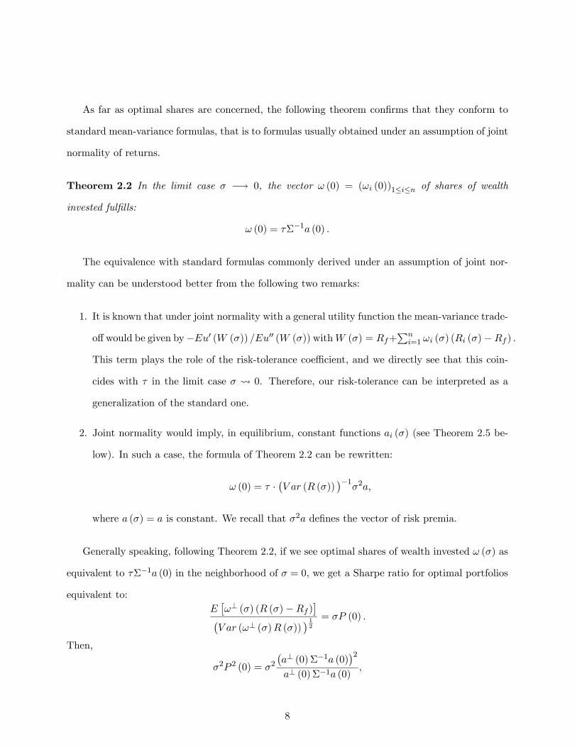
As far as optimal shares are concerned, the following theorem con�rms that they conform to

standard mean-variance formulas, that is to formulas usually obtained under an assumption of joint

normality of returns.

Theorem 2.2 In the limit case � �! 0, the vector ! (0) = (!i (0))1�i�n of shares of wealth

invested ful�lls:

! (0) = ���1a (0) :

The equivalence with standard formulas commonly derived under an assumption of joint nor-

mality can be understood better from the following two remarks:

1. It is known that under joint normality with a general utility function the mean-variance trade-

o¤would be given by�Eu0 (W (�)) =Eu00 (W (�)) withW (�) = Rf+Pni=1 !i (�) (Ri (�)�Rf ) :

This term plays the role of the risk-tolerance coe¢ cient, and we directly see that this coin-

cides with � in the limit case � 0. Therefore, our risk-tolerance can be interpreted as a

generalization of the standard one.

2. Joint normality would imply, in equilibrium, constant functions ai (�) (see Theorem 2.5 be-

low). In such a case, the formula of Theorem 2.2 can be rewritten:

! (0) = � ��V ar (R (�))

��1�2a;

where a (�) = a is constant. We recall that �2a de�nes the vector of risk premia.

Generally speaking, following Theorem 2.2, if we see optimal shares of wealth invested ! (�) as

equivalent to ���1a (0) in the neighborhood of � = 0, we get a Sharpe ratio for optimal portfolios

equivalent to:E�!? (�) (R (�)�Rf )

��V ar (!? (�)R (�))

� 12

= �P (0) :

Then,

�2P 2 (0) = �2�a? (0)��1a (0)

�2a? (0)��1a (0)

;

8

so that

P (0) =ha? (0)��1a (0)

i 12: (7)

This denotes, by unit of scaling risk �, the potential performance of the set R of returns as in

traditional mean variance analysis (see e.g. Jobson and Korkie (1982)). Of course, the above

analysis neglects the variation in equilibrium of the risk premium functions a (�). We are going to

see in Theorem 2.5 below that these functions will not be constant, even locally in the neighborhood

of � = 0, as soon as the joint asset-return probability-distribution features some asymmetries.

These asymmetries will actually play a double role in the local behaviour of optimal shares

of wealth invested. First, preferences for skewness would increase, ceteris paribus, asset demands

in the direction of positive skewness. Second, market equilibrium induced variations in the risk

premium potentially erase this e¤ect. To see this, let us de�ne the coskewness of asset k in portfolio

! as:

De�nition 2.3 The coskewness of asset k in portfolio ! is:

ck (!) =1

�

Cov�Rk;

�!? (R� ER)

�2�V ar (!? (R� ER)) : (8)

Note that coskewness does not depend on the scale of risk �. We will see below that this notion

of coskewness is tightly related to a measure put forward by Kraus and Litzenberger (1976) (see

also Ingersoll (1987), p. 100).

The vector c (!) = (ck (!))1�k�n represents a multivariate notion of skewness. We can show

that investors prefer positive skewness, component-wise. This assertion is justi�ed by the fact that

the average

nXk=1

!kck (!) =1

�

Eh�!? (R� ER)

�3iV ar

�!? (R� ER)

�=

1

�Skew

�!? � (R� ER)

���V ar

�!? � (R� ER)

�� 12

is positive if and only if the portfolio return is positively skewed. We then get the following result:

9

Theorem 2.4 The slope !0 (0) of the vector ! (0) of optimal shares of wealth invested in the neigh-

borhood of � = 0 is given by:

!0 (0) = ���1 ��a0 (0) + �P 2 (0) c

�;

where a0 (0) = (a0i (0))1�i�n is the vector of marginal risk premia and c = c (! (0)) = c����1a (0)

�.

In other words, up to variations a0(0) of risk premia in equilibrium, a positive coskewness of

asset k will have a positive e¤ect on the demand for this asset with respect to common mean-

variance formulas. This positive e¤ect will be all the more pronounced when the skew-tolerance

coe¢ cient � is large.

Individual preferences for positive skewness will increase, ceteris paribus, the equilibrium price

of assets with positively skewed returns. This e¤ect will appear in the equilibrium value a0(0) of

risk premium slopes in the neighborhood of � = 0 (see below).

2.2 Equilibrium Allocations and Prices

Let us consider asset markets for risky assets i = 1; 2; :::; n on which S agents can trade. For agent

s = 1; :::; S, we denote !s (0) =�!0si (0)

�1�i�n

her holdings in each of these assets; her preferences

are characterized by a Von Neumann-Morgenstern utility function us and associated preference

coe¢ cients:

� s = �u0s (Rf )

u00s (Rf )and �s =

�2s2

u000s (Rf )

u0s (Rf ): (9)

From theorems 2.2 and 2.4 we get that:

!s (0) = ��1� sa (0) , !

0s (0) = � s�

�1ha0(0) + �2s (0)P

2 (0) c (! (0))i: (10)

Note that these formulas correspond to the case where each of the S agents would get a unit of

wealth to invest. Generalization to more realistic, non-uniform distributions of initial wealth would

be easy to state, but this would merely complicate the notation without adding any insight to

the analysis of this paper. Therefore, the only heterogeneity considered in this paper is about

preferences.

10

An average investor will be de�ned by average preferences, which are average risk tolerance �

and average skew tolerance �, such that:

� =1

S

SXs=1

� s; and � =

SPs=1

�s� s

SPs=1

� s

: (11)

Note that the average skew tolerance is computed with weights proportional to risk tolerance, so

that:SXs=1

� s (�s � �) = 0: (12)

We consider that the net supply of each risky asset i = 1; :::; n is exogenous and independent of

the scale of risk �. Then, Taylor expansions of individual portfolios�shares must ful�ll the market

clearing conditions:

SXs=1

!s (0) = S!; andSXs=1

!0s (0) = 0: (13)

where ! is the portfolio that would be selected by an average investor with characteristics (� ; �).

Jointly with individual asset demands (10), market clearing conditions (13) determine the Taylor

expansion of the risk premium function a (�) in equilibrium:

Theorem 2.5 In the limit case � 0, the equilibrium risk premium vector a (�) is such that the

average portfolio ! is optimal for the average investor: ! = ���1a (0), that is

a (0) =1

��!:

Its slope in the neighborhood of zero is given by:

a0k (0) = ��P 2 (0) ck (!) for k = 1; :::;K:

Theorem 2.5 must be interpreted as a new asset pricing model. While approximating risk premia

by their limit values ai (0) would clearly lead to the Sharpe-Lintner CAPM, approximating them

by higher order expansions ai (0) + �a0i (0) results in a new mean-variance-skewness asset pricing

model. To see this, let us assume for notational simplicity that the total supply of the risk-free

11

asset is zero. Then, the average portfolio ! has a unit price (since we have assumed that each

investor has a unit wealth) and RM = !?R denotes the market return. Then

� =Cov (R;RM )

V ar (RM )=

�!

!?�!(14)

denotes the vector of market betas of the n assets.

Thus, not surprisingly, the �rst part of Theorem 2.5 states that the limit value a (0) of the vector

of equilibrium risk premium is proportional to the vector of market betas, with a proportionality

coe¢ cient V ar(RM )� = ��2P 2 (0), which is itself increasing with market risk and market risk aversion.

The new contribution of Theorem 2.5 is encapsulated in the value

a0k (0) = ��P 2 (0) ck (!) : (15)

It states that insofar as utility functions are not quadratic (� 6= 0), asset k exhibits a positive

skewness risk premium a0k (0) when its coskewness ck (!) in the market portfolio is negative. As

already explained, an asset k should be preferred, ceteris paribus, when it contributes positively to

the market skewness. By contrast, when it contributes negatively, investors have to be compensated

for that e¤ect. This compensation is captured through a risk premium function a (�) which is not

constant in the neighborhood of � = 0, by contrast with Samuelson�s (1970) analysis.

Individual asset demands in equilibrium are then determined from the results of Section 2.1,

when plugging in the equilibrium values of a (0) and a0 (0):

Theorem 2.6 In equilibrium, in the limit case � 0, the optimal shares of wealth invested !s (�)

of agents s = 1; :::; S are characterized by:

!s (0) =� s�!; and

�!0s (0) = � s [�s � �]P 2 (0)��1c (!) =� s�2(�s � �)�skew:

where

�skew = (V ar (R))�1Cov

�R; (RM � ERM )2

�is called the skewness portfolio.

12

Theorem 2.6 states that in the limit case � 0, the vector !s (�) of optimal shares of wealth

invested is as in a standard mean-variance separation theorem. All individuals buy a share of the

market portfolio !, the size of this share being determined by the comparison of individual risk

tolerance � s with respect to the average risk-tolerance. Preferences for skewness only play a role

at the level of the slopes !0s (0) of the shares of wealth invested in the neighborhood of zero risk. A

positive market coskewness ck (!) will have a positive e¤ect on the demand for asset k by agent s

if and only if his skew tolerance coe¢ cient is more than the average �. On the contrary, if �s < �,

the positive e¤ect of asset k coskewness on its market price results in more than a compensation

of an investor�s preference for positive skewness.

Interestingly, the e¤ect of individual preferences for skewness manifests itself only through one

portfolio �skew called the skewness portfolio. Note that the payo¤ of the skewness mimicks, up to

a constant, the a¢ ne regression ELh(RM � ERM )2 jR

iof (RM � ERM )2 on the vector R of asset

returns:

ELh(RM � ERM )2 jR

i� V ar (RM ) = �?skewR� E

��?skewR

�(16)

In other words, Theorem 2.6 is nothing but a three funds theorem. Due to heterogeneity of their

skewness preferences, investors hold not only the risk-free asset and the market portfolio but also a

position in the skewness portfolio. The standard two-funds theorem is maintained if and only if one

of the following two conditions are ful�lled. Either, all market coskewnesses are zero (and a fortiori

market skewness is zero) as is the case with normal returns. In this case, the skewness portfolio has

just a constant payo¤. Or, agents are homogenous in terms of preferences for skewness. In these

two cases, we are back to the standard results: Agent s will then choose a return which is a convex

combination of the risk free return and the market return, the weighting coe¢ cient being de�ned

by its relative risk tolerance �s� with respect to an average investor.

By contrast, in the case of heterogeneous skewness preferences and non degenerate skewness

portfolios, the weight given to the skewness portfolio is de�ned by the spread (�s � �) between

investor�s skewness tolerance and average skewness tolerance.

An intuitive way to understand this result is the following. As will be made explicit in Section 3,

13

skewness preferences can be characterized through the price of the squared market return. However,

without nonlinear derivatives, only linear combinations of primitive asset payo¤s can be purchased,

and therefore the skewness portfolio represents the best approximation of the variable part of

(RM � ERM )2 by a (linear) portfolio of primitive assets.

2.3 Stochastic Discount Factor and Beta Pricing Relationships

A convenient way to describe the implications of an asset pricing model is to characterize it through

a Stochastic Discount Factor (henceforth SDF), see e.g. Cochrane (2001). By de�nition, a SDF

m (�) must be able to price correctly all available securities; here we therefore need that E [m (�)] =

1Rfand that E

�m (�) �

�Rf + �

2ai (�) + �Yi��= 1 for i = 1; :::; n. We are then able to re-express

theorem 2.5 in terms of SDF:

Theorem 2.7 The random variable:

m (�) =1

Rf� 1

Rf�(RM (�)� ERM (�)) +

�

Rf�2

��?skewR� E

��?skewR

��is a SDF consistent with the variance-skewness risk premium de�ned by a (�) = a (0)+�a0 (0) where

a (0) and a0 (0) are given by theorem 2.5.

The conjunction of Theorems 2.6 and 2.7 summarizes what we have learnt so far about port-

folio choice and asset pricing from a second-order approximation of the market equilibrium with

heterogeneous mean-variance-skewness preferences:

1. Due to heterogeneity in skewness preferences, the common CAPM separation theorem is

violated: di¤erent individuals may hold in equilibrium di¤erent risky portfolios. However,

this di¤erence is encapsulated in the demand for a third portfolio, de�ned as the skewness

portfolio. Moreover, the skewness portfolio is in zero aggregate demand.

2. The interpretation of the skewness portfolio as the portfolio with return closest to the squared

market return implies that the pricing implications of a common two-funds separation theorem

remain true in some respect: somewhat unexpectedly, the market return alone is still able

14

to summarize the pricing of risk. Of course, since not only market betas but also market

coskewness must be taken into account, both the actual market return and its squared value

enter linearly in the pricing kernel.

This last remark allows us to compare our asset pricing model with early approaches to skewness

pricing. While these approaches were formulated in terms of beta pricing, we deduce straightfor-

wardly from Theorem 2.7 that:

Theorem 2.8 The asset pricing model associated with risk premium a (�) = a (0) + �a0 (0), with

a (0) and a0 (0) of theorem 2.5, is equivalent to the linear beta pricing relationship:

ERi �Rf =1

�(V arRM )�i �

�

�2

�V ar

��?skewR

�� i for i = 1; :::; n;

where:

�i =Cov (Ri; RM )

V ar (RM );

i =Cov

�Ri;�

?skewR

�V ar

��?skewR

� :

While � = (�i)1�i�n, see also equation (14), is the common vector of market betas, =

( i)1�i�n is the vector of betas with respect to the additional factor �?skewR. The parameters

are tightly related to coskewness, since

iV ar��?skewR

�= Cov

�Ri;�

?skewR

�= ci (!)V ar

�(RM � ERM )2

�:

Non-zero beta coe¢ cients show up provided that the coskewness coe¢ cients are non-zero. Moreover,

the price of this additional factor is proportional to the average skewness tolerance �. It has a zero

price when utility functions are quadratic. Similar presentations in terms of an additional priced

factor can be found in Kraus and Litzenberger (1976) as well as in Ingersoll (1987). These authors

do not address the aggregation issue regarding investors with di¤erent preferences. However, by

considering a representative investor and a third-order Taylor expansion of her utility function,

they put forward a two beta-pricing relationship similar to Theorem 2.8, which is also based on

15

Cov�Ri;�

?skewR

�= Cov

�Ri; (RM � ERM )2

�in addition to common betas. Note that if all agents

were endowed with the same utility function u, ��2would be

u000(Rf)2u0(Rf)

as usually derived from Taylor

expansion of the representative agent utility.

To conclude, it is worth noting that additional pricing factors may be introduced by considering

more accurate small noise expansions, that is expanding the risk premium function at higher orders.

Straightforwardly, a second order expansion a (�) = a (0) + �a0(0) + 1

2�2a

00(0) would lead us to

consider as pricing factors not only the squared market return, but also the cubic market return.

While the former captures the market price of positive skewness, the latter concerns the market

price for low kurtosis. Such an extension has been put forward by Dittmar (2002). However,

as announced in the introduction, it can be shown that the representative agent paradigm used

by Dittmar (2002) overlooks an additional pricing factor implied by heterogeneity of skewness

preferences. More precisely (see Chabi-Yo, Ghysels and Renault (2007)), the additional factor in

the pricing kernel is RM��|skewR

�with a coe¢ cient proportional to the cross-sectional variance

�2��2 of skew-tolerances. In other words, investors�heterogeneity matters for asset pricing because

the squared market return cannot be perfectly hedged: �|skewR 6= R2M and in turn the pricing factor

RM��|skewR

�is di¤erent from the cubic market return.

Note also that such a pricing kernel speci�cation potentially allows one to estimate the charac-

teristics of the cross-sectional distribution of individual preferences like mean � and variance �2��2

even when only using aggregate price data. However, rather than a general theory of nonlinear

pricing kernels implied by small noise expansions with heterogeneous investors, the focus of interest

of this paper is the quadratic SDF that is observationally equivalent to the SDF of Theorem 2.7.

3. Quadratic SDF

The pricing implications of a SDF formula that is quadratic with respect to the market return

are studied in this section, �rst with a linear beta pricing point of view and second in terms of

derivative pricing.

16

3.1 Beta Pricing

In their paper about conditional skewness in asset pricing tests, Harvey and Siddique (2000) start

with the maintained assumption that the SDF is quadratic in the market return:

mt+1 = �0t + �1tRMt+1 + �2tR2Mt+1: (17)

It actually su¢ ces to revisit our Section 2 above with a conditional viewpoint to see Theorem 2.7

as a theoretical justi�cation of (17). Then, the coe¢ cients �0t, �1t and �2t are functions of the

conditioning information It at time t. To identify (17) with Theorem 2.7, note that mt+1 may

always be replaced by its a¢ ne regression on primitive asset returns, giving rise to the skewness

portfolio.

From Theorem 2.7, we interpret the factor coe¢ cients as:

�2t =1

Rft

�

�2> 0; (18)

and

�1t = �1

Rft

1

�� 2 1

Rft

�

�2Et [RMt+1] < 0: (19)

It is worth characterizing the role of the two factors RMt+1 and R2Mt+1 in the SDF (17) in terms

of beta pricing relationships. Assuming the existence of a conditionally risk-free asset (with return

Rft), we denote

rit+1 = Rit+1 �Rft

the net excess return of every asset i = 1; :::; n. We have

1

RftEt [rit+1] + �1tCovt (rit+1; RMt+1) + �2tCovt

�rit+1; R

2Mt+1

�= Et [rit+1mt+1] = 0;

or, using the market net excess return, we get

1

RftEt [rit+1] + (�1t + 2Rft�2t)Covt [rit+1; rMt+1] + �2tCovt

�rit+1; r

2Mt+1

�= 0;

that is:

Et [rit+1] = �1tCovt [rit+1; rMt+1]� �2tCovt�rit+1; r

2Mt+1

�;

17

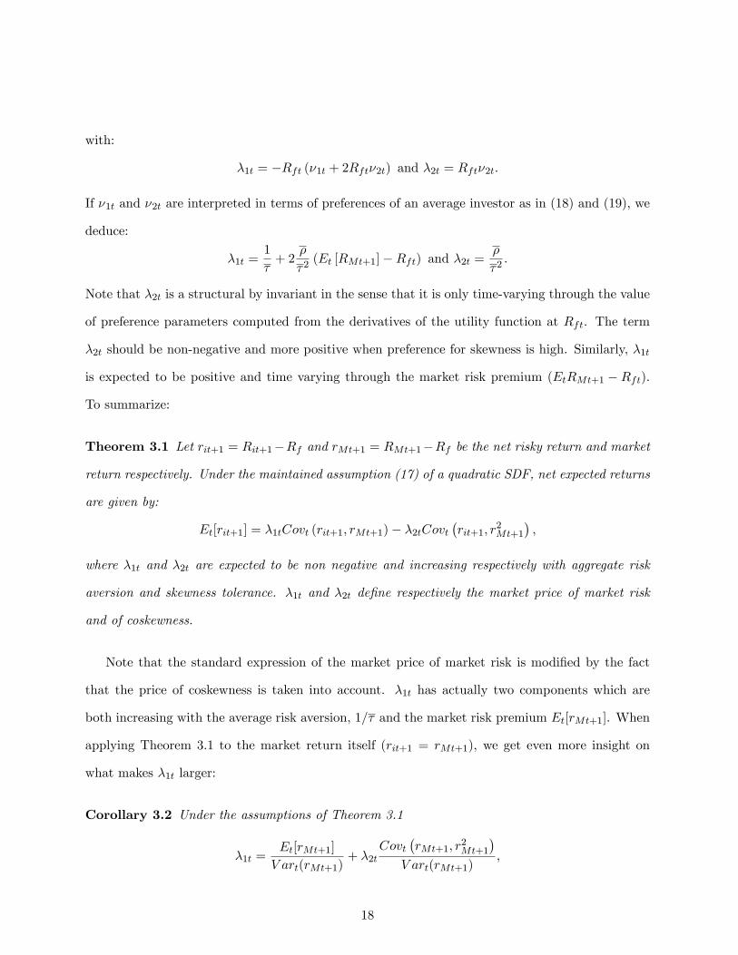
with:

�1t = �Rft (�1t + 2Rft�2t) and �2t = Rft�2t:

If �1t and �2t are interpreted in terms of preferences of an average investor as in (18) and (19), we

deduce:

�1t =1

�+ 2

�

�2(Et [RMt+1]�Rft) and �2t =

�

�2:

Note that �2t is a structural by invariant in the sense that it is only time-varying through the value

of preference parameters computed from the derivatives of the utility function at Rft. The term

�2t should be non-negative and more positive when preference for skewness is high. Similarly, �1t

is expected to be positive and time varying through the market risk premium (EtRMt+1 �Rft).

To summarize:

Theorem 3.1 Let rit+1 = Rit+1�Rf and rMt+1 = RMt+1�Rf be the net risky return and market

return respectively. Under the maintained assumption (17) of a quadratic SDF, net expected returns

are given by:

Et[rit+1] = �1tCovt (rit+1; rMt+1)� �2tCovt�rit+1; r

2Mt+1

�;

where �1t and �2t are expected to be non negative and increasing respectively with aggregate risk

aversion and skewness tolerance. �1t and �2t de�ne respectively the market price of market risk

and of coskewness.

Note that the standard expression of the market price of market risk is modi�ed by the fact

that the price of coskewness is taken into account. �1t has actually two components which are

both increasing with the average risk aversion, 1=� and the market risk premium Et[rMt+1]. When

applying Theorem 3.1 to the market return itself (rit+1 = rMt+1), we get even more insight on

what makes �1t larger:

Corollary 3.2 Under the assumptions of Theorem 3.1

�1t =Et[rMt+1]

V art(rMt+1)+ �2t

Covt�rMt+1; r

2Mt+1

�V art(rMt+1)

;

18

In particular, we can see that Theorem 3.1 coincides with the standard Sharpe-Lintner CAPM

formula when �2t = 0, that is when the average preference for skewness is zero. By contrast, �1t is

augmented in the general case by an additive term which is proportional to both �2t and market

coskewness through:

Covt�rMt+1; r

2Mt+1

�= Etr

3Mt+1 � (EtrMt+1)

�Etr

2Mt+1

�:

This notion of market coskewness has already been put forward by Harvey and Siddique (2000)

and Theorem 3.1 and Corollary 3.2 correspond to their formula (7).

It is also worth rewriting the pricing relationship of Theorem 3.1 and Corollary 3.2 in terms of

betas:

Et[rit+1] =��1tV art(rMt+1)

��iMt �

��2tV art(r

2Mt+1)

��iMt; (20)

or

Et[rit+1] = Et [rMt+1]�iMt � �2tV art(r2Mt+1) � (�iMt � �MMt�iMt) ; (21)

where

�iMt =Covt (rit+1; rMt+1)

V art(rMt+1), �iMt =

Covt�rit+1; r

2Mt+1

�V art(r2Mt+1)

:

The term �iMt is the standard market beta while the beta coe¢ cient with respect to the squared

market return is �iMt; up to a change in normalization, it corresponds to the measure of coskewness

already introduced in Section 2. Therefore, the result of equation (21) matches exactly that of

Theorem 2.8 under a conditionality.

As already shown in Section 2, the beta pricing model (20) with a second beta coe¢ cient

interpreted in terms of coskewness with the market is observationally equivalent to a conditional

version of the three-moments CAPM �rst proposed by Kraus and Litzenberger (1976) (see also

Ingersoll (1987), p. 100). In particular (21) shows, as does formula (64) in Ingersoll (1987), that

the beta pricing relationship di¤ers from Sharpe-Lintner CAPM by a factor proportional to the

di¤erence between the two betas.

For the purpose of econometric identi�cation (see Section 4), it is convenient to interpret this

di¤erence between two betas in terms of a¢ ne regressions. In the same way we de�ned in Section

19

2 the skewness portfolio from the a¢ ne regression of the squared market return on the vector of

primitive assets, it is convenient to focus here on the part of r2Mt+1 which can be mimicked by a

linear function of rMt+1, conditionally on available information at time t:

r2Mt+1 =Covt

�r2Mt+1; rMt+1

�V art (rMt+1)

rMt+1 + r(2)Mt+1:

Then r(2)Mt+1 is the part of r2Mt+1 which is orthogonal to rMt+1. It follows straightforwardly:

Theorem 3.3 We have:

Covt�rit+1; r

2Mt+1

�= V art

�r2Mt+1

�� [�iMt � �MMt�iMt] :

In other words, (21) is a signi�cant modi�cation of a common Sharpe-Lintner CAPM pricing

relationship if and only if the following two conditions are ful�lled: �rst, the market preference for

skewness is strong enough to make the skewness price �2t signi�cantly di¤erent from zero; second,

the return of asset i is signi�cantly correlated to that part of r2Mt+1 which is orthogonal to rMt+1:

Normalization in terms of the beta coe¢ cients is usually convenient, since it allows a direct

interpretation of beta loadings in terms of factor risk premium. For instance, when �2t = 0; (20)

applied to the market gives the usual formula: �1t = P(1)Mt with

P(1)Mt =

Et[rMt+1]

V art(rMt+1):

However, in general �1t and �2t cannot be read as simple risk premia associated respectively to

the two payo¤s rMt+1 and r2Mt+1. Even if we assume that r2Mt+1 does correspond to a payo¤ of a

portfolio available in the market with price �t, the risk premium on such a payo¤:

P(2)Mt (�t) =

Et

hr2Mt+1

�t

i�Rft

V art

�r2Mt+1

�t

� =Et[r

2Mt+1]�Rft�t

V art�r2Mt+1

� �t (22)

will not coincide with (��2t�t). The di¤erence comes from the fact that the two factors are not

orthogonal. The term �1t does depend on �2t (see Corollary 3.2) and the expression of �2t as a

function of the equilibrium prices is more involved:

20

Theorem 3.4 If �t = Et�mt+1r

2Mt+1

�denotes the equilibrium price of a payo¤ r2Mt+1, we have:

�2t =�MMtP

(1)Mt �

1�tP(2)Mt (�t)

1� �2t�rMt+1; r2Mt+1

� ;where according to (22), P (2)Mt (�t) is the risk premium on the asset with payo¤ r

2Mt+1 and �

2t

�rMt+1; r

2Mt+1

�denotes the square (conditional) linear correlation coe¢ cient between rMt+1 and r2Mt+1:

Note that, from (22) we have:

lim�t 0

P(2)Mt (�t)

�t=

Et[r2Mt+1]

V art�r2Mt+1

� : (23)

In this limit case, we get

�2t =�MMtP

(1)Mt �

Et[r2Mt+1]

V art(r2Mt+1)

1� �2t�rMt+1; r2Mt+1

� ; (24)

which actually coincides with the formula put forward by Harvey and Siddique (2000). However,

this limit case appears to be at odds with a no-arbitrage condition since �t = Et�mt+1r

2Mt+1

�should be strictly positive. Since, from (22),

P(2)Mt (�t)

�t=Et[r

2Mt+1]�Rft�t

V art�r2Mt+1

� ; (25)

we expect that considering the limit case (23), i.e. considering �t = 0, leads one to overestimate

P(2)Mt(�t)�t

and therefore to underestimate �2t (see Theorem 3.4).

Whether the shadow market price of r2Mt+1 is signi�cantly positive or not is an empirical ques-

tion: the relevant empirical issue (see Section 4) is then to decide if considering only the limit case

(24) leads to an economically signi�cant underestimation of the weight �2t of coskewness in the

two-factor pricing relationship (21). If it is the case, we must realize that �2t actually depends on

investors�preferences for skewness as they show up either in the (market) price of squared market

return or, equivalently as shown below, in the risk neutral variance of the market return.

3.2 Risk-Neutral Variance and the Pricing of Asymmetry Risk

In order to shed more light on the di¤erence between the general skewness-pricing formulas of

Theorem 3.4 (jointly with Theorem 3.1 and Corollary 3.2) and the limit case (24) put forward by

21

Harvey and Siddique (2000), it is worth interpreting their implied assumption ��t = 0�in terms of

market risk neutral variance.

More precisely, the conditional risk neutral variance V ar�t (RMt+1) of the market return is

de�ned from the probability density function Rftmt+1:

V ar�t (RMt+1) = Et�Rftmt+1R

2Mt+1

�� (Et (Rftmt+1RMt+1))

2

= Rft�Et�mt+1R

2Mt+1

��Rft

�= RftEtmt+1 (RMt+1 �Rft)2

= Rft�t:

In other words, quantitative assessment of �t is akin to the pricing of the �volatility contract�

R2Mt+1 (see Bakshi, Kapadia and Madan (2003)) or the direct evaluation of the market risk neutral

variance.

Typically, the risk neutral variance can be inferred from observed option prices (see Rosenberg

(2000)). For instance, in a standard conditional log-normal setting, a simple extension of Brennan

(1979) risk neutral valuation relationships (see Garcia, Ghysels and Renault (2003)) will give:

Theorem 3.5 If (logmt+1; logRMt+1) is jointly normal given the conditioning information,

V ar�t (RMt+1) = V art (RMt+1) ��

RftEtRMt+1

�2< V art (RMt+1) :

Put di¤erently, in the case of conditional log-normality, the risk neutral variance will be smaller

than the objective variance, even more so when the market risk premium is large. We want however

to argue here that in the general case, pushing the risk neutral variance to zero as in Harvey and

Siddique (2000) implicitly amounts to neglecting the possibly positive price of the component of

the volatility contract which cannot be hedged by primitive asset returns.

More precisely, we can show:

Theorem 3.6

(i) The risk neutral variance V ar�t (RMt+1) of the market return is:

V art (RMt+1) +Rft

Et�mt+1 Mt+1

��Et� Mt+1

�Rft

!+RftEt (mt+1"t+1)

22

where Mt+1 = �?skewRt+1 is the payo¤ of the skewness portfolio de�ned in Section 2 and:

"t+1 = (RMt+1 � ERMt+1)2 �

� Mt+1 � E Mt+1

�:

(ii) With a quadratic SDF

mt+1 = �0t + �1tRMt+1 + �2tR2Mt+1

we have:

Et [mt+1"t+1] = �2tV art ("t+1)

Theorem 3.6 con�rms that the di¤erence V ar�t (RMt+1)� V art (RMt+1) has two components:

The �rst component is determined by the risk premium on the skewness portfolio. As seen in

Section 2, investors with a strong skewness tolerance will want to hold this portfolio and we may

then expect a negative risk premium to be associated with it. To analyze further the sign of the risk

premium on the skewness portfolio, let us apply Theorem 2.8 to Ri = �?skewR . Straightforward

computation gives

E��?skewR

��Rf =

1

�E (RM � ERM )3 �

�

�2V ar

��?skewR

�:

In other words, only a rather unlikely strongly positive market skewness could prevent the risk

premium on the skewness portfolio from being negative. Such a negative risk premium would

explain why the risk neutral market variance may be much smaller than the objective one and even

possibly zero as in Harvey and Siddique (2000).

However, the second component of the risk neutral variance, namely Et (mt+1"t+1) ; should be

positive with a quadratic SDF . Typically, �2t = 1Rft

��2will be signi�cantly positive in the case of

high skewness tolerance, and appears to be multiplied by the part V art ("t+1) of the total variance

V art

�(RMt+1 � EtRMt+1)

2�which is not hedged by primitive assets.

This is the reason why we conclude that it is safer to consider a strictly positive risk neutral

market variance and in turn a strictly positive coe¢ cient �t in Theorem 3.4.

23

4. Empirical Illustration

4.1 The General Issue

The empirical relevance of the asset pricing model with coskewness as developed in previous sections

is encapsulated in the asset pricing equation (21):

Et [rit+1] = Et [rMt+1]�iMt � �2tV art(r2Mt+1) � (�iMt � �MMt�iMt) : (26)

The question is: does this asset pricing equation signi�cantly deviate from standard CAPM?

That is: should we maintain a signi�cantly positive skewness premium �2t?

It turns out that the statistical identi�cation of this hypothesis is di¢ cult, since, as has been

noted by Barone-Adesi, Gagliardini and Urga (2004), covariance and coskewness with the market

tend to be almost collinear across common portfolios, leading to marginally signi�cant coskewness

factors (�imt � �mmt�imt). To shed more light on this identi�cation issue, let us consider the

(conditional) a¢ ne regression of asset i�s net return on market return:

rit+1 = �it + �iMtrMt+1 + uit+1: (27)

It is clear that asset i�s coskewness can be interpreted as the covariance between the residual of

this regression with squared market return:

V art�r2Mt+1

�� (�iMt � �MMt�iMt) = Covt

�uit+1; r

2Mt+1

�= Covt

�uit+1; R

2Mt+1

�: (28)

Therefore, a positive sign for �2t can be identi�ed only insofar as one can observe some asset

returns rit+1 with positive (negative) coskewness Covt�uit+1; r

2Mt+1

�and check that they com-

mand a lower (higher) expected return than explained by standard CAPM. The problem is that

Covt�uit+1; r

2Mt+1

�will be more often than not close to zero since uit+1 is by de�nition (condi-

tionally) uncorrelated with rMt+1. Of course, non correlation does not imply independence (except

in linear market models like the Gaussian one) and one may hope that some asset i exhibits a

signi�cantly positive (or negative) covariance Covt�uit+1; r

2Mt+1

�. However, as long as a linear

approximation is valid, Covt�uit+1; r

2Mt+1

�is almost zero, which leads to:

Covt�rit+1; r

2Mt+1

�� �iMtCovt

�rMt+1; r

2Mt+1

�24

almost collinear with �iMt across portfolios.

To avoid such a perverse linearity e¤ect, Barone-Adesi, Gagliardini and Urga (2004) focus on

a quadratic market model �rst introduced by Barone-Adesi (1985). With his speci�cation they

estimate a coe¢ cient �2t, which is slightly signi�cantly positive, at least when the risk free rate is

a free parameter, not assumed to be observed by the econometrician. However, their approach is

unconditional and this may explain the di¢ culty in identifying the sign of �2t, in particular with

respect to the risk free rate issue.

To remedy that, we propose here to consider instead the asymmetric GARCH-in-mean model

recently estimated by Bekaert and Liu (2004). Since this model exhibits interesting time-varying

nonlinearities in the consumption process, it may allow an accurate identi�cation of time varying

conditional coskewness and in turn consumption-based preference for coskewness. The superior

identi�cation power of such a conditional approach will actually be con�rmed below through a

series of Monte Carlo simulations based on Bekaert and Liu�s (2004) parameter estimates.

4.2 The Simulation Set-up

Bekaert and Liu (2004) estimate a GARCH factor model with in-mean e¤ects for the trivariate

process of logarithm Xt+1 of consumption growth, logarithm of stock return Log (RMt+1) and

logarithm of bond return Log (Rft+1) :

Yt+1 = [Y1t+1; Y2t+1; Y3t+1]0 = [Xt+1; Log (RMt+1) ; Log (Rft+1)]

0 :

The model assumes the dynamics

Yt+1 = ct +AYt +et+1; (29)

where the coe¢ cient cit of ct, i = 1; 2; 3; is an a¢ ne function of V art [Yit+1] and all the time

variation in volatility is driven by time varying uncertainty in consumption growth: the conditional

probability distribution of et+1 given information It is normal with zero mean and a diagonal

covariance matrix, the coe¢ cients of which are constant except for the �rst one which follows an

25

asymmetric GARCH(1,1):

V art [e1t+1] = �1 + � (e1t)2 + �V art�1 [e1t] + � (Max [0;�e1t])2 : (30)

To limit parameter proliferation, they assume that all the o¤-diagonal coe¢ cients of the matrix

are zero except in the �rst column; in other words the consumption shock is the only factor. For

the sake of normalization, the diagonal coe¢ cients of are �xed to the value 1. Table 2 gives the

estimated parameters provided by Bekaert and Liu (2004) on monthly US data. These estimates

will be considered below as true population values for simulating a sample path.

A convenient feature of the above model for our purpose is that, since it maintains a condi-

tional joint normality assumption for log-consumption and log-market return, it allows us to apply

Theorem 3.7 to assess the risk neutral variance without need of a preference speci�cation. More

precisely, insofar as the log-pricing kernel is, given information It; a linear combination of the �rst

two components of Yt+1, as it is not only in the Lucas (1978) consumption based CAPM with

isoelastic preferences but also more generally in the Epstein and Zin (1991) recursive utility model,

we are sure that Theorem 3.7 applies.

Then, our simulation set-up is as follows: for a given simulated path of the process (Yt+1), spec-

i�cations (29) and (30) allow us to compute iteratively corresponding paths �rst of V ar�t (RMt+1) =

V art (RMt+1) [Rft=Et (RMt+1)]2, then of �t = V ar�t (RMt+1) =Rft, of

P(2)Mt(�t)�t

=Et[r2Mt+1]�V ar�t (RMt+1)

V art(r2Mt+1),

of P (2)Mt (�t), and �nally of �2t according to Theorem 3.4. We recall that the limit case put forward

by Harvey and Siddique (2000) corresponds to the alternative formula:

�HS2t = MMtP

(1)Mt �

Etr2Mt+1

V art(r2Mt+1)

1� �2t�rMt+1; r2Mt+1

� :

The path of this value is also easily built from the above simulation.

Of course, by introducing only one risky asset, this setting does not allow us to compare coskew-

ness across portfolios. However, we vary exogenously both the asset i�s beta and coskewness and

compare the relative expected return error of Harvey and Siddique (2000) and the CAPM model

with respect to the expected return decomposition given in our model (see equation 20).

26

The focus of our interest here is to get time-series of �2t and �HS2t , in order to assess their sign

and their di¤erences both date by date and in average. Note moreover, that return skewness in

this market is not as trivial as log-normality may lead one to think. Over two periods, temporally

aggregated asset returns will feature some sophisticated skewness, �rst due to the asymmetric e¤ect

in the variance dynamics and second due to time varying risk premium. A detailed characterization

of induced dynamic skewness pricing is beyond the scope of this paper.

4.3 Monte Carlo Results

When drawing time series from the Bekaert and Liu (2004) estimated model described above,

several experiments are performed.

First, a long time series for say a 500 month-long path, is informative in several respects. Due

to the stationarity of the stochastic processes of interest, time-averages over 500 months allow us to

compare conditional and unconditional quantities. Moreover, the dynamic features of the observed

simulated path are of interest.

Of course, one could argue that our conclusions are only valid for one particular simulated

path. This is the reason why we also perform an extensive Monte Carlo experiment by simulating

1000 sample paths, each one with a length of 500 months. This will allow us to show that cross-

simulation variability is su¢ ciently small to ensure the robutness of conclusions drawn from one

speci�c simulated path.

Note that, since conditional pricing is our focus of interest, it would be meaningless to want to

assess it through averages over a large number of paths. For instance, volatility clustering must

be assessed on a given sample path while averaging across paths would push volatility towards its

constant unconditional mean. For the same reason, we are going to see that the market price of

coskewness is signi�cant only with a conditional point of view. This is the reason why we study in

particular a single 500 month-long simulated path throughout this section.

Figure 1 displays the associated sample paths for both the market price of coskewness �2t (as

characterized by Theorem 3.4) and of its limit value �HS2t de�ned by (24). See Table 2 for same

summary statistics.

27

A �rst striking observation is that while the �2t path con�rms that the market price of coskew-

ness is positive (4:25 on average), the �HS2t path diaplays some implausibly hugely negative prices

of coskewness (�67:82 on average). In other words, neglecting the price �t of squared net returns

leads to a severe underestimation of the price of coskewness, so severe that it may reverse the

direction of the e¤ect of coskewness in asset prices.

This conclusion is statistically signi�cant and not related to a speci�c sample path. According

to Table 3, the cross-paths standard deviation of the time-average of �2t over 1000 simulated paths

is only 0:2758 (for a general average of 4:2917) while it is only 0:5388 for �HS2t (for a general average

of �67:7317).

As explained in Section 3.1, the reason why �HS2t is too small is that it overestimates the risk

premium P(2)Mt(�t)�t

on the squared market return. It is worth noticing that the correct formula (22)

always leads to a nonnegative risk premium on the squared net market return as displayed on

Figure 2. However, by contrast with the limit case considered by Harvey and Siddique (2000), the

shadow price �t of the squared net market return is signi�cantly positive: 0:64% on average with

a standard deviation (of time-averages over 1000 simulated paths) of only 0:00052%.

As already pointed out, the advantage of considering a speci�c simulated path is to enhance

the di¤erences between conditional and unconditional quantities. While the time series of �2t does

show a positive average price of 4:25 for coskewness (4:2917 among 1000 paths), it comes with a

standard deviation error of 0:2758 (average value of standard deviations over 1000 paths is equal

to 4:06).

This result may explain why Barone-Adesi, Gagliardini and Urga (2004) had such di¢ culty in

identifying a positive price in an unconditional setting. They actually get a t-statistic of 1:01, which

has the same order of magnitude as our informal assessment. Of course, a rigorous unconditional

study should not be simply based on time-averages. By contrast, Figure 1 shows that spot values

of the process series �2t may cover the full interval between 0 and 20, making them likely signi�cant

for a number of dates. This enhances the important contribution of Harvey and Siddique (2000)

who stress that coskewness pricing must be addressed in a conditional setting. However, even

28

an unconditional approach would not make the simpli�ed price series �HS2t meaningful, since their

standard error is only 7:45, which does not compensate for their negative average of �67:82.

Overall, we conclude that there should be a positive price for coskewness, but that it is not high

and di¢ cult to identify in an unconditional setting. One way to interpret the limited level of this

price is to realize that buying the squared net market return commands a positive risk premium

(see Figure 2) which, by Theorem 3.4 results in a decrease in the price �2t. This does not mean

that skewness is worthless, but only that, by (26), a part of its value is already captured by the

linear pricing of squared return. In other words, a positive skewness implies a positive correlation

between market return and squared market return, so that the two components of asset prices

cannot be interpreted separately.

Of course, one ought to realize that quadratic pricing kernels cannot be more than local approx-

imations of a true pricing kernel, for instance, as in the neighborhood of small risk as in Section

2. In particular, while a representative agent with a convex utility function would imply that the

pricing kernel is decreasing with respect to the market return, this cannot be the case on the full

range of returns with a quadratic function. More precisely, a quadratic pricing kernel as character-

ized by (17), (18), and (19) with a positive coskewness price �2t will become increasing when the

market returns exceed its conditional expectation by more than (�=2�). This kind of paradoxical

increasing shape of pricing kernels for large levels of market return already surfaced in the empirical

evidence documented by Dittmar (2002). Of course, a negative �2t, as in the case of the zero-price

�t approximation, would produce an even more bizarre behaviour, with an increasing pricing kernel

for any value of the market return below its expectation.

As far as Dittmar�s paradox is concerned, it does not mean that one should give up nonlinear

polynomial pricing kernels because their decreasing shape cannot be enforced on the whole range of

possible market returns. One must only remember that polynomial approximations are local and

ought to be used cautiously. For instance, it is clear that market information about risk neutral

variance or equivalently about the price �t of squared net market return may be helpful for a better

control of a quadratic pricing kernel on the range of interest. Since this information may be in

29

practice backed out from derivative asset prices, it is worth checking how it works on simulated

paths. Figure 3 displays the pricing kernel surface as well as its time average as a function of the

net market return. This �gure is obtained with our value of �t (time average of 0:64%) which

determines the coe¢ cients �1t and �2t of the pricing kernel by application of Corollary 3.2 and

Theorem 3.4. No paradoxical behaviour of the pricing kernel is observed in this �gure: on the

range of interest for the net market return, the pricing kernel is always decreasing. If one now

increases the value of �t, by �xing somewhat arbitrarily the price of the squared market return at

the level 1:02, which in turn implies a time-varying �t (with a time average of 1:56%), one gets the

results shown in Figure 4. Then, one may observe that, by contrast with Figure 3, on the same

range of values of the market return, the aforementioned increasing shape of the pricing kernel for

large returns may show up. While Figures 3 and 4 are about time averages over one particular

sample path, the general average and the standard deviation of these time averages are computed

over 1000 sample paths. This leads to the pricing kernel plots with 5% con�dence bounds provided

in �gures 5 and 6.

Finally, to assess the economic signi�cance of the pricing improvements brought by our model,

we compare it with both the limit case of Harvey and Siddique (2000) (HS hereafter) and with a

standard CAPM as well. In order to do this, we plot as functions of characteristics a hypothetical

asset i (coe¢ cient beta-i and coskewness delta-i ), the relative errors on expected returns between

our model and CAPM (Figure 7) and between our model and HS (Figure 8). Not surprisingly,

the CAPM risk premium may be too high in the case of a joint occurrence of positive betas

and positive coskewness. Typically, our model predicts that a positive coskewness, since it meets

investors�concern for positive skewness, may slightly erase the role of market beta as a measure of

risk to be compensated. Note however that the relative pricing errors of CAPM do not exceed 1

or 2 per-cent. Pricing errors of the HS speci�cation may be much more signi�cant. They may be

between 10 and 20 per-cent when a large positive coskewness is not well taken into account due to

the negative sign �HS2t .

30

5. Conclusion

This paper investigates the relevance of non-linear pricing kernels both at the theoretical and

empirical level. We �rst show that considering pricing kernels that are quadratic functions of the

market return is a well-founded approximation of actual expected utility behaviour, at least to

characterize locally the demand for risky assets in the neighborhood of zero risk. Such quadratic

pricing kernels disclose some pricing for skewness, but only through coskewness with the market.

Heterogeneous agents hold the market portfolio and the skewness portfolio, the latter being the

�closest�portfolio to the squared market return. The skewness portfolio is based on all third-order

cross moments; in other words, while taking heterogeneity of skewness preferences into account

yields separation theorems where an additional fund emerges in asset demands, it remains true

that idiosyncratic risk is not priced, both in terms of variance and skewness.

While statistical identi�cation of a positive skewness premium may be di¢ cult since covariance

and coskewness tend to be almost collinear across common portfolios, we showed through simulated

data based on an actual estimation of a factor GARCH-in-mean model that a conditional set-up

is much more informative to capture relevant nonlinearities in pricing kernels. Such nonlinearities

imply some level of risk-neutral variance for the market which cannot be neglected. This observation

leads us to a generalization of the Harvey and Siddique (2000) beta pricing model for skewness; in

contrast with theirs, our model considers the price of the squared market return as a free parameter

whose actual value might be backed out of observed derivative asset prices.

Although conditional, our study is purely statistical in the sense that investors only maximize

a one-period utility function. Typically, while only conditional skewness of asset returns show up

in the current paper, a multiperiod setting would also enhance the role of dynamic asymmetry,

that is some instantaneous correlation between asset returns and their volatility process. Such an

e¤ect has been dubbed the leverage e¤ect by Black (1976) and speci�c leverage-based dynamic risk

premia should be the result of non-myopic intertemporal optimization behaviour of investors with

preferences for skewness.

31

6. Appendix

Proof of theorems 2.2 and 2.4. The solution ! (�) = (!i (�))1�i�n of problem (2) determines

a terminal wealth

W (�) = Rf +nXi=1

!i (�) (Ri �Rf )

according to the �rst order conditions

0 = E�u0 (W (�)) � (Ri �Rf )

�= E [hi (�)] : (31)

Then, setting

hi (�) = u0 (W (�)) � (�ai (�) + Yi) ;

this implies that Ehdhid� (�)

i= 0 and so that lim� 0+ E

hdhid� (�)

i= 0. Writing out the last equality

we getnXi=1

!i (0)Cov (Yi; Yk) = �u0 (Rf )

u00 (Rf )ak (0) :

Using the variance-covariance matrix � of the vector Y of random variables and the de�nition of

the risk neutral tolerance in (6) we get ! (0) = ��1 � � � a (0), which ends the proof of Theorem 2.2.

To prove Theorem 2.4 we take the second-order derivatives of equation (31) and get

lim� 0+

E

�d2hid2�

(�)

�= 0:

Writing this out and using de�nition (6) we get:

nXi=1

!0i (0)Cov (Yi; Yk) =�

�

nXi=1

!2i (0)E[Y2i Yk] + 2

�

�

nXi<j

!i (0)!j (0)E[YiYjYk] + �a0k (0) (32)

=�

�

1

�2Cov

��!? (0)R

�2; Yk

�+ �a0k (0) :

Therefore equation (32) reads

!0 (0) = ���1�c (! (0))

�

�21

�2V ar

h!?R

i+ a0 (0)

�= ���1

�c (! (0))

�

�21

�2

h�a? (0)��1

��2�

���1�a (0)

i+ a0 (0)

�= ���1

�c (! (0)) �P 2 (0) + a0 (0)

�:

32

Proof of theorems 2.5 and 2.6. Using the de�nitions of � s, �s from equation (9), the demand

equation (10) and the �rst market-clearing equation in (13) we derive from the condition

S! =SXs=1

!s (0) =SXs=1

��1� sa (0)

that

a (0) =1

��!: (33)

Using the results of Theorem 2.2 that !s (0) = ��1� sa (0), this implies

!s (0) =� s�!:

Looking at equation (8) we then check that ck (!s (0)) = ck (!). Using (32) and the second market-

clearing equation in (13) we get from

SXs=1

!0s (0) =SXs=1

� s��1 �c (!) �sP 2 (0) + a0 (0)� = 0

that

a0 (0) = ��c (!)P 2 (0) :

Thus:

a0k (0) = ��ck (!)P 2 (0) : (34)

Plugging (34) into Theorem 2.4 gives:

!0s (0) = � s��1 �c (!) �sP 2 (0) + a0 (0)� = � s [�s � �]P 2 (0)��1c (!) :

We �nd:

P 2 (0)��1c (!) c (!) =1

�P 2 (0)��1

Cov�R;�!? (R� ER)

�2�V ar

�!? (R� ER)

�=

1

��2P 2 (0) (V ar (R))�1

Cov�R;�!? (R� ER)

�2�V ar

�!? (R� ER)

�=

1

�(V ar (R))�1Cov

�R;�!? (R� ER)

�2�Given that RM = !?R,

P 2 (0)��1c (!) c (!) =1

�(V ar (R))�1Cov

�R; (RM � ERM )2

�33

Therefore

�!0s (0) = � s [�s � �] (V ar (R))�1Cov�R; (RM � ERM )2

�is ends the proof.

Proof of theorem 2.7. We �rst �nd two real numbers L and N such that, with

m (�) =1

Rf+ L �

�RM (�)� E[RM (�)]

�+N �

�(RM (�)� E[RM (�)])2 � E (RM (�)� E[RM (�)])2

�;

we have:

Em (�) ���2a (�) + �Y

�= 0:

That is we require:1

Rf�2a (�) + �Cov (Y;m (�)) = 0:

We want to see these equations ful�lled with a (�) = a (0) + �a0 (0) where a (0) and a0 (0) given by

Theorem 2.5. Then:

1

Rf

�2

��! � 1

Rf�3�P 2 (0) c (!)

+ L � Cov (R;RM (�)) +N � Cov�R; (RM (�)� E[RM (�)])2

�= 0:

Let us de�ne L and N such that

L � Cov (R;RM (�)) = � 1

Rf

�2

��!;

N � Cov�R; (RM (�)� E[RM (�)])2

�=

1

Rf�3�P 2 (0) c (!) :

Noticing that

�2�! = Cov (R;RM (�)) ; and

��3P 2 (0) c (!) = �V ar (RM )

�c (!) =

1

�Cov

�R; (RM (�)� E[RM (�)])2

�;

we conclude that

L = � 1

Rf�; and N =

1

Rf

�

�2

34

Second, since the pricing kernel correctly prices the primitive assets:

Em (�)R = 1

it can be replaced by its projection on the set of primitive assets and the market return:

m (�) = E (m (�) jRM ; R)

=1

Rf� 1

Rf�(RM (�)� ERM (�)) +

�

Rf�2�

?skew (R� E (R))

where

�skew = (V ar (R))�1Cov

�R; (RM � ERM )2

�which is the announced result.

Proof of theorem 2.8. Note that

E[Ri]�Rf = �ai (�) = �ai (0) + �3a0i (0) :

Then, by theorem 2.5, the vector (ERi �Rf )1�i�n can be written as:

�

��! � �3�P 2 (0) c (!) = 1

�Cov (R;RM )�

�

�2Cov

�R; (RM � E[RM ])2

�:

From theorem 2.6, we have

�skew = (V ar (R))�1Cov

�R; (RM � ERM )2

�Thus

Cov�R;�?skewR

�= Cov

�R; (RM � ERM )2

�Hence,

�

��! � �3�P 2 (0) c (!) = 1

�Cov (R;RM )�

�

�2Cov

�R;�?skewR

�De�ning

i =Cov

�Ri;�

?skewR

�V ar

��?skewR

�we deduce for each i = 1; :::;K:

E[Ri]�Rf =1

�Cov (R;RM )�

�

�2V ar

��?skewR

� i

which corresponds to the formula of Theorem 2.8.

35

Proof of Theorem 3.4. By applying (26) to the net return on the squared market return payo¤

rit+1 =r2Mt+1

�t�Rft

we get

Et[r2Mt+1]�Rft�t = Et[rMt+1]�MMt

V ar�r2Mt+1

�V ar (rMt+1)

� �2t � V ar�r2Mt+1

���1� �2t

�rMt+1; r

2Mt+1

��;

that is:P(2)Mt

�t= �MMtP

(1)Mt � �2t

�1� �2t

�rMt+1; r

2Mt+1

��:

This gives the announced value for �2t.

Proof of Theorem 3.5. Assume that the joint process�mt+1; R

;t+1

�is conditionally lognormal.

Then, "Log (mt+1)

LogRMt+1

#=It N

""�mt

�Mt

#;

"�2t �mrt

�mrt �2Mt

##:

Let us denote

cmt = Etmt+1R2Mt+1:

The market return risk neutral variance V ar�t (RMt+1) is

V ar�t (RMt+1) = E�tR2Mt+1 �R2ft; with E�tR

2Mt+1 = RftEtmt+1R

2Mt+1:

We know that

Log�mt+1R

2Mt+1

�= Log (mt+1) + 2Log (RMt+1) :

Therefore,

Et[mt+1R2Mt+1] = exp

��mt + 2�Mt + 0:5�

2t + 2�

2Mt + 2�mrt

�= exp

���mt � 0:5�2t

�exp

�2�Mt + 2�

2Mt

�exp

��2�Mt � �2Mt

��

��exp

��mt + �Mt + 0:5�

2t + 0:5�

2Mt + �mrt

��2:

But Et[mt+1 �RMt+1] = 1 is equivalent to

exp��mt + �Mt + 0:5�

2t + 0:5�

2Mt + �mrt

�= 1;

36

and therefore

Et[mt+1R2Mt+1] = exp

���mt � 0:5�2t

�exp

�2�Mt + 2�

2Mt

�exp

��2�Mt � �2Mt

�= Rft

ER2Mt+1

(EtRMt+1)2 :

Consequently,

V ar�t (RMt+1) = R2ftEtR

2Mt+1

(EtRMt+1)2 �R

2ft = V art (RMt+1)

�Rft

EtRMt+1

�2< V art (RMt+1) :

Proof of Theorem 3.6. Assume that

mt+1 = �0t + �1tRMt+1 + �2tR2Mt+1:

We denote

"t+1 = (RMt+1 � ERMt+1)2 � E

h(RMt+1 � ERMt+1)

2 jRt+1i

the residual of the linear regression of (RMt+1 � ERMt+1)2 on RMt+1. This residual can be written

as:

"t+1 = (RMt+1 � ERMt+1)2 �

� Mt+1 � E Mt+1

�with

Mt+1 = Eh(RMt+1 � ERMt+1)

2 jRt+1i

Note that:

Mt+1 = �?skewRt+1

Therefore,

Covt (mt+1; "t+1) = �2tV art ("t+1) :

37

References

[1] Bakshi, G., N. Kapadia, and D. Madan. 2003. �Stock Return Characteristics, Skew Laws, and

Di¤erential Pricing of Individual Equity Options.�Review of Financial Studies 16: 101-143.

[2] Bakshi, G., and D. Madan. 2000. �Spanning and Derivative Security Valuation.� Journal of

Financial Economics 55: 205-238.

[3] Barone-Adesi, G. 1985. �Arbitrage Equilibrium with Skewed Asset Returns.� Journal of Fi-

nancial and Quantitative Analysis 20: 299-313.

[4] Barone-Adesi, G., G. Urga, and P. Gagliardini. 2004. �Testing Asset Pricing Models with

Coskewness.�Journal of Business and Economic Statistics 22: 474-485.

[5] Bekaert, G., and J. Liu. 2004. �Conditioning Information and Variance Bounds on Pricing

Kernels.�The Review of Financial Studies 17: 339-378.

[6] Black, F. 1976. �The Pricing of Commodity Contracts.� Journal of Financial Economics 3:

167-179.

[7] Brennan, M. J. 1979. �The Pricing of Contingent Claims in Discrete Time Models.�Journal

of Finance 24: 53-68.

[8] Chabi-Yo, F., E. Ghysels, and E. Renault. 2007. �Disentangling the E¤ects of Heterogeneous

Beliefs and Preferences on Asset Prices.�Discussion paper, UNC.

[9] Cochrane, J.H. 2001. Asset Pricing. Princeton University Press.

[10] Dittmar, R. F. 2002. �Nonlinear Pricing Kernels, Kurtosis Preference, and Evidence from

Cross section of Equity Returns.�Journal of Finance 57: 368-403.

[11] Epstein, L., and S. Zin. 1991. �Substitution, Risk Aversion and the Temporal Behaviour of

Consumption and Asset Returns: An Empirical Analysis.�Journal of Political Economy 99:

263-286.

38

[12] Garcia, R., E. Ghysels, and E. Renault. 2003. The Econometrics of Option Pricing, in Y. Ait

Sahalia and L. P. Hansen, ed.: The Handbook of Financial Econometrics (North Holland,

forthcoming)

[13] Hansen, L., and S. Richard. 1987. �The Role of Conditioning Information in Deducing Testable

Restrictions Implied by Dynamic Asset Pricing Models.�Econometrica 55: 587-613.

[14] Harvey, C.R., and A. Siddique. 2000. �Conditional Skewness in Asset Pricing Tests.�Journal

of Finance 55: 1263-1295.

[15] Ingersoll, J. 1987. Theory of Financial Decision Making. New Jersey: Rowman & Little�eld.

[16] Jobson, J. D., and B. M. Korkie. 1982. �Potential Performance and Tests of Portfolio E¢ -

ciency.�Journal of Financial Economics 10: 433-466.

[17] Juud, G., and S. Guu. 2001. �Asymptotic Methods for Asset Market Equilibrium Analysis.�

Economic Theory 18: 127-157.

[18] Kimball, M. 1990. �Precautionary Saving in the Small and in the Large.�Econometrica 58:

53-73.

[19] Kraus, A., and R. H. Litzenberger. 1976. �Skewness Preference and the Valuation of Risk

Assets.�Journal of Finance 31: 1085-1100.

[20] Lucas, R. Jr. 1978. �Asset Prices in an Exchange Economy.�Econometrica 46: 1429-1445.

[21] Markowitz, H. 1952. �Portfolio Selection.�Journal of Finance 7: 77-91.

[22] Rosenberg J. 2000. �Asset Pricing Puzzles: Evidence from options markets.�Stern School of

Business Working Paper.

[23] Samuelson, P. A. 1970. �The Fundamental Approximation Theorem of Portfolio Analysis in

Terms of Mean, Variance and Higher Moments.�Review of Economic Studies 37: 537-42.

39

Notes

1Dittmar (2002) and Barone-Adesi, Urga, and Gagliardini (2004) study if skewness risk is priced and its price.

Chang, Johnson, and Schill (2004) test whether Fama-French factors proxy for skewness and higher moments.

2He studied a series of economies di¤ering only by the amount of risk; the case of in�nitesimal risk is the limit

economy where all risk vanishes.

3A work that also extends Samuelson�s analysis is Judd and Guu (2001). They present an asymptotically valid

theory for the trade-o¤ between one risky asset and the riskless asset in single period setups. However, while their

approach is based on bifurcation theory, our results are based directly on limits of �rst-order conditions. Futhermore

their interest is on two-agent economies with a single risky asset and potentially a derivative written on it; they do

not study stochastic discount factors.

4Samuelson (1970) provides a heuristic explanation of (1) that is of interest for readers accustomed to continuous-

time �nance models; he couches this in terms of Brownian motion and identi�es � with the square root of time.

40

0 50 100 150 200 250 300 350 400 450 500−100

−80

−60

−40

−20

0

20

40

t

λ 2t

CLRHS

Figure 1: Price of coskewness inferred from a simulated time-series of the Factor GARCH-in-mean

used in Bekaert and Liu (2004). HS indicates the price of coskewness corresponding to Harvey and

Siddique (2000); CLR indicates the price of coskewness corresponding to our formula.

41

0 50 100 150 200 250 300 350 400 450 500−0.01

0

0.01

0.02

0.03

0.04

0.05

0.06

0.07

0.08

0.09

t

PM

t(2

)

Figure 2: Risk premium on the squared net return inferred from a simulated time-series of the

Factor GARCH-in-mean used in Bekaert and Liu (2004)

42

−0.1 −0.05 0 0.05 0.1 0.150.5

0.6

0.7

0.8

0.9

1

1.1

1.2

1.3

1.4

1.5

x

m(x

)

Figure 3: Quadratic pricing kernel inferred from a simulated time-series of the Factor GARCH-in-

mean used in Bekaert and Liu (2004). In the upper graph, we plot the pricing kernel mt+1 as a

function of time and rMt+1. In the lower graph we plot the average pricing kernel �Tt=11Tmt+1.

43

−0.1 −0.05 0 0.05 0.1 0.150

0.5

1

1.5

2

2.5

3

3.5

4

x

m(x

)

Figure 4: Fixing the price of the squared market return at the level 1.02, which in turns implies

a time varying �t, we infer the quadratic pricing kernel from a simulated time-series of the Factor

GARCH-in-mean used in Bekaert and Liu (2004). In the upper graph, we plot the pricing kernel

mt+1 as a function of time and rMt+1 = x. In the lower graph, we plot the average pricing kernel

�Tt=11Tmt+1.

44

−0.1 −0.05 0 0.05 0.1 0.150.5

0.6

0.7

0.8

0.9

1

1.1

1.2

1.3

1.4

1.5

x

m(x

)

Figure 5: We plot the average of pricing kernels inferred from a simulated time-series of the Fac-

tor GARCH-in mean model: m (x) = 1K

KXk=1

1T

TXt=1

m(k)t (x)

!where T represents the number of

simulated time series of return and K = 1000 the number of replications. For each replication, we

simulated a time-series of T = 500 observations. 1T

TXt=1

m(k)t (x) is the average pricing kernel for the

kth replication. The number of replication is K = 1000. We also plot the average pricing kernel

5% con�dence interval.

45

−0.1 −0.05 0 0.05 0.1 0.150

0.5

1

1.5

2

2.5

3

3.5

4

x

m(x

)

Figure 6: We plot the average of pricing kernels inferred from a simulated time-series of the Factor

GARCH-in mean model when the price of the squared market return is �xed at the level of 1.02

which in turns implies a time-varying �t: m (x) =1K

KXk=1

1T

TXt=1

m(k)t (x)

!where T represents the

number of simulated time series of return and K = 1000 the number of replications. For each

replication, we simulated a time-series of T = 500 observations. The number of replication is

K = 1000. 1T

TXt=1

m(k)t (x) is the average pricing kernel for the kth replication. We also plot the

average pricing kernel 5% con�dence interval.

46

−5−4

−3−2

−10

12

34

5

−5

0

5−0.015

−0.01

−0.005

0

0.005

0.01

0.015

0.02

δi

Pricing Error CAPM/CLR

βi

Figure 7: For each replication, we compute the relative expected return error of the CAPM versus

the expected return given by the CLR model (see equation (20)) as a function of �iMt and �iMt:

((EtRit+1)CAPM � (EtRit+1)CLR) = (EtRit+1)CLR .

We then compute the average of the relative expected return error over K replications and plot the

average of the relative expected return error as a function of the asset i0s beta and coskewness.

47

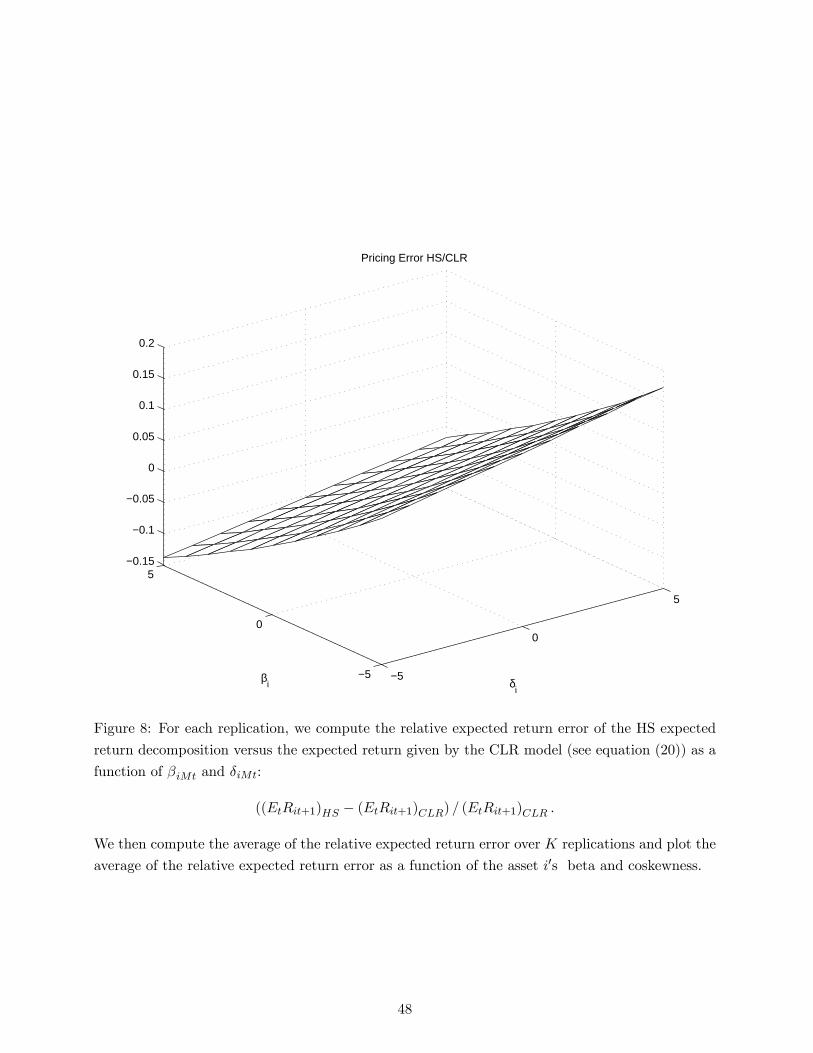
−5

0

5

−5

0

5−0.15

−0.1

−0.05

0

0.05

0.1

0.15

0.2

δi

Pricing Error HS/CLR

βi

Figure 8: For each replication, we compute the relative expected return error of the HS expected

return decomposition versus the expected return given by the CLR model (see equation (20)) as a

function of �iMt and �iMt:

((EtRit+1)HS � (EtRit+1)CLR) = (EtRit+1)CLR :

We then compute the average of the relative expected return error over K replications and plot the

average of the relative expected return error as a function of the asset i0s beta and coskewness.

48

Equations Coe¢ cients

ct Y1t Y2t Y3t

Y1t+1 0:0030 0:361 �0:029 0:008

(0:0005) (0:033) (0:022) (0:005)

Y2t+1 0:0056-162:65V art [e1t+1] �0:198 0:738 �0:0002(0:0006) (0:0001) 0:031 (0:037) (0:0043)

Y3t+1 0:0188� 58:02V art [e1t+1] �1:734 1:029 0:077

(0:0083) (0:0003) 0:005 (0:014) (0:034)

constant � � �

V art (e1t+1) 0:000019 �0:0265 0:0008 0:2705

0:000018 (0:0807) (0:7898) (0:0426)

�2 0:000014 0 0 0

(0:000002)

�3 0:006134 0 0 0

(0:00103)

�13 = �0:0564 �12 = 3:182

(0:1425) (0:003)

Table 1: This table reproduces the results of the Factor GARCH in mean estimated by Bekaert

and Liu (2004). Here �2 = V art (e2t+1) and �3 = V art (e3t+1).

K = 1 replication

Parameters Mean standard deviation

�t 0:64% 0:0076413%

�2t 4:25 4:06

�2t � �2t�1 �67:82 7:45

�HS2t 0 4:93

�HS2t � �HS2t�1 0 8:75

Table 2: Summary statistics for one particular Monte-Carlo simulation

49

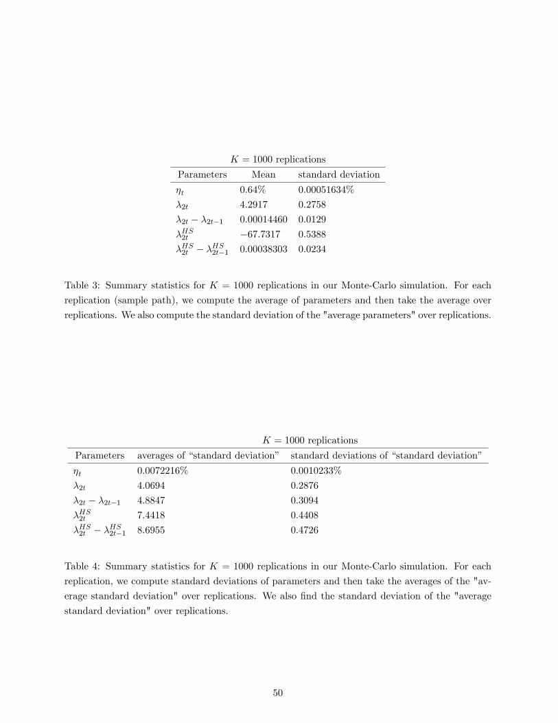
K = 1000 replications

Parameters Mean standard deviation

�t 0:64% 0:00051634%

�2t 4:2917 0:2758

�2t � �2t�1 0:00014460 0:0129

�HS2t �67:7317 0:5388

�HS2t � �HS2t�1 0:00038303 0:0234

Table 3: Summary statistics for K = 1000 replications in our Monte-Carlo simulation. For each

replication (sample path), we compute the average of parameters and then take the average over

replications. We also compute the standard deviation of the "average parameters" over replications.

K = 1000 replications

Parameters averages of �standard deviation� standard deviations of �standard deviation�

�t 0:0072216% 0:0010233%

�2t 4:0694 0:2876

�2t � �2t�1 4:8847 0:3094

�HS2t 7:4418 0:4408

�HS2t � �HS2t�1 8:6955 0:4726

Table 4: Summary statistics for K = 1000 replications in our Monte-Carlo simulation. For each

replication, we compute standard deviations of parameters and then take the averages of the "av-

erage standard deviation" over replications. We also �nd the standard deviation of the "average

standard deviation" over replications.

50