implementing sap business planning and … sap business planning and consolidation 900 pages, ......

Reading SampleNew to this edition, Chapter 10 discusses the end-to-end process to set up a basic embedded SAP BPC planning scenario. Learn how to set it up and use MultiProviders, composite providers, DataStore objects, and local providers.

Peter Jones, Tim Soper

Implementing SAP Business Planning and Consolidation900 Pages, 2015, $79.95/€79.95 ISBN 978-1-4932-1179-1

www.sap-press.com/3711

“Embedded SAP BPC Architecture”

Contents

Index

The Authors

First-hand knowledge.

© 2015 by Galileo Press, Inc. This reading sample may be distributed free of charge. In no way must the file be altered, or individual pages be removed. The use for any commercial purpose other than promoting the book is strictly prohibited.

https://www.sap-press.com/implementing-sap-business-planning-and-consolidation_3711/?utm_source=AWS&utm_medium=readingsample&utm_campaign=Browse%20the%20Book&utm_content=1179

639

Before we move too far into our coverage of embedded SAP BPC, we should examine its architecture—the SAP BW tables, queries, and Inte-grated Planning objects that will be used moving forward.

10 Embedded SAP BPC Architecture

Embedded SAP BPC provides quite a bit of flexibility and options to meet cus-tomer planning and reporting requirements. Sometimes, we have so manyoptions that half the challenge is figuring out when to use each one! As we gothrough this chapter, we’ll emphasize a given business scenario first, discuss itsarchitecture second, and then go through the configuration steps third.

In this chapter, we’ll discuss the end-to-end process to set up a basic embeddedSAP BPC planning scenario. We’ll go through the buildup of the SAP BusinessWarehouse (SAP BW) InfoProviders, the Integrated Planning (IP) objects, the SAPBW Planning Query, and then how to use the query and a basic planning functionin the SAP Enterprise Performance Management (EPM) add-in. After that, we’lltalk about how MultiProviders, DataStore objects (DSOs), and local providers canbe used in planning scenarios as well.

10.1 Setting Up the Embedded Planning Model

In this section, we’ll go through the use cases and set up of a real-time InfoCube,the IP objects, the SAP BPC objects, and the EPM add-in report and action panefrom start to finish. The main idea in this first pass is to give you a feel for howthe components work together in an end-to-end scenario and do the deep divelater in Chapter 11 and Chapter 13 on reporting and planning and forecasting,respectively.

You need the following components for a planning scenario:

� Real-time InfoCube

� Aggregation level

Embedded SAP BPC Architecture

640

10

� Planning function

� Planning-enabled query

� Embedded environment

� Embedded model

� EPM workbook with an EPM report and a planning function

10.1.1 Using Real-Time InfoCubes

InfoCubes represent a type of activity, whether it’s being used for reporting orplanning. It has a group of homogeneous characteristics and key figures to meetthe task at hand. Recall that real-time InfoCubes are write-optimized InfoCubes;they are the primary tables used in embedded SAP BPC 10.1.

As a point of reference, in standard SAP BPC, the real-time InfoCube is generatedwhen you create the model; it can only use InfoObjects in the SAP BPCnamespace, and only one key figure is allowed. So if we compare real-time Info-Cubes used for the embedded version to real-time InfoCubes used for the stan-dard version, four main differences stand out:

� Embedded InfoCubes use standard InfoObjects.

� Embedded InfoCubes can have multiple key figures.

� Embedded InfoCubes are created from SAP BW, not SAP BPC.

� Embedded InfoCubes use the normal SAP BW namespace.

As a result, using normal SAP BW objects means that you can share data more eas-ily, resulting in less data redundancy, and you can use more than one key figure,which provides data modeling flexibility.

But using real-time InfoCubes in embedded SAP BPC involves a bit more discus-sion than it did in standard SAP BPC. With standard, when you create a model,the system generated the real-time InfoCube and associated MultiProvider auto-matically. Recall from Chapter 3 that each standard model always has one corre-sponding real-time InfoCube and one MultiProvider. In embedded, you createthe real-time InfoCube first, and then you create the SAP BPC model. Further-more, embedded SAP BPC models can use one or more real-time InfoCubes,DSOs, local providers, and VirtualProviders, so now it’s much easier to mergedata from multiple sources.

Setting Up the Embedded Planning Model

641

10.1

Despite the fact that standard SAP BPC models can use different types of InfoPro-viders, real-time InfoCubes will remain the primary choice because DSOs, localproviders, and virtual InfoCubes are intended for more specialized scenarios aswe’ll explain shortly.

Before we start talking about how to create a real-time InfoCube we need to thinkabout the planning activity first because that will drive the selection of Info-Objects of the InfoCube. In our scenario, we need to do product planning bymaterial group by year for pricing data initially and then quantities revenue andcosts by material and period later on. Because there isn’t a delivered InfoCubethat meets this requirement exactly, we’ll create a custom real-time InfoCube.

To create an InfoCube, just go to Transaction RSA1, and right-click on anInfoArea, and choose Create InfoCube (Figure 10.1).

In Figure 10.1, InfoCube WSAN1_G00 is used as a template to bring in most of therequired InfoObjects. Of course, the Real Time checkbox is checked, and becausewith SAP BPC 10.1 we’re using SAP HANA, this is by default an In-Memory Info-

Cube.

Figure 10.1 Creating a Real-Time InfoCube


642

10

Choose Create, and the system brings in the InfoObjects from the template Info-Cube (WSAN1_G00) (see Figure 10.2).

Before SAP HANA, InfoCubes were star schemas with table joins from the surro-gate ID (SID) table to the dimension table to the fact table, and characteristicswere grouped into dimension tables (Chapter 3). With SAP BW on SAP HANA,the InfoCube is flattened out. The SID tables join directly into the fact table, andthere is only one dimension table, which is used to keep track of uncompressedrequest IDs.

To see the dimension and fact table, review the structure for the InfoCube viaExtras � Information Log/Status � Dictionary/DB Status.

As you can see in Figure 10.3, there are only two tables in this InfoCube: the facttable /BINFOCUBE/FPRODPLAN and the dimension table /BINFOCUBE/DPRODPLAN.

After you activate the InfoCube and return to Transaction RSA1, you can see theicons that signify the InfoCube as a Real-Time InfoCube that is an SAP HANA-

Optimized InfoCube (see Figure 10.4)

Figure 10.2 InfoCube Structure in Transaction RSA1


643

10.1

At this point, you can create an aggregation level on the real-time InfoCube. Ofcourse, you can actually create the aggregation level from the context menu(right-click) of an InfoArea, but let’s do it from the planning modeler becausethat’s where the other IP objects are maintained.

10.1.2 Using Aggregation Levels

You might recall that our real-time InfoCube has more InfoObjects than necessaryfor the initial planning phase. The real-time InfoCube has period, material, quan-tity, revenue, and cost InfoObjects that aren’t needed until later.

So you need to create a structure that only includes the InfoObjects required forthis planning phase. This is called an aggregation level, and one of its main pur-poses is to provide a slice of the real-time InfoCube for your planning activities.After you create the aggregation level, you’ll also need IP planning functions, fil-ters, and planning-enabled queries. All of these objects are created against theaggregation level.

Because planning-enabled queries are created against aggregation levels, theaggregation level is therefore an InfoProvider. It doesn’t contain any data, so it’sbasically a view created against the real-time InfoCube.

To create an aggregation level, go into the planning modeler. From the SAP Easy

Access screen, open Business Planning and Simulation, and choose RSPLAN – BI

Integrated Planning, or go to Transaction RSPLAN, as shown in Figure 10.5.

Figure 10.3 The Two Tables in an InfoCube

Figure 10.4 Real-Time Optimized InfoCubes

Real-time InfoCube

SAP HANA-optimized InfoCube


644

10

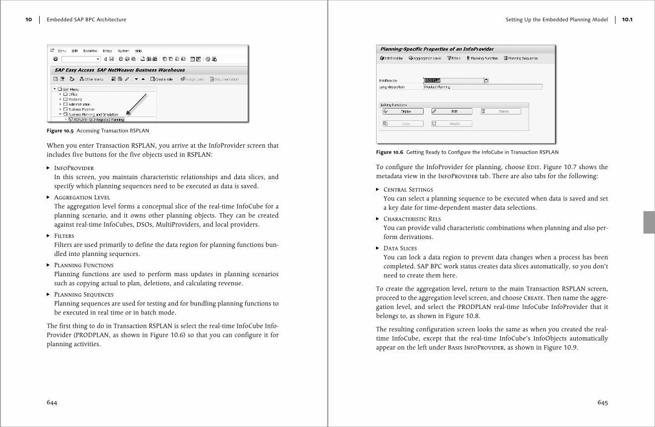
When you enter Transaction RSPLAN, you arrive at the InfoProvider screen thatincludes five buttons for the five objects used in RSPLAN:

� InfoProvider

In this screen, you maintain characteristic relationships and data slices, andspecify which planning sequences need to be executed as data is saved.

� Aggregation Level

The aggregation level forms a conceptual slice of the real-time InfoCube for aplanning scenario, and it owns other planning objects. They can be createdagainst real-time InfoCubes, DSOs, MultiProviders, and local providers.

� Filters

Filters are used primarily to define the data region for planning functions bun-dled into planning sequences.

� Planning Functions

Planning functions are used to perform mass updates in planning scenariossuch as copying actual to plan, deletions, and calculating revenue.

� Planning Sequences

Planning sequences are used for testing and for bundling planning functions tobe executed in real time or in batch mode.

The first thing to do in Transaction RSPLAN is select the real-time InfoCube Info-Provider (PRODPLAN, as shown in Figure 10.6) so that you can configure it forplanning activities.

Figure 10.5 Accessing Transaction RSPLAN


645

10.1

To configure the InfoProvider for planning, choose Edit. Figure 10.7 shows themetadata view in the InfoProvider tab. There are also tabs for the following:

� Central Settings

You can select a planning sequence to be executed when data is saved and seta key date for time-dependent master data selections.

� Characteristic Rels

You can provide valid characteristic combinations when planning and also per-form derivations.

� Data Slices

You can lock a data region to prevent data changes when a process has beencompleted. SAP BPC work status creates data slices automatically, so you don’tneed to create them here.

To create the aggregation level, return to the main Transaction RSPLAN screen,proceed to the aggregation level screen, and choose Create. Then name the aggre-gation level, and select the PRODPLAN real-time InfoCube InfoProvider that itbelongs to, as shown in Figure 10.8.

The resulting configuration screen looks the same as when you created the real-time InfoCube, except that the real-time InfoCube’s InfoObjects automaticallyappear on the left under Basis InfoProvider, as shown in Figure 10.9.

Figure 10.6 Getting Ready to Configure the InfoCube in Transaction RSPLAN


646

10

Figure 10.7 Viewing the InfoCube Metadata from Transaction RSPLAN

Figure 10.8 Creating an Aggregation Level

Figure 10.9 Creating an Aggregation Level


647

10.1

Based on the planning requirement, all you have to do is drag and drop theInfoObjects you need into the aggregation level on the right. As you can see inFigure 10.10, all of the InfoObjects in the real-time InfoCube have been selectedexcept for Posting Period, Material, Sales Unit (Unit is referenced to Quantity

so it needs to be included), Total Variable Costs, Sales Quantity, and Revenue.In other words, the planning activity is yearly planning so you don’t need Post-

ing Period; you’re planning by material group only, so you don’t need Material;

and so forth.

After the aggregation level is activated, you can use it to create planning func-tions.

10.1.3 Using a Copy Planning Function

IP provides quite a few planning functions, and being able to use them in embed-ded SAP BPC is a big advantage. We’ll be spending quite a bit of time going overthese in Chapter 13.

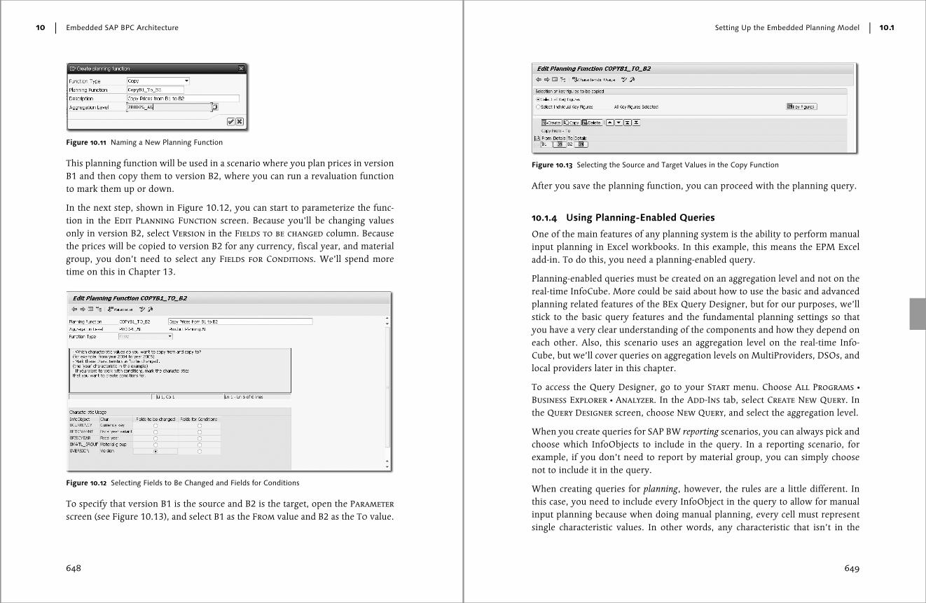
To create a planning function, you leave the Aggregation Level screen and moveinto the Planning Function screen. When you choose Create, you can select thefunction type, provide a name and description, and select the aggregation level,as shown in Figure 10.11.

Figure 10.10 The Completed Aggregation Level


648

10

This planning function will be used in a scenario where you plan prices in versionB1 and then copy them to version B2, where you can run a revaluation functionto mark them up or down.

In the next step, shown in Figure 10.12, you can start to parameterize the func-tion in the Edit Planning Function screen. Because you’ll be changing valuesonly in version B2, select Version in the Fields to be changed column. Becausethe prices will be copied to version B2 for any currency, fiscal year, and materialgroup, you don’t need to select any Fields for Conditions. We’ll spend moretime on this in Chapter 13.

To specify that version B1 is the source and B2 is the target, open the Parameter

screen (see Figure 10.13), and select B1 as the From value and B2 as the To value.

Figure 10.11 Naming a New Planning Function

Figure 10.12 Selecting Fields to Be Changed and Fields for Conditions


649

10.1

After you save the planning function, you can proceed with the planning query.

10.1.4 Using Planning-Enabled Queries

One of the main features of any planning system is the ability to perform manualinput planning in Excel workbooks. In this example, this means the EPM Exceladd-in. To do this, you need a planning-enabled query.

Planning-enabled queries must be created on an aggregation level and not on thereal-time InfoCube. More could be said about how to use the basic and advancedplanning related features of the BEx Query Designer, but for our purposes, we’llstick to the basic query features and the fundamental planning settings so thatyou have a very clear understanding of the components and how they depend oneach other. Also, this scenario uses an aggregation level on the real-time Info-Cube, but we’ll cover queries on aggregation levels on MultiProviders, DSOs, andlocal providers later in this chapter.

To access the Query Designer, go to your Start menu. Choose All Programs �

Business Explorer � Analyzer. In the Add-Ins tab, select Create New Query. Inthe Query Designer screen, choose New Query, and select the aggregation level.

When you create queries for SAP BW reporting scenarios, you can always pick andchoose which InfoObjects to include in the query. In a reporting scenario, forexample, if you don’t need to report by material group, you can simply choosenot to include it in the query.

When creating queries for planning, however, the rules are a little different. Inthis case, you need to include every InfoObject in the query to allow for manualinput planning because when doing manual planning, every cell must representsingle characteristic values. In other words, any characteristic that isn’t in the

Figure 10.13 Selecting the Source and Target Values in the Copy Function


650

10

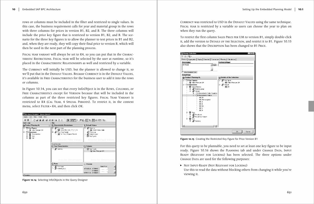
rows or columns must be included in the filter and restricted to single values. Inthis case, the business requirement calls for year and material group in the rowswith three columns for prices in version B1, B2, and B. The three columns willinclude the price key figure that is restricted to version B1, B2, and B. The sce-nario for the three key figures is to allow the planner to test prices in B1 and B2,and, when they are ready, they will copy their final price to version B, which willthen be used in the next part of the planning process.

Fiscal year variant will always be set to K4, so you can put that in the Charac-

teristic Restrictions. Fiscal year will be selected by the user at runtime, so it’splaced in the Characteristic Relationships as well and restricted by a variable.

The Currency will initially be USD, but the planner is allowed to change it, sowe’ll put that in the Default Values. Because Currency is in the Default Values,

it’s available in Free Characteristics for the business user to add it into the rowsor columns.

In Figure 10.14, you can see that every InfoObject is in the Rows, Columns, orFree Characteristics except for Version because that will be included in thecolumns as part of the three restricted key figures. Fiscal Year Variant isrestricted to K4 (Cal Year, 4 Special Periods). To restrict it, in the contextmenu, select Filter � K4, and then click OK.

Figure 10.14 Selecting InfoObjects in the Query Designer


651

10.1

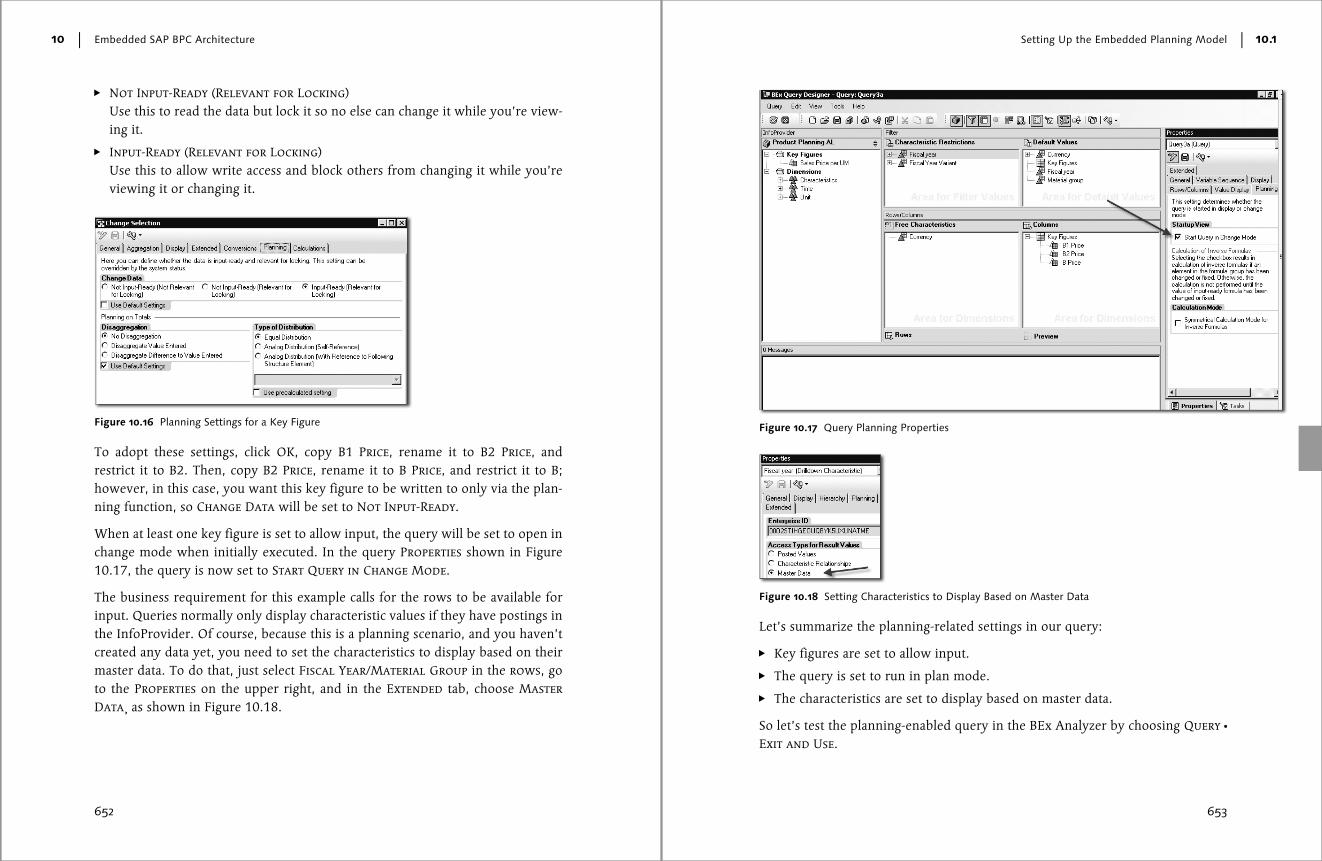
Currency was restricted to USD in the Default Values using the same technique.Fiscal year is restricted by a variable so users can choose the year to plan onwhen they run the query.

To restrict the first column Sales Price per UM to version B1, simply double-clickit, add the version to Details of the Selection, and restrict it to B1. Figure 10.15also shows that the Description has been changed to B1 Price.

For this query to be plannable, you need to set at least one key figure to be inputready. Figure 10.16 shows the Planning tab and under Change Data, Input

Ready (Relevant for Locking) has been selected. The three options underChange Data are used for the following purposes:

� Not Input-Ready (Not Relevant for Locking)Use this to read the data without blocking others from changing it while you’reviewing it.

Figure 10.15 Creating the Restricted Key Figure for Price Version B1


652

10

� Not Input-Ready (Relevant for Locking)Use this to read the data but lock it so no else can change it while you’re view-ing it.

� Input-Ready (Relevant for Locking)Use this to allow write access and block others from changing it while you’reviewing it or changing it.

To adopt these settings, click OK, copy B1 Price, rename it to B2 Price, andrestrict it to B2. Then, copy B2 Price, rename it to B Price, and restrict it to B;however, in this case, you want this key figure to be written to only via the plan-ning function, so Change Data will be set to Not Input-Ready.

When at least one key figure is set to allow input, the query will be set to open inchange mode when initially executed. In the query Properties shown in Figure10.17, the query is now set to Start Query in Change Mode.

The business requirement for this example calls for the rows to be available forinput. Queries normally only display characteristic values if they have postings inthe InfoProvider. Of course, because this is a planning scenario, and you haven’tcreated any data yet, you need to set the characteristics to display based on theirmaster data. To do that, just select Fiscal Year/Material Group in the rows, goto the Properties on the upper right, and in the Extended tab, choose Master

Data¸ as shown in Figure 10.18.

Figure 10.16 Planning Settings for a Key Figure


653

10.1

Let’s summarize the planning-related settings in our query:

� Key figures are set to allow input.

� The query is set to run in plan mode.

� The characteristics are set to display based on master data.

So let’s test the planning-enabled query in the BEx Analyzer by choosing Query �Exit and Use.

Figure 10.17 Query Planning Properties

Figure 10.18 Setting Characteristics to Display Based on Master Data


654

10

In the result set in Figure 10.19, B1 Price and B2 Price are available for inputbased on the light blue border in the data cells, whereas B Price isn’t and there-fore just has the black border.

In this case, the BEx Analyzer is only being used for testing because the ultimateUI will be the EPM add-in in Excel. To be able to use the EPM add-in, however,you first must create an embedded environment and a model.

10.1.5 Using Embedded SAP BPC Environments

If you have experience with standard SAP BPC, you know that when you’ve cre-ated environments, dimensions, and models in that version, the system gener-ated the corresponding InfoArea, characteristic, and real-time InfoCubes in SAPBW—all in their own namespace.

In contrast, embedded SAP BPC environments don’t have a correspondingInfoArea, and the characteristic and real-time InfoCubes aren’t created from theenvironment’s administration UI because they already exist in SAP BW with thenormal namespace. So why do you need an environment? In essence, the embed-ded SAP BPC environment provides a framework that allows you to use work sta-tus, BPFs, data audit, web reports/input forms, and the EPM add-in. After we’ve

Figure 10.19 The Query Default View in the BEx Analyzer


655

10.1

walked through the creation of an embedded environment, we’ll do some morecomparisons to standard environments.

In the administration screen, standard SAP BPC environments are still created bycopying from an existing environment. Embedded SAP BPC environments, onthe other hand, can only be created from scratch by choosing Create.

Because embedded SAP BPC environments don’t generate any SAP BW InfoAr-eas, characteristic, and InfoCubes, it doesn’t take very long to create them. To cre-ate an embedded environment, go to the web client, choose the currentlyconnected environment at the bottom of the screen, and then choose Manage �Manage all environments � Create.

In the resulting Create an Environment popup (see Figure 10.20), the Type

defaults to Unified (remember: embedded was initially referred to as “unified”).

After you input the Environment ID and Description and then choose Create

again, the new embedded environment is available for use.

In Figure 10.21, you can see the initial web client view with the Library screenselected. To do configuration in the web client, just go to Administration (seeFigure 10.22). In Administration, you can use the hypertext links to configureanything from Models to Data Audit.

You can now create an embedded model.

Figure 10.20 Creating an Embedded Environment


656

10

Figure 10.21 Embedded Web Client Library Screen

Figure 10.22 Embedded Web Client Administration Screen


657

10.1

10.1.6 Using SAP BPC Models

Before we discuss the configuration of embedded SAP BPC models, let’s talkabout what purpose they serve. Embedded SAP BPC models are used to selectInfoProviders to report or plan on. In addition, these models and their linkedInfoProviders contain the configuration for data profiles, work status, data audit,and BPFs.

So how many embedded models will you need? The answer always depends, but,in general, you’ll most often use one model for each InfoProvider. For example,in the simplest scenario, a real-time InfoCube is linked to one embedded SAP BPCmodel. If you’re using a MultiProvider, then you only need one embedded modelfor that as well. Conceptually, the model represents the type of reporting or plan-ning activity. If you need to do CapEx and HR planning, you’ll use a model forCapEx and another model for HR, and so forth.

Now that we’ve discussed the use case for embedded SAP BPC models, we can gointo the configuration steps. To create an embedded model, go to Administra-

tion and choose Models. Then the Create New Model dialog opens as shown inFigure 10.23.

After providing an ID and Description, select an InfoProvider, as shown in Figure10.24. When you go through the MultiProvider scenario later in this chapter,you’ll select several InfoProviders.

By choosing Next and then Create, you attach the model to an existing real-timeInfoCube. If you want to view the structure of the underlying real-time InfoCubefrom the web client, you can just select the model’s link; in the Structure tab,you can see the Characteristics and Key Figures as shown in Figure 10.25.

Figure 10.23 Creating an Embedded Model


658

10

Figure 10.24 Selecting the InfoProvider

Figure 10.25 Viewing the Characteristics and Key Figures of an Embedded Model


659

10.1

The Aggregation Levels and Related MultiProviders tabs display the structureof the related aggregation level and MultiProvider.

Note

Because the real-time InfoCube is compressed in SAP BW using process chains, theembedded web client doesn’t contain the model optimization option like the standardversion does.

Now that the embedded model is complete, you can configure data access pro-files, work status, and BPFs. It’s also available for web and EPM add-in planningand reporting.

10.1.7 Using the EPM Add-in Workbooks for Basic Planning Scenarios

The EPM add-in for Excel is, of course, the main user interface for planning andanalysis of embedded SAP BPC data. Building workbooks that include multipleEPM reports, drop-downs, buttons, and VBA for before and after events, and soon will take up a large portion of the development in an implementation.

Chapter 4 describes all of the basic and advanced features of the EPM add-in forstandard SAP BPC models. This chapter describes all of the basics when usingEPM add-in on embedded connections. In Chapter 11, we’ll get into the finerpoints of how the EPM add-in works when connected to embedded models.

To access the Excel EPM add-in, you can get there from the web client and use asystem-generated connection, or you can use the Start menu and create a newconnection. For this discussion of how to create a new connection for the embed-ded version, launch Excel from the Start menu, and go to the EPM tab. Of course,after you create a connection, it will be available the next time you log in.

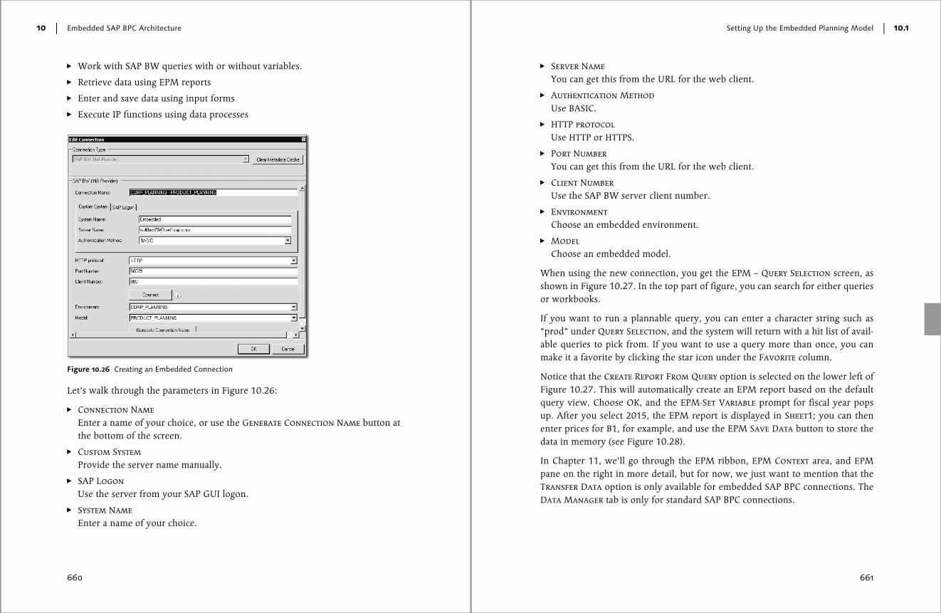
In the EPM tab, go to Report Actions, and choose Manage Connections. In theConnection Manager, create the connection with the parameters as shown inFigure 10.26.

If you’re familiar with standard SAP BPC, you’ll notice that there is a new connec-tion type: SAP BW (INA Provider), with INA standing for Information Access.This new connection type is required for embedded and provides the followingservices:


660

10

� Work with SAP BW queries with or without variables.

� Retrieve data using EPM reports

� Enter and save data using input forms

� Execute IP functions using data processes

Let’s walk through the parameters in Figure 10.26:

� Connection Name

Enter a name of your choice, or use the Generate Connection Name button atthe bottom of the screen.

� Custom System

Provide the server name manually.

� SAP Logon

Use the server from your SAP GUI logon.

� System Name

Enter a name of your choice.

Figure 10.26 Creating an Embedded Connection


661

10.1

� Server Name

You can get this from the URL for the web client.

� Authentication Method

Use BASIC.

� HTTP protocol

Use HTTP or HTTPS.

� Port Number

You can get this from the URL for the web client.

� Client Number

Use the SAP BW server client number.

� Environment

Choose an embedded environment.

� Model

Choose an embedded model.

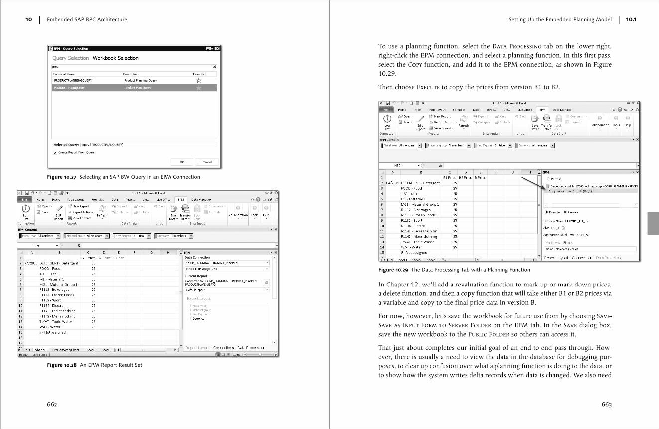
When using the new connection, you get the EPM – Query Selection screen, asshown in Figure 10.27. In the top part of figure, you can search for either queriesor workbooks.

If you want to run a plannable query, you can enter a character string such as“prod” under Query Selection, and the system will return with a hit list of avail-able queries to pick from. If you want to use a query more than once, you canmake it a favorite by clicking the star icon under the Favorite column.

Notice that the Create Report From Query option is selected on the lower left ofFigure 10.27. This will automatically create an EPM report based on the defaultquery view. Choose OK, and the EPM-Set Variable prompt for fiscal year popsup. After you select 2015, the EPM report is displayed in Sheet1; you can thenenter prices for B1, for example, and use the EPM Save Data button to store thedata in memory (see Figure 10.28).

In Chapter 11, we’ll go through the EPM ribbon, EPM Context area, and EPM

pane on the right in more detail, but for now, we just want to mention that theTransfer Data option is only available for embedded SAP BPC connections. TheData Manager tab is only for standard SAP BPC connections.


662

10

Figure 10.27 Selecting an SAP BW Query in an EPM Connection

Figure 10.28 An EPM Report Result Set


663

10.1

To use a planning function, select the Data Processing tab on the lower right,right-click the EPM connection, and select a planning function. In this first pass,select the Copy function, and add it to the EPM connection, as shown in Figure10.29.

Then choose Execute to copy the prices from version B1 to B2.

In Chapter 12, we’ll add a revaluation function to mark up or mark down prices,a delete function, and then a copy function that will take either B1 or B2 prices viaa variable and copy to the final price data in version B.

For now, however, let’s save the workbook for future use from by choosing Save�

Save as Input Form to Server Folder on the EPM tab. In the Save dialog box,save the new workbook to the Public Folder so others can access it.

That just about completes our initial goal of an end-to-end pass-through. How-ever, there is usually a need to view the data in the database for debugging pur-poses, to clear up confusion over what a planning function is doing to the data, orto show how the system writes delta records when data is changed. We also need

Figure 10.29 The Data Processing Tab with a Planning Function


664

10

to discuss compression because that plays a slightly different role now that we’reon SAP HANA.

10.1.8 Browsing and Compressing Data in SAP BW

To take a comprehensive approach, we also need to take a look at the data firstfrom SAP BW and then from the SAP HANA modeler.

But before we look at any data, let’s look at what data we’ve entered and saved inadvance for this test example:

� Enter “25” for JUC.

� Enter “25” for WAT, and save the data.

� Enter “35” for JUC.

� Enter “0” for WAT, and save the data.

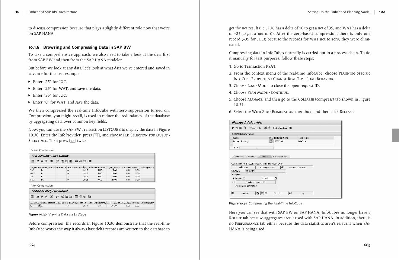
We then compressed the real-time InfoCube with zero suppression turned on.Compression, you might recall, is used to reduce the redundancy of the databaseby aggregating data over common key fields.

Now, you can use the SAP BW Transaction LISTCUBE to display the data in Figure10.30. Enter the InfoProvider, press (F8), and choose Fld Selection for Ouput �Select All. Then press (F8) twice.

Before compression, the records in Figure 10.30 demonstrate that the real-timeInfoCube works the way it always has: delta records are written to the database to

Figure 10.30 Viewing Data via ListCube

Before Compression:

After Compression:


665

10.1

get the net result (i.e., JUC has a delta of 10 to get a net of 35, and WAT has a deltaof –25 to get a net of 0). After the zero-based compression, there is only onerecord (–35 for JUC); because the records for WAT net to zero, they were elimi-nated.

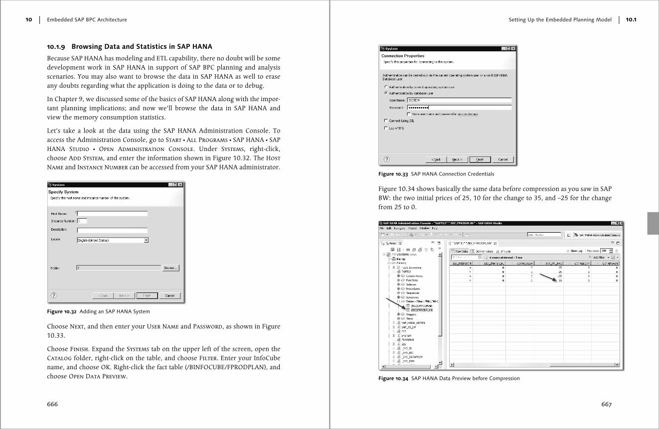
Compressing data in InfoCubes normally is carried out in a process chain. To doit manually for test purposes, follow these steps:

1. Go to Transaction RSA1.

2. From the context menu of the real-time InfoCube, choose Planning Specific

InfoCube Properties � Change Real-Time Load Behavior.

3. Choose Load Mode to close the open request ID.

4. Choose Plan Mode � Continue.

5. Choose Manage, and then go to the Collapse (compress) tab shown in Figure10.31.

6. Select the With Zero Elimination checkbox, and then click Release.

Here you can see that with SAP BW on SAP HANA, InfoCubes no longer have aRollup tab because aggregates aren’t used with SAP HANA. In addition, there isno Performance tab either because the data statistics aren’t relevant when SAPHANA is being used.

Figure 10.31 Compressing the Real-Time InfoCube


666

10

10.1.9 Browsing Data and Statistics in SAP HANA

Because SAP HANA has modeling and ETL capability, there no doubt will be somedevelopment work in SAP HANA in support of SAP BPC planning and analysisscenarios. You may also want to browse the data in SAP HANA as well to eraseany doubts regarding what the application is doing to the data or to debug.

In Chapter 9, we discussed some of the basics of SAP HANA along with the impor-tant planning implications; and now we’ll browse the data in SAP HANA andview the memory consumption statistics.

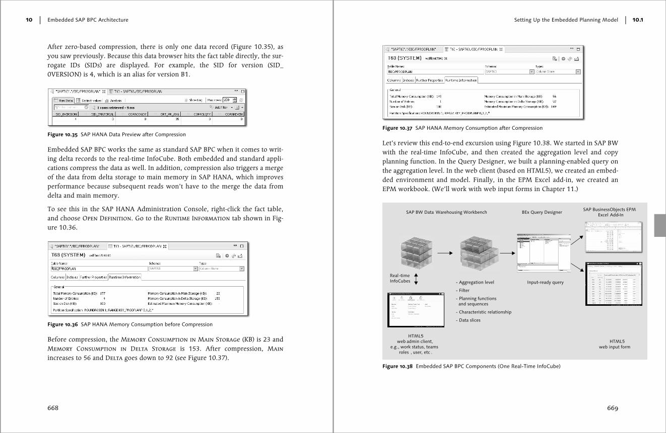
Let’s take a look at the data using the SAP HANA Administration Console. Toaccess the Administration Console, go to Start � All Programs � SAP HANA � SAP

HANA Studio � Open Administration Console. Under Systems, right-click,choose Add System, and enter the information shown in Figure 10.32. The Host

Name and Instance Number can be accessed from your SAP HANA administrator.

Choose Next, and then enter your User Name and Password, as shown in Figure10.33.

Choose Finish. Expand the Systems tab on the upper left of the screen, open theCatalog folder, right-click on the table, and choose Filter. Enter your InfoCubename, and choose OK. Right-click the fact table (/BINFOCUBE/FPRODPLAN), andchoose Open Data Preview.

Figure 10.32 Adding an SAP HANA System


667

10.1

Figure 10.34 shows basically the same data before compression as you saw in SAPBW: the two initial prices of 25, 10 for the change to 35, and –25 for the changefrom 25 to 0.

Figure 10.33 SAP HANA Connection Credentials

Figure 10.34 SAP HANA Data Preview before Compression


668

10

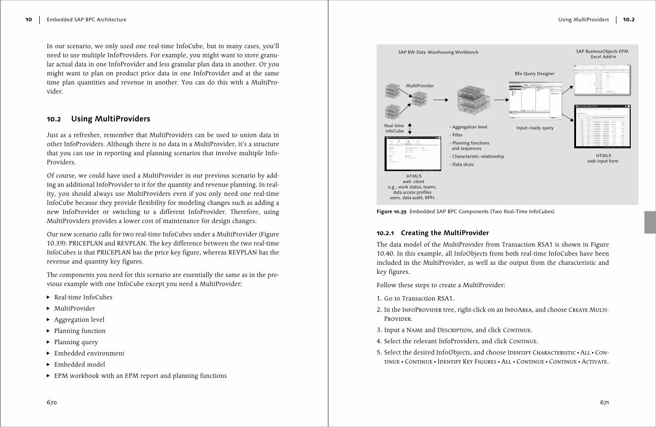
After zero-based compression, there is only one data record (Figure 10.35), asyou saw previously. Because this data browser hits the fact table directly, the sur-rogate IDs (SIDs) are displayed. For example, the SID for version (SID_0VERSION) is 4, which is an alias for version B1.

Embedded SAP BPC works the same as standard SAP BPC when it comes to writ-ing delta records to the real-time InfoCube. Both embedded and standard appli-cations compress the data as well. In addition, compression also triggers a mergeof the data from delta storage to main memory in SAP HANA, which improvesperformance because subsequent reads won’t have to the merge the data fromdelta and main memory.

To see this in the SAP HANA Administration Console, right-click the fact table,and choose Open Definition. Go to the Runtime Information tab shown in Fig-ure 10.36.

Before compression, the Memory Consumption in Main Storage (KB) is 23 andMemory Consumption in Delta Storage is 153. After compression, Main

increases to 56 and Delta goes down to 92 (see Figure 10.37).

Figure 10.35 SAP HANA Data Preview after Compression

Figure 10.36 SAP HANA Memory Consumption before Compression


669

10.1

Let’s review this end-to-end excursion using Figure 10.38. We started in SAP BWwith the real-time InfoCube, and then created the aggregation level and copyplanning function. In the Query Designer, we built a planning-enabled query onthe aggregation level. In the web client (based on HTML5), we created an embed-ded environment and model. Finally, in the EPM Excel add-in, we created anEPM workbook. (We’ll work with web input forms in Chapter 11.)

Figure 10.37 SAP HANA Memory Consumption after Compression

Figure 10.38 Embedded SAP BPC Components (One Real-Time InfoCube)

Input-ready query

BEx Query Designer

web input form

SAP BusinessObjects EPM Excel Add-InSAP BW Data Warehousing Workbench

Real -time InfoCubes - Aggregation level

- Filter

- Planning functions and sequences

- Characteristic relationship

- Data slices

HTML5 web admin client,

e.g., work status, teams roles , user, etc .

HTML5


670

10

In our scenario, we only used one real-time InfoCube, but in many cases, you’llneed to use multiple InfoProviders. For example, you might want to store granu-lar actual data in one InfoProvider and less granular plan data in another. Or youmight want to plan on product price data in one InfoProvider and at the sametime plan quantities and revenue in another. You can do this with a MultiPro-vider.

10.2 Using MultiProviders

Just as a refresher, remember that MultiProviders can be used to union data inother InfoProviders. Although there is no data in a MultiProvider, it’s a structurethat you can use in reporting and planning scenarios that involve multiple Info-Providers.

Of course, we could have used a MultiProvider in our previous scenario by add-ing an additional InfoProvider to it for the quantity and revenue planning. In real-ity, you should always use MultiProviders even if you only need one real-timeInfoCube because they provide flexibility for modeling changes such as adding anew InfoProvider or switching to a different InfoProvider. Therefore, usingMultiProviders provides a lower cost of maintenance for design changes.

Our new scenario calls for two real-time InfoCubes under a MultiProvider (Figure10.39): PRICEPLAN and REVPLAN. The key difference between the two real-timeInfoCubes is that PRICEPLAN has the price key figure, whereas REVPLAN has therevenue and quantity key figures.

The components you need for this scenario are essentially the same as in the pre-vious example with one InfoCube except you need a MultiProvider:

� Real-time InfoCubes

� MultiProvider


� Planning function

� Planning query

� Embedded environment

� Embedded model

� EPM workbook with an EPM report and planning functions

Using MultiProviders

671

10.2

10.2.1 Creating the MultiProvider

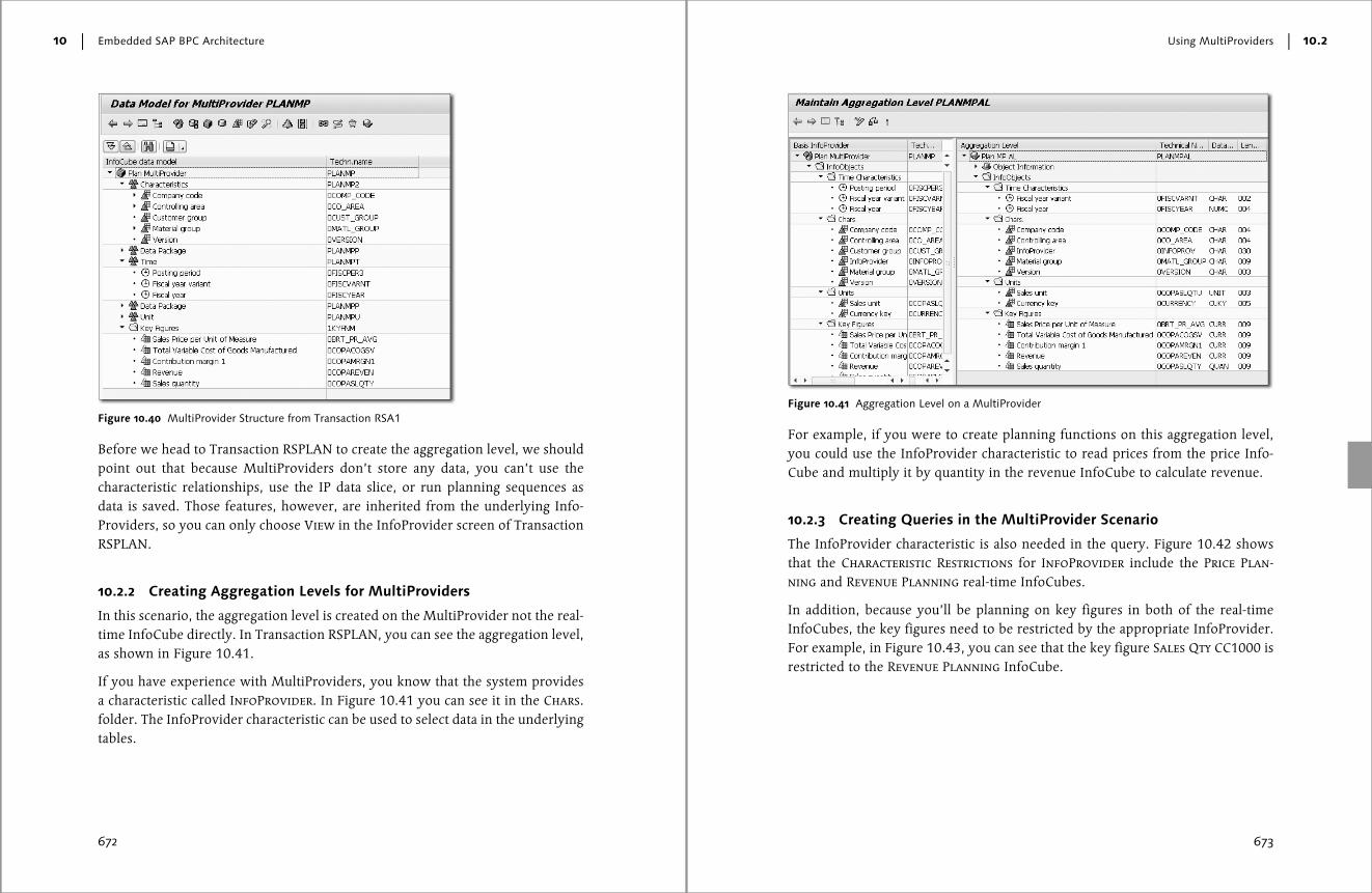
The data model of the MultiProvider from Transaction RSA1 is shown in Figure10.40. In this example, all InfoObjects from both real-time InfoCubes have beenincluded in the MultiProvider, as well as the output from the characteristic andkey figures.

Follow these steps to create a MultiProvider:

1. Go to Transaction RSA1.

2. In the InfoProvider tree, right-click on an InfoArea, and choose Create Multi-

Provider.

3. Input a Name and Description, and click Continue.

4. Select the relevant InfoProviders, and click Continue.

5. Select the desired InfoObjects, and choose Identify Characteristic � All � Con-

tinue � Continue � Identify Key Figures � All � Continue � Continue � Activate.

Figure 10.39 Embedded SAP BPC Components (Two Real-Time InfoCubes)

Input-ready query

BEx Query Designer

HTML5web input form

SAP BusinessObjects EPM Excel Add-In

SAP BW Data Warehousing Workbench

Real -time InfoCube

HTML5 web client

e.g., work status, teams, data access profiles

users, data audit, BPFs

MultiProvider

- Aggregation level

- Filter

- Planning functions and sequences

- Characteristic relationship

- Data slices


672

10

Before we head to Transaction RSPLAN to create the aggregation level, we shouldpoint out that because MultiProviders don’t store any data, you can’t use thecharacteristic relationships, use the IP data slice, or run planning sequences asdata is saved. Those features, however, are inherited from the underlying Info-Providers, so you can only choose View in the InfoProvider screen of TransactionRSPLAN.

10.2.2 Creating Aggregation Levels for MultiProviders

In this scenario, the aggregation level is created on the MultiProvider not the real-time InfoCube directly. In Transaction RSPLAN, you can see the aggregation level,as shown in Figure 10.41.

If you have experience with MultiProviders, you know that the system providesa characteristic called InfoProvider. In Figure 10.41 you can see it in the Chars.folder. The InfoProvider characteristic can be used to select data in the underlyingtables.

Figure 10.40 MultiProvider Structure from Transaction RSA1


673

10.2

For example, if you were to create planning functions on this aggregation level,you could use the InfoProvider characteristic to read prices from the price Info-Cube and multiply it by quantity in the revenue InfoCube to calculate revenue.

10.2.3 Creating Queries in the MultiProvider Scenario

The InfoProvider characteristic is also needed in the query. Figure 10.42 showsthat the Characteristic Restrictions for InfoProvider include the Price Plan-

ning and Revenue Planning real-time InfoCubes.

In addition, because you’ll be planning on key figures in both of the real-timeInfoCubes, the key figures need to be restricted by the appropriate InfoProvider.For example, in Figure 10.43, you can see that the key figure Sales Qty CC1000 isrestricted to the Revenue Planning InfoCube.

Figure 10.41 Aggregation Level on a MultiProvider


674

10

Figure 10.42 Query in the MultiProvider Scenario

Figure 10.43 Sales Quantity Key Figure Restricted to a Revenue Planning InfoCube


675

10.2

In contrast, the Price key figure is restricted to the Price Planning real-time Info-Cube, as shown in Figure 10.44.

To use the query in an EPM workbook, you need to create an embedded SAP BPCmodel.

10.2.4 Creating Embedded Models in the MultiProvider Scenario

To create an embedded model, go to the web client, choose Administration, andclick the Models link. Then just choose New, enter the ID and Description of themodel, and click Continue.

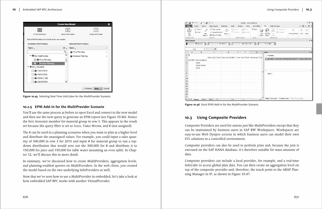
Next select the Price Planning and Revenue Planning InfoProviders shown inFigure 10.45. You may have expected that you would select the MultiProvider atthis point, but the SAP BPC features such as data audit, security, and work statusall relate to the InfoProviders themselves, which is why you select them and notthe MultiProvider.

After selecting the InfoCubes, choose Next, and then Finish. Now you can use theplanning-enabled query in the EPM add-in.

Figure 10.44 Price Key Figure Restricted to the Price Planning InfoCube


676

10

10.2.5 EPM Add-In for the MultiProvider Scenario

You’ll use the same process as before to open Excel and connect to the new modeland then use the new query to generate an EPM report (see Figure 10.46). Noticethe Not Assigned member for material group in row 3. This appears in the resultset because the query filter is set to Juice, Table Water, and # (not assigned).

The # can be used in a planning scenarios when you want to plan at a higher leveland distribute the unassigned values. For example, you could input a sales quan-tity of 300,000 in row 3 for 2015 and input # for material group to run a top-down distribution that would zero out the 300,000 for # and distribute it to150,000 for juice and 150,000 for table water (assuming an even split). In Chap-ter 12, we’ll discuss this in more detail.

In summary, we’ve discussed how to create MultiProviders, aggregation levels,and planning-enabled queries on MultiProviders. In the web client, you createdthe model based on the two underlying InfoProviders as well.

Now that we’ve seen how to use a MultiProvider in embedded, let’s take a look athow embedded SAP BPC works with another VirtualProvider.

Figure 10.45 Selecting Real-Time InfoCubes for the MultiProvider Scenario

Using Composite Providers

677

10.3

10.3 Using Composite Providers

Composite Providers are used for unions just like MultiProviders except that theycan be maintained by business users in SAP BW Workspaces. Workspaces areeasy-to-use Web Dynpro screens in which business users can model their ownETL solutions in a controlled environment.

Composite providers can also be used to perform joins and, because the join isexecuted on the SAP HANA database, it’s therefore suitable for mass amounts ofdata.

Composite providers can include a local provider, for example, and a real-timeInfoCube to access global plan data. You can then create an aggregation level ontop of the composite provider and, therefore, the touch point to the ABAP Plan-ning Manager in IP, as shown in Figure 10.47.

Figure 10.46 Excel EPM Add-In for the MultiProvider Scenario


678

10

Composite providers are a good example of how SAP HANA helps to provide datamodeling options for planning by making data consumption so much easier.

Now that we’ve seen how to use a MultiProvider and composite provider inembedded SAP BPC, let’s take a look at how to plan with DSOs.

10.4 Using DataStore Objects

Recall that real-time InfoCubes used with MultiProviders are the primary InfoPro-viders for embedded. DSOs can be used to fit more specialized scenarios such asfor price planning and comments. In addition, planning-enabled DSOs handledata changes a bit differently, so we’ll discuss that as well.

To use a DSO in embedded SAP BPC, you’ll need to create the following objects:

� Planning-enabled DSO


� Planning functions

� Planning query

Figure 10.47 Using a Composite Provider to Union Local and Global Data

Local provider Global plan data

Composite provider

Aggregation level

Union

Using DataStore Objects

679

10.4

� Embedded model

� Planning-enabled query


Of course, you would normally include the DSO in a MultiProvider and build theaggregation level on the MultiProvider in real-life scenarios.

10.4.1 Creating a Planning-Enabled DSO

To create a DSO, just go to Transaction RSA1, right-click on an InfoArea, andchoose Create DSO. Input a name and description, and use a template (here,tbw370s00) if you want to copy in a set of InfoObjects (see Figure 10.48).

After choosing Create, you can change the DataStore type (use the pencil icon)to Direct Update and check the box next to Planning Mode to make it plannable.These settings can’t be changed after there is data in the DSO.

As shown in Figure 10.49, we’ve moved all characteristic into the Key fields

folder, which is required to make it plannable.

If ever you need to expose the DSO data via an analytic view in SAP HANA, justcheck the box next to External SAP HANA View for reporting. The package inSAP HANA where the view is generated is set up in Transaction SPRO, and the

Figure 10.48 Creating a DSO from Transaction RSA1


680

10

SAP BW analysis authorizations are automatically created in the SAP HANA priv-ileges.

When the DSO is activated, the system creates an active table that will be used tostore the data (i.e., direct update DSOs don’t have three tables like standard DSOsdo, and planning-enabled DSOs can’t be loaded via SAP BW ETL).

In Transaction RSPLAN, you can use the characteristic relationships, data slices,and central settings (i.e., run planning sequences as data is saved) for planning-enabled DSOs.

10.4.2 Creating an Aggregation Level for a DSO

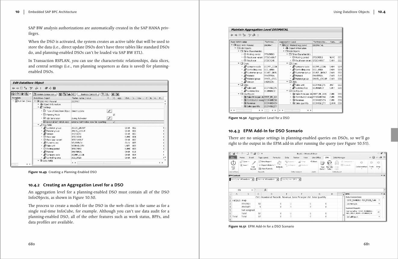
An aggregation level for a planning-enabled DSO must contain all of the DSOInfoObjects, as shown in Figure 10.50.

The process to create a model for the DSO in the web client is the same as for asingle real-time InfoCube, for example. Although you can’t use data audit for aplanning-enabled DSO, all of the other features such as work status, BPFs, anddata profiles are available.

Figure 10.49 Creating a Planning-Enabled DSO


681

10.4

10.4.3 EPM Add-In for DSO Scenario

There are no unique settings in planning-enabled queries on DSOs, so we’ll goright to the output in the EPM add-in after running the query (see Figure 10.51).

Figure 10.50 Aggregation Level for a DSO

Figure 10.51 EPM Add-In for a DSO Scenario


682

10

In general, the EPM add-in functions the same for a DSO as it does for a real-timeInfoCube or MultiProvider. However, here the delta buffer for a DSO works inoverwrite mode.

10.4.4 DSO Delta Buffer

For example, if you change the CM1 contribution margin for IPHONE4 from 12 to20, and IPHONE5 from 5 to 0, then the DSO only stores the latest data and not theoriginal value of 12 and the incremental change. After saving 20 and 0 from theEPM add-in, Figure 10.52 shows the database values.

10.4.5 DSO Price Planning

If you need to do price planning, consider using a planning-enabled DSO becauseit offers unique aggregation on parents. Generally speaking, you don’t usuallywant to aggregate prices because the total would be meaningless.

In plannable DSOs, if the children have different prices of 1.20, 1.30, and 1.50EUR, the parent (Water) value will display as NONEX in Figure 10.53. On theother hand, if all of the children of a parent have the same prices of 1.20 EUR,then that price (1.20 EUR) is displayed for the parent.

Let’s look at another use case for DSO price planning. If the product prices are dif-ferent, the planner can input a price for the parent (Water) and that price will beused for the individual products. For example, if you enter 25 for Water, then allthree water products would have a price of 25. In addition, if one of the waterproducts doesn’t have a price, then the price for water would display as a *.

Figure 10.52 The Data in a DSO after Saving Changes


683

10.4

10.4.6 DSO Comments

Aside from the price planning feature, you can also use plannable DSOs to storecomments. Comments can be used to record planning assumptions in the data-base, and then other users can run reports on the comments.

The architecture is shown in Figure 10.54. A planning-enabled DSO is included ina MultiProvider along with a real-time InfoCube. The real-time InfoCube containsthe transaction data, and the DSO is used to store the comments. The input formhas a separate column for comments and that column is a key figure in the DSOwith planning-enabled input.

The length of the comment can be up to 250 characters.

Figure 10.53 DSO Price Planning Example

If the values at leaf level have the same

value, the corresponding value will be

displayed at node level.

The following exception aggregations are

possible:

If the values at leaf level are different,

NONEX will be displayed at node level.

ProductGroup

Product Price

Water

Sparkling Water 0.5 l 1.20 €


Still Water 0.5 l 1.30 €

Product Group

Product Price

Water



Still Water 0.5 l 1.20 €

NONEX

1.20 €


684

10

10.5 Using Local Providers

The main use case for local providers is to provide a quick ad hoc reporting andplanning solution. Local providers are tables in SAP HANA that can be used with-out any corresponding SAP BW InfoObjects, so it’s potentially a low cost of devel-opment alternative that can be configured without any support from IT.

Local providers aren’t new with SAP BPC 10.1. They were originally offered aspart of SAP BW Workspaces, which is a small sandbox for business users to per-form ETL activities.

To use a local provider in a typical embedded SAP BPC planning scenario, you’llneed the following components:

� Local InfoProvider

� Embedded model

Figure 10.54 Embedded Comments with a DSO

DSO for comments. One comment per key

combina�on, comments only on base level, and

there is comment history

Aggrega�on Level: basis for the plan-enabled query

Product Group

Product Revenue Quantity Comment

Water 59000 45000 ?

Water Sparkling 0,5 18000 15000 Ok

Water Sparkling 1,0 15000 10000 Ok

Water Still 0,5 26000 20000 Good

Mul�Provider for data integra�on

InfoCube(s) for actualand plan data

Revenue and Quan�ty will be stored in an InfoCube.

Comment will be stored in a DSO object.

Using Local Providers

685

10.5

� Aggregation level (system-generated)

� Planning functions

� Planning query


10.5.1 Creating a Local Provider and Model

The use case for a local provider is based on a planning user who has a flat file ofactual data to upload into a database and then perform both manual input andautomatic planning via planning functions to further develop the result set. Inthis particular example, assume that you don’t want to use any existing InfoOb-jects as well. The flat file for the example has a header row and two rows of actualdata (see Figure 10.55).

To create the local provider, go to the web client, and choose InfoProviders �

Local Providers � New in the Administration screen. Enter a name and descrip-tion, and choose Next.

In the subsequent step (Upload Data File), you need to upload a flat file that isused to derive the structure of the resulting SAP HANA table and to provide theinitial result set. The flat file needs to have a .csv extension. As you can see in Fig-ure 10.56, these are the normal settings used in flat file loads to indicate if thereis a header row, data separators, decimal indicators, and so forth.

In the next step, Map InfoObjects, you can turn on data audit to track who madechanges to the data. This causes the system to add audit fields into the SAP HANAtable.

Figure 10.57 shows QTY and REV selected as the key figures. SAP HANA will cre-ate these as data fields.

Figure 10.55 Flat File for the Local Provider Scenario


686

10

In the Type column, select the data type for each field. For characteristics, youhave the following Type options:

� Character String with Leading Zeroes

� Date (saved as yyyymmdd)

� Time (saved as hhmmss)

� InfoObject

If you select InfoObject, you can select a characteristic and also choose whetherto use its conversion routine or not.

For the Key Figure fields, you have the following Type options:

� Integer

� Decimal

� Floating Point

� InfoObject

If you select InfoObject here, you can select a key figure.

In this example scenario, use Character String for characteristics and Integer forkey figures. While you’re creating the local provider, you can also create themodel on the fly. In the next step (Create Model), enter a model ID and descrip-tion (here, “LMODEL” as shown in Figure 10.58).

Finally, the system displays, among other things, the name of the aggregationlevel and query that it created automatically (see Figure 10.59). At the time ofwriting (fall 2014), the query must be created manually.

Figure 10.56 Upload a Flat File to Create a Local Provider


687

10.5

Figure 10.57 Turning on Data Audit and Selecting Data Types for a Local Provider

Figure 10.58 Create the Model for a Local Provider

Figure 10.59 Automatic Generation of an Aggregation Level for a Local Provider


688

10

10.5.2 An Aggregation Level for a Local Provider

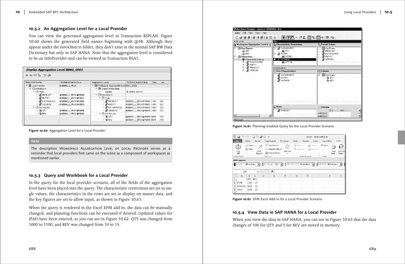
You can view the generated aggregation level in Transaction RSPLAN. Figure10.60 shows the generated field names beginning with @3B. Although theyappear under the InfoObjects folder, they don’t exist in the normal SAP BW DataDictionary but only in SAP HANA. Note that the aggregation level is consideredto be an InfoProvider and can be viewed in Transaction RSA1.

Note

The description Workspace Aggregation Level of Local Provider serves as areminder that local providers first came on the scene as a component of workspaces asmentioned earlier.

10.5.3 Query and Workbook for a Local Provider

In the query for the local provider scenario, all of the fields of the aggregationlevel have been placed into the query. The characteristic restrictions are set to sin-gle values, the characteristics in the rows are set to display on master data, andthe key figures are set to allow input, as shown in Figure 10.61.

When the query is rendered in the Excel EPM add-in, the data can be manuallychanged, and planning functions can be executed if desired. Updated values forIPAD have been entered, as you can see in Figure 10.62. QTY was changed from1000 to 1100, and REV was changed from 10 to 15.

Figure 10.60 Aggregation Level for a Local Provider


689

10.5

10.5.4 View Data in SAP HANA for a Local Provider

When you view the data in SAP HANA, you can see in Figure 10.63 that the datachanges of 100 for QTY and 5 for REV are stored in memory.

Figure 10.61 Planning-Enabled Query for the Local Provider Scenario

Figure 10.62 EPM Excel Add-In for a Local Provider Scenario


690

10

Because you turned on data audit, the SAP HANA table also includes four auditfields:

� User

� Data mode – PLAN

� Timestamp

� Source

See Chapter 13 for more information on data audit.

10.6 Summary

In this chapter, we touched on most of the major components for embedded SAPBPC architecture: real-time InfoCubes, MultiProviders, DSOs, composite provid-ers, and local providers. You now know the positioning to use for each one. Wemoved into the IP planning modeler in Transaction RSPLAN, and you saw how to

Figure 10.63 Viewing Local Provider Data in SAP HANA

Summary

691

10.6

create aggregation levels and planning functions. We created several planning-enabled queries and described the key planning settings. We then ran the queriesin the Excel EPM add-in, and you saw how to run IP functions from the data pro-cessing panel.

We’re now ready to take a look at how to perform reporting in embedded SAPBPC, starting with the BEx query in plan mode and moving into the EPM add-inin Excel and the web client.

7

Contents

Acknowledgments ............................................................................................ 17Introduction ..................................................................................................... 21

1 Planning and Consolidation at a Glance .................................. 37

1.1 Planning Basics ............................................................................ 381.2 Consolidation Basics .................................................................... 411.3 Summary ..................................................................................... 44

PART I Standard SAP PBC

2 The Fundamentals of Standard SAP BPC ................................. 47

2.1 System Architecture ..................................................................... 472.1.1 Microsoft Version ........................................................... 482.1.2 SAP NetWeaver Version .................................................. 50

2.2 Accessing the System ................................................................... 522.3 SAP Business Planning and Consolidation System ........................ 60

2.3.1 Library Objects ................................................................ 612.3.2 Component Toolbar ........................................................ 622.3.3 Support Toolbar .............................................................. 662.3.4 SAP Enterprise Performance Management (EPM)

Add-In ............................................................................ 692.4 SAP BPC Starter Kit Information .................................................. 77

2.4.1 IFRS Starter Kit ............................................................... 792.4.2 Other Starter Kits ............................................................ 80

2.5 Summary ..................................................................................... 81

3 Standard SAP BPC Architecture ............................................... 83

3.1 Terminology and Objects in SAP BPC ........................................... 833.2 Basic Data Modeling for SAP BPC ................................................ 87

3.2.1 Key Data Modeling Questions ......................................... 883.2.2 EnvironmentShell ............................................................ 943.2.3 Configuration/Copy of the EnvironmentShell ................... 97

3.3 Dimensions and Properties .......................................................... 100

Contents

8

3.3.1 Definition of Dimensions ................................................ 1013.3.2 Dimension Types ............................................................ 103

3.4 Creating a Dimension .................................................................. 1053.4.1 Time Dimension .............................................................. 1103.4.2 Category Dimension ........................................................ 1113.4.3 Account Dimension ........................................................ 1133.4.4 Entity Dimension ............................................................ 1163.4.5 Intercompany Dimension ................................................ 1183.4.6 Subtable/Flow Dimension ............................................... 1193.4.7 DataSource/AuditTrail Dimension ................................... 1203.4.8 Scope Dimension ............................................................ 1213.4.9 Rptcurrency Dimension ................................................... 1233.4.10 Inputcurrency Dimension ................................................ 1243.4.11 Additional Dimensions and Properties ............................ 124

3.5 Developing Components of the Dimensions ................................ 1263.5.1 Dimension Security ......................................................... 1263.5.2 Hierarchies in Dimensions ............................................... 1273.5.3 Custom Measure Formulas .............................................. 1283.5.4 Dimension Member Formulas ......................................... 1313.5.5 Owner Properties ............................................................ 1363.5.6 Reviewer Properties ........................................................ 137

3.6 Models ........................................................................................ 1383.6.1 Developing Models ......................................................... 1413.6.2 Creating Models ............................................................. 141

3.7 SAP BW Objects .......................................................................... 1473.7.1 Architecture of SAP BW Objects ..................................... 1483.7.2 SAP BW Objects Support for SAP BPC for

SAP NetWeaver .............................................................. 1483.7.3 SAP BW/SAP BPC InfoObjects ......................................... 1523.7.4 SAP BW/SAP BPC InfoCubes ........................................... 153

3.8 Summary ..................................................................................... 156

4 Reporting in Standard SAP BPC .............................................. 159

4.1 Report Considerations ................................................................. 1604.2 Introducing the EPM Add-In ....................................................... 170

4.2.1 Navigating in the EPM Add-In ........................................ 1764.2.2 Using the Context and Current Report Panes .................. 1784.2.3 Build a Basic Report ........................................................ 180

Contents

9

4.3 Using the EPM Ribbon ................................................................ 1874.3.1 Reports ........................................................................... 1884.3.2 Data Analysis .................................................................. 1944.3.3 Undo .............................................................................. 1974.3.4 Data Input ...................................................................... 1984.3.5 Collaboration .................................................................. 2074.3.6 Tools ............................................................................... 220

4.4 Using the EPM Add-In ................................................................. 2454.4.1 Report Editor and Report Selection ................................. 2464.4.2 Local Members ............................................................... 2544.4.3 Formatting of Reports ..................................................... 2584.4.4 Multi-Reports in a Workbook ......................................... 262

4.5 Excel Add-In Advanced Features .................................................. 2654.5.1 Asymmetric Reports ........................................................ 2654.5.2 EPM and FPMXL Functions ............................................. 267

4.6 PowerPoint and Word Documents in the EPM Add-In ................. 2704.7 Summary ..................................................................................... 273

5 Data Loading in Standard SAP BPC ......................................... 275

5.1 Basic Data Loading with SAP BPC ................................................ 2755.1.1 Data Manager ................................................................. 2765.1.2 SAP BW .......................................................................... 2855.1.3 Flat Files ......................................................................... 289

5.2 Loading Data in SAP BW ............................................................. 2935.2.1 Master Data, Text, and Hierarchies ................................. 2945.2.2 Transactional Data .......................................................... 304

5.3 Loading Data from SAP BW to SAP BPC ...................................... 3075.3.1 Master Data and Text ..................................................... 3085.3.2 Hierarchies ...................................................................... 3195.3.3 Transactional Data .......................................................... 329

5.4 Loading Data from a Flat File to SAP BPC .................................... 3405.4.1 Master Data and Hierarchy ............................................. 3415.4.2 Text ................................................................................ 3465.4.3 Transactional Data .......................................................... 348

5.5 Using the Data Manager .............................................................. 3555.5.1 Data Manager Configuration ........................................... 3565.5.2 Process Chains ................................................................ 362

5.6 Uploading Currency Exchange Rates for SAP BPC ......................... 366

Contents

10

5.6.1 Data Flow of Currency Exchange Rates to the Rate Model ............................................................... 368

5.6.2 Configuring SAP BW and SAP BPC for Exchange Rate Uploads .......................................................................... 369

5.7 Advanced Data Loading for SAP BW for SAP BPC ........................ 3765.7.1 Analysis of the DELTA INIT Process ................................. 3795.7.2 Setup of the SAP BW Process Chain to Execute the

SAP BPC Data Manager Package ..................................... 3845.8 Summary ..................................................................................... 392

6 Forecasting, Planning, and Budgeting in Standard SAP BPC ... 395

6.1 Basic Planning, Forecasting, and Budgeting ................................. 3956.1.1 Driver-Based Approach ................................................... 4026.1.2 Top-Down and Bottom-Up Approaches .......................... 402

6.2 Script Logic in SAP BPC ............................................................... 4036.2.1 Worksheet Logic ............................................................. 4056.2.2 Dimension Member Logic ............................................... 4066.2.3 Standard Script Logic Prompts for SAP BPC ..................... 4066.2.4 Use of Script Logic in the Planning Process ...................... 4206.2.5 Allocation Script Logic .................................................... 4346.2.6 Script Logic in the Automation of Data Loading .............. 4356.2.7 BAdIs and the ABAP Program ......................................... 438

6.3 Generic Planning Process ............................................................. 4426.3.1 Initial Planned Data ........................................................ 4426.3.2 Copy Process .................................................................. 4436.3.3 Executing Calculations .................................................... 4446.3.4 Top-Down Planning ........................................................ 4456.3.5 Bottom-Up Planning ....................................................... 4546.3.6 Data Transfer Process ...................................................... 454

6.4 Summary ..................................................................................... 455

7 Consolidation in Standard SAP BPC ........................................ 457

7.1 Basic Consolidation ..................................................................... 4577.1.1 What Consolidation Is All About ..................................... 4577.1.2 Performing Consolidations with SAP BPC ........................ 4597.1.3 Introducing Business Rules .............................................. 461

Contents

11

7.2 Ownership Data and Elimination Methods .................................. 4647.2.1 The Ownership Process ................................................... 4647.2.2 Setting Up Ownership Data ............................................ 4667.2.3 The Purchase Method Concept ....................................... 4717.2.4 The Proportional and Equity Method Concepts ............... 472

7.3 Setting Up Journal Entries ............................................................ 4737.3.1 The Business Scenario for Using Journal Entries ............... 4737.3.2 Creating Journal Templates ............................................. 4737.3.3 Controlling Journal Activity ............................................. 4757.3.4 Creating Journal Entries .................................................. 476

7.4 Setting Up and Executing Consolidation Tasks ............................. 4777.4.1 Balance Carry Forward .................................................... 4787.4.2 Reclassification ............................................................... 4837.4.3 Currency Translation for Consolidation ............................ 4877.4.4 Purchase Method Elimination ......................................... 4967.4.5 Proportional Method Elimination .................................... 5077.4.6 Equity Method Elimination ............................................. 5117.4.7 Ownership Elimination .................................................... 5137.4.8 Intercompany Matching .................................................. 5207.4.9 Intercompany Elimination ............................................... 5257.4.10 US Eliminations ............................................................... 528

7.5 Setting Up Balancing Script Logic for Consolidation ..................... 5327.6 Setting Up and Executing Equity Pick Up ..................................... 536

7.6.1 Prerequisites for Using Equity Pick Up for Banking .......... 5367.6.2 Equity Pick Up Business Rule ........................................... 5377.6.3 Equity Pick Up Monitor ................................................... 541

7.7 The Consolidation Monitor .......................................................... 5437.7.1 Prerequisites to Use the Consolidation Monitor .............. 5437.7.2 Using the Consolidation Monitor .................................... 543

7.8 Summary ..................................................................................... 548

8 Managing the Standard SAP BPC Process ............................... 549

8.1 Security ....................................................................................... 5498.1.1 Users .............................................................................. 5528.1.2 Teams ............................................................................. 5558.1.3 Task Profiles .................................................................... 5578.1.4 Data Access Profiles ........................................................ 5598.1.5 Security in the EPM Add-In ............................................. 563

Contents

12

8.2 Work Status ................................................................................. 5648.2.1 Configuration of Work Status .......................................... 5648.2.2 Reporting and Managing Work Status ............................. 568

8.3 Controls ...................................................................................... 5718.3.1 Configuration .................................................................. 5718.3.2 Control Monitor .............................................................. 578

8.4 System Reporting ........................................................................ 5808.4.1 System Reporting ............................................................ 5848.4.2 Audit Tables Reports ....................................................... 591

8.5 Transports ................................................................................... 5968.6 Summary ..................................................................................... 605

PART II Embedded SAP BPC

9 The Fundamentals of Embedded SAP BPC .............................. 609

9.1 The Evolution of SAP BPC ............................................................ 6099.2 A Primer on SAP HANA ............................................................... 6189.3 Comparing Standard and Embedded Features .............................. 6249.4 Strategy for Conversion ................................................................ 631

9.4.1 From IP with PAK Turned On .......................................... 6319.4.2 From SAP Business Planning and Simulation ................... 6329.4.3 From SAP BPC 7.x ........................................................... 6339.4.4 From SAP BPC 10.0 without SAP HANA ......................... 6349.4.5 Hybrid/Mixed Scenarios .................................................. 6359.4.6 New Customer with Business Ownership Focus ............... 6359.4.7 New Customer with EDW Integration Focus ................... 636

9.5 Deployment Options ................................................................... 6369.6 Summary ..................................................................................... 638

10 Embedded SAP BPC Architecture ............................................ 639

10.1 Setting Up the Embedded Planning Model .................................. 63910.1.1 Using Real-Time InfoCubes ............................................. 64010.1.2 Using Aggregation Levels ................................................ 64310.1.3 Using a Copy Planning Function ...................................... 64710.1.4 Using Planning-Enabled Queries ..................................... 64910.1.5 Using Embedded SAP BPC Environments ........................ 65410.1.6 Using SAP BPC Models ................................................... 657

Contents

13

10.1.7 Using the EPM Add-in Workbooks for Basic Planning Scenarios ........................................................................ 659

10.1.8 Browsing and Compressing Data in SAP BW ................... 66410.1.9 Browsing Data and Statistics in SAP HANA ..................... 666

10.2 Using MultiProviders ................................................................... 67010.2.1 Creating the MultiProvider .............................................. 67110.2.2 Creating Aggregation Levels for MultiProviders ............... 67210.2.3 Creating Queries in the MultiProvider Scenario ............... 67310.2.4 Creating Embedded Models in the MultiProvider

Scenario .......................................................................... 67510.2.5 EPM Add-In for the MultiProvider Scenario .................... 676

10.3 Using Composite Providers .......................................................... 67710.4 Using DataStore Objects .............................................................. 678

10.4.1 Creating a Planning-Enabled DSO ................................... 67910.4.2 Creating an Aggregation Level for a DSO ........................ 68010.4.3 EPM Add-In for DSO Scenario ........................................ 68110.4.4 DSO Delta Buffer ............................................................ 68210.4.5 DSO Price Planning ......................................................... 68210.4.6 DSO Comments .............................................................. 683

10.5 Using Local Providers .................................................................. 68410.5.1 Creating a Local Provider and Model ............................... 68510.5.2 An Aggregation Level for a Local Provider ....................... 68810.5.3 Query and Workbook for a Local Provider ....................... 68810.5.4 View Data in SAP HANA for a Local Provider .................. 689

10.6 Summary ..................................................................................... 690

11 Reporting with Embedded SAP BPC ........................................ 693

11.1 System Architecture Review ........................................................ 69411.2 Web Client Reporting .................................................................. 69511.3 EPM Add-In in the Embedded Model .......................................... 702

11.3.1 EPM Features .................................................................. 70411.3.2 Using EPM ...................................................................... 706

11.4 Comparing the EPM Add-In for Standard and Embedded ............ 71111.5 EPM Add-In for SAP HANA Data ................................................. 71211.6 SAP BusinessObjects Analysis, Edition for Microsoft Office .......... 71611.7 Summary ..................................................................................... 720

Contents

14

12 Forecasting, Planning, and Budgeting in Embedded SAP BPC ................................................................................... 721

12.1 Standard IP Planning Functions ................................................... 72212.1.1 The Copy Function .......................................................... 72212.1.2 The Revaluation Function ................................................ 72412.1.3 The Delete Function ....................................................... 72512.1.4 The Repost Function ....................................................... 725

12.2 Executing Planning Functions from Excel ..................................... 72612.2.1 Data Processing Tab ........................................................ 72612.2.2 Pushbuttons .................................................................... 728

12.3 Disaggregation and Inverse Formulas ........................................... 73012.3.1 Disaggregation ................................................................ 73112.3.2 Inverse Formulas ............................................................. 733

12.4 Planning Filters and Planning Sequences ...................................... 73612.4.1 Planning Filters ............................................................... 73612.4.2 Planning Sequences ........................................................ 738

12.5 FOX Formulas .............................................................................. 74112.5.1 Create a Driver-Based Formula ........................................ 74212.5.2 Create a FOX Formula with a Condition .......................... 74612.5.3 Create a Formula to Calculate Revenue Based on the

Prior Year ........................................................................ 74712.5.4 Create a Formula with a Loop ......................................... 749

12.6 Characteristic Relationships ......................................................... 75112.6.1 Combination Checking .................................................... 75112.6.2 Characteristic Derivation ................................................. 754

12.7 Advanced Planning Functions ...................................................... 75612.7.1 Currency Translation ....................................................... 75612.7.2 Unit of Measure Conversion ............................................ 76112.7.3 Top-Down Distribution ................................................... 76512.7.4 Distribution with Keys .................................................... 76912.7.5 Deletion of Invalid Combinations .................................... 77012.7.6 Repost on Basis of Characteristic Relationships ................ 77212.7.7 Generate Combinations .................................................. 77312.7.8 Custom Planning Functions ............................................. 775

12.8 Summary ..................................................................................... 779

Contents

15

13 Managing the Embedded SAP BPC Process ............................ 781

13.1 Security ....................................................................................... 78113.1.1 Users .............................................................................. 78213.1.2 Teams ............................................................................. 78413.1.3 Data Access Profiles ........................................................ 78413.1.4 Matrix Security ................................................................ 79113.1.5 Authorization Objects ..................................................... 792

13.2 Work Status ................................................................................. 79413.2.1 Configuration .................................................................. 79513.2.2 Using Work Status .......................................................... 80013.2.3 Reporting ........................................................................ 801

13.3 Data Audit ................................................................................... 80413.3.1 Configuration .................................................................. 80413.3.2 Using Embedded Data Audit ........................................... 807

13.4 Transports ................................................................................... 81113.5 Summary ..................................................................................... 813

14 Migrating to SAP BPC 10.1 ...................................................... 815

14.1 SAP BPC 7.5 to Standard SAP BPC 10.1 ....................................... 81714.2 SAP BPC 10.0 to Standard SAP BPC 10.1 ..................................... 82214.3 Integration Planning to Embedded SAP BPC 10.1 ........................ 82414.4 SAP BPC 10.0 to Embedded SAP BPC .......................................... 82514.5 SAP BPC 10.0 to Mixed Standard/Embedded SAP BPC 10.1 ........ 82614.6 Summary ..................................................................................... 826

The Authors ..................................................................................................... 827Index ................................................................................................................ 829

829

Index

$INFOCUBE, 75%APPLICATION%, 432%APPSET%, 432%ENTITY_DIM%, 362%TIME_SET%, 418%YEAR%, 432*ADD /*ENDADD, 432*ADD/*ENDADD, 410*COL(X), 349*COMMIT, 411, 417, 423*DESTINATION_APP, 415*ENDALLOCATION, 435*ENDWHEN, 414*INCLUDE, 411*LOOKUP, 416*LOOKUP {MODEL}, 416*MVAL, 331*NEWCOL, 331*NEWCOL(X), 349*REC, 412, 428, 429*RUNALLOCATION, 434*SELECT, 413, 431*WHEN, 413*WHEN/*ENDWHEN, 413*WHEN/*IS/*ENDWHEN, 429*XDIM_ADDMEMBERSET, 416, 428*XDIM_FILTER, 428*XDIM_MEMBERSET, 412, 415, 422, 427.NET, 48, 50/CPMB/, 55, 154, 364/CPMB/LOAD_DELTA_IP, 3360GL_ACCOUNT, 300, 3190GLACCEXT, 3770TCAACTVT, 7860TCAIPROV, 7860TCAVALID, 786501, 281

A

ABAP code, 293ABAP program, 438

ABAP/BAdI, 420ACCOUNT, 108Account and key figure-based InfoCubes, 615Account dimension, 113Account-based calculations, 463Account-based view, 85ACCTYPES, 105, 115Activate Local Member Recognition option,

230, 254, 255Activate Member Recognition checkbox, 180Activate Member Recognition option, 230Activate Metadata Cache option, 238Active cell, 204Activities, 571, 585

audit, 581, 582monitor, 569report, 585

Add Comment option, 204Add Conversion Sheet option, 284Add Data Link option, 222, 223Add dimension, 164Add Member Link option, 222Add Report Link option, 222Add/Remove button, 576Adding comments, 422Admin console, 816Admin Package option, 352ADMINISTRATION, 64Administration, 436Administration activity audit, 582Adobe Flex web, 612Advanced, 190Aggregate overwrite option, 337Aggregation level, 616, 639, 643, 647, 649,

669, 670, 672, 677, 678, 680, 685, 686, 688, 693, 694, 710create, 643, 646

Allocation, 395, 434, 456, 621Allocation Script Logic, 434ALLOCATION.LGF, 409Allow Member Formulas checkbox, 109AMOUNTDECIMALPOINT, 311

Index

830

Analog distribution, 732with reference, 732

Analytic view, 623Answer Prompt field, 388Append, 357Append option, 337APPROVALSTATUSMAIL, 568APPROVALSTATUSMSG, 568Assign dimension name, 327Assignment of the transport, 601Assignments of the control set, 576Asymmetric report, 173, 265, 266Attribute, 86, 294

SAP BW, 281Attribute List tab, 316Attribute view, 623Audit, 584Audit data, 584Audit process component, 596Audit report, 584Audit security, 587Audit tables, 581, 591Audit tables reports, 591Authorization, 636Authorization objects, 792Authorization relevant, 785Automated data processing, 435Automatic Refresh on Context Changes

option, 237

B

Backup, 817, 818, 819, 823BAdI, 420, 438, 439, 440, 455Balance carry forward, 460, 478

business scenario, 478Balancing logic

business scenario, 532Balancing Script Logic, 532Basic InfoCube, 162BEx Analyzer, 609, 610, 653, 654, 803BEx queries, 826Block number, 741Body, 427Body/code, 426, 428Book Publication option, 207, 211, 220

Bottom-up planning, 395, 402, 454, 456BPS, 609, 632Budget SAP BPC model, 349Budgeting, 396Business ownership, 635Business process flow (BPF), 137, 324, 584

activity audit, 582activity report, 586creation, 581reporting, 585

Business rule, 461, 581configuration, 464methods, 462

BW Implementation Guide, 57By Percentage, 200

C

CALCACCOUNT.LGF, 409Calculate Parents in Hierarchies option, 233Calculated key figure, 187Calculated Members option, 258Calculation view, 623Calling the Script Logic, 427Cancel execution, 182Cancel option, 182CapEx, 81, 657Capital Expenditure Planning Starter Kit, 80Capital expenditure E, 397Cases sold, 349Category, 367, 398Category dimension, 111Central settings, 645Central unit of measure, 764CFSV, 328Change Connection option, 189, 245Change status, 100Change Status button, 603Change Work Status option, 203, 568Changed Members option, 258Characteristic, 86, 294, 640, 642, 652, 657,

658, 686, 688derivation, 751, 754relationships, 621, 645, 722, 751restrictions, 650SAP BW, 281

Index

831

Characteristic (Cont.)values, 86

Children option, 195, 230Clear, 277, 357Clear Data Data Manager package, 423Clear datavalues, 338Clear MetaData Cache Frequency option, 238Clear Metadata Cache option, 244CMS account, 821Collaboration, 207Collapse option, 195Collection, 220, 600Column axis, 184COM add-in, 178Combination checking, 751Command Display Options screen, 242Comments, 203, 567, 588, 631, 702, 705, 711,

720, 824saving, 198

Comments options, 231Commit, 426Components of security, 781Composite Providers, 677Compound characteristic, 318Compound InfoObject, 318, 328, 376Compounding, 153, 162Compression, 664, 667, 668, 669Concatenation of the compound, 328Conditional logic, 433Configuration of work status, 564Configuration parameters, 58Consistent security process, 562Consolidation, 41, 160, 457, 611Consolidation Central component, 51Consolidation model, 95, 329, 359Consolidation Monitor, 51, 63, 64, 461, 543Consolidation task, 477CONSOLIDATION.LGF, 409Constants, 359Constants in the logic file, 410Context and current report panes, 178Context Favorite option, 204Context Options feature, 234Control component, 579Control data for work status, 565Control Monitor, 576, 578

Control set, 575CONTROL_LEVEL, 571Controlled by section, 566Controller by Permitted Data Entry Methods

section, 567Controls, 571, 577, 578, 579Controls configuration, 572Controls Monitor, 63, 579Conversion, 282, 310Conversion file, 279, 289, 308, 321

options, 283Conversion to SAP BPC 10.0, 631Copy, 277, 455, 721

function, 722, 723process chain, 359, 443tasks, 359

COPY Data Manager package, 423Copy report, 191COPY_OPENING.LGF, 409Cost center, 85CPM software components, 825Create a DSO, 679Create a model, 141Create a MultiProvider, 671Create a query, 673Create embedded connection, 660Create portion, 163Creating journal entries, 476Creating journal templates, 473CREDITPOSITIVE, 312CSV file, 342CSV format, 290CTRL_CURRENCY_NOT_LC, 572Currency, 721, 756, 757, 759Currency exchange rate, 367Currency keyword, 490Currency translation, 460, 463, 487, 756

business scenario, 487function, 761type, 759

Current Report pane, 178, 180, 183Current Report screen, 184Custom context, 204Custom Expand option, 195, 230Custom measure formula, 128Custom member, 257

Index

832

Custom Member Default Format option, 258Custom planning functions, 775Customer dimension with properties, 342

D

Data, 315Data access profile, 550, 551, 552, 555, 556,

559, 561, 587, 659, 784, 788Data analysis, 194Data audit, 581, 582, 590, 616, 631, 655, 687,

804, 822, 824, 825configuration, 583information, 581process, 582purge, 584

Data changes, 588, 589, 807Data collection component, 362Data connection, 263, 264Data flow, 276, 286Data flow of currency exchange, 368Data input options, 198, 230Data Language option, 239Data Link Symbol Color option, 239Data loading in SAP BW, 293Data Manager, 270, 276, 277, 291, 310, 355,

356, 408, 705, 711, 720, 819configuration, 356upload dialog, 279

Data Manager Group, 279, 342options, 279, 291

Data Manager Import, 592Data Manager package, 379, 423, 440Data mapping, 308Data modeling, 93Data preview, 291Data Preview option, 279, 342Data processing, 705, 711, 717, 726, 727, 728,

761Data Processing tab, 712, 726Data profile, 618, 631Data slice, 645Data transfer, 395Data transfer process (DTP), 304, 598Data type, 314, 333, 749Data validation, 460

Database migration, 825Database procedure, 778DataSource, 286, 287, 294, 296, 297, 298,

304, 379, 598DataSource Object, 639, 678, 680, 682, 683,

702, 712DataSource/AuditTrail dimension, 120DataStore object (DSO), 287, 304, 368Default values, 650DEFAULT.LGF, 407, 408Defer Layout Update option, 184, 186Delete function, 722, 725Delete invalid characteristic combinations,

751Delete invalid combinations, 770Delete reports, 191Delimited or Fixed Width options, 291Delimiter, 311Delta buffer, 682DELTA INIT package, 379Delta initialization, 379Delta loading process, 281Delta Update option, 305Delta updating, 296Denied, 560, 561Deployment options, 631Depreciation calculation, 444Derivation, 752Descendant option, 195, 230DETAILS, 339Dimension, 84, 143, 211, 275, 294, 397

SAP BPC, 281Dimension formulas, 131Dimension member formula, 404, 623Dimension member logic, 406Dimension Member/Property Formatting

section, 258, 262Dimension security, 126Dimension type, 103Dimension/field, 381Disaggregation, 619, 721, 731, 733, 765, 769Display component, 355Display Disaggregation Warning option, 240Display EPM Context Bar option, 237Display input template, 739Display Local Connections option, 239

Index

833

Display MDX option, 243Distribution, 207, 211, 721, 731, 768

by key, 765Collect option, 208Distribute option, 207non-assigned, 766Now option, 215option, 211template, 214with keys, 769, 770with reference, 765, 766, 769

Do Not Load Members at Connection, 76Do Not Load Members at Connection

checkbox, 174Do not Store Connection option, 169Document type, 209Documents feature, 66Documents option, 97Download Center option, 68Download Data option, 279Drill Through option, 221, 222, 227Drill-through, 227, 705, 711, 720Driver, 396Driver-based formula, 742Driver-based planning, 402Drivers and rates, 138Dynamic Package Script, 357

E

Edit E-Mail Notification Settings dialog box, 567

Edit layout, 164Edit report, 245Edit Report and New Report, 192Edit Report option, 246, 271EDW BW Integration, 624Elimination methods, 464Eliminations and adjustments, 463Eliminations and adjustments rule screen

Details tab, 502General tab, 500

Email notification, 567Embedded component, 669Embedded connections, 659, 660Embedded data model, 657, 684

Embedded environment, 640, 654, 670Embedded planning model, 639, 640, 670,

679Embedded web client, 659Embedded web client administration, 656Enable Controls by Model parameters, 572Enable Double-Click option, 182, 237Enable work status, 795Enable Work Status by Model section, 565ENABLE_FIXED_CUBENAME, 59Enhancement spot, 439

UJ_CUSTOM_LOGIC, 439Enterprise Cloud, 636Entity dimension, 116Environment, 86, 88, 99, 661

connection, 106offline, 603option, 68

EnvironmentShell, 53, 57, 83, 84, 89, 94, 97, 408alterations, 95

EPM – Distribution Template screen, 212EPM 10.1, 69, 170EPM add-in, 159, 160, 163, 166, 170, 172,

176, 183, 188, 265, 267, 404, 405, 436, 563, 568, 592, 611, 612, 613, 618, 632, 633, 639, 654, 659, 676, 677, 681, 682, 688description, 270formatting parameters, 261formatting sheet, 168, 260frontend, 551functions, 225, 274reporting tool, 172ribbon, 187, 188, 190, 193, 201, 661

EPM context menu, 178, 179, 180, 185EPM Office add-in for Excel, 277, 310EPM Office Add-in options, 68EPM SAP Template, 168EPM Workbook, 640, 670, 679EPM Worksheet option, 231EPMAddInAutomation, 730EPMComparison, 269EPMFormattingSheet, 260EPMMemberDesc, 269Equal distribution, 732, 767

Index

834

Equity method, 42business scenario, 511elimination, 511

Equity Pick Up, 536business rule, 537for banking, 536

Equity Pick Up Monitor, 541Essbase, 183EvDRE, 169, 183, 221, 822

Migration option, 245templates, 634

Excel add-in advanced features, 265Exchange rate, 289, 290

type, 371Exclude option, 196Excluded Members tab, 247, 254Execute planning sequence, 739Execute Step with Trace option, 745ExecuteDataProcess, 728Expand option, 195Expand Options feature, 230Expand/Collapse on Single Member option,

237Expand/Collapse options, 195External column, 283External formatting, 326External option, 323Extraction tab, 296

F

Favorites feature, 62Field to be changed, 724, 747, 749, 758, 763,

766Fields for conditions, 723Filter, 644Filtering, 252Filtering tab, 247, 250Filters, 721, 726Finance model, 167Financial expenses, 397Financial Information Management, 69Financial model, 400Find Comments option, 204, 205Finish editing, 166FireFly, 695, 702, 706

First consolidation entries, 472Fixed and variable fields, 214Fixed data format, 298Flash Objects option, 243Flat file, 275, 291, 317, 340Flow, 119FOREACH, 750Forecasting, 396FORMAT, 311Format, 164, 315Formatting of reports, 258Formatting sheet, 260Formatting tab, 232Formula column, 283, 284, 331Formula name field, 129FOX, 621, 721FOX formula, 741FOX formula with a condition, 746FPMXL, 267

FPMXLClient, 168, 728FPMXLClient function, 225FPMXLClient.TechnicalCategory.EPM, 168function, 265, 268, 274

Free characteristics, 650Freeze Data Refresh option, 238, 244Full optimization, 152Function arguments, 269Function type, 621Functional area, 330FX restatement, 361FX translation, 362FX_TRANS.LGF, 409FXTRANS, 436FXTRANS logic script, 437

G

GAAP, 38, 44Generate combinations, 773Global member, 187Granularity, 398Group, 790

dimension properties, 516rate, 368

Index

835

H

HEADER, 311Header text, 301help.sap.com/epm, 441HIER_NAME mapping, 321Hierarchy, 83, 101, 127, 162, 275, 319, 328

header information, 301level, 322level formatting, 258node, 301, 303Node view, 302root name, 319

Hierarchy Selection tab, 303Hierarchy tab, 315HR planning, 85HTML5, 634Hub-and-spoke structure, 400

I

IC eliminations US method, 461IC matching, 461ICBooking fields, 522ICBOOKING.LGF, 409ICDATA.LGF, 409ICELIM.LGF, 409IFRS, 38IFRS Starter Kit, 47, 78, 79, 80IIF, 430Import actuals, 460Import master data hierarchies, 325Import transactional, 277IMPORT_MD_HIER, 344INCLUDE, 407, 409InfoArea, 56, 86InfoCube, 86, 154, 304, 307InfoObject, 83, 153, 285, 287, 299, 300

ZMATERIAL, 308InfoPackage, 295, 296, 303, 304, 305InfoProvider, 69, 227, 285, 287, 304, 639,

657, 670, 671, 672, 675InfoSource, 287, 304Ingredient and packaging, 398Inherit Sheet Options option, 249Initial planned data, 442

Initial planning or budgeting, 442Initialize Delta Process option, 296Initialize with Data Transfer option, 297Initialize without Data Transfer option, 296Initialized, 296Input Form option, 66Input Members option, 258Input ready, 651Input template, 164, 169INPUTCURRENCY <0096> MD, 371Inputcurrency dimension, 124Insert EPMMemberID in EPM Formulas

option, 245Insert feature, 271Insert Function feature, 224Instance report, 585Instances, 585Integrated Planning, 639, 643, 783, 815Interco dimension, 118Intercompany bookings, 463Intercompany eliminations, 525

business scenario, 525Intercompany matching, 43, 520

business scenario, 520Internal column, 283, 331Internal formatting, 326Internal option, 323Inventory, 397Inventory planning, 85, 401Inverse formula, 733IP planning modeler, 610iPad, 688

J

Journal, 63, 207, 460Journal activity, 475Journal entries, 473Journal Entry screen, 198Journal IDs, 504Journal template, 474

K

Keep Formula on Data option, 233Keep option, 196

Index

836

Keep/Exclude on Single Member option, 237Key figures, 87, 657, 658, 671Keyword, 418

EXPRESSION, 428FACTOR, 428

Keywords folder, 421

L

Language tab, 316Large data volumes, 174Layout, 247Layout tab, 246LGF file, 408LGX file, 408Link List option, 280Liquidity, 397Load transaction data from SAP BW InfoProvi-

der UI, 335Local connection, 173Local member, 187, 253Local member calculation, 256Local Member Recognition checkbox, 180Local Members feature, 254Local Members tab, 247, 253Local provider, 644, 684, 688Local variable, 750Lock cells, 705, 711, 719Locking dimensions, 797Log option, 244Logistics, 397

M

Macro, 274Maintain measure formula, 130Manage Connections, 191Manage conversion file, 284Manage Transformation File option, 282Management, 582Management financial model, 401Manufacturing, 398Mapping, 310, 318Mapping component, 321Mapping process, 313

Master data, 294hierarchy, 341on the fly, 444text, 308

Master record, 298Material production supply, 39Materials requirements planning (MRP), 39,

401Matrix security, 791MAXLRCOLUMNS, 59MAXLRROWS, 59MAXREJECTCOUNT, 281, 312MCaaS, 637MDX, 420

keywords list, 422statement, 433

MDXLIB.LGF, 409Measure, 87Member and Children option, 195, 230Member and Descendants option, 195, 230Member formula, 109Member Insertion Filtering tab, 247, 254Member Link Symbol Color option, 239Member Names tab, 247, 254Member naming conventions, 162Member Properties option, 243Member recognition, 225Member Recognition options, 230Members, 86, 294Merge Data Values option, 338Method code, 470Method-based multiplier, 462Method-based Multipliers Rule screen, 498Microsoft Analysis Services, 174Microsoft database, 341Microsoft platform, 611Microsoft PowerPoint, 270, 271, 273Microsoft version, 550Migration, 815Migration timeline, 816Mixed scenarios, 635Model, 85, 86, 90, 138, 397Modify Package dialog box, 357Modify Package option, 357Modify script, 357Modify Script Logic screen, 360

Index

837

Multi-core CPU, 618MultiProvider, 55, 69, 86, 91, 148, 152, 163,

263, 598, 620, 639, 657, 670, 675, 710, 720structure, 672

Multi-reports in a workbook, 262My Activities function, 63

N

Navigational attribute, 161, 162Near-line storage, 150New Conversion File option, 331New report, 166New Report option, 66, 164, 183, 185,

245, 246New Template option, 211New Transformation File option, 282Node text, 301NODENAME, 321, 322Non-controlling interest, 42Normal and large SignData, 154Not assigned, 706, 707, 708, 709

O

ODBO connection, 563Offline, 100, 603Offline Mode option, 221, 228OLE DB link, 188One-sided versus double-sided entries, 514Open and Save, 188Open Controls Results button, 579Open My Input Forms option, 189Open My Reports option, 189Open Planning and Consolidation Documents

View option, 208Open Server Input Form Folder option, 189Open Server Report Folder option, 189Open Server Root Folder option, 167, 189Operand button, 750Operation report, 585OPTIONS, 180, 228, 281Options link, 220Options tab, 246, 249Order mapping, 321Organize Delta Initialization option, 281

Organize dropdown, 280Organize option, 280, 351Organize Package List dialog box, 352Organize Package List option, 280, 351Organize Package List screen, 351, 353Other tab, 237OutlookSoft, 611Overwriting, 326Owner, 137, 799Owner and Manager option, 566Owner properties, 136, 566Ownership data, 460, 464Ownership eliminations, 513Ownership hierarchy, 128Ownership investment structure, 458Ownership Manager, 63, 467Ownership model, 95, 147, 168

data, 470settings, 466

P

P&L statement, 398, 400Package description, 353Package link, 277Package Link List option, 356Package List option, 280Package Name option, 353Package status, 353Page axis, 184, 261Page Axis Formatting section, 260PAK, 612, 615, 631Parameters, 567Parent mapping, 321PARENTH3, 322Paste report, 191Period-end activities, 564PERIODIC, 131, 288Periodic format, 290PER-Periodic option, 142Persistent Staging Area (PSA), 286Plan mode, 665Planning, 198Planning and consolidation keywords, 422Planning and forecasting, 160Planning cycle, 397

Index

838

Planning filter, 736Planning function, 640, 644, 670Planning model, 95Planning query, 639Planning sequence, 644, 736, 738, 757, 762Portal Publication option, 207, 208Presentation layer, 287Price planning, 682Priority, 204Private, 166Private folder, 62Process chain, 52, 56, 97, 300, 352, 355, 356,

362, 363, 364Process Chains option, 56Process Monitor, 570, 571Processing tab, 296Product dimension, 308Profitability and Cost Management, 69, 170Program

UJA_MAINTAIN_MEASURE_FORMULA, 128, 129

UJD_TEST_PACKAGE, 384, 385UJD_TEST_PACKAGE_LINK, 384, 386UJT_MIGRATE_10_TO_101, 823UJT_MIGRATE_75_TO_101, 817, 819

Program variant, 386PROMPT option, 358Properties, 86, 106, 275, 294, 397

SAP BPC, 281Property, 102

Acctype, 299Property/attribute, 91Proportional, 42Proportional method, 472

business scenario, 507elimination, 507

Protection, 234Public folder, 62Public sector, 396Purchase method, 42, 471

business scenario, 496elimination, 496

Purging, 584Pushbuttons, 728

Q

Quantities, 397Quantity conversion type, 763Query structure, 706Quick Links option, 221, 222, 223

R

Ranking, 251Ranking tab, 247, 250Rate model, 95, 167, 368, 374Rate type, 366RATETYPE, 105, 108Read, 561Read-Only Data tab, 247, 252Ready for approval, 567Real-time InfoCube, 639, 641, 642, 643, 649,

657, 659, 664, 665, 668, 669, 670, 677, 680, 682

Reclassification, 460, 483business scenario, 483

Reduce total number of COMMITS, 424Reference, 455Reference data, 766Refresh, 273Refresh Charts Automatically option, 238Refresh Only Data option, 202Refresh option, 169, 193Refresh Report Data Only option, 194Refresh selected data, 194Refresh Selected Report, 194Refresh tab, 233Refresh workbook, 194Refresh worksheet, 194Replication, 286Report, 164

UJSTAT, 581Report Actions, 190Report Actions link, 179Report Editor, 246, 256, 271Report Format options, 232Report selection, 246Report template, 169Report workbook, 215Reporting, 138, 695, 701

Index

839

Reporting layer, 162Repost function, 725Repost invalid characteristic

combinations, 751Repost on basis of characteristic

relationships, 772Requests, 353Required dimensions, 144Reset Report option, 186Restore, 818, 819, 823Restrictions when using the *REC, 430Retained earnings, 339Revaluation function, 724, 742Reviewer, 137Rolling forecast, 709, 710Rolling trend, 444Row and Column Banding section, 259Row axis, 183Rptcurrency dimension, 123RSBPC_ENVM, 794RSBPC_ID authorization object, 783RSBPC_MODL, 794RSBPCADMIN, 799RSECADMIN, 787Rules options, 132RUN, 325, 339Run & Schedule, 339Run controls, 578Run Default Logic Data Manager package, 423Run or schedule upload, 328Run Pack button, 440Run package, 314Run Package Link option, 277Run Package option, 277, 325, 334Run package process, 316, 317Running iterative cycles, 445

S

Sales, 397Sales and Operation Planning, 81Sales planning, 85Sales quantities, 349Sales revenue, 397Sales volume, 81, 349SAP BPC 10.0 for Microsoft, 341

SAP BPC architecture, 162SAP BPC consolidation, 330SAP BPC dimension, 328SAP BPC for Microsoft, 48SAP BPC namespace, 613SAP Business Planning and Simulation, 825SAP BusinessObjects Analysis, edition for

Microsoft Office, 610, 632, 693, 694, 695, 716, 717, 718, 719

SAP BW, 276, 3487.0, 8247.3/7.31, 8247.4, 824

SAP BW Accelerator, 621SAP BW BAPI, 71SAP BW Data Warehousing, 295SAP BW hierarchy, 315SAP BW InfoCube, 92SAP BW InfoObject, 288, 317, 325SAP BW InfoPackage, 384SAP BW InfoProvider, 285, 340SAP BW namespace, 617SAP BW objects, 147SAP BW query, 693, 696, 704, 706, 709,

717, 719SAP BW Workbench, 593SAP BW/ SAP BPC InfoCube, 153SAP Enterprise Performance Management,

159SAP EPM add-in, 159SAP ERP system, 303SAP HANA, 109, 618, 641, 642, 664, 665,

666, 667, 677, 684, 688, 693, 695, 702, 712, 713, 714, 715, 716, 817

SAP HANA (INA Provider), 73SAP HANA Predictive Analysis

Library (PAL), 621SAP Intercompany, 521SAP Service Marketplace, 70SAP Strategic Enterprise Management, 397SAP_BPC_ADMIN, 552Sarbanes-Oxley Act (SOX), 606Save and Open options, 189Save and Refresh Workbook Data option, 202Save and Refresh Worksheet Data option, 202Save data, 201, 661

Index

840

Save reports, 189Save to Server Root Folder option, 189Save Workbook Data option, 202Save Worksheet Data option, 202SCALING, 313Schedule the Distribution option, 215Scope dimension, 121Scoping, 425, 426, 427Script Logic, 359, 361, 395, 403, 404, 405,

406, 436, 445, 636structure, 424

Secured and unsecured dimensions, 126, 145Security, 549, 550, 552, 561, 584, 586, 781Security report, 586Security reporting, 586Select a dimension, 315Select Another Connection option, 263Select Dimensions link, 211SELECTION, 312Server configuration, 236Server folder, 663Set Model, 59Set Selection, 315, 334, 336Set Selection dialog box, 323Set variable, 661, 696SetDataProcess variable, 728Setting up multiple group currencies, 519Sheet options, 187, 273

user options, 206Sheet Options dialog box, 198Sheet Options option, 229Shift option, 248Show as Microsoft Excel Comments option,

206, 231Show Link Symbols option, 222SignData, 85, 87, 281SignData key figure, 154SKU level, 455Sorting tab, 247, 250Source currency, 759Source model, 143Split, 790Spread, 199SQLScript, 621Staging InfoCube, 372Standard InfoObject, 293

Standard planning functions, 722Standard template, 166Standard transport process, 596Standard-delivered role, 552Start Page screen, 61Start query in change mode, 652Strategy, 551Strategy management, 170Submitted, 566Subsequent consolidation entries, 472Subtable/Flow dimension, 119Subtype, 209Support pack enhancements, 520Symmetric report, 266Symmetrical inverse formula, 736SYSADMIN, 552System reporting, 580, 584System Reports feature, 65SYSTEM_CONSTANTS.LGF, 409SYSTEM_LIBRARY.LGF, 409

T

TableTCURR, 366, 368, 371UJA_APPL, 151UJU_AUDACTDET, 591, 593

Target currency, 759Task, 556Task Name, 359Task profile, 550, 551, 552, 555, 556, 557,

558, 563, 587Team, 550, 551, 552, 555, 559, 561, 587Team property, 799Teams, 784Teams folder, 62Template, 167, 585

description, 215location, 215subfolder, 215

Template option, 211Terminology, 83Text, 295, 346Text transformation file, 346Text variables, 696Time dependent, 162

Index

841

Time dimension, 110, 164TIME format, 333Time involved, 302Time-dependent hierarchy, 102TMVL, 418TMVL(offset, base_period), 418To and from dates, 302Tools, 228Tools options, 220Top-down distribution, 765Top-down planning, 395, 396, 402, 445, 456Totals Placement options, 231Trace, 741Transaction

LISTCUBE, 664PFCG, 552RSA1, 598RSPLAN, 736RSRT view, 151SE01, 604SU21, 792SU53, 55UJBR, 78, 598, 817, 818, 822UJK_SCRIPT_LOGIC_TESTER, 54UJLD, 160UJSTAT, 581

Transaction code, 227Transactional data, 276, 304, 329, 348Transactional InfoCube, 162Transfer data, 699, 705, 711, 719Transformation, 299Transformation file, 279, 288, 289, 298, 308,

309, 312, 317, 319, 337, 344, 373Transformation File option, 281Transformation rule, 287, 298, 304, 306, 310,

369, 598Transport Connection option, 598Transport Organizer, 604Transports, 549, 596, 597, 601, 811, 813Trend, 200Trending analysis, 444Types of dimensions, 103Typical conversion, 374

U

UJ, 56Uncommenting, 422Undo, 197Unit conversion, 761UOM translation, 721Update, 184, 326Updating the hierarchy, 326Upload, 291, 296Upload Data link, 342Upload Data option, 279, 291Upload process, 342Uploading currency exchange, 366US eliminations, 463, 528Use as Input Form option, 198, 230Use Position in Axis option, 180, 230USER, 552, 581User activity audit, 582User activity in business rule management

audit, 582User Host files, 60User Maintenance

initial screen, 553User mapping file field, 821User options, 182, 187, 273User Options feature, 236User Package option, 352Users, 550, 552, 559, 782

V

Validate & Process Transformation File, 313, 317, 333, 334

Validate & Process Transformation File option, 282

Validate and process, 349, 351Validate and Process option, 344Validate and Process Transformation dialog

box, 314, 323Validate Data option, 203Validating, 422Validation Status dialog box, 317VALIDATION.LGF, 409Variable Members field, 211Variables, 660

Index

842

VBA, 274, 659Versioning, 395, 443Vertical line, 169View Format option, 260View Schedule Status, 277Virtual InfoCube, 163, 173Virtual model, 695VMWare, 53Volume, 397

W

Warehousing, 398Warn If Navigation Will Break Dynamic Selec-

tion option, 238Web Administration link, 52Web Administration screen, 60Web client start page, 60Web Documents option, 97Web services, 171, 175, 563Weight, 200Wizard, 555Word document, 270, 271Work status, 339, 564, 566, 570, 588, 616,

631, 794, 824, 825reporting, 801

Work status (Cont.)settings, 566

Workbook Location Local option, 239Workbook Location Planning and Consolida-

tion Server option, 239Worksheet generation, 191Worksheet Generation option, 191Worksheet logic, 404, 405Worksheet Type options, 231Workspace, 67, 166, 575Write, 561WRITEMODE, 390

X

XDIM_ADDMEMBERSET, 416XDIM_MEMBERSET, 423

Y

YTD, 131, 288YTD format, 290

Z

ZBPC_LOAD_DATASRC_MDATTR, 364

First-hand knowledge.

We hope you have enjoyed this reading sample. You may recommend or pass it on to others, but only in its entirety, including all pages. This reading sample and all its parts are protected by copyright law. All usage and exploitation rights are reserved by the author and the publisher.

Peter Jones is a BI/BPC Sr. Application Consultant with MI6 Solutions LLC specializing in the areas of CO (Controlling), Enterprise Controlling (EC), Business Intelligence/Business Objects (BI/BOBJ), Strategic Enterprise Management (SEM) and Business Planning and Consolidation (BPC). He has over 16 years of consulting and educational experience in a variety of strategic and leadership roles, focused on global architecture and strategies for BI, ERP, and BPC.

Tim Soper is a senior SAP Educational Consultant and has been with SAP for over 15 years. His areas of expertise are FI, CO, BI, SEM, and BPC. He has been involved with the development of numerous cour-ses, including CO, BI, SEM and BPC and is a course owner for several of them. As an instructor, he has taught courses at all levels from novice to advanced workshops.

Peter Jones, Tim Soper

Implementing SAP Business Planning and Consolidation900 Pages, 2015, $79.95/€79.95 ISBN 978-1-4932-1179-1

www.sap-press.com/3711 © 2015 by Galileo Press, Inc. This reading sample may be distributed free of charge. In no way must the file be altered, or individual pages be removed. The use for any commercial purpose other than promoting the book is strictly prohibited.

https://www.sap-press.com/implementing-sap-business-planning-and-consolidation_3711/?utm_source=AWS&utm_medium=readingsample&utm_campaign=Browse%20the%20Book&utm_content=1179