IT 12 033

Examensarbete 30 hpJuli 2012

Implementation of a Semi-automatic Tool for Analysis of TEM Images of Kidney Samples

Jing Liu

Institutionen för informationsteknologiDepartment of Information Technology

Teknisk- naturvetenskaplig fakultet UTH-enheten Besöksadress: Ångströmlaboratoriet Lägerhyddsvägen 1 Hus 4, Plan 0 Postadress: Box 536 751 21 Uppsala Telefon: 018 – 471 30 03 Telefax: 018 – 471 30 00 Hemsida: http://www.teknat.uu.se/student

Abstract

Implementation of a Semi-automatic Tool for Analysisof TEM Images of Kidney Samples

Jing Liu

Glomerular disease is a cause for chronic kidney disease and it damages the functionof the kidneys. One symptom of glomerular disease is proteinuria, which means thatlarge amounts of protein are emerged in the urine. To be more objective,transmissionelectron microscopy (TEM) imaging of tissue biopsies of kidney are used when measuring proteinuria. Foot process effacement (FPE), which is defined as less than1 ”slit”(gap)/micrometer at the glomerular basement membrane (GBM). Measuring FPE is one way to detect proteinuria using kidney TEM images, this technique is a time-consuming task and used to be measured manually by an expert.

This master thesis project aims at developing a semi-automatic way to detect the FPEpatients as well as a graphic user interface (GUI) to make the methods and resultseasily accessible for the user.

To compute the slits/micrometer for each image, the GBM needs to be segmented from the background. The proposed work flow combines various filters andmathematical morphology to obtain the outer contour of the GBM. The outer contour is then smoothed, and unwanted parts are removed based on distance information and angle differences between points on the contour. The length is then computed by weighted chain code counts. At last, an iterative algorithm is used to locate the positions of the "slits" using both gradient and binary information of the original images.

If necessary, the result from length measurement and "slits" counting can be manually corrected by the user. A tool for manual measurement is also provided as an option. In this case, the user can add anchor points on the outer contour of the GBM and then the length is automatically measured and "slit" locations are detected. For very difficult images, the users can also mark all "slits" locations by hand.

To evaluate the performance and the accuracy, data from five patients are tested,foreach patient six images are available. The images are 2048 by 2048 gray-scaleindexed 8 bit images and the scale is 0.008 micrometer/pixel. The one FPE patient inthe dataset is successfully distinguished.

Tryckt av: Reprocentralen ITCIT 12 033Examinator: Anders BerglundÄmnesgranskare: Ida-Maria SintornHandledare: Gustaf Kylberg

Acknowledgements

First of all, I would like to show my greatest gratitude to my supervisor GustafKylberg and reviewer Ida-Maria Sintorn for always giving me nice suggestionsand great ideas during the six months thesis time. Thanks to Kjell Hultenbyfrom Karolinska Institutet in Huddinge, who gave me the chance to do thisinteresting project, and answered my questions. Thanks to Mats Upström fromVironova AB, who helped me with the TIFF header reading.

I am grateful to Simon Tschirner from HCI, he gave me good tips for im-proving my GUI design. Furthermore, I would like to thank Johan Nysjö forhis thesis template, and thank Cris Luengo, Bettiana Selig, Gunilla Borge-fors for the group discussing on Monday afternoons, as well as all the rest ofthe CBA staff, for nicely and kindly discussing and talking with me and niceseminars, I do really enjoy the atmosphere at CBA.

Finally, I would like to thank my boyfriend for helping me with UI imple-mentation, and my parents and all my friends that always support me.

Contents

1 Introduction . . . . . . . . . . . . . . . . . . . . . . . . . . . . . . . . . . . . . . . . . . . . . . . . . . . . . . . . . . . . . . . . . . . . . . . . . . . . . . . . . . . . . . . . . . . . . . . . . . 11.1 Background . . . . . . . . . . . . . . . . . . . . . . . . . . . . . . . . . . . . . . . . . . . . . . . . . . . . . . . . . . . . . . . . . . . . . . . . . . . . . . . . . . . . . . . 11.2 Purpose . . . . . . . . . . . . . . . . . . . . . . . . . . . . . . . . . . . . . . . . . . . . . . . . . . . . . . . . . . . . . . . . . . . . . . . . . . . . . . . . . . . . . . . . . . . . . . 11.3 TEM Images . . . . . . . . . . . . . . . . . . . . . . . . . . . . . . . . . . . . . . . . . . . . . . . . . . . . . . . . . . . . . . . . . . . . . . . . . . . . . . . . . . . . . 31.4 Thesis Structure . . . . . . . . . . . . . . . . . . . . . . . . . . . . . . . . . . . . . . . . . . . . . . . . . . . . . . . . . . . . . . . . . . . . . . . . . . . . . . . . 3

2 Related Work . . . . . . . . . . . . . . . . . . . . . . . . . . . . . . . . . . . . . . . . . . . . . . . . . . . . . . . . . . . . . . . . . . . . . . . . . . . . . . . . . . . . . . . . . . . . . . . 5

3 Image Pre-Processing . . . . . . . . . . . . . . . . . . . . . . . . . . . . . . . . . . . . . . . . . . . . . . . . . . . . . . . . . . . . . . . . . . . . . . . . . . . . . . . . . . 73.1 Noise Reduction . . . . . . . . . . . . . . . . . . . . . . . . . . . . . . . . . . . . . . . . . . . . . . . . . . . . . . . . . . . . . . . . . . . . . . . . . . . . . . . 73.2 Image Sharpening . . . . . . . . . . . . . . . . . . . . . . . . . . . . . . . . . . . . . . . . . . . . . . . . . . . . . . . . . . . . . . . . . . . . . . . . . . . . . 8

4 Image Segmentation . . . . . . . . . . . . . . . . . . . . . . . . . . . . . . . . . . . . . . . . . . . . . . . . . . . . . . . . . . . . . . . . . . . . . . . . . . . . . . . . . . 104.1 Adaptive Thresholding . . . . . . . . . . . . . . . . . . . . . . . . . . . . . . . . . . . . . . . . . . . . . . . . . . . . . . . . . . . . . . . . . . . 104.2 Binary Mathematical Morphology . . . . . . . . . . . . . . . . . . . . . . . . . . . . . . . . . . . . . . . . . . . . . . . . 114.3 Segmentation Algorithm . . . . . . . . . . . . . . . . . . . . . . . . . . . . . . . . . . . . . . . . . . . . . . . . . . . . . . . . . . . . . . . . 114.4 Manual Segmentation . . . . . . . . . . . . . . . . . . . . . . . . . . . . . . . . . . . . . . . . . . . . . . . . . . . . . . . . . . . . . . . . . . . . 13

5 Membrane Length Calculation . . . . . . . . . . . . . . . . . . . . . . . . . . . . . . . . . . . . . . . . . . . . . . . . . . . . . . . . . . . . . . . . . 155.1 Chain Code . . . . . . . . . . . . . . . . . . . . . . . . . . . . . . . . . . . . . . . . . . . . . . . . . . . . . . . . . . . . . . . . . . . . . . . . . . . . . . . . . . . . . 155.2 Curve Smoothing . . . . . . . . . . . . . . . . . . . . . . . . . . . . . . . . . . . . . . . . . . . . . . . . . . . . . . . . . . . . . . . . . . . . . . . . . . . 155.3 Length Measurement . . . . . . . . . . . . . . . . . . . . . . . . . . . . . . . . . . . . . . . . . . . . . . . . . . . . . . . . . . . . . . . . . . . . . 165.4 Manual Correction in Length Measurement . . . . . . . . . . . . . . . . . . . . . . . . . . . . . . . . 18

6 Slits Counting . . . . . . . . . . . . . . . . . . . . . . . . . . . . . . . . . . . . . . . . . . . . . . . . . . . . . . . . . . . . . . . . . . . . . . . . . . . . . . . . . . . . . . . . . . . . 206.1 Binary Images in Slits Counting . . . . . . . . . . . . . . . . . . . . . . . . . . . . . . . . . . . . . . . . . . . . . . . . . . . 206.2 The Gradient Image . . . . . . . . . . . . . . . . . . . . . . . . . . . . . . . . . . . . . . . . . . . . . . . . . . . . . . . . . . . . . . . . . . . . . . . 216.3 Slits Counting Using Local information . . . . . . . . . . . . . . . . . . . . . . . . . . . . . . . . . . . . . . . 22

7 Results and Evaluation . . . . . . . . . . . . . . . . . . . . . . . . . . . . . . . . . . . . . . . . . . . . . . . . . . . . . . . . . . . . . . . . . . . . . . . . . . . . . . 267.1 Segmentation Evaluation . . . . . . . . . . . . . . . . . . . . . . . . . . . . . . . . . . . . . . . . . . . . . . . . . . . . . . . . . . . . . . . 267.2 Length Measurement . . . . . . . . . . . . . . . . . . . . . . . . . . . . . . . . . . . . . . . . . . . . . . . . . . . . . . . . . . . . . . . . . . . . . 277.3 ”Slits” Counting . . . . . . . . . . . . . . . . . . . . . . . . . . . . . . . . . . . . . . . . . . . . . . . . . . . . . . . . . . . . . . . . . . . . . . . . . . . . 29

8 Programming Framework . . . . . . . . . . . . . . . . . . . . . . . . . . . . . . . . . . . . . . . . . . . . . . . . . . . . . . . . . . . . . . . . . . . . . . . . . 338.1 MS .Net Framework . . . . . . . . . . . . . . . . . . . . . . . . . . . . . . . . . . . . . . . . . . . . . . . . . . . . . . . . . . . . . . . . . . . . . . . 338.2 AForge.Net . . . . . . . . . . . . . . . . . . . . . . . . . . . . . . . . . . . . . . . . . . . . . . . . . . . . . . . . . . . . . . . . . . . . . . . . . . . . . . . . . . . . . 33

9 Software design and Implementation . . . . . . . . . . . . . . . . . . . . . . . . . . . . . . . . . . . . . . . . . . . . . . . . . . . . . . 359.1 Software Architecture . . . . . . . . . . . . . . . . . . . . . . . . . . . . . . . . . . . . . . . . . . . . . . . . . . . . . . . . . . . . . . . . . . . 35

9.2 GUI and Implementation . . . . . . . . . . . . . . . . . . . . . . . . . . . . . . . . . . . . . . . . . . . . . . . . . . . . . . . . . . . . . . . 35

10 Summary and Conclusion . . . . . . . . . . . . . . . . . . . . . . . . . . . . . . . . . . . . . . . . . . . . . . . . . . . . . . . . . . . . . . . . . . . . . . . . . 3910.1 Summary . . . . . . . . . . . . . . . . . . . . . . . . . . . . . . . . . . . . . . . . . . . . . . . . . . . . . . . . . . . . . . . . . . . . . . . . . . . . . . . . . . . . . . . . . 3910.2 Conclusion and Future Work . . . . . . . . . . . . . . . . . . . . . . . . . . . . . . . . . . . . . . . . . . . . . . . . . . . . . . . . . 40

References . . . . . . . . . . . . . . . . . . . . . . . . . . . . . . . . . . . . . . . . . . . . . . . . . . . . . . . . . . . . . . . . . . . . . . . . . . . . . . . . . . . . . . . . . . . . . . . . . . . . . . . . 41

1. Introduction

1.1 BackgroundProteinuria is a common finding in adults in primary care practice, and it is de-fined as an urinary protein excretion greater than 150 mg per day [1]. Urinaryprotein excretion in healthy persons varies considerably, and may reach pro-teinuric levels under several circumstances. Proteinuria is sometimes harmfulto the kidneys, particularly for the tubular systems, irrespective of the under-lying disease. Proteinuria may result from diabetes, high blood pressure, anddiseases that cause inflammation in the kidneys. In Sweden, 26% of RenalReplacement Therapy (RRT) patients have glomerulonephrits, and 19% havediabetic nephropathy, both accompanied by proteinuria [2].

There are three layers of filtration barriers in a kidney: podocytes (foot pro-cesses), glomerular basement membrane (GBM) and endothelium. Normally,the foot processes are well separated with respect to each other, with a ”slit”(gap) between the processes, see Figure 1.1a.

To detect proteinuria, the pathological finding at a light microscopic levelis very limited and the major finding is found using an electron microscope(EM). Foot process effacement (FPE), which means the fusion of foot process,is shown in Figure 1.1b. FPE is closely related to proteinuria [3] [4] . Tobe classified as FPE, the ′′slits′′/µm GBM should be less than 1.0 [5]. Thehallmark of the disease is extensive effacement of FPE. Therefore, it is veryimportant to look at the tissue using EM to clearly determine how extensivethe effacement is.

1.2 PurposeMeasuring FPE is a time-consuming task. Experts usually acquire transmis-sion electron microscopy (TEM) images and then measure the length of GBMby ruler, and count the ”slits” by hand. This master thesis project aims at de-veloping a semi-automatic measurement software for TEM images to providea more objective measurement, while manual measurement and correction isprovided as an option. The graphic user interface (GUI) is shown in Figure1.2. The work flow is shown in the left panel of the GUI, while the image isshown in the large working area on the right hand.

After loading a TEM image in Tagged Image File Format (TIFF) format,the work flow is as follows:

1

(a)

(b)

Figure 1.1. TEM images of the filtration barrier and FPE. a) The three layers offiltration barriers. b) Foot Process Effacement (FPE) in kidneys.

1. Segmentation: With the default structuring element size or a chosensize, the tool provides automatic segmentation of the outer contour of theGBM. As an option, the tool also provides manual segmentation wherethe user adds anchor points on the outer contour of the GBM.

2. Length measurement: By specifying a start point, end point andsearch direction, the tool automatically smooths the curve by remov-ing unwanted parts, and then calculates the length of the outer contourof the GBM.

3. Tracing correction: To get a more accurate length in difficult images,the tool provides an option to correct the tracing of the membrane byadding or removing anchor points.

2

Figure 1.2. The developed graphic user interface for semi-automatic measurement ofFPE in TEM images of kidneys.

4. Counting the number of ”slits”: Using local information, the tool pro-vides two candidate ”slits” locations, and counts which can be manuallycorrected.

5. Result presentation: The result image is presented in the workingarea and measurements (length of membrane, the number of ”slits” and”slits”/µm GMB) are displayed in the bottom part of the left panel. Allthe results can be saved to file.

1.3 TEM ImagesTEM is a microscopy technique whereby a beam of electrons is transmittedthrough an ultra thin specimen. A TEM makes uses of the very short deBroglie wavelength of electrons to achieve a higher resolution than possiblewith light microscopes. The images, which can be acquired with a CCD cam-era, are formed from the electrons transmitted through the specimen.Nowadays, TEM plays an important role for analysis in various scientificfields, especially in physical and biological sciences. TEM analysis is forexample used in cancer research, virology, nanotechnology, etc.In this project, TEM images are stored as TIFF files with microscopy infor-mation in the header. The images are of size 2048 × 2048 pixels with a scaleof 0.008 µm/pixel.

3

1.4 Thesis StructureIn the following chapters, all the parts of the project are described in detail.Chapter 2 describes previous related work on object segmentation, curve track-ing, length calculation, etc.

All the methods and algorithms are described in Chapter 3 to Chapter 6.Chapter 3 describes the pre-processing methods used in the project. An auto-matic membrane segmentation method is proposed in Chapter 4. After that,methods for curve tracing, smoothing, length calculation and manual correc-tion of membrane segmentation are described in Chapter 5. The last step of thework flow: the ”slits” counting algorithm is described in Chapter 6. Here themethod for manual ”slits” correction is also presented. Experimental resultscomparing the automatic system with manual measurements by an expert arelisted in Chapter 7.

In Chapter 8 and Chapter 9, the programming frameworks, user interfacedesign and implementation are described.

Finally in Chapter 10, a summary of the thesis work as well as a discussionof the major limitations and possible future work are provided.

4

2. Related Work

Segmenting GBM from the background is a significant step for the analysisof proteinuria in TEM images using an image processing approach. However,only a few such studies have been published so far.

Kamenetsky [6] and his colleagues proposed a method for segmenting andanalyzing the thickness of the GBM in TEM images in the year 2008. Thesegmentation algorithm split the image into many regions, followed by a re-gion merging procedure based on a homogeneity criterion [7]. By segmentingthe GBM using this method, more than the outer contour is segmented. Inaddition, the regions are disconnected. The same year, Rangraaj et al. [8] pro-posed a GBM segmentation method based on an active contour method. Theexternal force used was the gradient vector flow [9]. This algorithm faced thesame major problem as Kamenetsky’s method faced; the whole GBM wouldbe segmented into several disconnected parts. Both methods are based on theidea that the GBM region has a low intensity variation, and that there is a clearintensity difference between the foot process and the GBM region.

In this project, only the outer contour of the GBM is needed, and it canbe considered as a continuous curve. Great efforts have been done in thearea of curve tracing and edge detection, for example: Canny [10], Sobel [11],differential edge detector [12] . Simple edge detectors typically result in messyand small curve segments or dots. This is why these methods are unsuitablefor segmenting a connected GBM region.

Raghupathy and Steger [13] used the first and second derivatives to approx-imate curves, and they extracted edge points by a local Taylor polynomialfrom the gradient images. Based on the idea, Parks [14] separated curves bygrouping points based on the distances and the angle difference of the orienta-tion. The Taylor polynomial coefficients are computationally heavy which isa disadvantage to the method.

In Sargin et al. [15] edge points were selected based on a global thresholdand the second directional derivative. Paths were then estimated by minimiz-ing a cost function. The method works well for very blurry images.

Level sets and active contours are popular methods in object detection. In2002, Liao et al. [16] and Paragios et al. [17] shared the essential idea torepresent both the input and the reference objects by level set method and thenthe two level sets are matched by affine transformation. Their methods do notwork well when the images are noisy and contain spurious points, since noiseand dots are considered as being a part of the curve. As an improvement, Lamand Yan [18] extracted centrelines by using fuzzy curve-tracing and level set

5

method together with an affine transformation. They measured the overlap be-tween the input and the reference object by an objective function. This methodworks quite well when there is a clear contour to follow and the spurious pointsare not in the proximity of the objects.

Without modification, none of the methods described above, is suitable forsegmenting the outer contours of GBM in this project since the aim is to seg-ment a single-pixel-wide continuous curve.

To measure the boundary length, counting pixels is not precise enough,Proffitt and Rosen [19] proposed a chain-code based method, which considerseven, odd and corner counts. This method has been proven to be a very ac-curate method, since the relative error is as low as 0.7 % for large number ofpixels.

6

3. Image Pre-Processing

Image pre-processing operations are used to suppress unwanted image fea-tures or enhance certain image features for further processing [20]. To reducenoise and enhance the edges, the used image pre-processing tools are adaptivesmoothing [21] and Gaussian sharpening. The TEM images in this projectsuffer from missing intensity values, as shown in Figure 3.2b, due to a lowdynamic range during the acquisition.

3.1 Noise ReductionUnlike all the Gaussian and Gaussian-like smoothing filters, the adaptive smooth-ing filter [21] keeps edges while smoothing the noise. By recursively calculat-ing the weighted average in every 3×3 neighbourhood of image I, the methodprevents smoothing of the real intensity discontinuities. Here the weightedaverage of image I is defined as:

It+1(x,y) =

+1∑

i=−1

+1∑

j=−1It(x+ i,y+ j)wt(x+ i,y+ j)

+1∑

i=−1

+1∑

j=−1wt(x+ i,y+ j)

, (3.1)

where i, j are neighbourhood indices, which is illustrated in Figure 3.1a. t isthe iteration index, and w is the continuity value which is a function of thegradient magnitude.

wt = e−

G2

2k2 , (3.2)where

G = maxi, j∈−1,0,1

(|I(t)(x,y)− I(t)(x− i,y− j)|). (3.3)

The parameter k sets the threshold value to the gradient magnitude wherediscontinuities should be preserved. If k is too large, all discontinuities disap-pear and vice versa. By default the value is set to 3.

The adaptive smoothing filter reduces noise as well as preserves edges, asshown in Figure 3.2c. For this particular dataset, which is acquired with lowintensity resolution and stretched to [0− 255] intensity levels, more intensityvalues are occupied after applying the adaptive smoothing filter, as shown inFigure 3.2d.

7

3.2 Image SharpeningThe Gaussian filter [22] function is defined as:

G(x) =1

2πσ2 e−||x||2/2σ2

, (3.4)

where the σ is the standard deviation. Based on the AForge framework Doc-umentation [23],the Gaussian filter uses a 2-D Gaussian kernel with values inthe [−r,r] range of x,y values, and r = [size/2], where size is considered tobe the Gaussian kernel size. This kernel can be used for Gaussian sharpeningby negating all the kernel element (multiplying by -1), and the kernel’s centralelement is calculated as:

2×r

∑i=−r

r

∑j=−r

K(i, j)−K(0,0), (3.5)

where i is the row number and j is the column number, K is the Gaussiankernel before negating. A 3× 3 example of a Gaussian kernel is shown inFigure 3.1b, and its Gaussian sharpening kernel is illustrated in Figure 3.1c.By default, the σ is set to 2 and the Gaussian kernel size is set to 5.

Applying a Gaussian sharpening on the result of the adaptive smoothingwill enhance the edges, as shown in Figure 3.2e.

(a) (b) (c)

Figure 3.1. The weighted average of an image and the Gaussian kernel. a) Theweighted average in every 3×3 neighbourhood of image I. b) An example of Gaus-sian kernel. c) The Gaussian sharpening kernel from b).

8

(a) (b)

(c) (d)

(e) (f)

Figure 3.2. Noise reduction and edge enhancement. a) The original image. b) Thehistogram of image a). c) Adaptive smoothing filter applied on the original image.d) The histogram of image b). e) Gaussian sharpening filter applied on c). f) Thehistogram of image e). 9

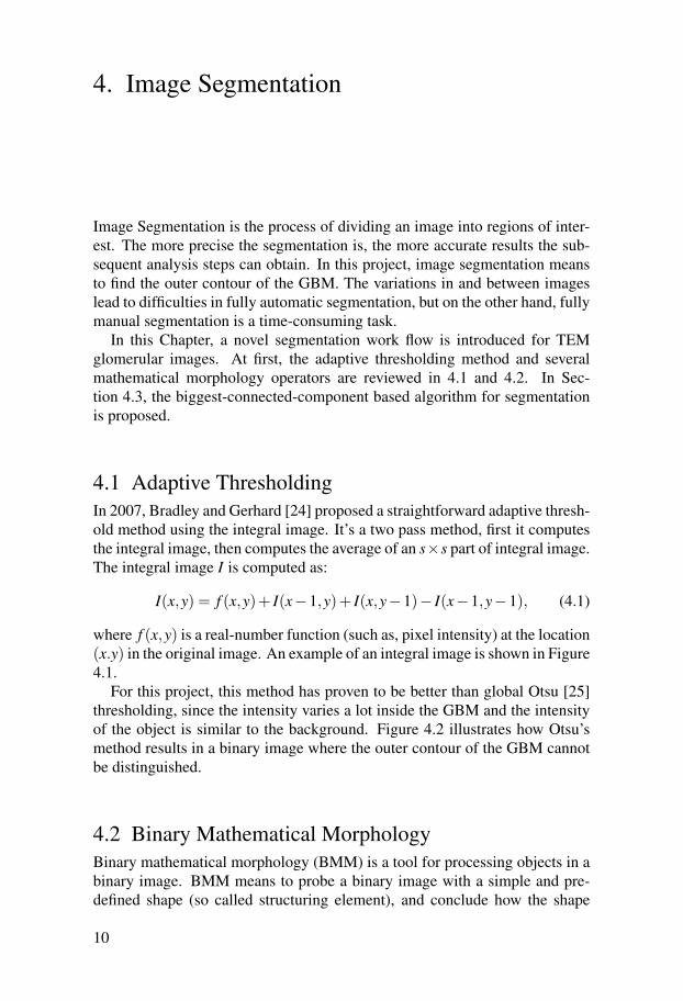
4. Image Segmentation

Image Segmentation is the process of dividing an image into regions of inter-est. The more precise the segmentation is, the more accurate results the sub-sequent analysis steps can obtain. In this project, image segmentation meansto find the outer contour of the GBM. The variations in and between imageslead to difficulties in fully automatic segmentation, but on the other hand, fullymanual segmentation is a time-consuming task.

In this Chapter, a novel segmentation work flow is introduced for TEMglomerular images. At first, the adaptive thresholding method and severalmathematical morphology operators are reviewed in 4.1 and 4.2. In Sec-tion 4.3, the biggest-connected-component based algorithm for segmentationis proposed.

4.1 Adaptive ThresholdingIn 2007, Bradley and Gerhard [24] proposed a straightforward adaptive thresh-old method using the integral image. It’s a two pass method, first it computesthe integral image, then computes the average of an s×s part of integral image.The integral image I is computed as:

I(x,y) = f (x,y)+ I(x−1,y)+ I(x,y−1)− I(x−1,y−1), (4.1)

where f (x,y) is a real-number function (such as, pixel intensity) at the location(x.y) in the original image. An example of an integral image is shown in Figure4.1.

For this project, this method has proven to be better than global Otsu [25]thresholding, since the intensity varies a lot inside the GBM and the intensityof the object is similar to the background. Figure 4.2 illustrates how Otsu’smethod results in a binary image where the outer contour of the GBM cannotbe distinguished.

4.2 Binary Mathematical MorphologyBinary mathematical morphology (BMM) is a tool for processing objects in abinary image. BMM means to probe a binary image with a simple and pre-defined shape (so called structuring element), and conclude how the shape

10

(a) (b)

Figure 4.1. An example of integral image. a) The original image. b) The computedintegral image based on a).

(a) (b) (c)

Figure 4.2. Comparing adaptive thresholding with the global thresholding usingOtsu’s method. a) Image after pre-processing. b) The result of adaptive threshold-ing. c) The result of Otsu’s global thresholding.

hits or misses the objects in the image. There are four basic BMM operators:erosion, dilation, opening and closing. Beside the four basic operators, theboundary can be obtained by subtracting a dilated image from the original im-age. In this project, only erosion (), dilation (⊕) and BMM edge extraction(∂ ) are used. These operators, which are applied to a binary image A using astructuring element B, are defined as:

Erosion : AB = x|Bx ⊆ A, (4.2)

Dilation : A⊕B = x|Bx∩X 6= 0, (4.3)Edge : ∂A = A (A⊕B), (4.4)

where x is the set of positions inside the structuring element B, Bx is the re-flection of Bx.

If the object is white and the background is black, then applying erosionproduces a darker image, as it removes small objects. Dilation produces an

11

opposite result with thickened objects. With a 3× 3 square structuring ele-ment, BMM edge extraction produces a one-pixel-wide curve, which can beused in the chain code algorithm [19] for length calculation. The results of thethree BMM operators are illustrated in Figure 4.3.

(a) (b)

(c) (d)

Figure 4.3. Results of BMM where the background is black and the object is white,using a 3×3 square structuring element. a) Original binary image. b) Eroded imageof a). c) Dilated image of a). e) Edge Image of a).

4.3 Segmentation AlgorithmIn manual measurement of the dataset, the glomerular which needs to be mea-sured, is always the biggest component in the image, and the outer contour ofthe GBM is also the longest curve. Based on these assumptions, a biggest-connected-component-based algorithm is proposed to specify the outer con-tour of the GBM.

12

After pre-processing, this algorithm first applies the adaptive thresholdingmethod described in Section 4.1 and removes small objects, which are lessthan 20× 20 pixels in size. After that, a binary erosion is used to fill thesmall gaps between two foot processes. At last, the binary boundary extractionoperator is applied to get single-pixel-wide lines. The longest connected linein the image is considered as the outer contour of the GBM. The work flow isshown in algorithm 1 (the membrane segmentation algorithm).

By default, the structuring element is a disk with a diameter of 7 pixels forthis dataset. This parameter affects the results of the segmentation. If it is toolarge or too small, the outer contour of the GBM cannot be correctly detected.The results for different sizes of the parameter are illustrated in Figure 4.4. Tomake the results clearly visible , all detected curves are shown as bold red linesin this report. A tip for choosing proper structuring element size is to reducethe size if the detected line goes inside the outer membrane and vice versa.

(a) (b) (c)

Figure 4.4. Edge information for different sizes of the structuring element. a) Theproper element size with a diameter of 5 pixels. b) A bigger element size with adiameter of 9 pixels. c) A smaller element size with a diameter of 3 pixels.

4.4 Manual SegmentationManual segmentation is supported by letting the user add anchor points on theouter contour of the GBM, then Cardinal splines are created based on theseanchor points.

Based on [26], a Cardinal spline is a sequence of individual curves joinedto form a large curve with a tension parameter. If the tension equals zero, itcorresponds to infinite physical tension, which means straight lines betweenpoints; if the tension equals one, it corresponds to no physical tension, whichallows the splines to take the path of least total bend; if the tension is largerthan one, the curve behaves like a compressed spring curve and will take alonger path. The effects of the tension parameter are shown in Figure 4.5.

13

Algorithm 1 Membrane Extraction AlgorithmInput: Original TEM image OriMapBinary Morphology structuring element size GapSizeOutput: The edge image corresponding to the outer membrane of the GBMEdgeMap1. Assign OriMap to EdgeMap// the pre-processing;2. Apply adaptive smoothing filter in EdgeMap.3. Apply a Gaussian sharpening filter in EdgeMap.// biggest-connected-component based algorithm5. Apply adaptive local thresholding method in EdgeMap.6. Remove small black objects that smaller than 20*20 in EdgeMap.7. Binary erosion using GapSize.8. Extract the biggest connected component in EdgeMap.9. Invert Colour of EdgeMap.10. Apply binary erosion using GapSize.11. Extract biggest connected component in EdgeMap.12. Invert Colour of EdgeMap.13. Apply binary edge extraction operator to edgeMapReturn: EdgeMap

With manual segmentation, the user adds anchor points on the contour, andthen cardinal splines are used to interpolate between points with a tensionequal to 1.

Figure 4.5. Cardinal splines with different tensions.

14

5. Membrane Length Calculation

After segmentation, a closed one-pixel-wide curve is obtained. Sometimesonly part of the curve is needed for measuring, so by assigning the start point,end point and the search direction, the length can be obtained.

In this chapter, the chain coding algorithm is described in Section 5.1 andcurve smoothing and length measurement are described in Section 5.2 andSection 5.3. Manual correction is shown in Section 5.4.

5.1 Chain CodeLength measurement of curves has been studied for a long time. Dating backto 1961, Freeman [27] segmented digital lines into n+1 grid points, then the nvector elements connected the grid points. The coding of the vector elementsis called the chain code . The interpretation of chain code numbers is triviallyexplained with Figure 5.1a. The circle in the Figure is the current point, andthe curve shown in Figure 5.1b has the chain code [1 0 7 5 4].

(a) (b)

Figure 5.1. The chain code. a) 8-connected chain code. b) An example of chain code.

Then later, based on the chain code, Vossepoel and Smeulders [19] derivedthe optimal values to measure the length of a curve, by using even, odd andcorner counts. The equation is:

Length = ∑even∗0.980+∑odd ∗1.406−∑corner ∗0.091, (5.1)

where corner counts means the number of times the chain code changes value.This method is very accurate, less than 1 % error is reported [19].

15

5.2 Curve SmoothingSometimes the edge information obtained from the segmentation algorithm isnot smooth enough, as illustrated in Figure 5.2a. There are some extremelyspiky parts and stair-like parts in the curve. Since the membrane is consideredto be a smooth curve, these are unwanted features and need to be removedbefore measuring the length.

To smooth the curve, two characteristics are used: the distance between 2points and the angle differences between three points along the curve withinsome range. In each iteration, the algorithm keeps points that meet the condi-tions below:

∀p1 = (x1,y1), p2 = (x2,y2), p3 = (x3,y3) in the curve location list

angle = arctany2− y1

x2− x1− arctan

y2− y3

x2− x3< AngleTolerance, (5.2)

distance =√(x1− x2)2 +(y1− y2)2 < DistanceTolerance, (5.3)

where p1, p2, p3 are points on the outer contour of GBM. p2 is step away fromp1 and p3 is also step away from p2. The first criteria removes ”Λ” like partsand the second removes ”Ω” like parts.

Figure 5.2b shows the result of the curve smoothing algorithm. The systemalso provides the opportunity to manually correct the results, and the result ofthe manual correction is shown in Figure 5.2c.

(a) (b) (c)

Figure 5.2. a) A detected curve from segmentation algorithm. b) Smooth curve. c)Manually corrected curve of b).

By default the AngleTolerance and DistanceTolerance are set to 15 (ap-proximately 0.26 radians) and 10 pixels. This algorithm is presented as Algo-rithm 2 (the curve smoothing algorithm).

16

Algorithm 2 Curve Smoothing AlgorithmInput:A list of pixels listAn integer for calculation stepDistance Tolerance disTolAngle Tolerance angTolOutput:A list of pixels for a smooth curve newList

counts is the first element in the liste is the element that step away from sw is the element that count away from sAdd s into newListwhile count < the number of pixels in list do

if the angle difference between line s to w and line w to e > angTolthen

Check every point backward from e to w, find the farthest f ar one whichthe angle difference > angTol.

w← f arif w is not in list list thenAdd w into newListCheck pixels after w in list list, find the first position j with angle dif-

ference < angTol & the distance of jth point to line wth point to sth point <disTol

Add jth element of list into list newListcount← j+ steps← we← jth element of list

Return: newList

17

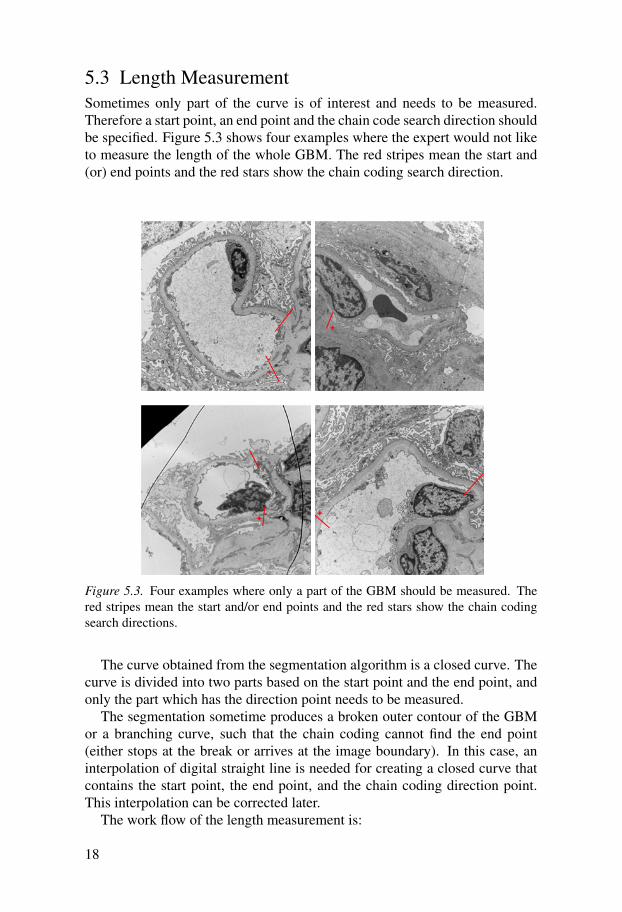
5.3 Length MeasurementSometimes only part of the curve is of interest and needs to be measured.Therefore a start point, an end point and the chain code search direction shouldbe specified. Figure 5.3 shows four examples where the expert would not liketo measure the length of the whole GBM. The red stripes mean the start and(or) end points and the red stars show the chain coding search direction.

Figure 5.3. Four examples where only a part of the GBM should be measured. Thered stripes mean the start and/or end points and the red stars show the chain codingsearch directions.

The curve obtained from the segmentation algorithm is a closed curve. Thecurve is divided into two parts based on the start point and the end point, andonly the part which has the direction point needs to be measured.

The segmentation sometime produces a broken outer contour of the GBMor a branching curve, such that the chain coding cannot find the end point(either stops at the break or arrives at the image boundary). In this case, aninterpolation of digital straight line is needed for creating a closed curve thatcontains the start point, the end point, and the chain coding direction point.This interpolation can be corrected later.

The work flow of the length measurement is:

18

• Run chain coding to find the curve part, which contains the start point,the end point and the direction point. If the end point cannot be arrivedat, interpolate a straight line between the last point that can be obtainedand the end point.

• Run curve smoothing algorithm to remove unwanted structures andget a smooth curve.

• Run chain coding again to count the odd, even and corner chain codes,and calculate the length.

5.4 Manual Correction in Length MeasurementIf the segmentation and/or length measurement are not good enough, a manualcorrection possibility is provided just after automatic length measurement andbefore the ”slits” counting.

By marking a number of anchor points on the desired outer contour of theGBM, the algorithm finds the nearest point of the first click and the last click,then it removes all anchor points located between these two points. New an-chor points are then added in this space. An example of this procedure isshown in Figure 5.4.

Figure 5.4. The manual correction procedure. The solid line is the detected line andthe red dots are anchor points from length measurement. The red stars are manuallyadded anchor points which forces the Cardinal splines to follow the dashed lines, andthe dashed lines refer to the outer contour of the GBM.

The original anchor points either come from manual segmentation or in-terval values in the locations of curve pixels which were obtained from thework flow in Section 5.3.Then the Cardinal splines (Section 4.4) are used forre-interpolating the anchor points.

The work flow for manual correction in Length measurement, is as follows:• Get anchor points list: The program either gets anchor points directly

from manual segmentation (if it is used) or gets interval values of the

19

curve pixels’ locations from the automatic length measurement (Section5.3).

• Compute new anchor points: After the user marks new anchor pointson the outer contour of the GBM, the algorithm locates the first and lastclick in the anchor points list, then removes all anchor points betweenthe two, and adds the newly clicked anchor points.

• Interpolate new anchor points list: The Cardinal splines are used tointerpolate all the anchor points, and then runs chain coding again toupdate both location information and length information.

20

6. Slits Counting

Counting ”slits” is the last step of the measurement, and a local method is de-veloped for this purpose. The ”slits” counting algorithm creates a binary im-age using Otsu’s method (Section 6.1) and a gradient image (Section 6.2). To-gether with the outer contour of the GBM, the ”slits” are detected and counted.

6.1 Binary Images in Slits CountingOtsu’s thresholding method is a well-known global thresholding method whichis based on the grayscale histogram. The optimal threshold k? is the maximumof δ 2

B(k),which is computed as:

δ2B(k) =

[µT ω(k)−µ(k)]2

ω(k)[1−ω(k)], (6.1)

where

ω(k) =k

∑i=1

pi, (6.2)

µ(k) =k

∑i=1

ipi, (6.3)

µT = µL =L

∑i=1

ipi. (6.4)

Here L is the upper bound of the gray levels for the image, pi is the probabilitydistribution, such that pi = ni/N, and N is the number of pixels in the image.ni is the number of pixels of the gray level i.

In this project, Bradley’s [24] thresholding (adaptive thresholding) methodis only used for segmenting the outer boundary of the GBM. Compared toOtsu’s method, the Bradley’s [24] thresholding method doesn’t preserve thefoot processes. A comparison is shown in Figure 6.1.

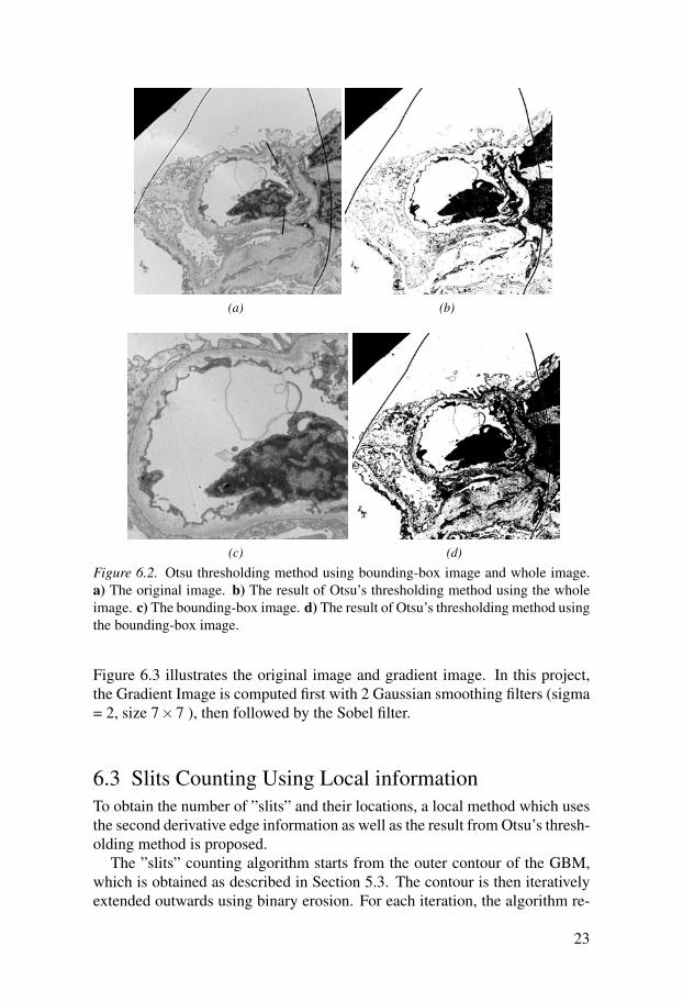
When the whole image is the input to Otsu’s thresholding method, thereis a special case when the shape of foot process is not kept, shown in Figure6.2b. In this image, there is a big black area which influences the result a lot.By using the bounding-box image to compute the Otsu’s thresholding value, abetter result can be obtained. The result of Otsu’s thresholding method usingbounding-box image is shown in Figure 6.2d, and the bounding-box imageis illustrated in Figure 6.2c, where the measurement started and ended at theblack stripe in Figure 6.2a

21

(a) (b) (c)

Figure 6.1. Result images for adaptive and Otsu’s global Thresholding. a) The originalimage. b) The result of Otsu’s global thresholding method. c) The result of adaptivethresholding method.

6.2 The Gradient ImageIn a gray scale image, an image gradient is a directional change of intensity.Mathematically in a 2-D image, it is a two-variable function, which is definedas:

∇ f =δ fδx

X +δ fδy

Y, (6.5)

where f is a 2-D image,δ fδx

X is the gradient in x-axis andδ fδy

Y is the gradient

in y-axis. The gradient direction is calculated as:

θ = atan2(δ fδy

,δ fδx

). (6.6)

Gradient images can be obtained from the original image convolved with afilter. One of the simplest filters is the Sobel filter. Sobel filter uses two 3×3convolution kernels:

Gx =

1 0 +12 0 +21 0 +1

∗ I, (6.7)

Gy =

1 2 10 0 0+1 +2 +1

∗ I, (6.8)

where I is the source image, Gx and Gy represent the horizontal and the verticalderivative approximations. For each point, the resulting gradient magnitudeapproximation is:

G =√

G2x +G2

y . (6.9)

22

(a) (b)

(c) (d)

Figure 6.2. Otsu thresholding method using bounding-box image and whole image.a) The original image. b) The result of Otsu’s thresholding method using the wholeimage. c) The bounding-box image. d) The result of Otsu’s thresholding method usingthe bounding-box image.

Figure 6.3 illustrates the original image and gradient image. In this project,the Gradient Image is computed first with 2 Gaussian smoothing filters (sigma= 2, size 7×7 ), then followed by the Sobel filter.

6.3 Slits Counting Using Local informationTo obtain the number of ”slits” and their locations, a local method which usesthe second derivative edge information as well as the result from Otsu’s thresh-olding method is proposed.

The ”slits” counting algorithm starts from the outer contour of the GBM,which is obtained as described in Section 5.3. The contour is then iterativelyextended outwards using binary erosion. For each iteration, the algorithm re-

23

(a) (b)

Figure 6.3. a) The original image. b) The gradient image.

computes the curve location list using chain coding, which is explained inSection 5.1. Then, each point in the list compares the colour to the previouspoint in the same list, the change of colour (white to black, or black to white)refers to a ”slit” candidate.

To be a true ”slit”, two criteria should be met:• Distance Criterion: ∀ point pi = (x1,y1) and pi+1 = (x2,y2) where pi

is the ith element in curve location list L, distance between pi and pi+1should be less than the distance tolerance.

distance =√(x1− x2)2 +(y1− y2)2 < DistanceTolerance. (6.10)

• Percentage Criterion: ∀ point pi = (x1,y1) in the curve location list L,computes the local s× s sub-image B(x1− s

2 ,y1− s2 ,s,s) of the gradi-

ent image I. Then count the number of pixels, which have the intensitylarger than a gradT hreshold. The ratio of the number to the total integralimage pixel number(s×s) should be larger than a percentageTolerance.

By default s = 9, gradT hreshold = 60, DistanceTolerance = 11 andpercentageTolerance = 0.6. Tracing the number of ”slits” in each iteration,the sequence produces either a double-peaked curve or a logarithmic-shapedcurve within a certain range of distance from the outer contour of the GBM.The two kinds of curves are shown in Figure 6.4a, and the actual number of”slits” marked manually by the expert is shown in the dashed box. It is clearthat the number of ”slits” corresponds to the automatic count around the peaksor in the middle of the range when there is no peak. The algorithm for tracingthe number of ”slits” is shown in Algorithm 3. The positions can be manuallycorrected by the user. An example of potential ”slits” counts are shown inFigure 6.4b and 6.4c, the manual correction based on the second potential”slits” counts is shown as Figure 6.4d.

24

Algorithm 3 ”Slits” counting AlgorithmInput:A list of pixels list of the membraneAn integer of maximum erosion time maxDistance Tolerance disTolThe result from Otsu’s method binaryMapThe Edge information gradMapEdge Percentage Tolerance gradTolThe Local Consideration Size localAreaThe Threshold value of gradT hresholdOutput:A list of ”slits” locations newList

count = 0A new list to store the result newListwhile count < the number of elements in list do

if the color of countth points differs from the (count + 1)th inbinaryMap

add the (count +1)th point into newListcount+= 1

count = 0while count < the number of elements in newList do

if the distance between the countth point and the (count +1)th point isless than disTol

remove the countth element form newList

count = 0pixels = 0while count < the number of elements in newList do

Copy the localArea× localArea sub-image from gradMap and its cen-tral point is the countth point in newList

forall Pixels in the sub-imageif the grey value is larger than gradT hresholdpixels+= 1if percentage = pixels/localArea/localArea < gradTolremove the countth element of newList

Return: newList

25

(a) (b)

(c) (d)

Figure 6.4. a) The trends for the number of ”slits” counts. The candidate ”slits” countfor the logarithmic-shaped curve is around the middle in the middle of the range. Forthe double-peaked curve, the candidate ”slits” counts correspond to the peaks. b) Thefirst potential ”slits” counts. c) The second potential ”slits” counts. d) The manualcorrection of ”slits” based on c).

26

7. Results and Evaluation

The data set tested consists of samples from five patients, and for each pa-tient 6 images are acquired. All the images are TEM images of kidney tissuesamples with glomerulars. Every image has one glomerular (a whole one, orpart of one) that covers a large area, and some images also contain lsmallerglomerular parts located on the boundary. The shape of glomerulars varies alot, from circle to star, from pentagon to shell, etc.

All tests are performed in Window 7 64-bit, Intel(R) Core(TM) i7 2.67 GHzwith debug mode under Microsoft Visual Studio 2010. The TEM images are2048 × 2048 pixels in size, and the sale is 0.008 µm/ pixels. All images are8-bit grayscale images stored using TIFF file format. The scale information isobtained from the TIFF header.

7.1 Segmentation EvaluationWith a suitable structuring element size, the segmentation algorithm suffi-ciently well segments more than 95% of the images (the segmentation failedonly on one out of 30 images). Figure 7.1 shows the segmentation results ofthree images from three patients.

The first image is well segmented, the segmentation of the second one andthe third one are not perfect, due to the fuzzy dark area around the outer con-tour of the GBM. A disk-shaped structuring element with the diameter equalto 7 pixels is used for first two cases and the diameter is 5 pixels for the third.

Figure 7.2a shows how the structuring element size influences the process-ing time. The bigger the structuring element size is, the longer processing timethe segmentation takes. As illustrates in Figure 7.2b, the most used structuringelement size was 7 (the default value), and it is applicable to most cases. Thebad segmentation can be smoothed automatically and (or) corrected manuallylater in the length measurement stage.

7.2 Length MeasurementA closed single-pixel curve is derived from the segmentation. Since the lengthmeasurement is based on chain coding, it will fail (but give a value whichcan be corrected manually) when the segmentation produces a disconnected

27

(a) (b) (c)

Figure 7.1. Some segmentation result images. a) Well segmented image using a diskstructuring element with the diameter equal to 7 pixels. b) Segmentation image withaverage difficulty using the same structuring element as in a). c) A difficult imageusing a disk structuring element with the diameter equal to 5 pixels.

outer contour of the GBM or a branching curve. With manual correction, thisproblem can be fixed.

By specifying the start point, the curve direction and the end point, the al-gorithm finds the part of interest and removes unwanted regions. Figure 7.3illustrates the length measurement results after curve smoothing and manualcorrection. The images presented are the same as those presented in the seg-mentation evaluation. The length measurement results are 23.5 µm, 43.8 µmand 33 µm for the proposed method with manual correction. The correspond-ing expert manual measurements are 22.2 µm, 41.2 µm and 32.1 µm.

Figure 7.4a shows a comparison of the length measurements from the pro-posed method and the expert. By Comparing all lengths obtained from theproposed method with the lengths from the expert’s measurements, as Figure7.4a shows, it is clear that the length measurements of the proposed methodslightly over estimates the expert’s measurements. The overestimation seemsto be approximately linearly related to the expert’s measurements, and the lin-ear regression coefficient matrix is A = [1.051 1.506].

The percent error of the lengths obtained from the proposed algorithm rela-tive to the expert’s measure is plotted in Figure 7.4b. The average is 10 % andthe standard deviation is 0.06. The percent error δ is defined as:

δ =|v− vapprox||v|

×100%, (7.1)

where v is the length measurement for the expert and the vapprox is the lengthmeasurement from the proposed method.

28

(a) (b)

Figure 7.2. The structuring element size and run time. a) The segmentation run timefor each of the 30 images. b) The structuring element size distribution.

7.3 ”Slits” CountingAfter the length measurement phase, the ”slits” are counted. As described inChapter 6, the extended-outwards algorithm calculates the sequence of ”slits”,and provides one or two candidate ”slits” counts.

For all 30 images, the method takes an average 38.84 seconds to find thecandidate ”slits” locations. At most it takes 40.95 seconds. Figure 7.5 showsthe run times for the 30 images.

Sub-figures in Figure 7.6 show examples of the two candidate ”slits” counts,which are marked as red dots in the figures for the same images used in pre-vious sections. Table 7.1 illustrates ”slits” number from the expert. ”Slits”numbers from the two candidate ”slits” counts from the proposed method. Ascan be seen from the Table 7.1, at least one of the counts is close to the expert’smeasurement.

Table 7.1. The number of ”slits” for three images used in the previous sections.

Cases ”slits” number ”slits” number, ”slits” number,from expert counts 1 counts 2

Case 1 43 46 47Case 2 12 6 12Case 3 38 34 38

Figure 7.7a illustrates the relationship of ”slits” counts between the pro-posed method and the expert measurements. By choosing the better one fromthe two candidate counts, the results turn out to be as Figure 7.7b. The chosen

29

(a) (b) (c)

(d) (e) (f)

Figure 7.3. Some length measurement result images. a-c) The outer contours ofthe GBMs from the automatic length measurement. d-f) Corresponding manuallycorrected results of a-c).

counts are much closer to the diagonal, which means a better result. Only thenumber of ”slits” counts are compared to the expert’s measurements, locationsare not.

As mentioned in Chapter 1, for a sample to be classified as FPE the mea-surement slits/µm GBM should be less than 1.0 . To find the FPE patients, theslits/µm GBM is measured. The measurement results for 5 patients (each ofthem has 6 images) are listed in table 7.2, Patient 4 is distinguished from theothers since this patient has a small average slits/µm GBM. These results arealso plotted in Figure 7.8 where the error bars are used to present the standarddeviations.

30

(a) (b)

Figure 7.4. a) The length comparison. b) The percent errors of the length measure-ments.

Figure 7.5. The run times for counting ”slits”.

Table 7.2. Measurement Comparison from Expert and My Method for five patients.

Average of Average of”slits” per µ m ”slits” per µ m Stand deviation Stand deviation

Patient from expert from my method from expert from my methodPatient 1 1.8831 1.5108 0.3169 0.2555Patient 2 1.3093 1.079 0.3963 0.4225Patient 3 1.0905 1.1198 0.1722 0.1958Patient 4 0.4353 0.4211 0.0925 0.1795Patient 5 1.2026 1.1368 0.2673 0.2334

31

Figure 7.6. ”Slits” measurement results for the same images used in the previoussections. The left column: One ”slits” count for the three images. The right column:Another ”slits” count.32

(a) (b)

Figure 7.7. Results of ”slits” counts comparing to the expert measurements for all 30images. a) The two candidate ”slits” counts, the stars and circles refer to two counts.b) The chosen ”slits” counts.

Figure 7.8. The standard deviation and the mean values for the five patients. To makethe error bars clearer, the data from the expert is slightly shifted to the right.

33

8. Programming Framework

In the previous chapters I described the methods, work flows and the results.In this Chapter, two frameworks used for implementing GUI and methods aredescribed.

8.1 MS .Net FrameworkMS .Net Framework [28] is a comprehensive and consistent programmingmodel, it provides services for building, deploying and running desktop, weband phone applications and web services.

A little like Java, MS .Net framework never lets the user directly connect tothe hardware level in a managed application. All works are handled in a layerupon the operating system/ hardware level, as shown in Figure 8.1. This layer,called the common language runtime (CLR), together with an extensive classlibrary constitute the main .Net Framework.

CLR provides core services such as memory management, thread manage-ment, while also enforcing strict type safety and other forms of code accuracy.The extensive library is an object-oriented collection of reusable types for de-velopment ranging from traditional command line or GUI to Web forms orweb services.

Figure 8.1. .Net Framework in Content.

The .Net Framework can be hosted by both managed and unmanaged com-ponents. Interoperability between managed and unmanaged code enables de-velopers to continue to use necessary component object model (COM) com-ponents and dynamic-link libraries (DLLs). This is commonly used for as-sembling and installing third party libraries and for large solutions which haveseveral small projects.

34

Using the .Net Framework, many applications can be built, such as Win-dows GUI applications, console application, web services, etc. The latest sta-ble version is .Net Framework 4.0 for both 32-Bit and 64-Bit operating sys-tems. For efficiency reasons and third party libraries, the software developedfor this thesis project contains both managed and unmanaged components.

8.2 AForge.NetAForge.NET is an open source C# framework designed for developers andresearchers, it provides functions for image processing, neural networks, fuzzylogic, robotics, etc. For this thesis project, libraries for image processing andmathematics were used.

The framework [23] has a set of namespaces, the largest one is AForge.Imaging,it contains image processing routines, such as colour spaces, mathematicalmorphology operations, edge detection algorithms, convolutions, image for-mats, etc. Another namespace used is AForge.Math, it contains different al-gorithms, which are used internally by the framework.

The developing language is C# .Net so the framework can be easily ac-cessed by the .Net framework, and both 32-Bit and 64-Bit versions are avail-able now. Figure 8.2 shows some of the methods used in the project and theclasses relationship under the AForge.Imaging namespace. As the biggest li-brary of AForge, it provides more than 150 classes for image processing intotal.

Figure 8.2. The Class Relationship of AForge.Imaging.

35

9. Software design and Implementation

Based on the two frameworks described in chapter 8, my tool was built up asa Windows form application, which runs under Windows.

9.1 Software ArchitectureThe software pattern used for my project is Model-View-Controller (MVC),as shown in Figure 9.1, it divides an application into three components: theModel, the View and the Controller. The Model is used to describe data struc-tures (domain objects), the View together with the Controller interacts withthe user, the View presents the results and the Controller translates the userinput to what can be understood by the Model.

In this project, the Model is divided into two parts: the Dataset and the Pro-cessing. The Dataset provides data structures for storing and transmitting dataamong different algorithms in the Processing part. The Processing contains allalgorithms and work flows described in Chapter 3 to Chapter 6.

Figure 9.1. The software pattern MVC.

In MS .Net framework, all projects should belong to a solution. In thisthesis, 5 different projects are created with different functionalities under the”Thesis Solution”, as shown in Figure 9.2. The project ”Thesis” helps controlthe windows forms events and software states. The ”Picturebox” providesfunctions for presenting images, such as zooming, scrolling, and marking. The”Data” handles all data structures that are used for exchanging informationamong algorithms in ”Processing” and user input from ”Thesis”. So project”Thesis” works as Controller and the ”Picturebox” works as the View andproject ”Data” and ”Processing” work together as the Model in MVC.

36

Figure 9.2. Thesis Solution Architecture.

Figure 9.3. The graphic user Interface.

9.2 GUI and ImplementationThe GUI has been divided into two parts (excluding the menu bar at the top):the work flow area, and the work space, as shown in Figure 9.3.

The work flow area contains several small parts: the segmentation, thelength measurement, the manual correction of contour, ”slits” counting, andthe measurement results.

After the image is loaded, the pre-processing together with the segmenta-tion can be done by pressing the button with the letter ”A”. The user can alsomanually segment the image by adding anchor points on the outer contour ofthe GBM in the work space (the biggest area with the image, where the imagecan be zoomed) after pressing the button with the letter ”M”. The folder buttonapplies the segmentation to all images in same folder.

There are two options for the length measurement, either the shape of theGBM is a circle where only the start point is needed, or the start point, the

37

Figure 9.4. Content of an example result file, stored on disk as a .txt text file.

end point and chain coding direction point are needed. These two optionscorrespond to the buttons in the second part of the work flow area.

The ”slits” counting can be done after manual correction of the outer con-tours of the GBM (this step can be skipped if the GBM is automatically wellsegmented), and specifies the inner part of object (the black button). The threebuttons in the fourth part correspond to the two ”slits” counts and manualmarking. Using the first two buttons, the user can observe the two ”slits”counts and manually correct them. The last button corresponds to the manual”slits” measurement.

The result is presented in the measurement results part (the left bottom partof the work flow area). The result can also be stored in a txt file in the samefolder where the images (for the same patient) are located. As shown in figure9.4, the data is separated with semicolon, and the components saved are filename, length of GBM in µm, the number of ”slits” and the value of ”slits” perµm. The last two lines show the averages and standard deviations.

38

10. Summary and Conclusion

10.1 SummaryThe developed tool provides a GUI and a set of functions for FPE measure-ments in TEM images of kidney tissue samples. The procedure consists ofthree main stages: segmentation, length measurement and ”slits” counting.

In the segmentation stage, the basic assumption was that the glomerularsneeded to be measured were always the biggest connected components in theTEM images. So the segmentation method extracted the biggest connectedcomponent after pre-processing, adaptive thresholding and binary mathemati-cal morphology. As expected, the adaptive thresholding method gave a betterresult in distinguishing the GBM from foot processes than the global Otsumethod. However, weak edge information might be lost.

In the length measurement stage, a chain-code based algorithm has beenproposed to measure the length and smooth the curve. With a specified startpoint, an end point and a search direction, the algorithm removed some un-wanted parts from the segmented curves and fixed the curves at the two endsby using angle differences and the distances between line points. It required aclosed single-pixel curve without branches from the segmentation algorithm.However, the segmentation algorithm would produce a branching and/or dis-connected curve, and the length measurement algorithm could give a reallypoor result as well, if the outer contour of the GBM was too weak to detect,and the size of structuring element could not be found. In this case, a man-ual correction or a manual segmentation could be used. The automaticallymeasured lengths were a bit over estimated compared to the manual expertmeasurements.

The ”slits” measurement came in the third stage. For each iteration, ”slits”counts were computed along the contour by using local information in a gra-dient image and Otsu’s thresholding image, and then the contour extendedoutwards. In some specified ranges, the ”slits” count sequence followed atwo-peak curve or a logarithmic curve. The proper ”slits” locations were areat the one peak (the first or the second peak) or at the centre of the specifiedrange. This produced two ”slits” count candidates, and the user could chooseone ”slits” count and correct it, or even manually counted ”slit” locations fora very difficult image. Furthermore, according to our evaluation, the repeateduse of BMM operators, which was used to extend the contour, consumed halfof the execution time, as it went through the whole image pixel by pixel witha small kernel for each iteration.

39

The tool provides automatic measurement with chances for correcting, aswell as manual measurement based on the .NET framework and AForge Frame-work 2.2.4. After the length measurement stage, there is a chance to correctthe detected boundary of the GBM. Then after the ”slits” measurement, theuser can always choose one ”slits” group and correct them manually. Bothsegmentation and ”slits” counting can be done manually. A GUI for all func-tionalities, along with image presentation handling, is provided by this tool.

To evaluate the algorithms and work flow, data from five patients (eachof them had six images) were used. Both the computational time and theaccuracy were evaluated. With a proper structuring element size, the tool canprovide results within minutes, and the FPE patient has been distinguishedsuccessfully.

10.2 Conclusion and Future WorkDuring the master thesis, a semi-automatic analysis tool for FPE detection ofkidney samples in TEM images has been successfully designed and imple-mented, the purposes set in Section 1.2 were fulfilled. This tool works underWindows operating system. It combines numerous image analysis methods,with a GUI to present the results and to help the user access all the functionseasily. An automatic analysis procedure, a manual correction and a manualmeasurement are all included in this tool.

However, a limitation of the current length measurement is that only aclosed one-pixel-wide curve without branches can be accepted by the lengthmeasurement algorithm. It might be interesting to try to combine with othersegmentation methods mentioned in Chapter 2 to get the whole GBM, or an-other smarter way is to choose the structuring element for BMM dynamically.Otherwise a better length measurement method, which handles the branchingcurve and disconnected curve, is needed.

Another limitation is that the user needs to select one ”slits” candidate (ifthere are two candidate sets) manually. It might be helpful to select the bettercandidate set by using the curvature of foot processes and (or) track the wholefoot processing.

To improve the efficiency of the system, reducing the run time of BMMoperators is important. In the other hand, the system is developed with only30 images, so it would benefit of a larger test set or some more evaluationswith new TEM images.

40

References

[1] M. Carroll, J. Temte et al., “Proteinuria in adults: a diagnostic approach,”American family physician, vol. 62, no. 6, p. 1333, 2000.

[2] F. Dunér, Ultrastructural studies of the blood-urine barrier in proteinuric states.Karolinska institutet, 2010. [Online]. Available:http://books.google.se/books?id=CAc6cgAACAAJ

[3] S. Choi, K. Suh, D. Choi, and B. Lim, “Morphometric analysis of podocyte footprocess effacement in iga nephropathy and its association with proteinuria,”Ultrastructural Pathology, vol. 34, no. 4, pp. 195–198, 2010.

[4] S. Shankland, “The podocyte’s response to injury: role in proteinuria andglomerulosclerosis,” Kidney international, vol. 69, no. 12, pp. 2131–2147, 2006.

[5] K. Hultenby, “Personal communication,” May 2012.[6] I. Kamenetsky, R. Rangayyan, and H. Benediktsson, “Segmentation and

analysis of the glomerular basement membrane using the split and mergemethod,” in Engineering in Medicine and Biology Society, 2008, pp.3064–3067.

[7] M. Frumar, Z. Cernosek, J. Holubova, and E. Cernoskova, HomogeneityThreshold in Sulphur Rich Ge-S Glasses. Defense Technical InformationCenter, 2001.

[8] R. Rangayyan, I. Kamenetsky, and H. Benediktsson, “Segmentation andanalysis of the glomerular basement membrane using active contour models,” inIET International Conference on Advances in Medical, Signal and InformationProcessing (MEDSIP), 2008, pp. 1–4.

[9] C. Xu and J. Prince, “Snakes, shapes, and gradient vector flow,” IEEETransactions on Image Processing, vol. 7, no. 3, pp. 359–369, 1998.

[10] J. Canny, “A computational approach to edge detection,” IEEE Transactions onPattern Analysis and Machine Intelligence, no. 6, pp. 679–698, 1986.

[11] K. Engel, M. Hadwiger, J. Kniss, C. Rezk-Salama, and D. Weiskopf, Real-timevolume graphics. Eurographics Association, pp. 112–114.

[12] T. Lindeberg, “Edge detection and ridge detection with automatic scaleselection,” in IEEE Computer Society Conference on Computer Vision andPattern Recognition, 1996, pp. 465–470.

[13] C. Steger, “An unbiased detector of curvilinear structures,” IEEE Transactionson Pattern Analysis and Machine Intelligence, vol. 20, no. 2, pp. 113–125, 1998.

[14] K. Raghupathy and T. Parks, “Improved curve tracing in images,” in IEEEInternational Conference on Acoustics, Speech, and Signal Processing, 2004(ICASSP’04), vol. 3, 2004, pp. iii–581.

[15] M. Sargin, A.Altinok, and K. B.S.Manjunath, “Tracing curvilinear structures inlive cell images,” IEEE International Conference on Image Processing (ICIP ),2007.

41

[16] W. Liao, A. Khuu, M. Bergsneider, L. Vese, S. Huang, and S. Osher, “Fromlandmark matching to shape and open curve matching: a level set approach,”UCLA CAM Report, vol. 2, no. 59, 2002.

[17] N. Paragios, M. Rousson, and V. Ramesh, “Matching distance functions: Ashape-to-area variational approach for global-to-local registration,” EuropeanConference on Computer Vision (ECCV), pp. 813–815, 2002.

[18] B. Lam and H. Yan, “A curve tracing algorithm using level set based affinetransform,” Pattern recognition letters, vol. 28, no. 2, pp. 181–196, 2007.

[19] A. Vossepoel and A. Smeulders, “Vector code probability and metrication errorin the representation of straight lines of finite length,” Computer Graphics andImage Processing, vol. 20, no. 4, pp. 347–364, 1982.

[20] T. Svoboda, J. Kybic, and V. Hlavac, Image Processing, Analysis & andMachine Vision-A MATLAB Companion. Thomson Learning, 2007.

[21] L. Matalas, R. Benjamin, and R. Kitney, “An edge detection technique using thefacet model and parameterized relaxation labeling,” IEEE Transactions onPattern Analysis and Machine Intelligence, vol. 19, no. 4, pp. 328–341, 1997.

[22] R. Haddad and A. Akansu, “A class of fast gaussian binomial filters for speechand image processing,” IEEE Transactions on Signal Processing, vol. 39, no. 3,pp. 723–727, 1991.

[23] AForge, “Aforge.net framework documentation version 2.2.4,”http://www.aforgenet.com/framework/docs/, AForge .NET Framework Group,Febrary 2012.

[24] D. Bradley and G. Roth, “Adaptive thresholding using the integral image,”Journal of Graphics, GPU, & Game Tools, vol. 12, no. 2, pp. 13–21, 2007.

[25] N. Otsu, “A threshold selection method from gray-level histograms,”Automatica, vol. 11, pp. 285–296, 1975.

[26] MSDN, “Cardinal splines,”http://msdn.microsoft.com/en-us/library/ms536358(v=vs.85).aspx, MSDNGroup, May 2012.

[27] H. Freeman, “On the encoding of arbitrary geometric configurations,” IRETransactions on Electronic Computers, no. 2, pp. 260–268, 1961.

[28] MSDN, “.net framework 4,”http://msdn.microsoft.com/enus/library/w0x726c2.aspx, MSDN Group, May2012.

42