imperial college london excitation method for thermosonic ... · imperial college london excitation...
TRANSCRIPT

IMPERIAL COLLEGE LONDON
EXCITATION METHOD FOR THERMOSONIC
NON-DESTRUCTIVE TESTING
by
Bu Byoung Kang
A Thesis submitted to the Imperial College for the degree of
Doctor of Philosophy
Supervised by Prof. Peter Cawley
Nondestructive Testing Laboratory
Department of Mechanical Engineering
Imperial College London
London SW7 2AZ
July 2008

Abstract
Thermosonics is a non-destructive testing method in which cracks in an object are
made visible through the local generation of heat caused by friction and/or stress
concentration. The heat is generated through the dissipation of mechanical energy
at the crack interfaces by vibration. The temperature rise around the area close to
the crack is measured by a high-sensitivity infrared imaging camera whose field of
view covers a large area. The method therefore covers a large area from a single
excitation position so it can provide a rapid and convenient inspection technique for
structures with complex geometry and small and closed cracks. An ultrasonic horn,
originally designed for welding, has generally been used for thermosonic testing.
However, it is difficult to obtain reproducible and controllable excitation with the
existing horn system because of non-linearity in the coupling; surface damage can
also be produced by chattering caused by loss of contact between the tip of the
horn and the structure. Therefore, the general aim of the study was to develop a
reliable and convenient excitation method that should excite sufficient vibration for
the detection of the defects of interest at all relevant positions in the structure and
must also avoid surface damage.
In this thesis, a numerical and experimental study for the development of the ex-
citation method for reliable thermosonic testing is presented. Successful excitation
methods for the detection of delaminations in composites and cracks in metal struc-
tures are described. A simple, small wax-coupled PZT exciter is introduced as a con-
venient, reliable thermosonic test system in applications where relatively low strain
levels are required for damage detection such as composite plates. A reproducible
vibration exciter may be sufficient for thermosonic testing in some metal structures
2
such as a thin plates. However, higher strain levels are often required in metal
structures, though the required strain level is dependent on the crack size. This
level of strain is not easily achieved within the reproducible vibration range because
of non-linearity in the contact between the exciter and the structure. Therefore,
studies are conducted with an acoustic horn with high power capability to investi-
gate the characteristics of the vibration produced in a real structure with complex
geometry and to develop a excitation method for achieving reliable excitation in
the non-linear vibration range for thermosonic testing. An excitation method for a
complicated metallic structure such as a turbine blade is also investigated and the
influence of the clamping method and the excitation signal that is input to the horn
on the vibration characteristics generated in the testpiece is presented. As a result,
a fast narrow band sweep test with a general purpose amplifier and stud coupling is
proposed as an excitation method for thermosonic testing. This method can be ap-
plied to different types of turbine blades and also to other components. One typical
characteristic of a thermosonic test using non-linear vibration is the lack of repeata-
bility in the amplitude and the frequency characteristic of the vibration. Therefore,
vibration monitoring is necessary for reliable thermosonic testing and a Heating In-
dex(HI) has been proposed as a criterion indicating whether sufficient vibration is
achieved in a tested structure or not. The HI is calculated from different vibration
records measured by different sensors and these results are compared in this thesis.
A microphone can provide a cheaper and more convenient non-contacting vibration
monitoring device than a laser or strain gauge and the heating index calculated by
a microphone signal shows similar characteristics to that calculated from the other
sensors.
3

Acknowledgements
I would like to express my gratitude to my supervisor Prof. Peter Cawley for his
invaluable guidance and encouragement during this work. I would also like to thank
all the colleagues of the NDT Laboratory. They have provided sound technical
support, inspirational discussions and great encouragement throughout the project.
I have thoroughly enjoyed my time working with you all.
In particular, I want to acknowledge the co-operation with Dr. Morbidini Marco.
Much of our work has been the result of our synergies.
Furthermore, I have to acknowledge the Engineering and Physical Sciences Research
Council (EPSRC), which has primarily funded this work, and the sponsorship of the
following industrial partners: AIRBUS, Rolls-Royce, BNFL and dstl.
Last (but not less important), I would like to heartily thank all those people who have
sincerely cared for me during these years, namely my love Jusil, my son Hakyoung,
my daughter Sua and my parents and parents in law in Korea. I would also like to
thank the members of Christ Church and Rodem Tree Church who have prayed for
me. God bless you.
4

List of Symbols
c sound velocity
CE elastic constant matrix
C damping matrix
D diameter of the piston source
D electric charge density vector
e piezoelectric constant matrix
E electric field vector
f = u v wT mechanical displacement vector
f the frequency of vibration
fe exciter resonance frequency
F mechanical force vector
Fc static coupling force
Fd dynamic interface force
Fmax maximum dynamic interface force per unit input voltage
Fo measured force which is acting on the piezoelectric discs
Ft actual force between exciter and specimen
Hr constant calculated from the equivalent nodal force vector
i√−1
k time constant of exponential decay used in the heating index
K stiffness matrix
Kff mechanical matrix
Kfφ piezoelectric matrix
Kφφ dielectric matrix
L length of the beam or the side length of the plate
Mff mass matrix
continue on next page
5

continue from previous page
M mass matrix
Md mode density
n constant for the damping-strain relationship
N near field distance or total number of degrees of freedom
QC electrical charge vector
Q damping Q-factor
Qr damping Q-factor of mode r
R(ω) frequency response of force transducer
S mechanical strain vector
T mechanical stress vector
t thickness of the plate or the beam
T exciter total length
∆T temperature rise
Vin required input voltage
W frequency weight
Greek Letters:
α mass proportionality Rayleigh coefficient
β stiffness proportionality Rayleigh coefficient
εth strain threshold value
εmin minimum strain/V obtained from the envelope
ε the amplitude of cyclic strain
εS dielectric constant matrix
ηr damping loss factor
λ wavelength
ξr damping ratio
τ time
φ electrical potential
ψir the ith component of the eigenvector of mode r
continue on next page
6

continue from previous page
ωr natural frequency of the rth mode
7
Contents
1 Introduction 30
1.1 Motivation and project background . . . . . . . . . . . . . . . . . . . 30
1.1.1 Motivation . . . . . . . . . . . . . . . . . . . . . . . . . . . . . 30
1.1.2 Project background . . . . . . . . . . . . . . . . . . . . . . . . 32
1.2 Introduction to thermosonics . . . . . . . . . . . . . . . . . . . . . . . 33
1.2.1 Literature review . . . . . . . . . . . . . . . . . . . . . . . . . 33
1.2.2 Existing excitation system . . . . . . . . . . . . . . . . . . . . 36
1.2.3 Issues in thermosonic testing . . . . . . . . . . . . . . . . . . . 38
1.2.4 The characteristics of the dynamic interface force . . . . . . . 40
1.3 Outline of thesis . . . . . . . . . . . . . . . . . . . . . . . . . . . . . . 42
2 FEM analysis of PZT exciter and structure 48
2.1 Introduction . . . . . . . . . . . . . . . . . . . . . . . . . . . . . . . . 48
2.1.1 Introduction to PZT exciter . . . . . . . . . . . . . . . . . . . 48
2.2 Modelling of PZT exciter and structure . . . . . . . . . . . . . . . . . 50
2.2.1 The constitutive equations of piezoelectricity . . . . . . . . . . 50
8

CONTENTS
2.2.2 Material properties . . . . . . . . . . . . . . . . . . . . . . . . 52
2.2.3 Frequency response analysis . . . . . . . . . . . . . . . . . . . 52
2.2.4 Modelling of damping . . . . . . . . . . . . . . . . . . . . . . 53
2.3 The frequency response of PZT exciter and structure . . . . . . . . . 55
2.3.1 The effect of PZT exciter on the system response . . . . . . . 56
2.3.2 The effect of tuning on the system response . . . . . . . . . . 58
2.3.3 The force and strain response characteristics . . . . . . . . . . 59
2.3.4 Feasibility of tuning . . . . . . . . . . . . . . . . . . . . . . . 61
2.3.5 Effect of structural damping on the strain and dynamic cou-
pling force response . . . . . . . . . . . . . . . . . . . . . . . . 62
2.4 System vibration mode and crack detectability. . . . . . . . . . . . . 63
2.4.1 Mode shape dependence . . . . . . . . . . . . . . . . . . . . . 64
2.4.2 Mode density. . . . . . . . . . . . . . . . . . . . . . . . . . . . 67
2.5 Review of Chapter . . . . . . . . . . . . . . . . . . . . . . . . . . . . 68
3 Experimental study with PZT exciter 83
3.1 Test Setup . . . . . . . . . . . . . . . . . . . . . . . . . . . . . . . . . 83
3.2 Vibrational characteristics of the PZT exciter . . . . . . . . . . . . . 85
3.3 Frequency response of beam and plate . . . . . . . . . . . . . . . . . 86
3.3.1 Frequency response of steel beam . . . . . . . . . . . . . . . . 86
3.3.2 Frequency response of steel plate . . . . . . . . . . . . . . . . 88
3.3.3 Frequency response of steel plates with different thicknesses . 89
9

CONTENTS
3.4 The performance of different coupling methods . . . . . . . . . . . . . 91
3.4.1 Comparison of the performance of different coupling methods 91
3.4.2 The performance of magnetic coupling . . . . . . . . . . . . . 93
3.5 Test of composite plate . . . . . . . . . . . . . . . . . . . . . . . . . . 94
3.5.1 Frequency response of composite plate . . . . . . . . . . . . . 94
3.5.2 Thermosonic test of composite plate . . . . . . . . . . . . . . 95
3.6 Review of Chapter . . . . . . . . . . . . . . . . . . . . . . . . . . . . 97
4 The characteristics of the excited vibration on a turbine blade 119
4.1 Introduction . . . . . . . . . . . . . . . . . . . . . . . . . . . . . . . . 119
4.2 The clamp coupling method . . . . . . . . . . . . . . . . . . . . . . . 120
4.2.1 The performance of the clamp coupling method . . . . . . . . 120
4.3 Finite element analysis of blade and clamp system . . . . . . . . . . . 121
4.3.1 The response of strain and strain energy density . . . . . . . . 121
4.3.2 The effect of multiple mode excitation on the strain energy
density distribution on the whole blade surface . . . . . . . . . 123
4.3.3 Vibration monitoring by strain gauge on clamp . . . . . . . . 125
4.3.4 Strain level corresponding to a given strain energy density level126
4.4 Prediction of mode shapes of clamp and blade system . . . . . . . . . 127
4.4.1 Experimental measurement of mode shapes . . . . . . . . . . . 127
4.4.2 Evaluation of predicted mode shapes by MAC . . . . . . . . . 128
4.5 Review of Chapter . . . . . . . . . . . . . . . . . . . . . . . . . . . . 130
10

CONTENTS
5 Multiple mode excitation system for reliable crack detection 149
5.1 Introduction . . . . . . . . . . . . . . . . . . . . . . . . . . . . . . . . 149
5.2 Characteristics of excited vibration on turbine blade . . . . . . . . . . 150
5.3 Effect of stud coupling on blade vibration . . . . . . . . . . . . . . . . 151
5.4 The effect of power amplifier on the vibration . . . . . . . . . . . . . 151
5.5 The characteristics of the vibration measured during sweep test . . . 153
5.6 Effect of impedance matching on vibration level . . . . . . . . . . . . 156
5.7 Review of Chapter . . . . . . . . . . . . . . . . . . . . . . . . . . . . 157
6 Vibration monitoring for reliable thermosonic testing 172
6.1 Introduction . . . . . . . . . . . . . . . . . . . . . . . . . . . . . . . . 172
6.2 Calibration . . . . . . . . . . . . . . . . . . . . . . . . . . . . . . . . 174
6.2.1 Energy index (EI) . . . . . . . . . . . . . . . . . . . . . . . . . 175
6.2.2 Heating index (HI) . . . . . . . . . . . . . . . . . . . . . . . . 175
6.3 Comparison of the performance of different sensors for vibration mon-
itoring . . . . . . . . . . . . . . . . . . . . . . . . . . . . . . . . . . . 177
6.3.1 The comparison of the heating indexes obtained by velocity
and strain . . . . . . . . . . . . . . . . . . . . . . . . . . . . . 178
6.3.2 The performance of microphone for vibration monitoring . . . 180
6.3.3 The comparison of the heating indexes obtained by strain on
the blade and the clamp . . . . . . . . . . . . . . . . . . . . . 184
6.3.4 The performance of force sensor for vibration monitoring . . . 186
6.4 Mode characteristics in large structures . . . . . . . . . . . . . . . . . 188
11

CONTENTS
6.4.1 The vibration characteristics in composite structures . . . . . 189
6.4.2 The vibration characteristics in large steel structures . . . . . 190
6.5 Review of Chapter . . . . . . . . . . . . . . . . . . . . . . . . . . . . 191
7 Conclusions and further work 217
7.1 Review of thesis . . . . . . . . . . . . . . . . . . . . . . . . . . . . . . 217
7.2 Summary of Findings . . . . . . . . . . . . . . . . . . . . . . . . . . . 220
7.2.1 Design of reproducible exciter . . . . . . . . . . . . . . . . . . 220
7.2.2 Multiple mode excitation system . . . . . . . . . . . . . . . . 222
7.2.3 Calibration test and Vibration monitoring . . . . . . . . . . . 223
7.3 Further work . . . . . . . . . . . . . . . . . . . . . . . . . . . . . . . 225
12

List of Tables
2.1 Properties of piezoelectric elements . . . . . . . . . . . . . . . . . . . 71
2.2 Properties of steel . . . . . . . . . . . . . . . . . . . . . . . . . . . . . 71
2.3 Calculated Rayleigh coefficients, damping ratio and quality factor for
the required Q factor of 1000. . . . . . . . . . . . . . . . . . . . . . . 73
2.4 The effect of beam damping on strain and dynamic coupling force in
the tuned case and non-tuned case. Beam resonance frequency is 22.5
kHz. The exciter resonance frequencies are 25.8 kHz in non-tuned
case and 22.5 kHz in tuned case. The results were obtained at the
system resonance frequencies of 23.3 kHz in non-tuned case and 22.8
kHz in tuned case . . . . . . . . . . . . . . . . . . . . . . . . . . . . . 80
2.5 The calculated required voltage and dynamic interface force for two
different cases of selection of modes for the excitation of the beam
under the tuned condition. . . . . . . . . . . . . . . . . . . . . . . . . 80
3.1 Characteristics of three different exciters. . . . . . . . . . . . . . . . . 99
3.2 Comparison of the test results obtained by different exciters on the
steel beam. . . . . . . . . . . . . . . . . . . . . . . . . . . . . . . . . . 102
13

LIST OF TABLES
4.1 Comparison of the detectability of the blade modes shown in Figure
4.13 at two different positions A and B on the clamp shown in Figure
4.17. (∨: clearly detectable, s: small peak, vs: very small peak) . . . 141
14

List of Figures
1.1 Failed Turbine blade and damaged rotors: (a) Turbine blade (b) Dam-
age to HPT 1 and HPT 2 rotors (c) The failed HPT 1 blade [1] . . . 44
1.2 Schematic diagram representing the thermosonic method of NDT . . . 45
1.3 The experimental set-up; (a) Acoustic horn and its support (b) Horn
and blade specimen in a clamp. . . . . . . . . . . . . . . . . . . . . . 45
1.4 The FFT of the measured vibration in the specimen excited by 40
kHz horn. The figures in the upper right corner in (a) and (b) are
measured wave forms and a 1ms expanded region of each wave form is
shown below it. [2]; (a) single mode dominant case (b) multiple mode
case . . . . . . . . . . . . . . . . . . . . . . . . . . . . . . . . . . . . 46
1.5 Schematic diagram of the coupling between exciter and structure . . . 47
2.1 Bolt-clamped Langevin-type transducer . . . . . . . . . . . . . . . . . 70
2.2 Variation of damping ratio calculated from Rayleigh coefficients with
frequency . . . . . . . . . . . . . . . . . . . . . . . . . . . . . . . . . 72
2.3 Calculated damping ratio curves for the four different frequency ranges
listed in Table 2.3. . . . . . . . . . . . . . . . . . . . . . . . . . . . . 72
2.4 Three different load cases for beam analysis. Beam dimension is
300×20×20 mm. . . . . . . . . . . . . . . . . . . . . . . . . . . . . . 73
15
LIST OF FIGURES
2.5 Three-dimensional FEM mesh of the exciter and beam. Beam dimen-
sion is 300×20×20 mm. (a) coupled model (mesh size of beam is
5mm), (b) mesh structure of the exciter with a stacked PZT elements 73
2.6 Effect of three different load cases on strain frequency responses. 3-D
FEM result of beam with dimensions of 300 × 20 × 20mm. QPz26 =
3000, Qsteel = 1000. . . . . . . . . . . . . . . . . . . . . . . . . . . . . 74
2.7 The comparison of the beam mode shapes and the coupled system mode
shapes. . . . . . . . . . . . . . . . . . . . . . . . . . . . . . . . . . . . 74
2.8 Schematic diagram of coupled beam system used for the strain and the
force responses. L is the backing thickness in mm. . . . . . . . . . . . 75
2.9 Exciter and system resonance frequency calculated by a 3-D FEM as
a function of backing thickness, L. One Pz27 element with a 20 mm
square cross-section and length of 20 mm was used in the exciter for
this calculation. . . . . . . . . . . . . . . . . . . . . . . . . . . . . . . 75
2.10 Maximum strain (µε/V ) and Dynamic interface force (N/V ) in beam
vs. the backing thickness of the exciter. . . . . . . . . . . . . . . . . . 76
2.11 the force and strain response characteristics around the system reso-
nance frequency. . . . . . . . . . . . . . . . . . . . . . . . . . . . . . . 76
2.12 Frequency responses of force and strain under the non-tuned condi-
tion. Frequency response of strain was obtained at the center of the
beam. The exciter resonance frequency is 25.8 kHz. . . . . . . . . . . 77
2.13 Frequency responses of force and strain under the tuned condition.
Frequency response of strain was obtained at the center of the beam.
The exciter resonance frequency is 22.5 kHz. . . . . . . . . . . . . . . 77
2.14 The resonance frequency of exciter vs. the total length of exciter. . . . 78
16
LIST OF FIGURES
2.15 The sensitivity of the exciter resonance frequency to change of exciter
length. . . . . . . . . . . . . . . . . . . . . . . . . . . . . . . . . . . . 78
2.16 Interface force response at the interface between exciter and steel beam
in the non-tuned case for different beam Q factor.(backing thickness
= 20 mm). . . . . . . . . . . . . . . . . . . . . . . . . . . . . . . . . . 79
2.17 Strain response at the center of beam in the non-tuned case for dif-
ferent beam Q factor.(backing thickness = 20 mm). . . . . . . . . . . 79
2.18 Coupled system mode shapes of steel plate(300× 300× 5mm). . . . . 81
2.19 Strain components along the centreline of the beam (300×20×20mm)
at 22.8 kHz. X is the length of the beam. . . . . . . . . . . . . . . . . 81
2.20 Overlap of the excited strain magnitude calculated at three different
selected mode frequencies in the tuned condition. X is the length of
the beam. . . . . . . . . . . . . . . . . . . . . . . . . . . . . . . . . . 82
2.21 Overlap of the excited strain magnitude calculated at two different
selected mode frequencies that have relatively small interface force/V
under the tuned condition. X is the length of the beam. . . . . . . . . 82
3.1 Schematic of test set-up . . . . . . . . . . . . . . . . . . . . . . . . . 99
3.2 Calibration chart for Force-Transducer Type 8200 . . . . . . . . . . . 99
3.3 Three different exciters used for the tests in this study; (a) Exciter
1. Backing block is composed of one 10mm thick square steel block
and three 2mm thick square steel blocks (b) Exciter 2 (c) Exciter with
magnetic base. . . . . . . . . . . . . . . . . . . . . . . . . . . . . . . . 100
3.4 Velocity responses of three different exciters shown in Figure 3.3. . . . 100
3.5 Vibrational velocity of three different exciters shown in Figure 3.3 at
different input voltages . . . . . . . . . . . . . . . . . . . . . . . . . . 101
17

LIST OF FIGURES
3.6 Mode frequencies of the beam. . . . . . . . . . . . . . . . . . . . . . . 101
3.7 The velocity responses of 3 different exciters under the 32Vpp input
condition. The subscripts refer to the resonance frequencies in Table
3.2 . . . . . . . . . . . . . . . . . . . . . . . . . . . . . . . . . . . . . 102
3.8 The frequency responses of a beam with three different exciters whose
responses are shown in Figure 3.7.(Beam 200×20×20mm). . . . . . . 103
3.9 Interface force response near the beam mode frequency of 21598 Hz. . 103
3.10 Strain response near the beam mode frequency of 21598 Hz. . . . . . . 104
3.11 The frequency responses of the steel beam(200×20×20mm) obtained
with exciter 2. . . . . . . . . . . . . . . . . . . . . . . . . . . . . . . . 104
3.12 Measured mode shapes of the steel beam(200×20×20mm) obtained
during the excitation with the exciter 2 coupled with a stud at the
center of the beam. Exciter resonance frequency is 31.2 kHz. X is
the length of the beam. . . . . . . . . . . . . . . . . . . . . . . . . . . 105
3.13 Predicted mode shapes of the steel beam(200×20×20mm) obtained by
using a 3D FEM. Exciter resonance frequency is 22.5 kHz. X is the
length of the beam. . . . . . . . . . . . . . . . . . . . . . . . . . . . . 105
3.14 Test Set-up for plate . . . . . . . . . . . . . . . . . . . . . . . . . . . 106
3.15 Attachment method of exciter used in plate tests. . . . . . . . . . . . . 106
3.16 Force response (N/V) of the steel plate of 4 mm thickness excited by
Exciter 2. . . . . . . . . . . . . . . . . . . . . . . . . . . . . . . . . . 107
3.17 Strain (µε/V ) response of the steel plate of 4 mm thickness excited by
Exciter 2. . . . . . . . . . . . . . . . . . . . . . . . . . . . . . . . . . 107
3.18 Strain (µε/N) response of the steel plate with 4 mm thickness excited
by Exciter 2. . . . . . . . . . . . . . . . . . . . . . . . . . . . . . . . . 108
18

LIST OF FIGURES
3.19 The maximum strain excited by exciter 1 on plates of different thick-
ness as a function of the magnitude of input voltage. t2: 2 mm thick
plate, t3: 3 mm thick plate, t4: 4 mm thick plate, t5: 5 mm thick plate109
3.20 The dynamic interface force at the frequency of maximum strain on
plate of different thickness as a function of the magnitude of input
voltage. t2: 2 mm thick plate, t3: 3 mm thick plate, t4: 4 mm thick
plate, t5: 5 mm thick plate . . . . . . . . . . . . . . . . . . . . . . . . 109
3.21 The maximum strain excited by exciter 2 on plates of different thick-
ness as a function of the magnitude of input voltage. t2: 2 mm thick
plate, t3: 3 mm thick plate, t4: 4 mm thick plate, t5: 5 mm thick plate110
3.22 The dynamic interface force at the frequency of maximum strain on
plate of different thickness as a function of the magnitude of input
voltage. t2: 2 mm thick plate, t3: 3 mm thick plate, t4: 4 mm thick
plate, t5: 5 mm thick plate . . . . . . . . . . . . . . . . . . . . . . . . 110
3.23 the maximum strain excited in the 5 mm plate as a function of the
magnitude of input voltage for different methods of attachment . . . . 111
3.24 the dynamic interface force at the frequency of maximum strain in
the 5 mm plate as a function of the magnitude of input voltage for
different methods of attachment. . . . . . . . . . . . . . . . . . . . . . 111
3.25 FFT of input voltage, dynamic interface force and strain signal mea-
sured on the 4 mm plate with wax coupled exciter 2. Input voltage is
125 V. . . . . . . . . . . . . . . . . . . . . . . . . . . . . . . . . . . . 112
3.26 FFT of input voltage, dynamic interface force and strain signal mea-
sured on the 5 mm plate with tape coupled exciter 2. Input voltage is
125 V. . . . . . . . . . . . . . . . . . . . . . . . . . . . . . . . . . . . 113
3.27 Maximum strain obtained by a magnet type exciter at the center of
the plate with 4 mm and 5 mm thicknesses. . . . . . . . . . . . . . . . 114
19

LIST OF FIGURES
3.28 the maximum strain measured at the center of the composite plate as
a function of the magnitude of input voltage. Excitation frequency is
29.5 kHz . . . . . . . . . . . . . . . . . . . . . . . . . . . . . . . . . . 115
3.29 the dynamic interface force at the frequency of maximum strain ob-
tained in the same test as shown in Figure 3.28. . . . . . . . . . . . . 115
3.30 the frequency response of strain per unit voltage. . . . . . . . . . . . . 116
3.31 The frequency response of dynamic interface force per unit voltage
obtained in the same test as shown in Figure 3.30. . . . . . . . . . . . 116
3.32 Bolt-clamped Langevin-type Exciter(Exciter resonance frequency:49.2
kHz). . . . . . . . . . . . . . . . . . . . . . . . . . . . . . . . . . . . . 117
3.33 CFRP plate (150×100×7 mm) test results; maximum strain obtained
with final exciter at the center of the CFRP plate as a function of
the magnitude of input voltage(Exciter resonance frequency:49.2 kHz,
Excitation frequency:47.2 kHz). . . . . . . . . . . . . . . . . . . . . . 117
3.34 Thermosonic test results obtained by a wax coupled simple PZT ex-
citer on CFRP composite plate (150×100×7 mm) (Excitation fre-
quency:47.2 kHz). The value in parentheses is the maximum tem-
perature rise in the damage area. (a) front surface (b) rear surface (c)
C scan image of the damage (d) thermal image at 5 sec (e) thermal
image at 10 sec (f) thermal image at 20 sec . . . . . . . . . . . . . . 118
3.35 The maximum temperature rise at the damage area and near the in-
terface between the PZT exciter and 7 mm composite plate shown in
Figure 3.34. . . . . . . . . . . . . . . . . . . . . . . . . . . . . . . . . 118
4.1 Schematic diagram of proposed thermosonics test setup for turbine
blade (not to scale). . . . . . . . . . . . . . . . . . . . . . . . . . . . . 132
4.2 Schematic of blade securing method by bolts and clamp. . . . . . . . . 132
20
LIST OF FIGURES
4.3 Test setup. . . . . . . . . . . . . . . . . . . . . . . . . . . . . . . . . . 133
4.4 Measured out-of-plane velocity response at the middle of the blade
under different clamping torque conditions. . . . . . . . . . . . . . . . 133
4.5 Zoomed view of the velocity response around Peak 1 indicated in Fig-
ure 4.4. . . . . . . . . . . . . . . . . . . . . . . . . . . . . . . . . . . 134
4.6 Resonance frequency of blade and clamp at the highest peak in Figure
4.5 as a function of the clamping torque. . . . . . . . . . . . . . . . . 134
4.7 3D FEM model of clamp and blade. . . . . . . . . . . . . . . . . . . . 135
4.8 Coordinate system for material properties of turbine blade . . . . . . 135
4.9 Strain as a function of frequency at two positions A and B on the
blade shown in Figure 4.7 with 1N point load F1. . . . . . . . . . . . 136
4.10 Blade and clamp system mode shapes at the system resonsnces shown
in Figure 4.9: (a) 31.8 kHz (b) 37.9 kHz (c) 45.4 kHz . . . . . . . . . 136
4.11 Strain as a function of frequency at two positions A and B on the
blade shown in Figure 4.7 with 1N point load F3. . . . . . . . . . . . 137
4.12 Blade and clamp system mode shapes at the system resonsnces shown
in Figure 4.11: (a) 31.8 kHz (b) 32.8 kHz (c) 34.2 kHz (d) 34.6 kHz
(e) 39.8 kHz (f) 40.2 kHz (g) 41.7 kHz (h) 44.4 kHz (i) 45.4 kHz (j)
47.5 kHz . . . . . . . . . . . . . . . . . . . . . . . . . . . . . . . . . . 137
4.13 Strain energy density as a function of frequency at two positions A
and B on the blade with 1N point load F3. . . . . . . . . . . . . . . . 138
4.14 Mode Coverage Map; Regions of blade where different modes give
largest strain energy density. 2 mode case: 39.8 kHz (gray) + 41.7
kHz (black). . . . . . . . . . . . . . . . . . . . . . . . . . . . . . . . . 138
21

LIST OF FIGURES
4.15 Computed strain energy density distribution on the whole surface area
of the blade with smallest value at element 1. 1N input in F3 direction
using various mode combinations. Frequencies in parentheses are the
frequencies of the selected modes in kHz. . . . . . . . . . . . . . . . . 139
4.16 Regions of blade where the strain energy density (S.E.D.) is smaller
than 0.001 J/m3/N . 2 mode case: 39.8 kHz + 41.7 kHz. . . . . . . . 139
4.17 Strain monitoring positions on clamp obtained from 3D FEM results. 140
4.18 Strain as a function of frequency at two positions A and B on the
clamp shown in Figure 4.17 with 1N point load F3. . . . . . . . . . . 140
4.19 Distribution of strain energy density and strain (ε11) on the whole
surface area of the blade. 1N input in F3 direction using two modes
of 39.8 and 41.7 kHz: (a) Strain energy density distribution on the
whole surface area of the blade with smallest value at element 1 (b)
Strain (ε11) of the corresponding elements shown in (a). . . . . . . . . 142
4.20 Six strain components of the elements with strain energy density 0.01
- 0.0102 J/m3. 1N input in F3 direction using two modes (39.8 and
41.7 kHz). . . . . . . . . . . . . . . . . . . . . . . . . . . . . . . . . 143
4.21 Distribution of strain energy density and maximum principal strain on
the whole surface area of the blade. 1N input in F3 direction using two
modes of 39.8 and 41.7 kHz: (a) Strain energy density distribution
on the whole surface area of the blade with smallest value at element
1 (b) maximum principal strain of the corresponding elements shown
in (a). . . . . . . . . . . . . . . . . . . . . . . . . . . . . . . . . . . . 144
4.22 Out of plane velocity responses at the clamp shown in Figure 4.23(a):
(a) responses at the center of the top surface; (b) responses at the
center of the side surface. . . . . . . . . . . . . . . . . . . . . . . . . 145
22
LIST OF FIGURES
4.23 Surfaces used for mode shape measurement: (a)clamp; (b)clamp and
blade system. . . . . . . . . . . . . . . . . . . . . . . . . . . . . . . . 146
4.24 Comparison of measured mode shapes and analytical mode shapes cal-
culated by 3D FEM. . . . . . . . . . . . . . . . . . . . . . . . . . . . 146
4.25 Out of plane velocity responses at positions A and B shown in 4.7:
(a) Position A (b) Position B . . . . . . . . . . . . . . . . . . . . . . 147
4.26 Presentation of MAC: (a) clamp only model; (b) clamp and blade
system model. . . . . . . . . . . . . . . . . . . . . . . . . . . . . . . . 148
5.1 Schematic of test setup used for the thermosonic tests, (a) spring force
coupling; (b) stud coupling. . . . . . . . . . . . . . . . . . . . . . . . . 160
5.2 Vibration measurement position. . . . . . . . . . . . . . . . . . . . . 161
5.3 Typical vibration signal and STFT of the vibration signal measured
on the blade center. (a) Vibration signal; (b) STFT of the vibration. . 161
5.4 Spectrum of the vibration signal measured on the blade center at two
different static force levels. (a) spectrum at F=180N; (b) spectrum at
F=380 N. . . . . . . . . . . . . . . . . . . . . . . . . . . . . . . . . . 162
5.5 Vibration obtained during single frequency excitation under the stud
coupling condition; power setting is 5 W, (a) Vibration signal; (b)
STFT of the vibration signal on the blade center. . . . . . . . . . . . 163
5.6 Vibration obtained during single frequency excitation under the stud
coupling condition; power setting is 200 W, (a) Vibration signal; (b)
STFT of the vibration signal on the blade center. . . . . . . . . . . . 163
5.7 Peak vibration amplitude at blade center vs power setting for single
frequency excitation at system resonance. . . . . . . . . . . . . . . . . 164
23
LIST OF FIGURES
5.8 Spectrum of the vibration signal measured on the blade center at the
static force level of 330 N. (a) around 40 kHz (fundamental); (b)
around 80 kHz (the first harmonic). . . . . . . . . . . . . . . . . . . . 164
5.9 STFT and FFT of the vibration signal measured on the blade center
during tests with different input method (F=330 N). (a1) Velocity,
(a2) STFT of the velocity, (a3) Spectrum of the velocity, (b1) Velocity,
(b2) STFT of the velocity, (b3) Spectrum of the velocity . . . . . . . . 165
5.10 The characteristics of the vibration and the input voltage signal ob-
tained from a test with a horn generator:(a1) Velocity, (a2) STFT of
velocity around 40 kHz, (a3) Spectrum of the velocity around 40 kHz,
(b1) Input voltage, (b2) STFT of input voltage around 40 kHz, (b3)
Spectrum of the input voltage around 40 kHz . . . . . . . . . . . . . . 166
5.11 The characteristics of the vibration and the input voltage signal ob-
tained from a test with a general purpose amplifier: (a1) Velocity,
(a2) STFT of velocity around 40 kHz, (a3) Spectrum of the velocity
around 40 kHz, (b1) Input voltage, (b2) STFT of input voltage around
40 kHz, (b3) Spectrum of the input voltage around 40 kHz . . . . . . 167
5.12 Vibration, corresponding STFT and FFT of the vibration obtained
from a sweep test: (a1), (a2), (a3) Stud coupling; (b1), (b2), (b3)
Spring force coupling. . . . . . . . . . . . . . . . . . . . . . . . . . . . 168
5.13 Impedance frequency responses measured at the input to the acoustic
horn with spring and stud coupling. . . . . . . . . . . . . . . . . . . . 168
5.14 Vibration and corresponding STFT of the vibration obtained from a
fast narrow band sweep test: (a1), (a2) Stud coupling; (b1), (b2)
Spring force coupling. . . . . . . . . . . . . . . . . . . . . . . . . . . . 169
5.15 Spectrum of the vibration obtained from a fast narrow band sweep test
with stud coupling shown in Figure 5.14: (a) STFT of the vibration,
(b) Heating Index, (c) Spectrum at time 1, (d) Spectrum at time 2. . 169
24

LIST OF FIGURES
5.16 Impedance frequency responses measured at the input to the acoustic
horn with and without impedance matching circuit. . . . . . . . . . . . 170
5.17 Vibration measured during a sweep test with spring force coupling.
(a) without impedance matching; (b)with impedance matching. . . . . 170
5.18 Spectrum of the vibration obtained from a sweep test with spring force
coupling and impedance matching shown in Figure 5.17(b): (a) STFT
of the vibration, (b) Heating Index, (c) Spectrum at time 1, (d) Spec-
trum at time 2. . . . . . . . . . . . . . . . . . . . . . . . . . . . . . . 171
6.1 Heating index and Energy index of the example vibration obtained
during the test excited by horn generator [3]. (a1) Vibration signal;
(a2) STFT of the vibration; (a3) Energy index; (a4) Heating index;
(a5) Actual measured temperature rise . . . . . . . . . . . . . . . . . 193
6.2 Flow chart representing the stages involved in real thermosonics test-
ing [3] . . . . . . . . . . . . . . . . . . . . . . . . . . . . . . . . . . . 194
6.3 Schematic of test setup used for the tests to investigate the perfor-
mance of different sensors. . . . . . . . . . . . . . . . . . . . . . . . . 195
6.4 The comparison of STFTs and heating indexes of the signals obtained
from laser vibrometer and strain gauge in the fundamental frequency
dominant case. (a) STFT of Velocity measured on blade; (b) STFT
of strain measured on blade (c) Calculated heating index (d) Measure-
ment position. . . . . . . . . . . . . . . . . . . . . . . . . . . . . . . . 196
6.5 The comparison of STFTs and heating indexes of the signals obtained
from laser vibrometer and strain gauge in the chaotic case. (a1) STFT
of velocity measured on blade; (b1) STFT of strain measured on blade
(a2) FFT of velocity measured on blade (b2) FFT of strain measured
on blade (c) Calculated heating index. . . . . . . . . . . . . . . . . . . 197
25

LIST OF FIGURES
6.6 The comparison of STFTs and heating indexes of the signals obtained
from laser vibrometer and strain gauge in the chaotic case. ((a1)
STFT of velocity measured on blade; (b1) STFT of strain measured
on blade (a2) FFT of velocity measured on blade (b2) FFT of strain
measured on blade (c) Calculated heating index. . . . . . . . . . . . . 198
6.7 The characteristic of the microphone; Microphone output voltage vs.
distance from the surface of the tip of the acoustic horn. . . . . . . . 199
6.8 Schematic of the test setup used for the measurement of the mode
shape of the steel beam (200×20×20 mm) by using a microphone . . . 199
6.9 Measured mode shape of the steel beam (200×20×20 mm). X is a co-
ordinate in the direction of the length of the beam; (a) Measured mode
shape of the steel beam obtained by a laser vibrometer during excita-
tion with a PZT exciter coupled with a stud at the center of the beam
under free-free conditions with the test setup shown in Figure 3.1.
(b) shows the normalized amplitude of the microphone output voltage
along the beam length at two different distances from the surface of
the beam to the microphone, 1 mm and 120 mm. . . . . . . . . . . . . 200
6.10 The comparison of STFTs and heating indexes of the signals obtained
from laser vibrometer, strain gauge and microphone in the fundamen-
tal frequency dominant case. (a) STFT of Velocity measured on blade;
(b) STFT of strain measured on blade (c) STFT of microphone output
voltage measured on blade (d) Calculated heating index (e) Measure-
ment position. . . . . . . . . . . . . . . . . . . . . . . . . . . . . . . . 201
6.11 The comparison of STFTs and heating indexes of the signals obtained
from laser vibrometer, strain gauge and microphone in the chaotic
case. (a) STFT of Velocity measured on blade; (b) STFT of strain
measured on blade (c) STFT of microphone output voltage measured
on blade (d) Calculated heating index. . . . . . . . . . . . . . . . . . . 202
26

LIST OF FIGURES
6.12 The comparison of STFTs and heating indexes of the signals obtained
from laser vibrometer, strain gauge and microphone in the chaotic
case. (a1) STFT of velocity measured on blade (b1) STFT of strain
measured on blade (c1) STFT of microphone output voltage measured
on blade (a2) FFT of velocity measured on blade (b2) FFT of strain
measured on blade (c2) FFT of microphone output voltage measured
on blade (d) Calculated heating indexes. (e) Measurement position. . 203
6.13 The comparison of heating indexes of the signals obtained from differ-
ent sensors in the chaotic case shown in Figure 6.12. (a1) Calculated
heating index from velocity (0-140 kHz) (b1) Calculated heating index
from strain (0-140 kHz) (c1) Calculated heating index from micro-
phone (0-140 kHz) (a2) Calculated heating index from velocity (140-
300 kHz) (b2) Calculated heating index from strain (140-300 kHz)(c2)
Calculated heating index from microphone (140-300 kHz). . . . . . . . 204
6.14 The comparison of STFTs and heating indexes of the signals obtained
from strain gauge on blade and clamp in the fundamental frequency
dominant case. (a) STFT of strain measured on blade (b) STFT of
strain measured on clamp (c) Calculated heating index (d) Measure-
ment position. . . . . . . . . . . . . . . . . . . . . . . . . . . . . . . . 205
6.15 The comparison of STFTs and heating indexes of the signals obtained
from strain gauges on blade and clamp in the chaotic case. (a1) STFT
of strain measured on blade (b1) STFT of strain measured on clamp
(a2) FFT of strain measured on blade (b2) FFT of strain measured
on clamp (c) Calculated heating index. . . . . . . . . . . . . . . . . . 206
27

LIST OF FIGURES
6.16 The comparison of heating indexes of the signals obtained from strain
gauges on blade and clamp in the chaotic case shown in Figure 6.15.
(a1) Calculated heating index from strain measured on blade (0-100
kHz) (b1) Calculated heating index from strain measured on clamp (0-
100 kHz) (a2) Calculated heating index from strain measured on blade
(100-300 kHz) (b2) Calculated heating index from strain measured on
clamp (100-300 kHz). . . . . . . . . . . . . . . . . . . . . . . . . . . . 207
6.17 The comparison of STFTs and heating indexes of the signals obtained
from strain gauges on blade and clamp in the case which showed the
worst similarity in the heating index obtained from the strains mea-
sured on the blade and the clamp. (a1) STFT of strain measured on
blade (b1) STFT of strain measured on clamp (a2) FFT of strain mea-
sured on blade (b2) FFT of strain measured on clamp (c) Calculated
heating index. . . . . . . . . . . . . . . . . . . . . . . . . . . . . . . . 208
6.18 The comparison of heating indexes of the signals obtained from strain
gauges on blade and clamp in the chaotic case shown in Figure 6.17.
(a) Calculated normalized heating index from strain (0-60 kHz) (b)
Calculated normalized heating index from strain (60-300 kHz). . . . . 209
6.19 Schematic of the PZT force sensor assembled at the end of the acoustic
horn. . . . . . . . . . . . . . . . . . . . . . . . . . . . . . . . . . . . . 210
6.20 Impedance frequency response of the force sensor assembled at the end
of the acoustic horn. (a) Impedance frequency response up to 500 kHz;
(b)Impedance frequency response up to 1.5 MHz . . . . . . . . . . . . 210
6.21 Comparison of the signal measured by laser vibrometer and force
transducer during the test on the beam(200×20×20 mm); (a)STFT of
velocity (mm/s) (b)STFT of force sensor output voltage (V) (c)Heating
index . . . . . . . . . . . . . . . . . . . . . . . . . . . . . . . . . . . . 211
28

LIST OF FIGURES
6.22 Comparison of the signal measured by laser vibrometer and force sen-
sor during a linear sweep test on a turbine blade. (a1) Velocity, (a2)
Spectrum of the velocity, (a3) STFT of the velocity, (b1) Force sensor
output voltage, (b2) Spectrum of the force sensor output voltage, (b3)
STFT of the force sensor output voltage . . . . . . . . . . . . . . . . 212
6.23 Comparison of heating indexes calculated from the signal measured by
laser vibrometer and force sensor during a sweep test on a turbine
blade. . . . . . . . . . . . . . . . . . . . . . . . . . . . . . . . . . . . . 213
6.24 Tested composite plate and amplitude of the measured velocity. (a)
CFRP composite plate and measurement paths; (b) Converter; (c)
Normalized RMS of the velocity measured along three different paths
shown in Figure 6.24(a). Excitation frequency: 40 kHz, Measurement
interval: 5 mm. . . . . . . . . . . . . . . . . . . . . . . . . . . . . . . 214
6.25 Tested composite plate and amplitude of the measured velocity. (a)
CFRP composite plate and measurement paths; (b) Amplitude of ve-
locity measured along two different paths shown in Figure 6.25(a).
Excitation frequency: 40 kHz, Measurement interval: 5 mm. . . . . . 215
6.26 The effect of features shown in Figure 6.25(a) on the amplitude of
the measured velocity. (a)Vibration amplitude through the stringers;
(b)Vibration amplitude through a rib. Excitation frequency: 38.9 kHz. 215
6.27 Vibration amplitude along the steel pipe. (a) steel pipe; (b) Vibra-
tion amplitude along the measurement path shown in Figure 6.27(a).
Excitation frequency: 50.3 kHz, Measurement interval: 2 mm. . . . . 216
29

Chapter 1
Introduction
1.1 Motivation and project background
1.1.1 Motivation
Industries are demanding more reliable, convenient and quicker nondestructive test-
ing methods for the detection of small cracks in metals and damage in composite
structures. The requirements become more challenging as the need for reliable in-
spection of structures with complex geometries and new materials increases. One of
the complicated structures is shown in Figure 1.1, which shows a failed blade and
damaged rotors [1]. The engine failure was caused by the release of a single HPT1
blade (the Stage-1 High Pressure Turbine blade) which failed following the devel-
opment of low-cycle fatigue (LCF) cracking in its internal cooling passages. In the
maintenance area, the demand for new NDT methods to reduce the maintenance
costs and inspection time is also increasing.
Many different nondestructive testing (NDT) techniques have been used to detect
cracks and defects such as delaminations in composite structures and disbonded ad-
hesive joints. These techniques include x-ray imaging, various ultrasonic methods,
eddy current methods, magnetic particle inspection, fluorescent dye infiltration, and
30

1. Introduction
so on [4]. These NDT techniques are not always satisfactory for the detection of
diverse cracks and other damage in different structures. X-rays involve health haz-
ards, and eddy current and magnetic particle methods work only on specific types of
materials and, strictly speaking, dye penetrant could not be considered to be non-
destructive, because it leaves a foreign material inside the defect and requires costly
cleaning procedure at the preparation stage. Conventional ultrasonic techniques
are widely used in industry and they have been very successful in some areas [4].
Conventional ultrasonic techniques are generally based on the understanding of the
interaction of an acoustic wave with the defect. In principle, a wave that encoun-
ters a defect in a structure can undergo reflection or diffraction and the reflected or
diffracted wave can be analyzed to obtain information on the presence and size of
the defect [4]. However, if the structure to be tested is complicated, the diagnosis
of the presence of a crack obtained by analyzing the ultrasonic signal obtained in a
measurement is very difficult or impossible in some cases. Thermal NDT techniques
are also currently used in industry as a means of detecting cracks and delamina-
tions [5]. The principle behind such techniques is that defects in a tested structure
act as a thermal boundary, where a thermal wave generated by a high power optical
flash is reflected back to the surface and the temperature field on the surface which
is recorded by an infrared (IR) camera is used to detect the existence of defects
in the tested structure [6]. However, when the defect is too deep to be reached
by a significant amount of heat or when the defect interfaces are in contact hence
allowing heat transmission [7], the defect may not be detected. It was also reported
that planar defects that are perpendicular to the surface, so-called ”vertical cracks”,
cannot be detected by this type of thermal wave imaging [8, 9] and defects located
just under the surface are also difficult to evaluate because of the interference of
thermal waves [10].
Thermosonics [2, 8,11] is a non-destructive testing method in which cracks or dam-
age in an object are made visible through frictional heating caused by low-frequency
ultrasound. The heat is generated through the dissipation of mechanical energy at
the crack surfaces by vibration. The frequency range used for excitation of struc-
tures is from 20 kHz to 100 kHz. A schematic representation of the method is given
31
1. Introduction
in Figure 1.2. The presence of the crack may result in a temperature rise around
the area and the surface close to the crack. The temperature rise is measured by
a high sensitivity infrared imaging camera whose field of view covers a large area.
The method therefore covers large area from a single excitation position so it is
much quicker than conventional ultrasonic or eddy current inspection that requires
scanning over the whole surface and also can be a more convenient and reliable
inspection technique for structures with complex geometries that are difficult to in-
spect by conventional methods. The method is also particularly well-suited to the
detection of closed cracks that can cause problems with other techniques such as
conventional ultrasound and radiography. Sometimes conventional optical flash ex-
citation thermographic NDT could not detect closed cracks. Therefore thermosonics
has the potential of solving difficulties in conventional methods commented above
and the attractive characteristics as a NDT inspection methods.
1.1.2 Project background
’Thermosonics’ is a very attractive NDT technique. Therefore, many industries
have an interest in the application of the technique as a screening test. However,
more systematic research was required to understand the physics that exist behind
the thermosonic testing and make it more reliable. This led to a thermosonics
project at Imperial and Bath with support from dstl, Airbus, Rolls Royce and
BNFL. The thermosonics project was structured as a cooperation between the NDT
groups at Imperial College London and at the University of Bath. This was done
in consideration of the intrinsic interdisciplinary nature of the method which uses
vibrational excitation and thermal monitoring [12,13].
The main responsibility of Imperial College has been to study the characteristics of
the vibration field excited in thermosonics, and in particular the evaluation of the
interaction of such vibrations with defects. The ideal outcome of this work was the
capability of predicting the temperature rise caused by a defect during vibration.
Morbidini et al [3, 14] have shown that there is a quantitative relationship between
the temperature rise and the damping, vibration amplitude and frequency charac-
32

1. Introduction
teristics of the vibration. This has given a much better understanding of the strain
levels required to detect cracks. An additional task assigned to the Imperial Col-
lege was developing an excitation method for thermosonic non-destructive testing.
This task is related to an issue that defects in some locations can be missed during
thermosonic testing. This is almost certainly a function of the vibration field that is
generated by the exciter. Another issue is the lack of repeatability of the non-linear
vibration achieved in the structure by the non-linearity of the coupling between the
exciter and the tested structure. This leads to the investigation of an excitation
system which can produce sufficient vibration over the whole surface area of the
tested structure for the reliable detection of defects and cracks. The NDT research
group in Bath has been responsible for the modelling of the defects as heat sources
and for the analysis of the thermal fields generated by ultrasonic stimulation.
1.2 Introduction to thermosonics
1.2.1 Literature review
Thermosonics has been popular since Prof. R.L. Thomas at Wayne State Univer-
sity introduced this technique in 1999 [8, 11], but the thermographic method that
makes use of local heating at defects had been studied by different people before
Thermosonics was introduced.
Thermosonics is strongly related to vibrothermography that was investigated by
Pye et al. [15–18]. They used low frequency steady state vibration instead of using
ultrasound. Pye et al. studied the heat emission from damaged composite materials
and its use in non-destructive testing during resonant vibration. This method de-
tected temperature rises in poor conductors such as glass reinforced composite but it
did not work satisfactorily in good conductors such as metals because the heat was
dissipated over the component. Thermosonics solves this problem by using pulsed
excitation and looking for transient temperature changes. Thermosonics is different
from the vibro-thermographic method in the excitation method. Vibrothermogra-
33

1. Introduction
phy uses steady state vibration and an excitation in the frequency range lower than
20 kHz that should be applied over a longer time than Thermosonics that uses a
very short pulse of ultrasound, typically fractions of a second long.
The thermographic method using high power ultrasonic excitation and IR images
was studied for NDT applications in the early nineteen eighties by Mignogna et
al [19, 20]. This method was essentially the same technique as thermosonics but it
could not be exploited at the time because the sensitivity of infrared cameras was
not enough for it to be applied to practical NDT.
Thermal nondestructive testing (NDT) techniques have been an active subject of
research since the late 70s [21]. The technical improvement in IR cameras and
commercial availability of the cameras promote practical application of thermo-
graphic methods as rapid and large area testing methods at an increasingly afford-
able price [22, 23]. The advent of high sensitivity infrared cameras also makes it
possible to apply Thermosonics as a practical NDT technique [8, 24, 25]. There has
been great international interest in the method leading to active research for apply-
ing this technique to industries. These researches can be categorized according to
excitation methods and evaluation techniques.
Prof. G.Busse and his colleagues worked extensively on Ultrasound Lock-in Ther-
mography (ULT) [24–26]. This used a lock-in system that modulates the excitation
and measures the temperature locked to the modulation frequency. The advantage
of Lock-in Thermography is that the phase information could give the possibility to
assess the depth of the defect through post processing. Another advantage of this
method is that a relatively low excitation power can be used. However, this method
needs a longer inspection time and a more complicated postprocessing of the data
because depth profiling requires subsequent measurements at various frequencies;
several images obtained at different modulation frequencies are required to obtain
depth information. Another problem of Lock-in Thermography is that there may
be a threshold value in the excited strain for heat generation. If the excited strain
level is smaller than the threshold value, the Lock-in method will not detect cracks.
Especially in low attenuation materials such as metal structures, node points of
34

1. Introduction
the standing wave produced in tested structures could be blind points for defect
detection.
Another method is ultrasound burst phase thermography (UBP) [27], which aims
to reduce the testing time of the ULT method. In comparison to the sinusoidal
excitation of the ULT method, UBP uses only short ultrasound bursts containing a
suitable frequency spectrum to derive a phase angle image. The spectral components
of the cooling down period after burst excitation provides information like the lock-
in method but in a faster time than ULT. The frequency modulation of a sinusoidal
signal input to an exciter has also been recently investigated to solve the problem
caused by standing waves which occur when the excitation frequency is a resonance
frequency of the sample [28,29].
A quicker and simpler excitation method is to use a short pulse of ultrasound that
produces sufficient vibration to generate enough heat at the defect to give a mea-
surable surface temperature rise by the IR camera [8, 30–32]. The short pulse can
make thermosonics a very quick NDT method. Many successful applications of this
method including detection of very small cracks in metallic structures which have
high thermal conductivity have been reported. The method has been widely used
in research labs [33–36], but adoption by industry has been slower.
Researchers have studied the mechanisms of generation of acoustic chaos obtained
using conventional acoustic horns and the improvement given in defect detection
[37–39]. Han et al. showed that a rich spectrum of vibration can enhance the
thermal image obtained during the thermosonic testing [2]. Siemens have recently
tested the method on turbine discs and other components and have confirmed its
potential [40,41].
One typical characteristic of a thermosonic test is the lack of repeatability in the
amplitude and the frequency characteristic of the vibration caused by a non-linear
coupling between an acoustic horn and a test sample [3, 37]. This means vibration
monitoring is necessary to decide whether sufficient vibration is achieved in tested
structures during each test and the vibration level should be compared with the
35

1. Introduction
required vibration level for reliable crack detection. This level can be obtained in
calibration tests. If the relation between vibration input and thermal output is
established, it will be possible to find the minimum threshold strain amplitude that
allows reliable crack detection.
Morbidini et al. [14] have recently shown that there is a quantitative relationship be-
tween the temperature rise, the damping, vibration amplitude and frequency char-
acteristics of the vibration. They also proposed a new parameter called Heating
Index (HI) which considers the effect of the amplitude of the excited strain and the
frequency components of the strain on the surface temperature rise and showed that
the proposed heating index can be used successfully as a parameter to represent
the surface temperature rise through extensive experiments [3]. They also showed
that there is a threshold value of the HI depending on the crack size for generating
heat around the crack. Morbidini et al. also proposed a calibration procedure and a
thermosonic testing procedure [3]. This idea will be adopted in the study presented
in Chapter 6.
Thermosonics has been proved as a quick screening method for defects that are
time-consuming and often difficult to find using conventional methods since Thomas’
initial demonstrations [8,11]. However, the reliability and excitation problems have
not been resolved [2,11,21,37,38,40–42]. In particular, the reliability of the excitation
system needs to be improved, because there is concern that defects in some locations
are missed. This is almost certainly a function of the vibration field that is generated
by the exciter. Therefore, more systematic work is still required for thermosonics to
become a fully reliable NDT technique and to develop an efficient excitation system
for thermosonic testing.
1.2.2 Existing excitation system
An ultrasonic horn with a fixed resonance frequency typically at 20 or 40 kHz has
been used to excite high amplitudes of vibration so that a surface temperature rise
around the defect is large enough to be detected by an IR camera [26,30]. The horns
36

1. Introduction
that are widely used in thermosonic testing were originally designed for different
purposes such as ultrasonic welding.
Figure 1.3 shows an acoustic horn used in this study. This horn has a piezoelec-
tric element (PZT) which is housed in the converter. The acoustic horn is a very
crude means of exciting high power vibration in structures. This device can be
hand pressed against the test structure or can be loaded against the structure using
a spring, but it is not usually rigidly joined [11]. The non-linearity of the coupling
between the test specimen and the acoustic horn typically results in the excitation
of super-harmonics and sub-harmonics of the driving frequency [43]. Experimental
results obtained by the acoustic horn coupled by a spring to a specimen suggest that
sometimes the excited vibration is dominated by a single mode, whereas sometimes
the vibration contains many frequency components produced by a non-linearity in
the coupling between the test specimen and the acoustic horn. These frequency com-
ponents show that multiple modes are excited during the test. Supports and/or any
other contact between a specimen and other external bodies could also be a source
of non-linear vibration that could produce broadband vibration in the specimen.
Figure 1.4 shows the Fast Fourier Transforms (FFT) of the vibration measured by a
laser vibrometer in a specimen excited by a 40 kHz horn. This shows a comparison
of (a) single mode dominant vibration and (b) multiple mode vibration cases. The
figures in the upper right corner in Figures 1.4(a) and (b) are measured wave forms
and a 1ms expanded region of each wave form is shown below it. The Fourier
transforms of the time slices indicated between the white lines in each figure show
different frequency characteristics. Figure 1.4(a) shows a predominantly single mode
vibration case with a large 40 kHz component (the excitation frequency) and a small-
amplitude first harmonic. Figure 1.4(b) shows the multiple mode vibration case
where the Fourier transform of the vibration signal shown in Figure 1.4(b) shows
a large number of frequencies that are integer multiples of the rational fractions of
the excitation frequency. In this thesis, multiple mode vibration means that the
vibration contains many frequency components that can reduce the likelihood of
regions of low vibration amplitude occurring. The vibration signal at different times
37

1. Introduction
in a measured waveform contains different frequency components and the frequency
characteristics of the measured signals are different in different test cases. This non-
linearity is the main cause of the lack of reproducibility of the excitation system.
The non-linearity in the coupling between the test specimen and the acoustic horn
causes the excitation of harmonics and sub-harmonics of the horn driving frequency
as shown in Figure 1.4(b). When a large number of such frequency components
are excited, acoustic ”chaos” can result and this sort of broadband excitation has
been demonstrated to enhance the thermosonic signal [2], although the vibrations
produced in the test sample tend to be highly non-reproducible.
Several authors have studied the mechanism of generation of acoustic chaos caused
by conventional acoustic horns [2, 37, 38, 42]. Han et al showed through their test
results that the nature of the contact between the ultrasonic horn and the sample
has a major influence on the generation of chaos, whether or not the structure
contains cracks. They showed that though the driving frequency range of acoustic
horn is from 20 kHz to 40 kHz that is above the audible range, audible sound is
produced during the test and a better thermal image can be produced in this case.
This phenomenon can be explained by acoustic chaos [44]. The broadband excitation
caused by non-linearity in the coupling excites multiple modes of the structure. This
could increase the strain in the structure. For a given strain level, the heat generation
rate is proportional to the excitation frequency. Therefore higher strain and high
frequency strain components can produce a better thermal image, while audible
sound is an indicator of broadband excitation. However, the non-linear vibration is
inconsistent and uncontrollable. Therefore a new reliable and consistent excitation
system is required for the application of Thermosonics as a NDT technique.
1.2.3 Issues in thermosonic testing
Thermosonics is promising and attractive. However, there are some problems in the
existing horn system as follows:
- Strongly coupling dependent
38
1. Introduction
- Inconsistency in excitation
- Possible damage at the interface between a structure and a horn tip.
- Inconvenient to be applied to field testing.
Strong coupling dependence
The tip of the horn is generally pressed against the sample through an intermediate
coupling material to facilitate the contact and to prevent the tip from damaging
the sample. The coupling material is normally in the form of a thin sheet of a
softer material such as duct tape and soft copper. The coupling materials used are
compressed by the forces applied to keep the tip in place against the sample. It
is well known that the amount of force used is critical to obtaining a high quality
image. If the force is too small, very little sound is coupled into the sample; if the
force is too great, the image quality also decreases [43]. Therefore the thermal image
is dependent on the coupling force repetivity.
Inconsistency in vibration generation
It is also necessary to generate a reproducible and sufficient amplitude of vibration
in the testpiece. However this is difficult to achieve by simply varying the input to
the exciter since the coupling between the exciter and the testpiece is non-linear and
may vary in each test [33, 42, 43]. This means that there is an uncertainty whether
sufficient strain is generated in a given test. Therefore, the reliable inspection of
defects by thermosonics is very difficult because of the lack of repeatability and
consistency of the thermosonic signal (surface temperature rise) caused by the non-
linearity in the coupling. Therefore a study to develop a reliable excitation method
is required for the application of thermosonics as a NDT technique.
Damage
Another problem in the existing horn system is that it could cause damage on the
interface surface between the structure and the tip of the horn, especially in compos-
ite structures. In particular, the chattering caused by the loss of contact between
39

1. Introduction
the tip of the horn and the structure can cause damage on the surface. Because
the horn was designed for high power ultrasonic applications such as welding, it did
not consider the relevant interface force for thermosonics. Therefore a new exciter
for thermosonics that can produce enough strain with a smaller interface force to
generate a surface temperature rise produced by defects that can be detected by an
IR camera is required.
1.2.4 The characteristics of the dynamic interface force
Generally, the rich spectrum generated by ’chaotic vibration’ greatly improves the
temperature rise in thermosonic testing [2]. However in composite structures, a
reproducible vibration field with a longer pulse time can be used to detect de-
laminations. [45]. In composites, if the pulse time is increased, the same surface
temperature rise can be obtained with less power being released at the defect be-
cause the heat is trapped near the defect and the surface temperature rise increases
over a longer time. Another advantage of the low power requirement for long pulse
thermosonics is that it is possible to develop a lightweight portable system based
on a simple PZT exciter. Therefore, it will be investigated whether the benefits of
reproducible vibration outweigh the benefits of non-linear vibration for thermosonic
testing.
Many aspects of the problems in the existing horn system are related to the interface
force in the system. Therefore the characteristics of the interface force should be
studied to solve the problems. Figure 1.5 shows a schematic diagram of the coupling
between the exciter and structure. An appropriate static coupling force, Fc, needs
to be applied between the exciter and the tested structure to make a steady contact
between the exciter and the structure. During the test, a dynamic force, Fd, at the
interface between the exciter and tested structure is produced. If the static coupling
force is smaller than the dynamic force, loss of contact can cause a chattering prob-
lem. For reliable and consistent excitation, chattering should be avoided. There are
two different ways to prevent chattering problem at the interface. One is to reduce
the dynamic force at the interface, another is to increase the static coupling force
40

1. Introduction
or the strength of a coupling medium like tape, wax, or bonding material.
The excitation system should excite enough strain in the whole area of the structure
to detect defects anywhere in the structure. However pure mode excitation leads
to the possibility of vibrational nodes at the positions of any defects that may be
present in the sample. Therefore we need to excite several modes to cover the whole
area of the structure.
For the development of a new excitation system, the influence of different parameters
on the resonance characteristics of the system comprising an exciter and a testpiece
will be investigated through numerical and experimental studies. The numerical
work will give a better understanding of the coupling between the exciter and the
testpiece and also make it possible to evaluate the strain excited in the specimen
and the interface force between the exciter and the testpiece. It also gives us a
detailed understanding of the influence of different excitation parameters on the
system resonance. When we know the system characteristics resulting from the
coupling of exciter and testpiece, we can construct an excitation system for practical
use. The full understanding of the system can also make it possible to develop a
convenient excitation system. It will give us a more versatile way to apply the
thermosonic technique.
A simple piezo exciter was selected as an alternative excitation system for ther-
mosonics. The horn system also has a PZT element but it was not developed for
thermosonics. Therefore a new design is required for the application to the ther-
mosonics. In the field of high power ultrasonics, piezoelectric ultrasonic transducers
have been used extensively for applications such as ultrasonic cleaning, ultrasonic
welding, ultrasonic soldering and ultrasonic machining [46–48]. The reason is that
the efficiency of the transducer is high and the shape and structure can be changed
according to different applications. For the application to thermosonics, the PZT
exciter should be designed to excite sufficient strain in the structure while requiring
a smaller dynamic interface force at the coupling. Numerical methods have been
widely used to study the frequency characteristics and vibration modes for the piezo-
electric ultrasonic transducer [49–52]. These methods will be used for the design of
41

1. Introduction
an appropriate PZT exciter for thermosonics.
1.3 Outline of thesis
The research target of this study is related to the development of a new excitation
system. The new excitation system should excite sufficient strain for the detection
of the defects of interest at all relevant positions in the structure, and should also
be easy to attach to and remove from the structure. It must also avoid surface
damage. This thesis is arranged such that the feasibility of a simple PZT exciter as
a reliable excitation method for thermosonic testing is first discussed and the possible
improvements in excitation method for reliable thermosonic testing of complicated
structures are presented.
In Chapter 2 an analytical study of the PZT exciter and structure by the finite
element method is presented. The level of strain excited in a test structure and
the interface force between the exciter and the tested structure is evaluated by
using the finite element method. The influence of different excitation parameters
and the characteristics of the coupling between the exciter and the testpiece on the
system resonance are presented. The mode shape dependence of crack detectability
and needs for multiple mode excitation for reliable thermosonic testing, when the
structure is excited by a PZT exciter, are also discussed in Chapter 2.
In Chapter 3 different excitation methods with a simple PZT exciter for construct-
ing a more practical and convenient excitation system for thermosonic testing are
presented. The strain induced in the structures and the coupling force between the
exciter and the structure are measured as a function of frequency for a range of
exciter designs and coupling methods. The tests are conducted on steel beams, steel
plates and composite plates. Successful methods to couple a simple PZT exciter to
the structures are presented.
In Chapter 4 a practical thermosonic test setup which secures a tested component
in a clamp and attaches a horn to the clamp via a stud is presented. This method
42

1. Introduction
can also provide a cheaper vibration monitoring method by using a strain gauge on
the clamp than using an expensive laser vibrometer. The vibration characteristics
of a turbine blade which has complicated geometry are investigated to prepare the
reliable thermosonic test procedure and experimental results are presented. The
feasibility of the prediction of mode characteristics in complex structures such as
turbine blades is also discussed together with the requirements for calibration tests
and a vibration monitoring.
In Chapter 5 the influence of the clamping method and the excitation signal that
is input to the horn on the vibration of the blade are studied experimentally. A
fast narrow band sweep test with a general purpose amplifier and stud coupling is
presented as a practical and reliable excitation method. This method can be applied
to different types of turbine blades and also to other components.
In Chapter 6 a calibration procedure for reliable thermosonic testing and a heat-
ing index calculated from a measured vibration record which can be a parameter
indicating whether sufficient excitation has been applied are reviewed. The perfor-
mance of different sensors for vibration monitoring for reliable thermosonic testing
is investigated and presented. Sensors interrogated include a laser vibrometer, a
microphone and a force sensor that can provide a vibration record which can be
used to calculate the heating index. The characteristics of the vibration in large
structures are also presented.
Finally, the main conclusions of this work are reviewed in Chapter 7.
43

1. Introduction
(a)
(b) (c)
Figure 1.1: Failed Turbine blade and damaged rotors: (a) Turbine blade (b) Damage to
HPT 1 and HPT 2 rotors (c) The failed HPT 1 blade [1]
44

1. Introduction
IR Camera
Ultrasonic Horn
Sample
Defect
Coupling
Figure 1.2: Schematic diagram representing the thermosonic method of NDT
Power Amplifier (400 W)
Spring loaded 40 kHz acoustic Horn
Turbine BladeConverter
Turbine Blade
ClampVertical Post
Horn Tip
(a) (b)
Figure 1.3: The experimental set-up; (a) Acoustic horn and its support (b) Horn and
blade specimen in a clamp.
45

1. Introduction
Am
plitu
de (a
rb.u
nits
)
(b)
Am
plitu
de (a
rb.u
nits
)
(a)
0 50 100 300150 200 250
Frequency (kHz)
0 50 100 300150 200 250
Frequency (kHz)
0.424
0.212
0.000
-0.212
-0.424Velo
city
(m/s
)
8000 320 480 640 960160Time (ms)
0 320 480 640 960160Time (ms)
800
0.435
0.218
0.000
-0.218
-0.435Velo
city
(m/s
)
Figure 1.4: The FFT of the measured vibration in the specimen excited by 40 kHz horn.
The figures in the upper right corner in (a) and (b) are measured wave forms and a 1ms
expanded region of each wave form is shown below it. [2]; (a) single mode dominant case
(b) multiple mode case
46

1. Introduction
Tested Structure
Exciter
Fc
Fd
Fc : Static Coupling ForceFd : Dynamic Interface Force
Figure 1.5: Schematic diagram of the coupling between exciter and structure
47
Chapter 2
FEM analysis of PZT exciter and
structure
The purpose of this chapter is to evaluate the level of strain excited in a test structure
and the interface force between an exciter and the test structure by using the finite
element method. This numerical work also provides a better understanding of the
influence of different excitation parameters on the system resonance and of the
characteristics of the coupling between the exciter and the testpiece. Once we know
the system characteristics resulting from the coupling of exciter and testpiece, we
can construct a more practical and efficient excitation system.
2.1 Introduction
2.1.1 Introduction to PZT exciter
Bolt-clamped Langevin-type transducers (BLTs) are widely used as efficient vi-
bratory sources in various fields of industrial application of high-power ultrason-
ics [53–58]. Transducers of this type can generate steady state high-amplitude ul-
trasonic vibrations. Figure 2.1 illustrates a typical construction of a BLT, in which
piezoelectric elements are sandwiched between two metal blocks and clamped with
48

2. FEM analysis of PZT exciter and structure
a bolt. These PZT ceramic elements are widely used to produce vibration from an
electrical input. However, the PZT element requires a high drive voltage which can
be a serious constraint in certain cases such as aeronautical or aerospace applications
and portable devices. This problem could be solved in different ways, one of which
is the reduction of the gap between the electrodes by using multilayered ceramics.
Multilayered ceramics consist of a large number of alternating thin layers of piezo-
electric ceramics and electrodes where the gap between two electrodes is equal to
the thickness of a ceramic layer. Therefore, to obtain the same displacement with
devices of identical size, the driving voltage is much lower for a multilayered ceramic
than for a monolithic ceramic. One of the disadvantages of a multilayered ceramic
is that many interfaces in the layers could be sources of heating and damping losses
that could cause deterioration of transducer’s performance or even failure. Another
characteristic of the BLT is that stacked piezoelements can provide electrical insu-
lation. A high voltage on the electrode can be insulated by piezoelectric ceramic
elements as shown in Figure 2.1. The front metal block is in contact with the load
and the back metal block is usually in contact with air.
For different applications, the shape of the front and back metal blocks is different:
for example conical, exponential, hyperbolic, stepped and sectional horns. There
have been many works concerning the optimization of the design of sandwich ultra-
sonic transducers for different applications [53–55,59–61].
The advantages of this type of transducer are as follows [55]:
(1) A longitudinal piezoelectric effect is used, so it has a high electromechanical
conversion coefficient.
(2) Through the use of the metal blocks, the transducer can be operated at a low
resonance frequency.
(3) Although the piezoelectric ceramic elements are fragile under large tensile
stress, the transducer can be operated at high power by bolting the
piezoelectric elements between the blocks, (See Figure 2.1) placing the
piezoelectric material under compressive stress.
49

2. FEM analysis of PZT exciter and structure
(4) Metal blocks help dissipate the heat produced under high power operating
conditions.
(5) The transducer’s performance can be optimized by changing the thickness
and the cross-sectional dimensions of the piezoelectric elements, and the
cross-sectional shape and dimensions of the metal blocks.
According to traditional design theory in relation to this type of transducer [62,63],
the vibration of the sandwich transducer is considered as being one-dimensional.
This one dimensional theory neglects the Poisson effect and radial vibration. There-
fore, the radial dimensions of the transducer must be considerably less than the
longitudinal dimension. However, in the cases of high frequency sandwich trans-
ducers or high power sandwich transducers, the radial dimensions are usually larger
than a quarter of a longitudinal wavelength in order to raise the mechanical strength
and the power capacity of the transducers. Therefore, one-dimensional longitudinal
design theory can lead to frequency errors [55].
For the coupled vibration of sandwich piezoelectric ultrasonic transducers, numerical
methods have been widely used to study the frequency characteristics and vibra-
tion modes [49–52]. Among these methods, the finite element method is the most
commonly used. Nowadays, commercial software such as ABAQUSTM is avail-
able for the analysis of piezoelectric vibrational systems. In the following analysis,
ABAQUSTM was used to study the coupled vibration of the sandwich transducer
and the structure.
2.2 Modelling of PZT exciter and structure
2.2.1 The constitutive equations of piezoelectricity
The finite element method has been used by many researchers to analyze devices
fabricated from piezoelectric materials [64–66]. The matrix form of the constitutive
50

2. FEM analysis of PZT exciter and structure
equation for linear piezoelectric materials is T
D
=
CE −e
eT εS
S
E
(2.1)
where T and S are the mechanical stress and strain vectors; D and E are the
electric charge density vector and the electric field vector; CE, e, and εS are the
elastic constant matrix, piezoelectric constant matrix, dielectric constant matrix at
constant strain, respectively. Superscript T denotes a transposed matrix.
The finite element formulation procedure for piezoelectric structures is similar to
the standard procedure for general structural analysis but the electrical and piezo-
electric effects of a piezoelectric material should also be considered. An extra degree
of freedom, electrical potential (φ) must therefore be considered at each node in
piezoelectric finite elements. Therefore, there are four degrees of freedom at each
node in three-dimensional solid piezoelectric finite elements. It should, however, be
noted that the extra degree of freedom, the electrical potential (φ) has no mass asso-
ciated with it in dynamic analysis. The governing dynamic equation of piezoelectric
materials obtained in matrix form without considering damping is then Mff 0
0 0
f
φ
+
Kff Kfφ
Kfφ Kφφ
f
φ
=
F
QC
(2.2)
where f = u v wT is the mechanical displacement vector, φ is the electri-
cal potential vector, [Mff] is the mass matrix, [Kff], [Kfφ] and [Kφφ] are mechanical,
piezoelectric and dielectric stiffness matrices, respectively, and F and QC are
the mechanical force vector and electrical charge vector.
When devices such as a piezoelectric transducer are fabricated with a piezoelectric
material, it usually consists of two areas, the electroded area and the non-electroded
area. The electroded area is usually covered by a thin layer of conducting material
and is then connected to an external electrical circuit. In practice, the top and
bottom surfaces of the piezoelectric disc are usually uniformly electroded, and each
electroded area forms an equipotential surface. When a piezoelectric disc is excited
by an applied voltage across two electrodes on the top and bottom surfaces of the
51

2. FEM analysis of PZT exciter and structure
disc, one surface is usually grounded and the other surface has a uniform potential
φ.
2.2.2 Material properties
The material properties of the PZT elements and steel are shown in Tables 2.1 and
2.2. The properties of the piezoelectric materials were supplied by the manufactur-
ing company, Ferroperm [67]. In this study, Pz26 and Pz27 were used for analysis
and Pz26 was used for experiments. Pz27 is a relatively soft material with a high
dielectric constant, high charge coefficient, high electro mechanical coupling coef-
ficient and low mechanical Q factor. Pz26 is relatively hard and is generally used
for high power applications such as cleaning, welding and drilling devices. Pz26 is
characterized by a high mechanical Q factor and low dielectric loss. The results
of evaluation of multilayered ceramics in PZT resonant devices suggested that the
hard PZT was more effective than the soft PZT for high power applications and
the depolarization caused by heating was the main cause of a failure in high power
applications [57]. PZT is assumed to be an orthotropic material and steel is assumed
to be an isotropic material. In Table 2.1, the poling direction of the PZT materials
is the 2 direction.
2.2.3 Frequency response analysis
The dynamic equation 2.2 can be further partitioned for a piezoelectric transducer
with two different electroded areas; appropriate excitation conditions or boundary
conditions are required for the analysis of the transducer. An eigenproblem can be
derived from the dynamic equation with appropriate boundary conditions [50,66,68].
If the eigenvectors and eigenvalues are obtained from the eigenproblem including
the electrical degrees of freedom, they can be used to obtain steady state response
functions for a piezoelectric structure.
If ψir is the ith component of the eigenvector of mode r, the mechanical frequency
52

2. FEM analysis of PZT exciter and structure
response function for voltage excitation in the ith degree of freedom for the damped
case can be obtained [50,68]:
fiφ
= −N∑r=1
ψirHr
ω2r − ω2 + iηrω2
r
(2.3)
where ηr is the damping loss factor in mode r when the damping is proportional
damping. ηr is assumed to be constant for all modes in this study. N is the total
number of degrees of freedom, including the electrical degrees of freedom. Hr is the
constant calculated from the equivalent nodal force vector that converts the applied
voltage to a mechanical force on each finite element node [66,68].
Equation 2.4 shows the relation between the damping loss factor ηr, damping ratio
ξr, and mechanical quality factor Qr [69].
ηr = 2ξr =1
Qr
(2.4)
Steady state linear dynamic analysis predicts the linear response of a structure
subjected to continuous harmonic excitation and calculates the steady state solution
as a function of the frequency of the applied excitation.
Alternatively, the frequency response function can be obtained directly from equa-
tion 2.2 using steady state dynamic analysis at each frequency of interest. The
steady state dynamic option in ABAQUS which also has a Rayleigh proportional
damping option was used in this study. Appropriate damping can be applied by
adjusting the Rayleigh coefficients in the damping option. Proportional damping
was assumed in the frequency response analysis of exciters and structures in this
study.
2.2.4 Modelling of damping
In dynamic analysis of structures damping plays an important role in determining
the magnitude of vibration. An effective way to treat damping within a modal
analysis framework is to treat the damping value as an equivalent Rayleigh Damping
[69] in the form of
[C] = α [M ] + β [K] (2.5)
53

2. FEM analysis of PZT exciter and structure
where [C] is the damping matrix of the physical system; [M ] is the mass matrix of
the physical system;[K] is the stiffness matrix of the system; α and β are predefined
Rayleigh coefficients.
By orthogonal transformation of the dynamic equation of the damped system, the
damping ratio in an uncoupled mode can be obtained as follows [69]:
ξr =α
2ωr+βωr
2(2.6)
where ξr is the damping ratio of the rth uncoupled mode and ωr (rad/s) is a natural
frequency of the rth mode. Equation 2.6 shows the relation between the damping
ratio, Rayleigh damping coefficients α and β, and frequency ωr.
Fig 2.2 demonstrates the calculated damping ratio from equation 2.6. In the fre-
quency range below ωa, the damping ratio decreases rapidly as frequency increases
and the damping ratio is relatively constant between ωa and ωb with a minimum
value in this range. Beyond ωb, the damping ratio increases linearly. Generally
in the low frequency range, the mass proportionality coefficient α is dominant and
in the high frequency range, the stiffness proportionality coefficient β is dominant.
Constant damping was assumed for all the relevant modes within the excitation
frequency range in this study. However, Rayleigh damping with fixed damping co-
efficients of α and β depends on the frequency, as shown in Fig 2.2. Therefore the
Rayleigh coefficients should be adjusted at each frequency to keep a constant damp-
ing condition. However, applying different coefficients for each required frequency
in the analysis is very laborious. Therefore approximate Rayleigh coefficients were
calculated for different frequency ranges with acceptable discrepancy from the re-
quired damping value; as shown in Figure 2.2, the damping curve between ωa and ωb
is nearly constant. If the Rayleigh damping coefficients at the frequencies ωa and ωb
are adjusted to obtain the required damping ratio ξr, then a nearly constant damp-
ing ratio ξr between ωa and ωb is obtained. This is done by solving the following
simple equations derived from equation 2.6.
ξr =α
2ωa+βωa
2
ξr =α
2ωb+βωb2
(2.7)
54

2. FEM analysis of PZT exciter and structure
where ωa, ωb have units of (rad/s).
Table 2.3 shows the calculated Rayleigh coefficients, minimum damping ratio, max-
imum quality factor and maximum error of quality factor for the required Q factor
of 1000. Four different frequency ranges were chosen for the calculation as shown
in Table 2.3 for the different cases and the calculated results are plotted in Figure
2.3. This shows the calculated damping ratio curves for four different cases. The
maximum damping ratio (ξ) within each frequency range was 5 × 10⁻⁵. This is
equivalent to a Q factor of 1000 at the frequencies that correspond to ωa and ωb in
Figure 2.2 and a minimum damping ratio was also found in each frequency range.
The results in Table 2.3 show that the Q factor calculated from the equation 2.7
was very similar to the required Q factor of 1000. It was also found that the strain
frequency response calculated by ABAQUS with the Rayleigh proportional damping
option showed good agreement between the required Q factor and the obtained Q
factor at resonance frequencies.
2.3 The frequency response of PZT exciter and
structure
One of the research targets of this study is to develop a new excitation system for
thermosonic testing. The new excitation system should excite sufficient strain for
the detection of the relavant defects at all relevant positions in the structure. As
explained in Chapter 1, if the static coupling force is smaller than the dynamic in-
terface force, loss of contact cause a chattering problem which produces a non-linear
vibration in the tested structure. Therefore, the characteristics of the interface force
should be studied to develop a reliable and consistent excitation system. A FEM
analysis can be used to predict the strain excited in a structure and the interface
force between the exciter and structure. Steady state dynamic analysis in ABAQUS
was used to find the frequency responses of coupled systems of a piezo exciter and
steel structures such as beams and plates. The interface between the exciter and
55

2. FEM analysis of PZT exciter and structure
structure was modelled as being rigidly bonded. This condition is different from the
actual interface condition so it can give rise to distorted force and displacement near
the interface. However, the frequency response characteristics of interface force and
strain can be predicted. This numerical work will provide a better understanding
of the influence of the coupling between the exciter and the testpiece and also make
it possible to evaluate the strain excited in the specimen and the interface force
between the exciter and the testpiece. It will also provide a detailed understanding
of the influence of different excitation parameters on system resonance.
2.3.1 The effect of PZT exciter on the system response
Figure 2.4 shows three different load cases used in a beam analysis. The beam
was excited by a 1N point load, a 1N pressure load, and a piezoexciter with 1V
input voltage. Figure 2.5 shows the 3-D FEM mesh of the exciter and beam model
used in the beam analysis. A 3-D quadratic solid element called C3D20 was used
for the 3-D model. The mesh size for 3-D elements for the beam was 5 mm and
the size of element in the exciter model in the thickness direction was changed
according to the exciter length while keeping the same mesh structure as shown
in Figure 2.5(b). A piezoexciter with two stacked Pz26 elements was used for this
analysis. The exciter with a backing thickness of 26.3 mm and a stacked Pz26
block with a overall thickness of 20 mm is positioned at the center of the beam.
The exciter resonance frequency is 22.5 kHz. This is the same as one of the beam
mode frequencies. Figure 2.6 shows the calculated results of the three load cases.
The axial strain was selected as a representative strain because the axial strain is
the largest component in the flexural mode vibration. The excited system modes
calculated by 3-D FEM are symmetrical about the center of the beam because the
exciter is symmetrically positioned at the center of the beam as shown in Figure
2.7. The strain responses were calculated at the maximum strain point of the 7th
flexural mode shown in Figure 2.7. The strain was computed over the whole beam
at the 7th mode frequency and then the maximum strain point was identified. In
Figure 2.6, peak 1 is the 7th flexural mode, peak 3 is the 9th flexural mode and
56

2. FEM analysis of PZT exciter and structure
peak 2 is the 3rd axial mode. The point load and the pressure load with equivalent
force magnitude produce nearly the same level of strain, the pressure load showing
a slightly smaller strain. At peak 1 in the case of the PZT exciter, the maximum
excited strain is 3.29µε/V and the interface force is 1.007N/V . The interface force
was calculated by integrating of the normal stress at each interface element. This
result leads to a strain value of 3.27µε/N . This is smaller than the obtained strain
values of 4.39µε/N for the point load case and 4.02µε/N for the pressure load case
at peak 1. This difference may be explained by the different distribution of the
magnitude and phase of the stress at the interface surface.
The strain responses for the point load and the pressure load show the resonance
peaks at the beam mode frequencies. The piezoexciter shows shifted resonance
peaks from the beam mode frequencies. It was also shown in Figure 2.6 that the
resonance frequencies at peaks 1 and 2 were shifted to higher values and the reso-
nance frequency at peak 3 was shifted to a lower value. When the exciter is coupled
to the beam, the system frequency response characteristic is changed. From the
modal analysis point of view, the modal mass and modal stiffness of the system are
changed. This leads to a shift of the system resonance frequencies according to the
combined effect of the change in the modal mass and modal stiffness.
A comparison of the beam mode shapes and the coupled system mode shapes is
shown in Figure 2.7. The numbered system mode shapes in Figure 2.7 are the mode
shapes at the resonance peaks which have the same numbers in Figure 2.6. The
excited system modes calculated by a three-dimensional FEM are only modes which
are symmetrical about the center of the beam because the exciter is symmetrically
positioned at the center of beam. When the beam is coupled with the exciter,
the mode shapes of the beam are similar despite the fact that the system resonance
frequencies are shifted from the beam mode frequencies. In the high frequency mode
at 85 kHz, higher shear strain is produced in the beam.
57

2. FEM analysis of PZT exciter and structure
2.3.2 The effect of tuning on the system response
The system responses were analysed around the tuned condition to observe the
effect of tuning the exciter. The tuned condition means that the exciter resonance
frequency is adjusted to one of the mode frequencies of the structure. The effect of
the resonance frequency of an exciter on the strain response and the force response
of the beam is calculated by using FEM to investigate the tuning effect. The beam is
300 mm in length and 20 mm in thickness and width. Figure 2.8 shows a schematic
diagragm of the coupled beam system used for strain and force response analysis.
One Pz27 piezoelectric element which has a square cross-section with a side length
of 20 mm and is 20 mm in thickness was used for this analysis. The resonance
frequency of the exciter could be modified by changing the backing and front layer
length L in Figure 2.8. The force response is calculated from the interface force
between the exciter and the beam as shown in Figure 2.8 and the maximum strain
that is shown in Figure 2.10 was obtained at the maximum strain point that was
identified by monitoring strains over the whole surface. The maximum strain point
is generally located at the first anti-node point of the system mode shape from the
end of the beam.
The exciter and the system resonance frequencies of the coupled beam calculated
by using a three-dimensional FEM while the thickness of the steel front and backing
of the exciter are changing are shown in Figure 2.9. In this analysis, the Q factor
of steel is 1000 that is a typical value obtained in previous work [70, 71] and the Q
factor of Pz27 is 80 that is supplied by the manufacturing company, Ferroperm. To
simulate the tuning condition, the beam mode frequencies were first calculated by
using a three-dimensional FEM and then the thickness of the steel block required to
obtain an exciter resonance frequency which is close to one of the calculated beam
mode frequencies was found by changing the thickness of steel block. In this case, the
thickness necessary for tuning the exciter to the beam mode frequency of 22.5 kHz is
23.1 mm. The exciter resonance frequency is the same as one of the beam resonance
frequencies when tuned, but is not the same as the system resonance frequency
because the system resonance frequency is shifted from the beam mode frequency as
58

2. FEM analysis of PZT exciter and structure
explained in section 2.3.1. It was demonstrated that the exciter resonance frequency
changes more rapidly than the system resonance frequency. System mode shapes
within the frequency range shown in Figure 2.9 are similar to the mode shape at
peak 1 in Figure 2.6. The maximum strain excited in the beam per unit voltage
input to the exciter (µε/V ) and interface force per unit voltage (N/V ) calculated by
using a three-dimensional FEM while the thickness of the steel front and backing of
the exciter changes are shown in Figure 2.10. When the exciter resonance frequency
deviates from the tuned point, the maximum strain is nearly constant, but the
dynamic interface force increases very rapidly.
This result shows that tuning can be a useful method for reducing the dynamic
interface force. However there is a problem in tuning: the sensitivity of the exciter
resonance frequency to the length of the exciter is too high to tune the exciter in
practice. This problem will be discussed in the following section. The absolute
values in Figures 2.9 and 2.10 depend on the Q factor of the system and the stiffness
of the structure; however, the characteristics of the tuning will be retained. The
quantitative evaluation of the actual excited strain in structures and the interface
force was also conducted in an experimental study in order to assess the practicality
of a PZT exciter and the experimental results obtained on different structures will
be shown in the following chapter.
2.3.3 The force and strain response characteristics
Figure 2.11 shows the force and strain response characteristics around the system res-
onance frequency and also shows the different characteristics between the non-tuned
and the tuned cases. This figure demonstrates that the interface force maximum oc-
curs at the strain maximum. Therefore the force is high at the strain resonance and
this may cause loss of contact in practice. The force is a minimum at the flexural
mode frequencies of the beam itself that is indicated by an arrow in Figure 2.11(a)
and (b). However, tuning can reduce the dynamic interface force around the system
resonance frequency without reducing the strain as shown in 2.11(b). This char-
acteristic was also presented in Figure 2.10, in which different backing thicknesses
59

2. FEM analysis of PZT exciter and structure
mean different exciter resonance frequencies that cause different tuning conditions
around the beam mode frequency of 22.5 kHz. The characteristic is that when the
exciter resonance frequency deviates from the tuned condition, the maximum strain
is nearly constant, but the dynamic interface force increases very rapidly.
Figure 2.12 and Figure 2.13 show the frequency response characteristics of the non-
tuned and tuned cases calculated by a three-dimensional FEM. Two stacked Pz26
elements were used in this calculation. The Q factor of Pz26 is 3000. Figure 2.12
shows the force and strain responses under the non-tuned condition. The exciter
resonance frequency is 25.8 kHz for this case. The frequencies of the nearest flexural
mode which are symmetrical about the center of the beam to the exciter resonance
frequency are 22.5 kHz and 32.4 kHz. We can see that the interface force maxima
occur at the strain maxima. The interface force maximum near the exciter resonance
frequency is too small to be shown clearly on the scale of Figure 2.12. The force
minima also appear near the flexural mode frequencies.
Figure 2.13 shows the force and strain responses under the tuned condition. The
exciter was tuned to 22.5 kHz, which was one of the beam mode frequencies. In
this case the system resonance occurs at 22.8 kHz. It would normally be expected
that in the tuned condition, the exciter, beam and system resonances would be
coincident. This is the basis of acoustic horn design where multiple sections whose
lengths are equal to half the wavelength are joined together with no change in
tuning frequency [72–74]. However, the horn involves simple 1D motion in this case,
whereas in the case of the exciter and beam, the exciter vibrates axially while the
beam vibrates in flexure; the interface between the exciter and the beam is subject
to a complex stress field. Therefore, the system resonance frequency is different
from the beam mode frequency.
It can also be observed that the interface force is very small near the tuned frequency
as shown in the expanded view in Figure 2.13. This is observed more clearly when
the frequency response characteristics in the expanded views in Figures 2.13 and
2.12 are compared. However, in the tuned case, the force at other resonance peaks
such as 17.0 kHz and 31.8 kHz is relatively high and if these modes are used to
60

2. FEM analysis of PZT exciter and structure
excite the beam, contact between the exciter and the beam could be lost.
2.3.4 Feasibility of tuning
The sensitivity of the exciter resonance frequency to the length of the exciter was cal-
culated from the FEM results. The exciter resonance frequency could be changed by
changing the geometrical parameters, mechanical properties and piezoelectric prop-
erties. If the material properties are the same, the resonance frequency of the exciter
can be adjusted by changing the length. In this study, the length of the exciter was
changed to observe the effect of the exciter length on the resonance frequency. Fig-
ure 2.14 shows the exciter resonance frequency as a function of the total length of
the exciter. The exciter has two Pz26 elements with the same thickness as shown
in Figure 2.14. The backing block, front block and stacked PZT elements have the
same length L and the cross-section of this exciter is square in this analysis. The
solid line is a three-dimensional FEM results and the dotted line is plotted from the
function:
fe =C
T(2.8)
where fe is exciter resonance frequency (Hz), T is exciter total length (mm), C is a
constant, in this case C is 1.54 (MHz mm).
This figure shows that the exciter resonance frequency is nearly inversely propor-
tional to the total length of the exciter. The first longitudinal mode frequency of a
simple bar is inversely proportional to the length of the bar which is a half wave-
length long. The deviation in the characteristic at high frequency seems to be due
to the poisson effect. As shown in Figure 2.14, radial dimensions are larger than the
total length of the exciter at the high frequency range.
dfe
dTcan be calculated from equation 2.8 and is shown in Figure 2.15. Figure 2.15
shows a sensitivity of 226 Hz/mm at 20 kHz. This means that a 1 mm change in
the total length causes the exciter resonance frequency to change by 266 Hz and the
sensitivity increases as the exciter resonance frequency increases. This results show
61
2. FEM analysis of PZT exciter and structure
that the sensitivity is too high to tune the exciter practically on metal structures with
a high Q factor. If the damping of the tested structure is high, the bandwidth of the
response is relatively large and tuning may be relatively easy to achieve. However,
usually the system resonances of the target structure and exciter are different for
different structures. Therefore, tuning is practically inconvenient and environmental
factors can easily disrupt the tuning.
2.3.5 Effect of structural damping on the strain and dy-
namic coupling force response
The damping characteristics of the tested structures affect the magnitude of the
excited strain and interface force. For example, a composite material that has
higher damping than steel shows different strain and interface force characteristics.
Therefore the influence of the damping characteristic of the structure on the excited
strain and the interface force was studied by FEM analysis of a steel beam. The
mechanical Q factor or damping ratio of the beam can be used as a parameter to
vary the damping characteristic of the structure. The damping characteristic was
adjusted by changing the proportional damping coefficients in the analysis. In the
analysis all properties of the exciter and the steel beam except the damping of the
beam were kept the same and three different Q factors of 50, 500 and 1000 were
applied to the steel beam. Two different cases of tuned and non-tuned conditions
were analysed by changing the backing and front block thickness of the exciter. The
exciter has stacked Pz26 elements.
Figure 2.16 shows the interface force responses with beam Q factors of 50 and 1000.
As the Q factor increases, the interface force at the resonances increases. Figure
2.17 shows the strain responses calculated at the center of the beam with different
Q factors. This demonstrates that as the Q factor increases, the excited strain at the
resonances also increases. Table 2.4 shows the comparison of the results obtained in
the tuned and non-tuned cases. The result of the non-tuned case was obtained at the
nearest system resonance frequency (23.3 kHz) to the exciter resonance frequency
62
2. FEM analysis of PZT exciter and structure
(25.8 kHz). The mode shape in the non-tuned case was nearly the same as that in
the tuned case. The interface force per unit input voltage was much more sensitive
to Q factor in the non-tuned case than in the tuned case. The maximum strain per
unit input voltage was also more sensitive to Q factor in the non-tuned case, but the
sensitivity is much less than that of the interface force. For a given damping, the
maximum strain per unit voltage was larger in the non-tuned case than the tuned
case. However, the interface force was much larger in the non-tuned case than the
tuned case. Therefore the maximum strain per unit force was larger in the tuned
case than the non-tuned case.
To summarize, as the damping of the beam increases, the dynamic interface force
at the resonances decreases, and there is a relatively small difference in dynamic
force between the tuned and non-tuned cases. This effectively make the system
broader band and will allow excitation of several closely spaced modes at similar
amplitudes, but is not observed here because of low mode density of the beam
structure. However, the increase of damping also causes a decrease of excited strain
per unit input voltage, so to obtain a given strain, higher voltage input is required;
this required voltage level depends on the required strain level for damage detection.
2.4 System vibration mode and crack detectabil-
ity.
Thermosonics uses vibrational energy to detect defects in structures and this vibra-
tional energy is converted into heat at the defect. The surface temperature rise is
detected by a thermal imaging camera. There are several parameters that influence
the temperature rise at the defect, the most well known of which are the cyclic
strain, frequency of vibration, damping characteristic, crack morphology and ther-
mal properties of the structure [70,75–77]. If other parameters remain constant, the
temperature rise ∆T can be expressed approximately as [15, 16]
∆T ∝ εnf (2.9)
63

2. FEM analysis of PZT exciter and structure
where ε is the amplitude of cyclic strain, f is the frequency of vibration, and the
exponent n is dependent on the damping-strain relationship.
Equation 2.9 can be reformulated by separating the effect of damping and strain on
the temperature rise as shown in equation 2.10.
∆T ∝ ηrε2f (2.10)
where ηr is the damping loss factor.
One of the advantages of the formulation shown in equation 2.10 is that the damping
loss factor includes the effect of complicated parameters such as crack morphology
on the temperature rise [78, 79]. Therefore, this formulation provides a relatively
simple method for predicting the temperature rise by separating the complicated
effects into the loss factor. This will be used in Chapter 6 to provide a criterion
to decide whether a level of vibration for reliable damage detection is achieved in a
structure [14].
The strain amplitude excited in a structure is a dominant variable for the temper-
ature rise as shown in equations 2.9 and 2.10. There may be a threshold value in
the excited strain for generating heat around crack. A tightly closed crack may
require a threshhold strain to start opening the crack for heat generation and the
threshhold value can also be affected by the sensitivity of the infrared camera. A
strain larger than the threshold value should be excited in the whole area of the
structure for reliable thermosonic inspection. However, pure mode excitation leads
to the possibility of vibrational nodes at some positions. Therefore excitation of
several modes is required to cover the whole area of the structure.
2.4.1 Mode shape dependence
The analysis of the mode shapes and mode density of a structure is important to
evaluate detectability in the thermosonic test and to select appropriate modes to
cover the whole surface of the structure. Figure 2.7 shows the mode shapes of the
beam and of the coupled beam system. Axial modes and flexural modes are the
64

2. FEM analysis of PZT exciter and structure
dominant modes for the axial strain in the beam. Only flexural modes which are
symmetrical about the center of the beam can be excited in the case shown here
because the exciter is located at the center of the beam. As shown in this figure,
antinodes and nodes are found at different positions in different modes. Figure 2.18
illustrates the system mode shapes of a square steel plate which is 300 mm in side
length and 5 mm in thickness. The exciter with a backing thickness of 20 mm and
stacked PZT26 block with an overall thickness of 20 mm is located at the center of
the plate. It is demonstrated that several different flexural modes can be excited
at different excitation frequencies. The mode shapes of the steel plate are more
complex than those of the steel beam and the nodal lines are curved rather than
straight. Generally, the mode shapes of complex structures can be obtained by FEM
analysis.
Figure 2.19 shows a comparison of the different strain components along the cen-
treline of the beam at 22.8 kHz. The coordinate directions are shown in Figure 2.7.
ε11 is the largest strain component and ε22 and ε33 show similar magnitude of strain
which are about three times smaller than ε11. Shear strain components, ε12, ε13
and ε23 are also shown, but are very small. Figure 2.20 shows the strain magnitude
ε11 excited in the beam along the centreline of the beam at several different mode
frequencies with the envelope of all these modes. Positions of minimum strain per
unit voltage in the envelope are marked with arrows. The two ends of the beam are
always strain nodes in free-free vibration and are excluded in the calculation of the
minimum strain. However, structures of practical interest tend to be more plate-
like than beam-like and will have some modes involving strains parallel to the edge.
Therefore, if plate-like structure is excited, the edge of the structure can be covered
by exciting multiple modes that have strain components along the edge direction
and strain node and antinode points at different positions along the edge as shown
in Figure 2.18. Once the minimum strain per unit input voltage is calculated at the
minimum strain positions, the required input voltage level for obtaining sufficient
strain level at these minimum strain positions can be calculated. If εth is a strain
threshold value, εmin is the minimum strain/V obtained from the envelope of the
selected strain mode shapes as shown in Figure 2.20, and Fmax is the maximum
65

2. FEM analysis of PZT exciter and structure
dynamic interface force per unit input voltage of the selected modes, the required
input voltage (Vin) and dynamic interface force (Fd) to obtain εth can be calculated
as follows:
Vin =εthεmin
(2.11)
Fd = Fmax ×εthεmin
(2.12)
where it is assumed that εth is constant with frequency and constant input voltage
is applied at selected mode frequencies.
Different cases of selected modes have different minimum strain/V and the dynamic
interface force/V in each mode also has different values. Therfore, appropriate
modes should be selected taking into consideration the magnitude of the excited
strain and also the magnitude of interface force. Table 2.5 shows the calculated
required voltage and dynamic interface force for two different cases calculated by
equations 2.11 and 2.12. The minium strain/V was calculated from the envelope of
the strain mode shapes of the selected modes and the maximum interface force/V
was calculated from the mode with the highest interface force/V among the selected
modes because if constant input voltage is applied at selected mode frequencies, the
mode with highest interface force/V reaches the coupling strength limit first and
loss of contact starts at this mode frequency.
Case 1 is composed of three modes. Figure 2.20 shows the excited strain magnitude
calculated at three different selected mode frequencies and the envelope that is
produced from the three selected modes. Case 2 is composed of two modes whose
mode frequencies are 22.8 kHz and 31.8 kHz that have relatively smaller interface
force/V. Figure 2.21 shows the strain/V mode shapes calculated at these two selected
mode frequencies. The minium strain/V obtained with the three selected modes in
case 1 is 2µε/V and that in case 2 is 0.75µε/V . However, the dynamic interface
force/V is 88 (N/V ) for the 12 kHz mode, 307 (N/V ) for 17 kHz mode, and 1
(N/V ) for 22.8 kHz mode in case 1 in Table 2.5. Therefore, the maximum interface
force/V is 307 (N/V ) in the 17 kHz mode in case 1. In case 2, the dynamic interface
force/V is 1 (N/V ) for the 22.8 kHz mode, and 52 (N/V ) for the 31.8 kHz mode.
66

2. FEM analysis of PZT exciter and structure
Therefore, the maximum interface force/V is 52 (N/V ) in the 31.8 kHz mode in case
2. Table 2.5 shows that case 1 requires smaller input voltage of 0.5εth than 1.33εth in
case 2 to obtain the strain threshold value (εth) at all positions, but requires larger
interface force of 153εth compared to 69εth in case 2.
If the force reaches a limit value that causes loss of contact between the exciter
and the tested structure, chattering starts and this leads to a non-linear vibration.
Therefore, a selection of modes with a smaller interface force such as case 2 is
recommended to obtain reliable and reproducible excitation. The mode density
of the thick beam shown in this case is too low to obtain enough modes around
the exciter resonance and the frequency range of the selected modes is too broad.
However, higher mode density can provide the possibility to select several modes
around the exciter resonance.
2.4.2 Mode density.
The excitation of several modes is required to obtain a sufficient level of vibration
over the whole area of the structure. If several modes can be excited, the probability
of blind positions in detecting defects in the structure can be reduced and reliable
inspection becomes possible. If the modal density of the tested structure is high
around the exciter resonance frequency, several modes of the tested structure can
be excited with a smaller input voltage to the exciter and smaller dynamic interface
force. According to the Euler-Bernoulli theory (thin beam theory) [80–82], the
modal density of beams and plates can be expressed approximately as
Md ∝L2
t(2.13)
where Md is mode density, t is the thickness of the plate or the beam, and L is the
length of the beam or the side length of the plate.
Therefore, the modal density of large, thin structures is high and it will be easy to
excite multiple modes over a small frequency range around the exciter resonance.
67

2. FEM analysis of PZT exciter and structure
2.5 Review of Chapter
The purpose of this chapter is to evaluate the strain excited in a tested structure and
the interface force between an exciter and the tested structure by using the finite
element method. The numerical work also helps us to understand the resonance
characteristics of the system comprising the exciter and the tested structure and the
characteristics of the coupling between the exciter and the tested structure.
The excitation system should produce enough strain over the whole area of the
structure to detect defects in the structure. However, single mode excitation leads
to the possibility of vibrational nodes at the positions of any defects that may be
present in the sample. Therefore several modes need to be excited in order to obtain
sufficient strain over the whole area of the structure for reliable damage detection.
Generally, the interface force maximum occurs at the strain maximum. Therefore the
force is high at the strain resonance and this may cause a loss of contact in practice.
The chattering caused by the loss of contact could cause non-linear vibration in the
structure and surface damage at the interface between the exciter and the tested
structure. Tuning can reduce the dynamic interface force, but a problem is that the
exciter resonance frequency is very sensitive to the total length of the exciter. This
makes tuning to a particular mode frequency very difficult in practice. However, if
the mode density is high near the exciter resonance frequency, several modes could
be excited by the smaller interface force.
If the damping of the structure increases, the dynamic interface force per unit input
voltage at the resonances decreases, and there is a relatively small difference of dy-
namic interface force between the tuned and non-tuned conditions. This effectively
makes the system broader band and will allow excitation of several closely spaced
modes at similar amplitudes. However, the increase of damping also causes the de-
crease of the excited strain per unit input voltage, so to obtain a given strain, higher
voltage input is required; this required voltage level depends on the required strain
level for damage detection.
68

2. FEM analysis of PZT exciter and structure
After having understood the characteristics of the coupling and system resonances,
the next task will be the experimental evaluation of different PZT excitation systems
for constructing a more practical and convenient excitation system for thermosonic
testing.
69

2. FEM analysis of PZT exciter and structure
Piezoelectric element
Metal Blocks
Bolt
Metal Blocks
Electrode
Direction of Vibration
Figure 2.1: Bolt-clamped Langevin-type transducer
70

2. FEM analysis of PZT exciter and structure
Table 2.1: Properties of piezoelectric elements
PROPERTIES Pz26 Pz27
Dielectric constants at constant strain S(10−9F/m)
εS11,εS33 7.3311 10
εS22 6.1978 8.1
Elastic constants at constant electric field E(109Pa)
CE11,C
E33 168 147
CE22 123 113
CE12,C
E23 99.9 93.7
CE13 110 105
CE44,C
E66 30.1 23
CE55 28.8 21.2
Piezoelectric constants(C/m2)
e21,e23 -2.8 -3.09
e22 14.7 16.0
e14,e36 9.86 11.64
ρ(kg/m3) 7700 7700
Mechanical Q,QM 3000 80
* Poling direction is 2
Table 2.2: Properties of steel
PROPERTIES Young’s Modulus(GPa) Poison Ratio Density(kg/m3)
Steel 206 0.3 7500
71

2. FEM analysis of PZT exciter and structure
ωb0 20 40 60 80 100
0
0.01
0.02
0.03
0.04
0.05
Frequency(kHz)
Dam
ping
Rat
io
ωa
ba
ωb
Figure 2.2: Variation of damping ratio calculated from Rayleigh coefficients with fre-
quency
0 20 40 60 80 1000
0.5
1
1.5
2
2.5x 10 -3
Frequency(kHz)
Dam
ping
Rat
io
12 3
4
Figure 2.3: Calculated damping ratio curves for the four different frequency ranges listed
in Table 2.3.
72

2. FEM analysis of PZT exciter and structure
Table 2.3: Calculated Rayleigh coefficients, damping ratio and quality factor for the
required Q factor of 1000.
NoFrequency
Range(kHz) αβ
(E-9)Min ξ(E-4) Max Q
MaxError(%)
1 20− 40 83.78 2.6526 4.7141 1060.7 6.07
2 40− 60 150.80 1.5915 4.8989 1020.6 2.06
3 60− 80 215.42 1.1368 4.9486 1010.4 1.04
4 80− 100 279.25 0.8842 4.9690 1006.2 0.62
20
20
(a) 1N Point Load (b) 1N Pressure Load (c) 1V Input Voltage
Figure 2.4: Three different load cases for beam analysis. Beam dimension is 300×20×20
mm.
Steel block
Steel block
PZT blockPZT block
(a)
4 elements
Steel block
Steel block
PZT blocks
4 elements
4 elements
4 elements
4 elements
(b)
Figure 2.5: Three-dimensional FEM mesh of the exciter and beam. Beam dimension is
300×20×20 mm. (a) coupled model (mesh size of beam is 5mm), (b) mesh structure of
the exciter with a stacked PZT elements
73

2. FEM analysis of PZT exciter and structure
Frequency(kHz)20 25 30 4035
10
1
0.001
0.0001
0.1
0.01
Stra
in (με)
1V - Voltage1N - Pressure Load1N - Point Load
1
2
3
1V - Voltage1N - Pressure Load1N - Point Load
Figure 2.6: Effect of three different load cases on strain frequency responses. 3-D FEM
result of beam with dimensions of 300× 20× 20mm. QPz26 = 3000, Qsteel = 1000.
1
2
3
Beam Mode System Mode
22.5 kHz (7th Flexural mode)
26.1 kHz (3rd Axial mode)
32.4 kHz (9th Flexural mode)
84.5 kHz (Flexural mode)
Max Strain Point of 7th flexural mode
31.8 kHz
26.3 kHz
22.8 kHz
85.1 kHz
Max Strain Point
Figure 2.7: The comparison of the beam mode shapes and the coupled system mode
shapes.
74

2. FEM analysis of PZT exciter and structure
20
L
L
V
Dynamic Interface Force
PZT
Steel
Steel
Steel
Figure 2.8: Schematic diagram of coupled beam system used for the strain and the force
responses. L is the backing thickness in mm.
Figure 2.9: Exciter and system resonance frequency calculated by a 3-D FEM as a
function of backing thickness, L. One Pz27 element with a 20 mm square cross-section
and length of 20 mm was used in the exciter for this calculation.
75

2. FEM analysis of PZT exciter and structure
Figure 2.10: Maximum strain (µε/V ) and Dynamic interface force (N/V ) in beam vs.
the backing thickness of the exciter.
(a) Non-tuned case (b) Tuned case
Figure 2.11: the force and strain response characteristics around the system resonance
frequency.
76

2. FEM analysis of PZT exciter and structure
1E-05
1E-03
1E-01
1E+01
1E+03
10 15 20 25 30 35 40Frequency(kHz)
Force Response(N/V)
Strain Response(με /V)
Beam Mode Frequency Exciter Resonance Frequency
Interface Force
Strain
Beam Mode Frequency
Figure 2.12: Frequency responses of force and strain under the non-tuned condition.
Frequency response of strain was obtained at the center of the beam. The exciter resonance
frequency is 25.8 kHz.
Beam Mode Frequency Exciter Resonance Frequency
1E-05
1E-03
1E-01
1E+01
1E+03
10 15 20 25 30 35 40Frequency(kHz)
Force Response(N/V)
Strain Response(με /V)
Interface Force
Strain
Beam Mode Frequency
Figure 2.13: Frequency responses of force and strain under the tuned condition. Fre-
quency response of strain was obtained at the center of the beam. The exciter resonance
frequency is 22.5 kHz.
77

2. FEM analysis of PZT exciter and structure
0
10
20
30
40
50
60
70
80
90
100
110
0 10 20 30 40 50 60 70 80 90Exciter total length(mm)
Exci
ter r
eson
ance
freq
uenc
y(kH
z)3D - FEMConstant / T20
LLL
T
Figure 2.14: The resonance frequency of exciter vs. the total length of exciter.
0
1
2
3
4
5
6
7
8
0 10 20 30 40 50 60 70 80 90 100Exciter Resonance Frequency(kHz)
(KH
z/m
m)
df/dT
Figure 2.15: The sensitivity of the exciter resonance frequency to change of exciter
length.
78
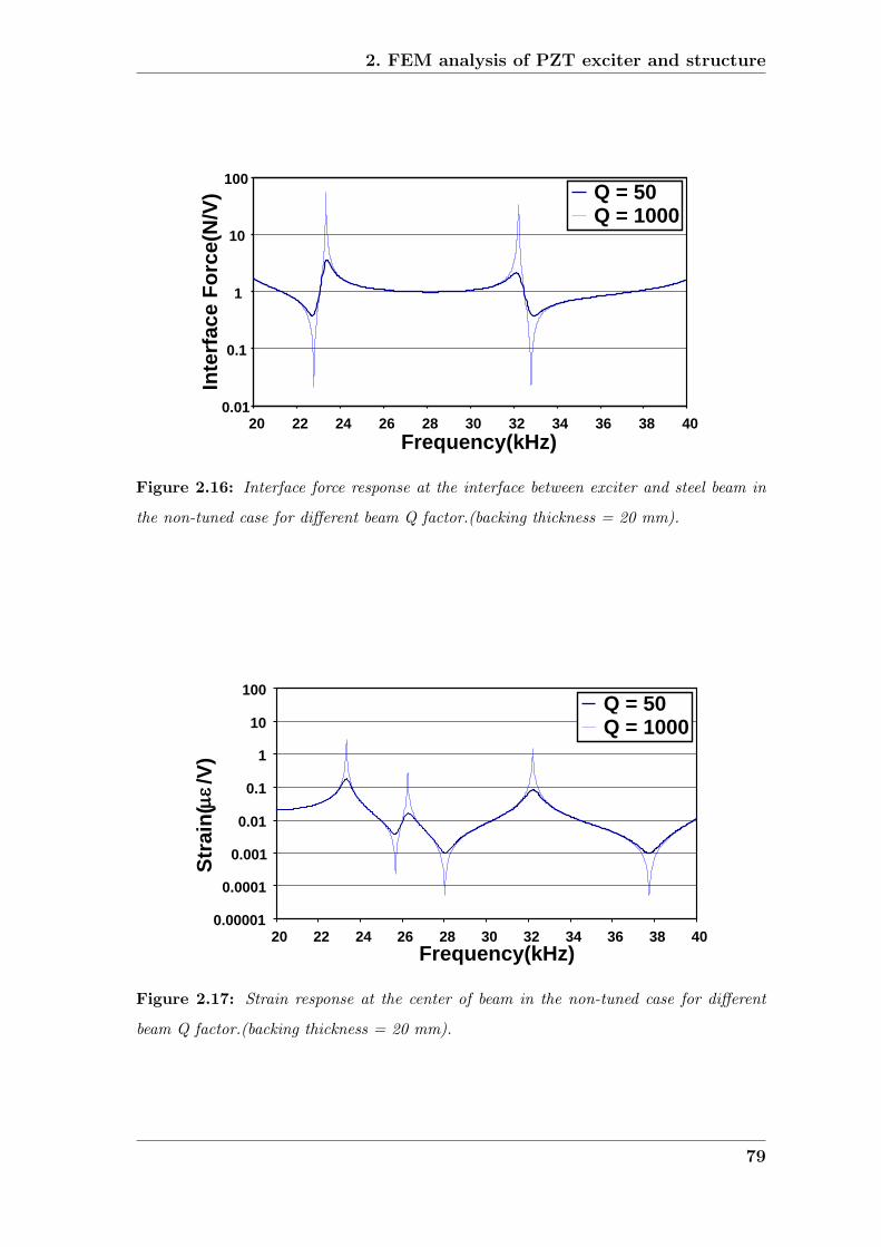
2. FEM analysis of PZT exciter and structure
0.01
0.1
1
10
100
20 22 24 26 28 30 32 34 36 38 40Frequency(kHz)
Inte
rfac
e Fo
rce(
N/V
) Q = 50Q = 1000
Figure 2.16: Interface force response at the interface between exciter and steel beam in
the non-tuned case for different beam Q factor.(backing thickness = 20 mm).
0.00001
0.0001
0.001
0.01
0.1
1
10
100
20 22 24 26 28 30 32 34 36 38 40Frequency(kHz)
Stra
in(με /
V)
Q = 50Q = 1000
Figure 2.17: Strain response at the center of beam in the non-tuned case for different
beam Q factor.(backing thickness = 20 mm).
79
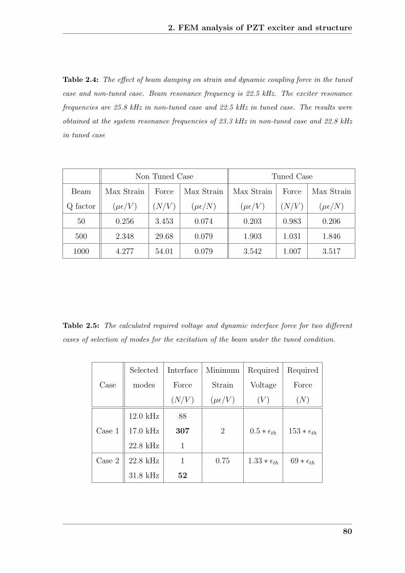
2. FEM analysis of PZT exciter and structure
Table 2.4: The effect of beam damping on strain and dynamic coupling force in the tuned
case and non-tuned case. Beam resonance frequency is 22.5 kHz. The exciter resonance
frequencies are 25.8 kHz in non-tuned case and 22.5 kHz in tuned case. The results were
obtained at the system resonance frequencies of 23.3 kHz in non-tuned case and 22.8 kHz
in tuned case
Non Tuned Case Tuned Case
Beam Max Strain Force Max Strain Max Strain Force Max Strain
Q factor (µε/V ) (N/V ) (µε/N) (µε/V ) (N/V ) (µε/N)
50 0.256 3.453 0.074 0.203 0.983 0.206
500 2.348 29.68 0.079 1.903 1.031 1.846
1000 4.277 54.01 0.079 3.542 1.007 3.517
Table 2.5: The calculated required voltage and dynamic interface force for two different
cases of selection of modes for the excitation of the beam under the tuned condition.
Selected Interface Minimum Required Required
Case modes Force Strain Voltage Force
(N/V ) (µε/V ) (V ) (N)
12.0 kHz 88
Case 1 17.0 kHz 307 2 0.5 ∗ εth 153 ∗ εth22.8 kHz 1
Case 2 22.8 kHz 1 0.75 1.33 ∗ εth 69 ∗ εth31.8 kHz 52
80

2. FEM analysis of PZT exciter and structure
25.5 kHz 27.7 kHz
29.2 kHz 30.1 kHz
Figure 2.18: Coupled system mode shapes of steel plate(300× 300× 5mm).
0.00E+00
5.00E-07
1.00E-06
1.50E-06
2.00E-06
2.50E-06
3.00E-06
3.50E-06
4.00E-06
0 50 100 150 200 250 300X(mm)
Stra
in( ε
/V)
ε11 ε22 ε33ε12 ε13 ε23
Figure 2.19: Strain components along the centreline of the beam (300× 20× 20mm) at
22.8 kHz. X is the length of the beam.
81
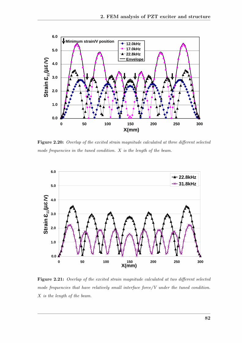
2. FEM analysis of PZT exciter and structure
0.0
1.0
2.0
3.0
4.0
5.0
6.0
0 50 100 150 200 250 300X(mm)
12.0kHz17.0kHz22.8kHzEnvelope
Minimum strain/V positionSt
rainε 1
1(με
/V)
Figure 2.20: Overlap of the excited strain magnitude calculated at three different selected
mode frequencies in the tuned condition. X is the length of the beam.
Stra
inε 1
1(με
/V)
0.0
1.0
2.0
3.0
4.0
5.0
6.0
0 50 100 150 200 250 300X(mm)
22.8kHz31.8kHz
Figure 2.21: Overlap of the excited strain magnitude calculated at two different selected
mode frequencies that have relatively small interface force/V under the tuned condition.
X is the length of the beam.
82

Chapter 3
Experimental study with PZT
exciter
The purpose of this chapter is to evaluate different excitation systems with a PZT
exciter for constructing a more practical and convenient excitation system for ther-
mosonic testing. Therefore, an experimental investigation of the performance of
PZT exciters and the different coupling methods was conducted. The tests were
conducted on steel beams, steel plates and composite plates. The experimental
setup is described and tests conducted on different structures with different cou-
pling methods are reported in this chapter.
3.1 Test Setup
Investigations of the performance of different PZT exciters were conducted by eval-
uating the excited strain in the structures and the dynamic interface force between
the exciter and structure. Figure 3.1 shows the apparatus used in the tests on steel
beams, steel plates and composite plates. The PZT exciter was operated by the
amplified output signal from a frequency response analyser (SOLARTRON 1255).
An ENI amplifier or WAVEMAKER amplifier with a dial that can provide a conve-
nient way in controlling output voltage from the amplifier was used as an amplifier
83

3. Experimental study with PZT exciter
for supplying power to the PZT exciter.
The strain was measured by a semi-conductor type strain gage and the strain signal
was sent to the frequency response analyser via strain gage amplifier(FYLDE FE-
527-SGA) which has a cut off frequency of 50 kHz. Therefore, above 50 kHz, the
measured strain signal was attenuated. If accurate strain values above 50 kHz are
required, amplitude compensation by gains calculated from the frequency response
of strain amplifier is required. The dynamic interface force was measured by a
force gage (B&K 8200) assembled on the PZT exciter as shown in Figures 3.1 and
3.3(a)(b). The force signal was sent to the FRA via a conditioning amplifier (B&K
2626). The FRA gave the frequency response from the measured strain and force
signals.
The force gage (B&K 8200) has a frequency response characteristic shown in Figure
3.2. The force transducer frequency response is defined as [83]:
R(ω) =FoFt
(3.1)
where R(ω) denotes the response at a frequency ω, Fo is the measured force which
is acting on the piezoelectric discs in the force transducer and Ft is the actual
force between exciter and specimen. The measured force is smaller than the actual
force at frequencies above 20 kHz as shown in the curve in Figure 3.2. Therefore,
the magnitude of the force measured at different frequencies should be carefully
compared considering this characteristic. However, it can be effectively used for the
comparison of the force measured at similar frequencies and for obtaining the force
response characteristics. The mass of the force gage below the sensing elements
leads to an error in the measured structural response characteristics since the force
required to accelerate the mass is measured but is not transmitted to the structure.
The manufacturer attempts to reduce this error by minimizing the mass of this part
of the gage [69].
84

3. Experimental study with PZT exciter
3.2 Vibrational characteristics of the PZT exciter
Figure 3.3 shows three different PZT exciters used for the following tests on steel
plates and composite plates. Exciter 1 and Exciter 2 have a force gauge in order to
obtain the level of the dynamic interface force and investigate the frequency response
of the interface force. Ring type Pz26 elements with 20mm outer diameter and 5mm
inner diameter were used for the exciters and a brass shim was used as an electrode.
Exciter 1 has a backing block composed of four different square steel blocks (one
10mm thick block and three 2mm thick blocks) bonded together as shown in Figure
3.3(a). This exciter was originally made for the investigation of the influence of
backing thickness on the exciter resonance frequency. In this thesis the effect of
the different assembly methods for the Exciter 1 and the Exciter 2 on the obtained
strain level will be discussed in section 3.3.3. Exciter 2 has a single solid backing
block as shown in Figure 3.3(b). The backing block, PZT elements and the force
gage are clamped together without adhesive using a nut and a bolt. The force gage
also has a threaded stud (M5) at the end of the gage as shown in Figure 3.3(a) that
can be used to couple the exciter to a tested structure. A magnet could be used to
give the coupling force in certain cases. Therefore, an exciter was fabricated with a
magnet replacing one of the steel end blocks. The magnet in the exciter shown in
Figure 3.3(c) is longer than the other end block so the PZT elements are no longer
in the middle of the exciter. This will reduce the output of the exciter but the longer
magnet will give a greater clamping force.
Figure 3.4 shows velocity responses of the three different exciters under a 20Vpp
input voltage condition. A schematic of the measurement method for the vibrational
velocity of the exciters is also shown in Figure 3.4. Each exciter has a different
resonance frequency because of the different lengths and materials. Table 3.1 shows
the exciter total lengths and the resonance frequencies of the exciters. The Q factors
in Table 3.1 were calculated by the half power point method from the test results
under the 20Vpp input voltage condition in Figure 3.4. Table 3.1 shows that Exciter
1 has higher damping than Exciter 2. This is probably due to the larger number of
interfaces in this exciter. The exciter with the magnetic base also show low Q factor.
85

3. Experimental study with PZT exciter
This seems to be caused by thicker bonding layers and the material damping of the
magnet. Figure 3.5 shows a comparison of the measured velocity of different exciters
as a function of input voltage. The velocity was measured by laser vibrometer at
the end surface of the exciter. Generally, the velocity is proportional to the input
voltage. However, the three exciters show different performance at the same voltage
input level. Comparison of Figure 3.5 and Table 3.1 shows the close relationship
between the vibration velocity and Q factor. Therefore it can be concluded that
high Q of the exciter is required to obtain higher excitation per unit voltage input.
It will be shown in section 3.3.3 that exciter 2 excites higher strain per unit input
voltage than exciter 1 in the steel plate tests.
3.3 Frequency response of beam and plate
3.3.1 Frequency response of steel beam
The force frequency response and the strain frequency response of a beam were
measured by using the same test set up as shown in Figure 3.1. Initially, an impact
test was conducted to find resonance frequencies of a beam. Figure 3.6 shows a
schematic of the test method. The beam is 300 mm in length, 20 mm in thickness
and 20 mm in width. The beam was supported on a very thin fishing line at two
arbitrary positions. Excitation was provided by dropping a 3mm steel ball onto
the beam. The vibration of the beam was monitored with a laser vibrometer, and
the resulting signal was passed to Imperial College software, SPECTRUM, via an
oscilloscope (LeCroy 9310A). Figure 3.6 shows the measured mode frequencies of
the beam up to 50 kHz.
Tuning an exciter to one of the beam mode frequencies makes it possible to excite a
beam with small dynamic interface force. However, there is a difficulty in fabricating
a tuned exciter on a beam as discussed in section 2.3.4. Therefore, three exciters
with resonance frequencies close to one of the beam mode frequencies were fabricated
and used to investigate the frequency response characteristic of the interface force
86

3. Experimental study with PZT exciter
and the excited strain in a beam. The exciters were made by changing the thickness
of backing block with different length of square steel section. These exciters were
similar to exciter 1 in Figure 3.3(a) except that they were clamped by a stud and
a nut without bonding. Figure 3.7 shows the velocity responses of the 3 different
exciters. They have different resonance frequencies and vibration magnitude at the
resonances.
Tests were conducted to observe the effect of the attachment of a PZT exciter on
the frequency response and to compare the frequency responses produced by the
three different exciters with different resonance frequencies near one of the beam
mode frequencies. In this case, the selected beam mode frequency of interest is 21.6
kHz. The exciter was coupled by a stud in the end of the force transducer that was
assembled into the exciter as shown in Figure 3.3(a). The exciter was screwed into a
threaded hole at the center of the beam and the strain was measured at the center of
the reverse surface of the beam. Figure 3.8 shows the frequency responses with the
three different exciters shown in Figure 3.7. It is shown that generally the interface
force maximum occurs at the strain maximum and the interface force is a minimum
near the flexural mode frequency of the beam itself. Figure 3.9 and Figure 3.10 show
the force response and the strain response of the beam around 21.6 kHz which is the
7th flexural mode frequency of the beam. The force is a minimum at 21.6 kHz near
the beam mode frequency of 21.6 kHz but the strain maximum frequency is different
from the beam mode frequency. The strain maximum frequency of the coupled
system is affected by the exciter resonance frequency and beam mode frequency as
predicted in the numerical study in section 2.3.1 and the excited strain becomes
larger near the exciter resonance frequency. Table 3.2 shows a comparison of the
test results obtained by the three different exciters used in the tests shown in Figures
3.8-3.10. As shown in Figure 3.7, each exciter shows different vibration amplitude at
resonance. Therefore, direct comparison of the strain and the force at the different
frequencies is difficult. However, it can be concluded from the results in Table 3.2
that if an exciter resonance frequency approaches a beam mode frequency, the strain
per unit interface force increases as would be expected.
87

3. Experimental study with PZT exciter
Figure 3.11 shows the force response and the strain response of the steel beam
obtained with exciter 2 shown in Figure 3.3(b). The frequency of the maximum
strain is higher than those of the cases shown in Figure 3.8 because the resonance
frequency of exciter 2 is 31.2 kHz near the beam mode frequency of 31.3 kHz.
Figure 3.12 shows the measured system mode shapes of the steel beam obtained at
the resonances shown in Figure 3.11 during excitation with exciter 2 coupled with
a stud to the center of the beam and Figure 3.13 shows the predicted system mode
shapes of the steel beam obtained by using 3D FEM. Figures 3.12 and 3.13 were
calculated from the magnitude of the out of plane velocity along the centerline of
the steel beam. It can be seen in Figure 3.12 and Figure 3.13 that the measured
frequencies and mode shapes of 7th and 9th modes are very similar to the prediction.
This result shows that numerical predictions can provide the mode shapes and mode
frequencies of the coupled exciter-structure system in simple structures such as a
steel beam.
3.3.2 Frequency response of steel plate
For the case of the thick steel beam, the mode density is too low to obtain enough
modes around the exciter resonance frequency. However, structures of practical
interest tend to be more plate-like than beam-like and plates have a higher mode
density than beams. Therefore, square plates with different thicknesses were tested
to see the excitation performance of the PZT exciter. The side length of the plates is
300mm in this case. Figure 3.14 shows the tested plate with an exciter at the center
of the plate. Exciter 1 and 2 that were shown in Figure 3.3(a) and (b) were used for
these tests. Each exciter has a force transducer with a stud at the excitation end. To
avoid drilling a hole in the structure, a ring shaped aluminium connector was used
to locate the exciter at the center of the plate as shown in Figure 3.15. The force
gage was screwed into the connector that was bonded to the plate. The same torque
of 3 Nm was applied to assemble the exciter to the connector for tests on plates with
different thicknesses. Figure 3.3(a) shows exciter 1 without the aluminium connector
and Figure 3.3(b) shows the exciter 2 with the connector. An exciter was located
88

3. Experimental study with PZT exciter
at the center of the plate and the strain in one direction was measured at the center
of the reverse surface of the plate as shown in Figure 3.15. In the following tests,
strain in one direction parallel to the edge of the plate was measured as shown in
Figure 3.15.
Figure 3.16 shows the interface force response (N/V) of the 4mm thick steel plate
obtained by a sweep test with exciter 2. The force is small around the exciter 2
resonance frequency of 31.2 kHz in Figure 3.16. Figure 3.17 shows the response of
strain per unit voltage of the steel plate with 4mm thickness obtained in the same
test as shown in Figure 3.16. Several peaks are found around the exciter resonance
frequency in Figure 3.17. These results mean that several modes can be excited
around the exciter resonance frequency with small input voltage and small interface
force. More modes than those shown in Figure 3.17 probably exist because the
strain was measured in one direction so modes that have a small component in
the measurement direction are not seen. Figure 3.18 shows the response of strain
per unit interface force of the steel plate with 4mm thickness calculated from the
measured responses of force and strain in Figure 3.16 and Figure 3.17. Generally,
peaks in Figure 3.18 are found at the force anti-resonance frequencies. However, a
peak value is also found at the frequency of maximum strain per unit voltage of
32.3 kHz. Therefore, at this frequency high strain can be obtained with small input
voltage and small interface force. This frequency seems to be close to the tuned
condition discussed in section 2.3.2.
3.3.3 Frequency response of steel plates with different thick-
nesses
Figure 3.19 and Figure 3.20 show the test results obtained with exciter 1 that was
coupled to plates of different thicknesses as shown in Figure 3.15. Figure 3.21 and
Figure 3.22 show the corresponding test results obtained with exciter 2. Figure 3.19
and Figure 3.21 show the maximum strain measured at the center of the plate as
a function of the magnitude of input voltage. The maximum strain frequency was
89
3. Experimental study with PZT exciter
selected from the sweep test results such as Figure 3.17 where strain was measured
in one direction. Figure 3.20 and Figure 3.22 show the dynamic interface force at
the frequency of maximum strain as a function of the input voltage. Generally, the
strain is proportional to the input voltage. However, a saturation phenomenon was
observed in the test results in Figure 3.19. The saturation seems to be caused by
a non-linear softening spring characteristic of the bonding material. As the input
voltage increases, the displacement of the tip of the exciter tends to increase linearly
and hence it would be expected that the strain in the bond layer also increases
roughly linearly. However, the rate of increase of the dynamic interface force tends
to decrease as the voltage increases. This suggests that the bond layer has a softening
stiffness characteristic.
The influence of plate thickness on the excited strain and the interface force is
difficult to derive from the test results in Figures 3.19-3.22 because of different
tuning conditions in each plate. Figure 3.21 and Figure 3.22 show the test results
obtained with exciter 2. It is interesting that the excited strain is not inversely
proportional to the plate thickness. The 4 mm and 3 mm cases show a little higher
strain than the 2mm case in Figure 3.21. This is because the exciter is the same but
the tuning state is different in each plate because the different plates have different
modal characteristics. This characteristic is more evident in the results on the 4mm
plate that show a small dynamic interface force in Figure 3.22 but the strain shown
in Figure 3.21 is higher than the 2mm case and similar to the 3mm case which shows
the highest interface force in Figure 3.22. This suggests that the 4mm thickness case
is close to the tuned state where the plate resonance frequency coincides with the
exciter resonance frequency.
It is also concluded from the results that exciter 2 excites more strain than exciter 1
regardless of plate thickness. The larger number of bonding layers in exciter 1 causes
higher damping in exciter 1 for which the Q factor is 25 compared with exciter 2
which has a Q factor of 123 as shown in Table 3.1; we can see from this result that
damping of an exciter is one of the dominant factors affecting the excited strain.
90
3. Experimental study with PZT exciter
3.4 The performance of different coupling meth-
ods
3.4.1 Comparison of the performance of different coupling
methods
An exciter for thermosonics should be easy to attach to and remove from the struc-
ture. If a small exciter is used and the dynamic interface force between the exciter
and the structure is small, coupling materials such as wax or tape could be used to
fix the exciter on the structure. Therefore different coupling methods were investi-
gated experimentally. In this study, rigid bonding with adhesive, wax and double
side tape were tested and compared. Figure 3.23 and Figure 3.24 show the test
results obtained by exciter 2 in Figure 3.3(b) on a 5mm thick plate. The strain in-
creases with the input voltage but it is not linear and a saturation phenomenon was
observed especially in the tape coupling case. The saturation seems to be caused
by a softening spring characteristic of the coupling material. This softening char-
acteristic causes the saturation of the interface force and the strain as discussed in
section 3.3.3. From the electrical point of view, the degree of impedance matching
also affects the performance of the exciter and the excited strain in the tested struc-
ture. However, the results in Figure 3.23 and Figure 3.24 were obtained with the
same exciter and power supply system on the same plate. Therefore, the different
saturation characteristics between different coupling materials seem to be mainly
caused by the different characteristics of the coupling materials. In the bonding
case, the strain has a nearly linear relationship with the input voltage. The strain
in the bond case is similar to that with wax but the force is much smaller. These
results seem to be caused by different tuning conditions and damping characteristics
of the coupling materials. The measured Q factors of strain responses at the strain
maximum frequencies are 1,689 for the bond case, 963 for the wax, and 1,141 for
the tape at the 125 V input condition. Though wax has higher damping than the
bond, the interface force is much larger in the wax case than the bond case. This is
91

3. Experimental study with PZT exciter
probably a result of different tuning conditions which seem to be caused by different
stiffnesses of the three different coupling materials.
In conclusion, a saturation characteristic in strain and force is observed in the tape
case and this seems to be mainly caused by the softening characteristic of the
tape. The results show that enough strain can be obtained with small PZT ex-
citers through coupling materials such as wax and tape for applications that require
small strain levels in thermosonic tests.
Figure 3.25 shows the FFT of the input voltage, dynamic interface force and strain
signal measured on the 4 mm plate with wax coupled exciter 2. These signals were
measured when the exciter was operated at 31.1 kHz, that is at the frequency of
the maximum strain found in a sweep test in the wax coupling case under the 125
V input voltage condition. The FFT was conducted by the SPECTRUM software.
The strain signal was attenuated in the frequency range above 50 kHz because the
cut off frequency of the strain gage amplifier is 50 kHz. The force signal was also
attenuated in the high frequency range above 30 kHz because of the characteristic
of the force transducer as shown in Figure 3.2. However, the FFT of the signal can
be used to check the existence of high frequency harmonic and low frequency sub-
harmonic components of the excitation frequency that provide evidence of non-linear
vibration. As discussed in the earlier section, severe non-linear vibration caused by
hammering of the exciter should be avoided to obtain reproducible and reliable
excitation. In other words, if an exciter excites at single frequency, the strain signal
measured in the tested structure should also have a single frequency component.
Figure 3.25 shows that there is no sub harmonic component. There are harmonics
in the response but they are also present in the input voltage. The first harmonic
in the input was -20dB compared to the fundamental and the first harmonic in the
strain was also -20dB compared to the fundamental. This suggests that the wax
coupling did not introduce further non-linearity. A similar frequency characteristic
was obtained in the bond case.
Figure 3.26 shows the FFT of input voltage, dynamic interface force and strain
signal measured on the 5mm plate with tape coupled exciter 2. This results shows
92

3. Experimental study with PZT exciter
an example of non-linear vibration. These signals were measured when the exciter
was operated at 33.2 kHz at 125V at which a hammering noise was generated during
the test. This input voltage level seems to cause the dynamic interface force to
reach the bond strength limit of tape coupling and loss of contact to start. The
input voltage signal just shows harmonics of input voltage frequency as in Figure
3.25 but the dynamic interface force and the strain signals show typical non-linear
vibration characteristics including harmonic and sub harmonic components of the
excitation frequency. It is interesting that the signal is non-linear but the maximum
magnitude appears at the excitation frequency. This does not always happen with
the non-linear vibration as discussed in Chapter 5.
3.4.2 The performance of magnetic coupling
The exciter with a magnet block shown in Figure 3.3(c) was tested on the steel plates.
A magnet may be one of the possible coupling options for some metal structures.
The results in Figure 3.27 were obtained from 5mm and 4mm thickness plates.
The strain is higher in the 4mm case than the 5mm case. Generally, the strain is
proportional to the input voltage but a saturation phenomenon was observed at high
input voltage. 19 µε was obtained at an input voltage of 125V in the 4mm plate case.
It should also be kept in mind that the tuning state is different in each plate case in
Figure 3.27. The strain level obtained using the exciter with the magnetic base is
much lower than the strain level obtained with wax coupled exciter 2, which was 73
µε on the 4mm thick steel plate and 55 µε on the 5mm thick steel plate at an input
voltage of 125V. The reduced strain levels with the magnetic exciter are probably
largely due to the high damping of the exciter, and this could probably be reduced
if necessary; strain levels over 50 µε are often required in metal structures [14].
93

3. Experimental study with PZT exciter
3.5 Test of composite plate
3.5.1 Frequency response of composite plate
The frequency response characteristics of relatively high damping materials such
as composites are different from steel structures. An angle-ply (45/0/-45) carbon
fiber reinforced plastic(CFRP) composite plate was tested using exciter 2. The
plate was 150 mm in length, 100 mm in width and 7 mm in thickness. The exciter
was coupled by wax and located at the center of the plate and the strain in one
direction was measured at the center of the reverse surface of the plate as shown
in Figure 3.28. Figure 3.28 shows the maximum strain measured at the center of
the plate as a function of the magnitude of input voltage and Figure 3.29 shows the
dynamic interface force at the frequency of maximum strain obtained in the same
test as shown in Figure 3.28. It was seen that the dynamic interface force and the
strain level are much lower than those obtained in the steel plate test case with the
same exciter. It is also observed that the wax coupling is consistent and the strain
obtained at 125 V is about 8 µε. According to the results obtained by Barden et
al [45], the required strain level is below 10 µε for the same type of CFRP composite
plate. Therefore, this strain level is sufficient for the thermosonic test.
Figures 3.30 and 3.31 show the frequency response functions of strain and interface
force per unit input voltage obtained during a sweep test on the composite plate
with exciter 2 under the 10V input voltage condition. At 125V input voltage some
loss of contact at the maximum force frequency during the sweep test was observed.
Therefore, a relatively low voltage of 10V was used to obtain the frequency responses.
The maximum force frequency of 31.2 kHz is different from the maximum strain
frequency of 29.5 kHz and the force at the maximum strain frequency is much
smaller than the maximum force. The measured strain response shows broad peaks
at the resonances because of the higher damping characteristic of the composite
plate. The Q factor obtained at the maximum strain frequency in Figure 3.30 is 23.
This value is much smaller than the 655 obtained in the 4mm thickness steel plate
test with the same wax coupled exciter. Generally, the excited strain and dynamic
94
3. Experimental study with PZT exciter
interface force are smaller than the steel plate case.
3.5.2 Thermosonic test of composite plate
Barden et al [45] show that surface temperature rise is inversely proportional to ther-
mal conductivity. Thus for the same energy released at the defect the temperature
rise in CFRP is about 50 times more than in mild steel because CFRP has a thermal
conductivity about 50 times lower than a mild steel. In metals, the energy is diffused
away from the defect fast and the temperature rise saturates after a few seconds.
As a consequence a pulse length of more than a few seconds would not lead to a
significant increase in surface temperature. In composites, the heat is trapped near
the defect and the surface temperature rise increases over a longer time. Therefore
for CFRP there are advantages to increasing the pulse time [45]. If the pulse time is
increased the same surface temperature rise can be obtained with less power being
released at the defect. Lowering the power of the horn will reduce the heating at the
horn tip so the surface is not damaged and less vibration will reduce the chance of
fretting and chattering. Another advantage of the low power requirement for long
pulse thermosonics is that it is possible to develop a lightweight portable system
such as a simple PZT exciter. Therefore, the performance of a simple PZT exciter
as an exciter for thermosonic testing was investigated.
The exciter used in the previous section is exciter 2 which has a resonance frequency
of 31.2 kHz. But a simple PZT exciter with a higher resonance frequency could be
used to excite the structure with sufficient response at high frequency which leads to
the higher temperature rise at the surface because the heating rate is proportional
to excitation frequency. Therefore, a simple PZT exciter with higher resonance fre-
quency of 49.2 kHz and 20mm diameter and 30mm overall length was manufactured
as shown in Figure 3.32 and used in thermosonic testing. Figure 3.32(b) illustrates
the construction of the exciter, in which piezoelectric elements are sandwiched be-
tween two steel blocks which have a M5 threaded hole and clamped with a M5
bolt. A brass shim was used as an electrode in this exciter. Figure 3.33 shows the
maximum strain measured at the center of the composite plate as a function of the
95

3. Experimental study with PZT exciter
magnitude of input voltage when it was excited by the simple PZT exciter shown in
Figure 3.32, which was coupled to the plate by wax. 20 µε was obtained at the 100
V input voltage condition. According to the results obtained by Barden et al [45],
this strain level is sufficient for the thermosonic test of CFRP composite structures.
Barden et al [45] show that composite could be tested at low strain levels below 10
µε by increasing the excitation time and observing the temperature increase towards
the end of the excitation time.
A thermosonic test was conducted on the same type of composite plate with barely
visible impact damage produced by a 26 J impact that was supplied by Professor
Darryl Almond at Bath University. Figures 3.34(a),(b) and (c) show the front
surface, the rear surface and the measured C-scan image of the damage in the
tested composite plate respectively. The impact site was at the center of the rear
surface and the PZT exciter operated at 100 V input voltage was located close to
the edge of the plate at the front surface as shown in Figure 3.34(d),(e) and (f).
An IR camera (CEDIP) with temperature threshold value of 30mK and 320 × 240
pixels recorded the thermal image at the front surface at a frame rate of 10 Hz. The
recorded thermal images at different times are shown in Figures 3.34(d), (e) and (f).
Figure 3.34 shows test results obtained on the CFRP composite plate; these images
are raw data images not processed by a background image substraction. As the
excitation time increases, the temperature rise at the damage area increases and
the thermal image becomes clearer as shown in Figures 3.34(d), (e) and (f). The
coupling was consistent and there was no impact problem caused by a loss of contact
between the exciter and the plate.
It was also observed that the temperature rise at the interface between the exciter
and the composite plate was not high enough to cause damage at the interface.
Figure 3.35 shows the maximum temperature rise at the damage area and the area
adjacent to the PZT exciter. As the excitation time increases, the temperature rise
at the damage area and near the exciter increases gradually with the exception that
the interface temperature shows a change of the slope at 25 sec, which is probably
caused by a change in the wax coupling. The temperature rise at the damage
96

3. Experimental study with PZT exciter
area is 1.44K after a 50sec excitation and the temperature rise near the interface
is 0.93K after a 50sec excitation in the same test. The obtained temperature rise
in the damage area is much higher than the camera sensitivity of 30mK and this is
adequate for the thermal image to be clearly observed. The result shows that the
simple PZT exciter can be used on composite plates.
Generally, a short pulse whose pulse duration is below 1 sec has been used to excite
metal structures for thermosonics but in composite structures a longer pulse time
is better for obtaining larger temperature rise around a damage, which helps the
infrared camera to detect the damage more clearly as shown in Figures 3.34(d), (e)
and (f). The test time of 10 to 15 seconds is comparable to flash and pulse optical
thermography, as all thermographic methods are limited by the rate of thermal
diffusion within the material [45]. It may be possible to reduce the excitation time
for thermosonics by increasing the power, but the method will be limited by the
thermal properties of CFRP.
3.6 Review of Chapter
The purpose of this chapter is to evaluate the different PZT exciters for constructing
a more practical and convenient excitation system for thermosonic testing.
An exciter for thermosonics should be easy to attach to and remove from the struc-
ture. If the dynamic interface force between the exciter and the structure is small, a
simple coupling such as wax and tape could be used to fix the exciter on the struc-
ture. The response obtained is linear with applied input voltage until the dynamic
force approaches the limit of the coupling strength; evidence of non-linear vibra-
tion was seen at higher input voltages. A saturation characteristic in strain and
force was observed with tape coupling and this seems to be caused by the softening
stiffness characteristic of the coupling material where the tape bond is likely to be
approaching failure.
Structures of practical interest tend to be more plate-like than beam-like and have
97

3. Experimental study with PZT exciter
high modal density and this high modal density can provide a large number of
resonances around the exciter resonance frequency and a high strain response at
several frequencies. The small interface force between the exciter and the structure
around the exciter resonance frequency reduces the possibility of surface damage
produced by chattering and tends to produce reproducible, single mode vibration.
However, if only one mode is excited, it is necessary to do another test at a different
frequency in order to ensure that sufficient strain is produced at all possible damage
sites and the excitation level for reliable defect detection is dependent on the strain
mode shapes of the selected modes.
The higher damping in composite plates causes a smaller dynamic interface force
and smaller excited strain than the steel plate. However, this strain level was suffi-
cient for the thermosonic test and impact damage was successfully detected by using
a simple PZT exciter. This thermosonic test result has shown that a simple, small
PZT exciter may provide a convenient, reliable thermosonic test system in applica-
tions such as composite structures where relatively low strain levels are required for
damage detection.
If it is intended to use reproducible vibration for reliable thermosonic testing, suffi-
cient strain levels should be achieved in the test structure before the interface force
reaches the limit value that causes loss of contact between the exciter and the test
structure. The strain level obtained using a wax coupled simple PZT exciter was 73
µε on a 4mm thick steel plate and 55 µε on a 5mm thick steel plate at an input volt-
age of 125V. These results show that a reproducible vibration may be sufficient for
thermosonic testing in some metal structures such as a thin plates. However strain
levels over 50 µε are often required in metal structures [14], though the required
strain level is dependent on the crack size. This level of strain is not easily achieved
within the reproducible vibration range because the interface force limit is reached
first. Therefore, the following studies are conducted with an acoustic horn with high
power capability to investigate the characteristics of the vibration produced in a real
structure with complex geometry and to develop an excitation method for achieving
reliable excitation in the non-linear vibration range.
98

3. Experimental study with PZT exciter
SOLARTRON
Frequency Response Analyzer
Power Amplifier
PC
Strain Amplifier
Strain Gage
Force Transducer
B&K 8200
Charge Amplifier
Input voltage
force
strain
( Semi Conductor Type)
Beam or Plate
Figure 3.1: Schematic of test set-up
20102 1005051 kHz500200
0
-10
10
dB
Figure 3.2: Calibration chart for Force-Transducer Type 8200
Table 3.1: Characteristics of three different exciters.
Exciter Type Exciter1 Exciter2 Magnet
Q factor 25 123 18
Total Length(mm)(except stud) 48 54 55
Resonance Frequency(Hz) 33795 31200 25400
99

3. Experimental study with PZT exciter
(c)
(a) (b)
Magnet(25mm thick)
Steel Block(10mm thick)
PZT Elements (20mm thick)
Bolt(M5)
Nut
20
Force Gage
Stud(M5)
Bonded Square Steel Blocks
PZT Elements (20mm thick)
20
Force Gage
AluminiumConnector
Steel Block(20mm thick)
Nut
Bolt(M5)
PZT Elements (20mm thick)
Figure 3.3: Three different exciters used for the tests in this study; (a) Exciter 1. Backing
block is composed of one 10mm thick square steel block and three 2mm thick square steel
blocks (b) Exciter 2 (c) Exciter with magnetic base.
05
101520253035404550
22 24 26 28 30 32 34 36Frequency(kHz)
Velo
city
(mm
/s)
Exciter 1
Exciter 2
Magnet
Laser Vibrometer
V
Figure 3.4: Velocity responses of three different exciters shown in Figure 3.3.
100

3. Experimental study with PZT exciter
00.05
0.10.15
0.20.25
0.30.35
0.40.45
0.5
0 50 100 150 200 250Input Voltage(V)
Velo
city
(m/s
)Exciter 2
Exciter 1
Magnet
25 50 10075 125
Figure 3.5: Vibrational velocity of three different exciters shown in Figure 3.3 at different
input voltages
0
50
100
150
200
250
300
350
400
450
0 10 20 30 40 50Frequency(kHz)
Velo
city
(Arb
itrar
y Sc
ale)
17074 Hz21598 Hz
26413 Hz
31334 Hz
12802 Hz
Laser Vibrometer
Impact
Figure 3.6: Mode frequencies of the beam.
101

3. Experimental study with PZT exciter
Table 3.2: Comparison of the test results obtained by different exciters on the steel beam.
Exciter Strain Max Strain Interface Strain/Force
Resonance Frequency Max Force (µε/N)
Frequency(kHz) (kHz) (µε/V ) (N/V )
18.7 21.1 0.16 1.27 0.13
20.4 21.4 0.26 0.63 0.42
21.1 21.6 0.45 0.67 0.67
0
5
10
15
20
25
30
35
40
10 12 14 16 18 20 22 24 26 28 30Frequency(kHz)
Velo
city
(mm
/s)
E18.7E20.4
E21.1
Figure 3.7: The velocity responses of 3 different exciters under the 32Vpp input condition.
The subscripts refer to the resonance frequencies in Table 3.2
102

3. Experimental study with PZT exciter
1E-11
1E-09
1E-07
1E-05
0.001
0.1
10
1000
10 12 14 16 18 20 22 24 26 28 30Frequency(kHz)
Stra
in( ε
/V)
(N/V
)Force(N/V)
Strain(ε/V)
E18.7
E20.4
E21.1
E18.7
E20.4 E21.1
Figure 3.8: The frequency responses of a beam with three different exciters whose re-
sponses are shown in Figure 3.7.(Beam 200×20×20mm).
0.001
0.01
0.1
1
10
18 19 20 21 22 23 24
Frequency(kHz)
Inte
rfac
e Fo
rce(
N/V
)
E18.7
E20.4
E21.1
21570 Hz Beam Mode Frequency21598 Hz
Figure 3.9: Interface force response near the beam mode frequency of 21598 Hz.
103

3. Experimental study with PZT exciter
0.001
0.01
0.1
1
18 19 20 21 22 23 24Frequency(kHz)
Stra
in( με/
V)E18.7
E20.4E21.1
Beam Mode Frequency21598 Hz
Figure 3.10: Strain response near the beam mode frequency of 21598 Hz.
20 25 30 35 40
0.001
0.01
0.1
1
Force(N/V)
Strain(με/V)
Frequency(kHz)
Stra
in(με /
V)
0.01
0.1
1
10
100
Interface Force(N/V)
Figure 3.11: The frequency responses of the steel beam(200×20×20mm) obtained with
exciter 2.
104

3. Experimental study with PZT exciter
0
0.2
0.4
0.6
0.8
1
1.2
0 50 100 150 200 250 300X(mm)
Nor
mal
ized
Am
plitu
de
Measured Mode Shape
(laser scanning)
Exciter resonance : 31.7kHz(Bolt Coupling)
22.0kHz(7th) 31.4kHz(9th)
Figure 3.12: Measured mode shapes of the steel beam(200×20×20mm) obtained during
the excitation with the exciter 2 coupled with a stud at the center of the beam. Exciter
resonance frequency is 31.2 kHz. X is the length of the beam.
0
0.2
0.4
0.6
0.8
1
1.2
0 50 100 150 200 250 300X(mm)
Nor
mal
ized
Am
plitu
de
Measured Mode Shape
(laser scanning)
Exciter resonance : 31.7kHz(Bolt Coupling)
22.8kHz(7th) 31.8kHz(9th)
Figure 3.13: Predicted mode shapes of the steel beam(200×20×20mm) obtained by using
a 3D FEM. Exciter resonance frequency is 22.5 kHz. X is the length of the beam.
105

3. Experimental study with PZT exciter
Figure 3.14: Test Set-up for plate
Force Transducer
Ring shaped aluminium connector
Steel Plate Strain Gage
300
300
Strain measurement direction
(b) Plan View
(a) Side View
Figure 3.15: Attachment method of exciter used in plate tests.
106

3. Experimental study with PZT exciter
0
2
4
6
8
10
12
14
20 22 24 26 28 30 32 34 36 38 40Frequency(kHz)
Inte
rfac
e Fo
rce/
Volt(
N/V
) Exciter Resonance Frequency
Figure 3.16: Force response (N/V) of the steel plate of 4 mm thickness excited by Exciter
2.
0
0.1
0.2
0.3
0.4
0.5
0.6
0.7
0.8
0.9
20 22 24 26 28 30 32 34 36 38 40Frequency(kHz)
Stra
in/V
olt( με/
V)
Exciter Resonance FrequencyMaximum Strain at 32.3 kHz
Figure 3.17: Strain (µε/V ) response of the steel plate of 4 mm thickness excited by
Exciter 2.
107

3. Experimental study with PZT exciter
0
1
2
3
4
5
6
7
8
9
20 22 24 26 28 30 32 34 36 38 40
Frequency(kHz)
Stra
in/F
orce
( με/
N)
Exciter Resonance Frequency
32.3 kHz
Figure 3.18: Strain (µε/N) response of the steel plate with 4 mm thickness excited by
Exciter 2.
108

3. Experimental study with PZT exciter
0
5
10
15
20
25
30
35
40
0 20 40 60 80 100 120 140Input Voltage(V)
Stra
in( με) t4
t3
t5
t2
Figure 3.19: The maximum strain excited by exciter 1 on plates of different thickness as
a function of the magnitude of input voltage. t2: 2 mm thick plate, t3: 3 mm thick plate,
t4: 4 mm thick plate, t5: 5 mm thick plate
0
20
40
60
80
100
120
140
160
0 20 40 60 80 100 120 140Input Voltage(V)
Inte
rfac
e Fo
rce(
N)
t4
t3
t5
t2
Figure 3.20: The dynamic interface force at the frequency of maximum strain on plate of
different thickness as a function of the magnitude of input voltage. t2: 2 mm thick plate,
t3: 3 mm thick plate, t4: 4 mm thick plate, t5: 5 mm thick plate
109

3. Experimental study with PZT exciter
0
10
20
30
40
50
60
70
80
90
0 20 40 60 80 100 120 140Input Voltage (V)
Stra
in ( μ
ε)t4t3
t5t2
Figure 3.21: The maximum strain excited by exciter 2 on plates of different thickness as
a function of the magnitude of input voltage. t2: 2 mm thick plate, t3: 3 mm thick plate,
t4: 4 mm thick plate, t5: 5 mm thick plate
0
20
40
60
80
100
120
140
160
0 20 40 60 80 100 120 140Input Voltage(V)
Inte
rfac
e Fo
rce(
N)
t4
t3
t5
t2
Figure 3.22: The dynamic interface force at the frequency of maximum strain on plate of
different thickness as a function of the magnitude of input voltage. t2: 2 mm thick plate,
t3: 3 mm thick plate, t4: 4 mm thick plate, t5: 5 mm thick plate
110

3. Experimental study with PZT exciter
0
10
20
30
40
50
60
0 20 40 60 80 100 120 140
Input Voltage (V)
Stra
in ( με)
WAX
BOND
TAPE
Figure 3.23: the maximum strain excited in the 5 mm plate as a function of the magnitude
of input voltage for different methods of attachment
0
50
100
150
200
250
0 20 40 60 80 100 120 140Input Voltage(V)
Inte
rfac
e Fo
rce(
N)
WAX
BOND
TAPE
Figure 3.24: the dynamic interface force at the frequency of maximum strain in the 5 mm
plate as a function of the magnitude of input voltage for different methods of attachment.
111

3. Experimental study with PZT exciter
0.01
0.1
1
10
100
1000
10000
0 0.02 0.04 0.06 0.08 0.1 0.12 0.14 0.16 0.18 0.2
Frequency(MHz)
Arb
itrar
y
Strain
0.01
0.1
1
10
100
1000
0 0.02 0.04 0.06 0.08 0.1 0.12 0.14 0.16 0.18 0.2
Frequency(MHz)
Arb
itrar
y
Interface Force
0.01
0.1
1
10
100
1000
10000
0 0.02 0.04 0.06 0.08 0.1 0.12 0.14 0.16 0.18 0.2
Frequency(MHz)
Arb
itrar
y
Input Voltage
Figure 3.25: FFT of input voltage, dynamic interface force and strain signal measured
on the 4 mm plate with wax coupled exciter 2. Input voltage is 125 V.
112

3. Experimental study with PZT exciter
0.01
0.1
1
10
100
1000
10000
0 0.02 0.04 0.06 0.08 0.1 0.12 0.14 0.16 0.18 0.2Frequency(MHz)
Arb
itrar
y
Strain
0.01
0.1
1
10
100
1000
0 0.02 0.04 0.06 0.08 0.1 0.12 0.14 0.16 0.18 0.2Frequency(MHz)
Arb
itrar
y
Interface Force
0.01
0.1
1
10
100
1000
10000
0 0.02 0.04 0.06 0.08 0.1 0.12 0.14 0.16 0.18 0.2Frequency(MHz)
Arb
itrar
y
Input Voltage
Figure 3.26: FFT of input voltage, dynamic interface force and strain signal measured
on the 5 mm plate with tape coupled exciter 2. Input voltage is 125 V.
113

3. Experimental study with PZT exciter
0
2
4
6
8
10
12
14
16
18
20
0 20 40 60 80 100 120 140Input Voltage(V)
Stra
in( με)
t4
t5
Figure 3.27: Maximum strain obtained by a magnet type exciter at the center of the plate
with 4 mm and 5 mm thicknesses.
114

3. Experimental study with PZT exciter
0
1
2
3
4
5
6
7
8
9
0 20 40 60 80 100 120 140
Input Voltage(V)
Stra
in( με)
Composite Plate
Foam
Exciter 2
150
100
(t=7mm)
Strain measurement direction
Strain gage
Figure 3.28: the maximum strain measured at the center of the composite plate as a
function of the magnitude of input voltage. Excitation frequency is 29.5 kHz
0
5
10
15
20
25
30
35
40
45
0 20 40 60 80 100 120 140Input Voltage(V)
Inte
rfac
e Fo
rce(
N)
Figure 3.29: the dynamic interface force at the frequency of maximum strain obtained
in the same test as shown in Figure 3.28.
115

3. Experimental study with PZT exciter
0
0.01
0.02
0.03
0.04
0.05
0.06
0.07
0.08
0.09
20 22 24 26 28 30 32 34 36 38 40Frequency(kHz)
Stra
in/V
olt( μ
ε/V)
Figure 3.30: the frequency response of strain per unit voltage.
0
0.2
0.4
0.6
0.8
1
1.2
1.4
20 22 24 26 28 30 32 34 36 38 40Frequency(kHz)
Forc
e/Vo
lt(N
/V)
Maximum Strain Point
Figure 3.31: The frequency response of dynamic interface force per unit voltage obtained
in the same test as shown in Figure 3.30.
116

3. Experimental study with PZT exciter
Steel Block(5mm thick)
(a) Simple PZT exciter
Piezoelectric elements(20 mm thick)
Bolt(M5)
Steel Block(5mm thick)
Electrode
(b) Schematic of the exciter
20
Figure 3.32: Bolt-clamped Langevin-type Exciter(Exciter resonance frequency:49.2 kHz).
0
5
10
15
20
25
0 20 40 60 80 100 120
Input Voltage (V)
Stra
in ( μ
ε)
Figure 3.33: CFRP plate (150×100×7 mm) test results; maximum strain obtained with
final exciter at the center of the CFRP plate as a function of the magnitude of input
voltage(Exciter resonance frequency:49.2 kHz, Excitation frequency:47.2 kHz).
117

3. Experimental study with PZT exciter
(f) 20 sec (0.74 °C)(d) 5 sec (0.26°C) (e) 10 sec (0.47 °C)
(c) Ultrasonic C-scan image (a ) front surface (b) back surface
Impact Damage
Figure 3.34: Thermosonic test results obtained by a wax coupled simple PZT exciter on
CFRP composite plate (150×100×7 mm) (Excitation frequency:47.2 kHz). The value in
parentheses is the maximum temperature rise in the damage area. (a) front surface (b)
rear surface (c) C scan image of the damage (d) thermal image at 5 sec (e) thermal image
at 10 sec (f) thermal image at 20 sec
0
0.2
0.4
0.6
0.8
1
1.2
1.4
1.6
0 10 20 30 40 50Time(sec)
Tem
pera
ture
Ris
e(K
) Damage Area
Interface
Camera sensitivity(30mK)
Figure 3.35: The maximum temperature rise at the damage area and near the interface
between the PZT exciter and 7 mm composite plate shown in Figure 3.34.
118

Chapter 4
The characteristics of the excited
vibration on a turbine blade
4.1 Introduction
Thermosonics has been studied by many researchers and reported as an attractive
screening test in many areas. One of the important advantages of Thermosonics is
that it can be applied to complex structures such as a turbine blade as a convenient
and quick screening test method. For a reliable thermosonic test, the vibrational
characteristics of the system comprising the tested structure and the excitation
system should be identified. The characteristics of vibration produced in simple
structures such as beams and plates with simple PZT exciters were presented in
the previous chapters. However, the vibration characteristics in complex structures
such as turbine blades are more complicated and must be investigated to prepare
a reliable thermosonic test procedure. Therefore, the vibration characteristics and
the feasibility of the prediction of mode characteristics in complex structures such
as turbine blades are studied and presented in this chapter.
119

4. The characteristics of the excited vibration on a turbine blade
4.2 The clamp coupling method
The excitation is usually provided by an ultrasonic horn that is pressed against the
structure via a thin layer of compliant material that reduces the chance of surface
damage at the contact point and helps to prevent movement of the horn tip during
the tests. In some cases it is possible to secure the component to be tested in a
clamp and to attach the horn to the clamp via a stud. The proposed setup is shown
in Figure 4.1 where an ultrasonic horn is attached to a clamp holding the blade. The
attachment may be achieved via a stud connection or, in preliminary tests, simply
by pressing the horn against the clamp. One of the advantages of using a clamp
is that it may be possible to assess whether the vibration amplitude of a structure
is sufficient for a reliable test by measuring the strain on the clamp. Therefore,
this method could provide a cheaper vibration monitoring method than using an
expensive laser vibrometer.
4.2.1 The performance of the clamp coupling method
It is important to ensure that the transfer of vibration from the horn to the blade via
the clamp is reproducible. If this is achieved it is possible that a measurement of the
vibration of the clamp could be used to check that sufficient vibration amplitude has
been obtained on the blade. The blade is secured in the clamp via bolts as shown
in Figure 4.2 and it is necessary to investigate the effect of clamping force on the vi-
bration transfer. Therefore, the effect of clamping torque on the frequency response
of a blade and prototype clamp manufactured by Rolls-Royce was investigated in
order to find the required clamping torque level for consistent response.
The clamp was excited by a piezoelectric disc bonded to its face as shown in Figure
4.3, the excitation voltage being 200V peak-peak. The frequency response on the
clamp and blade over the main range of interest in thermosonics was measured using
a laser vibrometer; the measurement points are indicated in Figure 4.3. The tests
were carried out at different clamping torques.
120
4. The characteristics of the excited vibration on a turbine blade
Figure 4.4 shows the measured frequency response of the blade at the position shown
in Figure 4.3 at different clamping torques. Figure 4.5 shows a zoomed view of the
velocity response around Peak 1 indicated in Figure 4.4. As the torque increases, the
resonance frequencies increase, as would be expected. However, the overall shape
of the frequency response does not change significantly and the resonance frequency
shifts are small. Figure 4.6 shows the resonance frequency at which the maximum
response is obtained as a function of clamping torque, the frequency scale being very
fine. It is clear that the frequency stabilises quickly. This means that the transfer
of vibration from the horn to the blade via the clamp is consistent and reproducible
provided a modest value of clamping torque (around 10 Nm) is exceeded [84].
4.3 Finite element analysis of blade and clamp
system
4.3.1 The response of strain and strain energy density
A numerical prediction procedure is very useful to decide which mode should be used
and what excitation level is required to obtain sufficient vibration over the whole area
of the tested structure. Therefore, a 3-D FEM analysis was conducted to find the
mode shapes and to investigate the reliability of the mode prediction procedure. A
3D finite element model of the blade and clamp was constructed as shown in Figure
4.7. The interface between the blade and the clamp was modelled as being rigidly
bonded. A total of 188920 four noded linear three dimensional elements (C3D4) were
used in the model. A steady state dynamic analysis in ABAQUSTM was used to find
the frequency response of the blade and clamp system. In the following analyses in
this chapter, the Q factor of the blade and the clamp system is 200. This is a typical
value obtained in damping measurements on the system with used blades [85]. The
blade is made of single crystal nickel-base superalloy (CMSX4) with cubic symmetry
and the clamp is steel. An anisotropic material with cubic symmetry requires three
elastic constants [86,87]. Figure 4.8 shows the orientation of the material properties
121

4. The characteristics of the excited vibration on a turbine blade
used in the analysis. The elastic constants for the blade used in this analysis are
tensile modulus, E[100]=122GPa, shear modulus, G[100]=131GPa, and Poisson ratio,
ν[100]=0.365 and the density is 8720 (kg/m3) [88, 89].
Generally, the excitation position relative to the nodes and anti-nodes of the mode
shapes and the direction of forcing affect the excitability of the modes. As the blade
and clamp system mode shapes are very complicated and the mode density is high,
the effect of forcing direction and position on the response is not simple. Therefore,
the effect of forcing in the direction of F1 and F3 shown in Figure 4.7 on the blade
response was investigated in order to find the excitation position which can produce
higher responses in the blade. F1 at the center of the clamp top surface and F3 at
the center of the clamp side surface were selected for the investigation because the
clamp top surface and the clamp side surface were the only possible positions for an
excitation in the test configuration used in this study. In the initial investigations
the response at elements near the root (A) and tip (B) of the blade shown in Figure
4.7 was monitored; later the whole blade was studied. Strain frequency responses
were obtained by applying a 1N point load, F1 and F3 as shown in Figure 4.7. Figure
4.9 shows the calculated frequency response of two strain components in the case
of forcing F1. Two strain components, ε22 which is the largest strain component at
position A and ε13 which is the largest strain component at position B, are shown
in Figure 4.9 where clear resonances at 31.8 kHz, 37.9 kHz, and 45.4 kHz are seen.
However, it should be noted that the strain levels at the root of the blade (A) are
lower than those at the tip (B). Figure 4.10 shows the blade and clamp system mode
shapes corresponding to the modes at 31.8 kHz, 37.9 kHz and 45.4 kHz. The mode
shapes were mostly comprising a mixture of flexural and twisting motion as shown
in Figure 4.10. Figure 4.11 shows the calculated frequency response of two strain
components, ε22 which is the largest strain component at position A and ε13 which
is the largest strain component at position B, in the case of forcing F3. There are
many resonances including clear peaks at 39.8 kHz, 40.2 kHz, 41.7 kHz and 45.4
kHz. High responses are also found between 30 kHz and 35 kHz. Figure 4.12 shows
the blade and clamp system mode shapes corresponding to the modes at the peaks
shown in Figure 4.11. Multiple modes were found in the analysis, which mostly
122

4. The characteristics of the excited vibration on a turbine blade
comprised a mixture of flexural and twisting motion as shown in Figure 4.12. It
should be noted that the strain levels are higher at the root of the blade (A) than
those at the tip (B) at some frequencies like 40.2 kHz but at some frequencies the
strain levels are higher at the tip (B) than those at the root of the blade (A) like
41.7 kHz. Generally, the responses obtained by forcing F3 show many resonances
and higher peak amplitude as shown in Figures 4.9 and 4.11. Therefore, F3 was
chosen as the forcing direction for the following study and experiments.
It is not satisfactory simply to investigate a single strain component as heat can
be generated by any relative motion of crack surfaces represented by six strain
components. However, strain energy density can be used as a better parameter for
evaluating the heat generation capability. Therefore, the strain energy density over
the blade was investigated. Figure 4.13 shows the calculated strain energy density
as a function of frequency at the two positions A and B when forcing in the F3
direction. Clear peaks are seen at the same frequencies identified above and it is
again clear that the levels of strain energy density are generally much lower at the
blade root (A).
4.3.2 The effect of multiple mode excitation on the strain
energy density distribution on the whole blade surface
It is also interesting to look at which modes give the larger strain in different regions
of the blade. This is shown in Figure 4.14; gray regions show where the 39.8 kHz
mode gives higher strain energy density than the 41.7 kHz mode, and black regions
show where the 41.7 kHz mode gives higher strain energy density than 39.8 kHz
mode. This result shows that while single point responses may give a guide to the
optimum test configuration, they can be misleading. The key issue in thermosonic
testing is to ensure that adequate strain levels are achieved at all possible damage
locations of interest. In particular, the concern is not to achieve the maximum
strain response at some specific blade location, but rather to maximise the minimum
strain response achieved at any of the positions of interest. This has been studied
123

4. The characteristics of the excited vibration on a turbine blade
by computing the strain energy density at all locations on the surface of the blade
and then sorting them into a vector whose first element is the lowest strain energy
density and whose last element is the highest strain energy density; this vector can
then be plotted to show the number of positions on the blade where the strain energy
density is less than a desired value.
Figure 4.15 shows this strain energy vector plotted for a 1N force applied in the
F3 direction shown in Figure 4.7 using various mode combinations and the effect
of multiple mode choices on the distribution of the strain energy density at all
locations on the surface of the blade when selected modes are excited with constant
force. Figures in parentheses in Figure 4.15 are the frequencies of the selected modes
in kHz. Curve 1 shows the strain energy density if only one mode, the 39.8 kHz peak
of Figure 4.13, is used. In this case, there are over 5000 positions on the surface
at which the strain energy density for a 1N input is less than 0.01 J/m3. This is
because any single mode will have nodes at which the strain is very small. If two
modes are used, the second mode is likely to have larger strain at locations where
the original mode had very low strain. This is illustrated by curve 2 of Figure 4.15
which shows the minimum strain energy density achieved by a 1N force in the F3
direction applied at both 39.8 kHz and 40.2 kHz. It can be seen that the number of
locations at which the strain energy density for a 1N input is less than 0.01 J/m3
has reduced to under 5000. Here there are more possible modes to use and it can
be seen that mode choice can give further improvement. Curve 2 shows the result
for the 39.8 kHz and 40.2 kHz mode combination, while curve 5 shows the result if
the 39.8 kHz and 41.7 kHz modes that show higher peak levels in Figure 4.13 are
used. It is clear that using the 41.7 kHz mode gives a further improvement and
shows similar levels to the case of employing three modes (curve 3). Curve 5 shows
that the number of locations at which the strain energy density for a 1N input is
less than 0.01 J/m3 has reduced to around 4000. It is also clear that using three
modes (curve 3) gives a further improvement from curve 2 as shown in Figure 4.15
and employing four modes (curve 4) also gives a further improvement. It can be
seen in the case of employing four modes that the number of locations at which the
strain energy density for a 1N input is less than 0.01 J/m3 has reduced to around
124
4. The characteristics of the excited vibration on a turbine blade
3000, corresponding to less than 17 % of the surface. Employing five modes and six
modes that are not shown in Figure 4.15 gives minimal further improvement.
If the required value of the strain energy density for crack detection is below 0.001
J/m3 for a 1N input in Figure 4.15, in the case of employing 4 modes, the number of
locations at which the strain energy density for a 1N input is less than the required
value has reduced to around 450, corresponding to less than 3 % of the surface. This
means that cracks in most of the blade regions can be detected. It is then interesting
to look at the physical locations of the positions of low strain energy density. Figure
4.16 shows the regions of blade where the strain energy density is smaller than 0.001
J/m3/N when two modes at 39.8 kHz and 41.7 kHz that show high peak levels in
Figure 4.13 are used. The low strain energy density regions with the two modes are
concentrated at the root of the blade and the sharp edge of the tip of the blade. As
the number of modes is increased, these gradually disappear.
4.3.3 Vibration monitoring by strain gauge on clamp
In order to ensure that a satisfactory thermosonics test has been carried out it is
necessary to check that sufficient vibration amplitude has been obtained. This could
be done by measuring the response of the blade with a laser vibrometer but this is
expensive and inconvenient. An attractive alternative would be to use strain gauge
measurements on the clamp. However, this solution requires that significant strain
amplitudes on the clamp are obtained at each of the resonance frequencies of interest
on the blade. The motion of different regions of the clamp was therefore investigated.
It was found that in most places on the clamp the response was dominated by
clamp modes and that the multiple peaks in the blade response corresponding to
the required blade modes were difficult to detect. However, positions where the
required blade modes could readily be seen on the clamp can be found from 3-D
FEM results by monitoring the response on the whole surface of the clamp. These,
unsurprisingly, are close to the area of blade attachment and two of them are shown
in Figure 4.17. Figure 4.18 shows strain frequency responses at two positions A
and B on the clamp shown in Figure 4.17 with 1N point load F3. The response at
125

4. The characteristics of the excited vibration on a turbine blade
position A shows higher strain above 40 kHz but the response at position B shows
higher strain below 40 kHz. Table 4.1 shows a comparison of the detectability of
the blade modes shown in Figure 4.13 at positions A and B on the clamp shown in
Figure 4.17. The ∨ shown in Table 4.1 indicates clearly detectable modes and the s
and the vs indicate the small peaks and the very small peaks shown in Figure 4.18
respectively. The blade modes at 39.8 kHz and 40.2 kHz are clearly seen in both
cases but the blade modes at 41.7 kHz, 44.4 kHz, 45.4 kHz and 47.5 kHz are seen
more clearly at position A, while those of 31.8 kHz, 32.8 kHz, 34.2 kHz and 34.6 kHz
are seen more clearly at position B. The strain gauge position should be selected so
that the response of clamp at the selected position reflects the required blade modes.
The results indicate that it may be possible to obtain a satisfactory check on whether
sufficient blade motion has been obtained by a simple strain measurement on the
clamp and some results will be presented in Chapter 6. However, great care in
selecting the measurement position and direction will be required since some blade
modes are not clearly seen at different positions on the clamp.
4.3.4 Strain level corresponding to a given strain energy
density level
The strain energy density on the surface of the blade depends on the mode shape of
the blade and clamp system. As discussed in the previous section, the key concern
is not to achieve the maximum strain response at some specific blade location, but
rather to maximise the minimum strain response achieved at any of the positions
of interest. Therefore, more than two modes should be excited to obtain sufficient
strain at the node points of a single mode. When more than two modes are excited,
the strain energy density distribution obtained by multiple mode excitation on the
blade can be obtained from the envelope of the selected modes by the same method
as used to obtain the graph shown in Figure 4.15.
Figure 4.19(a) shows the strain energy vector plotted for a 1N force applied in
the F3 direction calculated from the envelope of two modes of 39.8 kHz and 41.7
126

4. The characteristics of the excited vibration on a turbine blade
kHz. Figure 4.19(b) shows the strain (ε11) of the corresponding elements shown in
Figure 4.19(a). The strain component (ε11) shows that strain magnitude increases
according to the increase of the strain energy density shown in Figure 4.19(a) but
there is a considerable scatter in the value. It was also found that the upper profile of
Figure 4.19(b) follows the shape of the curve of Figure 4.19(a). This means that the
strain component (ε11) dominates the strain energy density in some elements. Figure
4.20 shows six strain components of the elements with strain energy density 0.01 -
0.0102 J/m3 in Figure 4.19(a). Figure 4.20 shows that the elements with similar
strain energy density have different magnitudes of the different strain components.
Therefore, monitoring a single strain component does not give a satisfactory measure
of strain energy density. However, the maximum principal strain value could be used
as a reference strain. Figure 4.21(a) shows the strain energy vector plotted for a
1N force applied in the F3 direction calculated from the envelope of two modes of
39.8 kHz and 41.7 kHz and Figure 4.21(b) shows the maximum principal strain of
the corresponding elements shown in Figure 4.21(a). The scattering in the principal
strain value is smaller than that of the strain components; the magnitude increases
according to the increase of the strain energy density and the upper profile follows
the curve shape of Figure 4.21(a).
4.4 Prediction of mode shapes of clamp and blade
system
4.4.1 Experimental measurement of mode shapes
A numerical prediction procedure is very useful to decide which modes should be
used and what excitation level is required to obtain sufficient vibration over the
whole area of the tested structure. Therefore the reliability of the mode prediction
procedure was investigated by experiments. At first velocity responses at two dif-
ferent positions on the clamp were measured to identify the modes when the clamp
was excited by using a small PZT disc in the way shown in Figure 4.3. Figure
127

4. The characteristics of the excited vibration on a turbine blade
4.22(a) shows out of plane velocity responses at the center of the top surface and
Figure 4.22(b) shows the responses at the center of the side surface shown in Figure
4.23(a). Mode identification by using velocity responses was relatively easy because
mode density is low and peaks are seen at similar frequencies between experimen-
tal responses and analytical responses as shown in Figures 4.22(a) and (b). Mode
shapes at the resonance frequencies shown in the experimental responses in Figures
4.22(a) and (b) were also measured on the top and side surface of the clamp shown
in Figure 4.23(a). A small PZT disc was used to excite the structure as shown
in Figure 4.3 and the out of plane vibration field was measured by using a laser
scanning system. These results are compared with 3D FEM results in Figure 4.24.
The measured mode shapes are very similar to the analytical mode shapes. This
result shows that it is possible and reliable to predict the mode shapes of a simple
structure.
4.4.2 Evaluation of predicted mode shapes by MAC
The reliability of the mode prediction procedure for a complex structure such as
a blade and clamp system was investigated by experiments. At first velocity re-
sponses at two different positions of A and B on the blade as shown in Figure 4.7
were measured to identify the modes around 40 kHz when the blade was fixed in the
clamp and the blade and clamp system was excited by using a small PZT disc in the
way shown in Figure 4.3. However, mode identification by using velocity responses
was very difficult because it was difficult to find similarity between experimental
responses and analytical responses and there are many modes which have similar
mode frequency as shown in Figures 4.25 (a) and (b). Therefore a more quanti-
tative method was used to investigate the reliability of the mode shape prediction
procedure by using the MAC (Modal Assurance Criterion) [69].
The MAC is a type of correlation coefficient between the experimental and analytical
mode shapes. If MAC is 1, the prediction is same as the experiment, but if MAC is
near to zero, the prediction is very poor. A matrix as shown in Figure 4.26 can be
made from the calculated MAC values between different experimental and analytical
128

4. The characteristics of the excited vibration on a turbine blade
mode shapes. Figure 4.26(a) is a MAC matrix calculated from five experimental
modes shown in Figure 4.24 and ten analytical modes that include the analytical
modes shown in Figure 4.24. Figure 4.26(a) shows clear high MAC values at some
positions in the matrix and it is easy to identify corresponding modes, though the
experimental mode 2 shows similar values with two different analytical modes, mode
1 and mode 2; the MAC value for the experimental mode 2 is 0.72 with the predicted
mode 1 and 0.89 with the predicted mode 2. The maximum MAC value is 0.64 for
the experimental mode 1 with the predicted mode 1, 0.89 for the experimental mode
2 with the predicted mode 2, 0.90 for the experimental mode 3 with the predicted
mode 6, 0.88 for the experimental mode 4 with the predicted mode 7, and 0.75 for
the experimental mode 5 with the predicted mode 9. This result shows that mode
prediction is reliable and mode identification is fairly easy for a simple structure.
However, a complex structure such as the clamp and blade system shows different
MAC results. Mode shapes at four different system resonance frequencies of the
clamp and blade system shown in the experimental responses in Figures 4.25 (a)
and (b) were also measured on the top and side surface of the clamp and the flat
surface of the blade as shown in Figure 4.23(b). The selected experimental mode
frequencies of 35.5 kHz (mode 1), 36.4 kHz (mode 2), 37.9 kHz (mode 3) and 38.3
kHz (mode 4) are marked from 1 to 4 in Figures 4.25 (a) and (b). The MAC
results in Figure 4.26(b) calculated from these 4 experimental modes and 21 different
analytical modes of the clamp and blade system show relatively low MAC values and
experimental mode 2 shows similar values against two different analytical modes,
mode 15 and mode 18; The MAC value for the experimental mode 2 is 0.62 with
the predicted mode 15 and 0.75 with the predicted mode 18. The maximum MAC
value is 0.27 for the experimental mode 1 with the predicted mode 18, 0.75 for the
experimental mode 2 with the predicted mode 18, 0.18 for the experimental mode 3
with the predicted mode 10, and 0.37 for the experimental mode 4 with the predicted
mode 13 in Figure 4.26(b). This result shows that the prediction is not reliable. The
difference between prediction and experiments seems to be caused by uncertainties
in the model, including the interface between the clamp and the blade. The mode
shapes around the interface are also very complicated at high frequencies where the
129

4. The characteristics of the excited vibration on a turbine blade
modal density is also high [82]. This result shows that the prediction is not reliable
and a calibration test procedure is required to deliver a reliable excitation to the
tested structure that will be presented in Ch 6.
4.5 Review of Chapter
One of the important advantages of Thermosonics is that it can be applied to com-
plex structures such as a turbine blade as a convenient and quick screening test
method. For a reliable thermosonic test, the vibration characteristics of the sys-
tem comprising the tested structure and the excitation system should be identified.
Therefore, the vibration characteristics and the feasibility of the prediction of mode
characteristics in complex structures such as turbine blades were studied and pre-
sented in this chapter.
In some cases it is possible to secure the component to be tested in a clamp and to
attach the horn to the clamp via a stud or simply by pressing the horn against the
clamp. The transfer of vibration from the horn to the blade via the clamp is con-
sistent and reproducible if a modest clamping torque (around 10 Nm) is exceeded.
Therefore, it is possible to assess whether the amplitude of blade vibration is suffi-
cient for a reliable test by measuring strain on the clamp. This method can provide
a cheaper vibration monitoring method than using an expensive laser vibrometer.
The key concern is not to achieve the maximum strain response at some specific
blade location, but rather to maximise the minimum strain response achieved at
any of the positions of interest. Therefore, more than two modes should be excited
to obtain sufficient strain at the node points of a single mode. It is not satisfactory
simply to investigate a single strain component as heat can be generated by any
relative motion of crack surfaces represented by six strain components. However,
strain energy density can be used as a parameter for evaluating the heat generation
capability. There are many possible modes to use to excite the blade. However,
mode choice can be very significant in obtaining adequate vibration levels over the
whole blade surface.
130
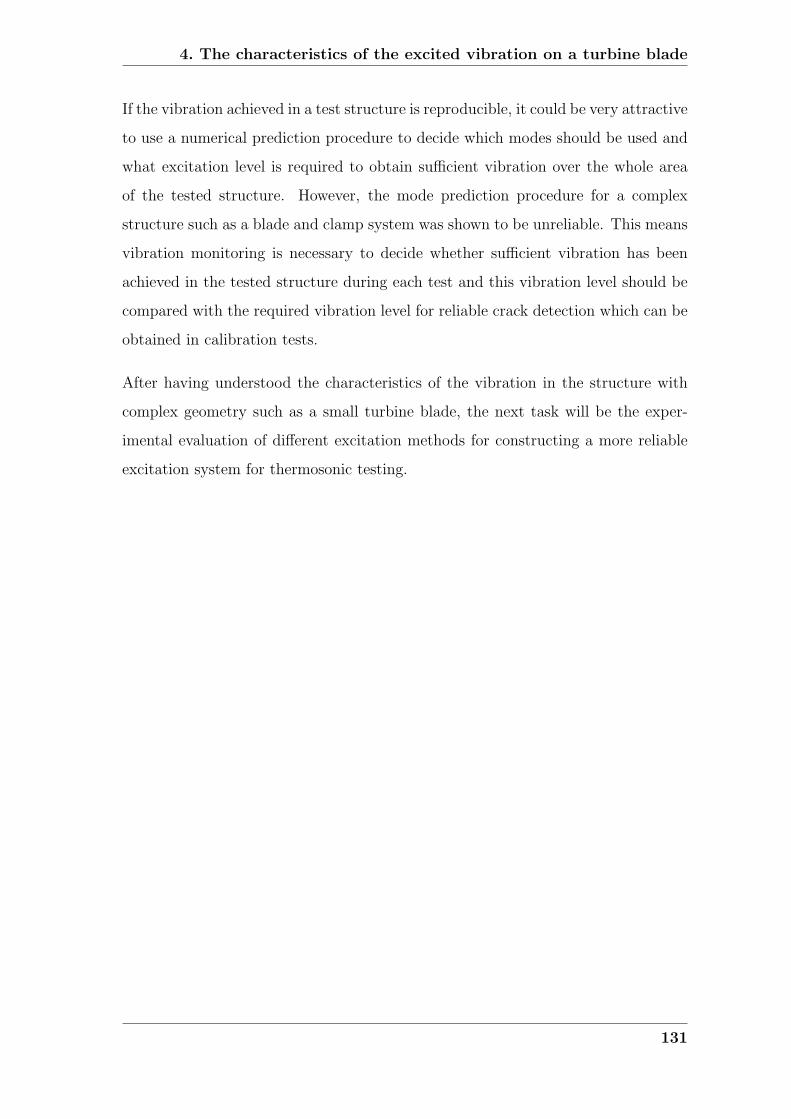
4. The characteristics of the excited vibration on a turbine blade
If the vibration achieved in a test structure is reproducible, it could be very attractive
to use a numerical prediction procedure to decide which modes should be used and
what excitation level is required to obtain sufficient vibration over the whole area
of the tested structure. However, the mode prediction procedure for a complex
structure such as a blade and clamp system was shown to be unreliable. This means
vibration monitoring is necessary to decide whether sufficient vibration has been
achieved in the tested structure during each test and this vibration level should be
compared with the required vibration level for reliable crack detection which can be
obtained in calibration tests.
After having understood the characteristics of the vibration in the structure with
complex geometry such as a small turbine blade, the next task will be the exper-
imental evaluation of different excitation methods for constructing a more reliable
excitation system for thermosonic testing.
131

4. The characteristics of the excited vibration on a turbine blade
IR Camera
Ultrasonic Horn
Blade
Clamp
Strain Gauge
Figure 4.1: Schematic diagram of proposed thermosonics test setup for turbine blade (not
to scale).
Bolt
Blade
Clamp
Figure 4.2: Schematic of blade securing method by bolts and clamp.
132

4. The characteristics of the excited vibration on a turbine blade
SOLARTRON
Frequency Response Analyzer
Power Amplifier
PC
Laser Vibrometer
Velocity
PZT Disc
Clamp
Blade
Laser point
Figure 4.3: Test setup.
35 37 39 41 43 450
0.5
1
1.5
2
2.5
3
Frequency(kHz)
Vel
ocity
(mm
/s)
5 Nm10 Nm15 Nm
Peak 1
Figure 4.4: Measured out-of-plane velocity response at the middle of the blade under
different clamping torque conditions.
133

4. The characteristics of the excited vibration on a turbine blade
35 35.5 36 36.5 370
0.5
1
1.5
2
2.5
3
Frequency(kHz)
Velo
city
(mm
/s)
5 Nm10 Nm
15 Nm
Figure 4.5: Zoomed view of the velocity response around Peak 1 indicated in Figure 4.4.
35000
35200
35400
35600
35800
36000
36200
36400
0 2 4 6 8 10 12 14 16 18Torque(Nm)
Freq
uenc
y(H
z)
Blade-Peak 1Clamp-Peak1
Figure 4.6: Resonance frequency of blade and clamp at the highest peak in Figure 4.5 as
a function of the clamping torque.
134

4. The characteristics of the excited vibration on a turbine blade
A
B
F1F3
Figure 4.7: 3D FEM model of clamp and blade.The manufacturing is controlled so that this has to be within 20deg of axis 1 in any direction. This is the only paramter that they control.The orientation of the other two crystallographic orientations (110 and 111) is monitored but not controlled. I have tried to indicate the orientations on the diagram but I'm not sure how clear it is.
1
3
2
Figure 4.8: Coordinate system for material properties of turbine blade
135

4. The characteristics of the excited vibration on a turbine blade
0
0.2
0.4
0.6
0.8
1
1.2
30 32 34 36 38 40 42 44 46 48 50
Frequency(kHz)
Stra
in( με/
N)
B(ε13)
A(ε22)
31.8 kHz
37.9 kHz
45.4 kHz
Figure 4.9: Strain as a function of frequency at two positions A and B on the blade
shown in Figure 4.7 with 1N point load F1.
39.8 kHz 40.2 kHz 41.7 kHz
44.4 kHz45.4 kHz 47.5 kHz
(a) 31.8 kHz (b) 37.9 kHz (c) 45.4 kHz
Figure 4.10: Blade and clamp system mode shapes at the system resonsnces shown in
Figure 4.9: (a) 31.8 kHz (b) 37.9 kHz (c) 45.4 kHz
136
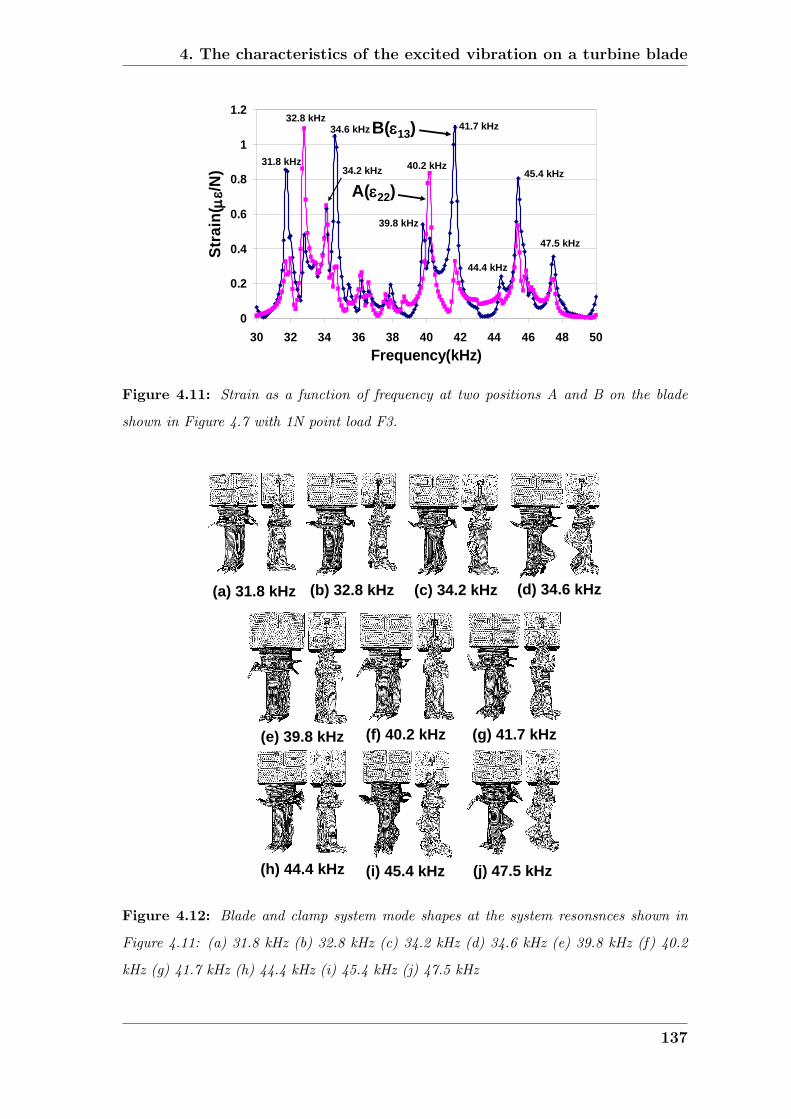
4. The characteristics of the excited vibration on a turbine blade
0
0.2
0.4
0.6
0.8
1
1.2
30 32 34 36 38 40 42 44 46 48 50Frequency(kHz)
Stra
in( με/
N)
B(ε13)
A(ε22)
39.8 kHz
41.7 kHz
40.2 kHz45.4 kHz
44.4 kHz
47.5 kHz
31.8 kHz
32.8 kHz34.6 kHz
34.2 kHz
Figure 4.11: Strain as a function of frequency at two positions A and B on the blade
shown in Figure 4.7 with 1N point load F3.
(e) 39.8 kHz (f) 40.2 kHz (g) 41.7 kHz
(h) 44.4 kHz (i) 45.4 kHz (j) 47.5 kHz
(a) 31.8 kHz (b) 32.8 kHz (c) 34.2 kHz (d) 34.6 kHz
Figure 4.12: Blade and clamp system mode shapes at the system resonsnces shown in
Figure 4.11: (a) 31.8 kHz (b) 32.8 kHz (c) 34.2 kHz (d) 34.6 kHz (e) 39.8 kHz (f) 40.2
kHz (g) 41.7 kHz (h) 44.4 kHz (i) 45.4 kHz (j) 47.5 kHz
137

4. The characteristics of the excited vibration on a turbine blade
0
0.02
0.04
0.06
0.08
0.1
0.12
30 32 34 36 38 40 42 44 46 48 50Frequency(kHz)
Stra
in E
nerg
y D
ensi
ty (J
/m3 /N
)
B
A
39.8 kHz
41.7 kHz
40.2 kHz 45.4 kHz
44.4 kHz47.5 kHz
31.8 kHz
34.6 kHz
34.2 kHz32.8 kHz
Figure 4.13: Strain energy density as a function of frequency at two positions A and B
on the blade with 1N point load F3.
39.8 kHz
41.7 kHz
Front Back
Figure 4.14: Mode Coverage Map; Regions of blade where different modes give largest
strain energy density. 2 mode case: 39.8 kHz (gray) + 41.7 kHz (black).
138
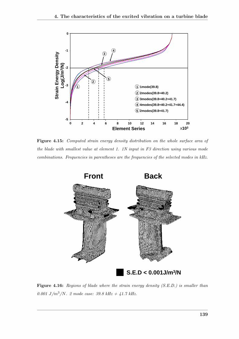
4. The characteristics of the excited vibration on a turbine blade
-1
-2
-3
-4
-5
0
3 3modes(39.8+40.2+41.7)
4 4modes(39.8+40.2+41.7+44.4)
5 2modes(39.8+41.7)
1 1mode(39.8)
2 2modes(39.8+40.2)
12
34
5
0 2 4 6 10 12 14
Element Series8 16 18 20
x103
Stra
in E
nerg
y D
ensi
ty
Log(
J/m
3 /N)
Figure 4.15: Computed strain energy density distribution on the whole surface area of
the blade with smallest value at element 1. 1N input in F3 direction using various mode
combinations. Frequencies in parentheses are the frequencies of the selected modes in kHz.
39.8 kHz
S.E.D < 0.001J/m3/N
Front Back
Figure 4.16: Regions of blade where the strain energy density (S.E.D.) is smaller than
0.001 J/m3/N . 2 mode case: 39.8 kHz + 41.7 kHz.
139

4. The characteristics of the excited vibration on a turbine blade
Α(ε33)
Β(ε33)
Strain Gauge Position
1
23
Figure 4.17: Strain monitoring positions on clamp obtained from 3D FEM results.
00.10.20.30.40.50.60.70.80.9
1
30 32 34 36 38 40 42 44 46 48 50
Frequency(kHz)
Stra
in( με/
N)
Α(ε33)
Β(ε33)
Figure 4.18: Strain as a function of frequency at two positions A and B on the clamp
shown in Figure 4.17 with 1N point load F3.
140

4. The characteristics of the excited vibration on a turbine blade
Table 4.1: Comparison of the detectability of the blade modes shown in Figure 4.13 at
two different positions A and B on the clamp shown in Figure 4.17. (∨: clearly detectable,
s: small peak, vs: very small peak)
Blade mode frequency(kHz) Position A Position B
31.8 vs ∨
32.8 vs ∨
34.2 s ∨
34.6 s ∨
39.8 ∨ ∨
40.2 ∨ ∨
41.7 ∨ s
44.4 ∨ s
45.4 ∨ vs
47.5 ∨ vs
141

4. The characteristics of the excited vibration on a turbine blade
1.00E-06
1.00E-05
1.00E-04
1.00E-03
1.00E-02
1.00E-01
1.00E+00
1.00E+01
0 4000 8000 12000 16000 20000
Element Series
Stra
in E
nerg
y D
ensi
ty (J
/m3 /N
) 2modes(39.8+41.7)
0.001
0.01
0.1
1
10
0 5000 10000 15000 20000
Element Series
Stra
in ε
11( με/Ν
)
(b)
(a)
Figure 4.19: Distribution of strain energy density and strain (ε11) on the whole surface
area of the blade. 1N input in F3 direction using two modes of 39.8 and 41.7 kHz: (a)
Strain energy density distribution on the whole surface area of the blade with smallest value
at element 1 (b) Strain (ε11) of the corresponding elements shown in (a).
142

4. The characteristics of the excited vibration on a turbine blade
0.001
0.01
0.1
1
4390 4410 4430 4450 4470 4490 4510Element Series
Stra
in( με/Ν
)
E11E22E33E12E13E23
SED = 0.01 - 0.0102J/m3/N
Figure 4.20: Six strain components of the elements with strain energy density 0.01 -
0.0102 J/m3. 1N input in F3 direction using two modes (39.8 and 41.7 kHz).
143
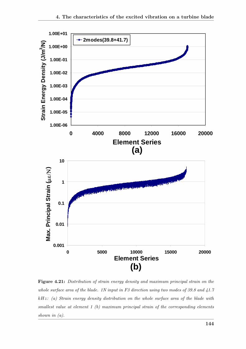
4. The characteristics of the excited vibration on a turbine blade
1.00E-06
1.00E-05
1.00E-04
1.00E-03
1.00E-02
1.00E-01
1.00E+00
1.00E+01
0 4000 8000 12000 16000 20000Element Series
Stra
in E
nerg
y D
ensi
ty (J
/m3 /N
) 2modes(39.8+41.7)
0.001
0.01
0.1
1
10
0 5000 10000 15000 20000Element Series
Max
. Prin
cipa
l Str
ain
( με/Ν
)
(b)
(a)
Figure 4.21: Distribution of strain energy density and maximum principal strain on the
whole surface area of the blade. 1N input in F3 direction using two modes of 39.8 and 41.7
kHz: (a) Strain energy density distribution on the whole surface area of the blade with
smallest value at element 1 (b) maximum principal strain of the corresponding elements
shown in (a).
144

4. The characteristics of the excited vibration on a turbine blade
0
0.2
0.4
0.6
0.8
1
1.2
20 25 30 35 40 45 50Frequency(kHz)
Velo
city
(mm
/s)
EXPERIMENT3D FEM
0
1
2
3
4
5
6
20 25 30 35 40 45 50Frequency(kHz)
Velo
city
(mm
/s)
EXPERIMENT3D FEM
(a)
(b)
1
2
3
5
4
1
4
3
1
2
3
4
2
3
4 5
5
2
ii
ExperimentFEM
Peaks are corresponding to mode i
Figure 4.22: Out of plane velocity responses at the clamp shown in Figure 4.23(a): (a)
responses at the center of the top surface; (b) responses at the center of the side surface.
145

4. The characteristics of the excited vibration on a turbine blade
Top
Side
Blade
Top
Side
(a) (b)
Figure 4.23: Surfaces used for mode shape measurement: (a)clamp; (b)clamp and blade
system.
Experiment
SideTop
25.0 kHz
27.8 kHz
47.3 kHz
41.6 kHz
43.2 kHz
3D FEMSideTop
25.8 kHz
28.5 kHz
48.4 kHz
42.4 kHz
45.0 kHz
FRF for mode identification
1
2
4
3
5
1
2
3
4
5
Figure 4.24: Comparison of measured mode shapes and analytical mode shapes calculated
by 3D FEM.
146

4. The characteristics of the excited vibration on a turbine blade
0
0.5
1
1.5
2
2.5
3
30 35 40 45 50Frequency(kHz)
Velo
city
(mm
/s)
EXPERIMENT3D FEM
Position B
(b)
(a)
0
0.2
0.4
0.6
0.8
1
1.2
1.4
1.6
30 35 40 45 50Frequency(kHz)
Velo
city
(mm
/s)
EXPERIMENT3D FEM
Position A
1
23
4
Figure 4.25: Out of plane velocity responses at positions A and B shown in 4.7: (a)
Position A (b) Position B
147

4. The characteristics of the excited vibration on a turbine blade
Including the diagragm of the selected surface
1 2 3 4 5 6 7 8 9 101
2
3
4
5
0.2
0.4
0.6
1.0
0.8
5 experiments by 10 analysis
Expe
rimen
t
Analysis
2 4 6 8 10 12 14 16 18 201234
0.2
0.4
0.6
4 experiments by 21 analysis
Expe
rimen
t
Analysis
(a)
(b)
Figure 4.26: Presentation of MAC: (a) clamp only model; (b) clamp and blade system
model.
148

Chapter 5
Multiple mode excitation system
for reliable crack detection
5.1 Introduction
Several studies have shown that a rich spectrum of vibration greatly improves the
temperature rise in thermosonic testing [2, 43, 90]. Morbidini et al. [14] have shown
that there is a quantitative relationship between the temperature rise, the damp-
ing, vibration amplitude and frequency characteristics of the vibration. It was
also discussed in Chapter 2 and Chapter 3 that multiple mode excitation is re-
quired to obtain enough strain over the whole structure for reliable thermosonic
testing [40,41,91].
Therefore, the influence of the clamping method and the excitation signal that is
input to the horn on the vibration characteristics are studied experimentally and
presented in this chapter. A reliable excitation method for the structures with
complex geometry such as turbine blades is essential if the test is to be used in
industries. The experimental study in this chapter was conducted on a small turbine
blade that is one of the challenging structures for reliable inspection. A fast narrow
band sweep test with a general purpose amplifier and stud coupling is presented
as an excitation method. This method can be applied to different types of turbine
149
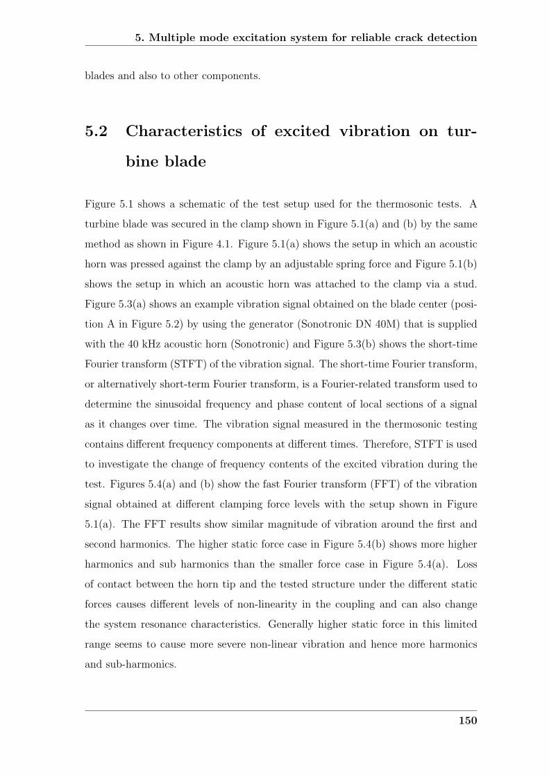
5. Multiple mode excitation system for reliable crack detection
blades and also to other components.
5.2 Characteristics of excited vibration on tur-
bine blade
Figure 5.1 shows a schematic of the test setup used for the thermosonic tests. A
turbine blade was secured in the clamp shown in Figure 5.1(a) and (b) by the same
method as shown in Figure 4.1. Figure 5.1(a) shows the setup in which an acoustic
horn was pressed against the clamp by an adjustable spring force and Figure 5.1(b)
shows the setup in which an acoustic horn was attached to the clamp via a stud.
Figure 5.3(a) shows an example vibration signal obtained on the blade center (posi-
tion A in Figure 5.2) by using the generator (Sonotronic DN 40M) that is supplied
with the 40 kHz acoustic horn (Sonotronic) and Figure 5.3(b) shows the short-time
Fourier transform (STFT) of the vibration signal. The short-time Fourier transform,
or alternatively short-term Fourier transform, is a Fourier-related transform used to
determine the sinusoidal frequency and phase content of local sections of a signal
as it changes over time. The vibration signal measured in the thermosonic testing
contains different frequency components at different times. Therefore, STFT is used
to investigate the change of frequency contents of the excited vibration during the
test. Figures 5.4(a) and (b) show the fast Fourier transform (FFT) of the vibration
signal obtained at different clamping force levels with the setup shown in Figure
5.1(a). The FFT results show similar magnitude of vibration around the first and
second harmonics. The higher static force case in Figure 5.4(b) shows more higher
harmonics and sub harmonics than the smaller force case in Figure 5.4(a). Loss
of contact between the horn tip and the tested structure under the different static
forces causes different levels of non-linearity in the coupling and can also change
the system resonance characteristics. Generally higher static force in this limited
range seems to cause more severe non-linear vibration and hence more harmonics
and sub-harmonics.
150

5. Multiple mode excitation system for reliable crack detection
5.3 Effect of stud coupling on blade vibration
As presented in the previous section, the acoustic horn can be attached to the clamp
via a stud instead of using spring force to couple the horn to the clamp as shown
in Figure 5.1(b). Experiments were conducted in order to investigate the effect of
the different coupling methods on the vibration in the blade. A controllable general
purpose power amplifier (AG 1012) supplied by T&C Power Conversion was used
for supplying power to the acoustic horn. Two different test modes can be used by
varying the input signal from a function generator (Agilent 33220A) to the amplifier;
a single frequency sine wave and a fast frequency sweep that will be used for tests in
a later section. The single frequency sine wave was used for tests presented in this
section. Figure 5.5 (a) and Figure 5.6(a) show the vibration obtained during single
frequency excitation tuned to the system resonance at 43.8 kHz when the acoustic
horn was coupled to the clamp by using a stud. Figures 5.5(b) and 5.6(b) show the
STFT of the vibration in Figure 5.5(a) and Figure 5.6(a) respectively. Generally
stud coupling generates single frequency vibration at low power input level as shown
in Figure 5.5(b) but many high harmonics and sub harmonics at higher power setting
(200W) as shown in Figure 5.6(b). This is probably caused by clapping of the horn
tip against the clamp. Figure 5.7 shows the peak vibration amplitude at blade
center obtained during single frequency excitation at system resonance of 43.8 kHz
for a stud coupling case and 40.2 kHz for a spring force coupling case as a function
of power setting in the amplifier. The stud coupling case shows significantly higher
peak velocity than the spring case. Generally as the power setting increases the peak
velocity increases until a certain value of power setting and then the peak velocity
was saturated.
5.4 The effect of power amplifier on the vibration
If the horn is excited by a pure sine wave at the horn resonance frequency via a high
fidelity power amplifier, the dominant frequencies in the response are the input fre-
151
5. Multiple mode excitation system for reliable crack detection
quency and its harmonics and sub-harmonics that are generated by the non-linearity
of the coupling. Figure 5.8 shows the rich FFT of the vibration, obtained by using
the horn generator that is supplied with an acoustic horn, around the fundamental
and the first harmonic of the excitation frequency of the acoustic horn. The results
of multiple tests were shown in Figure 5.8 because one typical characteristic of a
thermosonic test is the lack of repeatability in the amplitude and the frequency
characteristic of the vibration. These results show interesting results: several modes
within a 4 kHz bandwidth around the fundamental and the first harmonic are ex-
cited, though at very different amplitude.
To find the cause of the broad band excitation in Figure 5.8, the effect of the amplifier
characteristic on the vibration was investigated. Figure 5.9 shows the STFT and
FFT of the vibration obtained by using the horn generator (Sonotronic DN 40M) and
a general purpose power amplifier (AG 1012). When the general purpose amplifier
was used for the test, the horn was excited at a system resonance of 40.2 kHz
controlled by a function generator input to the amplifier and 500W power setting
in the amplifier was used for the test. Figure 5.9 shows the typical characteristics
that were found in many test results with both amplifiers. Figure 5.9 shows that
the fundamental and the first harmonic of the excitation frequency are dominant
with both amplifiers and there are several small higher order harmonic components.
Figure 5.9(a3) also shows that the first harmonic component is typically larger than
the fundamental component with the horn generator.
Figure 5.10 show the results obtained from a test with a horn generator shown in
Figure 5.9(a) in more detail around the fundamental frequency together with the
corresponding input voltage characteristics. STFTs of the velocity and the input
voltage are shown respectively in Figure 5.10 (a2) and (b2). Frequency components
in both figures vary until 200 ms and then become steady but the final frequency
is not 40 kHz which is a nominal excitation frequency of the horn. This frequency
characteristic is also seen in the FFT of the total signal of the velocity and input
voltage shown in Figures 5.10(a3) and (b3). The highest peak is not 40 kHz but
39.85 kHz in both Figures 5.10(a3) and (b3). This seems to be caused by the lowest
152

5. Multiple mode excitation system for reliable crack detection
impedance searching mechanism in the horn generator. Figure 5.10(b2) shows the
characteristics of the hunting mechanism that the hunting starts around 40.5 kHz
which caused a hump around the 40.5 kHz in Figure 5.10(b3). While it is hunting the
lowest impedance frequency, different modes are excited and this results in different
humps in Figure 5.10(a3) in the vibration signal. Away from the final frequency,
the amplitudes are relatively low in the FFT of the total signal as shown in Figure
5.10(a3). This result suggests that a chirp input could be a way of exciting multiple
modes in turn in a more controlled fashion. Figure 5.11 shows the corresponding
results for the general purpose amplifier case of Figure 5.9(b). The horn was excited
at a system resonance of 40.2 kHz controlled by a function generator input to the
amplifier and a 500 W power setting in the amplifier was used for this test. In this
case the vibration is at a single frequency corresponding to the input.
The results in Figure 5.10 and Figure 5.11 show that the input voltage signal affects
the frequency characteristics of the vibration and the broad band response produced
by the horn generator is caused by a lock-in control system in the horn generator that
searches for the main system resonance. This suggests that a controlled sweep test
around the resonances of the system comprising the component and the excitation
system can provide a higher response because the excitation frequency will sweep
through multiple resonances. This can be achieved by employing a chirp input over
a frequency range centered on the system resonance frequency.
5.5 The characteristics of the vibration measured
during sweep test
In order to investigate the characteristics of the vibration produced in sweep tests,
linear frequency sweep tests were conducted by using the sweep input signal from a
function generator (Agilent 33220A) to the amplifier. A controllable general purpose
power amplifier (AG 1012) was used for supplying power to the acoustic horn.
Figures 5.12(a1) and (b1) show the vibration obtained from a linear sweep test with
153

5. Multiple mode excitation system for reliable crack detection
sweep frequency range from 35 kHz to 45 kHz and sweep time of 1 sec. Two different
coupling methods, stud and spring force, were used for the tests shown in Figures
5.12(a1) and (b1) respectively. Higher vibration amplitudes are seen at the system
resonances in the frequency range of the sweep in Figures 5.12(a1) and (b1). The
excitation frequency changed linearly from 35 kHz to 45 kHz within the sweep time
of 1 sec. Figures 5.12(a2) and (b2) show the corresponding STFT of the vibration
obtained from the sweep test. This shows that higher amplitudes are seen at simple
multiple of excitation frequency and many harmonics are excited especially in the
stud coupling case. In particular, around the high response frequency of 44 kHz,
many harmonics are excited as shown in Figure 5.12(a2). These harmonic com-
ponents can enhance the thermal image [2]. Figures 5.12 (a3) and (b3) show the
corresponding FFTs of the vibration in Figures 5.12(a1) and (b1) and corresponding
peaks marked by the same numbers can be identified between the vibration in Fig-
ures 5.12(a1) and (b1) and the FFTs in Figures 5.12 (a3) and (b3). These results
show that a controlled sweep test around the resonances of the system compris-
ing the component and the excitation system can provide a higher response as the
excitation frequency sweeps through multiple resonances and multiple modes with
similar amplitude in the frequency range of the sweep are excited during the sweep
test.
Figure 5.13 shows the impedance frequency response measured at the input to the
acoustic horn in two different coupling conditions. There are several minima in
both cases indicating multiple system resonances. The stud coupling case shows
the lowest impedance at around 44 kHz but the spring force case shows the lowest
impedance at around 40 kHz and 42 kHz. Generally the lowest impedance value is
much smaller in the stud coupling case than the spring force case. Different spring
force levels also changed the impedance response and the impedance minimum value.
These results show that the coupling condition can change the system resonance
frequency and the effective power transfer into the tested structure. For example,
the vibration in Figure 5.12(a1) shows very high responses at around the lowest
impedance frequency of 44 kHz in the stud coupling case. At this frequency, the
vibration shows a combination of high frequency components and a discontinuity.
154
5. Multiple mode excitation system for reliable crack detection
This discontinuity is probably due to chattering and slip at the interface between
the clamp and the tip of the acoustic horn under high vibration conditions. The
high vibration levels at the high power transfer condition at the lowest impedance at
around 44 kHz could change the coupling condition and so produce a discontinuity
in the vibration.
Figure 5.12 shows the results obtained from a relatively broad band sweep test with
a 10 kHz band. However, a narrow band sweep test may provide higher responses
around the system resonance frequencies because a longer excitation can be achieved
around the system resonances. Therefore, fast narrow band sweep tests were con-
ducted to investigate the vibration characteristics of the narrow band sweep test.
Figure 5.14 shows test results obtained from a fast narrow band sweep test. A 2
kHz band around the peak resonances of Figures 5.12(a1) and (b1) for the stud and
spring cases respectively was selected for the sweep tests. This result also shows
that larger amplitudes are obtained in the stud coupling case and many harmonics
are excited especially in the stud coupling case around the frequency range between
43 kHz and 44 kHz as shown in Figure 5.14(a2).
Figure 5.15 shows the spectrum of the vibration obtained from the fast narrow band
sweep test shown in Figure 5.14. It will be shown in Chapter 6 that it is possible
to predict the temperature rise obtained at a given crack from a measurement of
the spectrum of vibration at the crack site. This is based on the calculation of
a parameter termed the Heating Index (HI) [3, 14]. Two different time sections
in the STFT shown in Figure 5.15(a) that produce similar high amplitudes in the
Heating Index shown in Figure 5.15(b) were selected to investigate the frequency
characteristics of the vibration. Figure 5.15(c) shows the spectrum at time 1 (the 5th
time section of the STFT) and Figure 5.15(d) shows the spectrum at time 2 (the 21st
time section of the STFT). In each case the vibration consists of the fundamental
frequency and its harmonics, the fundamental frequency being different at the two
instants because of the sweep input. At time 2 the vibration is predominantly at
the fundamental frequency, while at time 1 the harmonics dominate, none of them
reaching the amplitude of the fundamental at time 2. However, the heating index
155
5. Multiple mode excitation system for reliable crack detection
at the two times is similar. This means that both cases give a similar temperature
rise for a crack at the vibration measurement position. However, the multiple mode
excitation obtained at time 1 is much better for achieving sufficient vibration over
the whole surface area of the blade for reliable thermosonic testing when the crack
position is not known.
5.6 Effect of impedance matching on vibration
level
In the previous section, it was seen that the vibration amplitude strongly depends
on the impedance measured at the input to the acoustic horn. In the case of the
acoustic horn used for thermosonics, the impedance of the load can vary due to
changing test configuration, operating frequencies and target structures. In some
cases, an impedance matching circuit can be used to improve the power transfer to
the load side [92]. Therefore, the effect of impedance matching on the vibration was
investigated. Figure 5.16 shows the measured impedance frequency responses with
and without an impedance matching circuit and Figure 5.17 shows the comparison
of the vibration obtained during different sweep tests with different matching con-
ditions shown in Figure 5.16. The results in Figures 5.16 and 5.17 were obtained
under the same test configuration. The acoustic horn was coupled by a spring force
of 380N in both cases in Figure 5.16 and Figure 5.17. As shown in Figure 5.16, there
are several minima in both cases indicating multiple system resonances. Usually,
the source impedance is 50 Ω at the output in high power ultrasonic amplifier and
the load impedance under the spring force coupling condition is around 1000 Ω in
the test configuration as shown in Figure 5.16. Therefore, an impedance matching
circuit that lowers the overall impedance from 1000 Ω to 50 Ω was applied between
the amplifier output and the input to the acoustic horn in this case. The matching
circuit is a simple transformer with an appropriate transformer ratio to match the
impedance in this study. The matching case in Figure 5.17(b) shows about 2.5 times
higher peak responses than the case without matching in Figure 5.17(a). This result
156
5. Multiple mode excitation system for reliable crack detection
shows that impedance matching can improve the power transfer to the load side and
increase the vibration level in the tested structure.
Figure 5.18 shows spectrum of the vibration obtained from a sweep test with spring
force coupling and impedance matching shown in Figure 5.17. Two different time
sections in the STFT shown in Figure 5.18(a) that show relatively higher amplitude
in the Heating Index shown in Figure 5.18(b) were selected to investigate the fre-
quency characteristics of the vibration. Figure 5.18(c) shows the spectrum at time
1(the 15th time section of the STFT) and Figure 5.18(d) shows the spectrum at
time 2 (the 46th time section of the STFT). The fundamental frequency is different
at the two instants because of the sweep input. At time 2 the vibration is pre-
dominantly at the fundamental frequency (58.1 kHz), while the spectrum at time 1
shows typical chaotic vibration characteristics. However, the heating index at the
two times is similar. The spectrum at time 1 shows that the peaks are seen at the
excitation frequency (45.9 kHz) and simple multiple of the excitation frequency but
also multiple modes are excited as side bands with different magnitudes around the
excitation frequency (45.9 kHz) and the harmonics of the excitation frequency. None
of the frequency components at time 1 reach the amplitude of the fundamental at
time 2 and the highest peak is at 95.2 kHz near the first harmonic (91.8 kHz) of
the excitation frequency (45.9 kHz). From the reliable excitation point of view, the
chaotic vibration shown in Figure 5.18(c) is much better than the single frequency
dominant vibration shown in Figure 5.18(d) because this rich spectrum of vibration
reduces the likelihood of region where the vibration amplitude is very low occurring,
so improving the reliability of the test.
5.7 Review of Chapter
This chapter presented the influences of the coupling method and the excitation
signal that is input to the horn on the excited vibration.
In some cases it is possible to secure the component to be tested in a clamp and to
attach the horn to the clamp via a stud. The stud coupling generally generates higher
157

5. Multiple mode excitation system for reliable crack detection
amplitude vibrations than spring force coupling. The vibration shows very high
responses at around the lowest impedance frequency especially in the stud coupling
case. In the spring force coupling case which shows relatively high impedance over
a wide frequency range, impedance matching can improve the power transfer to the
load side and produce higher vibration levels in the tested structure.
A higher response can be obtained if the excitation frequency coincides with the
resonance of the system comprising the component and the excitation system. This
has been achieved by employing a chirp input over a frequency range centered on the
system resonance frequency. Significant vibration amplitudes are then seen at the
system resonances which coincide with simple multiples of the excitation frequency
in the frequency range of the chirp, and at some frequencies multiple modes around
the excitation frequency and the harmonics of the excitation frequency are also
excited; this rich spectrum of vibration reduces the likelihood of region where the
vibration amplitude is very low occurring, so improving the reliability of the test.
Thermosonic testing is often done using the generator that is supplied with an
acoustic horn. While the input frequency is nominally at the resonance frequency
of the horn, the amplifier hunts for the true resonance so it is not a fixed frequency
device. However, a fast narrow band sweep test using a general purpose amplifier
offers the possibility of exciting many modes with similar amplitude in turn around
the horn resonance and this does not require a tuning procedure. As a result of
the investigation, a fast narrow band sweep test with a general purpose amplifier
and stud coupling is proposed as an excitation method for thermosonic testing.
This method can be applied to different types of turbine blades and also to other
components.
One typical characteristic of a thermosonic test using non-linear vibration is the lack
of repeatability in the amplitude and the frequency characteristics of the vibration.
This means vibration monitoring is necessary to decide whether sufficient vibration
has been achieved in the tested structure. The vibration level should be compared
with the required vibration level for reliable crack detection which can be obtained in
calibration tests. This calibration procedure will be explained in Chapter 6 and the
158

5. Multiple mode excitation system for reliable crack detection
performance of different sensors for vibration monitoring will also be investigated
and compared.
159

5. Multiple mode excitation system for reliable crack detection
(b)
Clamp
Blade
Stud
Acoustic Horn
Foam Material
(a)
Blade
Clamp
Acoustic Horn
Post
d
Spring
Bolt
Figure 5.1: Schematic of test setup used for the thermosonic tests, (a) spring force
coupling; (b) stud coupling.
160

5. Multiple mode excitation system for reliable crack detection
AB
Measurement Position
Figure 5.2: Vibration measurement position.
(b)
0 500 10000
50
100
150
200
250
300
Freq
uenc
y(kH
z)
time(ms)
-20
0
20
40
(a)
-200 0 200 400 600 800 1000-400-300-200-1000
100200300400500
Velo
city
(mm
/s)
time(ms)
dB
Figure 5.3: Typical vibration signal and STFT of the vibration signal measured on the
blade center. (a) Vibration signal; (b) STFT of the vibration.
161

5. Multiple mode excitation system for reliable crack detection
(a) (b)
Figure 5.4: Spectrum of the vibration signal measured on the blade center at two different
static force levels. (a) spectrum at F=180N; (b) spectrum at F=380 N.
162

5. Multiple mode excitation system for reliable crack detection
Low power : single
(a) (b)
0 500 1000-1500
-1000
-500
0
500
1000
1500Ve
loci
ty(m
m/s
)
time(ms)0 500 10000
50
100
150
200
250
Freq
uenc
y(kH
z)
time(ms)-20
0
20
40
dB
Figure 5.5: Vibration obtained during single frequency excitation under the stud coupling
condition; power setting is 5 W, (a) Vibration signal; (b) STFT of the vibration signal on
the blade center.
0 200 400 600 800 1000-1500
-1000
-500
0
500
1000
1500
Velo
city
(mm
/s)
time(ms)0 500 10000
50
100
150
200
250
Freq
uenc
y(kH
z)
time(ms)-20
0
20
40
60
dB
(a) (b)
Figure 5.6: Vibration obtained during single frequency excitation under the stud coupling
condition; power setting is 200 W, (a) Vibration signal; (b) STFT of the vibration signal
on the blade center.
163

5. Multiple mode excitation system for reliable crack detection
(F=330N)
0
200
400
600
800
1000
1200
1400
1600
0 100 200 300 400 500 600Amplifier Power Setting(W)
Peak
Am
plitu
de(m
m/s
) Stud
Spring
Figure 5.7: Peak vibration amplitude at blade center vs power setting for single frequency
excitation at system resonance.
(a) (b)
Figure 5.8: Spectrum of the vibration signal measured on the blade center at the static
force level of 330 N. (a) around 40 kHz (fundamental); (b) around 80 kHz (the first har-
monic).
164

5. Multiple mode excitation system for reliable crack detection
0 50 100 150 200 250 3000
20
40
60
80
100
120
Frequency(kHz)
Am
plitu
de-V
eloc
ity(m
m/s
)
time(ms)0 200 400 600 800 1000-800
-600
-400
-200
0
200
400
600
800
Velo
city
(mm
/s)
Horn Generator(a1)
(a2)
(a3)
0 200 400 600 800 1000-1200-1000-800-600-400-200
0200400600800
Velo
city
(mm
/s)
time(ms)
(b1)
(a2)
General purpose amplifier
Am
plitu
de-V
eloc
ity(m
m/s
)
0 50 100 150 200 250 3000
50
100
150
200
250
300
Frequency(kHz)
(b3)
0 200 400 600 800 10000
50
100
150
200
250
300
Freq
uenc
y(kH
z)
time(ms)-30
-20
-10
0
10
20
30
dB
0 200 400 600 800 10000
50
100
150
200
250
300
Freq
uenc
y(kH
z)
time(ms)-30
-20
-10
0
10
20
30
40
dB
(b2)(a2)
Figure 5.9: STFT and FFT of the vibration signal measured on the blade center during
tests with different input method (F=330 N). (a1) Velocity, (a2) STFT of the velocity,
(a3) Spectrum of the velocity, (b1) Velocity, (b2) STFT of the velocity, (b3) Spectrum of
the velocity
165

5. Multiple mode excitation system for reliable crack detection
time(ms)0 200 400 600 800 1000-800
-600
-400
-200
0
200
400
600
800
Velo
city
(mm
/s)
time(ms)0 200 400 600 800 100039
39.2
39.4
39.6
39.8
40
40.2
40.4
40.6
40.8
41
Freq
uenc
y(kH
z)
0
5
10
15
20
25
30
35
40
45
39 39.5 40 40.5 410
5
10
15
20
25
30
35
40
Frequency(kHz)
Am
plitu
de-V
eloc
ity(m
m/s
)
0 200 400 600 800 1000-1500
-1000
-500
0
500
1000
1500
Inpu
t Vol
tage
(V)
time(ms)
time(ms)
50msGENERATORVelocity on blade Input Voltage
(a1) (b1)
(a2)
(a3)
0 200 400 600 800 100039
39.2
39.4
39.6
39.8
40
40.2
40.4
40.6
40.8
41
Freq
uenc
y(kH
z)
0
10
20
30
40
50(b2)
39 39.5 40 40.5 410
50
100
150
200
250
300
350
400
450
Frequency(kHz)
Am
plitu
de-In
put V
olta
ge(V
)
(b3)
dB dB
Figure 5.10: The characteristics of the vibration and the input voltage signal obtained
from a test with a horn generator:(a1) Velocity, (a2) STFT of velocity around 40 kHz, (a3)
Spectrum of the velocity around 40 kHz, (b1) Input voltage, (b2) STFT of input voltage
around 40 kHz, (b3) Spectrum of the input voltage around 40 kHz
166
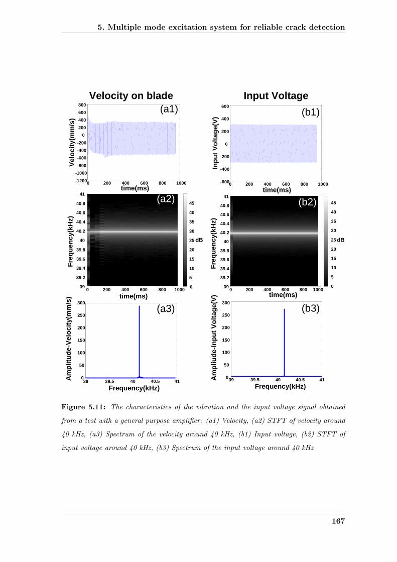
5. Multiple mode excitation system for reliable crack detection
50msAG
0 200 400 600 800 1000-1200-1000-800-600-400-200
0200400600800
Velo
city
(mm
/s)
time(ms)
0 200 400 600 800 100039
39.2
39.4
39.6
39.8
40
40.2
40.4
40.6
40.8
41
Freq
uenc
y(kH
z)
time(ms)0
5
10
15
20
25
30
35
40
45
39 39.5 40 40.5 410
50
100
150
200
250
300
Frequency(kHz)
Am
plitu
de-V
eloc
ity(m
m/s
)
0 200 400 600 800 1000-600
-400
-200
0
200
400
600
Inpu
t Vol
tage
(V)
time(ms)
0 200 400 600 800 100039
39.2
39.4
39.6
39.8
40
40.2
40.4
40.6
40.8
41
Freq
uenc
y(kH
z)
time(ms)0
5
10
15
20
25
30
35
40
45
39 39.5 40 40.5 410
50
100
150
200
250
300
Frequency(kHz)
Am
pliu
de-In
put V
olta
ge(V
)
(a1) (b1)
(a2)
(a3)
(b2)
(b3)
Velocity on blade Input Voltage
dB dB
40178 Hz / 500W
Figure 5.11: The characteristics of the vibration and the input voltage signal obtained
from a test with a general purpose amplifier: (a1) Velocity, (a2) STFT of velocity around
40 kHz, (a3) Spectrum of the velocity around 40 kHz, (b1) Input voltage, (b2) STFT of
input voltage around 40 kHz, (b3) Spectrum of the input voltage around 40 kHz
167

5. Multiple mode excitation system for reliable crack detection
0 200 400 600 800 1000-2000
-1500
-1000
-500
0
500
1000
1500
2000
Velo
city
(mm
/s)
time(ms)
Frequency (kHz)35 40 45
1 32
4
5
(a1)
0 200 400 600 800 1000-2000
-1500
-1000
-500
0
500
1000
1500
2000
Velo
city
(mm
/s)
time(ms)
Frequency (kHz)35 40 45
2 31
(b1)
35 36 37 38 39 40 41 42 43 44 450
1
2
3
4
5
6
7
Frequency (kHz)
|V(f)
|
1 3
2
4
5
(a3)
35 36 37 38 39 40 41 42 43 44 450
1
2
3
4
5
6
7
Frequency (kHz)
|V(f)
| 1
2
3
(b3)
dB
dB
0 200 400 600 800 10000
50
100
150
200
250
Freq
uenc
y(kH
z)
time(ms)
-60
-40
-20
0
20
40
60(a2)
-60
-40
-20
0 200 400 600 800 10000
50
100
150
200
250
Freq
uenc
y(kH
z)
time(ms)
0
20
40(b2)
Figure 5.12: Vibration, corresponding STFT and FFT of the vibration obtained from a
sweep test: (a1), (a2), (a3) Stud coupling; (b1), (b2), (b3) Spring force coupling.
Stud
Spring
Figure 5.13: Impedance frequency responses measured at the input to the acoustic horn
with spring and stud coupling.
168
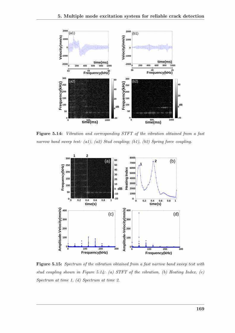
5. Multiple mode excitation system for reliable crack detection
dB
-2000
-1000
0
1000
2000
Velo
city
(mm
/s)
time(ms)
Frequency(kHz)43 44 45
0 200 400 600 800 1000
(a1)
300
0 500 10000
50
100
150
200
250
Freq
uenc
y(kH
z)
time(ms)-20
0
20
40
60(a2)
0 200 400 600 800 1000-2000
-1000
0
1000
2000
Velo
city
(mm
/s)
time(ms)
39 40 41Frequency(kHz)
(b1)
0 500 10000
50
100
150
200
250
300
Freq
uenc
y(kH
z)time(ms)
-20
0
20
40
dB
(b2)
Figure 5.14: Vibration and corresponding STFT of the vibration obtained from a fast
narrow band sweep test: (a1), (a2) Stud coupling; (b1), (b2) Spring force coupling.
20ms 5 21
0 0.2 0.4 0.6 0.8 10
50
100
150
200
250
300
Freq
uenc
y(kH
z)
time(s)-20
-10
0
10
20
30
40
50
601 2
dB
(a)
0 100 200 3000
100
200
300
400
Frequency(kHz)
Am
plitu
de-V
eloc
ity(m
m/s
)
(c)
0 100 200 3000
100
200
300
400
Frequency(kHz)
Am
plitu
de-V
eloc
ity(m
m/s
)
(d)
0 0.2 0.4 0.6 0.8 10
1000
2000
3000
4000
5000
6000
7000
8000
time(s)
Hea
ting
Inde
x
12 (b)
Figure 5.15: Spectrum of the vibration obtained from a fast narrow band sweep test with
stud coupling shown in Figure 5.14: (a) STFT of the vibration, (b) Heating Index, (c)
Spectrum at time 1, (d) Spectrum at time 2.
169

5. Multiple mode excitation system for reliable crack detection
1
10
100
1000
10000
100000
40000 45000 50000 55000 60000
Frequency(Hz)
Impe
danc
e(Ω
)
Matching
Without Matching
Figure 5.16: Impedance frequency responses measured at the input to the acoustic horn
with and without impedance matching circuit.
0 100 200 300 400 500 600 700 800 900 1000
time(ms)-600
-400
-200
0
200
400
600
Velo
city
(mm
/s)
0 100 200 300 400 500 600 700 800 900 1000time(ms)
-800
-600
-400
-200
0
200
400
600
Velo
city
(mm
/s)
(a) (b)Frequency(kHz)
40 6045 5550Frequency(kHz)
40 6045 5550
Figure 5.17: Vibration measured during a sweep test with spring force coupling. (a)
without impedance matching; (b)with impedance matching.
170

5. Multiple mode excitation system for reliable crack detection
(a)
0 0.2 0.4 0.6 0.8 10
50
100
150
200
250
300
Freq
uenc
y(kH
z)
time(s)-20
-10
0
10
20
30
40(a)
dB
0 0.2 0.4 0.6 0.8 10
500
1000
1500
2000
2500
3000
3500
4000
time(s)
Hea
ting
Inde
x
(b)
(d)
0 50 100 150 200 250 3000
102030405060708090
100
Frequency(kHz)
Am
plitu
de-V
eloc
ity(m
m/s
)
(d)
0 50 100 150 200 250 300Frequency(kHz)
Am
plitu
de-V
eloc
ity(m
m/s
)
0102030405060708090
100(c)
12
95.2kHz
91.8kHz45.9kHz
58.1kHz
116.1kHz
87.4kHz
Figure 5.18: Spectrum of the vibration obtained from a sweep test with spring force
coupling and impedance matching shown in Figure 5.17(b): (a) STFT of the vibration, (b)
Heating Index, (c) Spectrum at time 1, (d) Spectrum at time 2.
171

Chapter 6
Vibration monitoring for reliable
thermosonic testing
6.1 Introduction
Prediction of mode shapes is very attractive to decide which mode should be used
and what excitation level is required to obtain sufficient vibration over the whole
area of the tested structure. However, the mode prediction procedure for a complex
structure such as a blade and clamp system is not reliable as presented in Chapter
4. One typical characteristic of a thermosonic test is the lack of repeatability in the
amplitude and the frequency characteristic of the vibration. This means vibration
monitoring is necessary to decide whether sufficient vibration is achieved in tested
structures during each test and the vibration level should be compared with the
required vibration level for reliable crack detection which can be obtained in cali-
bration tests. Therefore, a calibration test procedure is required to find the required
vibration level for the reliable detection of the target defects.
Thermosonics uses vibrational energy to detect defects in structures and this vibra-
tional energy is converted into heat at the defect. The surface temperature rise is
detected by a thermal imaging camera. There are several parameters that influence
the temperature rise at the defect, the most well known of which are the cyclic
172

6. Vibration monitoring for reliable thermosonic testing
strain, frequency of vibration, damping characteristic, crack morphology and ther-
mal properties of the structure [70,75–77]. If other parameters remain constant, the
temperature rise ∆T can be expressed approximately as [3, 14,15]:
∆T ∝ ηrε2f (6.1)
where ε is the amplitude of cyclic strain, f is the frequency of vibration, and ηr is
the damping loss factor.
One of the advantages of the formulation shown in equation 6.1 is that the damping
loss factor includes the effect of complicated parameters such as crack morphology
on the temperature rise. Therefore, this formulation provides a relatively simple
method for predicting the temperature rise by separating the complicated effects
into the loss factor [14,93].
As shown in equation 6.1, the strain amplitude excited in the structure and the fre-
quency of the vibration are dominant variables for the temperature rise. Therefore,
a parameter which considers the effect of vibration amplitude and frequency of the
vibration on temperature rise can be used to decide quantitatively whether sufficient
vibration is achieved or not. Morbidini et al [3,14] proposed new parameters called
Energy Index (EI) and Heating Index (HI) which consider the effect of the ampli-
tude of the excited strain and the frequency components of the strain on the surface
temperature rise and showed that the proposed heating index can be used success-
fully as a parameter to represent the surface temperature rise through the extensive
experiments. They also showed that there is a threshold value of the HI depending
on the crack size for generating heat around a crack and presented a calibration
procedure considering this threshold value [3]. Calibration defines threshold HI for
the crack of required size and location. The measured HI in each test should be
compared to the threshold value in order to decide whether an crack of the required
size will be detected in each test. It should also be noted that pure mode excita-
tion leads to the possibility of vibrational nodes at some positions and excitation of
multiple modes is required to excite sufficient vibration over the whole area of the
structure as presented in Chapter 2.
173

6. Vibration monitoring for reliable thermosonic testing
6.2 Calibration
In practical NDT testing, a calibration procedure is very often required in order to
reliably apply an NDT methodology in real inspection. This involves controlling the
test configuration, finding information on the target defect which has to be detected,
gathering information of the response of the system to defective samples and non-
defective reference samples. In this practical perspective, a number of thermosonic
tests will be carried out on defective and non-defective samples to find the vibration
threshold value for a given defect, using the excitation system and the IR camera
available, before starting real inspections. The calibration procedure should provide
a vibration threshold value for the reliable detection of cracks in tested structures.
A tightly closed crack may require a threshold strain to start opening the crack for
heat generation and the threshold value can also be affected by the sensitivity of the
infrared camera [71].
Equation 6.1 shows that information on the damping introduced by the defects
is required to provide an estimate of the actual temperature rise to be expected
for a given strain. However, in practice this kind of information is hardly ever
available since it can require complicated measurements and can be time consuming.
From a practical point of view, it would be extremely valuable to develop a purely
experimental calibration routine which is able to ensure reliable detection of the
target cracks, without a-priori knowledge of the information such as crack damping.
This experimental calibration procedure necessarily requires a monitoring parameter
which can be calculated from the vibration signal and used as a criterion which is in
relation to the actual temperature rise. Then a threshold value of this parameter for
a given defect can be obtained in the calibration tests and the monitoring parameter
calculated from the vibration signal in each test can be compared to this threshold
value to decide whether enough vibration for reliable crack detection is achieved in
tested structures.
174

6. Vibration monitoring for reliable thermosonic testing
6.2.1 Energy index (EI)
For small cracks, the damping can be approximated to a constant which can be used
at any amplitude and frequency [3,94]. It was also shown that large amplitudes and
high frequencies are beneficial for achieving the threshold power dissipation needed
to detect the crack. The energy dissipated is proportional to the strain squared and
the heating rate is proportional to frequency. Therefore, a new simpler parameter
which represents the power generated at the crack, that is called ”Energy Index”
(EI) [3], can be defined as:
EI =∑i
Wiε2i (6.2)
where Wi = fi/f0 is the “weight” of the frequency component εi, and is computed
as the ratio of the frequency, fi, of the strain component, εi, to the conventionally
chosen center frequency of the exciter, f0 (=40 kHz in our case).
Figure 6.1(a/3) shows an example EI calculated from the vibration record shown in
Figure 6.1(a/1). The EI function is very similar to the actual power dissipated at
the small crack. However, in the case of EI, the absolute magnitude is arbitrarily
scaled (by arbitrarily choosing a center frequency f0) and it does not depend on the
crack damping.
6.2.2 Heating index (HI)
The energy index cannot be correlated, as is, to the temperature rise that can be
expected on the cracks. The temperature rise depends on the thermal response
of the structure and crack system to the excitation function represented by the
power liberated at the crack [3]. If the vibration exceeds a threshold value, then
a temperature rise is measured by the IR camera. If the heat is produced on the
surface of the specimens, at the mouth of the crack, it is readily measurable in the
form of a temperature rise. If the heat source is deeper towards the crack tip, then
the heat will have to diffuse towards the monitoring surface before being detected.
At any instant, the actual temperature rise measured by the camera is the result
175

6. Vibration monitoring for reliable thermosonic testing
of contributions from the heat currently being generated close to the surface and
from the heat generated earlier over the crack depth, which has diffused towards
the surface. In real applications, it would be extremely difficult to estimate the
heat distribution over the crack; hence, it will not be possible to know precisely the
delay corresponding to the heat that has been generated beneath the surface. An
accurate modelling of the exact locations where the heat is released over the cracked
area would depend on a detailed knowledge of the crack morphology which is very
complex. For practical purposes, it would be useful to introduce a simple parameter
which is able to describe the heat transfer from the defect to the surface caused
by thermosonic heating without knowing exactly where the heat is generated. If
most of the heat is produced at the surface, the transient thermal response will
tend to be faster and predominantly driven by the instantaneous value of the energy
index. If most of the heat is produced internally, the thermal response will tend
to be slower and its magnitude will be affected by the sum of the contributions
from heating which has occurred earlier at different times during the thermosonic
testing. Therefore, the following “Heating Index” (HI) was introduced to model the
behaviour described above [3]:
HI(τ) =
∫ τ
0
ek(t−τ)EI(t)dt (6.3)
where τ is time, t is the time integration variable, k is a time constant and EI is
the energy index. In other words, this index is a weighted integral of EI where the
weight function is an exponential decay which is equal to unity for t = τ . The
time constant k expresses the rapidity of decay of this weight function and accounts
for the depth at which the heat has been released. A higher value of k will give
a conservative HI for a given vibration record. The highest value of time constant
which was obtained in thermosomic tests with steel beams was reported as 30 [3].
Therefore, 30 is used for k for the calculation of HI in the following sections in this
study.
Figure 6.1 shows an example which illustrates the use of EI and HI [3, 14]. The
strain at the crack, STFT of the strain, EI, HI, and the actual temperature rise
are shown. Figure 6.1(a/2) shows the dominant frequency components at around
176

6. Vibration monitoring for reliable thermosonic testing
40 kHz and 80 kHz with other contributions from several sub-harmonics and super-
harmonics of the driving frequency. The corresponding energy index is very close
to a step function. Figure 6.1(a/4) shows the corresponding heating index. When
the excitation is switched off, the temperature starts to fall rapidly. The actual
temperature shown in Figure 6.1(a/5) confirms that HI can be used to reproduce
the shape of the actual temperature rise.
Figure 6.2 shows a flow chart representing the proposed thermosonic testing proce-
dure [3]. In this procedure, the threshold heating index, HI th, which is a function
of the target crack size, should be obtained in the calibration test procedure prior to
the real test. After each test, the maximum HI, HImax, has to be calculated using
the measured vibration record and the time constant k which is obtained in the
calibration test procedure; this maximum HI, HImax, is compared to HI th. If the
threshold heating index has been exceeded, a sufficient vibration field is achieved in
the tested structure and the temperature rise in the tested structure can be used for
the judgement of the existence of cracks or defects. The actual value of HI th will
depend on the results of the calibration tests which depend on the type of specimen
and defect, the sensitivity of the IR camera, and the test configuration. Therefore,
all the test conditions in real tests should be the same as the conditions achieved in
the calibration tests.
6.3 Comparison of the performance of different
sensors for vibration monitoring
Vibration monitoring is necessary for reliable thermosonic testing as discussed above.
The HI calculated from vibration amplitude and the frequency content of the vi-
bration should be calculated for the comparison with a threshold value. Generally,
the heating index has been calculated from the strain record in the work of Morbi-
dini et al [3, 14]. However, it may be possible to use other sensors such as a laser
vibrometer, a microphone or a force sensor to provide a vibration record which can
177
6. Vibration monitoring for reliable thermosonic testing
be used to calculate the HI. The vibration signal should reflect the vibration of the
tested structure up to the highest frequency that contributes significantly to the
heat generation. From a practical point of view, a cheaper and convenient monitor-
ing method is better for the application to real tests. Therefore, the performance
of different sensors for vibration monitoring was investigated and compared in the
following sections.
The vibration in different tests was categorized qualitatively in order to see the per-
formance of the sensors under different vibration conditions such as single frequency
dominant or chaotic where the vibration consists of rich spectrum including many
harmonics, side bands around the harmonics and sub harmonics. Figure 6.3 shows
a schematic of test setup used for the tests to investigate the performance of dif-
ferent sensors. The different frequency characteristics can be obtained by adjusting
the input power level from a general purpose power amplifier to an acoustic horn.
The acoustic horn was pressed against the clamp by spring force during the test as
shown in Figure 6.3. Higher spring force helped chaotic vibration to occur more
easily and the impedance matching presented in section 5.6 also helped to produce
chaotic vibration. Different cases including fundamental frequency dominant and
chaotic were investigated through many tests and example cases are presented in
the following sections.
6.3.1 The comparison of the heating indexes obtained by
velocity and strain
A laser vibrometer can monitor structural vibration up to high frequencies. This
method has been used by many authors for thermosonics research [2, 40, 90]. How-
ever, the heating index has been calculated from the strain record in the work of
Morbidini et al [3, 14]. Therefore, it is required to compare the heating index cal-
culated from vibration signals measured by a laser vibrometer and a strain gauge
to see whether they are comparable. The strain gauge amplifier used in this study
has a frequency response characteristic which gives an attenuated strain output at
178

6. Vibration monitoring for reliable thermosonic testing
high frequencies above 50 kHz. Therefore the measured strain was compensated.
Two different cases including fundamental frequency dominant and chaotic were
investigated and examples are presented in Figure 6.4-Figure 6.6. The excitation
frequency was 42.8 kHz in these three cases which was one of the system resonance
frequencies found before the tests. Figure 6.4 shows the comparison of STFTs and
heating indexes of the signals obtained from laser vibrometer and strain gauge on
the blade in the fundamental frequency dominant case. The measurement positions
of the laser vibrometer and strain gauge were the same and shown in Figure 6.4(d).
The strain gauge on the blade measured a strain component in direction 1 at the
position shown in Figure 6.4(d). The measurement positions of the laser vibrometer
and strain gauge and the direction of the strain gauge were the same in the results
shown in Figures 6.5 and 6.6. Figures 6.4(a) and (b) show that the excited vibra-
tion contains the fundamental frequency component with a small amplitude of the
first harmonic. Figure 6.4(c) shows the comparison of the normalized heating index
calculated from the vibration records measured by two different sensors. As shown
in Figure 6.4(c), the calculated heating indexes are very similar in shape between
different sensors though the absolute magnitude of the measured signal is different.
The absolute magnitude is not required to be the same in different sensors as it will
be calibrated and the same measurement transducer and position will be used in
both calibration test and real test. The results presented above show that velocity
and strain can give the equivalent HI in the fundamental frequency dominant case
when measured at the same position.
Figure 6.5 shows the comparison of STFTs, FFTs and heating indexes of the signals
obtained from laser vibrometer and strain gauge in a chaotic vibration case. Figures
6.5(a2) and (b2) show that the excited vibration shows the characteristics of chaotic
vibration with harmonics and multiple frequency components around the harmonic
frequencies including sidebands and small sub harmonics. As shown in Figure 6.5(c),
the calculated heating indexes are similar in shape between different sensors though
the agreement is less good than the case shown in Figure 6.4(c). The frequency
components in Figures 6.5(a2) and (b2) do not have exactly the same spectra but
the overall summation of the different frequency components in a case where the
179

6. Vibration monitoring for reliable thermosonic testing
excited vibration has a very rich spectrum give a similar shape of heating index.
This result shows that velocity and strain can give an equivalent HI in a chaotic
vibration case when measured at the same position.
Figure 6.6 shows the result obtained in the test which showed the worst similarity
between different sensors. Figures 6.6(a2) and (b2) show that this case is also a
chaotic vibration case. The calculated heating indexes in Figure 6.6(c) have a very
similar overall shape and the peak value was reached at the same time, though
there is a discrepancy between the different sensors up to the peak point at around
300ms. The discrepancy seems to be caused by the different magnitudes of the
frequency components of the signals measured by the different sensors, particularly
around the first harmonic of the excitation frequency. More high peaks were found
in velocity around the first harmonic than the strain as shown in Figure 6.6(a2). A
key difference in the frequency characteristics of these signals from those shown in
in Figure 6.5 is that the fundamental frequency is much more dominant. However,
this worst case would be acceptable in practical testing.
6.3.2 The performance of microphone for vibration moni-
toring
A microphone can be used as a velocity sensor and it can also provide a cheaper
monitoring method than a laser vibrometer. Another advantage of a microphone is
that it can provide a non-contacting measurement method which can increase the
practicality of thermosonic testing. A 4138 microphone with a diameter of 1/8 in
(3.175 mm) supplied by B&K was used for this study. The microphone has a gain
of -2dB at 140 kHz and then rolls off sharply to -14dB at 200 kHz [95]. Consequently
it could underestimate amplitude of very high frequency components. However, it
gives a conservative value of HI and it can be successfully applied in cases where
low frequency vibration is dominant.
It is required to investigate the sensitivity of the microphone to the position relative
to the surface of the test structure. The effect of the distance between the surface of
180

6. Vibration monitoring for reliable thermosonic testing
the tip of the acoustic horn and the microphone on the output of the microphone was
investigated by using the test setup shown in Figure 6.7 and the excitation frequency
was 40 kHz. Figure 6.7 shows the microphone output voltage as a function of the
distance from the surface of the tip of the acoustic horn to the microphone. The
results show that the peak value is seen at the distance of 7.5 mm and then decreases
monotonically with little oscillation. This characteristic is similar to the near field
effect which can be observed in the amplitude of the axial pressure distribution in
the near field of a piston source.
N =D2f
4c=D2
4λ(6.4)
where N is near field distance, D is diameter of the source, f is frequency, c is sound
velocity, and λ is wavelength.
The calculated near field distance (N) by using the equation 6.4 with parameters of
D=16 mm, c=346.1 m/s (at 25C) and f=40 kHz is 7.44 mm that is similar to the
measured value of 7.5 mm where the peak value was obtained as shown in Figure
6.7. These results show that the microphone must be placed at a consistent distance
from the test structure in the calibration tests where the threshold value is obtained
and real tests because the magnitude of HI calculated in each test is compared with
the threshold HI obtained during the calibration test. According to the test results
in Figure 6.7, a distance around 40 mm marked with a circle in Figure 6.7 seems to
be appropriate because the sensitivity of the microphone to the distance is relatively
small. If the microphone is placed too far from the surface of the test structure, the
microphone output could be too small to measure the vibration. However, in the
case of a large structure, the microphone should be placed further away from the
structure because of the longer near field distance.
The microphone seems to give an average value over a certain area. This was
evaluated by the comparison of the mode shape measured by a microphone with
that measured by a laser vibrometer when a beam was excited at a single frequency.
Figure 6.8 shows the test setup used for the measurement of the mode shape by
the microphone. Figure 6.9(a) shows the measured mode shape of the steel beam
(200×20×20 mm) obtained by a laser vibrometer during excitation with a PZT
181

6. Vibration monitoring for reliable thermosonic testing
exciter coupled with a stud at the center of the beam under free-free conditions
with the test setup shown in Figure 3.1 in chapter 3. Figure 6.9(a) shows that the
magnitude at the node points is nearly zero. Figure 6.9(b) shows the normalized
amplitude of the microphone output voltage along the beam length at two different
distances from the surface of the beam to the microphone, 1 mm and 120 mm. The
tests were conducted at a system resonance frequency of 41.9 kHz and the input
power to the acoustic horn was relatively small (5 W) to achieve single frequency
vibration in the beam during the test. At first the positions of the node points and
anti-node points were found precisely by moving the microphone along the beam
length and then the amplitude of the microphone output voltage was measured at
these points. Figure 6.9(b) shows that at both distances the microphone detects a
similar mode shape in the beam, though at different amplitudes. This result also
shows that the magnitude at the node points is not close to zero and the ratio of
the amplitude at the node point to the amplitude at the antinode point is larger
in the 120 mm case than in the 1 mm case. This is because the microphone gives
an average velocity over a region of the surface and the region is larger when it is
placed further from the specimen. On the other hand, the laser vibrometer provides
a single point measurement that can give a zero value at the node points.
Figure 6.10 shows the comparison of STFTs and heating indexes of the signals
obtained from laser vibrometer, strain gauge and microphone in the fundamental
frequency dominant case. The strain gauge on the blade measured a strain compo-
nent in one direction at the position shown in Figure 6.10(e). Figures 6.10(a), (b)
and (c) show that the excited vibration is dominated by the fundamental frequency
component. As shown in Figure 6.10(d), the calculated heating indexes are very sim-
ilar in shape between different sensors. This result shows that the microphone can
be used to monitor the vibration achieved in the blade in the fundamental frequency
dominant case.
Figures 6.11(a), (b), and (c) show a case where the excited vibration is chaotic
containing the very rich spectrum of vibration. The measurement positions of the
laser vibrometer and strain gauges and the direction of the strain gauges were the
182
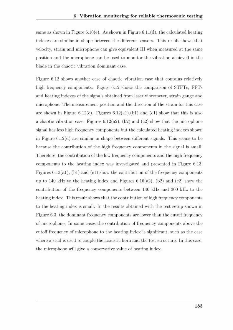
6. Vibration monitoring for reliable thermosonic testing
same as shown in Figure 6.10(e). As shown in Figure 6.11(d), the calculated heating
indexes are similar in shape between the different sensors. This result shows that
velocity, strain and microphone can give equivalent HI when measured at the same
position and the microphone can be used to monitor the vibration achieved in the
blade in the chaotic vibration dominant case.
Figure 6.12 shows another case of chaotic vibration case that contains relatively
high frequency components. Figure 6.12 shows the comparison of STFTs, FFTs
and heating indexes of the signals obtained from laser vibrometer, strain gauge and
microphone. The measurement position and the direction of the strain for this case
are shown in Figure 6.12(e). Figures 6.12(a1),(b1) and (c1) show that this is also
a chaotic vibration case. Figures 6.12(a2), (b2) and (c2) show that the microphone
signal has less high frequency components but the calculated heating indexes shown
in Figure 6.12(d) are similar in shape between different signals. This seems to be
because the contribution of the high frequency components in the signal is small.
Therefore, the contribution of the low frequency components and the high frequency
components to the heating index was investigated and presented in Figure 6.13.
Figures 6.13(a1), (b1) and (c1) show the contribution of the frequency components
up to 140 kHz to the heating index and Figures 6.16(a2), (b2) and (c2) show the
contribution of the frequency components between 140 kHz and 300 kHz to the
heating index. This result shows that the contribution of high frequency components
to the heating index is small. In the results obtained with the test setup shown in
Figure 6.3, the dominant frequency components are lower than the cutoff frequency
of microphone. In some cases the contribution of frequency components above the
cutoff frequency of microphone to the heating index is significant, such as the case
where a stud is used to couple the acoustic horn and the test structure. In this case,
the microphone will give a conservative value of heating index.
183

6. Vibration monitoring for reliable thermosonic testing
6.3.3 The comparison of the heating indexes obtained by
strain on the blade and the clamp
The excitation is usually provided by an ultrasonic horn that is pressed against the
structure. In some cases, as presented in Chapter 4, it is possible to secure the
component to be tested in a clamp. The proposed setup is shown in Figures 4.1
and 6.3 where an ultrasonic horn is attached to a clamp holding the blade. In this
case, a strain gauge can provide a very practical vibration monitoring method when
the strain gauge is positioned on the clamp. Therefore, the heating indexes of the
signals obtained from strain gauges on the clamp and the blade are compared to
evaluate the possibility of monitoring the blade vibration by the strain measured on
the clamp.
Two different cases including fundamental frequency dominant and chaotic were
investigated and examples are presented in Figures 6.14, 6.15 and 6.17. The excita-
tion frequency was 42.8 kHz in these cases which was one of the system resonance
frequencies found before the tests. Figure 6.14 shows the comparison of STFTs and
heating indexes of the signals obtained from strain gauges on the blade and the
clamp in the fundamental frequency dominant case. The measurement positions
of the strain gauges are shown in Figure 6.14(d). The strain gauge on the blade
measured a strain component in direction 1 and the strain gauge on the clamp mea-
sured a strain component in direction 3 at the positions shown in Figure 6.14(d).
Figures 6.14(a) and (b) show that the excited vibration contains the fundamental
frequency component with a small amplitude of the first harmonic. Figure 6.14(c)
shows the comparison of the normalized heating index obtained from the vibration
records measured by strain gauges on the blade and the clamp. As shown in Figure
6.14(c), the calculated heating indexes are very similar in shape. The results pre-
sented above show that the strain measured on the blade and the clamp can give
the equivalent HI in the fundamental frequency dominant case even when measured
at different positions.
Figure 6.15 shows the comparison of STFTs, FFTs and heating indexes of the sig-
184
6. Vibration monitoring for reliable thermosonic testing
nals obtained from strain gauges in a chaotic vibration case. The measurement
positions of the strain gauges and the direction of the strain gauges were the same
as shown in Figure 6.14(d). Figures 6.15(a1) and (b1) show a case where the ex-
cited vibration in the blade is chaotic containing sub harmonics and harmonics of
the excitation frequency and multiple frequency components around the harmonic
frequencies including side bands. Figures 6.15(a2) and (b2) show that strain mea-
sured on the clamp has less high frequency components but the calculated heating
indexes shown in Figure 6.15(c) are similar in shape between different strain signals.
This seems to be because the contribution of the high frequency components in the
strain measured on the blade to the heating index is very small. The contribution of
the low and high frequency components to the heating index was investigated and
presented in Figure 6.16. Figures 6.16(a1) and (b1) show the contribution of the
frequency components up to 100 kHz to the heating index and Figures 6.16(a2) and
(b2) show the contribution of the frequency components between 100 kHz and 300
kHz to the heating index. This result shows that the contribution of high frequency
components to the heating index is small. The result presented above shows that
the strain measured on the blade and the clamp can give the equivalent HI in the
chaotic vibration case even when measured at different positions.
Figure 6.17 shows the result obtained in the test which showed the worst similarity
in the heating index obtained from the strains measured on the blade and the clamp.
Figure 6.17 shows the comparison of STFTs, FFTs and heating indexes of the sig-
nals obtained from strain gauges. Figures 6.17(a1) and (b1) show that this is also a
chaotic vibration case. The measurement positions of the strain gauges and the di-
rection of the strain gauges were the same as shown in Figure 6.14(d). Figure 6.17(c)
shows that there is a discrepancy in the heating indexes obtained from two different
strain signals. This seems to be caused by the different magnitude of frequency
components contained in the signals measured at different positions. In particular,
the FFT of the strain signal measured on the blade shown in Figure 6.17(a2) shows
very high single peak at a frequency around the fundamental frequency. This single
frequency dominant vibration can give different heating indexes at different posi-
tions because the level of measured vibration depends on the measurement position
185

6. Vibration monitoring for reliable thermosonic testing
relative to the mode shape in the single frequency dominant vibration. Therefore
the contribution of the frequency components around the fundamental frequency to
the heating index was investigated. Figure 6.18 shows the comparison of heating
indexes obtained from different frequency ranges. Figure 6.18(a) was obtained from
the frequency components between 0 and 60 kHz and Figure 6.18(b) was obtained
from the frequency components between 60 kHz and 300 kHz. The maximum value
in HI calculated from the frequency components up to 300 kHz was used in the
normalization in Figure 6.18(a) and (b). Figure 6.18 shows that the discrepancy
was mainly caused by the frequency components around the fundamental frequency
that contains a high single peak and this reveals that single frequency dominant
vibration can give different heating indexes in the blade and clamp. This means
that the HI can depend on the measurement position relative to the mode shape
of the dominant mode in the system and in some cases the heating index obtained
from the clamp can lead to the over estimation of the achieved vibration level in the
blade which would reduce the reliability of the test.
6.3.4 The performance of force sensor for vibration moni-
toring
Measurements of force input could provide an indication of frequency content of the
vibration. Therefore, the performance of a force sensor as a vibration monitoring
sensor for thermosonic testing was also investigated when the structure was excited
by an acoustic horn. The problem of the commercial force sensor used in the tests
presented in Chapter 3 is that it operates only up to 30 kHz (-2dB). Therefore, a
new force sensor was made with PZT elements as shown in Figure 6.19. Two ring
type PZT elements with 0.5 mm thickness, 16 mm outer diameter and 5 mm inner
diameter were used for the sensor. The PZT elements were assembled at the end
of the acoustic horn by a steel cap screw with 1 mm thickness and 16 mm head
diameter as shown in Figure 6.19. A thin brass shim with 0.1 mm thickness was
used as an electrode and a wire was soldered on to the electrode. Polyurethane was
used as an encapsulating material in order to provide strain relief for the connection.
186

6. Vibration monitoring for reliable thermosonic testing
Despite this, fatigue was a problem and the fatigue strength needs to be improved
if the idea is to be applied in practice.
Figure 6.20 shows the impedance frequency response of the force sensor assembled
at the end of the acoustic horn. Figure 6.20(a) shows that the frequency response
decreases slowly up to 300 kHz but the resonance frequency is 3.4 MHz which is much
above the frequency range used for thermosonic testing as shown in Figure 6.20(b).
Therefore, the force sensor can be used within the frequency range for thermosonic
testing and if required the frequency response can be used for the compensation
of the frequency components without a difficulty caused by a resonance within the
operating range.
Figure 6.21 shows the comparison of the signal measured by a laser vibrometer and a
force transducer during a test on the steel beam (200×20×20 mm) that was used in
the test shown in Figure 6.8 and Figure 6.9(b). A general purpose amplifier was used
for this test and the excitation frequency was a system resonance frequency of 46.7
kHz. The velocity was measured at the center of the beam. Figures 6.21(a) and (b)
show that the excited vibration shows the characteristics of chaotic vibration with
rich frequency contents. Figure 6.21(c) shows that the normalized heating index is
similar in shape with small difference. The result in Figure 6.21(c) suggests that a
force sensor can be used for the vibration monitoring for thermosonic testing.
Figure 6.22 shows the comparison of the signal measured by a laser vibrometer and
a force sensor during a linear sweep test on a turbine blade. The sweep frequency
range is from 30 kHz to 50 kHz. The blade was secured in a steel clamp and the
acoustic horn was coupled by a spring force. The velocity was measured at the center
of the blade as shown in Figure 6.10(e). Figures 6.22(a2)and (b2) show spectra of
the corresponding signals in Figures 6.22(a1) and (b1). The spectra only show the
frequency range between 30 kHz and 50 kHz. Peaks appear at the frequencies that
correspond to the peaks in Figures 6.22(a1) and (b1). STFTs in Figures 6.22(a3)
and (b3) show very high frequency components around the peak marked 1 in Figures
6.22(a1) and (b1).
187

6. Vibration monitoring for reliable thermosonic testing
Figure 6.23 shows the comparison of the heating indexes calculated from the signals
shown in Figure 6.22. Generally, the shape of the heating index is similar in both
cases and the largest peak appears at the same time which means the same frequency
in a linear sweep test. However, the velocity signal shows two peaks at 1 and 2 but
the force signal shows only one peak at 1. This can be explained by a comparison of
the magnitude and frequency characteristics of both signals. At the peak 1 shown
in Figures 6.22(a1) and (b1), both the velocity and the force are high and more
high harmonics are excited as shown in STFTs in Figures 6.22(a3) and (b3) but
at the peak 2 the velocity is high but the force is small and less high harmonics
are excited as shown in the STFTs. This shows that there is a resonance of the
clamp and blade system. Therefore low force is required to excite it. The position
of the excitation point with respect to the mode shape of the excited mode of the
clamp and blade system can affect the level of response and the force input. The
force depends on how close the excitation point is to a node of the excited mode.
At peak 2 the excitation point seems to be close to an anti-node of the excited
mode and this leads to the result that the response is high but the force is small
at peak 2. This characteristic leads to the disappearance of the second peak in the
heating index calculated from the force signal. In summary, the force sensor can
detect the vibration achieved in the blade up to very high frequency and the velocity
measured by a laser vibrometer on the blade and the force provide a similar shape
of HI when the vibration has a rich frequency content. However, the force signal is
not proportional to the response but it depends on the excitation position relative
to the excited system mode shape. Therefore it could give a false indication of the
vibration achieved in the blade, particulary when a single dominant mode is excited.
It also needs improvement in fatigue strength if the idea is to be applied in practice.
6.4 Mode characteristics in large structures
As presented previously in Chapter 2 and Chapter 4, the vibration field achieved
in a small metal structure showed the characteristic of standing wave modes which
have node points and anti-node points during single frequency excitation. Therefore,
188

6. Vibration monitoring for reliable thermosonic testing
this single mode excitation leads to the existence of blind points for defect detection
at some positions and excitation of multiple modes is required to excite sufficient
vibration over the whole area of the structure. However, large structures may show
different characteristics, especially when the damping is high. When the damping
is high, a standing wave may not be generated so there will be no nodal position.
Therefore, characteristics of the vibration field in the large structures were inves-
tigated to identify the type of mode achieved in tested structures. The tests were
conducted on a composite plate without features, a composite plate with features
and a large steel pipe.
6.4.1 The vibration characteristics in composite structures
Figure 6.24 shows a tested unidirectional CFRP composite plate and the ampli-
tude of the measured velocity along three different paths. Figure 6.24(a) shows the
composite plate with dimensions and three measurement paths. This plate does
not have any features such as ribs and stringers. The out of plane velocity was
measured along the three different paths by a laser vibrometer on a scanning frame
with a measurement interval of 5 mm. A converter of the 40 kHz acoustic horn
(Sonotronic) which has PZT elements inside a steel housing as shown in Figure
6.24(b) was used as an exciter to excite the structure at 40 kHz. The converter was
coupled by using a double sided tape at the center of the plate shown in Figure
6.24(a). Figure 6.24(c) shows the normalized RMS of the velocity measured along
three different paths shown in Figure 6.24(a). It is seen in Figure 6.24(c) that the
amplitude reduces from the excitation point with some oscillation about the trend
but the velocity does not drop to zero at any point and a similar level of attenua-
tion is seen for different directions. This characteristic seems to be caused by high
damping of the composite structure. The results shown in Figure 6.24(c) suggest
that there is no strong standing wave trend and the vibration simply decreases with
distance from the source.
Figure 6.25(a) shows another CFRP composite plate with a rib and stringers; mea-
surement paths 1 and 2 across the rib and stringers are also shown. Figure 6.25(b)
189

6. Vibration monitoring for reliable thermosonic testing
shows the absolute amplitude of the velocity measured along two different paths
shown in Figure 6.25(a). The excitation was at 38.9 kHz that was the frequency
where the resonance was a maximum around the resonance frequency of the exciter
of 40 kHz in this case. The same converter that was used in the test shown in Fig-
ure 6.24 was used in this test and the converter was rigidly bonded at the position
shown in Figure 6.25(a). The general characteristic is similar to that observed in
the composite plate without features shown in Figure 6.24(b); a propagating mode
is dominant, the amplitude reduces with distance from the excitation point and a
similar level of attenuation is seen for different directions. Figure 6.26 shows the
effect of the features shown in Figure 6.25(a) on the measured velocity. Figure
6.26(a) shows that the amplitude at the stringer location is reduced but the stringer
seems to have little effect on the vibration transmission and the amplitude reduces
at all the stringer positions. Figure 6.26(b) shows the vibration amplitude along the
path across the rib. This result shows that the rib also seems to have little effect
on the vibration transmission. In summary, composite structures show a vibration
characteristic where a propagating mode is dominant and there are no node points
in the vibration field even with a single frequency excitation. Therefore, single fre-
quency excitation can be used. The area covered from a single excitation position
is a function of the attenuation, input force, and threshold amplitude required for
damage detection.
6.4.2 The vibration characteristics in large steel structures
A test on a large steel pipe was conducted to see whether a propagating mode
was dominant in the vibration field in the lower damping structure. Figure 6.27(a)
shows the steel pipe used in the test and Figure 6.27(b) shows the absolute vibration
amplitude along the path shown in Figure 6.27(a). The measurement was conducted
on a scanning frame by a laser vibrometer. The excitation frequency for this test was
50.3 kHz and a measurement interval is 2 mm. The converter of the 40 kHz acoustic
horn (Sonotronic) that was used as an exciter for the test of composite structures was
also used to excite the steel pipe structure. The converter was rigidly bonded on the
190

6. Vibration monitoring for reliable thermosonic testing
surface of the steel pipe at the middle of the pipe as shown in Figure 6.27(a). Figure
6.27(b) shows that there is a clear periodicity with no significant decay with position
away from the exciter. The velocity approaches zero periodically; the measurement
spacing was not fine enough to locate the exact nodal position. This result shows
that a standing wave mode can be achieved in a large lower damping structure
such as a steel pipe. Therefore, multiple mode excitation is necessary for reliable
thermosonic testing and the calibration procedure using HI is appropriate.
6.5 Review of Chapter
Vibration monitoring is necessary for reliable thermosonic testing and a Heating
Index (HI) has been proposed as a criterion indicating whether sufficient vibration
is achieved in a tested structure or not. The HI was calculated from different vibra-
tion records measured by different sensors and these results were compared in this
chapter.
Velocity measured by a laser vibrometer and strain provide an equivalent HI when
measured at the same position. The microphone can provide a cheaper vibration
monitoring device than the laser and the heating index calculated by a microphone
signal shows similar characteristics to that calculated from velocity measured by a
laser vibrometer. The microphone frequency response shows that it will underes-
timate high frequency components, so giving a conservative value of HI. The force
sensor can detect the vibration achieved in the testpiece up to very high frequency.
However, the force signal is not proportional to the response but it depends on the
system resonance. Therefore it could give a false indication of the vibration achieved
in the testpiece, particulary when a single dominant system mode is excited. It also
needs improvement in fatigue strength if the idea is to be applied in practice. The
strain measured on the clamp used to hold the component gives a similar form of
heating index to that measured on the component in cases where the vibration has
a rich frequency spectrum. However, differences are seen in cases where a single
mode is dominant.
191

6. Vibration monitoring for reliable thermosonic testing
Testing on large composite structures showed that the material damping is high
enough for standing wave patterns not to be generated and its vibration has a trav-
eling wave characteristic. Therefore, single frequency excitation can be used without
the problem of blind spots. The area covered from a single excitation position is a
function of the attenuation, input force, and threshold amplitude required for dam-
age detection. This is not the case in large steel components. Here, multiple mode
excitation is necessary for reliable thermosonic testing and the calibration procedure
using HI is appropriate.
192

6. Vibration monitoring for reliable thermosonic testing
(a/3)
Freq
. (kH
z)
0 0.2 0.4 0.6 0.80
50
100
150
200
250
-40
-20
0
20
40
dB
(a/2)
Figure 6.1: Heating index and Energy index of the example vibration obtained during the
test excited by horn generator [3]. (a1) Vibration signal; (a2) STFT of the vibration; (a3)
Energy index; (a4) Heating index; (a5) Actual measured temperature rise
193

6. Vibration monitoring for reliable thermosonic testing
Real TestVibration Record*
Thermal Records
Calculate HI from Vibration Record
(using conservative value of k from
calibration)
Detect T rise
HImax ≥ HIth
No Crack
Crack
NO
NO
YES
YES
* The measured vibration must be the same as in the calibration tests, e.g. strain
Legend:action
decision
output
Figure 6.2: Flow chart representing the stages involved in real thermosonics testing [3]
194

6. Vibration monitoring for reliable thermosonic testing
Blade
Clamp
Acoustic Horn
Post
d
Spring
Bolt
Figure 6.3: Schematic of test setup used for the tests to investigate the performance of
different sensors.
195

6. Vibration monitoring for reliable thermosonic testing
Blade
Measurement Position
0 250 500 750 10000
0.2
0.4
0.6
0.8
1
time(ms)
Nor
mal
ized
Hea
ting
Inde
x
Velocity-Blade(mm/s)Strain-Blade(με)
k=30
0 200 400 600 800 10000
50
100
150
200
250
300
Freq
uenc
y(kH
z)
time(ms)-40-30-20-10010203040
Velocity on Blade
dB
(a)
0 200 400 600 800 10000
50
100
150
200
250
300
Freq
uenc
y(kH
z)
time(ms)-40-30-20-100102030
Strain on Blade
dB
(b)
(d)(c)
ε11
Figure 6.4: The comparison of STFTs and heating indexes of the signals obtained from
laser vibrometer and strain gauge in the fundamental frequency dominant case. (a) STFT
of Velocity measured on blade; (b) STFT of strain measured on blade (c) Calculated heating
index (d) Measurement position.
196

6. Vibration monitoring for reliable thermosonic testing
Velocity on Blade
dB
0 500 10000
50
100
150
200
250
300Fr
eque
ncy(
kHz)
time(ms)
-40
-20
0
20
(a1)Strain on Blade
dB
0 500 10000
50
100
150
200
250
300
Freq
uenc
y(kH
z)
time(ms)
-40
-30
-20
-10
0
10
20(b1)
0 250 500 750 10000
0.2
0.4
0.6
0.8
1
time(ms)
Nor
mal
ized
Hea
ting
Inde
x
Velocity-Blade(mm/s)Strain-Blade(με)
k=30(c)
0 50 100 150 200 250 30002468
1012141618
Frequency(kHz)
Am
plitu
de-S
trai
n(μ ε
) (b2)
0 50 100 150 200 250 3000
10
20
30
40
50
60
Frequency(kHz)
Am
plitu
de-V
eloc
ity(m
m/s
)
(a2)
Figure 6.5: The comparison of STFTs and heating indexes of the signals obtained from
laser vibrometer and strain gauge in the chaotic case. (a1) STFT of velocity measured
on blade; (b1) STFT of strain measured on blade (a2) FFT of velocity measured on blade
(b2) FFT of strain measured on blade (c) Calculated heating index.
197

6. Vibration monitoring for reliable thermosonic testing
0 500 10000
50
100
150
200
250
300Fr
eque
ncy(
kHz)
time(ms)
-40
-20
0
20
40
Velocity on Blade
dB
(a1)
0 500 10000
50
100
150
200
250
300
Freq
uenc
y(kH
z)
time(ms)
-40
-20
0
20
Strain on Blade
dB
(b1)
0 250 500 750 10000
0.2
0.4
0.6
0.8
1
time(ms)
Nor
mal
ized
Hea
ting
Inde
x
Velocity-Blade(mm/s)Strain-Blade(με)
(c) k=30
0 50 100 150 200 250 3000510152025303540
Am
plitu
de-S
trai
n(με)
Frequency(kHz)
(b2)(a2)
0 50 100 150 200 250 3000
50
100
150
Frequency(kHz)
Am
plitu
de-V
eloc
ity(m
m/s
)
(a2)
Figure 6.6: The comparison of STFTs and heating indexes of the signals obtained from
laser vibrometer and strain gauge in the chaotic case. ((a1) STFT of velocity measured
on blade; (b1) STFT of strain measured on blade (a2) FFT of velocity measured on blade
(b2) FFT of strain measured on blade (c) Calculated heating index.
198

6. Vibration monitoring for reliable thermosonic testing
Response Vs Distance
0
0.1
0.2
0.3
0.4
0.5
0.6
0.7
0.8
0.9
1
0 20 40 60 80 100 120Distance(mm)
Mic
roph
one
Out
put(V
)Microphone - 4138
Horn tip
Microphone
Distance
Figure 6.7: The characteristic of the microphone; Microphone output voltage vs. distance
from the surface of the tip of the acoustic horn.
Beam
ClampPost
Horn
Microphone
x
Figure 6.8: Schematic of the test setup used for the measurement of the mode shape of
the steel beam (200×20×20 mm) by using a microphone
199

6. Vibration monitoring for reliable thermosonic testing
(b)
-150 -100 -50 0 50 100 150X(mm)
Nor
mal
ized
Am
plitu
de 1mm 120mm
0
0.2
0.4
0.6
1
1.2
0.8
(a)
0
0.2
0.4
0.6
0.8
1
1.2
-150 -100 -50 0 50 100 150X(mm)
Nor
mal
ized
Am
plitu
de
Figure 6.9: Measured mode shape of the steel beam (200×20×20 mm). X is a coordinate
in the direction of the length of the beam; (a) Measured mode shape of the steel beam
obtained by a laser vibrometer during excitation with a PZT exciter coupled with a stud
at the center of the beam under free-free conditions with the test setup shown in Figure
3.1. (b) shows the normalized amplitude of the microphone output voltage along the beam
length at two different distances from the surface of the beam to the microphone, 1 mm
and 120 mm.
200
6. Vibration monitoring for reliable thermosonic testing
Nor
mal
ized
Hea
ting
Inde
x
0 200 400 600 8000
0.2
0.4
0.6
0.8
1
time(ms)
Strain(με)Velocity(mm/s)Microphone(V)
k=30(d)
0 0.5 10
50
100
150
200
250
300
Freq
uenc
y(kH
z)
time(s)
-60
-40
-20
0
20
40
0 0.5 10
50
100
150
200
250
300
Freq
uenc
y(kH
z)
time(s)
-60
-40
-20
0
20
0 0.5 10
50
100
150
200
250
300
Freq
uenc
y(kH
z)
time(s)
-60
-50
-40
-30
-20
-10
0
Velocity Strain Microphone
dBdB
dB(a) (b) (c)
(e)
Strain DirectionMeasurement Position
Figure 6.10: The comparison of STFTs and heating indexes of the signals obtained from
laser vibrometer, strain gauge and microphone in the fundamental frequency dominant
case. (a) STFT of Velocity measured on blade; (b) STFT of strain measured on blade (c)
STFT of microphone output voltage measured on blade (d) Calculated heating index (e)
Measurement position.
201

6. Vibration monitoring for reliable thermosonic testing
0 0.5 10
50
100
150
200
250
300
Freq
uenc
y(kH
z)
time(s)
-60
-40
-20
0
20
0 0.5 10
50
100
150
200
250
300
Freq
uenc
y(kH
z)
time(s)
-60
-50
-40
-30
-20
-10
0
0 0.5 10
50
100
150
200
250
300
Freq
uenc
y(kH
z)
time(s)
-60
-40
-20
0
20
Velocity Strain Microphone
dBdB
dB(a) (b) (c)
time(ms)
Nor
mal
ized
Hea
ting
Inde
x
0 200 400 600 8000
0.2
0.4
0.6
0.8
1
1.2
strain(με)velocity(mm/s)Microphone(V)
k=30(d)
Figure 6.11: The comparison of STFTs and heating indexes of the signals obtained from
laser vibrometer, strain gauge and microphone in the chaotic case. (a) STFT of Velocity
measured on blade; (b) STFT of strain measured on blade (c) STFT of microphone output
voltage measured on blade (d) Calculated heating index.
202

6. Vibration monitoring for reliable thermosonic testing
(a)
0 0.5 10
50
100
150
200
250
300Fr
eque
ncy(
kHz)
time(s)
-60
-40
-20
0
20
40
0 0.5 10
50
100
150
200
250
300
Freq
uenc
y(kH
z)
time(s)
-60
-40
-20
0
20
0 0.5 10
50
100
150
200
250
300
Freq
uenc
y(kH
z)
time(s)
-60
-50
-40
-30
-20
-10
0 100 200 3000
20
40
60
80
100
Frequency(kHz)
Am
plitu
de-V
eloc
ity(m
m/s
)
0 100 200 30005
1015202530
Frequency(kHz)
Am
plitu
de-S
trai
n(με
)
3000 100 2000
0.1
0.2
0.3
0.4
Frequency(kHz)
Am
plitu
de-M
icro
phon
e(V)
0 200 400 600 8000
0.2
0.4
0.6
0.8
1
time(ms)
Nor
mal
ized
Hea
ting
Inde
x
Strain(με)Velocity(mm/s)Microphone(V)
Velocity Strain Microphone(a1)
(c2)(a2)
(b1) (c1)
(b2)
(d)
Measurement Position
Strain Direction
(e)
Figure 6.12: The comparison of STFTs and heating indexes of the signals obtained from
laser vibrometer, strain gauge and microphone in the chaotic case. (a1) STFT of velocity
measured on blade (b1) STFT of strain measured on blade (c1) STFT of microphone
output voltage measured on blade (a2) FFT of velocity measured on blade (b2) FFT of
strain measured on blade (c2) FFT of microphone output voltage measured on blade (d)
Calculated heating indexes. (e) Measurement position.
203

6. Vibration monitoring for reliable thermosonic testing
0 200 400 600 8000
50
100
150
200
250
300
350
time(ms)
Hea
ting
Inde
x
strain(με)(b2)
0 200 400 600 8000
1000
2000
3000
4000
5000
6000
7000
time(ms)
Hea
ting
Inde
x
Velocity(mm/s)(a2)
0 200 400 600 8000
0.02
0.04
0.06
0.08
0.1
time(ms)
Hea
ting
Inde
x
Microphone(V)
0 200 400 600 8000
50
100
150
200
250
300
350
time(ms)
Hea
ting
Inde
x
strain(με)
0 200 400 600 8000
1000
2000
3000
4000
5000
6000
7000
time(ms)
Hea
ting
Inde
x
Velocity(mm/s)
Velocity Strain Microphone(c1)(b1)(a1)
0-140kHz
140-300kHz
0 200 400 600 8000
0.02
0.04
0.06
0.08
0.1
time(ms)
Hea
ting
Inde
x
Microphone(V)(c2)
Figure 6.13: The comparison of heating indexes of the signals obtained from different
sensors in the chaotic case shown in Figure 6.12. (a1) Calculated heating index from
velocity (0-140 kHz) (b1) Calculated heating index from strain (0-140 kHz) (c1) Calculated
heating index from microphone (0-140 kHz) (a2) Calculated heating index from velocity
(140-300 kHz) (b2) Calculated heating index from strain (140-300 kHz)(c2) Calculated
heating index from microphone (140-300 kHz).
204

6. Vibration monitoring for reliable thermosonic testing
Blade
Clamp
Measurement Position
Strain on Blade
dB
0 200 400 600 800 10000
50
100
150
200
250
300
Freq
uenc
y(kH
z)
time(ms)-40-30-20-100102030(a)
(d)
0 250 500 750 10000
0.2
0.4
0.6
0.8
1
time(ms)
Nor
mal
ized
Hea
ting
Inde
x
Strain-Blade(με)Strain-Clamp(με)
k=30(c)
ε33ε11
Strain on Clamp
dB
0 200 400 600 800 10000
50
100
150
200
250
300
Freq
uenc
y(kH
z)
time(ms)-40
-30
-20
-10
0
10(b)
Figure 6.14: The comparison of STFTs and heating indexes of the signals obtained from
strain gauge on blade and clamp in the fundamental frequency dominant case. (a) STFT
of strain measured on blade (b) STFT of strain measured on clamp (c) Calculated heating
index (d) Measurement position.
205

6. Vibration monitoring for reliable thermosonic testing
Strain on Blade(a)
0 500 10000
50
100
150
200
250
300Fr
eque
ncy(
kHz)
time(ms)
-40
-30
-20
-10
0
10
20
dB
(a1)
Strain on Clamp
0 500 10000
50
100
150
200
250
300
Freq
uenc
y(kH
z)
time(ms)
-40
-30
-20
-10
0
10
20
dB
(b1)
0 200 400 600 800 10000
0.2
0.4
0.6
0.8
1
time(ms)
Nor
mal
ized
Hea
ting
Inde
x
Strain-Blade(με)Strain-Clamp(με)
k=30(c)
0 50 100 150 200 250 300024681012141618
Frequency(kHz)
Am
plitu
de-S
trai
n(με) (a2)
0 50 100 150 200 250 30000.51
1.52
2.53
3.54
Am
plitu
de-S
trai
n(μ ε
)
Frequency(kHz)
(b2)
Figure 6.15: The comparison of STFTs and heating indexes of the signals obtained from
strain gauges on blade and clamp in the chaotic case. (a1) STFT of strain measured on
blade (b1) STFT of strain measured on clamp (a2) FFT of strain measured on blade (b2)
FFT of strain measured on clamp (c) Calculated heating index.
206
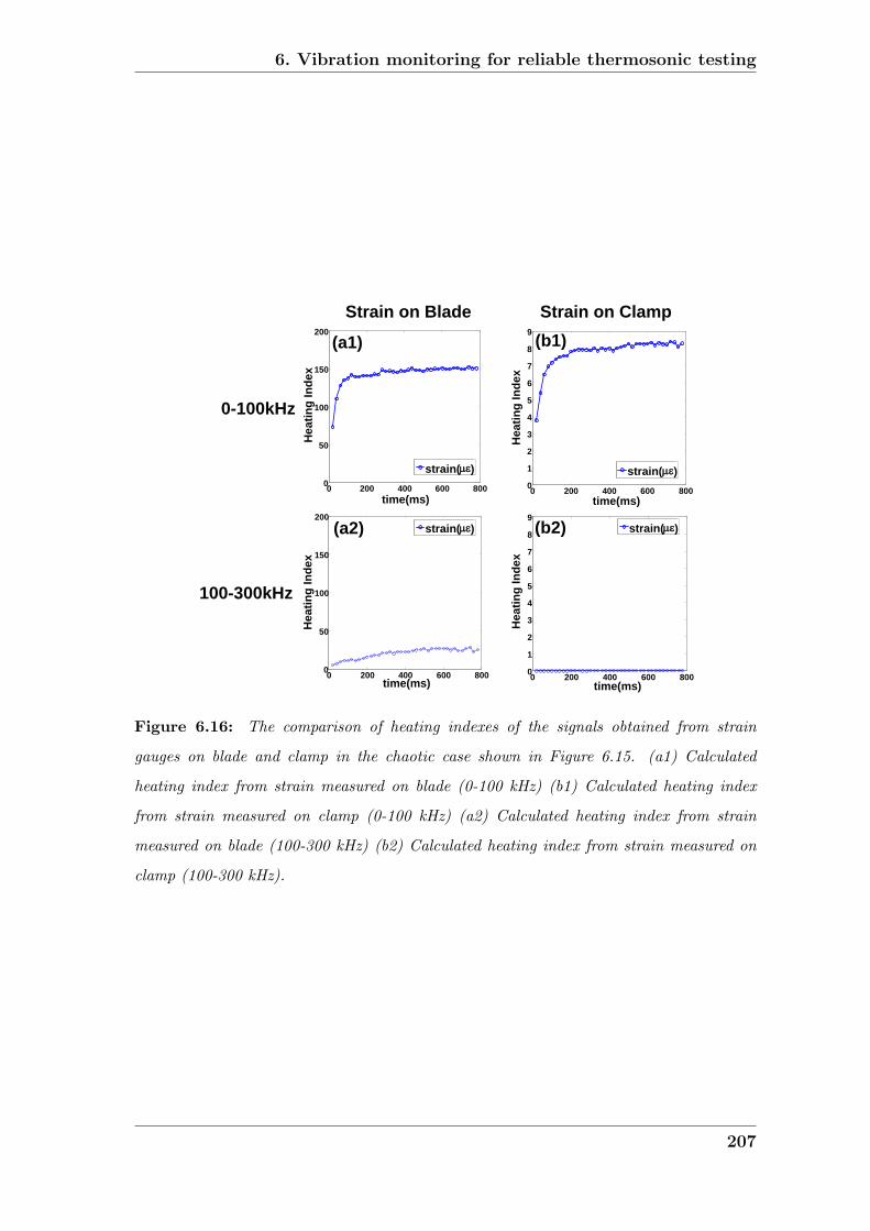
6. Vibration monitoring for reliable thermosonic testing
time(ms)
(a)
100-300kHz
0-100kHz
20ms
Strain on Blade Strain on Clamp
0 200 400 600 8000
50
100
150
200
time(ms)
Hea
ting
Inde
x
strain(με)
strain(με)
0 200 400 600 8000
1
2
3
4
5
6
7
8
9
time(ms)H
eatin
g In
dex
strain(με)
Hea
ting
Inde
x
(b1)(a1)
0 200 400 600 8000
1
2
3
4
5
6
7
8
9
time(ms)
Hea
ting
Inde
xstrain(με)
0 200 400 600 8000
50
100
150
200strain(με)
Str : -0.1
(a2) (b2)
Figure 6.16: The comparison of heating indexes of the signals obtained from strain
gauges on blade and clamp in the chaotic case shown in Figure 6.15. (a1) Calculated
heating index from strain measured on blade (0-100 kHz) (b1) Calculated heating index
from strain measured on clamp (0-100 kHz) (a2) Calculated heating index from strain
measured on blade (100-300 kHz) (b2) Calculated heating index from strain measured on
clamp (100-300 kHz).
207

6. Vibration monitoring for reliable thermosonic testing
Strain on Blade
(a)
0 500 10000
50
100
150
200
250
300Fr
eque
ncy(
kHz)
time(ms)
-40
-20
0
20
dB
(a1)Strain on Clamp
0 500 10000
50
100
150
200
250
300
Freq
uenc
y(kH
z)
time(ms)
-40
-30
-20
-10
0
10
20
dB
(b1)
k=30
0 250 500 750 10000
0.2
0.4
0.6
0.8
1
time(ms)
Nor
mal
ized
Hea
ting
Inde
x
Strain-Blade(με)Strain-Clamp(με )
(c) k=30
0 50 100 150 200 250 3000510152025303540
Am
plitu
de-S
trai
n(με)
Frequency(kHz)
(a2)
0 50 100 150 200 250 30000.5
11.5
22.5
33.5
4
Am
plitu
de-S
trai
n(με)
Frequency(kHz)
(b2)
Figure 6.17: The comparison of STFTs and heating indexes of the signals obtained from
strain gauges on blade and clamp in the case which showed the worst similarity in the
heating index obtained from the strains measured on the blade and the clamp. (a1) STFT
of strain measured on blade (b1) STFT of strain measured on clamp (a2) FFT of strain
measured on blade (b2) FFT of strain measured on clamp (c) Calculated heating index.
208

6. Vibration monitoring for reliable thermosonic testing
0-60 60-300
0 200 400 600 800 10000
0.1
0.2
0.3
0.4
0.5
0.6
0.7
0.8
0.9
1
time(ms)
Hea
ting
Inde
x
Strain-Blade(με)Strain-Clamp(με)
60-100 100-300
0 200 400 600 800 10000
0.10.20.30.40.50.60.70.80.91
time(ms)
Strain-Blade(με)Strain-Clamp(με)
Nor
mal
ized
Hea
ting
Inde
x (b)
0 200 400 600 800 10000
0.10.20.30.40.50.60.70.80.9
1
time(ms)
Strain-Blade(με)Strain-Clamp(με)
Nor
mal
ized
Hea
ting
Inde
x (a)
Figure 6.18: The comparison of heating indexes of the signals obtained from strain gauges
on blade and clamp in the chaotic case shown in Figure 6.17. (a) Calculated normalized
heating index from strain (0-60 kHz) (b) Calculated normalized heating index from strain
(60-300 kHz).
209

6. Vibration monitoring for reliable thermosonic testing
-
16mm
1mm
PZTPZT Thickness = 0.5mm
Acoustic Horn
+
WireEncapsulating MaterialSoldering Point
Cap Screw
Figure 6.19: Schematic of the PZT force sensor assembled at the end of the acoustic
horn.
100
1000
10000
100000
1000000
10000000
0 100 200 300 400 500 600
Frequency(kHz)
Impe
danc
e(Ω
)
(a)
1
10
100
1000
10000
100000
1000000
10000000
0 2 4 6 8 1 1.2 1.4 1.6
Frequency(MHz)
Impe
danc
e(Ω
)
(b)
Figure 6.20: Impedance frequency response of the force sensor assembled at the end of the
acoustic horn. (a) Impedance frequency response up to 500 kHz; (b)Impedance frequency
response up to 1.5 MHz
210

6. Vibration monitoring for reliable thermosonic testing
0 0.5 10
0.2
0.4
0.6
0.8
1
time(s)
Nor
mal
ized
Hea
ting
Inde
x
Force Voltage(V)velocity(mm/s)
20ms
0 0.5 10
50
100
150
200
250
300
Freq
uenc
y(kH
z)
time(s)
-60
-40
-20
0
0 0.5 10
50
100
150
200
250
300
Freq
uenc
y(kH
z)
time(s)
-60
-50
-40
-30
-20
-10
0
Velocity Force
dB
dB(a) (b)
(c)
Figure 6.21: Comparison of the signal measured by laser vibrometer and force transducer
during the test on the beam(200×20×20 mm); (a)STFT of velocity (mm/s) (b)STFT of
force sensor output voltage (V) (c)Heating index
211

6. Vibration monitoring for reliable thermosonic testing
0 0.5 10
50
100
150
200
250
300
Freq
uenc
y(kH
z)
time(s)
-60
-50
-40
-30
-20
-10
0
0 0.5 10
50
100
150
200
250
300
Freq
uenc
y(kH
z)
time(s)
-60
-40
-20
0
20
0 200 400 600 800 1000-200
-100
0
100
200
Velo
city
(mm
/s)
time(ms)
(a1) 12
dB
dB(b3)
30 35 40 45 500
0.01
0.02
0.03
0.04
0.05
Frequency(kHz)
Forc
e Vo
ltage
(V) 1
2
(b2)
0 200 400 600 800 1000-10
-5
0
5
10
Forc
e Vo
ltage
(V)
time(ms)
(b1) 1
2
30 35 40 45 500
0.2
0.4
0.60.8
1
Frequency(kHz)Am
plitu
de-V
eloc
ity(m
m/s
)
(a2) 1
2
(a3)
Figure 6.22: Comparison of the signal measured by laser vibrometer and force sensor
during a linear sweep test on a turbine blade. (a1) Velocity, (a2) Spectrum of the velocity,
(a3) STFT of the velocity, (b1) Force sensor output voltage, (b2) Spectrum of the force
sensor output voltage, (b3) STFT of the force sensor output voltage
212

6. Vibration monitoring for reliable thermosonic testing
(a)0 500 10000
0.2
0.4
0.6
0.8
1
time(ms)
Nor
mal
ized
Ene
rgy
Inde
x Force Voltage(V)Velocity(mm/s)
(b)0 500 10000
0.2
0.4
0.6
0.8
1
time(ms)
Nor
mal
ized
Hea
ting
Inde
x Force Voltage(V)Velocity(mm/s)
k=301
2
0 500 10000
0.2
0.4
0.6
0.8
1
time(ms)
Nor
mal
ized
Hea
ting
Inde
x Force Voltage(V)Velocity(mm/s) 1
2
Figure 6.23: Comparison of heating indexes calculated from the signal measured by laser
vibrometer and force sensor during a sweep test on a turbine blade.
213

6. Vibration monitoring for reliable thermosonic testing
Exciter Position
2
1165
940
t = 3.7mm
1 3
(c)
(a)
100 200 300 400 500 600 700
0.1
0.2
0.3
0.4
0.5
0.6
0.7
0.8
0.9
1
Distance from center(mm)
Nor
mal
ized
RM
S of
Vel
ocity
(mm
/s)
123
(b)
Figure 6.24: Tested composite plate and amplitude of the measured velocity. (a) CFRP
composite plate and measurement paths; (b) Converter; (c) Normalized RMS of the velocity
measured along three different paths shown in Figure 6.24(a). Excitation frequency: 40
kHz, Measurement interval: 5 mm.
214

6. Vibration monitoring for reliable thermosonic testing
Exciter Position
1
2Stringer
Rib
0
10
20
30
40
50
60
0 200 400 600 800 1000 1200 1400 1600Distance(mm)
Velo
city
(mm
/s)
Composite Plate(1700mm X 1782mm) - Skin: t=7mm, Stringer: t=10mm, Rib: t=5mm
(a) (b)
Skin(t=7mm)
Rib(t=5mm)Stringer(t=10mm)
21
1700
1782
Figure 6.25: Tested composite plate and amplitude of the measured velocity. (a) CFRP
composite plate and measurement paths; (b) Amplitude of velocity measured along two
different paths shown in Figure 6.25(a). Excitation frequency: 40 kHz, Measurement
interval: 5 mm.
0
10
20
30
40
50
60
0 200 400 600 800 1000 1200 1400 1600
Distance(mm)
Velo
city
(mm
/s)
- No node points
- Amplitude is reduced around a stringer
0
10
20
30
40
50
60
0 200 400 600 800Distance(mm)
Velo
city
(mm
/s) 1
Stringer
2
Rib
Composite Plate(1200mm X 1782mm)
(b)(a)
Figure 6.26: The effect of features shown in Figure 6.25(a) on the amplitude of the
measured velocity. (a)Vibration amplitude through the stringers; (b)Vibration amplitude
through a rib. Excitation frequency: 38.9 kHz.
215

6. Vibration monitoring for reliable thermosonic testing
Laser Scanning(2mm step)
Exciter Position
(Middle of the length)
0 50 100 150 200 250 300 350 400 450 5000
10
20
30
40
50
60
70
80
90
Distance From Excitation Point(mm)
Velo
city
(mm
/s)
λ = 36mm
(b)
(a)
Thickness: t = 8.2mmLength: L = 1mInside Diameter: 203.6mm
Figure 6.27: Vibration amplitude along the steel pipe. (a) steel pipe; (b) Vibration
amplitude along the measurement path shown in Figure 6.27(a). Excitation frequency:
50.3 kHz, Measurement interval: 2 mm.
216

Chapter 7
Conclusions and further work
7.1 Review of thesis
Thermosonics is a non-destructive testing method in which cracks or damage in an
object are made visible through frictional heating caused by low-frequency ultra-
sound. The heat is generated through the dissipation of mechanical energy at the
crack interfaces by vibration. The frequency range used for excitation of structures
is typically from 20 kHz to 100 kHz. The presence of a crack will result in a tem-
perature rise around the area and the surface close to the crack. The temperature
rise is measured by a high sensitivity infrared imaging camera whose field of view
covers the whole component. The method therefore covers the whole component
from a single excitation position so it is much quicker than conventional ultrasonic
or eddy current inspection that requires scanning over the whole surface and also can
be a more convenient and reliable inspection technique for structures with complex
geometries that are difficult to inspect by conventional methods.
Thermosonics benefits from the non-linearities caused by the contact between the
specimen and the supports and between the specimen and the exciter. A rich spec-
trum of vibration caused by the non-linearities improves the temperature rise in
thermosonic testing. However, the reliable inspection of defects by thermosonics is
very difficult because of the lack of repeatability and consistency of the thermosonic
217
7. Conclusions and further work
signal(surface temperature rise) caused by the non-linearity in the coupling. There-
fore, a study to develop a reliable excitation method which can generate control-
lable vibration in the test structure is required for the application of thermosonics
as a reliable NDT technique. This thesis investigates the use of a Langevin type
piezoelectric transducer as a controllable excitation source, as a alternative to the
commonly used ultrasonic horn. Many aspects of the problems in the existing horn
system are related to the interface force in the system as discussed in Chapter 1.
Therefore, the frequency characteristics of the system comprising the test structure
and a PZT exciter was studied by the finite element method to evaluate the level
of strain excited in a test structure and the interface force between the exciter and
the test structure in Chapter 2. The prediction was validated by experiments in
Chapter 3. The strain induced in the structure and the dynamic interface force
between the exciter and the structure were measured as a function of frequency for
a range of exciter designs and coupling methods. The tests were conducted on steel
beams, steel plates and composite plates. The frequency response characteristics of
strain and interface force obtained by the finite element method were also compared
with the experimental results.
One of the important advantages of Thermosonics is that it can be applied to com-
plex structures such as a turbine blade as a convenient and quick screening test
method. For a reliable thermosonic test, the vibrational characteristics of the sys-
tem comprising the test structure and the excitation system should be identified.
The characteristics of vibration produced in simple structures such as beams and
plates with simple PZT exciters were presented in Chapter 2 and Chapter 3. How-
ever, the vibration characteristics in complex structures such as turbine blades are
more complicated and must be investigated to prepare a reliable thermosonic test
procedure. Therefore, the vibration characteristics in a complex structure such as
a turbine blade were described in Chapter 4. A practical thermosonic test setup
which secures a test component in a clamp and attaches a horn to the clamp via a
stud was also presented. The feasibility of the prediction of mode characteristics in
complex structures such as turbine blades was also discussed.
218

7. Conclusions and further work
Several studies have shown that a rich spectrum of vibration greatly improves the
temperature rise in thermosonic testing [2, 43, 90]. It was also shown in Chapters
2 and 3 that multiple mode excitation is required to obtain enough strain over the
whole structure for reliable thermosonic testing [40,41,91]. Therefore, the influence
of the clamping method and the excitation signal that is input to the horn on the
vibration characteristics are studied experimentally and presented in Chapter 5. A
fast narrow band sweep test with a general purpose amplifier and stud coupling is
presented as an excitation method. This method can be applied to different types
of turbine blades and also to other components.
A numerical method is very attractive to decide which mode should be used and
what excitation level is required to obtain sufficient vibration over the whole area of
the tested structure. However, the mode prediction procedure for a complex struc-
ture such as a blade and clamp system is not reliable as presented in Chapter 4.
One typical characteristic of a thermosonic test is the lack of repeatability in the
amplitude and the frequency characteristic of the vibration. This means vibration
monitoring is necessary to decide whether sufficient vibration is achieved in tested
structures during each test and the vibration level should be compared with the
required vibration level for reliable crack detection which can be obtained in cali-
bration tests. Therefore, a calibration test procedure is required to find the required
vibration level for the reliable detection of the target defects.
In Chapter 6 a calibration procedure for reliable thermosonic testing and a heating
index [3, 14] calculated from a measured vibration record which could be a param-
eter indicating whether sufficient excitation had been applied were reviewed. The
performance of different sensors for vibration monitoring for reliable thermosonic
testing was investigated. Sensors investigated included a laser vibrometer, a micro-
phone and a force sensor that can provide a vibration record which can be used to
calculate the heating index. The characteristics of the vibration in large structures
were also investigated to evaluate the appropriateness of the heating index.
219

7. Conclusions and further work
7.2 Summary of Findings
The work on thermosonics undertaken in this Thesis has led to an extensive quanti-
tative and qualitative assessment of the excitation methods for thermosonic testing.
A numerical and experimental study for the development of the excitation method
for reliable thermosonic testing is presented in this thesis. Successful excitation
methods for the detection of delaminations in composites and cracks in metal struc-
tures are described.
7.2.1 Design of reproducible exciter
- Modelling of the system comprising PZT exciter and structure
In this thesis, a finite-element-based computational model has been used successfully
to predict the frequency responses of coupled systems of a piezo exciter and steel
structures such as beams and plates. The frequency response characteristics of
interface force and strain were successfully predicted. This numerical work provided
a better understanding of the influence of the coupling between the exciter and the
testpiece and also made it possible to evaluate the strain excited in the specimen
and the interface force between the exciter and the testpiece. It also provided a
detailed understanding of the influence of different excitation parameters on system
response.
- Dynamic interface force and system response
As explained in Chapter 1, if the static coupling force is smaller than the dynamic
interface force, loss of contact causes chattering which produces an uncontrollable
non-linear vibration in the tested structure. Therefore, the characteristics of the
interface force were studied to develop a reliable and consistent excitation system.
Generally, the interface force maximum occurs at the strain maximum. Therefore
the force is high at the strain resonance and this may cause a loss of contact in
practice. Tuning can reduce the dynamic interface force, but a problem is that the
220
7. Conclusions and further work
exciter resonance frequency is very sensitive to the total length of the exciter. This
makes tuning to a particular mode frequency very difficult in practice.
The excitation system should excite enough strain over the whole area of the struc-
ture to detect defects at different positions in the structure. However, single mode
excitation leads to the possibility of vibrational nodes at some potential defect loca-
tions. Therefore several modes need to be excited in order to obtain sufficient strain
over the whole area of the structure for reliable damage detection. If the mode den-
sity is high near the exciter resonance frequency, several modes can be excited by
a small interface force that makes it possible to achieve sufficient and reproducible
vibration in a test structure.
If it is intended to use reproducible vibration for reliable thermosonic testing, suffi-
cient strain levels should be achieved in the test structure before the interface force
reaches the limit value that causes loss of contact between the exciter and the test
structure. The strain level obtained using a wax coupled simple PZT exciter was 73
µε on a 4 mm thick steel plate and 55 µε on a 5 mm thick steel plate at an input volt-
age of 125V. These results show that a reproducible vibration may be sufficient for
thermosonic testing in some metal structures such as thin plates. However strain
levels over 50 µε are often required in metal structures [14], though the required
strain level is dependent on a crack size. This level of strain is not easily achieved
within the reproducible vibration range because the interface force limit is reached
first.
- The influence of the damping on the system response
The influence of the damping characteristics of the structure on the excited strain
and the interface force was studied by FEM analysis of a steel beam. If the damping
of the structure increases, the dynamic interface force per unit input voltage at the
resonances decreases, and there is a relatively small difference of dynamic interface
force between the tuned and non-tuned conditions. This effectively makes the system
broader band and will allow excitation of several closely spaced modes at similar
amplitudes. However, the increase of damping also causes a decrease of the excited
221

7. Conclusions and further work
strain per unit input voltage, so to obtain a given strain, higher voltage input is
required; this required voltage level depends on the required strain level for damage
detection.
- The performance of a simple PZT exciter
Generally, short pulses whose pulse duration is below 1 sec have been used for
thermosonics. However, in composites, it has been shown that low power input with
a longer pulse time can be used. This greatly reduces the dynamic interface force
and so reduces the possibility of damage at the exciter position caused by chattering.
The simple PZT exciter developed here has been shown to be suitable for this long
pulse excitation. Another advantage of the low power requirement for long pulse
thermosonics is that it is possible to use a lightweight portable system such as a
simple PZT exciter.
7.2.2 Multiple mode excitation system
- Needs for multiple mode excitation
The key concern for reliable thermosonic testing is not to achieve the maximum
strain response at some specific location, but rather to maximise the minimum
strain response achieved at any of the positions of interest. Therefore, if standing
wave modes are excited, more than two modes should be excited to obtain sufficient
strain at the node points of a single mode. This is easily achieved with non-linear
vibration, but at a cost of reduced reproducibility and reliability.
- Comparison of stud and spring coupling
In some cases it is possible to secure the component to be tested in a clamp and
to attach the horn to the clamp via a stud or simply by pressing the horn against
the clamp. The experimental results with a turbine blade in a clamp show that
the transfer of vibration from the horn to the blade via the clamp is sufficient for
the detection of cracks in the blade. The stud coupling generally generates higher
amplitude vibration than spring force coupling. The vibration shows very high
222

7. Conclusions and further work
responses at around the lowest impedance frequency especially in the stud coupling
case. In the spring force coupling case which shows relatively high impedance over
a wide frequency range, impedance matching can improve the power transfer to the
load side and produce higher vibration levels in the test structure.
- Performance of chirp test for multiple mode excitations
A higher response can be obtained if the excitation frequency coincides with the
resonances of the system comprising the component and the excitation system. This
has been achieved by employing a chirp input over a frequency range centered on the
system resonance frequency. Significant vibration amplitudes are then seen at the
system resonances which coincide with multiples of the excitation frequencies in the
frequency range of the chirp. At some frequencies within the chirp frequency range,
chaotic vibration is achieved and multiple modes around the excitation frequency
and the harmonics of the excitation frequency were excited. This rich spectrum of
vibration can improve the temperature rise and crack detectability over the area of
the test structure. Another advantage of the chirp test is that it does not require a
tuning procedure.
Thermosonic testing is often done using the generator that is supplied with an
acoustic horn. While the input frequency is nominally at the resonance frequency of
the horn, the amplifier does hunt for the true resonance so it is not a fixed frequency
device. A fast narrow band sweep test with a general purpose amplifier and stud
coupling has been proposed as an alternative excitation method for thermosonic
testing. This method can be applied to different types of turbine blades and also to
other components.
7.2.3 Calibration test and Vibration monitoring
- Reliability of prediction procedure
If the vibration achieved in a test structure is reproducible, it could be very attrac-
tive to use a numerical prediction procedure to decide which modes should be used
223

7. Conclusions and further work
and what excitation level is required to obtain sufficient vibration over the whole
area of the tested structure. However, the mode prediction procedure for a complex
structure such as a blade and clamp system was shown to be unreliable. The differ-
ence between prediction and experiments seems to be caused by uncertainties in the
model, including the interface between the clamp and the blade. The mode shapes
around the interface are also very complicated at high frequencies where the modal
density is also high.
- Needs for calibration test and vibration monitoring
One typical characteristic of a thermosonic test using non-linear vibration is the lack
of repeatability in the amplitude and the frequency characteristic of the vibration.
This means vibration monitoring is necessary to decide whether sufficient vibration
is achieved in the tested structure. The vibration level should be compared with
the required vibration level for reliable crack detection which can be obtained in
calibration tests. Therefore, a calibration test procedure is required to find the
required vibration level for the reliable detection of the target defects. A Heating
Index (HI) [3] has been proposed as a criterion indicating whether sufficient vibration
is achieved in a tested structure or not. The HI can be calculated from different
vibration records measured by different sensors.
- Performance of different sensors for vibration monitoring
Velocity measured by a laser vibrometer and strain provide an equivalent HI when
measured at the same position. The microphone can provide a cheaper vibration
monitoring device than the laser and the heating index calculated by a microphone
signal shows similar characteristics to that calculated from velocity measured by a
laser vibrometer. The microphone frequency response shows that it will underes-
timate high frequency components, so giving a conservative value of HI. A force
sensor can detect the vibration achieved in the testpiece up to very high frequency.
However, the force signal is not proportional to the response but it depends on the
system resonance. Therefore it could give a false indication of the vibration achieved
in the testpiece, particulary when a single dominant system mode is excited. It also
224

7. Conclusions and further work
needs improvement in fatigue strength if the idea is to be applied in practice. The
strain measurement on the clamp used to hold the component gives a similar form
of heating index to that measured on the component in cases where the vibration
has a rich frequency spectrum. However, differences are seen in cases where a single
mode is dominant.
- Appropriateness of HI for large structures
Testing on large composite structures showed that the material damping is high
enough for a standing wave pattern not to be generated and its vibration has a trav-
eling wave characteristic. Therefore, single frequency excitation can be used without
the problem of blind spots. The area covered from a single excitation position is a
function of the attenuation, input force, and threshold amplitude required for dam-
age detection. This is not the case in large steel components. Here, multiple mode
excitation is necessary for reliable thermosonic testing and the calibration procedure
using HI is appropriate.
7.3 Further work
Further work could be done to develop a practical and convenient test system that
can be directly applied to real structures. Some more engineering work is needed
to develop a compact portable thermosonic test system. It also requires the de-
velopment of efficient software for the automation of the whole thermosonic test
procedure.
It has been shown that vibration monitoring is necessary for reliable thermosonic
testing and a Heating Index (HI) has been proposed as a criterion indicating whether
sufficient vibration is achieved in a tested structure or not. The applicability of the
calibration and test procedure using HI to real tests with diverse complicated struc-
tures will be investigated. These work includes the investigation of the relationship
between Heating Index and detectability of cracks at unknown positions. Testing on
different complex structures is also needed to investigate whether a heating index
225

7. Conclusions and further work
measured at one point can be used as a measure of defect detectability over the
whole structure.
The HI calculated from different vibration records measured by different sensors are
compared in Chapter 6 and these results proposed several promising sensors for the
vibration monitoring. However, more work is required to find an optimal sensor and
measurement position that can provide a Heating Index satisfactorily representing
temperature rise at different crack positions. Therefore, further work will also be
done to compare the temperature rise at a crack and the Heating Index calculated
from different vibration records measured by different sensors at different positions to
find the optimal vibration measurement method. The test results shown in Chapter
5 show that sweeping the excitation over a frequency range could excite multiple
modes and cover a large area of structure. Further work is needed to compare the
performance of the pulsed excitation with the excitation by sweeping the excitation
over a frequency range on the same specimen to investigate detectability of cracks
at unknown positions.
226

References
[1] “Engine failure: Boeing 717-200,” Aviation Safety Investigation Report (Aus-
tralian transport safety bureau, http://www.atsb.gov.au/publications/, 2006).
[2] X. Y. Han, Z. Zeng, W. Li, M. S. Islam, J. P. Lu, V. Loggins, E. Yitamben, L. D.
Favro, G. Newaz, and R. L. Thomas, “Acoustic chaos for enhanced detectability
of cracks by sonic infrared imaging,” Journal of Applied Physics 95(7), 3792–
3797 (2004).
[3] M. Morbidini, “A comparison of the vibration-modulation and thermosonic
ndt techniques,” Ph.D. thesis, Imperial College, University of London, 2007,
mechanical Engineering.
[4] C. Hellier, Handbook of Nondestructive Evaluation (McGraw Hill, New York -
London, 2001).
[5] X. Maldague, Nondestructive Evaluation of Materials by Infrared Thermogra-
phy (Springer-Verlag, London, 1993).
[6] X. Maldague, in Trends in Optical Nondestructive Testing and Inspection,
edited by P. K. Rastogi and I. Inaudi (Elsevier Science, New York, 2000),
Chap. Application of infrared thermography in nondestructive evaluation (in-
vited chapter), pp. 591–609.
227
REFERENCES
[7] D. Almond, G. Busse, E. Grinzato, J. C. Krapez, X. Maldague, V. Vavilov,
and W. Peng, “Infrared thermographic detection and characterization of im-
pact damages in carbon fiber plastics: round robin test result,” in Proceedings
of QIRT98 (Quantitative Infrared Thermography 1998), Lodz, Poland, 7-10
September 1998, edited by D. Balageas, G. Busse, and G. Carlomagno (Polish
Society of Optoelectronic Engineering, Warszawa, Poland, 1998), Eurotherm
Seminar 60.
[8] L. D. Favro, X. Y. Han, Z. Ouyang, G. Sun, H. Sui, and R. L. Thomas, “Infrared
imaging of defects heated by a sonic pulse,” Review of Scientific Instruments
71(6), 2418–2421 (2000).
[9] X. Y. Han, L. D. Favro, Z. Ouyang, and R. L. Thomas, “Thermosonics: De-
tecting cracks and adhesion defects using ultrasonic excitation and infrared
imaging,” Journal of Adhesion 76(2), 151–162 (2001).
[10] A. Gleiter, G. Riegert, T. Zweschper, and G. Busse, “Ultrasound lockin ther-
mography for advanced depth resolved defect selective imaging,” in Euro-
pean Conference on Nondestructive Testing, ECNDT Conference Proceedings
(Berlin, Germany, 25-29 September, 2006).
[11] R. L. Thomas, L. D. Favro, X. Han, Z. Ouyang, H. Sui, and G. Sun, Infrared
imaging of ultrasonically excited subsurface defects in materials, US PATENT
APPLICATION number 6236049, 1999.
[12] P. Cawley and D. P. Almond, Thermosonics - A New Quick Technique for Crack
Detection, 2002, case for support.
[13] P. Cawley and D. P. Almond, Compact thermosonic NDE system, 2006, case
for support.
228

REFERENCES
[14] M. Morbidini, P. Cawley, T. Barden, and D. Almond, “Prediction of the ther-
mosonic signal from fatigue cracks in metals using vibration damping measure-
ments,” Journal of Applied Physics 100(10), 1–13 (2006).
[15] C. J. Pye and R. D. Adams, “Heat emission from damaged composite materials
and its use in nondestructive testing,” Journal of Physics D-Applied Physics
14(5), 927–941 (1981).
[16] C. J. Pye and R. D. Adams, “Detection of damage in fiber reinforced plastics us-
ing thermal fields generated during resonant vibration,” NDT&E International
14(3), 111–118 (1981).
[17] R. D. Adams, P. Cawley, C. J. Pye, and B. J. Stone, “Vibration technique
for non-destructively assessing integrity of structures,” Journal of Mechanical
Engineering Science 20(2), 93–100 (1978).
[18] R. D. Adams and P. Cawley, “Vibration techniques in nondestructive testing,”
in Research Techniques in Nondestructive Testing, edited by R. S. Sharpe (Aca-
demic Press Inc. Ltd., London, 1985), Vol. 8, Chap. 7, pp. 304–360.
[19] R. B. Mignogna and R. E. Green, “Multiparameter system for investigation of
the effects of high-power ultrasound on metals,” Review of Scientific Instru-
ments 50(10), 1274–1277 (1979).
[20] R. B. Mignogna, R. E. Green, J. C. Duke, E. G. Henneke, and K. L. Reifsnider,
“Thermographic investigation of high-power ultrasonic heating in materials,”
Ultrasonics 19(4), 159–163 (1981).
[21] R. L. Thomas, “Thermal NDE techniques - from photoacoustics to thermoson-
ics,” in Review of Progress in Quantitative Nondestructive Evaluation 21,
Vol. 615 of AIP Conference Proceedings, edited by D. O. Thompson and D. E.
Chimenti (American Institute of Physics, Melville, NY, 2002), pp. 3–13.
229
REFERENCES
[22] D. Wu, A. Salerno, J. Rantala, and G. Busse, “Characterization of layered
materials using lock-in thermography,” Progress in Natural Science 6, 76–79
(1996), suppl. S.
[23] D. T. Wu and G. Busse, “Lock-in thermography for nondestructive evaluation
of materials,” Revue Generale De Thermique 37(8), 693–703 (1998).
[24] J. Rantala, D. Wu, and G. Busse, “Amplitude-modulated lock-in vibrother-
mography for NDE of polymers and composites,” Research in Nondestructive
Evaluation 7(4), 215–228 (1996).
[25] J. Rantala, D. Wu, and G. Busse, “NDT of polymer materials using lock-in
thermography with water-coupled ultrasonic excitation,” NDT&E International
31(1), 43–49 (1998).
[26] T. Zweschper, A. Dillenz, and G. Busse, “Ultrasound lock-in thermography -
a defect-selective NDT method for the inspection of aerospace components,”
Insight 43(3), 173–179 (2001).
[27] T. Zweschper, A. Dillenz, G. Riegert, D. Scherling, and G. Busse, “Ultrasound
excited thermography using frequency modulated elastic waves,” Insight 45(3),
178–182 (2003).
[28] A. Dillenz, T. Zweschper, and G. Busse, “Elastic wave burst thermography for
NDE of subsurface features,” Insight 42(12), 815–817 (2000).
[29] T. Zweschper, A. Dillenz, G. Riegert, and G. Busse, “Ultrasound burst phase
thermography(UBP) for applications in the automotive industry,” in Review
of Progress in Quantitative Nondestructive Evaluation 22, Vol. 657 of AIP Con-
ference Proceedings, edited by D. O. Thompson and D. E. Chimenti (American
Institute of Physics, Melville, NY, 2003), pp. 531–536.
230
REFERENCES
[30] L. D. Favro, X. Y. Han, O. Y. Zhong, G. Sun, and R. L. Thomas, “Sonic
IR imaging of cracks and delaminations,” Analytical Sciences 17, S451–S453
(2001), sp. Iss. SI.
[31] L. D. Favro, R. L. Thomas, X. Han, Z. Ouyang, G. Newaz, and D. Gentile,
“Sonic infrared imaging of fatigue cracks,” International Journal of Fatigue 23,
S471–S476 (2001), suppl. S.
[32] L. D. Favro, X. Y. Han, Z. Ouyang, L. Li, S. Wang, and R. L. Thomas, “Ther-
mosonic imaging of cracks and delaminations,” Progress in Natural Science 11,
S133–S136 (2001), suppl. S.
[33] X. Y. Han, L. D. Favro, and R. L. Thomas, “Recent developments in sonic IR
imaging,” in Review of Progress in Quantitative Nondestructive Evaluation 22,
Vol. 657 of AIP Conference Proceedings, edited by D. O. Thompson and D. E.
Chimenti (American Institute of Physics, Melville, NY, 2003), pp. 500–505.
[34] X. Y. Han, W. Li, Z. Zeng, L. D. Favro, G. Newaz, and R. L. Thomas, “Study
of the effect of geometry in sonic ir imaging,” in Review of Progress in Quanti-
tative Nondestructive Evaluation 21, Vol. 760 of AIP Conference Proceedings,
edited by D. O. Thompson and D. E. Chimenti (American Institute of Physics,
Melville, NY, 2004), pp. 637–641.
[35] A. Mian, X. Han, S. Islam, and G. Newaz, “Fatigue damage detection in
graphite/epoxy composites using sonic infrared imaging technique,” Compos-
ites Science and Technology 64(5), 657–666 (2004).
[36] A. Mian, G. Newaz, X. Han, T. Mahmood, and C. Saha, “Response of sub-
surface fatigue damage under sonic load: a computational study,” Composites
Science and Technology 64(9), 1115–1122 (2004).
231

REFERENCES
[37] X. Y. Han, V. Loggins, Z. Zeng, L. D. Favro, and R. L. Thomas, “Mechanical
model for the generation of acoustic chaos in sonic infrared imaging,” Applied
Physics Letters 85(8), 1332–1334 (2004).
[38] X. Y. Han, M. S. Islam, G. Newaz, L. D. Favro, and R. L. Thomas, “Finite-
element modeling of acoustic chaos to sonic infrared imaging,” Journal of Ap-
plied Physics 98(1), article 014907, 4 pages (2005).
[39] K. Zheng, H. Zhang, S. Zhang, and L. Fan, “A dynamical model of subharmonic
generation in ultrasonic infrared thermography,” Ultrasonics 44, 1343–1347
(2006).
[40] M. Rothenfusser and C. Homma, “Acoustic thermography: vibrational modes
of cracks and the mechanism of heat generation,” in Review of Progress in
Quantitative Nondestructive Evaluation 24, Vol. 760 of AIP Conference Pro-
ceedings, edited by D. O. Thompson and D. E. Chimenti (American Institute
of Physics, Melville, NY, 2004), pp. 624–631.
[41] R. M. B. J. Homma, C. and R. Shannon, “Study of the heat generation mech-
anism in acoustic thermography,” in Review of Progress in Quantitative Non-
destructive Evaluation 26, Vol. 820 of AIP Conference Proceedings, edited by
D. O. Thompson and D. E. Chimenti (American Institute of Physics, Melville,
NY, 2006), pp. 566–573.
[42] Z. Ouyang, “Theoretical modeling of thermosonic imaging of cracks,” in Review
of Progress in Quantitative Nondestructive Evaluation 21, Vol. 615 of AIP Con-
ference Proceedings, edited by D. O. Thompson and D. E. Chimenti (American
Institute of Physics, Melville, NY, 2002), pp. 577–581.
[43] X. Y. Han, W. Li, Z. Zeng, L. D. Favro, and R. L. Thomas, “Acoustic chaos
and sonic infrared imaging,” Applied Physics Letters 81(17), 3188–3190 (2002).
232

REFERENCES
[44] S. N. Rasband, Chaotic Dynamics of Nonlinear Systems (John Wiley & Sons,
New York, 1990).
[45] T. Barden, D. Almond, M. Morbidini, and P. Cawley, “Advances in ther-
mosonic for detecting impact damage in CFRP composites,” Insight 48(2),
90–93 (2006).
[46] D. Brehl and T. Dow, “Review of vibration-assisted machining,” Journal of
precision engineering,doi:10.1016/j.precisioneng.2007.08.003 (2007).
[47] S. Voronina and V. Babitsky, “Autoresonant control strategies of loaded ultra-
sonic transducer for machining applications,” Journal of Sound and Vibration
313(3-5), 395–417 (2008).
[48] J. Tsujino, H. Yoshihara, T. Sano, and S. Ihara, “High-frequency ultrasonic
wire bonding systems,” Ultrasonics 38(1-8), 77–80 (2000).
[49] R. Lerch, “Simulation of piezoelectric devices by two and three dimensional
finite elements,” IEEE Trans. Ultrason. Ferroelectr. Freq. Control 37, 223–247
(1990).
[50] N. Guo and P. Cawley, “Measurement and prediction of the frequency spectrum
of piezoelectric disks by modal analysis,” The Journal of the Acoustical Society
of America 92, 3379–3388 (1992).
[51] H. Kunkel, S. Locke, and B. Pikeroen, “Finite-element analysis of vibrational
mode in piezoelectric ceramic disks,” IEEE Trans. Ultrason. Ferroelectr. Freq.
Control 37, 316–327 (1990).
[52] L. Parrini, “New technology for the design of advanced ultrasonic transducers
for high-power applications,” Ultrasonics 41, 261–269 (2003).
233

REFERENCES
[53] L. Shuyu, “Load characteristics of high power sandwich piezoelectric ultrasonic
transducers,” Ultrasonics 43, 365–373 (2005).
[54] L. Shuyu, “Analysis of the sandwich piezoelectric ultrasonic transducer in cou-
pled vibration,” The Journal of the Acoustical Society of America 117, 653–661
(2005).
[55] L. Shuyu, “Optimization of the performance of the sandwich piezoelectric ul-
trasonic transducer,” The Journal of the Acoustical Society of America 115,
182–186 (2004).
[56] K. Adachi, M. Tsuji, and H. Kato, “Elastic contact problem of the piezoelectric
material in the structure of a bolt-clamped langevin-type transducer,” The
Journal of the Acoustical Society of America 105, 1651–1656 (1999).
[57] B. Dubus, G. Haw, C. Granger, and O. Ledez, “Characterization of multilayered
piezoelectric ceramics for high power transducers,” Ultrasonics 40, 903–906
(2002).
[58] T. Okuda and N. Wakatsuki, “Examination of a langevin-type transducer using
a LiNbO3 single crystal,” Jpn. J. Appl. Phys. 41, 3426–3430 (2002).
[59] K. Graff, Wave Motion in Elastic Solids (Dover Publicaitons inc., New York,
1973).
[60] P. Gough and J. Knight, “Wide bandwidth, constant bandwidth acoustic pro-
jectors: a simplified design procedure,” Ultrasonics 27, 234–238 (1989).
[61] H. Banno, Y. Masamura, and N. Naruse, “Acoustic load dependency of elec-
troacoustic efficiency in the electrostrictive ultrasonic transducer and acoustical
matching,” Ultrasonics,63–66 (1979).
234

REFERENCES
[62] P. Michael, “Velocity control and the mechanical impedance of single degree of
freedom electromechanical vibrators,” The Journal of the Acoustical Society of
America 84, 1994–2001 (1988).
[63] R. Coates and R. Mathams, “Design of matching networks for acoustic trans-
ducers,” Ultrasonics 26, 59–64 (1988).
[64] H. Allik and T. Hughes, “Finite element method for piezoelectric vibration,”
International Journal of Numerical Methods in Engineering 2, 151–157 (1970).
[65] M. Nailon, R. H. Coursant, and F. Besnier, “Analysis of piezoelectric structures
by a finite element method,” Acta Electronica 25, 341–362 (1983).
[66] N. Guo, “The vibration characteristics of piezoelectric discs,” Ph.D. thesis,
University of London, 1989, mechanical Engineering.
[67] “Material properties of piezoceramics,” Technical report, Ferroperm
Piezoceramics(Hejreskovvej 18A, DK-3490 Kvistgard),http://www.ferroperm-
piezo.com/ (unpublished).
[68] N. Guo, P. Cawley, and D. Hitchings, “The finite element analysis of the vi-
bration characteristics of piezoelectric discs,” Journal of Sound and Vibration
159(1), 115–138 (1992).
[69] D. J. Ewins, Modal Testing: Theory, Practice and Application (Research Stud-
ies Press Ltd, Baldock, UK, 2000).
[70] M. Imregun and K. Y. Sanliturk, “Natural frequency and damping changes
produced by fatigue cracks,” in Proceedings of the 15th Seminar on Modal
Analysis (Leuven, Belgium, 19-21 September, 1990), pp. 791–805.
235

REFERENCES
[71] P. Duffour, M. Morbidini, and P. Cawley, “A study of the vibro-acoustic modu-
lation technique for the detection of cracks in metals,” Journal of the Acoustical
Society of America 119(3), 1463–1975 (2006).
[72] D. N. Beshers, “The mason horn, extension and applications,” The Journal of
the Acoustical Society of America 85, (1989).
[73] “Technical publication tp-214:the stepped horn,” Technical report, Morgan
Electro Ceramics (unpublished).
[74] S. I. K., “Modal classification and design of sonotrodes for ultrasonic treatment
of materials,” International Journal of Fluid Mechanics Research 28(4), (2001).
[75] C. F. Beards, Structural Vibration: Analysis and Damping (Arnold, London,
1996).
[76] A. D. Dimarogonas and S. D. Panteliou, “Damping associated with porosity
and crack in solids,” Theoretical and Applied Fracture Mechanics 34, 217–223
(2000).
[77] A. P. Bovsunovsky and C. Surace, “Considerations regarding superharmonic
vibrations of a cracked beam and the variation in damping caused by the pres-
ence of the crack,” Journal of Sound and Vibration 288(4-5), 865–886 (2005).
[78] S. D. Panteliou, T. G. Chondros, V. C. Argyrakis, and A. D. Dimarogonas,
“Damping factor as an indicator of crack severity,” Journal of Sound and Vi-
bration 241(2), (2001).
[79] B. J. Lazan, Damping of Materials and Members in Structural Mechanics (Perg-
amon Press, Oxford, UK, 1968).
236

REFERENCES
[80] D. Inman, Engineering Vibration (Prentice Hall, ADDRESS, 2001).
[81] S. G. Braun, D. J. Ewins, and S. S. Rao, Encyclopedia of Vibration (Academic
Press, San Diego, 2002).
[82] R. D. Blevins, “Modal density of rectangular volumes, areas, and lines,” Journal
of the Acoustical Society of America 119(2), 788–791 (2006).
[83] “Technical documentation:force transducers 8200 and 8201,” Technical report,
B&K (unpublished).
[84] B. W. Drinkwater, R. Dwyer-Joyce, and P. Cawley, “A study of the interaction
between ultrasound and a partially contacting solid-solid interface,” Proceed-
ings of the Royal Society of London A 452, 2613–2628 (1996).
[85] P. Cawley and N. Sarsentis, “A quick method for the measurement of structural
damping,” Mechanical Systems and Signal Processing 2, 39–47 (1988).
[86] A. H. Nayfeh, Wave Propagation in layered anisotropic media (ELSEVIER,
New York/Oxford, 1995).
[87] G. E. Dieter, Mechanical Metallurgy (McGRAW-HILL, New York/London,
1986).
[88] R. Dennis, “Mechanistic modelling of deformation and void growth behaviour
in superalloy single crystals,” Ph.D. thesis, Imperial College, University of Lon-
don, 2000, mechanical Engineering.
[89] D. Lempidaki, E. Busso, and N. O’Dowd, “Application of non-contact strain
measurement techniques to a single crystal alloy at elevated temperatures,” in
International Conference on Fracture (Turin, Italy, 20-25 March, 2005), p. 4726.
237

REFERENCES
[90] X. Y. Han, “Frequency dependence of the thermosonic effect,” Review of Sci-
entific Instruments 74(1), 414–416 (2003).
[91] B. Kang and P. Cawley, “Low power pzt exciter for thermosonics,” in Review of
Progress in Quantitative Nondestructive Evaluation 26A, Vol. 820 of AIP Con-
ference Proceedings, edited by D. O. Thompson and D. E. Chimenti (American
Institute of Physics, Melville, NY, 2006), pp. 484–491.
[92] M. Thomson and J. K. Fidler, “Determination of the impedance matching
domain of impedance matching networks,” IEEE Transactions on Circuits and
Systems 51(10), 2098–2106 (2004).
[93] P. Duffour, M. Morbidini, and P. Cawley, “Comparison between a type of vibro-
acoustic modulation and damping measurement as NDT techniques,” NDT&E
International 39, 123–131 (2006).
[94] J. Goken, D. Letzig, and K. Kainer, “Measurement of crack induced damping of
cast magnesium alloy AZ91,” Journal of Alloys and Compounds 378, 220–225
(2004).
[95] “Technical documentation,” Technical report, B&K, DK-2850 Nærum - Den-
mark (unpublished).
238