imperfect information, shock heterogeneity, and in ation
TRANSCRIPT

Imperfect Information, Shock Heterogeneity, andInflation Dynamics∗
Tatsushi Okuda†
Bank of Japan
Tomohiro Tsuruga‡
International Monetary Fund
Francesco Zanetti§
University of Oxford
September 11, 2019
Abstract
We establish novel empirical regularities on firms’ expectations about aggregate andidiosyncratic components of sectoral demand using industry-level survey data for theuniverse of Japanese firms. Expectations of the idiosyncratic component of demanddiffer across sectors, and they positively co-move with expectations about the aggregatecomponent of demand. To study the implications for inflation, we develop a model withfirms that form expectations based on the inference of distinct shocks from a commonsignal. We show that the sensitivity of inflation to changes in demand decreases withthe volatility of idiosyncratic component of demand that proxies the degree of shockheterogeneity. We apply principal component analysis on Japanese sectoral-level datato estimate the degree of shock heterogeneity, and we establish that the observedincrease in shock heterogeneity plays a significant role for the reduced sensitivity ofinflation to movements in real activity since the late 1990s.
JEL Classification: E31, D82, C72.Keywords: Imperfect information, Shock heterogeneity, Inflation dynamics.
∗We would like to thank Jesus Fernandez-Villaverde, Gaetano Gaballo, Nobuhiro Kiyotaki, AlistairMacaulay, Sophocles Mavroeidis, Taisuke Nakata, Shigenori Shiratsuka, Chris Sims, Wataru Tamura,Takayuki Tsuruga, Mirko Wiederholt, Xiaowen Lei, Xiaowen Wang and seminar participants at the Uni-versity of Oxford, SWET 2018, WEAI 2019, 2018 JEA Autumn Meeting, and the Federal Reserve Bankof Cleveland Conference “Inflation: Drivers and Dynamics 2019,” for extremely valuable comments andsuggestions. Views expressed in the paper are those of the authors and do not necessarily reflect the officialviews of the Bank of Japan.†Bank of Japan, Research and Statistics Department: [email protected].‡International Monetary Fund, Monetary and Capital Markets Department: [email protected].§University of Oxford, Department of Economics: [email protected].

1 Introduction
A tenet of modern macroeconomics is the New Keynesian paradigm, which postulates that
firms set prices to maximize profits based on expectations of future demand. Several empiri-
cal studies show that firms’ expectations are persistent and heterogeneous, formed rationally
to maximize profits under imperfect information. Starting with the seminal article by Lucas
(1972), a standard approach to incorporate imperfect information assumes that the level
of demand moves in response to a mix of aggregate and idiosyncratic shocks, which firms
cannot disentangle, and they form expectations about these shocks to optimally adjust pro-
duction. In this paper, we use new survey data to establish novel empirical evidence on
firms’ expectations about unobservable aggregate and idiosyncratic components of demand,
and we develop a theoretical model of imperfect information to study the link between these
expectations and inflation dynamics.
We establish novel evidence on firms’ expectations about unobserved components of de-
mand using aggregated and industry-level surveys for the universe of Japanese firms across
25 sectors.1 The data comprise aggregate responses from surveys on expectations about the
future growth rate of sectoral and aggregate demand. Since sectoral demand compounds
aggregate and idiosyncratic (i.e., sector-specific) components, we infer measures for expec-
tations on the changes in aggregate and idiosyncratic demand as the difference between the
expectations of the changes in sectoral and aggregate demands. We establish the following
empirical regularities that are useful for studying the link between expectations and infla-
tion. Expectations of the aggregate component of demand are similar across sectors while
expectations of the idiosyncratic component differ across sectors. Moreover, expectations of
both components are largely and equally volatile, and importantly, they positively co-move.
To provide structural interpretations of these empirical regularities for inflation dynamics,
we develop a general equilibrium model with firms that form expectations under imperfect
information. Our theoretical framework embeds nominal price rigidities, and it allows sec-
toral demand to compound exogenous aggregate and idiosyncratic components, requiring
the profit-maximizing firm to infer the effect of each distinct component from the commonly
observed signal of sectoral demand. The model provides a parsimonious framework that links
imperfect information on distinct components of sectoral demand to the systematic decision
1As we discuss in section 2, the dataset is the Annual Survey of Corporate Behavior compiled by theCabinet Office of Japan for 25 sectors for the period 2003-2017.
1

of optimal price changes that determine the sensitivity of prices to changes in demand. If a
change in demand comes from the aggregate component that equally applies to all firms in
the economy, the price adjustment is large. Strategic complementarity in price setting makes
the firm’s price more responsive to changes in aggregate demand compared to when the id-
iosyncratic, sector-specific component generates the change in demand.2 Distinguishing the
shock that changes demand is critical to the firm price-setting strategy and consequently the
dynamics of inflation.
The larger the degree of shock heterogeneity—represented by the ratio between the
volatility of the idiosyncratic- and aggregate-component of demand—the lower the response
of inflation to changes in current demand. Since the firm cannot disentangle changes in
aggregate and idiosyncratic demand, it conjectures that changes in sectoral demand are par-
tially caused by changes in idiosyncratic demand that have no effect on the price-setting
decisions of other firms in the economy. This misperception induces firms to decrease the
response to aggregate shocks. If the relative volatility of the idiosyncratic component of
demand is large, the firm conjectures that a large portion of the sectoral demand shock
occurs due to the idiosyncratic shock without changing aggregate demand. Consequently,
the firm expects that the current average price is almost the average price in the previous
period and adjusts its prices less strongly to changes in demand. A central prediction of the
theoretical framework that we test in the data is the negative relationship between shock
heterogeneity—encapsulated by a rise in the volatility of idiosyncratic shocks relative to
the volatility of aggregate shocks—and the sensitivity of inflation to changes in economic
activity.3
We estimate changes in the volatility of the idiosyncratic component of demand relative to
the volatility of the aggregate component of demand using sector-level data for the universe
of Japanese firms across 29 sectors for the period 1975-2017. Principal component analysis
allows us to disentangle the volatility of exogenous movements in idiosyncratic demand
relative to the volatility of exogenous movements in aggregate demand. The estimates show
2Koga et al. (2019) show that strategic complementarity in price setting is important to describe the pricesetting behavior of Japanese firms. Cornand and Heinemann (2018) show that with monetary policy at thezero lower bound, pricing decisions are strategic complement. More generally, Angeletos and Pavan (2007)provide a discussion on the role of strategic complementarity for the response of agents’ actions to changesin fundamentals under dispersed information.
3Several studies show a decline in the response of inflation to real activity. See survey by Mavroeidiset al. (2014) for a recent review of the literature on U.S. data. Mourougane and Ibaragi (2004), Veirman(2007), Nishizaki et al. (2014), Kaihatsu et al. (2017) and Kaihatsu and Nakajima (2015) provide evidenceon the reduced sensitivity of inflation to real activity in Japan.
2

that shock heterogeneity—proxied by the relative size of volatility of idiosyncratic shocks to
that of the aggregate shocks—has steadily increased over the sample period, with the ratio
of variance of idiosyncratic demand relative to the variance of aggregate demand doubling
from the mid-1970s to the late-2000s.
We empirically test the prediction of the theoretical model on the inverse relationship
between shock heterogeneity and the sensitivity of inflation to changes in aggregate demand
by estimating standard Phillips curve regressions that include our estimated measure of
shock heterogeneity, as extracted by the principal component analysis. We establish that
the data robustly support a significant inverse relationship between shock heterogeneity and
the sensitivity of prices to movements in aggregate demands. The empirical results show that
the sensitivity of inflation to aggregate demand has halved since the late 1990s, coinciding
with a period of substantial increase in shock heterogeneity.
The analysis is tightly linked with three strands of literature. First, it is related to
studies that focus on imperfect information in models with flexible prices (Woodford, 2003;
Hellwig and Venkateswaran, 2009; Mackowiak et al., 2009; Crucini et al., 2015; and Kato
and Okuda, 2017) and nominal price rigidities (Fukunaga, 2007; Nimark, 2008; Angeletos
and La’O, 2009a; Melosi, 2017; and L’Huillier, 2019). It is also related to studies that allow
for coexistence of idiosyncratic and aggregate shocks in the presence of costly information
acquisition (Veldkamp and Wolfers, 2007; and Acharya, 2017). Different from those stud-
ies, we empirically assess the relevance of imperfect information on demand and study the
interplay between shock heterogeneity and the sensitivity of inflation to changes in demand.
Second, the analysis relates to the literature that investigates the effect of imperfect in-
formation on the Phillips curve. Mankiw and Reis (2002) and Dupor et al. (2010) develop
sticky-information models to investigate the effect of informational frictions on the empirical
performance of the Phillips curve. Coibion and Gorodnichenko (2015) establish that infor-
mation frictions are critical in generating an empirically-consistent formation of expectations
that explain the missing disinflation between 2009 and 2011. Mackowiak and Wiederholt
(2009) investigate the effect of rational inattention on the Phillips curve, and they establish
a positive relationship between the relative variance of aggregate shocks to idiosyncratic
shocks and the sensitivity of inflation to real activity.
Finally, our analysis is closely related to studies that investigate changes in the relation-
ship between inflation and real activity, as generated by the anchoring effect of inflation
3

targets (Roberts, 2004 and L’Huillier and Zame, 2014), increasing competition in the goods
market (Sbordone, 2008; Zanetti, 2009; and IMF, 2016), downward wage rigidities (Akerlof
et al., 1996), structural reforms (Thomas and Zanetti, 2009, Zanetti, 2011; Cacciatore and
Fiori, 2016), and lower trend inflation (Ball and Mazumder, 2011). Unlike these studies, our
focus is on the relationship between imperfect information and the sensitivity of inflation to
real activity.
The remainder of the paper is organized as follows. Section 2 provides evidence on the
formation of expectations from survey data. Section 3 presents the model with imperfect
information about sectoral demand and lays out the formation of expectations. Section 4
introduces nominal price rigidities and investigates the relationship between shock hetero-
geneity and the sensitivity of inflation dynamics to real activity, and it uses sector-level data
to test theoretical predictions. Section 5 concludes.
2 Evidence from Survey Data
We study the formation of expectations on aggregated and sector-specific demand using the
Annual Survey of Corporate Behavior produced by the Cabinet Office of Japan for 25 sec-
tors over the period 2003-2017.4 The data provide aggregate responses from surveys of the
universe of Japanese firms on expectations about the one-year-ahead growth rate of sectoral
and aggregate demand. Since sectoral demand compounds aggregate and idiosyncratic (i.e.,
sector-specific) components, we infer measures for expectations on the changes in aggre-
gate and idiosyncratic demand as the difference between the expectations of the changes in
sectoral and aggregate demands, which we use to characterize systematic patterns in the
formation of expectations.
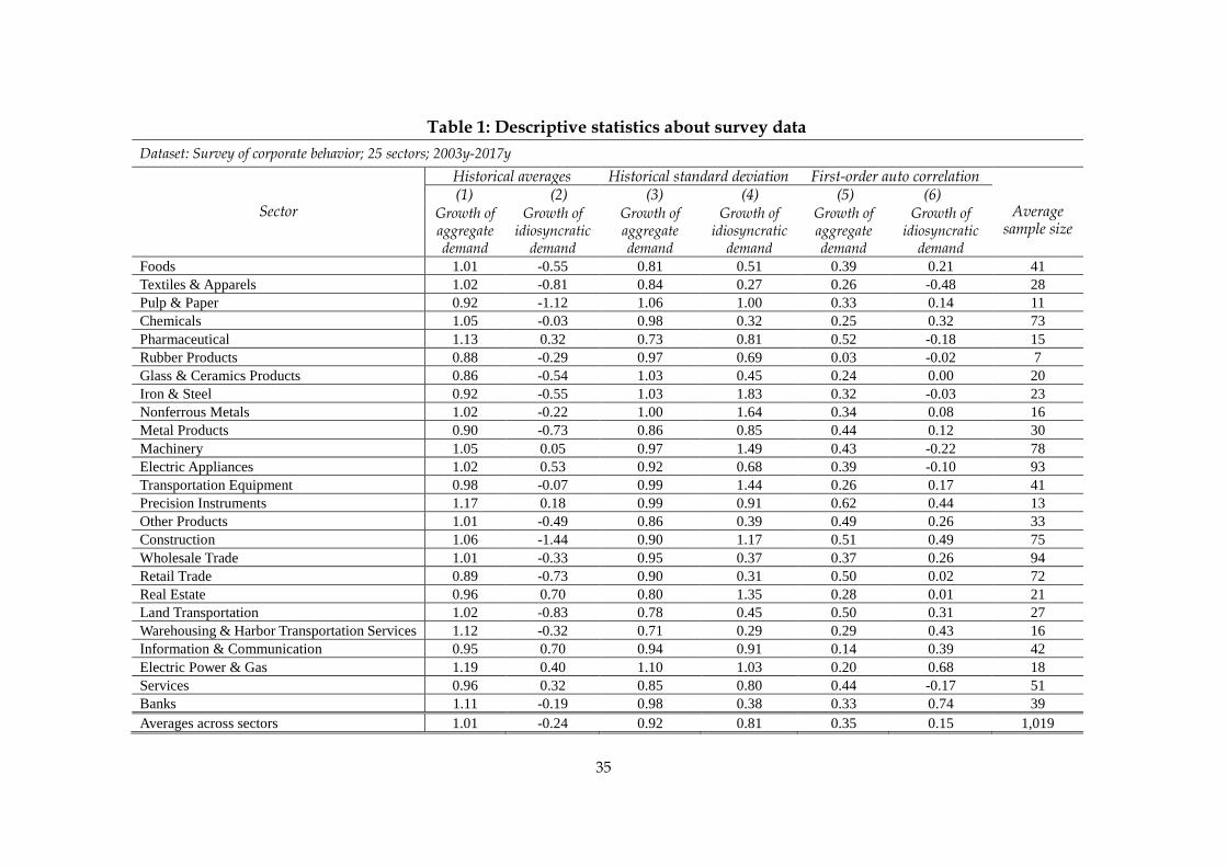
Table 1 provides summary statistics from survey data. Columns (1) and (2) shows histor-
4The industries included in the sample are Foods, Textiles and Apparels, Pulp and Paper, Chemicals,Pharmaceutical, Rubber Products, Glass and Ceramics Products, Iron and Steel, Nonferrous Metals, MetalProducts, Machinery, Electric Appliances, Transportation Equipment, Precision Instruments, Other Prod-ucts, Construction, Wholesale Trade, Retail Trade, Real Estate, Land Transportation, Warehousing andHarbor Transportation Services, Information and Communication, Electric Power and Gas, Services, andBanks. The Economic and Social Research Institute in the Cabinet Office of Japan directly surveys approxi-mately 1,000 public-listed Japanese firms on nominal and real growth rates of the Japanese economy as well asnominal and real growth rates of demand in their respective sectors. Sectoral averages are publicly availableat: http://www.esri.cao.go.jp/en/stat/ank/ank-e.html. The survey is conducted each January, and ques-tionnaires are available at: http://www.esri.cao.go.jp/en/stat/ank/h28ank/h28ank questionnaire.pdf. Weproxy expectations on aggregate demand with survey data on expectations on one-year-ahead GDP growth,and we proxy expectations on sectoral demand with survey data on expectations on one-year-ahead growthrate in sectoral demand.
4

ical averages of the changes in the expectations of one-year-ahead growth rate of aggregate
and idiosyncratic demand, respectively. Entries reveal large differences in the changes of
expectations between the two distinct components of sectoral demand. Changes in the
expectations of aggregate demand are broadly similar across sectors while changes in the
expectations of idiosyncratic demand differ widely across sectors. Columns (3) and (4) show
that both components of sectoral demand have sizeable variation over the sample period and
that the average volatility of the two components is similar.5 Finally, columns (5) and (6)
show that both components have high serial correlation and that the average persistence of
aggregate component is twice as large as the persistence of the idiosyncratic component.
[Table 1 about here.]
Figure 1 provides an illustrative example on firms’ expectations about sectoral demand
partitioned between aggregate and idiosyncratic components for the chemical sector (panel
(a)) and the retail sector (panel (b)). The figures show that expectations of the growth of
sectoral demand (black line) widely vary over the period, becoming negative during 2008
at the time of the global financial crisis. The contribution of aggregate demand (white
bar) and idiosyncratic demand (gray bar) also change over time. Movements in sectoral
expectations are different across sectors, slow-moving in the retail sector and fast-moving in
the chemical sector. On average, changes in the expectations of idiosyncratic demand are of
similar magnitude to those of aggregate demand, consistent with the evidence in Table 1.
Next, we focus on co-movements between expectations of the distinct aggregate and
idiosyncratic components. Table 2 in column (1) shows results from regressing the measure of
firm’s expectations of the growth rate of aggregate demand on the firm’s expectations about
the growth rate of idiosyncratic demand. The regression coefficient is significant, indicating
a positive correlation between changes in the expectations of aggregate and idiosyncratic
demand. Since historical averages of expected growth rates of idiosyncratic demand vary
across sectors while those of aggregate demand are similar across sectors, panel (b) reports
regression estimates that include dummy variables to control for sector-level fixed effects,
and shows that results continue to hold.
[Table 2 about here.]
5Historical standard deviations are computed as the time-series variation in the sector-level aggregateexpectations about the growth of aggregate demand and that of idiosyncratic demand.
5

To summarize, the analysis establishes the following empirical regularities: (i) expecta-
tions about the idiosyncratic component of demand largely vary across sectors, (ii) expec-
tations about both components are largely and equally volatile, and (iii) they positively
co-move.
In the next section, we develop a model that replicates and interprets these findings.
3 Theoretical Framework
The model is based on Angeletos and La’O (2009b) and Mackowiak et al. (2009) and com-
prises monopolistic competitive firms that face a sectoral demand that additively compounds
aggregate and idiosyncratic components. Firms observe sectoral demand and past realiza-
tions of aggregate and idiosyncratic components. However, they cannot observe current
realizations of each distinct component of demand, and therefore need to infer each compo-
nent to maximize revenues. The economy is populated by a representative household and a
continuum of monopolistic competitive firms that produce differentiated goods indexed by
j ∈ [0, 1] in a continuum of sectors indexed by i ∈ [0, 1]. Each representative household
consumes the whole income, and there is no saving in equilibrium. Time is discrete and
indexed by t.
Households. Preferences of the representative household over consumption, Ct, and labor,
Nt, are described by the utility function:∞∑t=0
βt (logCt −Nt) ,
where β ∈ (0, 1) is the discount rate. The household’s aggregate consumption, Ct, and
consumption of goods in sector i, Ct(i), are defined by the CES consumption aggregators:
Ct ≡[∫ 1
0
(Ct(i)Θt(i))η−1η di
] ηη−1
, and Ct(i) ≡[∫ 1
0
(Ct(i, j))η−1η dj
] ηη−1
,
where η > 1 is the elasticity of substitution across sectors, η > 1 is the elasticity of substitu-
tion across goods in the same sector, Ct(i, j) is consumption of good j in sector i, and Θt(i)
is the sector-specific preference shocks.
Firms. Each firm j in sector i (we refer to is as (i, j)) faces the following demand:
Ct(i, j) = Θη−1t (i)
(Pt(i, j)
Pt(i)
)−η (Pt(i)
Pt
)−ηCt, (1)
6

where Pt(i) ≡[∫ 1
0P 1−ηt (i, j)dj
] 11−η
is the sector i price index, Pt ≡[∫ 1
0P 1−ηt (i)Θη−1
t (i)di] 1
1−η
is the aggregate price index, and the idiosyncratic preference shock, Θt(i), acts as an exoge-
nous demand shifter.6
Each firm (i, j) manufactures a single good Y (i, j), according to the production technol-
ogy:
Yt(i, j) = ALεt(i, j), (2)
where A is aggregate productivity and ε ∈ (0, 1) determines the degree of diminishing
marginal returns in production.
Market Clearing. In a symmetric equilibrium, market clearing implies Yt(i, j) = Ct(i, j)
for each firm (i, j), and Yt = Ct for the economy. Aggregate nominal demand, Qt, is given
by the following cash-in-advance constraint:
Qt = PtCt.
In the rest of the analysis, we use lower-case variables to indicate logarithms of the
corresponding upper-case variables (i.e., xt ≡ logXt).
Optimal Price Setting. We first derive the optimal price setting rule with flexible prices,
assuming perfect information about current nominal shocks. During each period t, the firm
(i, j) sets the optimal price as a mark-up over the marginal cost:
pt(i, j) = µ+mct(i, j), (3)
where µ ≡ η/(η− 1) > 0 is the mark-up and mct(i, j) is the nominal marginal cost faced by
firm (i, j). The nominal marginal cost is the difference between the nominal wage, wt, and
the marginal product of labor:
mct(i, j) = wt + (1− ε) lt(i, j)− a− log(ε). (4)
Using the production technology in equation (2), we express labor input as: lt(i, j) =
[yt(i, j)− a]/ε, which we use in equation (4) to rewrite the nominal marginal cost as:
mct(i, j) = wt +1− εε
yt(i, j)−1
εa− log(ε).
6See Appendix A for the derivation of the demand function for each firm (i, j) and price indexes.
7

The optimal labor supply condition for the representative household is:
wt − pt = ct, (5)
and the linearized-version of consumer demand in equation (1) is:
ct(i, j) = −η (pt(i, j)− pt(i))− η (pt(i)− pt) + ct + (η − 1) θt(i), (6)
where the idiosyncratic preference shock, θt(i), follows the AR(1) process:
θt(i) = ρvθt−1(i) + εt(i), (7)
and εt(i) ∼ N (0, (1− ε)−2 (η − 1)−2 τ 2).
We derive the optimal price-setting rule for firm (i, j) by using equations (5), (6), the
equilibrium conditions, yt(i, j) = ct(i, j) and yt = ct, and the cash-in-advance constraint,
yt = qt − pt, which yields:7
pt(i, j) = r1pt(i) + r2pt + (1− r1 − r2)xt(i) + ξ, (8)
where
xt(i) = qt + vt(i), (9)
vt(i) = (1− ε) (η − 1) θt(i), (10)
ξ =ε
ε+ η (1− ε)(µ− 1
εa− log(ε)), (11)
r1 =(η − η) (1− ε)ε+ η (1− ε)
, (12)
r2 =(η − 1) (1− ε)ε+ η (1− ε)
, (13)
and pt =∫ 1
0pt(i)di.
8 Equation (8) shows that the optimal pricing rule for firm (i, j) is
a weighted average of sectoral prices (pt(i)), aggregate prices (pt), and sectoral demand
(xt(i)). The weight between these terms is determined by parameters r1 and r2 that reflect
the degree of strategic complementarity among firms in the same sector and across sectors,
respectively.
Equation (9) shows that sectoral demand (xt(i)) additively combines the aggregate (qt)
and idiosyncratic components (vt(i)), and equation (10) shows that idiosyncratic demand
7Appendix B shows the derivation of the price setting rule.8Appendix C shows the derivation of the index of aggregate prices.
8

depends on the idiosyncratic preference shock θt(i). The parameter ξ, defined in equation
(11), is a linear transformation of the level of aggregate productivity, a, and without loss of
generality, we normalize aggregate productivity such that ξ = 0.
Since firms in the same sector face same marginal costs and access the same information,
pt(i) = pt(i, j) = pt(i, j′) for j 6= j′. Thus, equation (8) reduces to:
pt(i) = rpt + (1− r)xt(i), (14)
where
r ≡ r2
1− r1
=(η − 1) (1− ε)ε+ η (1− ε)
.
Equation (14) shows that the optimal pricing rule for firm (i, j) is a weighted average
of aggregate prices (pt) and sectoral demand (xt(i)). The weights for average prices and
sectoral demand are determined by the parameter r, which similarly to equation (8) reflects
the degree of strategic complementarity between firms in different sectors.9
Information Structure and Shocks. Next, we describe the change in the environment
under imperfect information. Each firm in sector i observes sectoral demand that changes
in response to aggregate demand and idiosyncratic demand, according to xt(i) = qt + vt(i),
as described by equation (9), without observing the distinct aggregate and idiosyncratic
components.10 Aggregate demand follows stochastic process:
qt = qt−1 + ut, (15)
and ut follows the AR(1) process:
ut = ρuut−1 + et, (16)
where 0 ≤ ρu < 1, and et ∼ N (0, σ2). The idiosyncratic component of demand (vt(i)) de-
pends on the idiosyncratic preference shock (θt(i)) described in equation (7). By normalizing
vt(i) = (1− ε) (η − 1) θt(i), the idiosyncratic demand follows the AR(1) process:
vt(i) = ρvvt−1(i) + εt(i), (17)
9Equation (14) shows that if production technology converges to constant returns (i.e., ε → 1), averageprices become less important in the determination of the price for firm i (i.e., r → 0) since the marginalcost converges to the aggregate nominal wage across firms (i.e., mct(i)→ wt) and heterogeneity in the firms’prices decreases. The magnitude of the idiosyncratic shock decreases (i.e., vt(i) → 0) as the productiontechnology converges to constant returns (i.e., ε→ 1). As a result, in the limiting case of a linear productiontechnology (i.e., ε = 1), the optimal pricing rule is pt(i) = qt + ξ.
10Recent study by Chahrour and Ulbricht (2019) shows that imperfect information on idiosyncratic shocksis important for models with imperfect information to generate realistic business cycle statistics.
9

where 0 ≤ ρv < 1, and εt(i) ∼ N (0, τ 2).
The information set of each firm in sector i in period t comprises knowledge on present
realization of sectoral demand and observed past aggregate and idiosyncratic components of
demands (i.e., Ht(i) ≡{{xs(i)}ts=0, {qs, us, vs(i), θs(i), es, εs(i), εs(i)}t−1
s=0
}). To simplify the
notation, we denote Et ≡ E [•|Ht(i)]. The information structure requires inference on the
distinct and unobserved components of aggregate (qt) and idiosyncratic demand (vt(i)) by
using information from the common signal of sectoral demand (i.e., xt(i) = qt + vt(i)) and
knowledge about past realizations of aggregate and idiosyncratic components of demand,
i.e., qt ∼ N (qt−1 + ρuut−1, σ2) and vt(i) ∼ N (ρvvt−1(i), τ 2), respectively.
Mapping the model in the data. The model characterizes the expectations on the level
of sectoral demand whereas the data refer to the expectations on the changes of sectoral
demand. To map the model into empirical measurements, we derive changes in sectoral
demand by taking the first difference of ∆xt(i) = ∆qt + ∆vt(i). To simplify the notation,
we label xt(i) = ∆xt(i), vt(i) = ∆vt(i), and from equation (15) ut = ∆qt. Using equations
(16)-(17), the change in sectoral demand, xt(i), depends on the change in aggregate demand,
ut, and the change in idiosyncratic demand, vt(i):
xt(i) = ut + vt(i). (18)
The formation of expectations. We use the model to study the link between imper-
fect information on the distinct components of sectoral demand and co-movements in the
expectations about these components.
Using equation (18), we derive expectations at time t about sectoral demand in k-period
ahead:
Et
[k∑
h=1
xt+h(i)
]= Et
[k∑
h=1
ut+h
]+ Et
[k∑
h=1
vt+h(i)
]. (19)
We use equation (19) to investigate co-movements in the expectations of future changes
in aggregate and idiosyncratic demand. If firms observe distinct realizations of aggregate
and idiosyncratic components of sectoral demand, such that Et [ut] = ut and Et [vt] = vt,
the expectations on the distinct components of sectoral demand are independent from each
other and therefore uncorrelated. We use this property to link imperfect information on the
current realizations of the distinct components of sectoral demand with co-movements in the
10

expectations of the distinct components, as outlined in the next proposition. To simplify
notation, we denote the unconditional covariance operator with C.
Proposition 1 If sectoral demand compounds singularly unobservable aggregate and id-
iosyncratic components (i.e., xt(i) = ut + vt(i)), the following relationship holds:
C(Et [ut] ,Et [vt]) > 0⇒ C
(Et
[k∑
h=1
ut+h
],Et
[k∑
h=1
vt+h(i)
])> 0
Proof : See Appendix E.1. �
Proposition 1 shows that co-movements in the expectations on current changes in ag-
gregate and idiosyncratic components of sectoral demands are critical for the correlation
between expectations on future changes of these components. The information structure
in our model implies a positive correlation between current realizations of aggregate and
idiosyncratic components, as a result of imperfect information about the realization of each
single component. Since the firm observes a compounded signal of the two components,
they optimally attribute movements in the signal to both components, and thus expecta-
tions about each distinct component of demand positively co-move.
The findings in Proposition 1 enable us to interpret the positive empirical co-movements
in expectations on aggregate and idiosyncratic demand from survey data outlined in section
2. If we use the model to estimate the regression equation in Table 2, it yields:
Et
[k∑
h=1
ut+h
]= β0 + β1Et
[k∑
h=1
vt+h(i)
], (20)
where β0 is the constant term and β1 is the coefficient that establishes the correlation between
changes in aggregate and idiosyncratic demand. The value for β1 is equal to:
β1 =C(Et[∑k
h=1 ut+h
],Et[∑k
h=1 vt+h(i)])
V(Et[∑k
h=1 vt+h(i)]) . (21)
Equation (21) shows that the value for the correlation coefficient β1 depends on the corre-
lation of expectations about future realizations of aggregate and idiosyncratic demand, which
in turn is determined by the expectations on these components in the current period. Propo-
sition 1 shows that imperfect information implies positive correlation in the expectations on
aggregate and idiosyncratic demand at period t, which generates a positive correlation in the
expectations on future values of these components. The regression coefficient β1 is therefore
positive, consistent with the evidence in survey data.
11

4 Shock Heterogeneity and Inflation Dynamics
This section investigates role of shock heterogeneity, represented by the relative volatility of
the idiosyncratic component relative to aggregate component, for the sensitivity of inflation
to sectoral demand.
To link demand to prices, we enrich the model with nominal price rigidities. Under
nominal rigidities, the optimal price-setting rule in equation (14) continues to hold, but with
expectations formed under imperfect information such that:
pt(i) = rEt[pt] + (1− r)Et[qt + vt(i)] = rEt[pt] + (1− r)Et[xt(i)], (22)
where r ≡ (η − 1) (1− ε) / (ε+ η (1− ε)). Equation (22) shows that imperfect information
plays a critical role for the formation of expectations and therefore is important for optimal
price setting in each sector i.
We embed nominal price rigidities, as in Calvo (1983), and we assume that a firm re-
tains the same price with exogenous probability θ ∈ (0, 1) and otherwise changes the price
optimally. The optimal price for firms in sector i, denoted as p∗t (i), depends on expectations
formed at time t on present and future prices, as described by the pricing rule:
p∗t (i) = (1− βθ)∞∑j=0
(βθ)jEt[pt+j(i)]
= (1− βθ)∞∑j=0
(βθ)j [rEt[pt+j] + (1− r)Et[xt+j(i)]] , (23)
where the second equation is derived by substituting the optimal pricing rule in equation
(22). Equation (23) shows that each firm in sector i sets prices as a weighted average of the
firm’s expectations about current and expected future prices whose expectations depend on
the information set at time t.
The Equilibrium Average Price. Equation (23) provides the equilibrium average price
once we derive expectations for prices and sectoral demand. The next proposition charac-
terizes the equilibrium average price.
Proposition 2 (Analytical solution to the equilibrium average price).
The equilibrium average price is given by
p∗t = [θ + (1− θ)a1] pt−1+ (1− θ) a2qt + (1− θ) a3qt−1 + (1− θ) a4ut−1, (24)
12
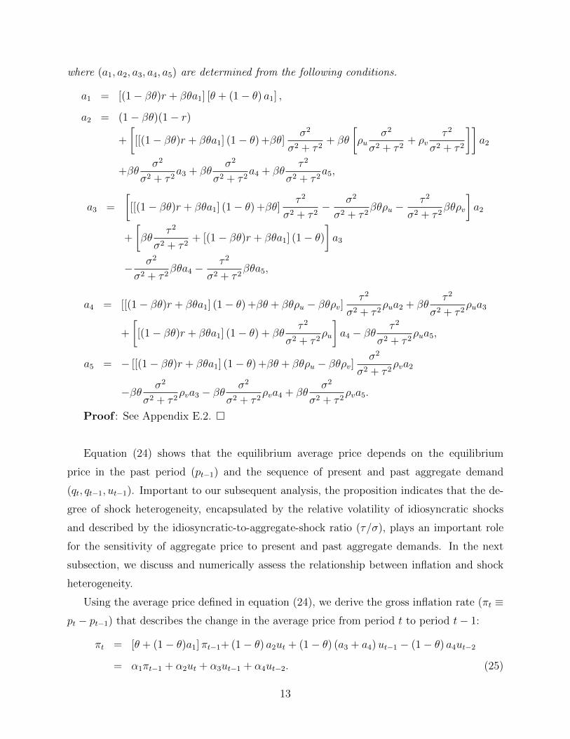
where (a1, a2, a3, a4, a5) are determined from the following conditions.
a1 = [(1− βθ)r + βθa1] [θ + (1− θ) a1] ,
a2 = (1− βθ)(1− r)
+
[[[(1− βθ)r + βθa1] (1− θ) +βθ]
σ2
σ2 + τ 2+ βθ
[ρu
σ2
σ2 + τ 2+ ρv
τ 2
σ2 + τ 2
]]a2
+βθσ2
σ2 + τ 2a3 + βθ
σ2
σ2 + τ 2a4 + βθ
τ 2
σ2 + τ 2a5,
a3 =
[[[(1− βθ)r + βθa1] (1− θ) +βθ]
τ 2
σ2 + τ 2− σ2
σ2 + τ 2βθρu −
τ 2
σ2 + τ 2βθρv
]a2
+
[βθ
τ 2
σ2 + τ 2+ [(1− βθ)r + βθa1] (1− θ)
]a3
− σ2
σ2 + τ 2βθa4 −
τ 2
σ2 + τ 2βθa5,
a4 = [[(1− βθ)r + βθa1] (1− θ) +βθ + βθρu − βθρv]τ 2
σ2 + τ 2ρua2 + βθ
τ 2
σ2 + τ 2ρua3
+
[[(1− βθ)r + βθa1] (1− θ) + βθ
τ 2
σ2 + τ 2ρu
]a4 − βθ
τ 2
σ2 + τ 2ρua5,
a5 = − [[(1− βθ)r + βθa1] (1− θ) +βθ + βθρu − βθρv]σ2
σ2 + τ 2ρva2
−βθ σ2
σ2 + τ 2ρva3 − βθ
σ2
σ2 + τ 2ρva4 + βθ
σ2
σ2 + τ 2ρva5.
Proof : See Appendix E.2. �
Equation (24) shows that the equilibrium average price depends on the equilibrium
price in the past period (pt−1) and the sequence of present and past aggregate demand
(qt, qt−1, ut−1). Important to our subsequent analysis, the proposition indicates that the de-
gree of shock heterogeneity, encapsulated by the relative volatility of idiosyncratic shocks
and described by the idiosyncratic-to-aggregate-shock ratio (τ/σ), plays an important role
for the sensitivity of aggregate price to present and past aggregate demands. In the next
subsection, we discuss and numerically assess the relationship between inflation and shock
heterogeneity.
Using the average price defined in equation (24), we derive the gross inflation rate (πt ≡pt − pt−1) that describes the change in the average price from period t to period t− 1:
πt = [θ + (1− θ)a1] πt−1+ (1− θ) a2ut + (1− θ) (a3 + a4)ut−1 − (1− θ) a4ut−2
= α1πt−1 + α2ut + α3ut−1 + α4ut−2. (25)
13

where α1 ≡ θ + (1− θ)a1, α2 ≡ (1 − θ)a2, α3 ≡ (1 − θ)(a3 + a4), and α4 ≡ −(1 − θ)a4.
Equation (25) is the closed-form solution for inflation under imperfect information. This
formulation is similar to Angeletos and La’O (2009a) since the inflation rate (πt) depends
on past inflation (πt−1) and reacts to current and past changes in demand (ut, and ut−1,
respectively) since demand in the past period t− 1 is fully revealed in the current period t.
Note that α1 = a1 = 0 holds if θ = 0 since nominal price rigidity θ > 0 generates persistence
(i.e., dependence on πt−1). Note also that α3 = a3 = a4 = 0 holds if aggregate price is
perfectly known by firms as τ 2 = 0 and there exists no persistence in aggregate demand
fluctuations (ρu = 0). Under perfect information and flexible prices, the current inflation
rate depends on current changes in aggregate demand.11
4.1 Quantitative Assessment
Using equation (25), we investigate the effect of shock heterogeneity represented by the ratio
of the volatility of the idiosyncratic to aggregate shock (τ/σ) and the degree of nominal
rigidities represented by the parameter θ on the coefficients α1 and α2, which determine the
response of inflation.
Sensitivity of Inflation to Changes in Demand. To study the properties of the system,
we calibrate the model using standard parameter values. We set η = 2, ε = 2/3, r =
[(η − 1)(1 − ε)]/[ε + η(1 − ε)] = 0.5, and β = 0.99. While we estimate the degree of
shock heterogeneity (τ/σ) in the next section to investigate the properties of the model, we
allow the ratio τ/σ to cover a wide range of values [0, 2]. Similarly, we allow the degree of
nominal price rigidity (θ) to cover the whole range of admissible values [0, 1]. The parameters
for the persistence of aggregate and idiosyncratic shocks are set equal to ρu = 0.35 and
ρv = 0.15, respectively, to replicate the average persistence of expectations in aggregate and
idiosyncratic components of demand in survey data.
Panel (a) in Figure 2 shows the sensitivity of parameters α1 and α2 in the closed-form
solution for inflation in equation (25) to the degree of nominal price rigidity (θ). The increase
in nominal price rigidities generates a rise in the coefficient α1 since a low frequency of price
changes increases the importance of past inflation in the determination of current inflation.
11These findings resemble those in Angeletos and La’O (2009a), but they differ across two importantdimensions. First, the coefficients (α2, α3, α4) depend on the volatility of idiosyncratic shocks (τ2), andsecond, inflation depends on the changes in demand two period before ut−2 since aggregate shocks havepositive persistence (ρu > 0).
14

The increase in the degree of nominal price rigidity also generates a decrease in the coefficient
α2 since the sensitivity of individual prices to the current aggregate shock is lowered by less
sensitive average prices, and the sensitivity of average prices to the same shock is directly
dampened by the increase in nominal price rigidity (θ).
Panel (b) in the figure shows that the coefficient α2 depends on the relative volatility
of idiosyncratic shocks (i.e., τ/σ). Individual prices become less sensitive to the current
aggregate shock (α2 decreases). Consequently, the average price becomes less sensitive to
aggregate shocks. Strategic complementarity in the optimal price setting (encapsulated by
r > 0 in equation (14)) induces the firm to largely adjust prices if it perceives the change
in sectoral demand is from the aggregate component, which is common across firms in the
economy. A widening in the volatility of the idiosyncratic component of demand relative to
that of the aggregate component of demand, decreases the response of prices to changes in
sectoral demand. This mechanism explains the negative relationship between τ/σ and α2.
[Figure 2 about here.]
Response of Inflation to Shocks. How does the degree of shock heterogeneity influence
the sensitivity of inflation to changes in demand? To address this important question,
we simulate the model and determine the response of inflation to a one-period, positive
aggregate demand shock. Figure 3 shows that the larger the degree of shock heterogeneity,
as represented by the ratio τ/σ, the lower the response of inflation to changes in current
demand. Since the firm cannot disentangle changes in aggregate and idiosyncratic demand, it
conjectures that changes in sectoral demand are partially caused by changes in idiosyncratic
demand that have no effect on the price-setting decisions of other firms in the economy. This
misperception induces firms to decrease the response to aggregate shocks. If the ratio of τ/σ
is large, the firm conjectures that a large portion of the sectoral demand shock occurs due
to idiosyncratic shock and that aggregate demand does not change. Consequently, the firm
expects that the average price in the period is almost the same as that in the previous period
and adjusts its prices less strongly to changes in demand.
[Figure 3 about here.]
15

4.2 Empirical Assessment
This section first applies principal component analysis to estimate the degree of shock het-
erogeneity. It then applies standard regression analysis to test the relevance of shock het-
erogeneity to the sensitivity of inflation to changes in aggregate demand.
Monte Carlo Experiment. To ensure regression analysis is powerful in detecting the ef-
fect of shock heterogeneity on the sensitivity of inflation to real activity, we conduct a Monte
Carlo experiment. We use the theoretical model as the data-generating process and feed the
system with aggregate shocks, ut, to generate data series for inflation, πt, for 1,000,000 peri-
ods. We allow for different degrees of information heterogeneity, as represented by the ratio,
τ/σ, within the range of values [0, 2] and for degrees of nominal price rigidities, represented
by the parameter θ in the wide range of values {0.2, 0.4, 0.6, 0.8}. To make results consis-
tent with widely used specifications of the Phillips curve, we estimate the slope coefficient
that captures the sensitivity of prices to real activity for two representative versions of the
Phillips curve. First, a New Keynesian Phillips curve that features forward-looking expec-
tations on inflation and second, a hybrid Phillips curve with backward- and forward-looking
expectations on inflation:
πt = βE[πt+1|Ht(i)] + κyt,
πt = (1− γ)E[πt+1|Ht(i)] + κyt + γπt−1,
where the proxy of output gap yt is defined as cumulative changes in output from three
period before yt ≡ yt − yt−3. In our model, Yt = Qt/Pt, and thus yt = (yt − yt−1) +
(yt−1 − yt−2) + (yt−2 − yt−3) = (qt − qt−1) + (qt−1 − qt−2) + (qt−2 − qt−3) − (pt − pt−1) −(pt−1 − pt−2) − (pt−2 − pt−3) = Σ2
j=0 (ut−j − πt−j).12 Panels (a) and (b) in Figure 4 show
estimates for the coefficient κ in the New Keynesian and hybrid Phillips curve, respectively,
for values of τ/σ within the range [0, 1] (on the x-axes) and different degrees of nominal price
rigidity (θ, different lines). For both specifications, the slope coefficient κ is monotonically
decreasing in θ and τ/σ, indicating that the empirical estimation correctly attributes the
increase in information heterogeneity to a reduction in the sensitivity of inflation to real
activity, irrespective of the degree of nominal price rigidity, as predicted by the theoretical
model.12In the estimation, we set β = 0.99 and estimate parameters γ and κ using GMM with lagged inflation.
Although not the main focus of this study, γ changes only slightly along with τ/σ and θ.
16

[Figure 4 about here.]
Estimation of Shock Heterogeneity. We use the Financial Statements Statistics of
Corporations by Industry, compiled by the Ministry of Finance of Japan, which provides
quarterly data on sector-level sales of Japanese firms.13 The data cover the period 1975:Q3-
2018:Q3 for 29 major sectors in the economy. We proxy aggregate shocks by the principal
component of movements in sales growth across sectors. We estimate changes in aggregate
sales, ut, as the principal (first) component of xt(i) across sectors, i ∈ {1, 2, ..., 29}, by
calculating it as ut = Σ29i=1Λixt(i), where Λi is the loading factor of xt(i).
14 We proxy
changes in idiosyncratic demand, vt(i), by subtracting the estimated principal component
from changes in sectoral demand:15 xt(i) − (Σ29i=1Λi)
−1ut = xt(i) − (Σ29
i=1Λi)−1
Σ29i=1Λixt(i),
where the term (Σ29i=1Λi)
−1normalizes ut.
16
We proxy the variance of aggregate fluctuations, 11−ρu2σ
2t with the average of the square
of the extracted principle component for alternative moving windows of size 2k + 1:
1
1− ρu2σ2t =
1
2k + 1Σks=−k
(Σ29i=1Λixt+s(i)
)2. (26)
Similarly, we proxy the variance of the idiosyncratic fluctuations, 11−ρv2 τ
2, with the av-
erage of the square of the proxy of idiosyncratic demand for alternative moving windows of
size 2k + 1:
1
1− ρv2τ 2t =
1
2k + 1Σks=−kΣ
29i=1
[xt+s(i)−
(Σ29i=1Λi
)−1Σ29i=1Λixt+s(i)
]2
. (27)
To ensure robustness of results, we compute the variance of each of the shocks in equations
(26) and (27), using four alternative time windows: two-years (k = 4), three-years (k = 6),
13Specifically, the following sectors are included in our dataset: Foods, Textiles, Wood Products,Pulp and Paper, Printing, Chemicals, Oil and Coal Products, Glass and Ceramics Products, Ironand Steel, Nonferrous Metals, Metal Products, Machinery, Electric Devices, Cars and Related Prod-ucts, Other Transportation Equipment, Other Products, Mining, Construction, Electric Power, Gas andWater Supply, Information and Communication, Land Transportation, Water Transportation, Whole-sale, Retail, Real Estate, Hotel, Living-Related Service, Other Service. The data is available athttp://www.mof.go.jp/english/pri/reference/ssc/index.htm.
14The proportion of the variance of the first component is around 19%, which is considerably larger thanthe variance of the second component (7%), suggesting that the second principal component plays a limitedrole in aggregate shocks.
15To ensure results are robust to alternative normalizations, we implement alternative specifications. First,
we define ut = Σ29i=1Λixt(i) and xt(i)−ut, and second, we define ut =
(Σ29
i=1Λi
)−1Σ29
i=1Λixt(i) and xt(i)−ut.Results remain unchanged across different normalization assumptions.
16Since the proxy for aggregate shock is ut = Σ29i=1Λixt(i) and the sectoral shock is xt(i), the scale
of aggregate shocks Σ29i=1Λi may differ from the scale of sectoral shocks. Estimation results reveal that
Σ29i=1Λi ≈ 4.7, which we use to normalize ut.
17

five-years (k = 10), and ten-years (k = 20). We exclude the upper and lower 10% of
the samples as outliers. Because the dataset shows that persistence of the aggregate and
idiosyncratic fluctuations in each sector does not have time trends, we assume constant
values for the parameters ρu and ρv. The variance of the aggregate component of demand,
11−ρu2σ
2t , and the variance of the idiosyncratic component of demand, 1
1−ρv2 τ2t , are monotonic
with respect to the aggregate shocks σt and τt. By setting to zero the constant terms in the
variances (i.e., 1/(1−ρu2) and 1/(1−ρv2)), we measure shock heterogeneity as the ratio of the
square root of the estimate of the variance of idiosyncratic shocks (τ 2t ) to that of aggregate
shocks for each period (σ2t ). In our specification, the level of τt/σt does not indicate the
absolute level of shock heterogeneity, but it provides a good proxy for the relative variation
in shock heterogeneity.
Panel (a) in Figure 5 shows the estimated series for shock heterogeneity, defined as the
ratio of the variance of idiosyncratic shocks to the variance of aggregate shocks (τt/σt), for
the alternative time windows. Entries show that the degree of information heterogeneity has
steadily increased throughout the sample period, with the ratio τt/σt rising from a value of
2 in the early 1980s to 4 in the mid-2000s, subsequently reaching a value of approximately
3 after 2010 in the 10-year window. Shorter time windows show similar dynamics, despite
increasing volatility. Overall, the analysis detects a robust increase in shock heterogeneity
in the post-2008 period.17
[Figure 5 about here.]
Estimation of the Phillips Curve. In this section, we use the proxy for information
heterogeneity to assess the empirical importance of shock heterogeneity for the reduced
sensitivity of inflation to changes in demand over time.
To implement the estimation of the Phillips curve, we use insights from the theoretical
model in equation (25) that links information frictions to inflation. We regress current infla-
tion on past inflation (πt−1), changes in current aggregate demand (ut), and an interaction
term between changes in current aggregate demand and the degree of shock heterogeneity
(ut × τt/σt) that captures the differential effect of shock heterogeneity for the effect of ag-
gregate demand on current inflation. Following the insights from the theoretical model, we
17Movements in τt/σt are primarily driven by changes in τt since the value for σt remains broadly stableacross the sample period, except during the period of the global financial crisis (2007:4Q to 2010:1Q).Appendix D shows that the aggregate shock series extracted from industry-level data are consistent withmeasures of aggregate shocks as proxied by the output gap.
18

include aggregate demand with two lags.18 Table 3 shows the estimates for the Phillips curve
with measures of shock heterogeneity based on time windows of two years (column (1)), three
years (columns (2)), five years (column (3)) and ten years (column (4)), respectively. All
entries show that current inflation is positively correlated with past inflation and current
demand. This finding is in line with the fundamental prediction of the Phillips curve. The
interaction term is negative, implying that a rise in shock heterogeneity reduces the positive
correlation between inflation and aggregate demand, in accordance with the results of the
analysis, and shows that the raise in shock heterogeneity plays an empirically significant part
in the reduced sensitivity of inflation to real activity.
The theoretical analysis in section 4.1 shows that the degree of nominal price rigidity
is positively related to the flattening of the Phillips curve. To ensure the findings are not
driven by the reduced degree of nominal price rigidity over the sample period, we control
the estimation for the degree of nominal price rigidity by using a dummy variable equal to 1
for the period 2000-2018 when nominal price rigidities decreased (see evidence in Sudo et al.
(2014) and Kurachi et al. (2016)). We also enrich the estimation of the Phillips curve with
two additional interaction terms. The first term interacts the dummy variable for nominal
price rigidities with past inflation (πt−1 × dummy) to capture the interplay between the
degree of nominal price rigidity and the effect of past inflation on current inflation. The
second term interacts the dummy variable for nominal price rigidities with current aggregate
demand (ut× dummy) to capture the interplay between nominal price rigidities and current
aggregate demand. Table 4 reports the results. Columns (1) to (4) show that the coefficient
for the interaction term of past inflation with the dummy variable (πt−1×dummy) is negative,
indicating that the positive correlation between current inflation and past inflation decreases
with a decline in nominal price rigidities, in line with the predictions of our model outlined
in section 4.1. The estimates for the interaction term of changes in demand with the dummy
variable (ut×dummy) are either close to zero and insignificant (columns (1)-(3)) or positive
(columns (2)-(4)), showing that the relationship between inflation and changes in aggregate
demand remains broadly unchanged across periods with different degrees of nominal price
rigidity. This finding corroborates the empirical evidence in Sudo et al. (2014) and Kurachi
et al. (2016), which shows a consistent rise in the frequency of price adjustment across
Japanese firms since the early 2000s. Important for our analysis, the interaction term between
18We also add cross-terms between shock heterogeneity and first-to-second lags of aggregate shocks.
19

aggregate demand and the degree of nominal price rigidity (ut× τt/σt) remains negative and
retains the same magnitude of the benchmark estimates in Table 2, showing that the effect
of the degree of shock heterogeneity is broadly similar across periods with different degrees
of nominal price rigidity.19
[Tables 3 and 4 about here.]
5 Conclusion
We establish novel empirical regularities about expectations of aggregate and idiosyncratic
components of demand using sector-level surveys for the universe of Japanese firms. Expec-
tations of the aggregate component of demand are similar across sectors while expectations
of the idiosyncratic component differ across sectors. Furthermore, expectations of both com-
ponents are largely and equally volatile and they positively co-move.
We develop a theoretical model that links these empirical findings to inflation dynamics.
The model shows a negative relationship between the degree of shock heterogeneity and the
sensitivity of inflation to real activity. We test this theoretical prediction using sector-level
sales data for Japanese firms across 29 sectors, and show that the observed increase in shock
heterogeneity plays a significant role for the reduced sensitivity of inflation to movements in
real activity since the late 1990s.
The analysis opens exiting avenues for additional research. Within the realm of models
with information frictions, an interesting extension would be to endogenize the acquisition of
information, which is likely to interact with the degree of shock heterogeneity in determining
the reaction of aggregate variables to exogenous disturbances, thus playing a potentially im-
portant role for the sensitivity of inflation to aggregate demand. Two promising approaches
to endogenize the information structure are the rational inattention approach (Mackowiak
and Wiederholt, 2009; Mackowiak et al., 2009; and Matejka et al., 2017) and the choice
of information acquisition (Hellwig and Veldkamp, 2009). Another interesting extension is
the study of optimal monetary policy for a comparison with alternative models of imperfect
information (Adam, 2007; Lorenzoni, 2010; Angeletos et al., 2016; and Tamura, 2016). We
will pursue some of these ideas in future work.
19Results continue to hold if we use changes in real aggregate demand. An appendix that details resultsis available from the authors on request.
20

References
Acharya, S. (2017). Costly Information, Planning Complementarities, and the Phillips Curve.Journal of Money, Credit and Banking, 49(4):823–850.
Adam, K. (2007). Optimal monetary policy with imperfect common knowledge. Journal ofMonetary Economics, 54(2):267–301.
Akerlof, G., Dickens, W., and Perry, G. (1996). The macroeconomics of low inflation. Brook-ings Papers on Economic Activity, 27(1):1–76.
Angeletos, G.-M., Iovino, L., and La’O, J. (2016). Real Rigidity, Nominal Rigidity, and theSocial Value of Information. American Economic Review, 106(1):200–227.
Angeletos, G.-M. and La’O, J. (2009a). Incomplete Information, Higher-Order Beliefs andPrice Inertia. Journal of Monetary Economics, 56(S):19–37.
Angeletos, G.-M. and La’O, J. (2009b). Noisy Business Cycles. NBER Working Papers14982, National Bureau of Economic Research, Inc.
Angeletos, G.-M. and Pavan, A. (2007). Efficient use of information and social value ofinformation. Econometrica, 75(4):1103–1142.
Ball, L. and Mazumder, S. (2011). Inflation Dynamics and the Great Recession. EconomicsWorking Paper Archive 580, The Johns Hopkins University, Department of Economics.
Cacciatore, M. and Fiori, G. (2016). The Macroeconomic Effects of Goods and Labor MarletDeregulation. Review of Economic Dynamics, 20:1–24.
Calvo, G. (1983). Staggered prices in a utility-maximizing framework. Journal of MonetaryEconomics, 12(3):383–398.
Chahrour, R. and Ulbricht, R. (2019). Robust predictions for DSGE models with incompleteinformation. Boston College Working Paper Series, Boston College.
Coibion, O. and Gorodnichenko, Y. (2015). Is the Phillips Curve Alive and Well afterAll? Inflation Expectations and the Missing Disinflation. American Economic Journal:Macroeconomics, 7(1):197–232.
Cornand, C. and Heinemann, F. (2018). Monetary Policy Obeying the Taylor PrincipleTurns Prices Into Strategic Substitutes. Rationality and Competition Discussion PaperSeries 90, CRC TRR 190 Rationality and Competition.
Crucini, M. J., Shintani, M., and Takayuki, T. (2015). Noisy information, distance and lawof one price dynamics across US cities. Journal of Monetary Economics, 74(C):52–66.
Dupor, B., Kitamura, T., and Tsuruga, T. (2010). Integrating sticky prices and stickyinformation. The Review of Economics and Statistics, 92(3):657–669.
21

Fukunaga, I. (2007). Imperfect Common Knowledge, Staggered Price Setting, and the Effectsof Monetary Policy. Journal of Money, Credit and Banking, 39(7):1711–1739.
Hellwig, C. and Veldkamp, L. (2009). Knowing What Others Know: Coordination Motivesin Information Acquisition. Review of Economic Studies, 76(1):223–251.
Hellwig, C. and Venkateswaran, V. (2009). Setting the Right Prices for the Wrong Reasons.Journal of Monetary Economics, 56(S):57–77.
IMF (2016). How Has Globalization Affected Inflation? In Fund, I. M., editor, World Eco-nomic Outlook April 2006 Globalization and Inflation, chapter 3. International MonetaryFund.
Kaihatsu, S., Katagiri, M., and Shiraki, N. (2017). Phillips Curve and Price-Change Dis-tribution under Declining Trend Inflation. Bank of Japan Working Paper Series 17-E-5,Bank of Japan.
Kaihatsu, S. and Nakajima, J. (2015). Has Trend Inflation Shifted?: An Empirical Analysiswith a Regime-Switching Model. Bank of Japan Working Paper Series 15-E-3, Bank ofJapan.
Kato, R. and Okuda, T. (2017). Market Concentration and Sectoral Inflation under ImperfectCommon Knowledge. IMES Discussion Paper Series 17-E-11, Institute for Monetary andEconomic Studies, Bank of Japan.
Koga, M., Yoshino, K., and Sakata, T. (2019). Strategic Complementarity and AsymmetricPrice Setting among Firms. Bank of Japan Working Paper Series 19-E-5, Bank of Japan.
Kurachi, Y., Hiraki, K., and Nishioka, S. (2016). Does a Higher Frequency of Micro-levelPrice Changes Matter for Macro Price Stickiness?: Assessing the Impact of TemporaryPrice Changes. Bank of Japan Working Paper Series 16-E-9, Bank of Japan.
L’Huillier, J.-P. (2019). Consumers’ imperfect information and endogenous price rigidities.American Economic Journal: Macroeconomics, Forthcoming.
L’Huillier, J.-P. and Zame, William, R. (2014). The flattening of the phillips curve and thelearning problem of the central bank. Technical report, Einaudi Institute for Economicsand Finance (EIEF).
Lorenzoni, G. (2010). Optimal Monetary Policy with Uncertain Fundamentals and DispersedInformation . Review of Economic Studies, 77(1):305–338.
Lucas, R. (1972). Expectations and the Neutrality of Money. Journal of Economic Theory,4(2):103–124.
Mackowiak, B., Moench, E., and Wiederholt, M. (2009). Sectoral Price Data and Models ofPrice Setting. Journal of Monetary Economics, 56(S):78–99.
Mackowiak, B. and Wiederholt, M. (2009). Optimal Sticky Prices under Rational Inattention.American Economic Review, 99(3):769–803.
22
Mankiw, G. and Reis, R. (2002). Sticky Information versus Sticky Prices: A Proposalto Replace the New Keynesian Phillips Curve. The Quarterly Journal of Economics,117(4):1295–1328.
Matejka, F., Mackowiak, B., and Wiederholt, M. (2017). The Rational Inattention Filter.Working Paper Series 2007, European Central Bank.
Mavroeidis, S., Plagborg-Moller, M., and Stock, J. (2014). Empirical Evidence on Infla-tion Expectations in the New Keynesian Phillips Curve. Journal of Economic Literature,52(1):124–88.
Melosi, L. (2017). Signalling Effects of Monetary Policy. Review of Economic Studies,84(2):853–884.
Mourougane, A. and Ibaragi, H. (2004). Is There a Change in the Trade-Off Between Outputand Inflation at Low or Stable Inflation Rates?: Some Evidence in the Case of Japan.OECD Economics Department Working Papers 379, OECD Publishing.
Nimark, K. (2008). Dynamic Pricing and Imperfect Common Knowledge. Journal of Mon-etary Economics, 55(2):365–382.
Nishizaki, K., Sekine, T., and Ueno, Y. (2014). Chronic Deflation in Japan. Asian EconomicPolicy Review, 9(1):20–39.
Roberts, J. (2004). Monetary Policy and Inflation Dynamics. Finance and Economics Dis-cussion Series 2004-62, Board of Governors of the Federal Reserve System (U.S.).
Sbordone, A. (2008). Globalization and inflation dynamics: the impact of increased compe-tition. Staff Reports 324, Federal Reserve Bank of New York.
Sudo, N., Ueda, K., and Watanabe, K. (2014). Micro price dynamics under Japan’s lostdecades. Asian Economic Policy Review, 9(1):44–64.
Tamura, W. (2016). Optimal Monetary Policy and Transparency under Informational Fric-tions. Journal of Money, Credit and Banking, 48(6):1293–1314.
Thomas, C. and Zanetti, F. (2009). Labor market reform and price stability: An applicationto the Euro Area. Journal of Monetary Economics, 56(6):885–899.
Veirman, E. D. (2007). Which nonlinearity in the Phillips curve? The absence of acceleratingdeflation in Japan. Reserve Bank of New Zealand Discussion Paper Series DP2007/14,Reserve Bank of New Zealand.
Veldkamp, L. and Wolfers, J. (2007). Aggregate shocks or aggregate information? costlyinformation and business cycle comovement. Journal of Monetary Economics, 54:37–55.
Woodford, M. (2003). Imperfect Common Knowledge and the Effects of Monetary Policy.in P. Aghion, R. Frydman, J. Stiglitz, and M. Woodford, eds., knowledge, information,and expectations in modern macroeconomics: In honour of Edmund S. Phelps, Princeton:Princeton University Press.
23

Zanetti, F. (2009). Effects of product and labor market regulation on macroeconomic out-comes. Journal of Macroeconomics, 31(2):320–332.
Zanetti, F. (2011). Labor market institutions and aggregate fluctuations in a search andmatching model. European Economic Review, 55(5):644–658.
24

A Derivation of Demand Functions and Price Indexes
A.1 Demand Functions
A representative household first determines the allocation of consumption across sectors andthen determines that to goods in each sector taking the expenditure level to each sector asgiven.
Define the expenditure level by Zt ≡∫ 1
0Pt(i)Ct(i)di. The Lagrangean is:
L =
[∫ 1
0
(Ct(i)Θt(i))η−1η di
] ηη−1
− λt(∫ 1
0
Pt(i)Ct(i)di− Zt),
and the first-order conditions are:
Ct(i)− 1ηC
1η
t (Θt(i))η−1η = λtPt(i). (28)
Thus, for any two sectors, the following equation holds:
Ct(i) = Ct(j)
(Pt(i)
Pt(j)
)−η (Θt(i)
Θt(j)
)η−1
.
By substituting the equations into the equation for consumption expenditures (Zt ≡∫ 1
0Pt(i)Ct(i)di),
we have ∫ 1
0
Pt(i)
[Ct(j)
(Pt(i)
Pt(j)
)−η (Θt(i)
Θt(j)
)η−1]di = Zt
⇔ Ct(j) = P−ηt (j)Θη−1t (j)Zt
1∫ 1
0P 1−ηt (i)Θη−1
t (i)di. (29)
By substituting the equation: ∫ 1
0
Pt(i)Ct(i)di = Zt = PtCt,
into equation (29), it yields:
Ct(i) = Θη−1t (i)
(Pt(i)
Pt
)−ηCt
P 1−ηt∫ 1
0P 1−ηt (i)Θη−1
t (i)di. (30)
By defining Pt ≡[∫ 1
0P 1−ηt (i)Θη−1
t (i)di] 1
1−η, we can re-write equation (30) as:
Ct(i) = Θη−1t (i)
(Pt(i)
Pt
)−ηCt.
Making the same calculation for Ct(i) =[∫ 1
0(Ct(i, j))
η−1η dj
] ηη−1
, it yields:
Ct(i, j) =
(Pt(i, j)
Pt(i)
)−ηCt(i).
25

By combining these demand functions, we obtain the demand for good (i, j) as follows.
Ct(i, j) = Θη−1t (i)
(Pt(i, j)
Pt(i)
)−η (Pt(i)
Pt
)−ηCt.
A.2 Price Indexes
We show the derivation of aggregate price index Pt ≡[∫ 1
0P 1−ηt (i)Θη−1
t (i)di] 1
1−ηbecause we
can derive sectoral price index Pt(i) ≡[∫ 1
0P 1−ηt (i, j)dj
] 11−η
by exactly the same method.
Recall that λ−1t indicates the price of one unit of utility. From the first-order condition
(28),
Ct(i)− 1ηC
1η
t (Θt(i))η−1η = λtPt(i)
⇔ Ct(i)η−1ηC
1η
t (Θt(i))η−1η = λtCt(i)Pt(i)
⇔∫ 1
0
(Ct(i)
η−1η
(Θt(i))η−1η
)diC
1η
t = λt
∫ 1
0
Ct(i)Pt(i)di
⇔ Ctλ−1t = Z.
We next derive the aggregate price index. From the first-order condition (28),
Ct(i)− 1ηC
1η
t (Θt(i))η−1η = λtPt(i)
⇔ (Ct(i)Θt(i))− 1η C
1η
t Θt(i) = λtPt(i)
⇔ (Ct(i)Θt(i))1η = C
1η
t Θt(i)λ−1t P−1
t (i)
⇔ (Ct(i)Θt(i))η−1η = C
η−1η
t Θη−1t (i)λ1−η
t P 1−ηt (i)
⇔∫ 1
0
(Ct(i)Θt(i))η−1η di = C
η−1η
t λ1−ηt
∫ 1
0
(P 1−ηt (i)Θη−1
t (i))di
⇔ 1 = λ1−ηt
∫ 1
0
(P 1−ηt (i)Θη−1
t (i))di
⇔ λ−1t =
[∫ 1
0
(P 1−ηt (i)Θη−1
t (i))di
] 11−η
.
26

B Derivation of the Price Setting Rule
Frompt(i, j) = µ+mct(i, j),
ct(i, j) = −η (pt(i, j)− pt(i))− η (pt(i)− pt) + ct + (η − 1) θt(i),
and
mct(i, j) = wt +1− εε
yt(i, j)−1
εa− log(ε),
pt(i, j) is given by,
pt(i, j) = µ+mct(i, j) = µ+ yt + pt −1
εa− log(ε)
+1− εε
[−η (pt(i, j)− pt(i))− η (pt(i)− pt) + ct + (η − 1) θt(i)]
= −1− εε
ηpt(i, j) +1− εε
(η − η) pt(i) +
(1 +
1− εε
η
)pt
+(µ− 1
εa− log(ε)) +
(1 +
1− εε
)yt +
1− εε
(η − 1) θt(i)
= −1− εε
ηpt(i, j) +1− εε
(η − η) pt(i) + (µ− 1
εa− log(ε))
+
(1 +
1− εε
)qt +
1− εε
(η − 1) pt +1− εε
(η − 1) θt(i)
=1−εε
(η − η)
1 + 1−εεηpt(i) +
1
1 + 1−εεη
(µ− 1
εa− log(ε))
+1 + 1−ε
ε
1 + 1−εεηqt +
1−εε
(η − 1)
1 + 1−εεηpt +
1−εε
(η − 1)
1 + 1−εεηθt(i)
=(η − η) (1− ε)ε+ η (1− ε)
pt(i) +ε
ε+ η (1− ε)(µ− 1
εa− log(ε))
+1
ε+ η (1− ε)qt +
(1− ε) (η − 1)
ε+ η (1− ε)pt +
(1− ε) (η − 1)
ε+ η (1− ε)θt(i).
C Derivation of the Index of Aggregate Prices
Recall that: Pt ≡[∫ 1
0P 1−ηt (i)Θη−1
t (i)di] 1
1−ηcan be expressed as, Pt =
[∫ 1
0
(Pt(i)Θt(i)
)1−ηdi
] 11−η
=[∫ 1
0
(Pt(i)
)1−ηdi
] 11−η
, where Pt(i) ≡ Pt(i)Θt(i)
. We then define pt ≡∫ 1
0pt(i)di, such that:
pt ≡∫ 1
0
pt(i)di =
∫ 1
0
pt(i)di−∫ 1
0
θt(i)di =
∫ 1
0
pt(i)di,
since θt(i) ∼ N (0, (1− ε)−2 (η − 1)−2 τ 2) and∫ 1
0θt(i)di = 0.
27

D Aggregate Shocks and the Output Gap
To evaluate whether the extracted shock (ut = Σ29i=1Λixt(i)) is a plausible measure of aggre-
gate disturbances that is consistent with alternative measures, we compare the eight-quartersbackward moving averages of the aggregate shocks, 1
8Σ7s=0ut−s,
20 with the output gap pub-lished by the Bank of Japan.21
Figure A examines the relationship between the dynamics of our estimates for aggregateshocks and the output gaps. It shows that the two series are highly correlated, with acorrelation coefficient equal to 0.72, suggesting that our identified measure for the aggregateshock is consistent with alternative measures of aggregate shocks.22
[Figure A about here.]
20Our measure of the aggregate shock is a flow rather than stock concept. By comparing moving averagesof the aggregate shocks (i.e., the averages of flow data) with the output gap (i.e. stock data), we ensure thatour measure is consistent with conventional measures.
21The series is available here. https://www.boj.or.jp/en/research/research data/gap/index.htm/The description of the methodology for the estimation is here
https://www.boj.or.jp/en/research/brp/ron 2017/ron170531a.htm/.22We conduct the same exercise with the eight-quarters backward moving averages of the normalized real
shocks, 18Σ7
s=0
((Σ29
i=1Λi
)−1ut−s − πt−s
), and obtain the broadly same results (a correlation coefficient equal
to 0.65).
28

E Proofs
E.1 Proof of Proposition 1
We divide the proof of Proposition 1 in two parts: part (i) and part (ii).
Part (i) The terms Et[∑k
h=1 ut+h
]and Et
[∑kh=1 vt+h(i)
]are equal to:
Et
[k∑
h=1
ut+h
]=
1− ρuk+1
1− ρuEt [ut] ,
Et
[k∑
h=1
vt+h(i)
]=
1− ρvk+1
1− ρvEt [vt] ,
respectively. It follows that:
C
(Et
[k∑
h=1
ut+h
]Et
[k∑
h=1
vt+h(i)
])=
1− ρuk+1
1− ρu1− ρvk+1
1− ρvC (Et [ut]Et, [vt]) . (31)
From equation (31), co-movements in expectations of k-period ahead aggregate and idiosyn-cratic demand are determined by co-movements in the expectations about current aggregateand idiosyncratic demand, according to:
C
(Et
[k∑
h=1
ut+h
],Et
[k∑
h=1
vt+h(i)
])= 0 if C(Et [ut] ,Et [vt]) = 0
C
(Et
[k∑
h=1
ut+h
],Et
[k∑
h=1
vt+h(i)
])> 0 if C(Et [ut] ,Et [vt]) > 0
C
(Et
[k∑
h=1
ut+h
],Et
[k∑
h=1
vt+h(i)
])< 0 if C(Et [ut] ,Et [vt]) < 0.
Part (i) of the proof outlines the general relationship between the co-movements in theexpectations on distinct components of demand at the present period t and implied co-movements in the expectations on realizations of these components k-period ahead. If ex-pectations of current aggregate and idiosyncratic demand are mutually independent (i.e.,C(Et [ut] ,Et [vt]) = 0), the correlation between expectations of each component k-periodahead also is independent. However, if their correlation at time t is positive (negative), itgenerates a positive (negative) correlation in the expectations of these components.
29

Part (ii) The terms Et [ut] and Et [vt(i)] are equal to:
Et [ut] =τ 2
σ2 + τ 2(qt−1 + ρuut−1) +
σ2
σ2 + τ 2[xt(i)− ρvvt−1(i)]
= ρuut−1 +σ2
σ2 + τ 2[xt(i)− qt−1 − ρuut−1 − ρvvt−1(i)]
= ρuut−1 +σ2
σ2 + τ 2[et + εt(i)]
Et [vt(i)] =σ2
σ2 + τ 2ρvvt−1(i) +
τ 2
σ2 + τ 2[xt(i)− qt−1 − ρuut−1]
= ρvvt−1(i) +τ 2
σ2 + τ 2[xt(i)− qt−1 − ρuut−1 − ρvvt−1(i)]
= ρvvt−1(i) +τ 2
σ2 + τ 2[et + εt(i)] .
Thus, Et [vt] is given by,
Et [vt(i)] = ρvvt−1(i) +τ 2
σ2 + τ 2[et + εt(i)]− vt−1(i)
= (ρv − 1)vt−1(i) +τ 2
σ2 + τ 2[et + εt(i)] .
It follows that:
C(Et [ut] ,Et [vt]) =σ2
σ2 + τ 2
τ 2
σ2 + τ 2V[et + εt(i)] =
σ2τ 2
σ2 + τ 2> 0. (32)
Since equation (32) establishes C(Et [ut] ,Et [vt]) > 0, part (i) proves Proposition 1. �
30

E.2 Proof of Proposition 2
First, we guess that p∗t (i) takes the following form:
p∗t (i) = a1pt−1+a2xt(i) + a3qt−1 + a4ut−1 + a5vt−1(i).
Given the guess, and since only a randomly selected fraction 1− θ of firms adjusts prices inany given period, we infer that the aggregate price level must satisfy:
pt = θpt−1 + (1− θ)∫ 1
0
p∗t (i)di
= [θ + (1− θ) a1] pt−1+ (1− θ) a2qt + (1− θ) a3qt−1 + (1− θ) a4ut−1.
Therefore, p∗t (i) is obtained as:
p∗t (i) = (1− βθ) [(1− r)xt(i) + rEt [pt]] + βθEt[p∗t+1(i)]
= (1− βθ)(1− r)xt(i) + (1− βθ)rEt [pt] + βθEt[p∗t+1(i)]
= (1− βθ)(1− r)xt(i) + (1− βθ)rEt [pt]
+βθEt [a1pt+a2xt+1(i) + a3qt + a4ut + a5vt(i)]
= (1− βθ)(1− r)xt(i) + [(1− βθ)r + βθa1]Et [pt]
+βθa2Et [xt+1(i)] + βθa3Et [qt] + βθa4Et [ut] + βθa5Et [vt(i)]
= (1− βθ)(1− r)xt(i) + [(1− βθ)r + βθa1]Et [pt]
+βθa2Et [qt + ut+1 + vt+1(i)] + βθa3Et [qt] + βθa4Et [ut] + βθa5Et [vt(i)]
= (1− βθ)(1− r)xt(i) + [(1− βθ)r + βθa1]Et [pt]
+βθ (a2 + a3)Et [qt] + βθ (a2ρu + a4)Et [ut] + βθ (a2ρv + a5)Et [vt(i)] .
The term Et [pt] is given by:
Et [pt] = [θ + (1− θ) a1] pt−1 + (1− θ) a2Et [qt] + (1− θ) a3qt−1 + (1− θ) a4ut−1,
which yields:
p∗t (i) = (1− βθ)(1− r)xt(i) + [(1− βθ)r + βθa1] [θ + (1− θ) a1] pt−1
+ [[(1− βθ)r + βθa1] (1− θ) a2+βθ (a2 + a3)]Et [qt]
+ [(1− βθ)r + βθa1] (1− θ) a3qt−1
+ [(1− βθ)r + βθa1] (1− θ) a4ut−1
+βθ (a2ρu + a4)Et [ut] + βθ (a2ρv + a5)Et [vt(i)]
= (1− βθ)(1− r)xt(i) + [(1− βθ)r + βθa1] [θ + (1− θ) a1] pt−1
+ [[[(1− βθ)r + βθa1] (1− θ) a2+βθ (a2 + a3)] + [(1− βθ)r + βθa1] (1− θ) a3] qt−1
+ [[[(1− βθ)r + βθa1] (1− θ) a2+βθ (a2 + a3)] + βθ (a2ρu + a4)]Et [ut]
+βθ (a2ρv + a5)Et [vt(i)]
+ [(1− βθ)r + βθa1] (1− θ) a4ut−1
= (1− βθ)(1− r)xt(i) + [(1− βθ)r + βθa1] [θ + (1− θ) a1] pt−1
+b1qt−1 + b2Et [ut] + b3Et [vt(i)] + b4ut−1.
31

Since
xt(i) = qt−1 + ρuut−1 + et + ρvvt−1(i) + εt(i)
⇔ et = xt(i)− qt−1 − ρuut−1 − ρvvt−1(i)− εt(i),⇔ εt(i) = xt(i)− qt−1 − ρuut−1 − ρvvt−1(i)− et,
The terms Et [ut] and Et [vt(i)] are equal to:
Et [ut] = ρuut−1 + Et [et]
= ρuut−1 +σ2
σ2 + τ 2[xt(i)− qt−1 − ρuut−1 − ρvvt−1(i)]
Et [vt(i)] = ρvvt−1(i) +τ 2
σ2 + τ 2[xt(i)− qt−1 − ρuut−1 − ρvvt−1(i)] .
It follows that:
p∗t (i) = (1− βθ)(1− r)xt(i) + [(1− βθ)r + βθa1] [θ + (1− θ) a1] pt−1
+b1qt−1 + b2Et [ut] + b3Et [vt(i)] + b4ut−1
= (1− βθ)(1− r)xt(i) + [(1− βθ)r + βθa1] [θ + (1− θ) a1] pt−1
+b2ρuut−1 + b2σ2
σ2 + τ 2[xt(i)− qt−1 − ρuut−1 − ρvvt−1(i)]
+b3ρvvt−1(i) + b3τ 2
σ2 + τ 2[xt(i)− qt−1 − ρuut−1 − ρvvt−1(i)]
+b4ut−1 + b1qt−1
= [(1− βθ)r + βθa1] [θ + (1− θ) a1] pt−1
+
[(1− βθ)(1− r) + b2
σ2
σ2 + τ 2+ b3
τ 2
σ2 + τ 2
]xt(i)
+
[b1 − b2
σ2
σ2 + τ 2− b3
τ 2
σ2 + τ 2
]qt−1
+
[b4 + (b2 − b3)
τ 2
σ2 + τ 2ρu
]ut−1 + [b3 − b2]
σ2
σ2 + τ 2ρvvt−1(i),
and thus the equilibrium conditions are:
a1 = [(1− βθ)r + βθa1] [θ + (1− θ) a1] ,
a2 = (1− βθ)(1− r) + b2σ2
σ2 + τ 2+ b3
τ 2
σ2 + τ 2,
a3 = b1 − b2σ2
σ2 + τ 2− b3
τ 2
σ2 + τ 2,
a4 = b4 + (b2 − b3)τ 2
σ2 + τ 2ρu,
a5 = [b3 − b2]σ2
σ2 + τ 2ρv,
32

where
b1 = [[(1− βθ)r + βθa1] (1− θ) a2+βθ (a2 + a3)] + [(1− βθ)r + βθa1] (1− θ) a3,
b2 = [[(1− βθ)r + βθa1] (1− θ) a2+βθ (a2 + a3)] + βθ (a2ρu + a4) ,
b3 = βθ (a2ρv + a5) ,
b4 = [(1− βθ)r + βθa1] (1− θ) a4.
By simplifying the conditions, we obtain:
a1 = [(1− βθ)r + βθa1] [θ + (1− θ) a1] ,
a2 = (1− βθ)(1− r)
+ [[(1− βθ)r + βθa1] (1− θ) a2+βθ (a2 + a3)]σ2
σ2 + τ 2
+βθ (a2ρu + a4)σ2
σ2 + τ 2+ βθ (a2ρv + a5)
τ 2
σ2 + τ 2
= (1− βθ)(1− r)
+
[[[(1− βθ)r + βθa1] (1− θ) +βθ]
σ2
σ2 + τ 2+ βθ
[ρu
σ2
σ2 + τ 2+ ρv
τ 2
σ2 + τ 2
]]a2
+βθσ2
σ2 + τ 2a3 + βθ
σ2
σ2 + τ 2a4 + βθ
τ 2
σ2 + τ 2a5,
a3 = [[(1− βθ)r + βθa1] (1− θ) a2+βθ (a2 + a3)]τ 2
σ2 + τ 2
+ [(1− βθ)r + βθa1] (1− θ) a3 −σ2
σ2 + τ 2βθ (a2ρu + a4)
− τ 2
σ2 + τ 2βθ (a2ρv + a5)
=
[[[(1− βθ)r + βθa1] (1− θ) +βθ]
τ 2
σ2 + τ 2− σ2
σ2 + τ 2βθρu −
τ 2
σ2 + τ 2βθρv
]a2
+
[βθ
τ 2
σ2 + τ 2+ [(1− βθ)r + βθa1] (1− θ)
]a3
− σ2
σ2 + τ 2βθa4 −
τ 2
σ2 + τ 2βθa5,
a4 = [(1− βθ)r + βθa1] (1− θ) a4
+
[[[(1− βθ)r + βθa1] (1− θ) a2+βθ (a2 + a3)]
+βθ (a2ρu + a4)− βθ (a2ρv + a5)
]τ 2
σ2 + τ 2ρu
= [[(1− βθ)r + βθa1] (1− θ) +βθ + βθρu − βθρv]τ 2
σ2 + τ 2ρua2 + βθ
τ 2
σ2 + τ 2ρua3
+
[[(1− βθ)r + βθa1] (1− θ) + βθ
τ 2
σ2 + τ 2ρu
]a4 − βθ
τ 2
σ2 + τ 2ρua5,
33

a5 = −[
[[(1− βθ)r + βθa1] (1− θ) a2+βθ (a2 + a3)]+βθ (a2ρu + a4)− βθ (a2ρv + a5)
]σ2
σ2 + τ 2ρv
= − [[(1− βθ)r + βθa1] (1− θ) +βθ + βθρu − βθρv]σ2
σ2 + τ 2ρva2
−βθ σ2
σ2 + τ 2ρva3 − βθ
σ2
σ2 + τ 2ρva4 + βθ
σ2
σ2 + τ 2ρva5.�
34
35
Table 1: Descriptive statistics about survey data
Dataset: Survey of corporate behavior; 25 sectors; 2003y-2017y
Sector
Historical averages Historical standard deviation First-order auto correlation
Average sample size
(1) (2) (3) (4) (5) (6)Growth of aggregate demand
Growth of idiosyncratic
demand
Growth of aggregate demand
Growth of idiosyncratic
demand
Growth of aggregate demand
Growth of idiosyncratic
demand
Foods 1.01 -0.55 0.81 0.51 0.39 0.21 41
Textiles & Apparels 1.02 -0.81 0.84 0.27 0.26 -0.48 28
Pulp & Paper 0.92 -1.12 1.06 1.00 0.33 0.14 11
Chemicals 1.05 -0.03 0.98 0.32 0.25 0.32 73
Pharmaceutical 1.13 0.32 0.73 0.81 0.52 -0.18 15
Rubber Products 0.88 -0.29 0.97 0.69 0.03 -0.02 7
Glass & Ceramics Products 0.86 -0.54 1.03 0.45 0.24 0.00 20
Iron & Steel 0.92 -0.55 1.03 1.83 0.32 -0.03 23
Nonferrous Metals 1.02 -0.22 1.00 1.64 0.34 0.08 16
Metal Products 0.90 -0.73 0.86 0.85 0.44 0.12 30
Machinery 1.05 0.05 0.97 1.49 0.43 -0.22 78
Electric Appliances 1.02 0.53 0.92 0.68 0.39 -0.10 93
Transportation Equipment 0.98 -0.07 0.99 1.44 0.26 0.17 41
Precision Instruments 1.17 0.18 0.99 0.91 0.62 0.44 13
Other Products 1.01 -0.49 0.86 0.39 0.49 0.26 33
Construction 1.06 -1.44 0.90 1.17 0.51 0.49 75
Wholesale Trade 1.01 -0.33 0.95 0.37 0.37 0.26 94
Retail Trade 0.89 -0.73 0.90 0.31 0.50 0.02 72
Real Estate 0.96 0.70 0.80 1.35 0.28 0.01 21
Land Transportation 1.02 -0.83 0.78 0.45 0.50 0.31 27
Warehousing & Harbor Transportation Services 1.12 -0.32 0.71 0.29 0.29 0.43 16
Information & Communication 0.95 0.70 0.94 0.91 0.14 0.39 42
Electric Power & Gas 1.19 0.40 1.10 1.03 0.20 0.68 18
Services 0.96 0.32 0.85 0.80 0.44 -0.17 51
Banks 1.11 -0.19 0.98 0.38 0.33 0.74 39
Averages across sectors 1.01 -0.24 0.92 0.81 0.35 0.15 1,019

36
Table 2: Firms’ expectations on aggregate and idiosyncratic demands
Dataset: Survey of corporate behavior; 25 sectors; 2003y-2017y
Dependent Variable: firms’ expectations on the growth rate of the aggregate demand
One year ahead expectations
(1) (2)
Pooled OLS model fixed effect model
Constant 1.05*** 1.07***
(0.02) (0.02)
Firms’ expectations on the
growth rate of the
idiosyncratic demand
0.18*** 0.24**
(0.06) (0.08)
Observations 375 375
Adjusted-R2 0.04 0.01
SE 0.88 0.90
Note: Estimated by ordinary-least-squares. The standard errors are HAC estimators. *** Significant at the 1 percent level. ** Significant at the 5 percent level.* Significant at the 10 percent level.

37
Table 3: Estimation of the Phillips curve (part 1)
Dataset: Financial statement statistics of corporations by industry, consumer price index; 29 sectors; 1976/1Q-2018/3Q
Dependent Variable: Inflation rate (�� , core consumer price index, seasonally adjusted, QoQ)
2 years trimmed mean 3 years trimmed mean 5 years trimmed mean 10 years trimmed mean
Constant 0.083** 0.079** 0.078** 0.075***
(0.032) (0.032) (0.033) (0.027)
Lag of inflation (����) 0.613*** 0.610*** 0.518*** 0.443***
(0.103) (0.109) (0.120) (0.110)
Aggregate shocks (��) 0.019** 0.025** 0.045*** 0.065***
(0.008) (0.011) (0.017) (0.020)
Aggregate shocks×shock heterogeneity (�� ×����� ) -0.006** -0.007** -0.013** -0.018***
(0.003) (0.004) (0.005) (0.006)
Observations 171 171 171 171
Adjusted-R2 0.58 0.58 0.61 0.63
SE 0.39 0.40 0.39 0.37
Note: Estimated by ordinary-least-squares. The standard errors are HAC estimators. Aggregate shocks are calculated as the developments in the principal component of 29 sectors. First and second lags of aggregate shocks are included in estimation as control variables. Data extrapolation using the values in the closest periods is applied for the missing values in the estimates of shock heterogeneity. The series for the core consumer price index is “all items, less fresh food (impact of consumption taxes are adjusted)”.
*** Significant at the 1 percent level. ** Significant at the 5 percent level.* Significant at the 10 percent level.

38
Table 4: Estimation of the Phillips curve (part 2) Dataset: Financial statement statistics of corporations by industry, consumer price index; 29 sectors; 1976/1Q-2018/3Q
Dependent Variable: Inflation rate (�� , core consumer price index, seasonally adjusted, QoQ)
2 years trimmed mean 3 years trimmed mean 5 years trimmed mean 10 years trimmed mean
Constant 0.037 0.030 0.032 0.042
(0.037) (0.036) (0.036) (0.033)
Lag of inflation (����) 0.689*** 0.695*** 0.669*** 0.622***
(0.086) (0.088) (0.095) (0.083)
Lag of inflation×time dummy (2000-2017) -0.755** -0.738*** -0.719*** -0.740**
(���� × 1{���������}) (0.168) (0.178) (0.172) (0.158)
Aggregate shocks (��) 0.026** 0.026** 0.040** 0.093***
(0.011) (0.012) (0.018) (0.023)
Aggregate shocks ×time dummy (2000-2017) -0.006 -0.004 0.002 0.019**
(�� × 1{���������}) (0.008) (0.008) (0.008) (0.008)
Aggregate shocks×shock heterogeneity (�� ×����� ) -0.006** -0.007** -0.011** -0.029***
(0.003) (0.004) (0.006) (0.007)
Observations 171 171 171 171
Adjusted-R2 0.66 0.65 0.65 0.68
SE 0.36 0.36 0.36 0.35
Note: Estimated by ordinary-least-squares. The standard errors are HAC estimators. Aggregate shocks are calculated as the developments in the principal component of 29 sectors. First and second lags of aggregate shocks are included in estimation as control variables. Data extrapolation using the values in the closest periods is applied for the missing values in the estimates of shock heterogeneity. The series for the core consumer price index is “all items, less fresh food (impact of consumption taxes are adjusted)”.
*** Significant at the 1 percent level. ** Significant at the 5 percent level.* Significant at the 10 percent level.

39
Figure 1: Firms’ expectations about their sectoral demand, aggregate demand, and idiosyncratic demand
(a) Chemical (b) Retail
-3
-2
-1
0
1
2
3
4
03 04 05 06 07 08 09 10 11 12 13 14 15 16 17
growth of idiosyncratic demand
growth of aggregate demand
growth of sectoral demand
percent
-3
-2
-1
0
1
2
3
4
03 04 05 06 07 08 09 10 11 12 13 14 15 16 17
growth of idiosyncratic demand
growth of aggregate demand
growth of sectoral demand
percent

40
Figure 2: The slope of the Phillips curve
(a) The degree of nominal price rigidity (�) (b) The degree of shock heterogeneity (τ/σ)
Notes: Parameters are �/� = 1, � = 0.5, � = 0.99, �� = 0.35, �� = 0.15 for (a), and � = 0.2 � = 0.5, � = 0.99, �� = 0.35, �� = 0.15 for (b).
0.0
0.1
0.2
0.3
0.4
0.5
0.6
0.7
0.8
0.9
1.0
0.0 0.1 0.2 0.3 0.4 0.5 0.6 0.7 0.8 0.9 1.0
α1 α2
0.0
0.1
0.2
0.3
0.4
0.5
0.6
0.7
0.8
0.9
1.0
0.0 0.2 0.4 0.6 0.8 1.0 1.2 1.4 1.6 1.8 2.0
α1
α2

41
Figure 3: Responses of aggregate inflation to aggregate shocks (Simulation)
Notes: Parameters are � = 0.5, � = 0.5, � = 0.99,�� = 0.35, �� = 0.15.
0.0
0.1
0.2
0.3
0.4
0.5
0.6
-1 0 1 2 3 4 5 6
perfect information (τ/σ=0)
imperfect information (τ/σ=1)
imperfect information (τ/σ=2)
period
percent

42
Figure 4: Estimates for the slope coefficient in the New Keynesian and the hybrid Phillip Curve
(a) Estimates for the slope coefficient (�) in the New Keynesian
Phillips Curve
(b) Estimates for the slope coefficient (�) in the hybrid Phillips
Curve
Notes: Parameters are � = 0.5, � = 0.99,�� = 0.35, �� = 0.15.
-0.2
-0.1
0.0
0.1
0.2
0.3
0.4
0.5
0.6
0.7
0.8
0.0 0.2 0.4 0.6 0.8 1.0 1.2 1.4 1.6 1.8 2.0
θ=0.2
θ=0.4
θ=0.6
θ=0.8
estimates of
0.0
0.1
0.2
0.3
0.4
0.5
0.6
0.7
0.8
0.9
1.0
0.0 0.2 0.4 0.6 0.8 1.0 1.2 1.4 1.6 1.8 2.0
θ=0.2
θ=0.4
θ=0.6
θ=0.8
estimates of

43
Figure 5: Estimates of shock heterogeneity (��/��)
Notes: Upper and lower 10% of the samples are excluded in estimation. Source: Ministry of Finance “Financial statements statistics of corporations by industry”.
0
1
2
3
4
5
6
7
8
1976 81 86 91 96 01 06 11 16
2 years trimmed mean
3 years trimmed mean
5 years trimmed mean
10 years trimmed mean
estimates of τt/σt

44
Figure A: Aggregate shocks and output gap
Sources: Ministry of Finance “Financial statements statistics of corporations by industry”, Bank of Japan “Output Gap and Potential Growth Rate”.
-8
-6
-4
-2
0
2
4
6
-20
-15
-10
-5
0
5
10
15
1983 85 90 95 00 05 10 15
Aggregate shocks(nominal, 8Q backward MA)
Output gap(right scale)
Normalized aggregate shocks(real, 8Q backward MA, right scale)
%
<Correlation with output gap>
・Normalized aggregate shocks(real, 8Q backward MA) :0.65
・Aggregate shocks(nominal, 8Q backward MA) :0.72