impacts of high penetration of pv in distribution grids ... · 2.1.5 storage by storing energy...

eeh power systemslaboratory

Christina Tzanetopoulou

Impacts of high penetration of PV in

distribution grids and mitigation

strategies.

Semester Thesis

Department:EEH – Power Systems Laboratory, ETH Zurich

Examiner:Prof. Dr. Goran Andersson, ETH Zurich

Supervisors:Evangelos Vrettos, ETH Zurich

Olivier Megel, ETH Zurich

Zurich, August 2013

Special acknowledgements to the Foundation of Education and EuropeanCulture for its kind support during the course of my Master studies, part ofwhich is the present Semester Thesis.

ABSTRACT 1

Abstract

Over the last few years renewable energy technologies are getting increasinginterest due to the rising environmental awareness and potential depletion ofconventional energy resources. The most of the renewable energy potentiallies in distributed generation and especially photovoltaics (PV) which aresubsidized quite often by the government for residential installation.

Despite the benefits of high PV penetration, high penetration might leadto several technical issues sourcing from the fact that distribution grids werenot originally designed to carry generation. The focus of the project is tostudy such technical limitations potentially occurring during steady statewhile assuming symmetrical three-phase operation.

The first part of this project is dedicated to the theoretical study ofthese constraints and relevant mitigation strategies. In the second part, wefocus on the mitigation scenarios of storage and conductor upgrading. Anoptimization algorithm is implemented in order to investigate the impacton PV energy yield. The algorithm suggests optimal location and sizing ofbatteries. Finally, an interpretation of the simulation results is presented.

CONTENTS 2

Contents

1 Introduction 3

2 Limitations on PV penetration 32.1 Overvoltage . . . . . . . . . . . . . . . . . . . . . . . . . . . . 4

2.1.1 Power curtailment . . . . . . . . . . . . . . . . . . . . 42.1.2 Upgrading conductor . . . . . . . . . . . . . . . . . . . 52.1.3 Import reactive power . . . . . . . . . . . . . . . . . . 62.1.4 Reduce substation voltage and reduce voltage across

the line . . . . . . . . . . . . . . . . . . . . . . . . . . 62.1.5 Storage . . . . . . . . . . . . . . . . . . . . . . . . . . 7

2.2 Equipment rating and thermal limits . . . . . . . . . . . . . . 72.2.1 Cable thermal limits . . . . . . . . . . . . . . . . . . . 72.2.2 Transformer thermal limits . . . . . . . . . . . . . . . 72.2.3 Circuit breakers’ reverse flow potential . . . . . . . . . 10

3 Implementation 133.1 Low Voltage grid . . . . . . . . . . . . . . . . . . . . . . . . . 133.2 PV generation . . . . . . . . . . . . . . . . . . . . . . . . . . 15

3.2.1 Location . . . . . . . . . . . . . . . . . . . . . . . . . . 163.2.2 Module characteristics and positioning . . . . . . . . . 163.2.3 Inverter characteristics . . . . . . . . . . . . . . . . . . 18

3.3 Transformer thermal model . . . . . . . . . . . . . . . . . . . 183.4 Battery model . . . . . . . . . . . . . . . . . . . . . . . . . . 203.5 Optimization algorithm . . . . . . . . . . . . . . . . . . . . . 22

3.5.1 AC OPF . . . . . . . . . . . . . . . . . . . . . . . . . 223.5.2 Optimization problem . . . . . . . . . . . . . . . . . . 23

4 Simulation results 264.1 Scenarios 1-3: Upgrading the conductor . . . . . . . . . . . . 264.2 Scenarios 4-6: Using storage . . . . . . . . . . . . . . . . . . . 314.3 Transformer . . . . . . . . . . . . . . . . . . . . . . . . . . . . 33

5 Conclusions 37

References 40

1 INTRODUCTION 3

1 Introduction

Over the last years renewable energy technologies are getting increasing in-terest due to the rising environmental awareness and potential depletion ofconventional energy resources. The most of the renewable energy potentiallies in distributed generation, a term which implies the installation of renew-able energy sources to the distribution grid (low voltage grid) thus leadingto reduced congestions and power losses [26], [2]. Specifically photovoltaics(PV) are highly suitable for distributed generation considering that they arerelatively easily installed, they produce no greenhouse gas emissions duringtheir lifetime and their input energy is abundant. These reasons have con-tributed into them being quite often subsidized by the government for retailuse meaning the residential installation supported by many EU countries’government[5].

At the same time, high penetration of PV in a low voltage grid can bethe cause of several technical issues sourcing from the fact that distributiongrids were not originally designed to carry generation. The focus of theproject is to study such technical limitations potentially occurring duringsteady state while assuming symmetrical three-phase operation.

The first part of this project is dedicated to the theoretical study of theseconstraints and relevant mitigation strategies. In the second part, we focuson the mitigation scenarios of storage and conductor upgrading and an opti-mization algorithm is implemented in order to investigate the impact on PVenergy yield. The implementation of an optimization algorithm which con-siders voltage and thermal limits and derives the optimal location and sizingof batteries is the second goal of the project. The algorithm implementedsimulates a variety of scenarios which are based on a benchmark low voltagegrid with high PV penetration located in Affoltern, Zurich. Real life weatherdata are used to derive the photovoltaic generation. A two-well model ofthe lead-acid batteries is used as storage model and a thermal model of atransformer simulates its hot spot temperature. The interpretation of thesimulation results takes place at the third part of the project.

2 Limitations on PV penetration

Despite its huge theoretical potential, photovoltaics’ high penetration is hin-dered by certain technical constraints related to the operation of the electri-cal power system and the ratings of the electrical components [2]. Distribu-tion systems were originally designed to facilitate the flow of power from thegeneration to the consumers through successively decreasing voltage levels.The challenge that distributed generation introduces derives from the oppo-site power flow that it creates, i.e. from the distribution level towards theMV/LV feeder.

2 LIMITATIONS ON PV PENETRATION 4

The problems that can be caused by high penetration of PV in the sys-tem vary from overvoltages and voltage unbalances to power quality, pro-tection and stability issues. Out of all the potential technical issues createddue to the high penetration of PV, the objective of this semester projectis to focus on the technical issues created during the steady state of thedistribution system, while considering symmetrical three-phase operation(three-wire balanced operation).

2.1 Overvoltage

Overvoltage caused by high PV penetration is a very common reason forconstraining the installed capacity of PV. The grid is challenged the mostduring periods of high PV generation and low load where the possibility ofreverse power flow is the highest.

To have a flow of power from the feeder to the customer the voltage atthe feeder is required to be higher than the one at the connection point.Therefore, the voltage in a traditional distribution grid gradually declinesfrom the feeder to the loads.

The voltage at the connection point of PV to the distribution grid isgiven by the formula:

∆V =(PG − PL)R+ (QG −GL)X

V, (1)

where PG, QG are the active and reactive power of the PV in kW, kVArrespectively, V is the voltage at the connection point in V and R, X are theresistance and reactance in Ω between the main station and the connectionpoint [11].

When PVs are connected across the distribution grid, the voltage profilecould enhance when the generation is consumed by the loads. However,when the PV generation is higher than the consumption the reverse powerflow leads to overvoltages which are not acceptable by the regulations, if theyovercome certain limits. As a result, the voltage profile also reverses. Tomitigate this voltage rise, there are several techniques that can be employed.

2.1.1 Power curtailment

Curtailing the output power of PV so as to reach an acceptable voltagelimit, is the first solution that can be implemented. Besides decreasingthe installed capacity, there are many control methods proposed so that thegenerators’ output is actively curtailed, known as Active Power Curtailment(APC).

An example of a droop-based APC method is described in [1]. Thisexample demonstrates the effectiveness of the method but also considers thechallenge of distributing the curtailment among the producers. Constraining


Figure 1: Forward power flow: voltage rise [3]

Figure 2: Reverse power flow: voltage rise [3]

the output would have an impact on the economic and environmental benefitof the scheme. This method is highly recommended when curtailment isexpected to be infrequent [3].

2.1.2 Upgrading conductor

By upgrading the conductor to one with larger diameter, much smaller re-sistance would be achieved while the reactance would slightly differ. Thiswould prevent the overvoltage but changing the conductor is hard to imple-


ment and would lead to economic disadvantage [3].

2.1.3 Import reactive power

Another way to mitigate overvoltage is to properly manipulate reactivepower so as to minimize the numerator of (1). Ideally, this would mean thatreactive power of PX/R should be imported. Considering that LV grids arehighly resistive (high impedance characteristic, i.e. R/X 1 ) this wouldrequire so much reactive power that would lead to an unacceptable powerfactor [4]. In addition, in LV grids this technique would result in increasedpower losses [6].

Shunt impedances are often used as sinkers of reactive power but theyare slow and are not capable to mitigate against the unpredictable variationsof the PV output. Also , given that they are switched on or off, they providelimited controllability [9], [10].

FACTS (Flexible AC Transmission Systems) can also serve as consumersof reactive power but their high cost can be an obstacle [7]. FACTS con-trollers are devices based on power-electronics therefore, they are able pro-vide fast control [9]. Some FACTS controllers provide an output related tothe voltage of the system at their connection point, presenting a difficultyto determining an optimal set point when high PV fluctuation takes place[7].

Inverters on the other hand are not as costly as FACTS and they canbe employed to take advantage of its potential for both leading and laggingpossibility [7]. By changing the power factor on terms of regulating theamount of reactive power absorbed can be achieved an acceptable outcomedespite the fact that voltage in LV grids is more sensitive to active powerchanges than reactive [6], [8]. The ideal amount of Q cannot be supported.

2.1.4 Reduce substation voltage and reduce voltage across theline

In the case of traditional LV grid, in order to mitigate undervoltages thevoltage is kept a little higher than nominal. Given that at a LV grid theopposite phenomenon is observed, reducing the voltage would be a solution[3].

To maintain the voltage under the threshold, on-load tap changers couldbe used. This would enhance the voltage profile but one should make surethat it would not cause undervoltage to other points under any possiblescenario. In addition, on-load tap changers are slow in regard to the PVoutput fluctuation thus, they are not suitable for closely following the PVoutput fluctuation. Plus, frequent tap changing would increase the risk ofmechanical stress on the transformer.

The same challenges are faced when installing an auto-transformer (or


else known as voltage regulator) in order to reset the voltage along the line.Auto-transformers are on-load tap changers with a voltage ratio 1:1 and areused to keep the voltage in one side constant regardless of the voltage changesat the other side thus splitting the system in two parts [3], [9]. Also addingauto-transformers to mitigate overvoltage due to the high penetration ofPV, decreases system reliability [1].

2.1.5 Storage

By storing energy during periods of surplus and using it during periods ofhigh demand, a lot of benefits can be achieved starting from maximum usageof renewable energy and peak shaving. Using storage as a mitigation methodagainst overvoltages, also contributes to mitigating against the stochasticityand the output fluctuation of PV [20]. On the other hand, storage units arecostly [1].

2.2 Equipment rating and thermal limits

Distributed generation can cause an increased power flow in the grid whichmeans increased current thus jeopardizing the thermal limits of the lineand equipment. Besides thermal limits, the reverse flow requirement is notnecessarily supported by all equipment.

2.2.1 Cable thermal limits

The thermal limit of cables depends on the maximum current that theycan support, which is indicated in their specifications. For overhead linesthe temperature of the conductor is influenced by the conductor’s materialproperties, the conductor’s diameter and surface conditions, the conductor’selectrical current and the ambient weather conditions (wind, sun, air)[12].The heat balance equation determines the current that may be carried :

qc + qr = I2r + qs ⇒ I =

√qc + qr − qs

r, (2)

where qc is the heat loss by convection [W/m], qr is the radiated heatloss [W/m], I the conductor’s current [A] and r the conductor’s resistance[Ω/m] .

For underground cables, the internal thermal resistances and the heatproduction by eddy currents in the metal sheets need to be consideredadditionally[11].

2.2.2 Transformer thermal limits

When the output of distributed generation overpasses the local demand, thesurplus power will flow through the transformer to the higher voltage level.Therefore, the reverse power flow capability of transformers is of interest.


The first transformer that the reverse flow will meet is the distributiontransformer. Distribution transformers are characterized in terms of oper-ating voltage and nominal rating. The latter is indicative of the maximumpower that can be transferred between its two sets of terminals. The pri-mary transformer is the next one to be met by the reverse flow. Primarytransformers are characterized by nominal rating and cycling emergency rat-ing which refers to the maximum power that can be handled periodicallyor for short duration. Primary transformers are often installed in pairs andare sized so that they can carry peak demand load without being overloaded[14].

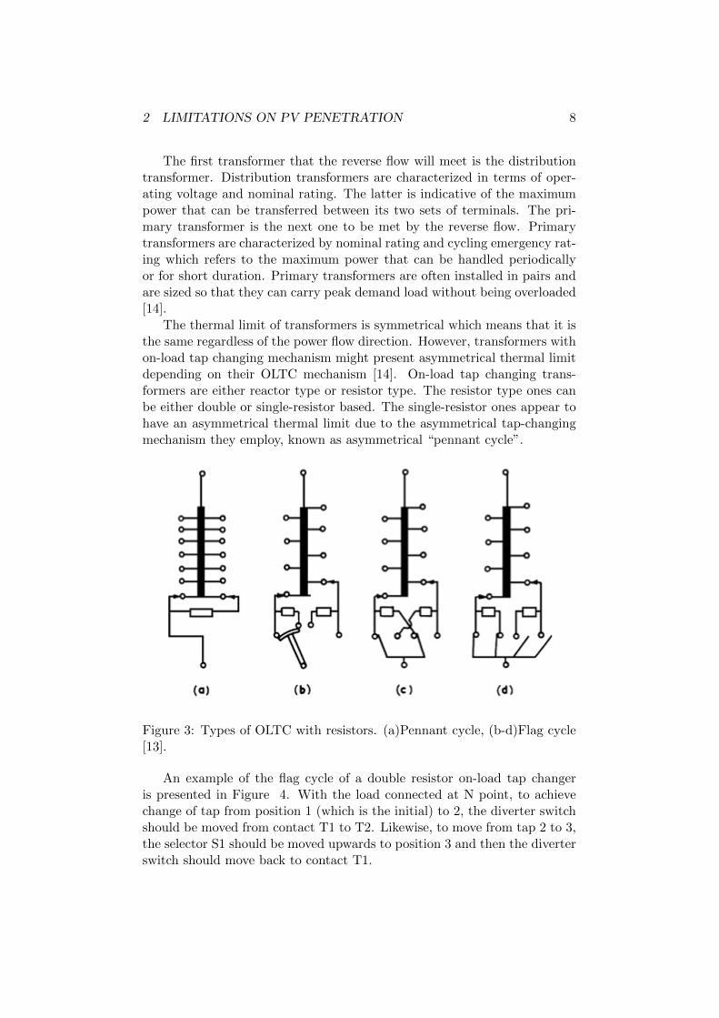
The thermal limit of transformers is symmetrical which means that it isthe same regardless of the power flow direction. However, transformers withon-load tap changing mechanism might present asymmetrical thermal limitdepending on their OLTC mechanism [14]. On-load tap changing trans-formers are either reactor type or resistor type. The resistor type ones canbe either double or single-resistor based. The single-resistor ones appear tohave an asymmetrical thermal limit due to the asymmetrical tap-changingmechanism they employ, known as asymmetrical “pennant cycle”.

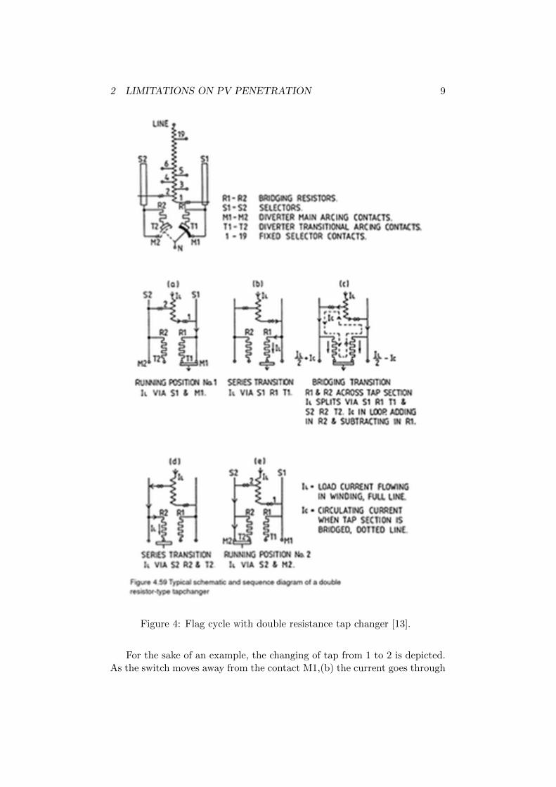
Figure 3: Types of OLTC with resistors. (a)Pennant cycle, (b-d)Flag cycle[13].

An example of the flag cycle of a double resistor on-load tap changeris presented in Figure 4. With the load connected at N point, to achievechange of tap from position 1 (which is the initial) to 2, the diverter switchshould be moved from contact T1 to T2. Likewise, to move from tap 2 to 3,the selector S1 should be moved upwards to position 3 and then the diverterswitch should move back to contact T1.


Figure 4: Flag cycle with double resistance tap changer [13].

For the sake of an example, the changing of tap from 1 to 2 is depicted.As the switch moves away from the contact M1,(b) the current goes through


R1 creating an arc between the moving switch and M1 of voltage equalto the step voltage plus the voltage drop on R1.(c) As the switch meetsR2, a circulating current is created with voltage equal to the step voltagebetween taps 2 and 1, divided by the sum of R1 and R2. (d) Reaching M2,an arc appears between M2 and the moving switch with voltage equal tostep minus the voltage drop on R2. After this analysis, it is clear that areverse power flow which would flow from N towards the transformer wouldimpose the same current switching and recovery voltages but to the alternateside. Therefore, the symmetry of the mechanism results in the most oneroussituation being the same in both cases (in alternate sides) which implies thesame thermal limit regardless of the flow direction [13].

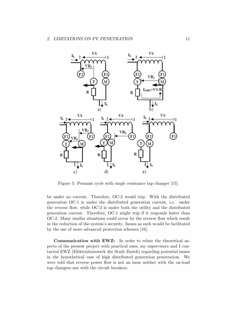
On the other hand, a single-resistor on-load tap changer employs anasymmetrical tap changing mechanism as it can be seen in Figure 5. Tochange tap from position 1 to 2, T moves towards F2 creating a recoveryvoltage VR1= VS (a). When T meets F2, a circulating current occurs equalto VS/R and flow opposite to the load current (b). At the next step, Mmoves away from F1 giving rise to a recovery voltage equal to the stepvoltage minus the voltage drop on the resistance (c). An arc between Tand M occurs when the latter approaches M, under recovery voltage VR4equal to the voltage drop on the resistance. Considering a reverse load flow,one sees that the most onerous situation is related to the fact that M hasto make and break current equal of sum of load current and the circulatingcurrent. However, in case of forward flow the circulating current would besubtracted from the load current. Considering that the thermal limit isdetermined by the most onerous condition of its operation, it is observedthat the asymmetry of the mechanism leads dependency of the limit of theflow direction [15].

2.2.3 Circuit breakers’ reverse flow potential

The reverse connecting or backfeeding possibility of circuit breakers is notclearly investigated in literature. It is suggested that circuit breakers withoutbackfeeding certification should not be used for reverse flow applications.The circuit breakers which can be used for such applications are certified inaccordance to UL489 and UL1066 standards [18],[19].

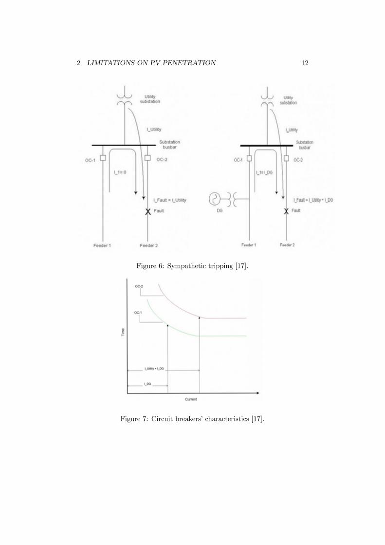
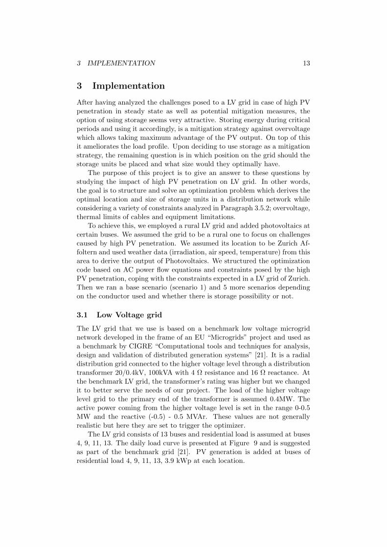
Regardless of the backfeeding potential of circuit breakers, the reversepower flow might cause unnecessary tripping of circuit breakers or miss-coordination of protection elements. An example of such a failure is the“sympathetic tripping”. Sympathetic tripping describes the unnecessarytripping of a circuit breaker due to a fault which takes part on a differentpart of the system [16]. An example can be shown in pictures where a faultin feeder 2 could cause the tripping of the circuit breaker in feeder 1 wheredistributed generation is connected. Without the distributed generation, thecircuit breaker OC-2 would be under the utility current, while OC-1 would


Figure 5: Pennant cycle with single resistance tap changer [15].

be under no current. Therefore, OC-2 would trip. With the distributedgeneration OC-1 is under the distributed generation current, i.e. underthe reverse flow, while OC-2 is under both the utility and the distributedgeneration current. Therefore, OC-1 might trip if it responds faster thanOC-2. Many similar situations could occur by the reverse flow which resultin the reduction of the system’s security. Issues as such would be facilitatedby the use of more advanced protection schemes [16].

Communication with EWZ: In order to relate the theoretical as-pects of the present project with practical ones, my supervisors and I con-tacted EWZ (Elektrizitatswerk der Stadt Zurich) regarding potential issuesin the hypothetical case of high distributed generation penetration. Wewere told that reverse power flow is not an issue neither with the on-loadtap changers nor with the circuit breakers.


Figure 6: Sympathetic tripping [17].

Figure 7: Circuit breakers’ characteristics [17].

3 IMPLEMENTATION 13

3 Implementation

After having analyzed the challenges posed to a LV grid in case of high PVpenetration in steady state as well as potential mitigation measures, theoption of using storage seems very attractive. Storing energy during criticalperiods and using it accordingly, is a mitigation strategy against overvoltagewhich allows taking maximum advantage of the PV output. On top of thisit ameliorates the load profile. Upon deciding to use storage as a mitigationstrategy, the remaining question is in which position on the grid should thestorage units be placed and what size would they optimally have.

The purpose of this project is to give an answer to these questions bystudying the impact of high PV penetration on LV grid. In other words,the goal is to structure and solve an optimization problem which derives theoptimal location and size of storage units in a distribution network whileconsidering a variety of constraints analyzed in Paragraph 3.5.2; overvoltage,thermal limits of cables and equipment limitations.

To achieve this, we employed a rural LV grid and added photovoltaics atcertain buses. We assumed the grid to be a rural one to focus on challengescaused by high PV penetration. We assumed its location to be Zurich Af-foltern and used weather data (irradiation, air speed, temperature) from thisarea to derive the output of Photovoltaics. We structured the optimizationcode based on AC power flow equations and constraints posed by the highPV penetration, coping with the constraints expected in a LV grid of Zurich.Then we ran a base scenario (scenario 1) and 5 more scenarios dependingon the conductor used and whether there is storage possibility or not.

3.1 Low Voltage grid

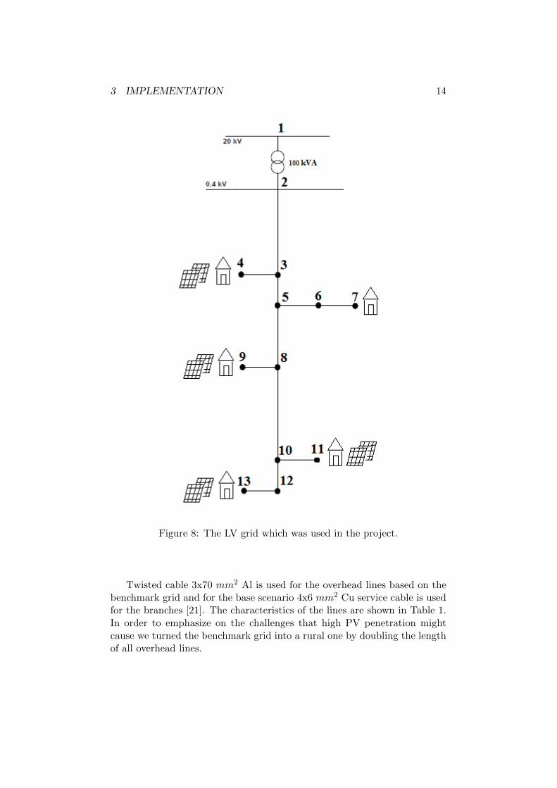
The LV grid that we use is based on a benchmark low voltage microgridnetwork developed in the frame of an EU “Microgrids” project and used asa benchmark by CIGRE “Computational tools and techniques for analysis,design and validation of distributed generation systems” [21]. It is a radialdistribution grid connected to the higher voltage level through a distributiontransformer 20/0.4kV, 100kVA with 4 Ω resistance and 16 Ω reactance. Atthe benchmark LV grid, the transformer’s rating was higher but we changedit to better serve the needs of our project. The load of the higher voltagelevel grid to the primary end of the transformer is assumed 0.4MW. Theactive power coming from the higher voltage level is set in the range 0-0.5MW and the reactive (-0.5) - 0.5 MVAr. These values are not generallyrealistic but here they are set to trigger the optimizer.

The LV grid consists of 13 buses and residential load is assumed at buses4, 9, 11, 13. The daily load curve is presented at Figure 9 and is suggestedas part of the benchmark grid [21]. PV generation is added at buses ofresidential load 4, 9, 11, 13, 3.9 kWp at each location.

3 IMPLEMENTATION 14

Figure 8: The LV grid which was used in the project.

Twisted cable 3x70 mm2 Al is used for the overhead lines based on thebenchmark grid and for the base scenario 4x6 mm2 Cu service cable is usedfor the branches [21]. The characteristics of the lines are shown in Table 1.In order to emphasize on the challenges that high PV penetration mightcause we turned the benchmark grid into a rural one by doubling the lengthof all overhead lines.

3 IMPLEMENTATION 15

00:00 01:00 02:00 03:00 04:00 05:00 06:00 07:00 08:00 09:00 10:00 11:00 12:00 13:00 14:00 15:00 16:00 17:00 18:00 19:00 20:00 21:00 22:00 23:000

0.002

0.004

0.006

0.008

0.01

MW

Daily demand per household: Active Power

00:00 01:00 02:00 03:00 04:00 05:00 06:00 07:00 08:00 09:00 10:00 11:00 12:00 13:00 14:00 15:00 16:00 17:00 18:00 19:00 20:00 21:00 22:00 23:000

0.002

0.004

0.006

0.008

0.01

MV

ar

Daily demand per household: Reactive Power

Figure 9: Daily demand per household.

Branch Line type R (Ω/ km) X (Ω/ km) Length (km) Thermal limit (A)

2 to 3 OL Al 3x70 0.497 0.086 0.07 5703 to 4 SC 4x6 Cu 3.69 0.094 0.03 1353 to 5 OL Al 3x70 0.497 0.086 0.035 5705 to 6 OL Al 3x70 0.497 0.086 0.105 5705 to 8 OL Al 3x70 0.497 0.086 0.105 5707 to 6 SC 4x6 Cu 3.69 0.094 0.03 1358 to 9 SC 4x6 Cu 3.69 0.094 0.03 135

8 to 10 OL Al 3x70 0.497 0.086 0.105 57010 to 12 OL Al 3x70 0.497 0.086 0.35 57011 to 10 SC 4x6 Cu 3.69 0.094 0.03 13512 to 13 SC 4x6 Cu 3.69 0.094 0.03 135

Table 1: Characteristics of the lines of the initial scenario.

3.2 PV generation

To simulate the performance of PV generation we used the PV LIB Toolboxfunctions for Matlab which was developed at Sandia National Laboratories[22]. The data required to derive the PV output were data regarding thegeographical location and series of weather data (radiation, air temperature,wind speed). In addition, the characteristics of the PV modules and theinverter’s are needed as well as details regarding the positioning of modules.

We added photovoltaics of 0.15 MWp, at load buses 4, 9, 11, 13. The

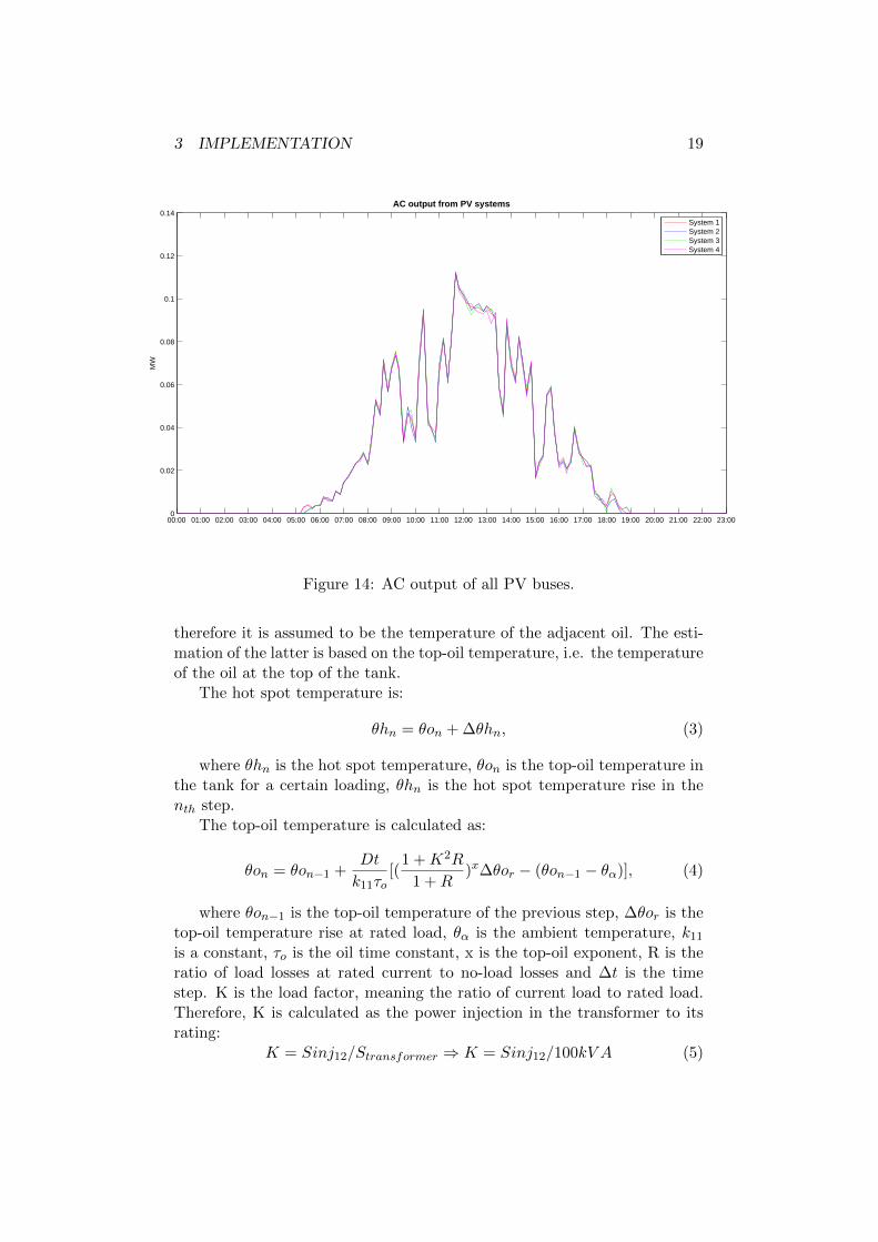
3 IMPLEMENTATION 16

DC and AC output of each generation point is shown in Figures 13, 14.To simulate any possible geographical and/or weather differences from onelocation to another, such as clouds or physical obstacles, we added randomnoise which slightly differentiates the generation from bus to bus.

3.2.1 Location

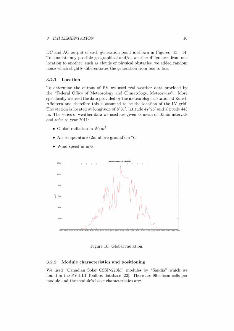
To determine the output of PV we used real weather data provided bythe “Federal Office of Meteorology and Climatology, Meteoswiss”. Morespecifically we used the data provided by the meteorological station at ZurichAffoltern and therefore this is assumed to be the location of the LV grid.The station is located at longitude of 8o31′, latitude 47o26′ and altitude 443m. The series of weather data we used are given as mean of 10min intervalsand refer to year 2011:

• Global radiation in W/m2

• Air temperature (2m above ground) in oC

• Wind speed in m/s

00:00 01:00 02:00 03:00 04:00 05:00 06:00 07:00 08:00 09:00 10:00 11:00 12:00 13:00 14:00 15:00 16:00 17:00 18:00 19:00 20:00 21:00 22:00 23:000

200

400

600

800

1000

1200

W/m

2

Global radiance, 18 July 2011

Figure 10: Global radiation.

3.2.2 Module characteristics and positioning

We used “Canadian Solar CSSP-220M” modules by “Sandia” which wefound in the PV LIB Toolbox database [22]. There are 96 silicon cells permodule and the module’s basic characteristics are:

3 IMPLEMENTATION 17

00:00 01:00 02:00 03:00 04:00 05:00 06:00 07:00 08:00 09:00 10:00 11:00 12:00 13:00 14:00 15:00 16:00 17:00 18:00 19:00 20:00 21:00 22:00 23:008

10

12

14

16

18

20

22o C

Ambient temperature, 18 July 2011

Figure 11: Air temperature.

00:00 01:00 02:00 03:00 04:00 05:00 06:00 07:00 08:00 09:00 10:00 11:00 12:00 13:00 14:00 15:00 16:00 17:00 18:00 19:00 20:00 21:00 22:00 23:000

1

2

3

4

5

6

7

8

m/s

Wind speed, 18 July 2011

Figure 12: Wind speed.

• Power at maximum power point : 217.4 Wp

• Voltage at maximum power point: 48.3 V

• Current at maximum power point: 4.5 A

• Open-circuit voltage: 59.3 V

• Short-circuit current: 5.09 A

3 IMPLEMENTATION 18

The detailed characteristics can be found at http://pvpmc.org/pv-lib/functions-by-catagory/pvl_sapmmoduledb

To achieve maximum PV performance, the positioning of modules playsa very important role. The goal is to take maximum advantage of the solarirradiation. Therefore, we positioned the modules phasing South with anoptimal tilt of 47.4o, i.e. equal to latitude.

3.2.3 Inverter characteristics

To invert the DC output of PV to AC, we used the “BSG5000-U-240Vac”inverter by “Shenzhen Byd Auto” , which we also found in the PV LIB Tool-box database [22]. The inverter’s detailed characteristics can be found at:http://pvpmc.org/pv-lib/functions-by-catagory/pvl_snlinverterdb/

00:00 01:00 02:00 03:00 04:00 05:00 06:00 07:00 08:00 09:00 10:00 11:00 12:00 13:00 14:00 15:00 16:00 17:00 18:00 19:00 20:00 21:00 22:00 23:000

0.02

0.04

0.06

0.08

0.1

0.12

0.14

MW

DC output from PV systems

System 1System 2System 3System 4

Figure 13: DC output of all PV buses.

3.3 Transformer thermal model

To simulate the thermal limit of the transformer, we are calculating the hotspot temperature of the transformer’s windings as indicated in references[24], [25]. After the discussion with EWZ, there was no need to considerthe thermal limit asymmetrical for studying a distribution grid located inZurich. If the transformer is heated above its hot spot temperature, the riskof breaking down the insulating materials is very high. The hot spot tem-perature cannot be directly measured from the temperature of the winding,

http://pvpmc.org/pv-lib/functions-by-catagory/pvl_sapmmoduledb

http://pvpmc.org/pv-lib/functions-by-catagory/pvl_sapmmoduledb

http://pvpmc.org/pv-lib/functions-by-catagory/pvl_snlinverterdb/

3 IMPLEMENTATION 19

00:00 01:00 02:00 03:00 04:00 05:00 06:00 07:00 08:00 09:00 10:00 11:00 12:00 13:00 14:00 15:00 16:00 17:00 18:00 19:00 20:00 21:00 22:00 23:000

0.02

0.04

0.06

0.08

0.1

0.12

0.14

MW

AC output from PV systems

System 1System 2System 3System 4

Figure 14: AC output of all PV buses.

therefore it is assumed to be the temperature of the adjacent oil. The esti-mation of the latter is based on the top-oil temperature, i.e. the temperatureof the oil at the top of the tank.

The hot spot temperature is:

θhn = θon + ∆θhn, (3)

where θhn is the hot spot temperature, θon is the top-oil temperature inthe tank for a certain loading, θhn is the hot spot temperature rise in thenth step.

The top-oil temperature is calculated as:

θon = θon−1 +Dt

k11τo[(

1 +K2R

1 +R)x∆θor − (θon−1 − θα)], (4)

where θon−1 is the top-oil temperature of the previous step, ∆θor is thetop-oil temperature rise at rated load, θα is the ambient temperature, k11

is a constant, τo is the oil time constant, x is the top-oil exponent, R is theratio of load losses at rated current to no-load losses and ∆t is the timestep. K is the load factor, meaning the ratio of current load to rated load.Therefore, K is calculated as the power injection in the transformer to itsrating:

K = Sinj12/Stransformer ⇒ K = Sinj12/100kV A (5)

3 IMPLEMENTATION 20

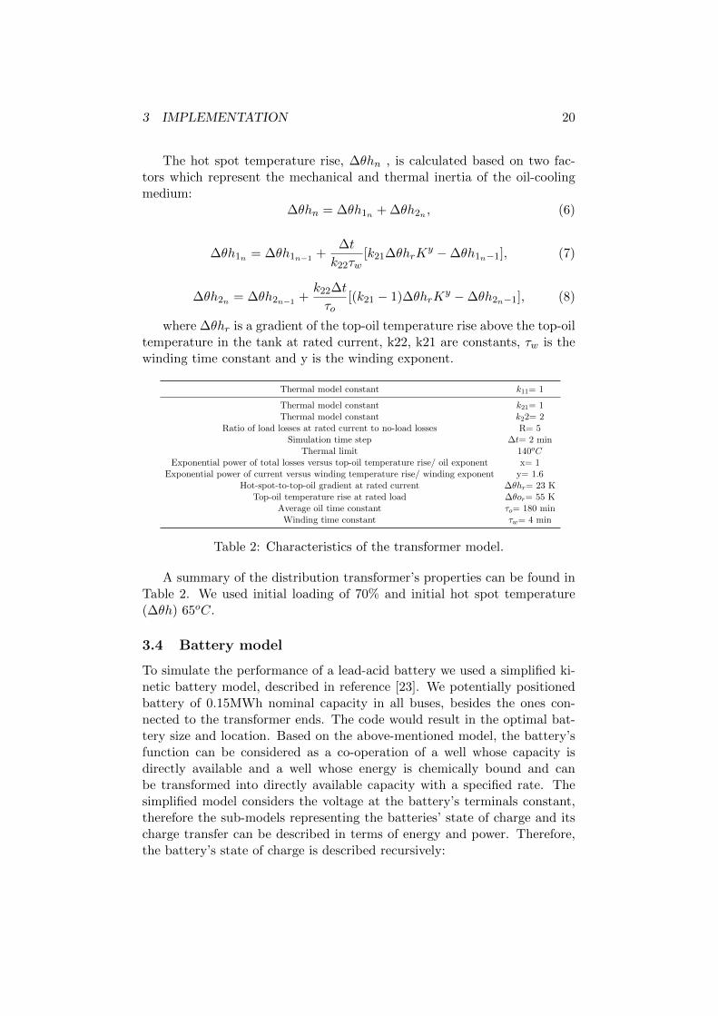
The hot spot temperature rise, ∆θhn , is calculated based on two fac-tors which represent the mechanical and thermal inertia of the oil-coolingmedium:

∆θhn = ∆θh1n + ∆θh2n , (6)

∆θh1n = ∆θh1n−1 +∆t

k22τw[k21∆θhrK

y −∆θh1n−1], (7)

∆θh2n = ∆θh2n−1 +k22∆t

τo[(k21 − 1)∆θhrK

y −∆θh2n−1], (8)

where ∆θhr is a gradient of the top-oil temperature rise above the top-oiltemperature in the tank at rated current, k22, k21 are constants, τw is thewinding time constant and y is the winding exponent.

Thermal model constant k11= 1

Thermal model constant k21= 1Thermal model constant k22= 2

Ratio of load losses at rated current to no-load losses R= 5Simulation time step ∆t= 2 min

Thermal limit 140oCExponential power of total losses versus top-oil temperature rise/ oil exponent x= 1

Exponential power of current versus winding temperature rise/ winding exponent y= 1.6Hot-spot-to-top-oil gradient at rated current ∆θhr= 23 K

Top-oil temperature rise at rated load ∆θor= 55 KAverage oil time constant τo= 180 min

Winding time constant τw= 4 min

Table 2: Characteristics of the transformer model.

A summary of the distribution transformer’s properties can be found inTable 2. We used initial loading of 70% and initial hot spot temperature(∆θh) 65oC.

3.4 Battery model

To simulate the performance of a lead-acid battery we used a simplified ki-netic battery model, described in reference [23]. We potentially positionedbattery of 0.15MWh nominal capacity in all buses, besides the ones con-nected to the transformer ends. The code would result in the optimal bat-tery size and location. Based on the above-mentioned model, the battery’sfunction can be considered as a co-operation of a well whose capacity isdirectly available and a well whose energy is chemically bound and canbe transformed into directly available capacity with a specified rate. Thesimplified model considers the voltage at the battery’s terminals constant,therefore the sub-models representing the batteries’ state of charge and itscharge transfer can be described in terms of energy and power. Therefore,the battery’s state of charge is described recursively:

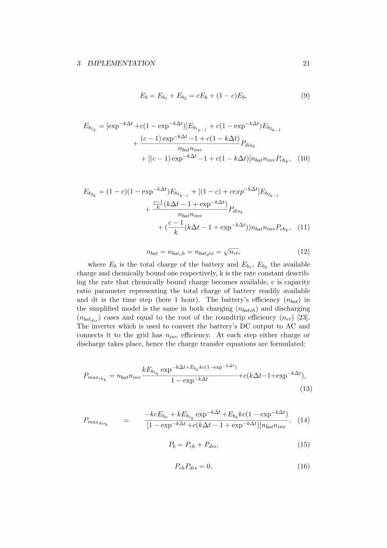
3 IMPLEMENTATION 21

Eb = Eb1 + Eb2 = cEb + (1− c)Eb, (9)

Eb1k = [exp−k∆t +c(1− exp−k∆t)]Eb1k−1+ c(1− exp−k∆t)Eb2k−1

+(c− 1) exp−k∆t−1 + c(1− k∆t)

nbatninvPdisk

+ [(c− 1) exp−k∆t−1 + c(1− k∆t)]nbatninvPchk , (10)

Eb2k = (1− c)(1− exp−k∆t)Eb1k−1+ [(1− c) + cexp−k∆t]Eb2k−1

+c−1k (k∆t− 1 + exp−k∆t)

nbatninvPdisk

+ (c− 1

k(k∆t− 1 + exp−k∆t))nbatninvPchk , (11)

nbat = nbatch = nbatdis =√nrt, (12)

where Eb is the total charge of the battery and Eb1 , Eb2 the availablecharge and chemically bound one respectively, k is the rate constant describ-ing the rate that chemically bound charge becomes available, c is capacityratio parameter representing the total charge of battery readily availableand dt is the time step (here 1 hour). The battery’s efficiency (nbat) inthe simplified model is the same in both charging (nbatch) and discharging(nbatdis) cases and equal to the root of the roundtrip efficiency (nrt) [23].The inverter which is used to convert the battery’s DC output to AC andconnects it to the grid has ninv efficiency. At each step either charge ordischarge takes place, hence the charge transfer equations are formulated:

Pmaxchk = nbatninvkEb1k exp−k∆t+Ebk

kc(1−exp−k∆t)

1− exp−k∆t+c(k∆t−1+exp−k∆t),

(13)

Pmaxdisk =−kcEbn + kEb1k exp−k∆t +Ebkkc(1− exp−k∆t)

[1− exp−k∆t +c(k∆t− 1 + exp−k∆t)]nbatninv, (14)

Pb = Pch + Pdis, (15)

PchPdis = 0, (16)

3 IMPLEMENTATION 22

where Pmaxch and Pmaxdis are the maximum charge and discharge powerat each step and Ebn is the nominal capacity of the battery.The battery’smaximum capacity as well as the constants k and c are available in the bat-tery’s specifications. In the present project we consider batteries’ nominalcapacity to be 0.15MWh each but we assume initial state of charge (SOC)as 20%, i.e. 0.03MWh.

Battery Characteristics

nominal capacity Ebn= 0.15 MWhinitial state of charge 0.03 MWhrate constant k= 1.24capacity ratio c= 0.315round-trip efficiency nrt= 0.86inverter efficiency ninv= 0.92simulation timestep ∆t= 1 hour

Table 3: Characteristics of battery model.

3.5 Optimization algorithm

The optimum location and sizing of the batteries is derived with the helpof an optimization algorithm. The algorithm is calculating the optimumresults within one single day, i.e. 24 hours. This day the algorithm refers to,is the 18th of July 2011 which is calculated as the day with maximum globalradiance within 2011. Therefore, each step of the algorithm represents onereal-life hour. The first step represents the 00:00 - 01:00 interval and so onuntil the 24th step represents the 23:00 - 24:00 interval. To optimize thecoordination between the battery and the PV generation, we use YALMIPwhich is a Matlab toolbox for solving optimization problems, along with theIPOPT solver [27], [28]. YALMIP facilitates the run during the optimiza-tion time horizon in a way that for each timestep the algorithm considers,not only the results of the previous timestep, but the results of the wholeoptimization time horizon.

The optimization runs considering as input the PV generation and theload profile for the day with maximum radiance of the year 2011, 18thof July. The distribution grid structure and specifications as well as thespecifications of the transformer and battery are also considered as input.The algorithm is based on an AC optimal power flow algorithm with theadditions of the transformer and battery models.

3.5.1 AC OPF

The AC power flow algorithm firstly calculates the admittance matrix andthe power injection in the buses. Afterwards, it formulates the power balance

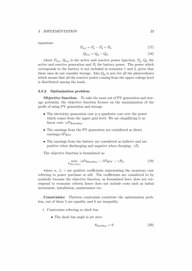
3 IMPLEMENTATION 23

equations:Pinj = Pg − Pd + Pb, (17)

Qinj = Qg −Qd, (18)

where Pinj , Qinj is the active and reactive power injection, Pg, Qg theactive and reactive generation and Pb the battery power. The power whichcorresponds to the battery is not included in scenarios 1 and 2, given thatthese ones do not consider storage. Also Qg is zero for all the photovoltaicswhich means that all the reactive power coming from the upper voltage levelis distributed among the loads.

3.5.2 Optimization problem

Objective function: To take the most out of PV generation and stor-age potential, the objective function focuses on the maximization of theprofit of using PV generation and storage.

• The electricity generation cost is a quadratic cost over the powerwhich comes from the upper grid level. We are simplifying it aslinear cost: αPgslackbus

• The earnings from the PV generation are considered as directearnings:βPgPV

• The earnings from the battery are considered as indirect and arepositive when discharging and negative when charging: γPb

The objective function is formulated as:

minPgslackbus

αPgslackbus − βPgPV − γPb, (19)

where α, β, γ are positive coefficients representing the monetary costreferring to power purchase or sell. The coefficients are considered to bysymbolic because the objective function, as formulated here, does not cor-respond to economic criteria hence does not include costs such as initialinvestment, installation, maintenance etc.

Constraints: Thirteen constraints constitute the optimization prob-lem, out of them 5 are equality and 8 are inequality.

1. Constraints referring to slack bus

• The slack bus angle is set zero:

θslackbus = 0 (20)

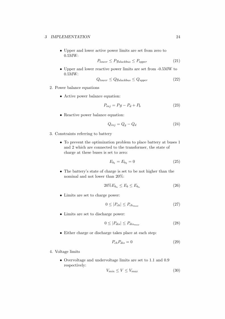
3 IMPLEMENTATION 24

• Upper and lower active power limits are set from zero to0.5MW:

Plower ≤ Pgslackbus ≤ Pupper (21)

• Upper and lower reactive power limits are set from -0.5MW to0.5MW:

Qlower ≤ Qgslackbus ≤ Qupper (22)

2. Power balance equations

• Active power balance equation:

Pinj = Pg − Pd + Pb (23)

• Reactive power balance equation:

Qinj = Qg −Qd (24)

3. Constraints referring to battery

• To prevent the optimization problem to place battery at buses 1and 2 which are connected to the transformer, the state ofcharge at these buses is set to zero:

Eb1 = Eb2 = 0 (25)

• The battery’s state of charge is set to be not higher than thenominal and not lower than 20%:

20%Ebn ≤ Eb ≤ Ebn (26)

• Limits are set to charge power:

0 ≤ |Pch| ≤ Pchmax (27)

• Limits are set to discharge power:

0 ≤ |Pdis| ≤ Pdismax (28)

• Either charge or discharge takes place at each step:

PchPdis = 0 (29)

4. Voltage limits

• Overvoltage and undervoltage limits are set to 1.1 and 0.9respectively:

Vmin ≤ V ≤ Vmax (30)

3 IMPLEMENTATION 25

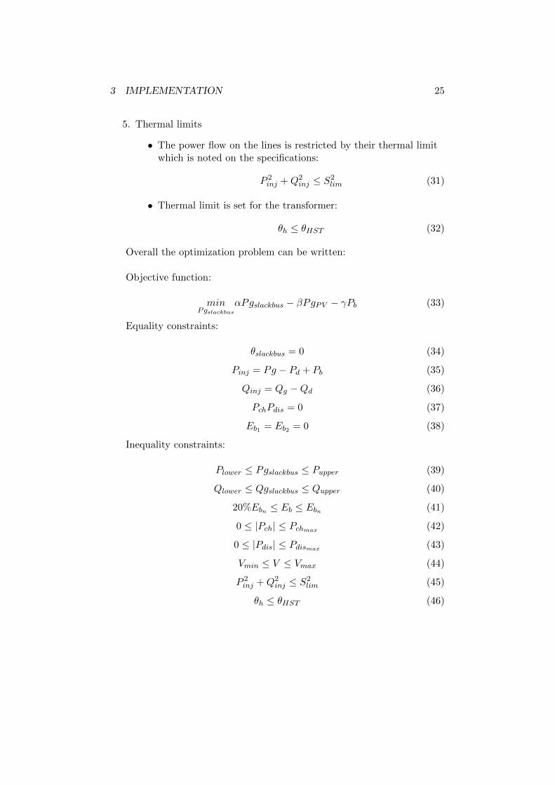
5. Thermal limits

• The power flow on the lines is restricted by their thermal limitwhich is noted on the specifications:

P 2inj +Q2

inj ≤ S2lim (31)

• Thermal limit is set for the transformer:

θh ≤ θHST (32)

Overall the optimization problem can be written:

Objective function:

minPgslackbus

αPgslackbus − βPgPV − γPb (33)

Equality constraints:

θslackbus = 0 (34)

Pinj = Pg − Pd + Pb (35)

Qinj = Qg −Qd (36)

PchPdis = 0 (37)

Eb1 = Eb2 = 0 (38)

Inequality constraints:

Plower ≤ Pgslackbus ≤ Pupper (39)

Qlower ≤ Qgslackbus ≤ Qupper (40)

20%Ebn ≤ Eb ≤ Ebn (41)

0 ≤ |Pch| ≤ Pchmax (42)

0 ≤ |Pdis| ≤ Pdismax (43)

Vmin ≤ V ≤ Vmax (44)

P 2inj +Q2

inj ≤ S2lim (45)

θh ≤ θHST (46)

4 SIMULATION RESULTS 26

4 Simulation results

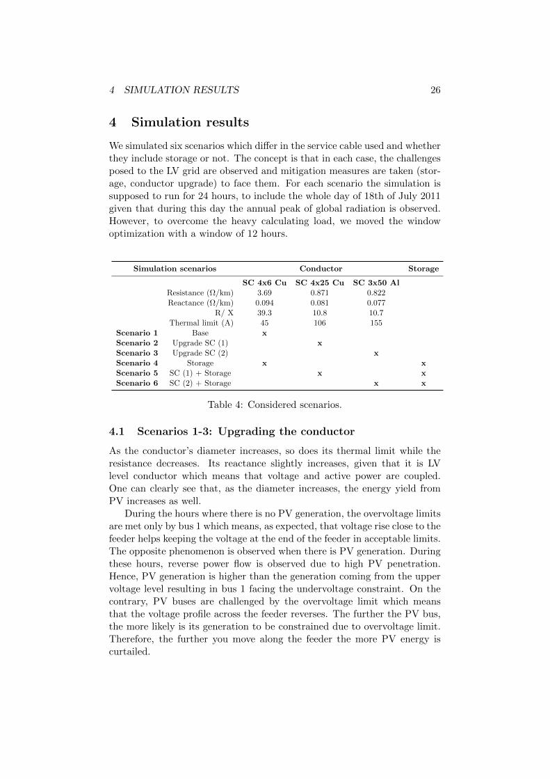
We simulated six scenarios which differ in the service cable used and whetherthey include storage or not. The concept is that in each case, the challengesposed to the LV grid are observed and mitigation measures are taken (stor-age, conductor upgrade) to face them. For each scenario the simulation issupposed to run for 24 hours, to include the whole day of 18th of July 2011given that during this day the annual peak of global radiation is observed.However, to overcome the heavy calculating load, we moved the windowoptimization with a window of 12 hours.

Simulation scenarios Conductor Storage

SC 4x6 Cu SC 4x25 Cu SC 3x50 AlResistance (Ω/km) 3.69 0.871 0.822Reactance (Ω/km) 0.094 0.081 0.077

R/ X 39.3 10.8 10.7Thermal limit (A) 45 106 155

Scenario 1 Base xScenario 2 Upgrade SC (1) xScenario 3 Upgrade SC (2) xScenario 4 Storage x xScenario 5 SC (1) + Storage x xScenario 6 SC (2) + Storage x x

Table 4: Considered scenarios.

4.1 Scenarios 1-3: Upgrading the conductor

As the conductor’s diameter increases, so does its thermal limit while theresistance decreases. Its reactance slightly increases, given that it is LVlevel conductor which means that voltage and active power are coupled.One can clearly see that, as the diameter increases, the energy yield fromPV increases as well.

During the hours where there is no PV generation, the overvoltage limitsare met only by bus 1 which means, as expected, that voltage rise close to thefeeder helps keeping the voltage at the end of the feeder in acceptable limits.The opposite phenomenon is observed when there is PV generation. Duringthese hours, reverse power flow is observed due to high PV penetration.Hence, PV generation is higher than the generation coming from the uppervoltage level resulting in bus 1 facing the undervoltage constraint. On thecontrary, PV buses are challenged by the overvoltage limit which meansthat the voltage profile across the feeder reverses. The further the PV bus,the more likely is its generation to be constrained due to overvoltage limit.Therefore, the further you move along the feeder the more PV energy iscurtailed.


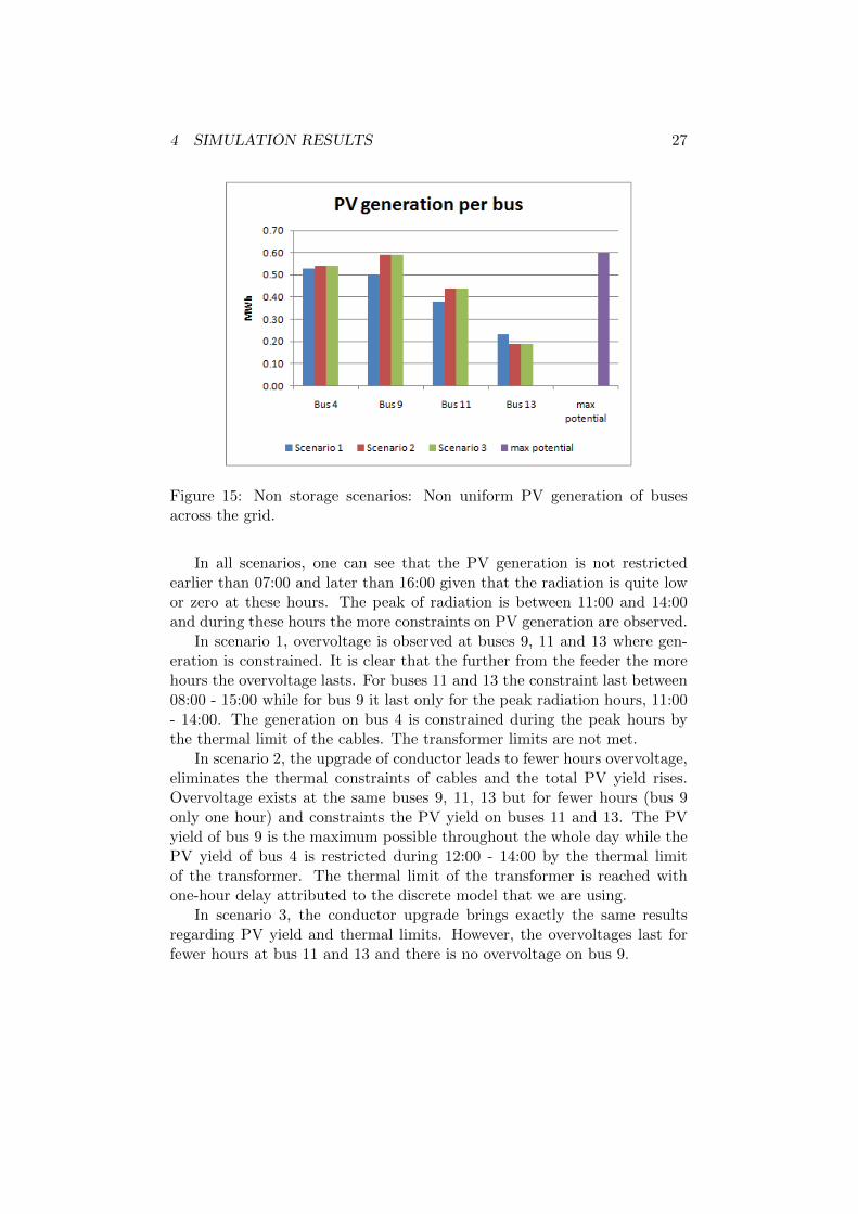
Figure 15: Non storage scenarios: Non uniform PV generation of busesacross the grid.

In all scenarios, one can see that the PV generation is not restrictedearlier than 07:00 and later than 16:00 given that the radiation is quite lowor zero at these hours. The peak of radiation is between 11:00 and 14:00and during these hours the more constraints on PV generation are observed.

In scenario 1, overvoltage is observed at buses 9, 11 and 13 where gen-eration is constrained. It is clear that the further from the feeder the morehours the overvoltage lasts. For buses 11 and 13 the constraint last between08:00 - 15:00 while for bus 9 it last only for the peak radiation hours, 11:00- 14:00. The generation on bus 4 is constrained during the peak hours bythe thermal limit of the cables. The transformer limits are not met.

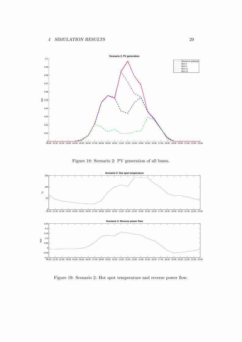
In scenario 2, the upgrade of conductor leads to fewer hours overvoltage,eliminates the thermal constraints of cables and the total PV yield rises.Overvoltage exists at the same buses 9, 11, 13 but for fewer hours (bus 9only one hour) and constraints the PV yield on buses 11 and 13. The PVyield of bus 9 is the maximum possible throughout the whole day while thePV yield of bus 4 is restricted during 12:00 - 14:00 by the thermal limitof the transformer. The thermal limit of the transformer is reached withone-hour delay attributed to the discrete model that we are using.

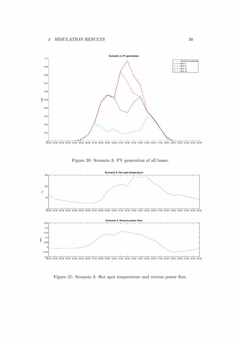
In scenario 3, the conductor upgrade brings exactly the same resultsregarding PV yield and thermal limits. However, the overvoltages last forfewer hours at bus 11 and 13 and there is no overvoltage on bus 9.


00:00 01:00 02:00 03:00 04:00 05:00 06:00 07:00 08:00 09:00 10:00 11:00 12:00 13:00 14:00 15:00 16:00 17:00 18:00 19:00 20:00 21:00 22:00 23:000

0.01

0.02

0.03

0.04

0.05

0.06

0.07

0.08

0.09

0.1

MW

Scenario 1, PV generation

Maximum potentialBus 4Bus 9Bus 11Bus 13

Figure 16: Scenario 1: PV generation of all buses.

00:00 01:00 02:00 03:00 04:00 05:00 06:00 07:00 08:00 09:00 10:00 11:00 12:00 13:00 14:00 15:00 16:00 17:00 18:00 19:00 20:00 21:00 22:00 23:0020

40

60

80

100

120

o C

Scenario 1: Hot spot temperature

00:00 01:00 02:00 03:00 04:00 05:00 06:00 07:00 08:00 09:00 10:00 11:00 12:00 13:00 14:00 15:00 16:00 17:00 18:00 19:00 20:00 21:00 22:00 23:00−0.1

−0.05

0

0.05

0.1

0.15

MW

Scenario 1: Reverse power flow

Figure 17: Scenario 1: Hot spot temperature and reverse power flow.


00:00 01:00 02:00 03:00 04:00 05:00 06:00 07:00 08:00 09:00 10:00 11:00 12:00 13:00 14:00 15:00 16:00 17:00 18:00 19:00 20:00 21:00 22:00 23:000

0.01

0.02

0.03

0.04

0.05

0.06

0.07

0.08

0.09

0.1

MW




00:00 01:00 02:00 03:00 04:00 05:00 06:00 07:00 08:00 09:00 10:00 11:00 12:00 13:00 14:00 15:00 16:00 17:00 18:00 19:00 20:00 21:00 22:00 23:000

50

100

150

o C


00:00 01:00 02:00 03:00 04:00 05:00 06:00 07:00 08:00 09:00 10:00 11:00 12:00 13:00 14:00 15:00 16:00 17:00 18:00 19:00 20:00 21:00 22:00 23:00−0.1

−0.05

0

0.05

0.1

0.15

0.2

0.25

MW




4.2 Scenarios 4-6: Using storage

Adding storage allows taking higher advantage of PV generation. It is clearthat as the conductor diameter increases, the PV yield is higher and theovervoltages are lasting fewer hours. It is also clear that in each scenario,the PV yield decreases as moving away from the feeder while the oppositeapplies to the voltage profile.

Figure 22: Storage scenarios: Non uniform PV generation of buses acrossthe grid.

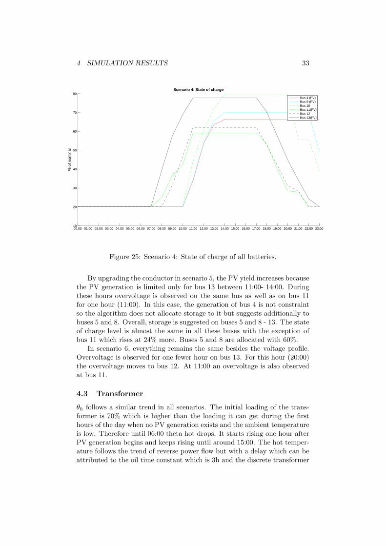
In scenario 4, the PV generation is constrained on bus 11 and 13 duringthe peak hours, 12:00 - 14:00 and 11:00 - 15:00 respectively due to overvolt-age limits. The generation of buses 4 and 9 is limited only for one hour(12:00) due to the thermal limit of the lines and overvoltage respectively.The increased PV yield is permitted thanks to the storage in relation toScenario 1. Batteries are suggested by the algorithm on buses 4 and 9-13. The batteries are charging from 08:00 until 15:00 and discharging from17:00. At the beginning only the batteries located at the lower part of thegrid, there where PV generation was initially restricted, are charging. Astime goes by, batteries are suggested to more and more buses closer to thefeeder. The maximum state of charge for the PV buses 9-13 is on the rangeof 70-85% and 56% for bus 4. The allocation of batteries and their siz-ing is meant to facilitate the voltage profile during their discharging period(in time-horizon and across the feeder). Also the losses over the cables arelower as the voltage is higher meaning that locating batteries on buses withovervoltage is beneficiary. The limits of the transformer are not met.


00:00 01:00 02:00 03:00 04:00 05:00 06:00 07:00 08:00 09:00 10:00 11:00 12:00 13:00 14:00 15:00 16:00 17:00 18:00 19:00 20:00 21:00 22:00 23:000

0.01

0.02

0.03

0.04

0.05

0.06

0.07

0.08

0.09

0.1

MW




00:00 01:00 02:00 03:00 04:00 05:00 06:00 07:00 08:00 09:00 10:00 11:00 12:00 13:00 14:00 15:00 16:00 17:00 18:00 19:00 20:00 21:00 22:00 23:0020

40

60

80

100

120

o C


00:00 01:00 02:00 03:00 04:00 05:00 06:00 07:00 08:00 09:00 10:00 11:00 12:00 13:00 14:00 15:00 16:00 17:00 18:00 19:00 20:00 21:00 22:00 23:00−0.02

0

0.02

0.04

0.06

0.08

0.1

0.12

0.14

MW




00:00 01:00 02:00 03:00 04:00 05:00 06:00 07:00 08:00 09:00 10:00 11:00 12:00 13:00 14:00 15:00 16:00 17:00 18:00 19:00 20:00 21:00 22:00 23:0010

20

30

40

50

60

70

80

% o

f nom

inal

Scenario 4: State of charge

Bus 4 (PV)Bus 9 (PV)Bus 10Bus 11(PV)Bus 12Bus 13(PV)

Figure 25: Scenario 4: State of charge of all batteries.

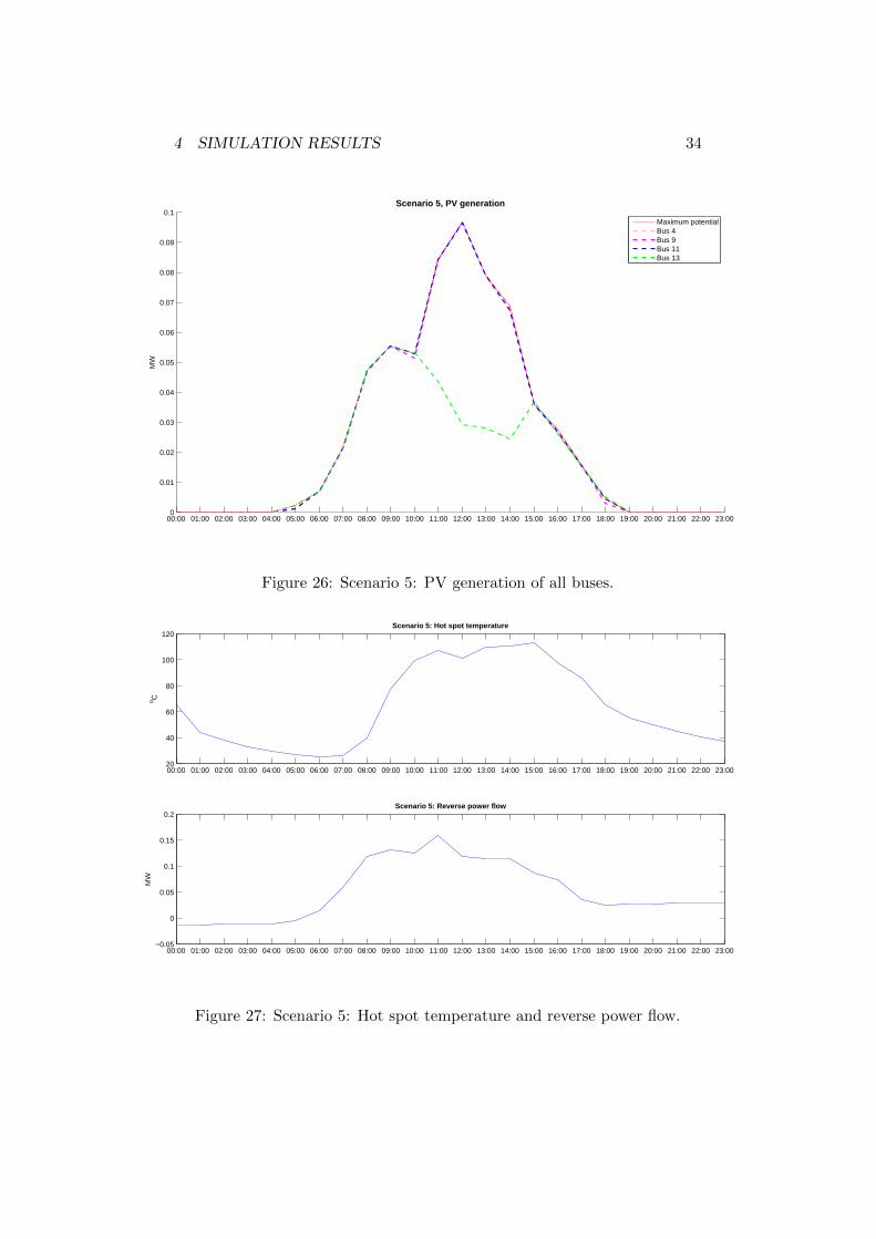
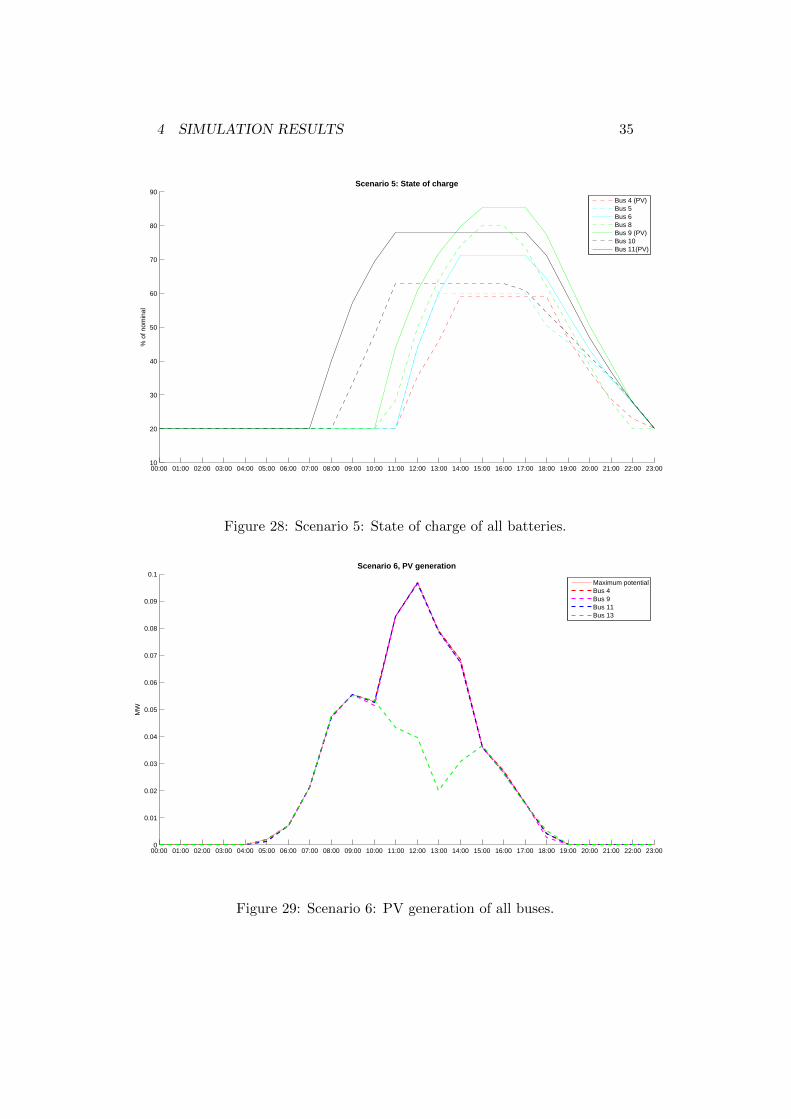
By upgrading the conductor in scenario 5, the PV yield increases becausethe PV generation is limited only for bus 13 between 11:00- 14:00. Duringthese hours overvoltage is observed on the same bus as well as on bus 11for one hour (11:00). In this case, the generation of bus 4 is not constraintso the algorithm does not allocate storage to it but suggests additionally tobuses 5 and 8. Overall, storage is suggested on buses 5 and 8 - 13. The stateof charge level is almost the same in all these buses with the exception ofbus 11 which rises at 24% more. Buses 5 and 8 are allocated with 60%.

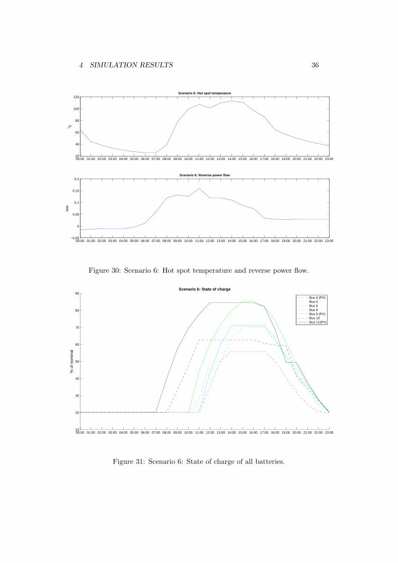
In scenario 6, everything remains the same besides the voltage profile.Overvoltage is observed for one fewer hour on bus 13. For this hour (20:00)the overvoltage moves to bus 12. At 11:00 an overvoltage is also observedat bus 11.

4.3 Transformer

θh follows a similar trend in all scenarios. The initial loading of the trans-former is 70% which is higher than the loading it can get during the firsthours of the day when no PV generation exists and the ambient temperatureis low. Therefore until 06:00 theta hot drops. It starts rising one hour afterPV generation begins and keeps rising until around 15:00. The hot temper-ature follows the trend of reverse power flow but with a delay which can beattributed to the oil time constant which is 3h and the discrete transformer


00:00 01:00 02:00 03:00 04:00 05:00 06:00 07:00 08:00 09:00 10:00 11:00 12:00 13:00 14:00 15:00 16:00 17:00 18:00 19:00 20:00 21:00 22:00 23:000

0.01

0.02

0.03

0.04

0.05

0.06

0.07

0.08

0.09

0.1

MW




00:00 01:00 02:00 03:00 04:00 05:00 06:00 07:00 08:00 09:00 10:00 11:00 12:00 13:00 14:00 15:00 16:00 17:00 18:00 19:00 20:00 21:00 22:00 23:0020

40

60

80

100

120

o C


00:00 01:00 02:00 03:00 04:00 05:00 06:00 07:00 08:00 09:00 10:00 11:00 12:00 13:00 14:00 15:00 16:00 17:00 18:00 19:00 20:00 21:00 22:00 23:00−0.05

0

0.05

0.1

0.15

0.2

MW




00:00 01:00 02:00 03:00 04:00 05:00 06:00 07:00 08:00 09:00 10:00 11:00 12:00 13:00 14:00 15:00 16:00 17:00 18:00 19:00 20:00 21:00 22:00 23:0010

20

30

40

50

60

70

80

90

% o

f nom

inal


Bus 4 (PV)Bus 5Bus 6Bus 8Bus 9 (PV)Bus 10Bus 11(PV)


00:00 01:00 02:00 03:00 04:00 05:00 06:00 07:00 08:00 09:00 10:00 11:00 12:00 13:00 14:00 15:00 16:00 17:00 18:00 19:00 20:00 21:00 22:00 23:000

0.01

0.02

0.03

0.04

0.05

0.06

0.07

0.08

0.09

0.1

MW





00:00 01:00 02:00 03:00 04:00 05:00 06:00 07:00 08:00 09:00 10:00 11:00 12:00 13:00 14:00 15:00 16:00 17:00 18:00 19:00 20:00 21:00 22:00 23:0020

40

60

80

100

120

o C


00:00 01:00 02:00 03:00 04:00 05:00 06:00 07:00 08:00 09:00 10:00 11:00 12:00 13:00 14:00 15:00 16:00 17:00 18:00 19:00 20:00 21:00 22:00 23:00−0.05

0

0.05

0.1

0.15

0.2

MW



00:00 01:00 02:00 03:00 04:00 05:00 06:00 07:00 08:00 09:00 10:00 11:00 12:00 13:00 14:00 15:00 16:00 17:00 18:00 19:00 20:00 21:00 22:00 23:0010

20

30

40

50

60

70

80

90

% o

f nom

inal


Bus 4 (PV)Bus 5Bus 6Bus 8Bus 9 (PV)Bus 10Bus 11(PV)


5 CONCLUSIONS 37

Bus 4 (PV) Bus 5 Bus 8 Bus 9 (PV) Bus 10 Bus 11(PV) Bus 12 Bus 13(PV)0

10

20

30

40

50

60

70

80

90Maximum state of charge

% o

f nom

inal

Scenario 4Scenario 5Scenario 6

Figure 32: Optimal sizing of batteries of all scenarios. Optimal size is as-sumed the maximum capacity of battery reached during the whole optimiza-tion time horizon.

model used which takes under consideration for each time step, the previousone. The transformer’s thermal limits are reached only in scenario 6.

5 Conclusions

Due to environmental concerns, more and more renewable energy resourcesare installed. As the regulatory incentives are encouraging distributed gen-eration, the question of what is the impact of the increasing penetration tothe grid rises. Photovoltaic generation is highly suitable for such applica-tions, therefore in this project we are focusing on this form of distributedgeneration.

In the present project, the potential impacts of high penetration and rel-evant mitigation strategies are reviewed while in steady-state and assumingthree-phase symmetrical operation. Their advantages and disadvantages arepresented. Out of all possibilities, mitigation through storage and conductorupgrading are further investigated.

At the second part, a low voltage grid with high penetration of PVgeneration is investigated. Six simulation scenarios are run with differentconductors and storage possibility or not. The optimization algorithm isconstrained by the overvoltages, the thermal limits of the cables and the

5 CONCLUSIONS 38

00:00 01:00 02:00 03:00 04:00 05:00 06:00 07:00 08:00 09:00 10:00 11:00 12:00 13:00 14:00 15:00 16:00 17:00 18:00 19:00 20:00 21:00 22:00 23:0020

40

60

80

100

120

140

o C

Transformer: Hot spot temperature

Scenario 1Scenario 2Scenario 3Scenario 4Scenario 5Scenario 6

Figure 33: Hot spot temperature of all scenarios.

thermal limit of the transformer.It is clear, based on the simulations scenarios, that by upgrading the

conductor, more PV yield can be extracted in total. However, adding storageis more preferable than upgrading the conductor when it comes to solar yield.By upgrading the conductor, one can see that both for the non-storage andthe storage scenarios, more PV generation is achieved reaching 91.3% outof the maximum potential as opposed to 68.3% at the first (base) scenario.

It is also of interest to observe the allocation of PV yield across the grid.In all scenarios it is observed that the most PV generation is allocated closerto the feeder rather that at lower part of the grid where the generation isconstrained by the overvoltages. Upgrading the conductor leads to fewerovervoltages in terms of duration and/or buses. The more close to thefeeder, the more likely it is for the PV generation to be constrained duringthe peak solar radiation hours by the thermal limits of the cables and/orthe transformer.

In all three storage scenarios, the algorithm suggests higher allocationof capacity to the bottom of the grid. As expected, storage is in no casesuggested for the service cable buses 6 and 7 which are connected to theonly load without PV generator. The allocation of capacity across the gridis clearly related to the fact that it is the further PV generators whose gen-eration is constrained the most. However, it is worthwhile noticing that thealgorithm suggests central allocation of the batteries at the bottom part of

5 CONCLUSIONS 39

the grid, at the early hours, before making full use of the available capacityand before (or without) placing batteries at the top of the grid. This behav-ior is related to the consideration of the voltage profile during the dischargingperiod, the limited optimization horizon and potentially the considerationof the grid losses.

Figure 34: PV penetration in all scenarios.

Figure 35: PV penetration, reverse power flow and battery yield in all sce-narios.

Overall, it is clear that the use of batteries is more advantageous in termsof solar energy yield. Despite the promising results, the cost of the batteriesposes a very important constraint. Given that this project was not meantto present an economical study, it would be interesting in terms of possiblefuture work, for one to extend it by adding financial aspects such as capitaland maintenance cost, regulatory incentives etc

REFERENCES 40

References

[1] R. Tonkoski, L.A.C. Lopes, T.H.M. El-Fouly, Coordinated active powercurtailment of grid connected PV inverters for overvoltage prevention,IEEE Transactions on sustainable energy, vol.2, no.2, April 2011.

[2] S. Conti, S. Raiti, G. Tina, U.Vagliasindi, Integration of multiple PVunits in urban power distribution systems, Elsevier, Science Direct, Solarenergy 75, 2003

[3] C.L. Masters, Voltage rise: the big issue when connecting embeddedgeneration to long 11kV overhead lines, IEE Power Engineering Journal,February 2002

[4] P.M.S. Carvalho, P.F. Correia, L.A.F.M. Ferreira, Distributed reactivepower generation control for voltage rise mitigation in distribution net-works, IEEE Transactions on power systems, vol.23, no.2, May 2008

[5] S.Conti, S.Raiti, Probabilistic load flow using Monte Carlo techniquesfor distribution networks with photovoltaic generation, Elsevier, ScienceDirect, Solar energy 81, 2007

[6] R. Tonkoski, L.A.C. Lopes, voltage regulation in radial distribution feed-ers with high penetration of photovoltaic, IEEE Energy2030, November2008

[7] S. Toma, T. Senjyu, Y. Miyazato, A. Yona, T. Funabashi, A. YousufSaber, C. Kim, Optimal coordinated voltage control in distribution sys-tem, IEEE power and energy society general meeting conversion anddelivery of electrical energy in the 21st century, 2008

[8] E. Demirok, R.Teodorescu, U.Borup, D.Sera, P.Rodriguez, Evaluationof the voltage support strategies for the low voltage grid connected pvgenerators, Energy Conversion Congress and exposition (ECCE), IEEE,2010

[9] G.Andersson, Dynamics and control of electric power systems , EEHPower Systems Laboratory, ETH Zurich, February 2012

[10] M.R. Salem, L.A. Talat, H.M.Soliman, Voltage control by tap-changingtransformers for a radial distribution network, Generation, Transmissionand Distribution, IEE Proceedings, Vol.144, Issue 6, 1997

[11] P.Trichakis, P.C.Taylor, P.F. Lyons, R.Hair, Predicting the technicalimpacts of high levels of small-scale embedded generators on low-voltagenetworks, IET Renewable power generation, 2008

REFERENCES 41

[12] IEEE power engineering society, IEEE Standard for calculating thecurrent-temperature of bare overhead conductors, IEEE Std 738-2006

[13] M. Heathcote, J & P Transformer Book , Newnes by Elsevier, 13thedition, 2007

[14] L.M. Cipcigan, P.C.Taylor, Investigation of reverse power flow require-ments of high penetrations of small-scale embedded generation, IET Re-newable power generation, 2007

[15] V.Levi, M. Kay, I. Povey, Reverse power flow capability of tap-changers,CIRED, 18th International conference on electricity distribution, Turin,June 2005

[16] M. McGranagham, T. Ortmeyer, D.Crudele, Th. Key, J.Smith, Ph.Barker,Renewable systems interconnection study: Advanced grid plan-ning and operation, Sandia Report, February 2008

[17] Distributed generation impact: Sympathetic tripping of protective de-vices, http://pterra.us/blog2/archives/272

[18] E.Larsen, Backfeeding ground fault circuit breakers, Schneider electric,February 2012

[19] Technical publication, Reverse-feed applications for circuit breakers,EATON Power business worldwide, May 2010

[20] H. Chen, T. N. Cong, W. Yang, C. Tan, Y. Li, Y. Ding, Progress inelectrical energy storage system: a critical review, Elsevier 2009

[21] S. Papathanasiou, N. Hatziargyriou, K.Strunz, A benchmark low volt-age microgrid network, CIGRE Symposium Power systems with dis-persed generation: technologies, impacts on development, operation andperformances, April 2005

[22] PV LIB Toolbox http://pvpmc.org/pv-lib/

[23] E.I.Vrettos, S.A.Papathanassiou, Operating policy and optimal sizingof a high penetration RES-BESS system for small isolated grids, IEEETransaction on energy conversion, vol. 26, no.3, September 2011

[24] International standard, Power transformers- Part 7: Loading guide foroil-immersed power transformers, CEI IEC 60076-7, 1st edition 2005

[25] M.Kuss, T.Markel, W. Kramer, Application of distribution transformerthermal life models to electrified vehicle charging loads using Monte-Carlo method, NREL, January 2011

[26] IEA report, Overcoming PV grid issues in urban areas, October 2009

http://pterra.us/blog2/archives/272

http://pvpmc.org/pv-lib/

REFERENCES 42

[27] YALMIP Wiki,What is YALMIP: http://users.isy.liu.se/

johanl/yalmip/pmwiki.php?n=Main.WhatIsYALMIP

[28] YALMIP Wiki, IPOPT: http://users.isy.liu.se/johanl/yalmip/pmwiki.php?n=Solvers.IPOPT

http://users.isy.liu.se/johanl/yalmip/pmwiki.php?n=Main.WhatIsYALMIP

http://users.isy.liu.se/johanl/yalmip/pmwiki.php?n=Main.WhatIsYALMIP

http://users.isy.liu.se/johanl/yalmip/pmwiki.php?n=Solvers.IPOPT

http://users.isy.liu.se/johanl/yalmip/pmwiki.php?n=Solvers.IPOPT

impacts of high penetration of pv in distribution grids ... · 2.1.5 storage by storing energy...

Documents