impacts of cash crop production on land management and land degradation
TRANSCRIPT
Impacts of Cash Crop Production on Land Management and Land Degradation: The Case
of Coffee and Cotton in Uganda
John Pender1, Ephraim Nkonya1, Edward Kato1, Crammer Kaizzi2 and Henry Ssali2
John Pender, International Food Policy Research Institute
Corresponding author: John Pender, [email protected] 1 International Food Policy Research Institute, 2033 K Street NW, Washington D.C. 20006
2 Kawanda Agricultural Research Institute, P.O. Box 7065 Kampala, Uganda 3 Independent consultant, P.O. Box 23097 Kampala, Uganda
Contributed Paper prepared for presentation at the International Association of Agricultural
Economists Conference, Beijing, China, August 16-22, 2009
Copyright 2009 by John Pender, Ephraim Nkonya, Edward Kato, Crammer Kaizzi and Henry Ssali. All rights reserved. Readers may make verbatim copies of this document for non-commercial purposes by any means, provided that this copyright notice appears on all such copies.
1
Abstract We investigate the impacts of coffee and cotton production on land management and land degradation in Uganda, based on a survey of 851 households and soil measurements in six major agro-ecological zones, using matching and multivariate regression methods. The impacts of cash crop production vary by agro-ecological zones and cropping system. In coffee producing zones, use of organic inputs is most common on plots growing coffee with other crops (mainly bananas), and least common on mono-cropped coffee. Both mono-cropped coffee and mixed coffee plots have lower soil erosion than other plots in coffee producing zones because of greater soil cover. Potassium depletion is much greater on mixed banana-coffee plots. In the cotton production zone, few land management practices or investments are used, especially on cotton plots. Soil erosion and soil nutrient depletion are lower in the cotton zone than in coffee producing zones because of flatter terrain and lower crop yields. Soil erosion is much higher on cotton than non-cotton plots in this zone. These results imply that promotion of cash crop production will not halt land degradation, and in some cases will worsen it, unless substantial efforts are made to promote adoption of sustainable land management practices. Key words: land management, land degradation, soil nutrient depletion, soil erosion, agricultural commercialization, cash crops, Uganda JEL: Q13, Q16, Q17
2
Introduction
Land degradation is a severe problem in Uganda, as elsewhere in sub-Saharan Africa. The rate
of soil nutrient depletion in Uganda in among the highest in Africa (Henao and Baanante 2006)
because of very limited use of organic or inorganic sources of fertility. The rate of fertilizer use
in Uganda is among the lowest in the world, averaging only 1 kg of soil nutrients per hectare in
the 1990s (NARO and FAO 1999). Soil erosion is severe in many sloping areas. For example,
Rücker (2005) estimated that net soil loss since the 1960s averaged 21 tons/ha/year in a
cultivated site in the eastern highlands, with rates as high as 45 tons/ha/year on the more steeply
sloping portions of the site, while similar erosion rates have been measured in erosion plots on
sloping lands in central Uganda (Zake and Nkwiine 1995).
Land degradation is contributing to low and declining productivity in Uganda, and hence
is undermining efforts to reduce poverty. According to one recent study, Ugandan farmers
deplete on average about 1.2 percent of the soil nutrient stock in their topsoil each year, causing
a productivity decline of 0.3 percent (Nkonya, et al. 2005). Ugandan farmers depend on soil
nutrient mining for about one-fifth of their farm income on average (Ibid.).1
The main response to low agricultural productivity and rural poverty by policy makers in
Uganda (and many other African countries) is to promote agricultural modernization and
commercialization. Promotion of high value cash crop production2 is often seen as the solution
to land management problems since farmers are expected to have more incentive and ability to
finance use of fertilizer and organic inputs and to make land improving investments on cash
crops than on subsistence food crops.
There is significant evidence supporting this presumption. For example, Tiffen,
Mortimore and Gichuki (1994) found that farmers in the Machakos district of Kenya adopted
higher value cash crops and more intensive soil and water conservation practices, resulting in
higher incomes and less erosion as population grew and access to market opportunities improved
over a 50 year period. Place, et al. (2006) found a similar pattern of improving land
management and incomes in the highlands of central Kenya associated with shifts to production
of higher value commodities, including coffee, tea and dairy production; in contrast to
1 This is the value of soil nutrient depletion with nutrients valued at their replacement cost, using the cheapest available fertilizers. 2 We define a cash crop as a crop grown primarily for sale, as distinct from food crops, which are consumed at home as well as (in most cases) sold by farm households.
3
continuing land degradation in subsistence food production systems of western Kenya. In
Uganda, Pender, et al. (2004) found that adoption of organic land management practices and
perceived improvements in resource and welfare conditions were greater where coffee and
banana production were expanding than in other development pathways. Nkonya, et al. (2004)
also found favorable impacts of cash crop production on adoption of several land management
practices in Uganda, while Pender, et al. (2001) found similar favorable impacts of perennial
cash crop production in the Ethiopian highlands. In West Africa, Mortimore (2005) found
improving land management in rural areas around the city of Kano in Nigeria, associated with
production of cash crops such as groundnuts, livestock and increasing off-farm employment
opportunities.
Positive impacts of market development and cash crop production on land management
are by no means a universal finding, however. For example, in a review of several studies of
land management in the East African highlands, Pender, Place and Ehui (2006) found many
examples in which better market access or cash crop production was associated with less
adoption of improved land management practices. For example, Benin (2006) found that
farmers in the Amhara region were less likely to use reduced tillage or contour plowing closer to
roads; Pender and Gebremedhin (2007) found less use of contour plowing closer to towns in
Tigray; and Jagger and Pender (2006) found less incorporation of crop residues or use of mulch
closer to towns in Uganda.
Furthermore, better market access and cash crop production can contribute to land
degradation even if these promote greater adoption of improved land management practices,
because better access and greater market orientation can increase the outflows of nutrients from
the farm through crop sales, and because cash crops may be more erosive than food crops. For
example, de Jager, et al. (1998) found that more market oriented farms had much more negative
soil nutrient balances in three districts of Kenya, even though they used more inorganic fertilizer.
They found that nutrient balances varied substantially across types of crops, with maize and
beans plots having higher rates of nutrient depletion than coffee or tea plots (though the
differences weren’t statistically significant given their small sample), while depletion was much
larger on napier grass plots than plots growing other crops. Nkonya, et al. (2004) found that soil
nutrient depletion in maize systems of eastern Uganda was greater in villages closer to markets,
4
mainly because the outflows of harvested products were much greater in these areas and not
compensated by increased nutrient inflows.
Clearly, the question of what impacts production of cash crops and commercialization of
food crops have on land management and land degradation is not a settled issue. In this paper,
we investigate the first part of this question, focusing on the impacts of cash crop production on
land management and land degradation in Uganda. We investigate the impacts of coffee and
cotton production because these are the two most important cash crops grown in Uganda. We
contribute to the literature on this issue is several ways. First, unlike previous studies, our
analysis is based on a large survey (851 households and more than 3,700 plots) conducted in
several important farming systems of Uganda. Secondly, we investigated not only land
management practices or perceptions of changes in resource conditions, as in several studies, but
also estimated soil erosion and nutrient balances at the plot level based on detailed information
collected in the survey and measurements and soil samples collected from each plot, and then
related these outcomes to the choice of crop at the plot level. Although such work has been done
in some studies such as de Jager, et al. (1998) and Nkonya, et al. (2004), those studies were
much smaller in scale and did not identify comparable counterfactual (non-cash crop) plots for
comparison to cash crop plots. In this study, we analyzed these data using several econometric
matching and regression methods to control for selection biases, and investigated the robustness
of our findings to alternative methods.
The remainder of the paper is organized as follows. Section 2 presents information on
the agro-ecological zones and farming systems in Uganda, section 3 discusses the methods of
data collection and analysis used, section 4 presents the results, and section 5 concludes.
1. Agro-ecological zones and farming systems in Uganda
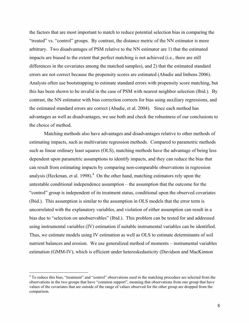
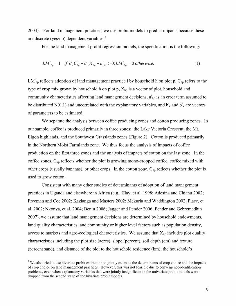
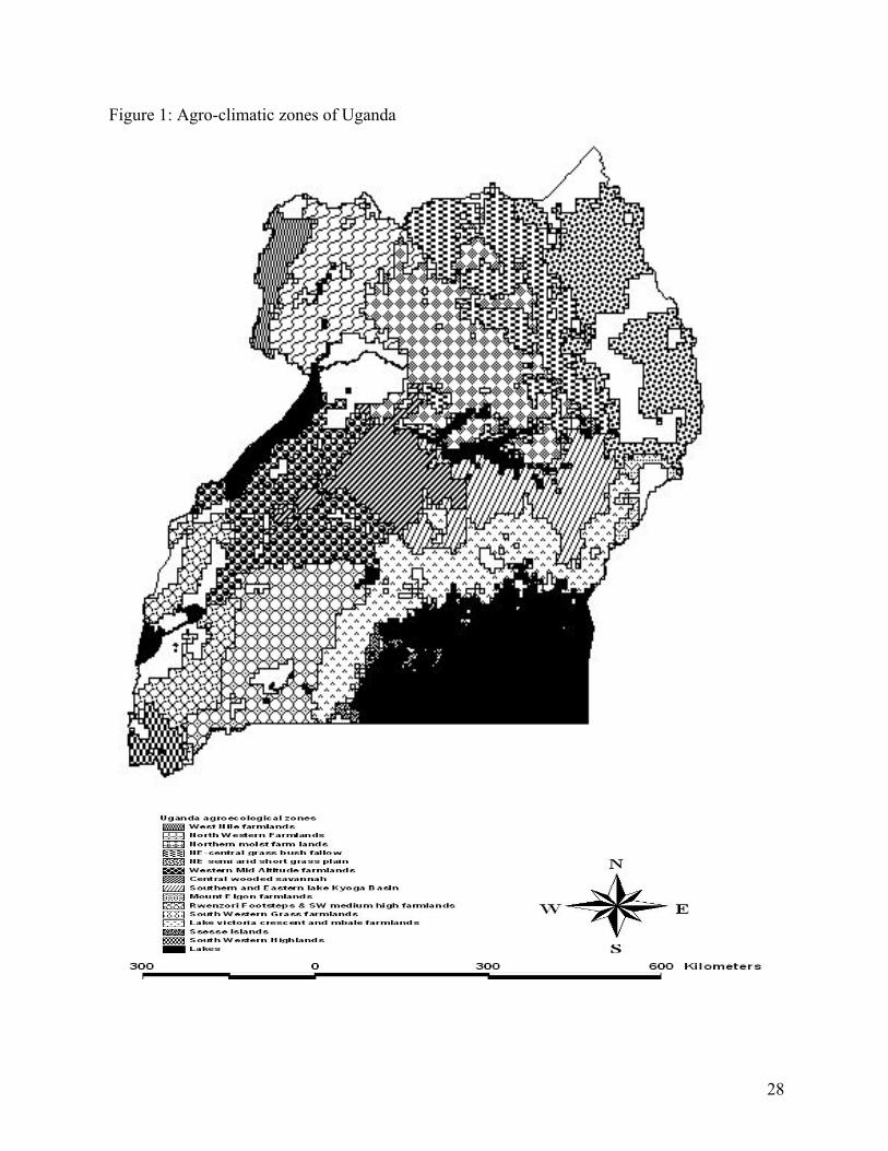
Wortmann and Eledu (1999) classified 14 major agro-ecological zones in Uganda (Figure 1).
These categories are largely determined by the amount of rainfall, which drives agricultural
potential and farming systems in each category. Our surveys were conducted in eight districts
representing six of the most populated zones:
(i) The Lake Victoria Crescent zone has a high level of rainfall (above 1200 mm/year)
distributed throughout the year in a bimodal pattern. Agricultural production is
dominated by the banana-coffee farming system. The zone runs along the vicinity of
5
Lake Victoria from the east in Mbale district, through the central region to Rakai
district in southwestern Uganda along the shores of Lake Victoria.
(ii) Northwest farmland zone: This area is characterized by unimodal low to medium
rainfall and covers the west Nile districts of Arua, Nebbi and Yumbe. Common crops
grown in the zone are coarse grain (sorghum, millet, bulrush, etc), maize, tubers, and
tobacco. The region covers areas with high rainfall in the highlands (above 1200
mm/year) and medium rainfall in the lowlands plans (900 – 1200mm/year).
(iii) North-moist farmland: This zone is also characterized by unimodal low to medium
rainfall (700 – 1200 mm/year) and covers most of the northern districts. The area has
sandy soils with low inherent fertility. The common crops grown are coarse grain,
maize, tubers, cotton, and a variety of legumes.
(iv) Mount Elgon farmlands: This zone is on the slopes of Mount Elgon in the east and is
characterized by unimodal high (above 1200 mm/year) and well distributed rainfall,
high altitude and hence cooler temperatures, and relatively fertile volcanic soils. The
main districts in this zone are Mbale and Kapchorwa. The major crops in this zone
include maize, bananas and coffee.
(v) Southwestern grass-farmland: This zone receives medium to low rainfall (900 – 1200
mm/year) in a bimodal distribution. The region is along the cattle corridor area with
mainly Savannah vegetation suitable to livestock grazing. Farmers in this zone keep
large herds of cattle and grow bananas, coffee, coarse grains, maize and tubers.
(vi) Southwestern highlands (SWH) zone. This zone receives bimodal high rainfall (above
1200 mm/year) and has high altitude, hence cooler climate, and relatively fertile
volcanic soils. Some areas in the lowlands receive medium rainfall ranging from 900
– 1200 mm/year. The common crops in the southwestern highlands are bananas, Irish
potatoes and other tubers, sorghum, maize, and vegetables.
Our analysis focuses on the zones where coffee and cotton are primarily produced: the
Lake Victoria Crescent, Mt. Elgon Farmlands, and Southwest Grasslands for coffee, and the
Northern Moist Farmlands for cotton.
6
3. Methods
In this section we discuss the sources of data and methods of analysis used.
3.1. Data
The data used in this study included data collected from the Uganda Bureau of Statistics (UBOS)
and data from a community, household and plot level survey. The surveys were conducted with
a sub-sample of the enumeration areas and households included in the UBOS 2002/03 Uganda
National Household Survey (UNHS). A stratified two-stage sample was drawn for the UNHS.
Using the 56 districts as strata, 972 enumeration areas (565 rural and 407 urban) were randomly
selected at the first stage sampling, from which a total of 9,711 households were randomly
selected in the second stage sampling. Some of the data used in the econometric analysis in this
study are from the UNHS and the Uganda 2002 Population Census.
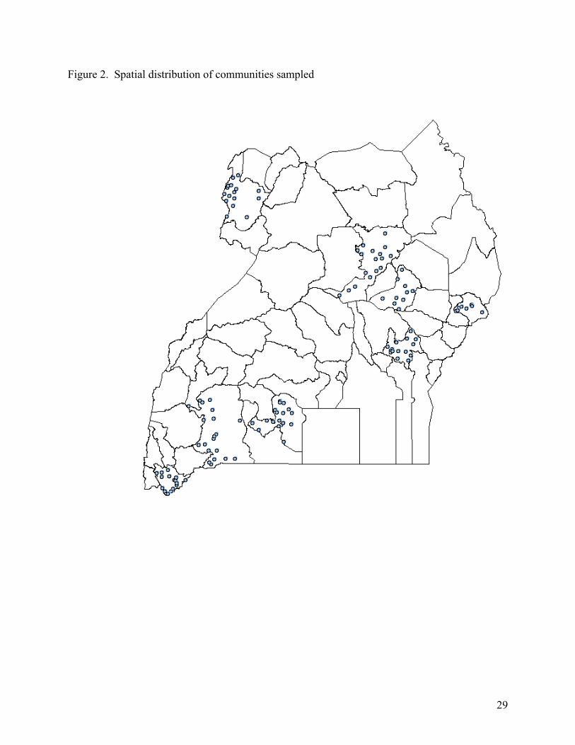
Most of the data used in this study are derived from a smaller survey conducted by IFPRI
and UBOS in 123 communities in 2003, which were drawn from the 565 rural enumeration areas
that were covered by the UNHS. This smaller survey drew a sample using the rural enumeration
areas in eight districts as the sampling frame. The districts selected for the IFPRI-UBOS survey
were: Arua, Iganga, Kabale, Kapchorwa, Lira, Masaka, Mbarara, and Soroti. These districts
were selected to represent different levels of poverty and natural resource endowments, and
major agro-ecologies and farming systems in Uganda. Figure 1 shows the spatial distribution of
the sampled communities.
In each selected enumeration area, we randomly selected seven of the UNHS sample
households for the IFPRI-UBOS survey. The survey focused on questions that were not already
available from the UNHS, particularly issues related to land management and land degradation.
For each household, information was collected on all plots operated by the household, including
the location of the plot, land use and types of crops, use of land management practices and land
investments, inputs into and outputs from the plot, and others.
For crop plots, detailed measurements were taken in the field, including measurements of
the plot size (using Global Positioning Units), slope (using clinometers), and topsoil depth. Soil
samples were collected from the top 20 cm of the soil and analyzed by soil scientists at the soils
laboratory of the Uganda National Agricultural Research Organization (NARO). These data,
together with the survey data, were used to estimate soil nutrient stocks, inflows and outflows of
soil nutrients from each plot, using the methods described by Smaling, et al. (1993) and de Jager,
7
Nandwa and Okoth (1998).3 In estimating soil nutrient outflows, soil erosion rates were
estimated using the Revised Universal Soil Loss Equation (RUSLE) (Renard, et al. 1991), which
has been calibrated and validated in several studies in Uganda (Lufafa, et al., 2003; Mulebeke,
2003; Majaliwa, 2003; Tukahirwa, 1996).
3.2. Analysis
We analyzed the differences in land management practices, soil erosion and soil nutrient
depletion across plots growing coffee, cotton and other crops using simple descriptive statistics
and econometric methods to account for differences in the characteristics of the plots and in
agro-ecological and socioeconomic environments that may affect these outcomes. The
econometric methods that we used included matching estimators and multivariate regression
methods.
Matching methods are designed to identify the impacts of a discrete factor on outcomes
of interest by selecting comparable “treatment” and “control” observations in terms of
observable characteristics expected to jointly influence the selection of observations into these
categories and the outcomes. Although often used to evaluate impacts of programs (e.g.,
Heckman, et al. 1997; Ravallion 2005), such methods can also be used to assess impacts of other
discrete factors, such as impacts of land management practices (Kassie, et al. 2008). In our case,
we used matching estimators to assess the impacts of plot level crop choice on land management
and land degradation indicators.
The matching estimators used in our analysis include propensity score matching (PSM)
(Rosenbaum and Rubin 1983) and the bias-corrected nearest neighbor matching (NN) estimator
developed by Abadie, et al. (2004). Both methods use a distance metric based on observed
covariates to select comparable “treatment” vs. “control” observations for comparison. PSM
uses the predicted probability of an observation being in the “treated” vs. “control” category as
the distance metric. NN uses a distance metric based on the magnitudes of differences in the
values of the covariates, weighted by the inverse of the variance matrix, which accounts for
differences in scale of the covariates.
Each of these methods has advantages and disadvantages. An advantage of PSM is that
its distance metric gives greater weight to factors that influence the selection process, which are
3 The methods used to estimate soil nutrient flows and balances are described in detail in Kaizzi, Ssali and Kato (2004).
8
the factors that are most important to match to reduce potential selection bias in comparing the
“treated” vs. “control” groups. By contrast, the distance metric of the NN estimator is more
arbitrary. Two disadvantages of PSM relative to the NN estimator are 1) that the estimated
impacts are biased to the extent that perfect matching is not achieved (i.e., there are still
differences in the covariates among the matched samples), and 2) that the estimated standard
errors are not correct because the propensity scores are estimated (Abadie and Imbens 2006).
Analysts often use bootstrapping to estimate standard errors with propensity score matching, but
this has been shown to be invalid in the case of PSM with nearest neighbor selection (Ibid.). By
contrast, the NN estimator with bias correction corrects for bias using auxiliary regressions, and
the estimated standard errors are correct (Abadie, et al. 2004). Since each method has
advantages as well as disadvantages, we use both and check the robustness of our conclusions to
the choice of method.
Matching methods also have advantages and disadvantages relative to other methods of
estimating impacts, such as multivariate regression methods. Compared to parametric methods
such as linear ordinary least squares (OLS), matching methods have the advantage of being less
dependent upon parametric assumptions to identify impacts, and they can reduce the bias that
can result from estimating impacts by comparing non-comparable observations in regression
analysis (Heckman, et al. 1998).4 On the other hand, matching estimators rely upon the
untestable conditional independence assumption – the assumption that the outcome for the
“control” group is independent of its treatment status, conditional upon the observed covariates
(Ibid.). This assumption is similar to the assumption in OLS models that the error term is
uncorrelated with the explanatory variables, and violation of either assumption can result in a
bias due to “selection on unobservables” (Ibid.). This problem can be tested for and addressed
using instrumental variables (IV) estimation if suitable instrumental variables can be identified.
Thus, we estimate models using IV estimation as well as OLS to estimate determinants of soil
nutrient balances and erosion. We use generalized method of moments – instrumental variables
estimation (GMM-IV), which is efficient under heteroskedasticity (Davidson and MacKinnon
4 To reduce this bias, “treatment” and “control” observations used in the matching procedure are selected from the observations in the two groups that have “common support”, meaning that observations from one group that have values of the covariates that are outside of the range of values observed for the other group are dropped from the comparison.
9
2004). For land management practices, we use probit models to predict impacts because these
are discrete (yes/no) dependent variables.5
For the land management probit regression models, the specification is the following:
1 0; 0 .i i i i ihp c hp x hp hp hpLM if b C b X u LM otherwise= + + > = (1)
LMihp reflects adoption of land management practice i by household h on plot p, Chp refers to the
type of crop mix grown by household h on plot p, Xhp is a vector of plot, household and
community characteristics affecting land management decisions, uihp is an error term assumed to
be distributed N(0,1) and uncorrelated with the explanatory variables, and bic and bi
x are vectors
of parameters to be estimated.
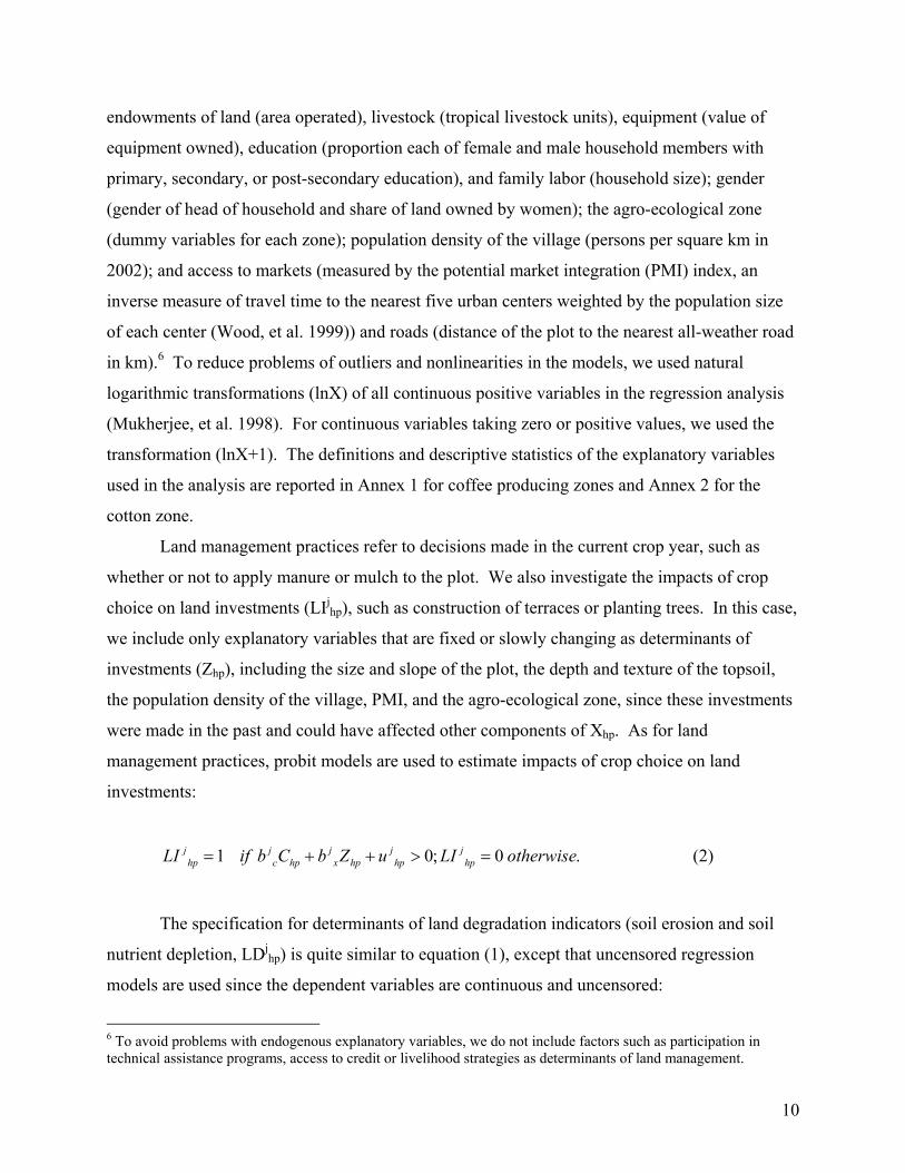
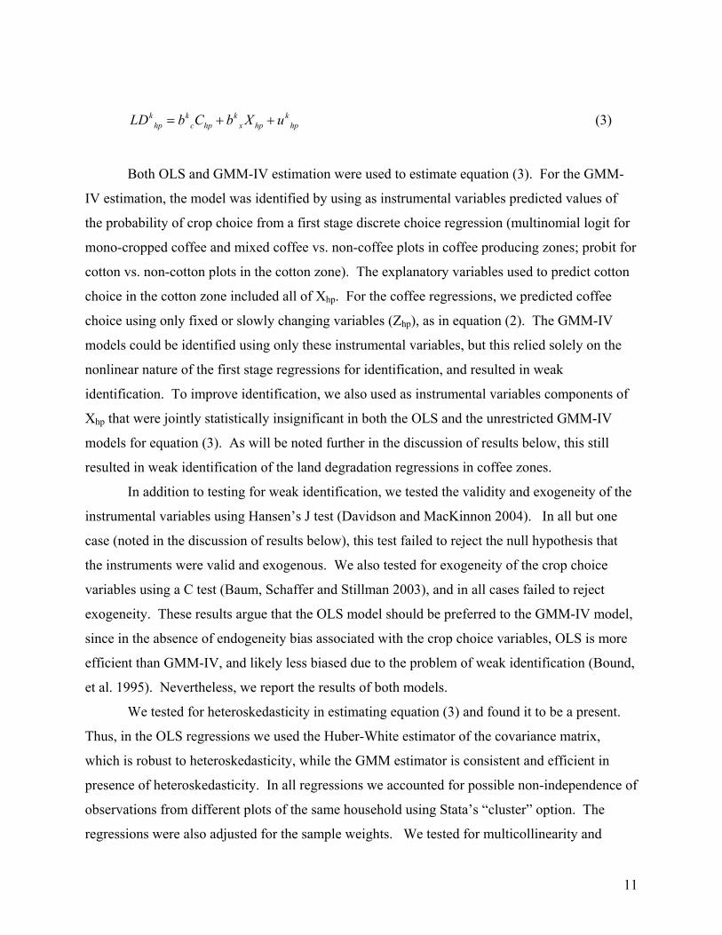
We separate the analysis between coffee producing zones and cotton producing zones. In
our sample, coffee is produced primarily in three zones: the Lake Victoria Crescent, the Mt.
Elgon highlands, and the Southwest Grasslands zones (Figure 2). Cotton is produced primarily
in the Northern Moist Farmlands zone. We thus focus the analysis of impacts of coffee
production on the first three zones and the analysis of impacts of cotton on the last zone. In the
coffee zones, Chp reflects whether the plot is growing mono-cropped coffee, coffee mixed with
other crops (usually bananas), or other crops. In the cotton zone, Chp reflects whether the plot is
used to grow cotton.
Consistent with many other studies of determinants of adoption of land management
practices in Uganda and elsewhere in Africa (e.g., Clay, et al. 1998; Adesina and Chianu 2002;
Freeman and Coe 2002; Kazianga and Masters 2002; Mekuria and Waddington 2002; Place, et
al. 2002; Nkonya, et al. 2004; Benin 2006; Jagger and Pender 2006; Pender and Gebremedhin
2007), we assume that land management decisions are determined by household endowments,
land quality characteristics, and community or higher level factors such as population density,
access to markets and agro-ecological characteristics. We assume that Xhp includes plot quality
characteristics including the plot size (acres), slope (percent), soil depth (cm) and texture
(percent sand), and distance of the plot to the household residence (km); the household’s
5 We also tried to use bivariate probit estimation to jointly estimate the determinants of crop choice and the impacts of crop choice on land management practices. However, this was not feasible due to convergence/identification problems, even when explanatory variables that were jointly insignificant in the univariate probit models were dropped from the second stage of the bivariate probit models.
10
endowments of land (area operated), livestock (tropical livestock units), equipment (value of
equipment owned), education (proportion each of female and male household members with
primary, secondary, or post-secondary education), and family labor (household size); gender
(gender of head of household and share of land owned by women); the agro-ecological zone
(dummy variables for each zone); population density of the village (persons per square km in
2002); and access to markets (measured by the potential market integration (PMI) index, an
inverse measure of travel time to the nearest five urban centers weighted by the population size
of each center (Wood, et al. 1999)) and roads (distance of the plot to the nearest all-weather road
in km).6 To reduce problems of outliers and nonlinearities in the models, we used natural
logarithmic transformations (lnX) of all continuous positive variables in the regression analysis
(Mukherjee, et al. 1998). For continuous variables taking zero or positive values, we used the
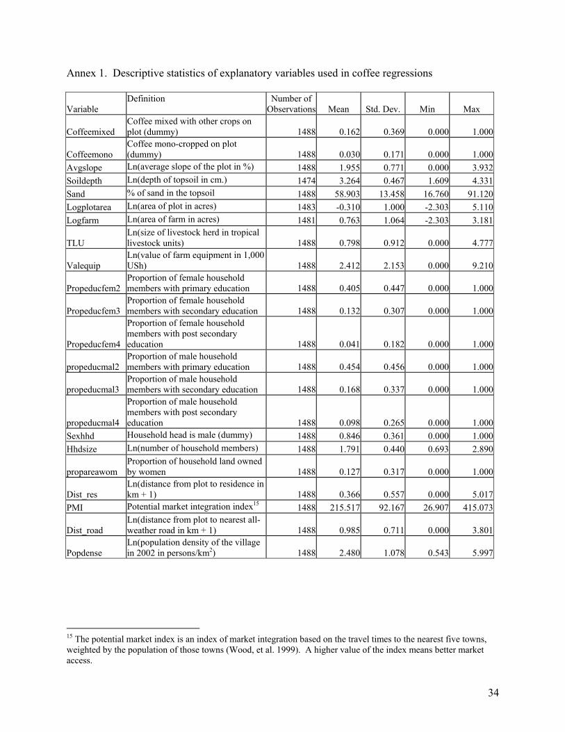
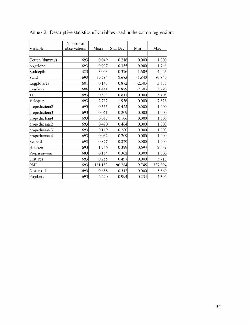
transformation (lnX+1). The definitions and descriptive statistics of the explanatory variables
used in the analysis are reported in Annex 1 for coffee producing zones and Annex 2 for the
cotton zone.
Land management practices refer to decisions made in the current crop year, such as
whether or not to apply manure or mulch to the plot. We also investigate the impacts of crop
choice on land investments (LIjhp), such as construction of terraces or planting trees. In this case,
we include only explanatory variables that are fixed or slowly changing as determinants of
investments (Zhp), including the size and slope of the plot, the depth and texture of the topsoil,
the population density of the village, PMI, and the agro-ecological zone, since these investments
were made in the past and could have affected other components of Xhp. As for land
management practices, probit models are used to estimate impacts of crop choice on land
investments:
1 0; 0 .j j j j jhp c hp x hp hp hpLI if b C b Z u LI otherwise= + + > = (2)
The specification for determinants of land degradation indicators (soil erosion and soil
nutrient depletion, LDjhp) is quite similar to equation (1), except that uncensored regression
models are used since the dependent variables are continuous and uncensored:
6 To avoid problems with endogenous explanatory variables, we do not include factors such as participation in technical assistance programs, access to credit or livelihood strategies as determinants of land management.
11
k k k k
hp c hp x hp hpLD b C b X u= + + (3)
Both OLS and GMM-IV estimation were used to estimate equation (3). For the GMM-
IV estimation, the model was identified by using as instrumental variables predicted values of
the probability of crop choice from a first stage discrete choice regression (multinomial logit for
mono-cropped coffee and mixed coffee vs. non-coffee plots in coffee producing zones; probit for
cotton vs. non-cotton plots in the cotton zone). The explanatory variables used to predict cotton
choice in the cotton zone included all of Xhp. For the coffee regressions, we predicted coffee
choice using only fixed or slowly changing variables (Zhp), as in equation (2). The GMM-IV
models could be identified using only these instrumental variables, but this relied solely on the
nonlinear nature of the first stage regressions for identification, and resulted in weak
identification. To improve identification, we also used as instrumental variables components of
Xhp that were jointly statistically insignificant in both the OLS and the unrestricted GMM-IV
models for equation (3). As will be noted further in the discussion of results below, this still
resulted in weak identification of the land degradation regressions in coffee zones.
In addition to testing for weak identification, we tested the validity and exogeneity of the
instrumental variables using Hansen’s J test (Davidson and MacKinnon 2004). In all but one
case (noted in the discussion of results below), this test failed to reject the null hypothesis that
the instruments were valid and exogenous. We also tested for exogeneity of the crop choice
variables using a C test (Baum, Schaffer and Stillman 2003), and in all cases failed to reject
exogeneity. These results argue that the OLS model should be preferred to the GMM-IV model,
since in the absence of endogeneity bias associated with the crop choice variables, OLS is more
efficient than GMM-IV, and likely less biased due to the problem of weak identification (Bound,
et al. 1995). Nevertheless, we report the results of both models.
We tested for heteroskedasticity in estimating equation (3) and found it to be a present.
Thus, in the OLS regressions we used the Huber-White estimator of the covariance matrix,
which is robust to heteroskedasticity, while the GMM estimator is consistent and efficient in
presence of heteroskedasticity. In all regressions we accounted for possible non-independence of
observations from different plots of the same household using Stata’s “cluster” option. The
regressions were also adjusted for the sample weights. We tested for multicollinearity and
12
found it not to be a serious concern (the maximum variance inflation factor was 8.72 in the
coffee regressions and 2.95 in the cotton regressions).7
For the PSM estimations, we used kernel matching with the epanechnikov kernel
function (the default for Stata’s PSMATCH2 command). For the NN estimations, we used the
default weighting matrix for the distance metric (inverse variance of the covariates) and the five
nearest neighbors in matching. In the matching estimations for coffee producing zones, we used
pairwise matching, comparing mono-cropped plots to non-coffee plots in one estimation, then
comparing mixed coffee plots to non-coffee plots in another estimation for each outcome
variable. For cotton, a single pairwise estimation comparing cotton vs. non-cotton plots was
used for each outcome. The covariates used in the matching estimators were the same as those
used to predict crop choice in the GMM-IV regressions; i.e., we used Xhp as the vector of
covariates for the cotton matching estimators, and the more restricted set of covariates Zhp for the
coffee matching estimators. After the PSM, we conducted balancing tests of how well the
matching reduced differences in the covariates between the “treatment” and “control” groups.
The results of these balancing tests are reported in Annexes 3 and 4. In all cases, the mean
differences in covariates between the matched groups are statistically insignificant and
quantitatively small, despite large differences in covariates in the unmatched groups in some
cases. This indicates that PSM performs well to eliminate systematic differences between the
different groups with respect to the covariates.
4. Results
We first present descriptive statistics on the land management practices and land degradation
indicators in coffee and cotton producing zones, respectively, followed by our econometric
results.
4.1. Land management practices in coffee zones
As noted earlier, the coffee producing zones in our sample include the Lake Victoria crescent,
the Mount Elgon zone, and the Southwest grasslands zone. Of the 294 coffee plots in our survey
sample, 286 were in these three zones. Hence, we limit our analysis of coffee production to 7 For most variables, the variance inflation factor (VIF) was much less than 5 in the coffee regressions; only the agro-ecological zone variables had VIF > 5 in these regressions. The coffee crop choice variables (for mono-cropped coffee and mixed coffee) had had VIF < 1.1, while in the cotton regressions, the cotton choice variable had VIF=1.1. These results indicate that multicollinearity had very little impact on the estimated standard errors of the coefficients for the crop choice variables.
13
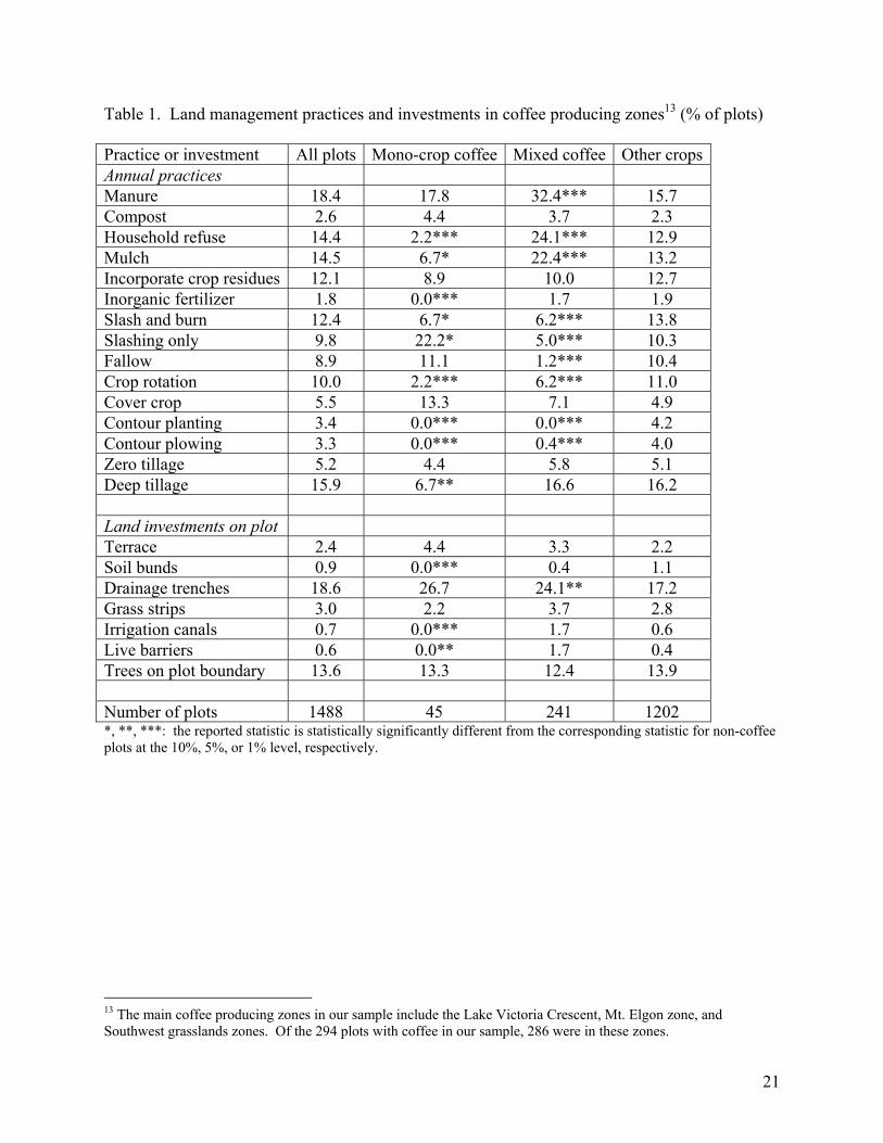
these zones. In these zones, about one fifth of farmers’ plots are growing coffee (Table 1).
Most of these plots are mixed crop plots, including other crops as well as coffee, usually bananas
(80 percent of coffee plots include bananas).
The most common land management practices used in coffee producing zones include
use of organic materials to manage soil fertility, soil moisture and/or weeds (manure, compost,
household refuse, mulch, crop residues); slash and burn or slashing only to clear the plot for
cultivation; fallowing, crop rotation or cover crops to improve soil fertility; alternative tillage
practices such as zero tillage and deep tillage; planting and plowing along slope contours to
conserve soil and water; and inorganic fertilizer. None of these practices is very common; the
most common is application of manure, which is used on less than one fifth of plots. Inorganic
fertilizer is used on less than 2% of plots in these zones.8
There are substantial differences in the land management practices used on mono-
cropped coffee, mixed coffee and other crop plots. In general, application of organic materials is
much more common on mixed coffee plots than on either mono-cropped coffee or other crops.
This is undoubtedly due to the importance of banana production on mixed coffee plots, for which
use of manure, household refuse and mulch is fairly common. This finding is consistent with
findings of other studies on use of land management practices in mixed coffee-banana
production in Uganda (e.g., Pender, et al. 2004; Nkonya, et al. 2004). On mono-cropped coffee
plots, by contrast, use of household refuse and mulch is much less common than on mixed coffee
plots, and even less common than on other crop plots.
Not surprisingly, slash and burn and crop rotation are less common on perennial mono-
cropped coffee and mixed coffee plots than on non-coffee plots, while contour planting and
plowing are virtually non-existent on coffee plots. However, we do find some of these practices
(slash and burn and crop rotation) on some coffee plots; these are probably associated with the
annual crops grown on these plots. Even plots that we have classified as mono-cropped coffee
may only have been mono-cropped in the cropping year covered by our survey. Other annual
crops may be planted on those plots among the coffee trees in other years as part of a crop
rotation or fallow system. This also explains how we find fallowing and tillage practices on
8 We exclude discussion of other even less common land management practices and land investments, found on less than 1 percent of plots of any type (i.e., mono-cropped coffee, mixed coffee or other crops). Examples of such rare practices include alley cropping, improved fallows, and green manures.
14
some coffee plots. We do not find inorganic fertilizer used on any of the mono-cropped coffee
plots and on less than 2 percent of mixed coffee and non-coffee plots.
In addition to these types of regular land management practices, farmers invest in various
types of land improvements. The most common land improvements used are drainage trenches
(found on 27 percent of plots) and planting trees on the plot boundary (on 14 percent).9 The
relatively common use of drainage trenches indicates that managing excess water is a concern in
many areas of the high rainfall coffee producing zones. Drainage trenches are more common on
coffee plots than on non-coffee plots, suggesting that excess water is a particular concern for
coffee. Other less common investments include grass strips, terraces, soil bunds, irrigation
canals and live barriers; all of these are found on 3 percent or fewer of plots in coffee producing
zones. We find no soil bunds, irrigation canals or live barriers on mono-cropped coffee plots,
but these are also relatively rare on other plots. Other investments, such as trees on the plot
boundary, grass strips and terraces are similarly common on coffee and non-coffee plots.
4.2. Land management practices in cotton zones
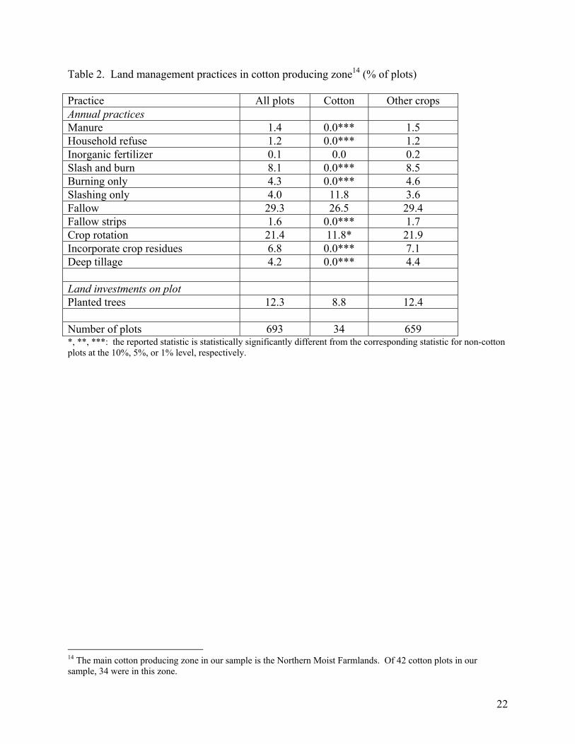
In our sample, cotton is produced primarily in the Northern Moist Farmlands zone, with 34 of the
42 cotton plots in our sample in this zone. About 5 percent of the plots in this zone are cotton
plots (Table 2).
The most common land management practices used in the Northern Moist Farmlands
zone include fallow (29 percent of plots) and crop rotation (21 percent). Other practices used on
at least 1 percent of plots include slash and burn, burning or slashing only, incorporation of crop
residues, deep tillage, fallow strips, and application of manure or household refuse. Inorganic
fertilizer is very rarely used on this zone (0.1 percent of plots). Few of these practices are used
on cotton plots. Only fallow, crop rotation and slashing are used on any cotton plots, and crop
rotation is less common on cotton than on non-cotton plots.
Land investments are also rare in this zone. The only investment that we find on more
than 1 percent of plots is tree planting on the plot. A higher percentage of non-cotton plots have
planted trees than cotton plots, though the difference is not statistically significant.
4.3. Land degradation indicators in coffee and cotton zones
9 In plots growing coffee and other tree crops, farmers of course also plant trees within the plot. We do not include this as a land investment since this is already implied as part of the cropping system.
15
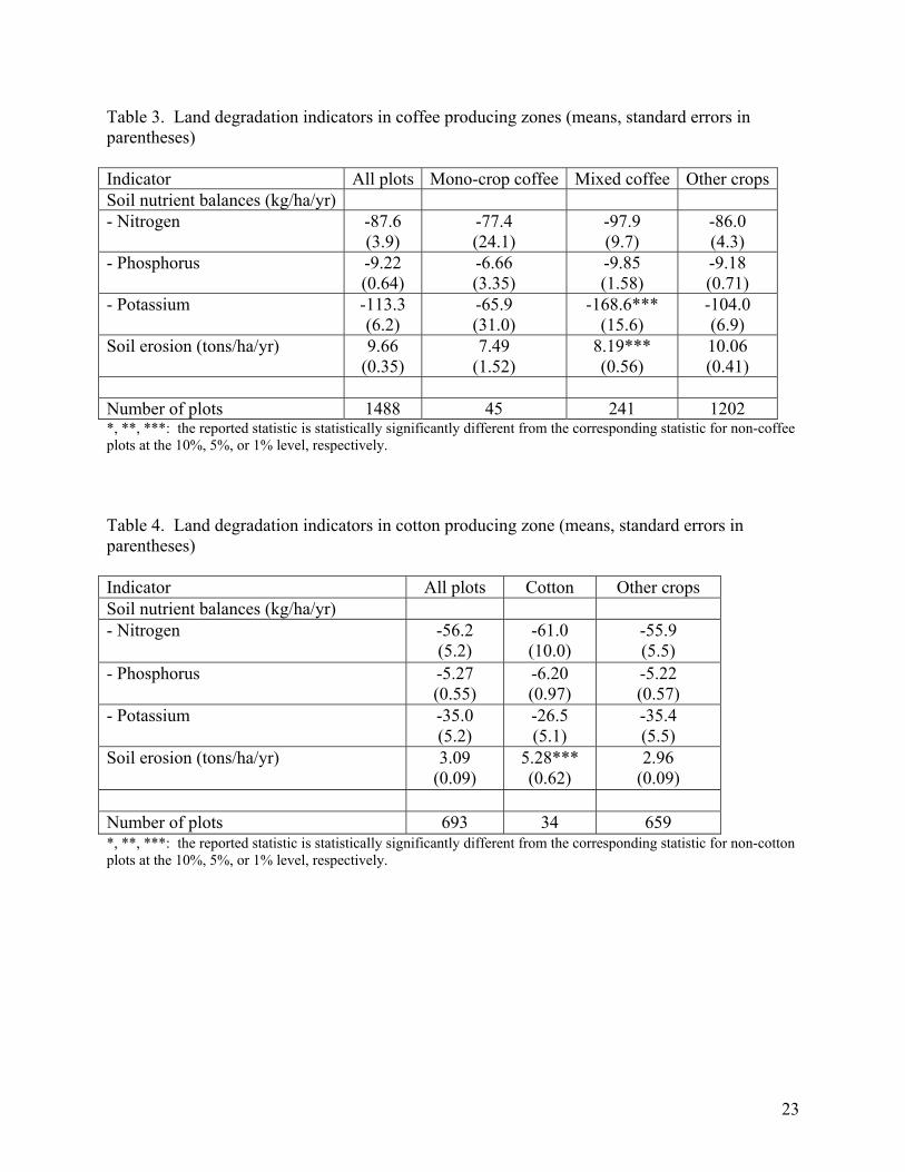
The average estimated soil nutrient balances are negative for N, P and K on all types of plots in
the coffee producing zones, with mean soil nutrient depletion rates of -88 kg/ha/yr for N, -9
kg/ha/yr for P and -113 kg/ha/yr for K (Table 3). These depletion rates are larger than those
estimated for Uganda as a whole by Stoorvogel and Smaling (1990) and Henao and Baanante
(2006), but are more comparable to rates estimated in more micro level studies in East Africa,
which tend to be more negative than the macro scale estimates (Smaling, et al. 1993; Van den
Bosch, et al. 1998; Wortmann and Kaizzi 1998; Nkonya, et al. 2004).
The differences in depletion rates of N and P are statistically insignificant across mono-
cropped coffee, mixed coffee and other crops. However, depletion of K is substantially greater
on mixed coffee plots than on either non-coffee or mono-cropped coffee plots. This is mainly
due to depletion of K through harvests of bananas, which have a high level of K. Thus, even
though organic inputs are most common on mixed coffee plots, as shown in Table 1, and even
though erosion is lower on these plots than non-coffee plots because of their greater soil cover,
potassium depletion is still greater.
Average estimated soil nutrient depletion rates and soil erosion rates are lower in the
Northern Moist Farmland zone than in the coffee producing zones, but still indicate relatively
high rates of soil nutrient depletion – averaging -56, -5 and -35 kg/ha/yr of N, P and K,
respectively (Table 4). Lower erosion is due to the flatter terrain in this zone than in coffee
production zones, despite production of more erosive annual crops. Lower nutrient depletion in
this zone is due to less erosion and lower crop yields, limiting nutrient outflows, despite very
little inflows of organic or inorganic sources of soil nutrients. We find no statistically significant
differences between plots growing cotton vs. other crops in terms of soil nutrient balances.
However, estimated erosion is larger on cotton plots. This is not surprising since soil cover is
low in cotton production due to tillage and intensive weeding of cotton plots.
4.4. Impacts of coffee on land management practices – matching and econometric results
The differences in land management practices between mono-cropped coffee, mixed coffee and
non-coffee plots reported in Table 1 do not control for differences in the nature of the plots, the
households operating them, or the local agro-ecological or socioeconomic environment. Hence
these differences may not reflect the true effects of coffee production on land management. In
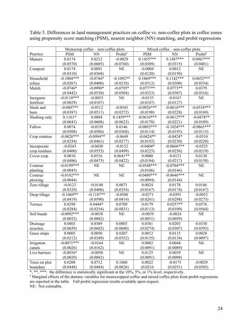
Table 5, we present results of comparisons of land management practices on these different types
of plots using the matching and econometric estimators discussed in section 3.
16
Most of the differences reported in Table 5 are consistent with the simple descriptive
results in Table 1, and are in most cases robust to the estimator used, especially in comparing
mixed coffee and non-coffee plots. The findings of the different estimators are less robust when
comparing mono-cropped coffee and non-coffee plots, probably due to the relatively small
number of mono-cropped coffee plots, which limits the ability to estimate impacts in some cases.
For practices that were used on no mono-cropped coffee plots (e.g., inorganic fertilizer, contour
planting, contour plowing, soil bunds, irrigation canals and live barriers), it was not possible to
estimate the impact of mono-cropped coffee using a probit estimator, and for a few of these the
NN estimator was also not estimable. For several other practices that were used on only a few
mono-cropped coffee plots (e.g., slash and burn, crop rotation), the results were not robust
between the PSM and NN estimator.
Statistically significant results that are robust across all three estimators include the
following: use of household refuse and mulch are less likely on mono-cropped coffee than non-
coffee plots; use of manure and household refuse are more likely on mixed coffee than non-
coffee plots; and use of slash and burn, slashing or burning only, and fallow are less likely on
mixed coffee than non-coffee plots. Results that are robust across the two matching estimators
but not estimable or not significant in the probit model include: crop rotation is less likely on
mono-cropped coffee or mixed coffee plots than on non-coffee plots; deep tillage is less likely on
mono-cropped coffee than non-coffee plots; mulching is more likely on mixed coffee plots than
non-coffee plots; incorporating crop residues, and contour planting and contour plowing are less
likely on mixed coffee plots than non-coffee plots. Some results are estimable and significant
only in the PSM model: inorganic fertilizer, slash and burn, contour planting, contour plowing,
soil bunds and irrigation canals are less likely on mono-cropped coffee than non-coffee plots. A
few results are significant only in the probit models: slashing only and cover crops are more
likely on coffee mono-cropped plots than non-coffee plots.
These results confirm that there are significant differences in land management practices
used on mono-cropped vs. mixed coffee vs. non-coffee plots. Use of organic inputs is most
likely on mixed coffee plots and use of some organic inputs is least likely on mono-cropped
coffee plots. Practices associated with annual crops, such as slash and burn, fallow, crop
rotation, incorporation of crop residues and tillage practices are, not surprisingly, less common
on coffee plots than non-coffee plots.
17
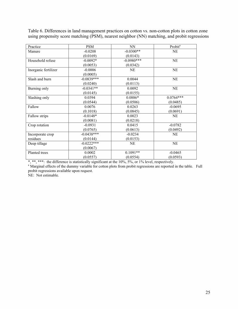
4.5. Impacts of cotton on land management practices – matching and econometric results
The estimated differences between use of land management practices on cotton vs. non-cotton
plots in the Northern Moist Farmlands zone, using the two matching estimators and probit
estimation, are reported in Table 6. For most land management practices, probit estimation
could not estimate this difference because they were not used on any of the cotton plots in our
sample.
Our results are less robust across the three estimators for cotton vs. non-cotton plots than
our results for coffee vs. non-coffee plots. This is likely because of the small number of cotton
plots in our sample. None of the findings were robust across all three estimators, and the only
result that is robust across both matching estimators is that use of household refuse is less likely
on cotton than on non-cotton plots. We find that slashing is more likely on cotton plots using
both the NN matching estimator and the probit estimator. Several other results are significant
only using one estimator: manure use less likely on cotton plots (NN); slash and burn, burning
only, fallow strips, incorporation of crop residues and deep tillage are less likely on cotton plots
(PSM); and tree planting more likely on cotton plots (NN).
Overall, these results support the conclusion that many land management practices are
less common on cotton than non-cotton plots. The one exception is planted trees, for which a
positive association with cotton was found using the NN estimator; but this result was not robust.
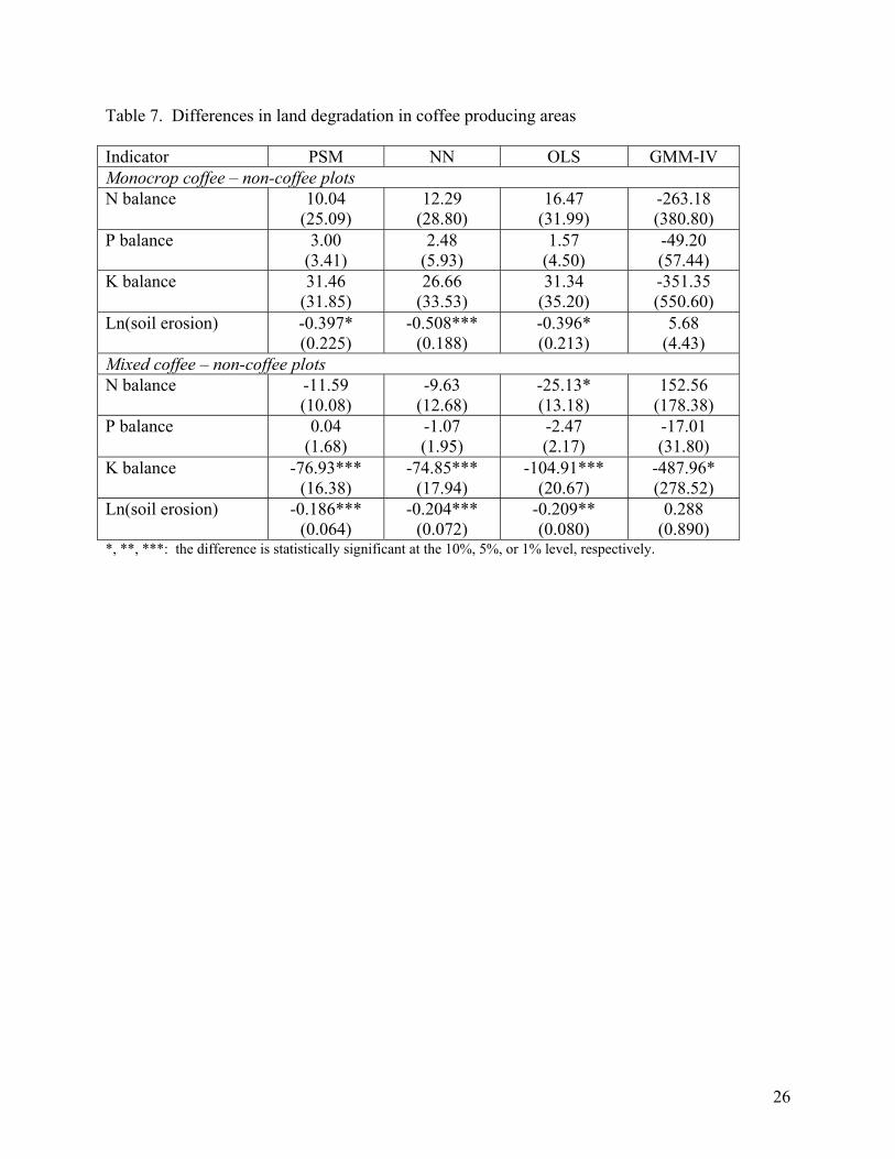
4.6. Impacts of coffee and cotton production on land degradation
The estimated impacts of mono-cropped and mixed coffee production on land degradation
indicators relative to non-coffee plots, using the PSM and NN matching estimators as well as
ordinary least squares (OLS) and generalized method of moments/instrumental variables
regressions (GMM-IV), are shown in Table 7. The results are quite consistent across the two
matching estimators and the OLS model, showing that soil erosion is significantly lower on both
mono-cropped coffee (by 33 – 40 percent, depending on the estimator) and mixed coffee plots
(by 17 – 19 percent) than on non-coffee plots, and that the K balance is more negative on mixed
coffee plots than on non-coffee plots (by -77 to -105 kg of K/ha/year). The negative impact of
mixed coffee on the K balance is also confirmed in the GMM-IV model.
Except for the weakly statistically significant impact of mixed coffee on the K balance in
the GMM-IV model, the estimated impacts of mono-cropped or mixed coffee production on land
degradation indicators in the GMM-IV models are statistically insignificant, despite the
18
coefficients being substantially larger in this model than in the other models in all cases. This is
due to weak identification of these models, leading to much larger standard errors and biased
coefficients (Bound, et al. 1995).10 Since our diagnostic tests with the GMM-IV model support
the validity of the instrumental variables and exogeneity of the explanatory variables, OLS is
preferred over the GMM-IV model as more efficient and subject to less bias.11
These results confirm our observations in Table 3 that potassium depletion is greater on
mixed coffee plots than non-coffee plots, despite lower erosion on these plots, after controlling
for differences between plot characteristics and agro-ecological and socio-economic conditions.
We also find that erosion is lower on mono-cropped coffee than non-coffee plots, consistent with
the estimated mean levels of erosion reported in Table 3 (although the result in Table 3 was not
statistically significant). Hence, we find that coffee production has favorable impacts in
reducing soil erosion due to better soil cover and less tillage than with annual crops. However,
mixed coffee (usually with banana) production has a negative impact on potassium depletion,
despite greater use of organic inputs, primarily due to the effects of banana harvests.
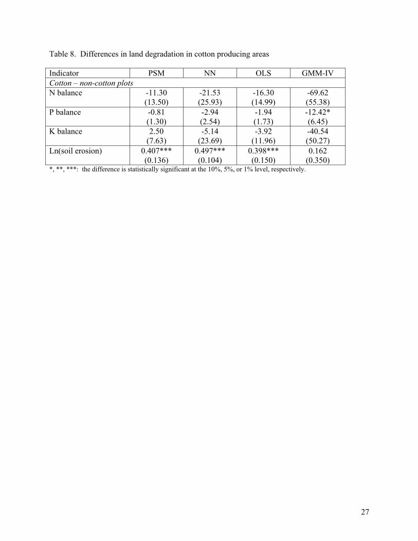
For cotton, we find that erosion is significantly greater on cotton plots than non-cotton
plots (by 49 to 64 percent) using both matching estimators and OLS, while the impact on erosion
in the GMM-IV model is statistically insignificant. We find no statistically significant
differences in soil nutrient depletion on cotton vs. non-cotton plots using the different estimators,
except a weakly significant (10 percent level) impact of cotton production on the P balance using
GMM-IV. As for the coffee regressions, the exogeneity of the explanatory variables was not
rejected in the GMM-IV models for cotton, so OLS is preferred over GMM-IV estimation.12
Except for the GMM-IV results, these results are consistent with the descriptive findings in
Table 4, showing that cotton is more erosive than other crops planted in cotton producing areas.
10 In the first stage of the GMM-IV models, the partial R2 for mono-cropped coffee and mixed coffee variables were only 0.0058 and 0.0048, respectively, and Wald tests of the instrumental variables were statistically insignificant (p = 0.2645 and 0.6161 for mono-cropped coffee and mixed coffee, respectively). Under-identification of these models could not be rejected using the Kleibergen-Paap rk LM statistic (p levels = 0.4062). For an explanation of these diagnostic tests, see Baum, Schaffer and Stillman (2007). Full regression and diagnostic results are available from the authors upon request. 11 The validity of the instrumental variables was not be rejected in any model using Hansen’s J test (p levels = 0.1583, 0.5054, 0.9796, and 0.7597, respectively, for the N balance, P balance, K balance and soil loss regressions). Exogeneity tests of the mono-cropped coffee and mixed coffee variables did not reject exogeneity (p levels = 0.4383, 0.5895, 0.1261, and 0.3769, respectively, for the N balance, P balance, K balance and soil loss regressions). 12 Exogeneity of the cotton production variable was not rejected in any of the land degradation regressions (p levels = 0.6402, 0.2200, 0.6050, and 0.9687, respectively, for the N balance, P balance, K balance and soil loss regressions). Full regression and diagnostic results are available upon request.
19
5. Conclusions
We find that cash crop production has significant impacts on land management and land
degradation indicators, though the impacts vary by agro-ecological zones and cropping system.
In coffee producing zones, use of organic inputs such as manure, household refuse and mulch are
most common on plots growing coffee with other crops (mainly bananas), but least common on
mono-cropped coffee. Practices associated with annual crops, such as slash and burn, fallowing,
crop rotation, incorporation of crop residues and tillage practices are less common on coffee
plots, though are still found in some cases because coffee is sometimes planted with annual
crops. Estimated soil erosion is moderate in these areas, averaging less than 10 tons/ha/year,
while soil nutrient depletion rates are high, averaging more than 200 kg of N, P and K per ha per
year. Both mono-cropped coffee and mixed coffee production are associated with lower (at least
17 percent) estimated soil erosion than other plots in coffee producing zones because of greater
soil cover provided by these perennial crops. Nevertheless, depletion of potassium is much (at
least 75 kg/ha/year) greater on mixed coffee plots than other plots. This is due to banana
production rather than coffee production on these plots, however.
In the lower rainfall and less densely populated cotton producing zone, few land
management practices or investments are used on a significant share of plots. Only fallowing,
crop rotation and, to a lesser extent, tree planting are used on more than 10 percent of plots in
this zone. These were the only land management practices that were practiced on the cotton
plots in our sample. Despite the lack of adoption of land management practices, soil erosion and
soil nutrient depletion are lower in this zone than in coffee producing zones, because of the
flatter terrain and lower crop yields. Nevertheless, soil nutrient depletion rates are still fairly
high, averaging nearly 100 kg of N, P and K per ha per year. We found no statistically
significant difference in soil nutrient balances on cotton vs. non-cotton plots. However, soil
erosion is significantly (at least 48 percent) higher on cotton plots.
These results suggest that promoting cash crop production could help reduce land
degradation in some contexts and worsen it in others. In particular, shifting from coffee-banana
production to coffee production likely would reduce depletion of soil potassium, even though
this is likely to reduce use of organic land management practices commonly used for bananas.
By contrast, promoting cotton production likely would increase erosion and not improve soil
20
nutrient depletion. Land degradation will continue at a rapid pace in Uganda, even with efforts
to promote cash crop production, unless substantial efforts are made to promote increased use of
soil fertility enhancing inputs and control erosion. Addressing land degradation in Uganda will
require more concerted efforts to promote improved land management practices.
Our results imply that policy makers and researchers should be cautious in interpreting
signs of agricultural commercialization or even more intensive land management as evidence
that land degradation is becoming less of a problem, notwithstanding the recently heralded
“success stories” in African agriculture. As we have seen, cash crops such as cotton may be
more erosive, while adoption of intensive land management practices may be insufficient to
offset high rates of nutrient outflows, as in the coffee – banana system. Further careful empirical
research is needed in different agro-ecologies and farming systems to identify the extent to which
agricultural commercialization and intensification are solving or exacerbating land degradation
problems, and the implications of this for achieving sustainable improvements in productivity
and reductions in poverty.
21
Table 1. Land management practices and investments in coffee producing zones13 (% of plots) Practice or investment All plots Mono-crop coffee Mixed coffee Other crops Annual practices Manure 18.4 17.8 32.4*** 15.7 Compost 2.6 4.4 3.7 2.3 Household refuse 14.4 2.2*** 24.1*** 12.9 Mulch 14.5 6.7* 22.4*** 13.2 Incorporate crop residues 12.1 8.9 10.0 12.7 Inorganic fertilizer 1.8 0.0*** 1.7 1.9 Slash and burn 12.4 6.7* 6.2*** 13.8 Slashing only 9.8 22.2* 5.0*** 10.3 Fallow 8.9 11.1 1.2*** 10.4 Crop rotation 10.0 2.2*** 6.2*** 11.0 Cover crop 5.5 13.3 7.1 4.9 Contour planting 3.4 0.0*** 0.0*** 4.2 Contour plowing 3.3 0.0*** 0.4*** 4.0 Zero tillage 5.2 4.4 5.8 5.1 Deep tillage 15.9 6.7** 16.6 16.2 Land investments on plot Terrace 2.4 4.4 3.3 2.2 Soil bunds 0.9 0.0*** 0.4 1.1 Drainage trenches 18.6 26.7 24.1** 17.2 Grass strips 3.0 2.2 3.7 2.8 Irrigation canals 0.7 0.0*** 1.7 0.6 Live barriers 0.6 0.0** 1.7 0.4 Trees on plot boundary 13.6 13.3 12.4 13.9 Number of plots 1488 45 241 1202 *, **, ***: the reported statistic is statistically significantly different from the corresponding statistic for non-coffee plots at the 10%, 5%, or 1% level, respectively.
13 The main coffee producing zones in our sample include the Lake Victoria Crescent, Mt. Elgon zone, and Southwest grasslands zones. Of the 294 plots with coffee in our sample, 286 were in these zones.
22
Table 2. Land management practices in cotton producing zone14 (% of plots) Practice All plots Cotton Other crops Annual practices Manure 1.4 0.0*** 1.5 Household refuse 1.2 0.0*** 1.2 Inorganic fertilizer 0.1 0.0 0.2 Slash and burn 8.1 0.0*** 8.5 Burning only 4.3 0.0*** 4.6 Slashing only 4.0 11.8 3.6 Fallow 29.3 26.5 29.4 Fallow strips 1.6 0.0*** 1.7 Crop rotation 21.4 11.8* 21.9 Incorporate crop residues 6.8 0.0*** 7.1 Deep tillage 4.2 0.0*** 4.4 Land investments on plot Planted trees 12.3 8.8 12.4 Number of plots 693 34 659 *, **, ***: the reported statistic is statistically significantly different from the corresponding statistic for non-cotton plots at the 10%, 5%, or 1% level, respectively.
14 The main cotton producing zone in our sample is the Northern Moist Farmlands. Of 42 cotton plots in our sample, 34 were in this zone.
23
Table 3. Land degradation indicators in coffee producing zones (means, standard errors in parentheses) Indicator All plots Mono-crop coffee Mixed coffee Other cropsSoil nutrient balances (kg/ha/yr) - Nitrogen -87.6
(3.9) -77.4 (24.1)
-97.9 (9.7)
-86.0 (4.3)
- Phosphorus -9.22 (0.64)
-6.66 (3.35)
-9.85 (1.58)
-9.18 (0.71)
- Potassium -113.3 (6.2)
-65.9 (31.0)
-168.6*** (15.6)
-104.0 (6.9)
Soil erosion (tons/ha/yr) 9.66 (0.35)
7.49 (1.52)
8.19*** (0.56)
10.06 (0.41)
Number of plots 1488 45 241 1202 *, **, ***: the reported statistic is statistically significantly different from the corresponding statistic for non-coffee plots at the 10%, 5%, or 1% level, respectively. Table 4. Land degradation indicators in cotton producing zone (means, standard errors in parentheses) Indicator All plots Cotton Other crops Soil nutrient balances (kg/ha/yr) - Nitrogen -56.2
(5.2) -61.0 (10.0)
-55.9 (5.5)
- Phosphorus -5.27 (0.55)
-6.20 (0.97)
-5.22 (0.57)
- Potassium -35.0 (5.2)
-26.5 (5.1)
-35.4 (5.5)
Soil erosion (tons/ha/yr) 3.09 (0.09)
5.28*** (0.62)
2.96 (0.09)
Number of plots 693 34 659 *, **, ***: the reported statistic is statistically significantly different from the corresponding statistic for non-cotton plots at the 10%, 5%, or 1% level, respectively.
24
Table 5. Differences in land management practices on coffee vs. non-coffee plots in coffee zones using propensity score matching (PSM), nearest neighbor (NN) matching, and probit regressions Practice
Monocrop coffee – non-coffee plots Mixed coffee – non-coffee plots PSM NN Probita PSM NN Probita
Manure 0.0174 (0.0570)
0.0212 (0.0605)
-0.0029 (0.0760)
0.1455*** (0.0309)
0.1487*** (0.0315)
0.0967*** (0.0401)
Compost 0.0174 (0.0310)
0.0091 (0.0368)
NE -0.0004 (0.0120)
0.0012 (0.0150)
NE
Household refuse
-0.1004*** (0.0267)
-0.0744* (0.0400)
-0.1092** (0.0218)
0.1069*** (0.0312)
0.1142*** (0.0300)
0.0852*** (0.0354)
Mulch -0.0746* (0.0442)
-0.0990* (0.0530)
-0.0795* (0.0304)
0.0777** (0.0323)
0.0773** (0.0307)
0.0379 (0.0316)
Inorganic fertilizer
-0.0110*** (0.0029)
-0.0053 (0.0107)
NE -0.0133 (0.0107)
-0.0167 (0.0127)
NE
Slash and burn
-0.0807** (0.0387)
-0.0512 (0.0511)
-0.0543 (0.0272)
-0.0926*** (0.0190)
-0.0616*** (0.0228)
-0.0554*** (0.0169)
Slashing only 0.1161* (0.0643)
0.0884 (0.0608)
0.1459*** (0.0623)
-0.0610*** (0.0170)
-0.0612*** (0.0221)
-0.0478** (0.0189)
Fallow 0.0074 (0.0508)
-0.0339 (0.0586)
0.0146 (0.0368)
-0.0892*** (0.0114)
-0.1024*** (0.0193)
-0.0865*** (0.0115)
Crop rotation -0.0828*** (0.0254)
-0.0994** (0.0461)
-0.0649 (0.0277)
-0.0424** (0.0192)
-0.0424* (0.0230)
-0.0310 (0.0220)
Incorporate crop residues
-0.0243 (0.0400)
-0.0430 (0.0555)
-0.0152 (0.0499)
-0.0404* (0.0225)
-0.0666*** (0.0256)
-0.0325 (0.0219)
Cover crop 0.0810 (0.0496)
0.0516 (0.0475)
0.0641** (0.0422)
0.0080 (0.0194)
-0.0121 (0.0217)
0.0130 (0.0158)
Contour planting
-0.0199*** (0.0045)
NE NE -0.0548*** (0.0106)
-0.0704*** (0.0146)
NE
Contour plowing
-0.0182*** (0.0044)
NE NE -0.0480*** (0.0094)
-0.0646*** (0.0144)
NE
Zero tillage -0.0123 (0.0329)
-0.0140 (0.0406)
0.0071 (0.0354)
0.0024 (0.0167)
0.0178 (0.0174)
0.0186 (0.0167)
Deep tillage -0.1069** (0.0419)
-0.1187** (0.0590)
-0.0588 (0.0414)
-0.0271 (0.0261)
-0.0391 (0.0298)
-0.0052 (0.0273)
Terrace 0.0298 (0.0284)
0.0444* (0.0254)
0.0709 (0.0831)
0.0179 (0.0113)
0.0257** (0.0109)
0.0576 (0.0564)
Soil bunds -0.0092*** (0.0032)
-0.0038 (0.0082)
NE -0.0039 (0.0051)
-0.0024 (0.0059)
NE
Drainage trenches
0.0803 (0.0659)
0.0389 (0.0682)
0.0803 (0.0680)
0.0381 (0.0274)
0.0203 (0.0307)
0.0330 (0.0393)
Grass strips 0.0005 (0.0212)
0.0050 (0.0249)
0.0207 (0.0352)
0.0012 (0.0135)
0.0115 (0.0134)
0.0028 (0.0097)
Irrigation canals
-0.0071*** (0.0026)
-0.0164 (0.0162)
NE 0.0082 (0.0091)
0.0044 (0.0089)
NE
Live barriers -0.0036* (0.0020)
-0.0050 (0.0082)
NE 0.0125 (0.0091)
0.0039 (0.0098)
NE
Trees on plot boundary
0.0208 (0.0448)
0.0712 (0.0494)
0.1060 (0.0826)
0.0022 (0.0216
-0.0175 (0.0251)
-0.0029 (0.0305)
*, **, ***: the difference is statistically significant at the 10%, 5%, or 1% level, respectively. a Marginal effects of the dummy variables for monocropped coffee and mixed coffee plots from probit regressions are reported in the table. Full probit regression results available upon request. NE: Not estimable.
25
Table 6. Differences in land management practices on cotton vs. non-cotton plots in cotton zone using propensity score matching (PSM), nearest neighbor (NN) matching, and probit regressions Practice PSM NN Probita
Manure -0.0208 (0.0169)
-0.0300** (0.0143)
NE
Household refuse -0.0092* (0.0053)
-0.0980*** (0.0342)
NE
Inorganic fertilizer -0.0006 (0.0005)
NE NE
Slash and burn -0.0839*** (0.0240)
0.0044 (0.0113)
NE
Burning only -0.0341** (0.0145)
0.0092 (0.0155)
NE
Slashing only 0.0394 (0.0544)
0.0886* (0.0506)
0.0764*** (0.0485)
Fallow 0.0076 (0.1018)
0.0263 (0.0845)
-0.0695 (0.0691)
Fallow strips -0.0148* (0.0081)
0.0023 (0.0218)
NE
Crop rotation -0.0931 (0.0765)
0.0415 (0.0613)
-0.0782 (0.0492)
Incorporate crop residues
-0.0438*** (0.0144)
-0.0234 (0.0153)
NE
Deep tillage -0.0222*** (0.0067)
NE NE
Planted trees 0.0002 (0.0557)
0.1091** (0.0554)
-0.0465 (0.0593)
*, **, ***: the difference is statistically significant at the 10%, 5%, or 1% level, respectively. a Marginal effects of the dummy variable for cotton plots from probit regressions are reported in the table. Full probit regressions available upon request. NE: Not estimable.
26
Table 7. Differences in land degradation in coffee producing areas Indicator PSM NN OLS GMM-IV Monocrop coffee – non-coffee plots N balance 10.04
(25.09) 12.29
(28.80) 16.47
(31.99) -263.18 (380.80)
P balance 3.00 (3.41)
2.48 (5.93)
1.57 (4.50)
-49.20 (57.44)
K balance 31.46 (31.85)
26.66 (33.53)
31.34 (35.20)
-351.35 (550.60)
Ln(soil erosion) -0.397* (0.225)
-0.508*** (0.188)
-0.396* (0.213)
5.68 (4.43)
Mixed coffee – non-coffee plots N balance -11.59
(10.08) -9.63
(12.68) -25.13* (13.18)
152.56 (178.38)
P balance 0.04 (1.68)
-1.07 (1.95)
-2.47 (2.17)
-17.01 (31.80)
K balance -76.93*** (16.38)
-74.85*** (17.94)
-104.91*** (20.67)
-487.96* (278.52)
Ln(soil erosion) -0.186*** (0.064)
-0.204*** (0.072)
-0.209** (0.080)
0.288 (0.890)
*, **, ***: the difference is statistically significant at the 10%, 5%, or 1% level, respectively.
27
Table 8. Differences in land degradation in cotton producing areas Indicator PSM NN OLS GMM-IV Cotton – non-cotton plots N balance -11.30
(13.50) -21.53 (25.93)
-16.30 (14.99)
-69.62 (55.38)
P balance -0.81 (1.30)
-2.94 (2.54)
-1.94 (1.73)
-12.42* (6.45)
K balance 2.50 (7.63)
-5.14 (23.69)
-3.92 (11.96)
-40.54 (50.27)
Ln(soil erosion) 0.407*** (0.136)
0.497*** (0.104)
0.398*** (0.150)
0.162 (0.350)
*, **, ***: the difference is statistically significant at the 10%, 5%, or 1% level, respectively.
28
Figure 1: Agro-climatic zones of Uganda
29
Figure 2. Spatial distribution of communities sampled
30
References Abadie, A., D. Drukker, J. Leber Herr, and G.W. Imbens. 2004. Implementing matching
estimators for average treatment effects in Stata. Stata Journal, vol. 4(3), 290-311. Abadie, A., and G.W. Imbens. 2006b. On the failure of bootstrapping for matching estimators.
Unpublished manuscript. John F. Kennedy School of Government, Harvard University, http://www.ksg.harvard.edu/fs/aabadie/
Adesina, A.A. and J. Chianu. 2002. Farmers’ use and adaptation of alley farming in Nigeria. In: Barrett, C.B., F. Place, A.A. Aboud (eds). 2002. Natural Resources Management in African Agriculture. ICRAF and CABI, Nairobi Kenya.
Baum, C. F., M.E. Schaffer, and S. Stillman. 2007. Enhanced routines for instrumental variables/GMM estimation and testing. Boston College Department of Economics Working Paper No. 667. http://ideas.repec.org/p/boc/bocoec/667.html
Baum, C. F., M. E. Schaffer, and S. Stillman. 2003. Instrumental variables and GMM: estimation and testing. Boston College Department of Economics Working Paper No. 545. http://ideas.repec.org/p/boc/bocoec/545.html
Benin, S. 2006. Policies and programs affecting land management practices, input use, and productivity in the highlands of Amhara Region, Ethiopia. In: Pender, J., Place, F., and Ehui, S. (eds.), Strategies for Sustainable Land Management in the East African Highlands. IFPRI, Washington, D.C.
Bound, J., D.A. Jaeger, and R.M. Baker. 1995. Problems with instrumental variables estimation when the correlation between the instruments and the exogenous explanatory variable is weak. Journal of the American Statistical Association 90, 443-450.
Clay, D.C., T. Reardon, and J. Kangasniemi. 1998. Sustainable intensification in the highland tropics: Rwandan farmers’ investments in land conservation and soil fertility. Economic Development and Cultural Change 46(2): 351-378.
Davidson, R. and J.G. MacKinnon. 2004. Econometric Theory and Methods. Oxford: Oxford University Press.
de Jager A., S.M. Nandwa and P.F. Okoth. 1998a. Monitoring nutrient flows and economic performance in African farming systems (NUTMON). I. Concepts and methodologies. Agriculture Ecosystems & Environment 71:37-48.
de Jager, A., I. Kariuku, F.M. Matiri, M. Odendo, and J.M. Wanyama. 1998b. Monitoring nutrient flows and economic performance in African farming systems (NUTMON). IV. Linking nutrient balances and economic performance in three districts in Kenya. Agriculture Ecosystems & Environment 71: 81-92.
Freeman, H.A. and R. Coe. 2002. Smallholder farmers’ use of integrated nutrient management strategies: patterns and possibilities in Machakos District of Eastern Kenya. In C.B. Barrett, F. Place, and A. Abdillahi (eds), Natural Resources Management in African Agriculture: Understanding and Improving Current Practices, Wallingford: CAB International.
Heckman, J.J., H. Ichimura, J. Smith, and P.E. Todd. 1998. Characterizing selection bias using experimental data. Econometrica. 66: 1017-99.
Heckman, J.J., Ichimura, H. and Todd, P.E. 1997. Matching as an econometric evaluation estimator: evidence from evaluating a job training programme. Review of Economic Studies 64: 605-654.
31
Henao, J. and C. Baanante. 2006. Agricultural Production and Soil Nutrient Mining in Africa: Implications for Resource Conservation and Policy Development. International Fertilizer Development Center (IFDC), Muscle Shoals, Alabama, USA, May 2006.
Jagger, P. and J. Pender. 2006. Impacts of programs and organizations on the adoption of sustainable land management technologies in Uganda. In: Pender, J., Place, F., and Ehui, S. (eds.), Strategies for Sustainable Land Management in the East African Highlands. IFPRI, Washington, D.C.
Kaizzi, C., H. Ssali and E. Kato. 2004. Estimated nutrient balances for selected agroecological zones of Uganda. International Food Policy Research Institute, Washington, D.C. Mimeo.
Kassie, M., J. Pender, M. Yesuf, G. Kohlin, R. Bulffstone, and E. Mulugeta. 2008. Estimating returns to soil conservation adoption in the northern Ethiopian highlands. Agricultural Economics 38: 213-232.
Kazianga, H. and W.A. Masters. 2002. Investing in soils: field bunds and microcatchments in Burkina Faso. Environment and Development Economics 7: 571-591.
Lufafa A., A.M. Tenywa, M. Isabirye, M.J.G. Majaliwa, P.L. Woomer. 2003. Prediction of soil erosion in a Lake Victoria basin catchment using a GIS based Universal Soil Loss model. Agricultural Systems 76, 883-894.
Majaliwa, J.G.M. 2003. Soil and plant nutrient losses from major agricultural land use types and associated pollution loading in selected micro-catchment of the Lake Victoria catchment, PhD. Dissertation, Makerere University.
Mekuria, M. and S.R. Waddington. 2002. Initiatives to encourage farmer adoption of soil-fertility technologies for maize-based cropping systems in southern Africa. In: Barrett, C.B., Place, F., Aboud, A.A. (Eds.), Natural Resources Management in African Agriculture: Understanding and Improving Current Practices. CAB International, Wallingford (U.K.).
Mortimore, M. 2005. Dryland development: Success stories from West Africa. Environment, January/February issue: 10-20.
Mukherjee, C., H. White, and M. Wuyts. 1998. Econometric and data analysis for developing countries. London Routledge.
Mulebeke R. 2003. Validation of a GIS-USLE model in a banana-based micro-catchment of the Lake Victoria basin, MSc Thesis, Makerere University.
National Agricultural Research Organization (NARO) and U.N. Food and Agriculture Organization (FAO). 1999. Soil Fertility Initiative Concept Paper. Ministry of Agriculture Animal Industries and Fisheries, Kampala Uganda.
Nkonya, P., J. Pender, P. Jagger, D. Sserunkuuma, C.K. Kaizzi, H. Ssali. 2004. Strategies for sustainable land management and poverty reduction in Uganda. Research Report No. 133. Washington, DC: International Food Policy Research Institute.
Nkonya, E., J. Pender, C. Kaizzi, K. Edward, S. Mugarura. 2005. Policy options for increasing crop productivity and reducing soil nutrient depletion and poverty in Uganda. Environment and Production Technology Division Discussion Paper No. 134, Washington, D.C.: International Food Policy Research Institute.
Pender, J. and B. Gebremedhin. 2007. Determinants of agricultural and land management practices and impacts on crop production and household income in the highlands of Tigray, Ethiopia. Journal of African Economies, doi:10.1093/jae/ejm028 (advance access).
32
Pender, J., B. Gebremedhin, S. Benin and S. Ehui. 2001. Strategies for sustainable development in the Ethiopian highlands. American Journal of Agricultural Economics 83(5): 1231-40.
Pender, J., P. Jagger, E. Nkonya and D. Sserunkuuma. 2004. Development pathways and land management in Uganda. World Development 32(5): 767-792.
Pender, J., F. Place, and S. Ehui. 2006. Strategies for sustainable land management in the East African highlands: conclusions and implications. In: Pender, J., Place, F., and Ehui, S. (eds.), Strategies for Sustainable Land Management in the East African Highlands. IFPRI, Washington, D.C.
Place, F., Franzel, S., DeWolf, J., Rommelse, R., Kwesiga, F., Niang, A., Jama, B. 2002. Agroforestry for soil-fertility replenishment: evidence on adoption processes in Kenya and Zambia. In: Barrett, C.B., Place, F., Aboud, A.A. (Eds.), Natural Resources Management in African Agriculture: Understanding and Improving Current Practices. CAB International, Wallingford (U.K.).
Place, F., J. Njuki, F. Murithi, and F. Mugo. 2006. Agricultural enterprise and land management in the highlands of Kenya. In: Pender, J., Place, F., and Ehui, S. (eds.), Strategies for Sustainable Land Management in the East African Highlands. IFPRI, Washington, D.C.
Ravallion, M. 2005. Evaluating anti-poverty programs. World Bank Policy Research Working Paper 3625. The World Bank, Washington, D.C.
Renard, K.G., G.R. Foster, G.A. Weesies, and J.P. Porter. 1991. RUSLE: Revised Universal Soil Loss Equation. Journal of Soil and Water Conservation 46(1): 30-33.
Rosenbaum, P. R. and D. B. Rubin. 1983. The central role of the propensity score in observational studies for causal effects. Biometrika 70(1): 41–55.
Rücker, G.R. 2005. Spatial variability of soils on national and hillslope scale in Uganda. Ecology and Development Series No. 24, Center for Development Research, University of Bonn, Germany.
Smaling, E.M.A., Stoorvogel, J.J.and P.N. Windmeijer. 1993. Calculating soil nutrient balances in Africa at different scales. II. District scale. Fertility Research. 35, 237-250.
Smaling, E.M.A., Nandwa, S.M., Janssen, B.H., 1997. “Soil fertility is at stake.” In: Buresh, R.J., Sanchez, P.A., Calhoun, F. (Eds.). Replenishing Soil Fertility in Africa, SSSA Special Publication No. 51. Soil Science Society of America & American Society of Agronomy, Madison, Wisconsin, USA
Stoorvogel, J. J., and E. M. A. Smaling. 1990. Assessment of soil nutrient depletion in sub-Saharan Africa: 1983-2000. Report 28. Wageningen, The Netherlands: Winand Staring Centre for Integrated Land, Soil and Water Research.
Tiffen, M., M. Mortimore, and F. Gichuki. 1994. More people – less erosion: Environmental recovery in Kenya. London, UK: Wiley and Sons.
Tukahirwa J. 1996. Measurement, prediction and social ecology of soil erosion in Kabale, Southwestern Uganda. PhD. Thesis, Institute of environment and resource management, Makerere University.
Van den Bosch, H., S. Maobe, V.N. Ogaro, J.N. Gitari, and J. Vlaming. 1998. Monitoring nutrient flows and economic performance in African farming systems (NUTMON). III. Monitoring of nutrient flows in three districts of Kenya. Agriculture Ecosystems & Environment 71.
Wood, S., K. Sebastian, F. Nachtergaele, D. Nielsen, and A. Dai. 1999. Spatial aspects of the design and targeting of agricultural development strategies. Environment and Production
33
Technology Division Discussion Paper 44. Washington, DC: International Food Policy Research Institute.
Wortmann, C.S. and C.A. Eledu. 1999. Uganda’s Agroecological Zones: A guide for Planners and Policy Makers. Kampala, Uganda: Centro Internacional de Agricultura Tropical.
Wortmann, C.S. and C.K. Kaizzi. 1998. Nutrient balances and expected effects of alternative practices in farming systems of Uganda. Agriculture, Ecosystems and Environment, 71:115-129.
Zake, J.Y.K. and C. Nkwiine. 1995. Land clearing and soil management for sustainable food production in the high rainfall zone around Lake Victoria of Uganda. Final report presented at Yaoundé, May 1995. Makerere University Faculty of Agriculture, Kampala, Uganda. Mimeo.
34
Annex 1. Descriptive statistics of explanatory variables used in coffee regressions
Variable Definition Number of
Observations Mean Std. Dev. Min Max
Coffeemixed Coffee mixed with other crops on plot (dummy) 1488 0.162 0.369 0.000 1.000
Coffeemono Coffee mono-cropped on plot (dummy) 1488 0.030 0.171 0.000 1.000
Avgslope Ln(average slope of the plot in %) 1488 1.955 0.771 0.000 3.932Soildepth Ln(depth of topsoil in cm.) 1474 3.264 0.467 1.609 4.331Sand % of sand in the topsoil 1488 58.903 13.458 16.760 91.120Logplotarea Ln(area of plot in acres) 1483 -0.310 1.000 -2.303 5.110Logfarm Ln(area of farm in acres) 1481 0.763 1.064 -2.303 3.181
TLU Ln(size of livestock herd in tropical livestock units) 1488 0.798 0.912 0.000 4.777
Valequip Ln(value of farm equipment in 1,000 USh) 1488 2.412 2.153 0.000 9.210
Propeducfem2 Proportion of female household members with primary education 1488 0.405 0.447 0.000 1.000
Propeducfem3 Proportion of female household members with secondary education 1488 0.132 0.307 0.000 1.000
Propeducfem4
Proportion of female household members with post secondary education 1488 0.041 0.182 0.000 1.000
propeducmal2 Proportion of male household members with primary education 1488 0.454 0.456 0.000 1.000
propeducmal3 Proportion of male household members with secondary education 1488 0.168 0.337 0.000 1.000
propeducmal4
Proportion of male household members with post secondary education 1488 0.098 0.265 0.000 1.000
Sexhhd Household head is male (dummy) 1488 0.846 0.361 0.000 1.000Hhdsize Ln(number of household members) 1488 1.791 0.440 0.693 2.890
propareawom Proportion of household land owned by women 1488 0.127 0.317 0.000 1.000
Dist_res Ln(distance from plot to residence in km + 1) 1488 0.366 0.557 0.000 5.017
PMI Potential market integration index15 1488 215.517 92.167 26.907 415.073
Dist_road Ln(distance from plot to nearest all-weather road in km + 1) 1488 0.985 0.711 0.000 3.801
Popdense Ln(population density of the village in 2002 in persons/km2) 1488 2.480 1.078 0.543 5.997
15 The potential market index is an index of market integration based on the travel times to the nearest five towns, weighted by the population of those towns (Wood, et al. 1999). A higher value of the index means better market access.
35
Annex 2. Descriptive statistics of variables used in the cotton regressions
Variable Number of
observations Mean Std. Dev. Min Max Cotton (dummy) 693 0.049 0.216 0.000 1.000Avgslope 693 0.997 0.355 0.000 1.946Soildepth 323 3.003 0.376 1.609 4.025Sand 693 69.784 8.685 41.840 89.840Logplotarea 681 0.143 0.872 -2.303 3.335Logfarm 686 1.441 0.889 -2.303 3.296TLU 693 0.803 0.811 0.000 3.408Valequip 693 2.712 1.936 0.000 7.626propeducfem2 693 0.333 0.455 0.000 1.000propeducfem3 693 0.061 0.209 0.000 1.000propeducfem4 693 0.017 0.106 0.000 1.000propeducmal2 693 0.490 0.464 0.000 1.000propeducmal3 693 0.119 0.280 0.000 1.000propeducmal4 693 0.062 0.209 0.000 1.000Sexhhd 693 0.827 0.379 0.000 1.000Hhdsize 693 1.756 0.399 0.693 2.639Propareawom 693 0.114 0.302 0.000 1.000Dist_res 693 0.285 0.497 0.000 3.718PMI 693 161.183 90.284 9.745 337.894Dist_road 693 0.688 0.512 0.000 3.560Popdense 693 2.220 0.994 0.234 4.392
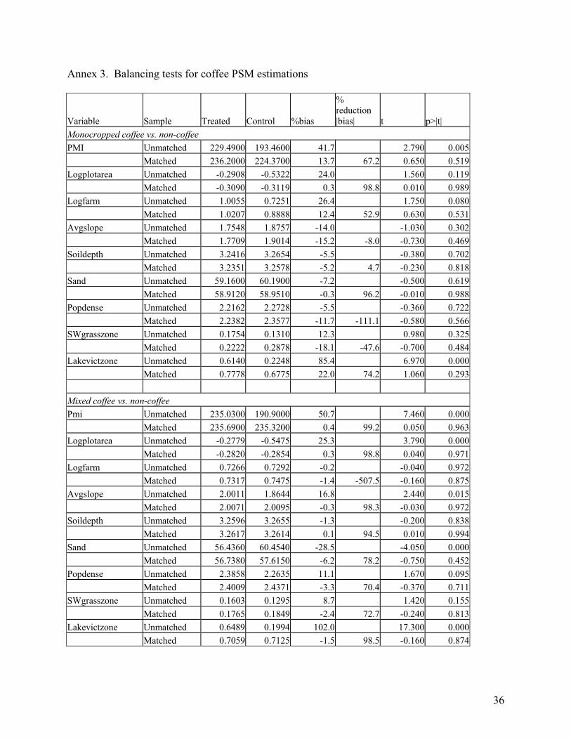
36
Annex 3. Balancing tests for coffee PSM estimations
Variable Sample Treated Control %bias
% reduction |bias| t p>|t|
Monocropped coffee vs. non-coffee PMI Unmatched 229.4900 193.4600 41.7 2.790 0.005 Matched 236.2000 224.3700 13.7 67.2 0.650 0.519Logplotarea Unmatched -0.2908 -0.5322 24.0 1.560 0.119 Matched -0.3090 -0.3119 0.3 98.8 0.010 0.989Logfarm Unmatched 1.0055 0.7251 26.4 1.750 0.080 Matched 1.0207 0.8888 12.4 52.9 0.630 0.531Avgslope Unmatched 1.7548 1.8757 -14.0 -1.030 0.302 Matched 1.7709 1.9014 -15.2 -8.0 -0.730 0.469Soildepth Unmatched 3.2416 3.2654 -5.5 -0.380 0.702 Matched 3.2351 3.2578 -5.2 4.7 -0.230 0.818Sand Unmatched 59.1600 60.1900 -7.2 -0.500 0.619 Matched 58.9120 58.9510 -0.3 96.2 -0.010 0.988Popdense Unmatched 2.2162 2.2728 -5.5 -0.360 0.722 Matched 2.2382 2.3577 -11.7 -111.1 -0.580 0.566SWgrasszone Unmatched 0.1754 0.1310 12.3 0.980 0.325 Matched 0.2222 0.2878 -18.1 -47.6 -0.700 0.484Lakevictzone Unmatched 0.6140 0.2248 85.4 6.970 0.000 Matched 0.7778 0.6775 22.0 74.2 1.060 0.293 Mixed coffee vs. non-coffee Pmi Unmatched 235.0300 190.9000 50.7 7.460 0.000 Matched 235.6900 235.3200 0.4 99.2 0.050 0.963Logplotarea Unmatched -0.2779 -0.5475 25.3 3.790 0.000 Matched -0.2820 -0.2854 0.3 98.8 0.040 0.971Logfarm Unmatched 0.7266 0.7292 -0.2 -0.040 0.972 Matched 0.7317 0.7475 -1.4 -507.5 -0.160 0.875Avgslope Unmatched 2.0011 1.8644 16.8 2.440 0.015 Matched 2.0071 2.0095 -0.3 98.3 -0.030 0.972Soildepth Unmatched 3.2596 3.2655 -1.3 -0.200 0.838 Matched 3.2617 3.2614 0.1 94.5 0.010 0.994Sand Unmatched 56.4360 60.4540 -28.5 -4.050 0.000 Matched 56.7380 57.6150 -6.2 78.2 -0.750 0.452Popdense Unmatched 2.3858 2.2635 11.1 1.670 0.095 Matched 2.4009 2.4371 -3.3 70.4 -0.370 0.711SWgrasszone Unmatched 0.1603 0.1295 8.7 1.420 0.155 Matched 0.1765 0.1849 -2.4 72.7 -0.240 0.813Lakevictzone Unmatched 0.6489 0.1994 102.0 17.300 0.000 Matched 0.7059 0.7125 -1.5 98.5 -0.160 0.874
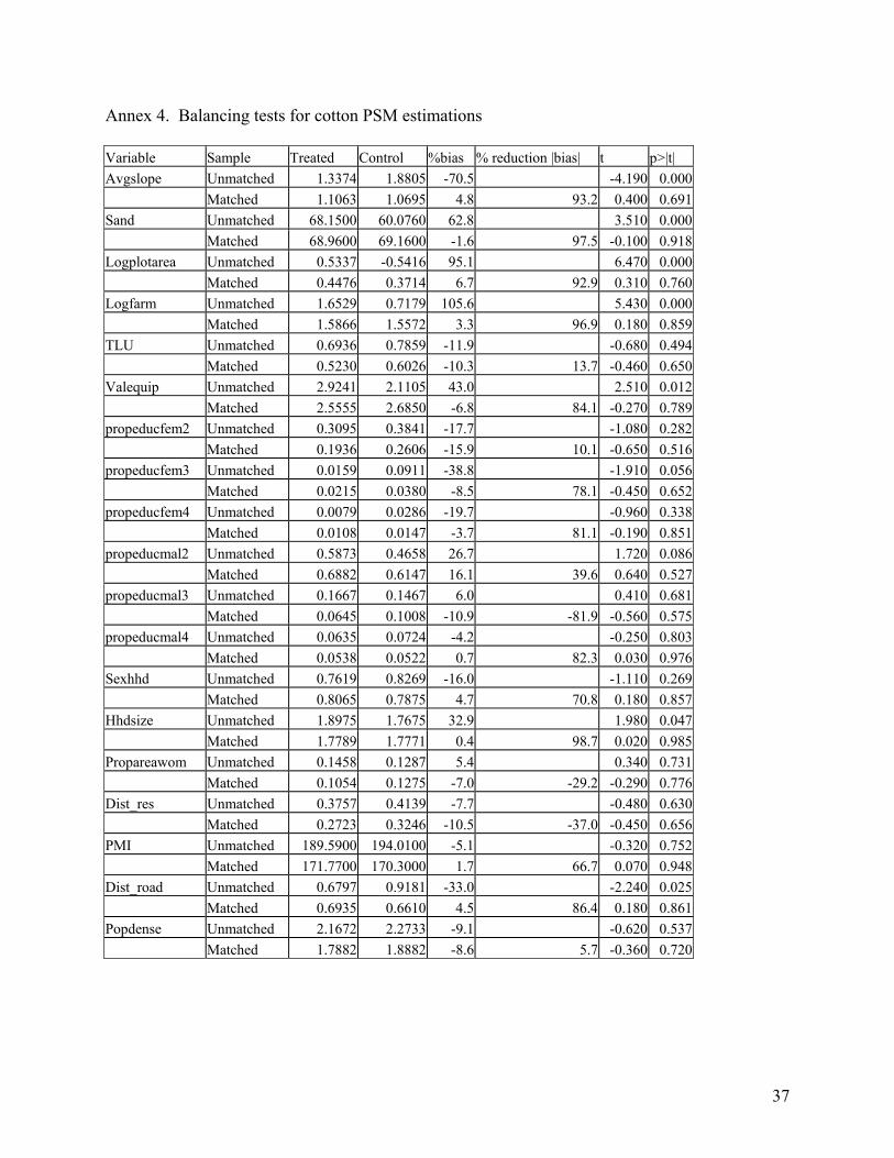
37
Annex 4. Balancing tests for cotton PSM estimations Variable Sample Treated Control %bias % reduction |bias| t p>|t| Avgslope Unmatched 1.3374 1.8805 -70.5 -4.190 0.000 Matched 1.1063 1.0695 4.8 93.2 0.400 0.691 Sand Unmatched 68.1500 60.0760 62.8 3.510 0.000 Matched 68.9600 69.1600 -1.6 97.5 -0.100 0.918 Logplotarea Unmatched 0.5337 -0.5416 95.1 6.470 0.000 Matched 0.4476 0.3714 6.7 92.9 0.310 0.760 Logfarm Unmatched 1.6529 0.7179 105.6 5.430 0.000 Matched 1.5866 1.5572 3.3 96.9 0.180 0.859 TLU Unmatched 0.6936 0.7859 -11.9 -0.680 0.494 Matched 0.5230 0.6026 -10.3 13.7 -0.460 0.650 Valequip Unmatched 2.9241 2.1105 43.0 2.510 0.012 Matched 2.5555 2.6850 -6.8 84.1 -0.270 0.789 propeducfem2 Unmatched 0.3095 0.3841 -17.7 -1.080 0.282 Matched 0.1936 0.2606 -15.9 10.1 -0.650 0.516 propeducfem3 Unmatched 0.0159 0.0911 -38.8 -1.910 0.056 Matched 0.0215 0.0380 -8.5 78.1 -0.450 0.652 propeducfem4 Unmatched 0.0079 0.0286 -19.7 -0.960 0.338 Matched 0.0108 0.0147 -3.7 81.1 -0.190 0.851 propeducmal2 Unmatched 0.5873 0.4658 26.7 1.720 0.086 Matched 0.6882 0.6147 16.1 39.6 0.640 0.527 propeducmal3 Unmatched 0.1667 0.1467 6.0 0.410 0.681 Matched 0.0645 0.1008 -10.9 -81.9 -0.560 0.575 propeducmal4 Unmatched 0.0635 0.0724 -4.2 -0.250 0.803 Matched 0.0538 0.0522 0.7 82.3 0.030 0.976 Sexhhd Unmatched 0.7619 0.8269 -16.0 -1.110 0.269 Matched 0.8065 0.7875 4.7 70.8 0.180 0.857 Hhdsize Unmatched 1.8975 1.7675 32.9 1.980 0.047 Matched 1.7789 1.7771 0.4 98.7 0.020 0.985 Propareawom Unmatched 0.1458 0.1287 5.4 0.340 0.731 Matched 0.1054 0.1275 -7.0 -29.2 -0.290 0.776 Dist_res Unmatched 0.3757 0.4139 -7.7 -0.480 0.630 Matched 0.2723 0.3246 -10.5 -37.0 -0.450 0.656 PMI Unmatched 189.5900 194.0100 -5.1 -0.320 0.752 Matched 171.7700 170.3000 1.7 66.7 0.070 0.948 Dist_road Unmatched 0.6797 0.9181 -33.0 -2.240 0.025 Matched 0.6935 0.6610 4.5 86.4 0.180 0.861 Popdense Unmatched 2.1672 2.2733 -9.1 -0.620 0.537 Matched 1.7882 1.8882 -8.6 5.7 -0.360 0.720