impact of use valuation of agricultural land: evidence from wisconsin

National Tax Association

IMPACT OF USE VALUATION OF AGRICULTURAL LAND: EVIDENCE FROM WISCONSINAuthor(s): Rebecca BoldtSource: Proceedings. Annual Conference on Taxation and Minutes of the Annual Meeting ofthe National Tax Association, Vol. 95 (2002), pp. 165-175Published by: National Tax AssociationStable URL: http://www.jstor.org/stable/41954281 .

Accessed: 12/06/2014 16:04

Your use of the JSTOR archive indicates your acceptance of the Terms & Conditions of Use, available at .http://www.jstor.org/page/info/about/policies/terms.jsp

.JSTOR is a not-for-profit service that helps scholars, researchers, and students discover, use, and build upon a wide range ofcontent in a trusted digital archive. We use information technology and tools to increase productivity and facilitate new formsof scholarship. For more information about JSTOR, please contact [email protected].

.

National Tax Association is collaborating with JSTOR to digitize, preserve and extend access to Proceedings.Annual Conference on Taxation and Minutes of the Annual Meeting of the National Tax Association.

http://www.jstor.org

This content downloaded from 185.2.32.96 on Thu, 12 Jun 2014 16:04:39 PMAll use subject to JSTOR Terms and Conditions

http://www.jstor.org/action/showPublisher?publisherCode=nta

http://www.jstor.org/stable/41954281?origin=JSTOR-pdf

http://www.jstor.org/page/info/about/policies/terms.jsp


IMPACT OF USE VALUATION OF AGRICULTURAL LAND: EVIDENCE FROM WISCONSIN

Rebecca Boldt, Wisconsin Department of Revenue*

The levels Wisconsin

effect and

of the is

use

the preservation valuation

subject of

on

this of property farmland paper. The

tax in levels and the preservation of farmland in

Wisconsin is the subject of this paper. The first section is a legislative history, followed by a discussion of the impact of use valuation on the taxable value of agricultural land and the resulting changes in property taxes. The next sections measure the effect of use valuation on farmland preservation and examine whether the property tax reductions under use valuation have been capitalized into higher agricultural land values.

LEGISLATIVE HISTORY The standard for assessment of agricultural land

in Wisconsin was changed in 1995 from full market value of the land to use value. Under use value, land devoted primarily to agriculture is assessed for property tax purposes on the basis of its net income generated from the land's rental for agricultural use.1 To mitigate drastic changes in assessments, use valuation was to be phased in over 10 years, beginning with a freeze in the assessed value for agricultural land in 1996 and 1997 at 1995 levels. The 1995 frozen assessed value of agricultural land was to be reduced each year by 10 percent of the difference between its frozen value and its use value. In 2000, the Department of Revenue promulgated emergency administrative rules that discontinued the remainder of the phase-in and began full implementation of use valuation.2 Shortly after enactment of the use value law, two lawsuits were filed challenging several as- pects of its implementation. The State Supreme Court eventually affirmed the law in June 2002.

IMPACT OF USE VALUATION ON ASSESSED VALUE AND PROPERTY TAXES

Data Sources Prior to the State Supreme Court's ruling, un-

certainty of the outcome of the lawsuits led the

*The author is with the Division of Research and Policy. This paper does not necessarily reflect the views of the Wisconsin Department of Revenue. The author is grateful for the valuable comments and assistance provided by Eng Braun and Dennis Collier.

Department of Revenue to continue collecting and analyzing market data in order to establish market-based assessments should the law be over- turned. As a result, data are available to measure with specificity what the value and property taxes on agricultural land would have been had market valuation continued to be the standard of assessment. The data revealed the extent to which use valuation has reduced taxable values and, in turn, the property taxes on agricultural land.

Chart 1 shows the use value of agricultural land from 1996-2002. As intended, the taxable value of agricultural land was relatively unchanged in the 1996-97 freeze period, but fell almost 10 percent in 1998, the first year of the phase-in. In 2000, the first year of full implementation, the taxable value of agricultural land fell over 32 percent from the prior year and approximately 44 percent from its value in 1995, the last year of market-based valuation. As a result of declining corn prices, the 2002 use value is estimated to be $2.8 billion, 45 percent lower than the 2001 values.

Comparison of Use Valuation to Market-Based Assessment

Agricultural land assessments and property taxes can be compared under use valuation and the market-based standard (see Chart 2). During the 1996-2002 period, assessments of agricultural land under a market-based assessment would have increased 12-18 percent annually. In contrast, agricultural land values under use value significantly declined over the period, particularly in 2000. Un- der full use value, the 2000 value of agriculture land was less than a third of its market-based assessment. The 2002 taxable value of agricultural land is expected to be $2.8 billion, which is 13.5 percent of its market-based assessment.

As a result of the declining use values during this period, agricultural land paid less in property taxes than it would have under a market-based assessment. Chart 3 compares net property taxes on agricultural land under use value and market-based assessment for the 1996-2002 period. Property tax savings on agricultural land under use value were 7-15 percent of market-based taxes during the

165



NATIONAL TAX ASSOCIATION PROCEEDINGS

Chart 1: Agricultural Land Value Under Use Value, 1996-2002

Source: Wisconsin Department of Revenue

Chart 2: Agricultural Land Valuation, 1996-2002 Use Value vs. Market Value ($ billions)


Chart 3: Agricultural Land Property Taxes ($ millions), 1996-2002 Use Value vs. Market Value

Source : Wisconsin Department of Revenue

166



95™ ANNUAL CONFERENCE ON TAXATION

1996-97 freeze period, between 28 percent and 38 percent during the 1998-99 phase-in period, and between 60 percent and 82 percent with full implementation of use value. The 2002 property tax per acre was $4.41 under use value, compared to $24. 10 with a market-based assessment. The cumulative savings in net agricultural land property taxes over the 1996-2002 period is estimated to be $767 million.3

THE EFFECT OF USE VALUATION ON FARMLAND PRESERVATION

Prior Studies Previous studies on farmland preservation

find that use value has a minimal impact on preserving farmland. Coughlin, Berry and Paut (1978) argue that property tax reductions have been much less effective on land use patterns than soil productivity or the demand for developable land. Malme (1993) argues that use valuation can, at best, slow development by making ownership of agricultural land less burdensome for those wishing to continue farming. Kolesar and Scholl (1972) argue that use valuation in New Jersey failed in its goal of preserving New Jersey open space, pointing to 365,000 acres of farmland sold in the 1960s since implementation of use value. A 1991 New York State study of farmland conversion argues that in high-growth areas, the preservation of farmland is transitory at best, and that significant tax reductions may encourage conversion to the extent that the tax savings significantly reduce holding costs for owners wishing to develop the land. Ferguson (1988) measures the rates of farmland conversion in four Virginia counties be- fore and after the adoption of use valuation by regressing the percentage of farm acreage on a trend variable. He finds no change in the conversion trends in the three counties closest to Washington DC, but finds a lower conversion trend in the most rural county. He concludes that use valuation is not enough, by itself, to slow farmland conversion in high-growth areas, but may help preserve farmland in areas less subject to development pressure.

In prior studies, no data existed as to the market-based assessments and property taxes of agricultural land under a use value regime. Tax savings from use valuation could only be estimated. As such, none of these studies were able to quan-

tify the relationship between the tax reductions under use value and farmland conservation. In contrast, the Wisconsin data provide actual, as opposed to estimated, tax reductions afforded under use value.

Farmland Conversion in Wisconsin Data also exist for the number of acres sold for

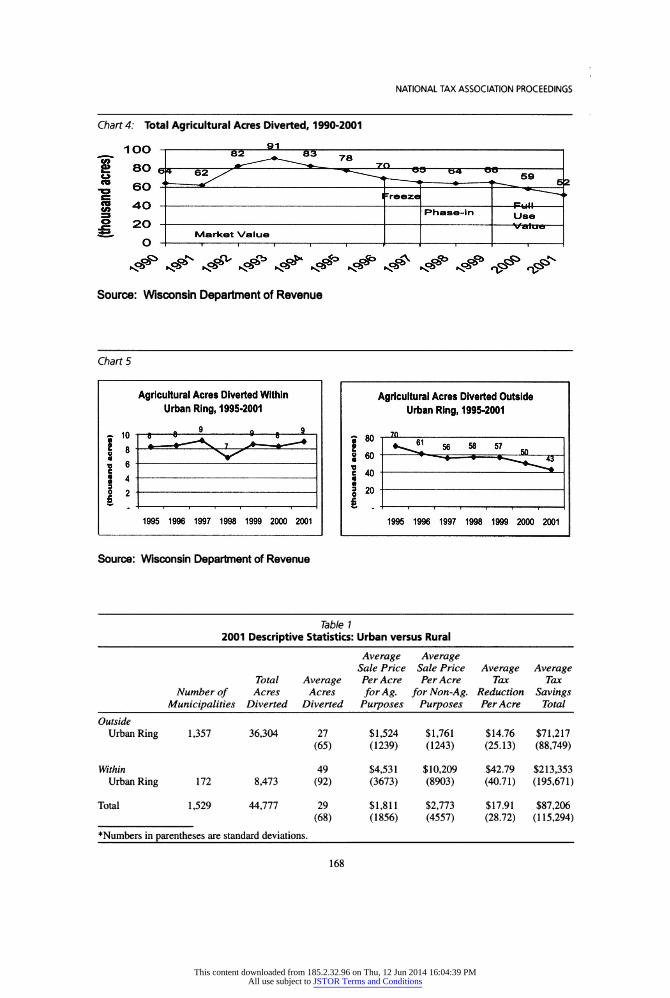
nonagricultural purposes, which provides a precise measure of farmland conversion.4 Chart 4 shows the number of acres diverted from agriculture in the five years prior to use value and the years since its implementation. The number of acres sold for non-agricultural purposes began to decline in 1993 and continued to decline into the 1998-99 phase-in years. Under full use value in 2000 and 2001, the acres sold for nonagricultural purposes declined 1 1 percent annually.

When the data are grouped by proximity to the urban fringe, the pace of conversion is markedly different. Municipalities are determined to be ei- ther within proximity to urban areas or in rural areas outside of urban influences.5 Chart 5 compares the farmland conversion in these two groups. Most municipalities are outside urban influences and therefore comprise around 90 percent of total agricultural acres in the state. In these municipalities, the annual conversion of agricultural acres declined by 12 percent and 14 percent in the two years under full use value (2000 and 2001). In contrast, conversion of agricultural acres in the urbanized municipalities have increased for the most part since 1998; by 2001, the same number of acres were diverted as in 1995, the last year of market valuation.

Table 1 reports 2001 descriptive statistics show- ing differences between urbanized and rural municipalities. The average 2001 tax reduction per acre under use value was around $15 in rural areas compared to $43 in urban areas. An average of 27 acres of agricultural land were diverted to nonagricultural purposes in rural areas compared to 49 acres in urban areas. To the extent that the urbanized areas saw the greatest tax reductions for agricultural land both in terms of total and per acre savings, the continued pace of farmland conversions in these areas suggests that use value has not been effective in preserving agricultural land most subject to development pressure. On the other hand, farmland conversion for the vast majority of agricultural land in the state has decreased since the implementation of use value.

167




Chart 4: Total Agricultural Acres Diverted, 1990-2001


Chart 5


Table 1 2001 Descriptive Statistics: Urban versus Rural

Average Average Sale Price Sale Price Average Average

Total Average Per Acre Per Acre Tax Tax Number of Acres Acres for Ag. for Non- Ag. Reduction Savings

Municipalities Diverted Diverted Purposes Purposes Per Acre Total Outside Urban Ring 1,357 36,304 27 $1,524 $1,761 $14.76 $71,217

(65) (1239) (1243) (25.13) (88,749)

Within 49 $4,531 $10,209 $42.79 $213,353 Urban Ring 172 8,473 (92) (3673) (8903) (40.71) (195,671)

Total 1,529 44,777 29 $1,811 $2,773 $17.91 $87,206 (68) (1856) (4557) (28.72) (115,294)

*Numbers in parentheses are standard deviations.

168




An Empirical Model of Farmland Preservation under Use Value

This section presents a model that relates the sale of agricultural land for nonagricultural purposes in each municipality to (1) the tax difference per acre under a market-based assessment and use valuation; (2) the difference in the average price of agricultural land sold for nonagricultural purposes and the average price of agricultural land sold for agricultural purposes; and (3) dummy variables capturing eight of the nine agricultural districts in the state.

This equation is denoted as

(1) A„ = ß0 + ßjtt + ßJi + ß/„ + ßR„ + ßJ*P„

where:

i = municipality containing agricultural land (n = 7677, approximately 1535 for each year)

t = year, 1997-2001 A = number of agricultural acres sold for nonag-

ricultural purposes T = tax difference per acre of farmland under

market assessment and use valuation (tax savings from use value)

P = difference between the average price per acre of agricultural land sold for nonagricultural purposes and the average price per acre of agricultural land sold that remains in agriculture

R. = dummy variable representing Wisconsin Agricultural Statistics Service Districts j, 7 = 2-9

ßl < 0 would indicate that an increase in the tax savings from use valuation would decrease farmland conversion to nonagricultural use. A quadratic specification captures rates of change and turning points. A negative sign for both ßl and ß2 would indicate that tax savings reduce farmland conversion at an increasing rate. Oppo- site signs of ß{ and ß2 ( e.g., ß, < 0 and ß2 > 0, or vice versa), would indicate that tax savings reduce (increase) farmland conversions at a decreasing (increasing) rate until, at some point, an additional dollar of tax savings causes a change in the direction of the tax effect on farmland conversions.

It can be expected that ßv the price coefficient, would have a positive value since Pi represents the real estate market potential for agricultural land in a municipality.6 Greater profits earned for land sold for development can be expected to induce more acreage to be diverted out of agriculture. The ßu coefficient measures the effect of the tax-price interaction variable. It can be expected that the tax effect will be different at different levels of the price premium. A positive ßn coefficient would indicate that the (negative) tax effect is offset by the price premium.

The base equation can be expanded to test whether the intercept is different for urbanized municipalities than for rural ones by using a dummy variable that takes the value of 1 for municipalities within the urban ring and 0 for rural municipalities. This equation is denoted as:

(2) A^ß^ß^ + ßJi + ßf+ßK,,

+ ßJ,*P, + ß<A

where:

!1 0 otherwise

if urban municipality

center i is within proximity of an

urban center 0 otherwise

A positive coefficient for the D variable would indicate that the number of acres converted out of agriculture is higher for more urbanized areas than more rural areas, independent of other factors.

A third variant assumes the intercepts are the same, but includes dummy variables to test whether the slopes of the variables are different (i.e., whether there is a difference in the effect of the tax and price variables on farmland conversion) between urban and rural areas:

(3) A = ß0 + ßjti + ßj- + ß,Pli+ ßRß + ßJ*P„

+ ßtPT,+ ßiP?,! + ß.PP»

+ /WA

If ßu and/or ßl5 are not equal to zero, the tax effect on farmland conversion can be assumed to be different for urban versus rural municipalities. Similarly, a non- zero ßl6 would suggest that there is an urban influence on the price effect.

169




The results of the three regressions are reported in Table 2. In Equation 1, which assumes no difference between municipalities, the estimated coefficient is negative and statistically significant. The positive ß2 coefficient indicates that tax savings reduces farmland conversion at a decreasing rate.7 The tax elasticity measured at the mean indicates that a 10 percent increase in the tax savings

under use value reduces the acres of farmland converted out of agriculture by 1 . 1 percent.

The price coefficient, ßv is positive as expected, confirming that higher price premiums for developable land will directly influence the acres diverted out of agriculture. The price elasticity measured at the mean indicates that a 10 percent increase in the difference between the price of land

Table 2 Regression Results (Equations 1-3)

Equation 1 Equation 2 Equation 3 No. of Observations 7677 7677 7677

R2 0.222 0.23 0.235 S 70.62 70.48 70.41 Independent Variable Description Symbol Coeff. Constant ß~ 27.851 28.048* 29.122*

(2.119) (2.196) (2.210) Tax Savings Per Acre ($) T ßL -.568* -.618* -.783*

(.070) (0.071) (.089) (Tax Savings Per Acre)2 T2 ß2 0.00079* .00087* .0011*

(000) (000) (.000) Price Difference Per Acre ($) P ß3 0.0013* 0.00062 -0.00087

(.001) (.001) (.001) Tax X Price ($) T*P ß12 .000039* 0.000041* .000067*

(000) (000) (.000)

North-Central District R ß4 -2.921 -3.252 -2.881 (3.072) (3.069) (3.061)

North-East District R ß5 -3.147 -2.784 -2.34 (3.905) (3.897) (3.898)

West-Central District R ß6 24.473 23.643* 24.700* (3.088) (3.083) (3.080)

Central District R ß7 -.615 -.458 0.322 (3.429) (3.422) (3.420)

East-Central District R ß8 2.822 .450 3.341 (3.251) (3.282) (3.258)

South-West District R ß9 43.552 43.673* 44.169* (3.308) (3.329) (3.299)

South-Central District R ß10 14.363 12.739* 15.671* (3.312) (3.322) (3.315)

South-East District R ßn 13.289* 9.334* 11.547* (4.280) (4.324) (4.302)

Urban Dummy - Intercept Shifter ß13 16.020* (2.941)

Urban Dummy - Slope Shifter D*T ß14 .544* (.132)

Urban Dummy - Slope Shifter D*T2 ß15 -.00092 (.000)

Urban Dummy - Slope Shifter D*P ß16 .003* (.001)

Urban Dummy - Slope Shifter d*j*p ß ̂ -.000046 (000) *Significant at the 95% level Dependent Variable: Agricultural acres sold for nonagricultural purposes, 1997-2001

170



95th ANNUAL CONFERENCE ON TAXATION

Table 2 (continued) Elasticity: Equations 1-3

Average Average Average Tax Savings Acres Price

Equation: zTax EPrice Per Acre Diverted Difference 1 All Municipalities -0.113 0.047 $11.52 34.4 $916

2 Rural Municipalities -0.165 0.007 $9.52 33.1 $636 Urbanized Municipalities -0.273 0.081 $27.61 44.4 $3,177

3 Rural Municipalities -0.207 0.012 $9.52 33.1 $636 Urbanized Municipalities 0.022 0.347 $27.61 AAA $3,177

sold for nonagricultural purposes and the price sold for agricultural purposes results in a 0.47 percent increase in the number of acres diverted out of agriculture.

The coefficients for four of the 8 regional dummy variables are statistically significant and positive. Three of the four regions are character- ized by areas of high growth and rapid urbaniza- tion.8 The fourth region is highly agricultural but also an area with rapid farmland conversion.

Equation 3 estimates the urban-rural differential in the tax and price effect. The slope shift coefficients for T and P are statistically different from zero, suggesting that both the tax and price effects on farmland conversion are different for urbanized versus rural municipalities. The tax elasticity for rural municipalities suggests that a 10 percent increase in tax savings under use value results in 2. 1 percent fewer acres diverted out of agriculture. In contrast, a 10 percent increase in tax savings in urban municipalities results in .2 percent more acres diverted out of agriculture.9

The price elasticity for rural municipalities suggests that a 10 percent increase in the price premium results in a negligible increase (.01 percent) in farmland conversions in rural municipalities.10 By comparison, a 10 percent increase in the price premium in urban areas results in a 3.5 percent increase in farmland conversions.

Thus, it can be argued that tax savings have a significant (negative) impact on farmland conversions in rural areas, whereas the price difference has a more significant (positive) impact on farmland conversions in urban areas. These findings are consistent with the previously cited studies-use valuation may encourage farmland preservation in rural areas, but has little effect in areas most subject to development pressure. In these areas, the high demand for developable land appears to out

weigh any tax incentive to preserve agricultural land.

The low R 2 for all equations suggests that other factors need to be taken into account when deter- mining farmland conversion patterns. Possible explanatory variables include farm income, the average age of farm operators, and the degree of land use planning in the area. Farm income can be expected to inversely affect farmland conversion, while age can be expected to directly affect the number of acres converted. Finally, the degree of land use planning at the county or local level would affect farmland conversions because areas with more up-to-date land use plans may have more strin- gent requirements for rezoning of agricultural land.

CAPITALIZATION OF PROPERTY TAXES The effect of the property tax reduction on the

agricultural sector depends, in large part, on the extent to which the lower taxes on land are capitalized into higher land values. Both theory and empirical research suggest that lower (higher) property taxes would be capitalized, at least to some extent, into higher (lower) agricultural land values. Fischel (2002) compares the property tax and selling price of homes in a high-tax municipality with physically identical homes in a low-tax municipality. He argues that the wealth position of buyers in the low-tax community is the same as buyers in the high-tax community to the extent that the lower property taxes are offset by higher mortgage payments associated with higher property values. Youngman (2002) argues that when higher property taxes result in lower housing prices, the property owner at the time of the tax increase bears the economic burden of the higher taxes because capitalization reduces the amount realized on the sale of the home. In contrast, it can be argued that

171




long-time property owners will enjoy the economic benefit of a tax decrease; they pay less in property taxes in the near term and will eventually realize a higher value when the property is sold. In this case, the economic burden will be borne by the first- time buyer who has the same costs of ownership but does not benefit from the capital gain associated with a higher selling price.

Pasour (1973) measures the capitalization of property taxes on farmland in North Carolina. The value of farmland is negatively related to the effective property tax rate, implying that the tax rate is capitalized to some extent into land values. Us- ing Pasour' s approach, the extent to which lower property taxes under use value have been capitalized into higher land values can be estimated using Wisconsin data on land sales and property tax rates. This is formalized as

(4) AGVALt. = ß^n{RATEt) + ß7AGSH{. + ßR..

where

i = municipality with agricultural land sold for agricultural purposes (n - 3948)

t = year, 1997-2001 AGVAL = average dollar per acre of agricultural

land sold for agricultural purposes RATE = effective property tax rate (i.e. taxes as

a percent of market value) AGSH = share of grade 1 acres (top quality

agricultural land) to total agricultural acres

R. = dummy variable representing Wisconsin Agricultural Statistic Service Districts

A negative ß] would indicate that higher (lower) property tax rates negatively (positively) affect land values. It can be expected that land value will increase as the quality of agricultural land increases, as measured by the share of total agricultural land that is grade 1 soil. Thus, ß2 can be expected to be positive. Regional dummies are included to capture regional variation in farmland value.

To test whether there is greater capitalization of property taxes on the urban fringe, equation (4) is modified to include the urban-rural dummy variable D (1 if urban, 0 if rural) as follows:

(5) AGVAL. = ftln (RATEt) + ß^GSH. +

+ ß3D*'n(RATEi) + ßRji

A statistically significant ß3 would indicate different rates of capitalization in urban areas as compared to rural ones. Following Pasour, a semi log form is used for the tax rate variable. Under this form, a given percentage change in the tax rate results in the same absolute change in land value.11 Thus, a 10 percent increase in the tax rate would result in a change in the land value equal to

(6) Ay = /^lnO + 10 percent).

where Ay equals the change in land value. The results of equations (4) and (5) are shown

in Table 3. As expected, the percentage of high quality soil to total agricultural acres positively influences the price of agricultural land as measured by the AGSH coefficient in both equations. Both equations also show that agricultural land value is heavily influenced by location as measured by the regional dummy coefficients.

The results for equation (4) yield a negative and statistically significant coefficient for the tax rate variable (jSj), implying that lower taxes are capitalized into higher land prices. Using the regression results, the following question can be explored: would land values have been lower under a market-based assessment as compared to the values observed under use valuation?

The data suggest that the effective tax rate would have been 1 35 percent higher under a market-based assessment compared to the rate under use value (1.6 percent compared to 0.68 percent). As shown in equation (6), the effect on land values of a 135 percent increase in the property tax rate can be estimated. Using the estimated ßx coefficient, such an increase in the property tax rate would result in a $156 decrease in land values.12 Thus, there is evidence to suggest that land values would have been $156 lower had land continued to be assessed under a market standard.

Full capitalization of a 135 percent increase in the tax rate can be determined as follows. The average farmland sold for agricultural purposes is $1,548 per acre. At an interest rate of 9 percent and property tax rate of 0.68 percent, the land must yield a return of $150 to be consistent with a market value of $1,548 [$1,548 = Return/(.09 + .0068)]. If the tax rate increases 135 percent from .68 percent to 1.6 percent and the annual return is $150 per acre, market value is reduced to $1,414 [$150/ (.09 + .016)]. Thus, full capitalization implies that

172




Table 3 Regression Results (Equations 4-5)

Equation 4 Equation 5 No. of Observations 3948 3948

R2 0.887 0.9 S 759.47 717.97 Independent Variable Description Symbol Coeff- Effective Property Tax Rate (log) In (Rate) ßj -183.369* -172.838*

(7.254) (6.874) Share of Grade 1 Acres to Total Agri. Acres AGSH ß2 145.885* 196.477*

(62.723) (59.340)

North-Central District R ß3 -120.787 -100.276 (46.606) (44.070)

North-East District R ß4 -10.79 17.882 (57.619) (54.486)

West-Central District R ß5 226.045* 193.151* (43.977) (41.602)

Central District R ß6 173.042* 198.956* (50.178) (47.452)

East-Central District R ß7 518.352* 348.383* (53.912) (51.567)

South-West District R ß8 266.319* 306.113* (47.460) (44.904)

South-Central District R ß9 306.113* 824.380* (44.904) (48.480)

South-East District R ß10 2868.115* 2384.006* (65.823) (66.117)

Urban Dummy - Slope Shifter D*ln(rate) ßn -190.936* (8.813) ♦Significant at the 95% level Dependent Variable: Average dollar of Wisconsin farmland sold for agricultural purposes 1997-2001 (observations with agricultural sales)

land values would have decreased $134 per acre [$1,548 - $1,414]. The regression analysis suggests that the tax decrease was more than fully capitalized into higher land prices.13

Results for equation (5) suggest that taxes are capitalized to a larger extent in urban areas than in rural areas. In rural areas, the market-based property tax rate would have been 125 percent higher than the effective rate under use value (1.6 percent compared to 0.71 percent). Such an increase would have, according to the analysis, resulted in land prices being $140 lower in rural areas.14 In contrast, the market-based rate in urban areas would have been 290 percent higher than the rate under use value (1.6 percent compared to 0.41 percent). The analysis suggests that such an increase in the tax rate would have resulted in a $495 decrease in land values in urban areas.15 By comparison, full capitalization would imply an increase in land values equal to $112 in rural areas and $401 in urban areas.16

Thus, the regression results provide evidence of significant capitalization of lower property taxes into higher land values in both rural and urban areas, but the impact is greater in urban areas.

Under full capitalization, the total cost of owning property (mortgage payments plus property taxes) should, over time, be the same whether under a market-based standard or a use-value standard. The question arises, however, whether the property tax relief afforded under use value dis- proportionately benefits long-time owners of farmland relative to first- time buyers. It can be argued that the increase in land values resulting from use value could price some buyers out of the market, particularly on the urban fringe where greater capitalization occurs and where the demand for nonagricultural land is strong. This may help explain why use value is not found to have a dramatic impact on farmland preservation, particularly on the urban fringe.

173




CONCLUSION Use value assessments have provided the most

property tax relief to agricultural land located in urban and suburban areas of the state. In the ab- sence of use valuation, agricultural land in these areas would have seen higher market assessments and hence higher market-based taxes compared to agricultural land in more rural areas. To the extent that use value was intended to address rising property taxes resulting from development pressure, this result is neither unexpected nor unintended. Even in highly agricultural areas that have not experi- enced the same development pressure, use value has significantly reduced agricultural property taxes compared to market-based assessment. State- wide, agricultural property taxes on land fell 32 percent in the first year under full use value. By 2002, use value taxes were 18 percent of what they would have been under a market-based assessment.

Our regression analysis suggests that use value has had a disparate effect on farmland preservation across municipalities. In rural areas, the tax savings afforded under use value have contributed to farmland preservation. In urban areas, however, there is little evidence that use value has preserved farmland most subject to development pressure in spite of the fact that use value has provided dra- matically more tax savings in these areas.

The analysis also suggests that the reduced property taxes under use value have been capitalized, to some extent, into higher land prices. Capitaliza- tion is found be greater in areas most subject to development pressure. To the extent that the cost of owning farmland is unchanged due to capitalization, the property tax relief under use value has been offset by higher land values. This may help explain why use valuation, by itself, has done little to stem the conversion of farmland on the urban fringe.

Notes 1 Net income is determined by subtracting expenses from the gross income generated from corn produc- tion. Gross income is determined for each county and soil type by the product of the five-year average corn yield and the five-year average Wisconsin corn price. Expenses are calculated as the sum of (1) the product of the five-year average corn yield for each county and the five-year average cost per bushel of corn and (2) return to management, assumed to equal 5 percent of gross income. Net income is capitalized by divid- ing it by the sum of (1) the five-year average interest

charged on a one-year adjustable rate mortgage for medium-sized agricultural loans and (2) the net full value property tax rate of each municipality. 2 The Department of Revenue was acting on the re- commendation of the Farmland Advisory Council established under the use value law to make recom- mendations to the department regarding use valuation.

3 It is estimated that 16 percent of the tax reduction was shifted to agricultural improvements that continue to be subject to market-based assessments. Taking the intra-sector shift into account, the cumulative tax reductions on the agricultural sector was $644 million.

4 The number of agricultural acres sold for nonagricultural purposes is a better measure of farmland conversion than changes in total agricultural acres, particularly in the initial years of use value implementation. Prior to use valuation, assessment classifications may not be particularly precise. With the advent of differential assessment for agricultural and nonagricultural property, classifications become important and therefore more precise. As a result, annual changes in total agricultural acres may reflect improved classifi- cation and not changes in use.

5 The urban ring is determined to be 30 miles around the center of Milwaukee, 15 miles around Madison and 5 to 10 miles around 15 major Wisconsin cities, depending on population. 6 Unlike the tax variable, the price variable does not capture a shadow price. It is meant more to capture what farm owners may perceive as the difference in sale prices between land sold for development and land remaining in agriculture. However, land remaining in agriculture may not be marketable for development and thus could never obtain the average sale price for converted acreage.

7 The different signs for the ßi and ß2 coefficients also indicate a turning point. However, since the turning point is found at a $338 tax saving per acre, which is 29 times higher than the average $1 1 .52 tax savings per acre, one can assume that the tax savings has a negative effect on farmland diversion for most levels of tax savings. 8 These regions include Hudson, a city within 30 miles of Minneapolis-St. Paul (West-Central), Madison (South-Central), and the greater Milwaukee metropoli- tan area (South-East).

9 The positive tax elasticity for urbanized areas is due to the positive coefficient for the T2 variable which indicates a turning point at a tax savings equal to $ 1 1 .88 per acre. Since the average tax savings per acre for urban municipalities is $27.61, the elasticity measured at the mean is positive. 10 The P coefficient is not statistically different from zero; however, the non-zero price elasticity is due to the statistically significant tax-price interaction term.

11 While a given percentage increase in the tax rate results in the same absolute change in land prices re- gardless of the level of the tax rate, a change in the tax

174



95th ANNUAL CONFERENCE ON TAXATION

rate will result in a smaller percentage change in land values, the higher the tax rate.

12 Determined by ß,ln(l + 1.353) where ßx is estimated to be -183.369.

13 However, a different discount rate would result in a different level of full capitalization. One could argue that land appreciation should be included, thereby increasing the full capitalization amount.

14 Determined by j3,ln(l + 1.254) where j3, is estimated to be -172.838.

15 Determined by (ß, + ß3)'n(l + 2.90) where /3, is estimated to be -172.838 and ß3 is estimated to be -190.936.

16 Based on a 9 percent interest rate, an average land value under of $1,331 and $3,576 for rural and urban areas respectively, effective rates under use value equal to .007 1 and .0041 for rural and urban areas respectively, and market rates equal to .016 for both rural and urban areas.

175



impact of use valuation of agricultural land: evidence from wisconsin

Documents