impact of temperature and temperature-change on … · impact of temperature and temperature-change...

MASTER-THESIS

Impact of Temperature and Temperature-Change on Range-Cameras

Accomplished at the Institute ofPhotogrammetry and Remote Sensing

Vienna University of Technology

Examiner: Univ.Prof. Dipl.-Ing. Dr.techn. Norbert PfeiferSupervisor: Projektass. Dipl.-Ing. Wilfried Karel

in cooperation with the Institute ofGeodesy and Geophysics

Vienna University of Technology

with support ofUniv.Prof. Dipl.-Ing. Dr.techn. Andreas Wieserand Univ.Ass. Dipl.-Ing. Stefan Lederbauer

byPhilipp Zachhuber

Eduard-Bach-Straße 2a4540 Bad Hall

Vienna, September 21st 2011 _____________________

Acknowledgements

I would like to thank all those People who made it possible for me to write this thesis:

Paul Berlinger from the “Institute of Applied Physics” for his advice and theconstruction of an Infra-red sensor.

Paul Brandl from the “Institute of Electrodynamics, Microwave and Circuit Engineering”(EMCE) for a very helpful introduction to the use of the Oscilloscope and for the supplyof other electrotechnical equipment.

Claudia Eder, Johannes Fabiankowitsch, Stefan Lederbauer and AndreasWieser from the “Institute of Geodesy and Geophysics” for their help and support fromordering and funding equipment over organising the measurement laboratory to the setup of the linux software for the CamCube and their involvement in various meetings.

Wilfried Karel, Norbert Pfeifer and Hans Thüminger from the “Instituteof Photogrammetry and Remote Sensing” (IPF) for their help with components, theIPF-Software and helpful discussions and pieces of advice.

Georg Ramer and Bernhard Zachhuber from the “Institute of Chemical Technologiesand Analytics” for placing their infrared-camera at my dispose.At this point I would like to thank the “Vienna University of Technology” for the great variety of institutes withutterly helpful staff.

Georg, Johanna D.G. and Ulrike for certain instruments, Franzi for proofreadingand the fourth floor and other residents of a famous student housing for making theyears there to such a great time. Especially Alex and Mimi deserve to be mentionedseparately for reasons they know.

Finally I should not forget Eva, Resi, Simon and all other mates from the universitywho provided a pleasant study-environment.

Mein besonderer Dank geht an meine Eltern, die mir das Studium ermöglicht haben undmich in jeder Hinsicht unterstützt haben.

ii

Abstract

The present master thesis deals with the various influences of temperature on rangecameras.

The influences on the measured data and on the electronics itself as well as the relationbetween integration time and internal temperature was investigated. Experiments werecarried out with permanent monitoring of the housing temperature or if available theinternal one was used.

Measured distances as well as amplitudes were found to be depending on temperaturewith increasing distances and decreasing amplitudes at higher temperatures. Moreoverthe sensor´s temperature of the SwissRanger 3000 was found to increase with longerintegration times.

A look at dark current in the sensors revealed a quadratic increase of the amplitudeswith temperature and a spatial dependence. Furthermore the stability of the sensor andthe camera housing was investigated and showed some room for improvements.

Zusammenfassung

Die vorliegende Masterarbeit behandelt unterschiedliche Einflüsse von Temperatur aufDistanzkameras.

Sowohl Einflüsse auf Messdaten und Elektronik wurden nebst dem Zusammenhangzwischen Integrationszeit und interner Temperatur untersucht. Dazu wurden Gehäuse-und interne Temperaturen durchgehend überwacht soweit dies möglich war.

Mit steigender Temperatur wurden größere Distanzen und kleinere Amplituden registriert.Eine höhere Sensortemperatur bei längerer Integrationszeit wurde beim SwissRanger 3000festgestellt.

Dunkelstrom im Sensor zeigte einen quadratischen Anstieg mit steigender Temperaturund auch eine Abhängigkeit von der Position des Pixels. Bei der Formstabilität desSensors selber und vor allem des Gehäuses wurde Raum für Verbesserungen ausgemacht.

iii

Contents

1 Introduction 11.1 Motivation . . . . . . . . . . . . . . . . . . . . . . . . . . . . . . . . . . . 11.2 Related Work . . . . . . . . . . . . . . . . . . . . . . . . . . . . . . . . . . 21.3 Aim of this Thesis . . . . . . . . . . . . . . . . . . . . . . . . . . . . . . . 3

2 Range Imaging Cameras 42.1 Functionality of Range Imaging Cameras . . . . . . . . . . . . . . . . . . 4

2.1.1 Time-of-Flight Measurement Principle . . . . . . . . . . . . . . . . 42.1.2 Phase-Difference Distance Measurement . . . . . . . . . . . . . . . 52.1.3 Implementation . . . . . . . . . . . . . . . . . . . . . . . . . . . . . 5

2.2 Range Imaging Cameras for Testing . . . . . . . . . . . . . . . . . . . . . 62.2.1 The Image Sensors . . . . . . . . . . . . . . . . . . . . . . . . . . . 62.2.2 The Illumination . . . . . . . . . . . . . . . . . . . . . . . . . . . . 82.2.3 The Cooling System . . . . . . . . . . . . . . . . . . . . . . . . . . 112.2.4 Overview of Features of the Cameras . . . . . . . . . . . . . . . . . 13

3 Considerations on Setup 143.1 Geometry of the Object Space . . . . . . . . . . . . . . . . . . . . . . . . . 14

3.1.1 Geometry of the Target . . . . . . . . . . . . . . . . . . . . . . . . 143.1.2 Target Distance . . . . . . . . . . . . . . . . . . . . . . . . . . . . . 15

3.2 Camera mounting . . . . . . . . . . . . . . . . . . . . . . . . . . . . . . . . 163.2.1 Temperature Tapping . . . . . . . . . . . . . . . . . . . . . . . . . 173.2.2 Camera Support . . . . . . . . . . . . . . . . . . . . . . . . . . . . 17

3.3 Ambient Light . . . . . . . . . . . . . . . . . . . . . . . . . . . . . . . . . 193.4 Ambient Temperature . . . . . . . . . . . . . . . . . . . . . . . . . . . . . 20

4 Methods 224.1 Data Acquisition . . . . . . . . . . . . . . . . . . . . . . . . . . . . . . . . 224.2 Experiments . . . . . . . . . . . . . . . . . . . . . . . . . . . . . . . . . . . 22

4.2.1 Determination of the Target positions . . . . . . . . . . . . . . . . 234.2.2 Differences in Dark Current distribution . . . . . . . . . . . . . . . 24

5 Results 25

iv

5.1 Influence on Measured Data . . . . . . . . . . . . . . . . . . . . . . . . . . 255.1.1 Permanence at Room Temperature . . . . . . . . . . . . . . . . . . 255.1.2 Influence on Distance . . . . . . . . . . . . . . . . . . . . . . . . . 285.1.3 Influence on Amplitude . . . . . . . . . . . . . . . . . . . . . . . . 32

5.2 Influence of the integration time on internal temperature . . . . . . . . . . 345.3 Influence of Temperature on the Electronics . . . . . . . . . . . . . . . . . 36

5.3.1 Dark Current in the Sensor . . . . . . . . . . . . . . . . . . . . . . 365.3.2 Geometric stability of the imaging sensor . . . . . . . . . . . . . . 395.3.3 Sensor-location dependence of dark current . . . . . . . . . . . . . 435.3.4 Influence on the active Illumination . . . . . . . . . . . . . . . . . 455.3.5 Frequency Stability of the Illumination . . . . . . . . . . . . . . . . 47

5.4 Summary of Results . . . . . . . . . . . . . . . . . . . . . . . . . . . . . . 50

6 Conclusion 516.1 Conclusions . . . . . . . . . . . . . . . . . . . . . . . . . . . . . . . . . . . 516.2 Temperature related recommendations for practical work . . . . . . . . . 526.3 Future Work . . . . . . . . . . . . . . . . . . . . . . . . . . . . . . . . . . 52

A Appendix 53A.1 Instruments used for Experiments . . . . . . . . . . . . . . . . . . . . . . 53

A.1.1 Devices for heating and cooling . . . . . . . . . . . . . . . . . . . . 53A.1.2 Temperature Loggers . . . . . . . . . . . . . . . . . . . . . . . . . . 54A.1.3 Instruments for Illumination Analysis . . . . . . . . . . . . . . . . 54

Bibliography 57

v

1 Introduction

1.1 Motivation

The initial motivation to write about Range Imaging Cameras (RIMs) was the possibilityto contribute to the enhancement of the navigation capabilities of the partly internalproject of a 4-wheel robot (Seekur Jr.) that is currently under active development at the“Institute of Geodesy and Geophysics”. This vehicle is used for developing and testingnavigation algorithms. One essential part of it, besides the GPS receivers and radioantennas, is a range-camera, the CamCube 2.0 from PMDtech (CamCube). This rangecamera is used for kinematic position determination. The final device should allow precisenavigation without further external guidance like a tracking total station.

It turned out that also the “Institute of Photogrammetry and Remote Sensing” (IPF)is connected to research around RIMs. They have the much smaller SwissRanger 3000(SR3000) and were investigating internal scattering effects at the beginning of this work.There might be a more detailed research in this thesis about the SR3000 simply becauseof the easier handling, quicker data processing and the fact that it is not as bulky andcan be brought to intended temperatures in a reasonable time. Nevertheless the mainexperiments were carried out with both cameras, of course.

The fact that the influences of temperature have not been thoroughly researched so farmade it very challenging to work on this topic. Statements like “Measurements are foundto be highly dependent on temperature, and on the illumination and reflectivity of theobjects.” (Pattinson, 2010) made it even more interesting to fill this gap. Pattinson alsostates that frequency-dependent calibration parameters would be no longer valid if thefrequency they are based on is no longer static because of dependence on temperature.

More encouraging statements were given by other researchers for example “... temperature-induced drifts of the distance measurement lead to significant errors.” (Kahlmann, 2007)and “It is a known fact that the depth measurement drifts with the camera’s temperature.It is yet to be properly investigated how this error behaves systematically with temperature.”(Rapp, 2007). Those drifts could be detected and the findings hopefully improve theunderstanding on this topic.

Finally I want to cite some more cognitions that even more directed my interest totemperature related investigations: “...temperature effects are one of the dominant

1

1 Introduction

influences in range imaging.” ... “... the reduction of uncontrolled temperature effectswill become more important” (Kahlmann, 2007)

1.2 Related Work

The first successful realisation of an all-solid-state 3D Time-of-Flight (ToF) range-camerais described in Lange (2000). Aside from hardware related chapters mostly focusing on theusability of different types of components also thermal effects like the diffusion of chargesand temperature-variable characteristics related to the control current of the illuminatingLEDs are mentioned. A recommendation for operating imagers at low temperaturesis given. In the succeeding publication by Lange and Seitz (2001) the focus is, amongothers subjects, kept on the power budget and thermal diffusion and thermal noise (darkcurrent).

Also an interesting work related to range-cameras and the importance of the dependenceof modulators on temperature was carried out by Heinol (2001). His work deals mostlywith new modulation concepts.

In the following time attention was drawn to the internal heating of instruments andto distance drifts as a consequence thereof (Luan, 2001) but also detailed investigationof influences on the electronics were carried out (e.g. Schneider (2003)). Later on agroup around Kahlmann started more detailed research on thermal effects (Kahlmann,Remondino, and Ingensand, 2006) which also plays a role in his dissertation (Kahlmann,2007) where he notes a higher distance reading at higher ambient temperatures andintroduces a constructional correction by an internal reference path which reduces thetemperature influence during the warming up phase down to around 20 %. Experimentssimilar to the ones carried out within my present work can be found in Kahlmann´sworks too but only ambient temperatures are used there which do not seem to be directlyrelated to effects in the recorded data. Nevertheless he uses a closed temperature cycleand different behaviour can be interpreted into the results.

Finally I must not forget to mention more recent researches like from Steiger, Felder, andWeiss (2008) or Pattinson (2010) with sections about various influences of temperature.Also the ongoing research on optoelectronic integrated circuits (OEICs) at the EMCE1

should be mentioned (e.g. the ongoing Thesis “Untersuchung eines Referenzkanals füreinen 3D Kamera Chip” by Michael Hofbauer or work by Zach, Davidovic, andZimmermann (2010))

1http://www.emce.tuwien.ac.at/en/index.htm

2

http://www.emce.tuwien.ac.at/en/index.htm

1 Introduction

1.3 Aim of this Thesis

The aim of this thesis is to further investigate thermal effects on RIMs. In contrast tothe publications mentioned before, the idea behind this work is to focus on effects causedby temperature only. That way a better understanding of the effect of internal, externaland other temperatures should be achieved. Sufficient experiments should back up thefindings and allow precise recommendations on the use of RIMs at certain temperaturesor changing environments.

Influences of the atmosphere´s temperature were found to be not relevant (Kahlmann,2007) in most cases and are not of interest for this work.

Especially the period of acclimatisation, due to changing ambient temperatures, is ofgreat interest because this is the period of major changes in the recorded data. Thebeginning of recording was also problematic to handle in other publications because ofsometimes erratic measurements after switching on the instrument.

Two different range cameras were available. A look at the components of those cameras istaken after an introduction into basic range imaging principles. The results are presentedafter the chapters on the set-up of the experiments and methods used. Finally, conclusionsare made and recommendations for future works are given.

3

2 Range Imaging Cameras

“A range image is a large collection of distance measurements from a knownreference coordinate system to surfacepoints on object(s) in a scene.”Besl (1988)

2.1 Functionality of Range Imaging Cameras

According to Besl (1988) Range Imaging Cameras belong to the category of field-of-view sensors as they deliver instantly a distance image of all visible points without anymovement of the sensor or any other part of the camera. It should be kept in mind thata representation of distances in a regular grid might be called range image regardless ofhow the data was collected which can be misleading.

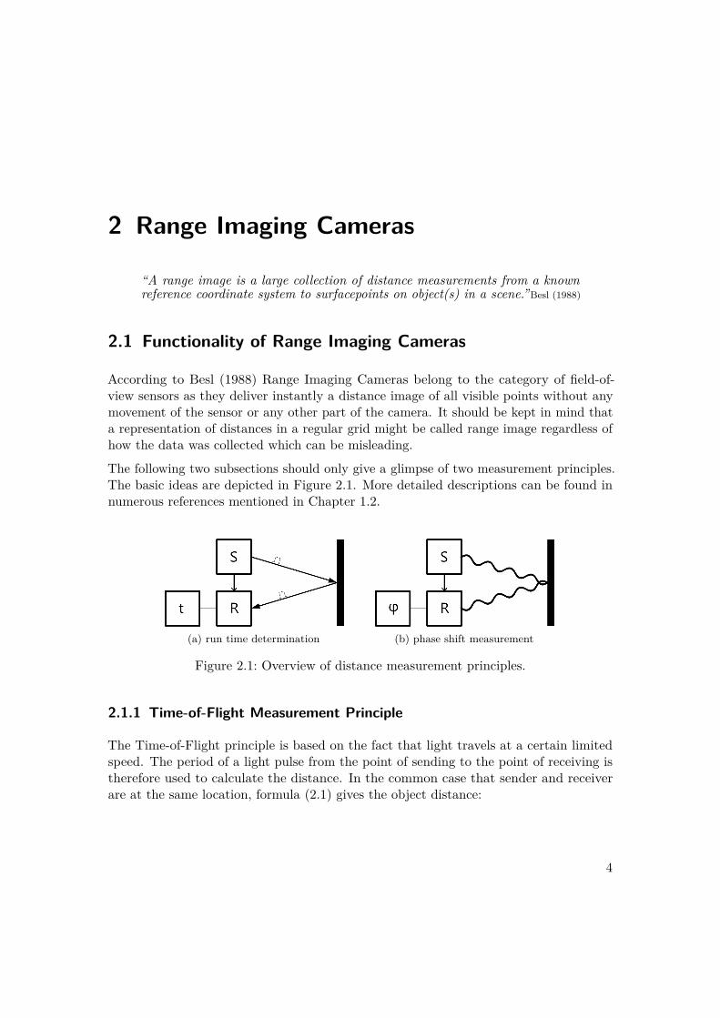
The following two subsections should only give a glimpse of two measurement principles.The basic ideas are depicted in Figure 2.1. More detailed descriptions can be found innumerous references mentioned in Chapter 1.2.

(a) run time determination (b) phase shift measurement

Figure 2.1: Overview of distance measurement principles.

2.1.1 Time-of-Flight Measurement Principle

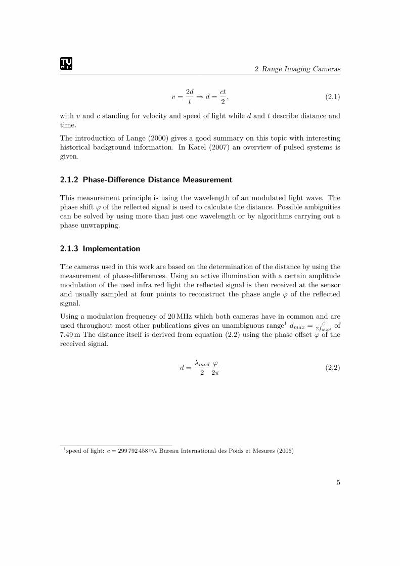
The Time-of-Flight principle is based on the fact that light travels at a certain limitedspeed. The period of a light pulse from the point of sending to the point of receiving istherefore used to calculate the distance. In the common case that sender and receiverare at the same location, formula (2.1) gives the object distance:

4


v = 2dt⇒ d = ct

2 , (2.1)

with v and c standing for velocity and speed of light while d and t describe distance andtime.

The introduction of Lange (2000) gives a good summary on this topic with interestinghistorical background information. In Karel (2007) an overview of pulsed systems isgiven.

2.1.2 Phase-Difference Distance Measurement

This measurement principle is using the wavelength of an modulated light wave. Thephase shift ϕ of the reflected signal is used to calculate the distance. Possible ambiguitiescan be solved by using more than just one wavelength or by algorithms carrying out aphase unwrapping.

2.1.3 Implementation

The cameras used in this work are based on the determination of the distance by using themeasurement of phase-differences. Using an active illumination with a certain amplitudemodulation of the used infra red light the reflected signal is then received at the sensorand usually sampled at four points to reconstruct the phase angle ϕ of the reflectedsignal.

Using a modulation frequency of 20MHz which both cameras have in common and areused throughout most other publications gives an unambiguous range1 dmax = c

2fmodof

7.49m The distance itself is derived from equation (2.2) using the phase offset ϕ of thereceived signal.

d = λmod

2ϕ

2π (2.2)

1speed of light: c = 299 792 458 m/s Bureau International des Poids et Mesures (2006)

5


2.2 Range Imaging Cameras for Testing

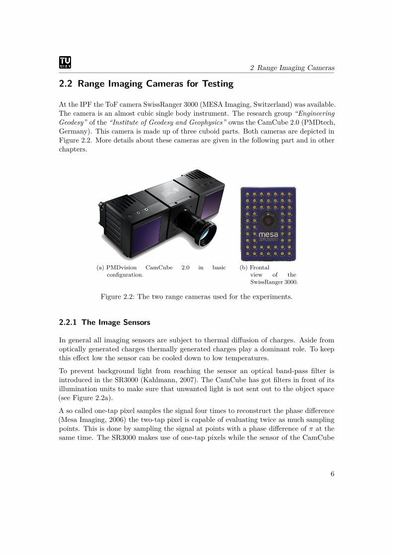
At the IPF the ToF camera SwissRanger 3000 (MESA Imaging, Switzerland) was available.The camera is an almost cubic single body instrument. The research group “EngineeringGeodesy” of the “Institute of Geodesy and Geophysics” owns the CamCube 2.0 (PMDtech,Germany). This camera is made up of three cuboid parts. Both cameras are depicted inFigure 2.2. More details about these cameras are given in the following part and in otherchapters.

(a) PMDvision CamCube 2.0 in basicconfiguration.

(b) Frontalview of theSwissRanger 3000.

Figure 2.2: The two range cameras used for the experiments.

2.2.1 The Image Sensors

In general all imaging sensors are subject to thermal diffusion of charges. Aside fromoptically generated charges thermally generated charges play a dominant role. To keepthis effect low the sensor can be cooled down to low temperatures.

To prevent background light from reaching the sensor an optical band-pass filter isintroduced in the SR3000 (Kahlmann, 2007). The CamCube has got filters in front of itsillumination units to make sure that unwanted light is not sent out to the object space(see Figure 2.2a).

A so called one-tap pixel samples the signal four times to reconstruct the phase difference(Mesa Imaging, 2006) the two-tap pixel is capable of evaluating twice as much samplingpoints. This is done by sampling the signal at points with a phase difference of π at thesame time. The SR3000 makes use of one-tap pixels while the sensor of the CamCube

6


uses two-tap pixels combined with averaging of the data. The distance and amplitude isderived from the sampling results in every single pixel.

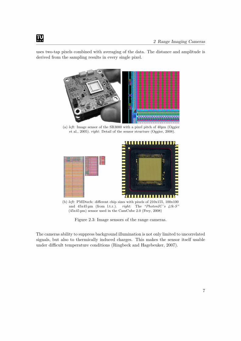
(a) left: Image sensor of the SR3000 with a pixel pitch of 40µm (Oggieret al., 2005). right: Detail of the sensor structure (Oggier, 2008).

(b) left: PMDtech: different chip sizes with pixels of 210x155, 100x100and 45x45µm (from l.t.r.). right: The “PhotonIC´s 41k-S”(45x45 µm) sensor used in the CamCube 2.0 (Frey, 2008)

Figure 2.3: Image sensors of the range cameras.

The cameras ability to suppress background illumination is not only limited to uncorrelatedsignals, but also to thermically induced charges. This makes the sensor itself usableunder difficult temperature conditions (Ringbeck and Hagebeuker, 2007).

7


2.2.2 The Illumination

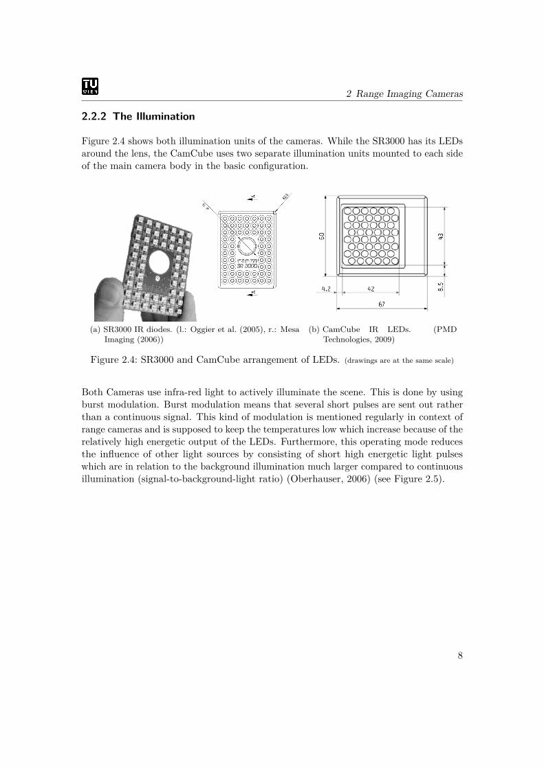
Figure 2.4 shows both illumination units of the cameras. While the SR3000 has its LEDsaround the lens, the CamCube uses two separate illumination units mounted to each sideof the main camera body in the basic configuration.

(a) SR3000 IR diodes. (l.: Oggier et al. (2005), r.: MesaImaging (2006))

(b) CamCube IR LEDs. (PMDTechnologies, 2009)

Figure 2.4: SR3000 and CamCube arrangement of LEDs. (drawings are at the same scale)

Both Cameras use infra-red light to actively illuminate the scene. This is done by usingburst modulation. Burst modulation means that several short pulses are sent out ratherthan a continuous signal. This kind of modulation is mentioned regularly in context ofrange cameras and is supposed to keep the temperatures low which increase because of therelatively high energetic output of the LEDs. Furthermore, this operating mode reducesthe influence of other light sources by consisting of short high energetic light pulseswhich are in relation to the background illumination much larger compared to continuousillumination (signal-to-background-light ratio) (Oberhauser, 2006) (see Figure 2.5).

8


Figure 2.5: Principle of burst-mode illumination (Oberhauser, 2006). Compared to thebackground light the burst modulation depicted right has a larger ratio ofthe signal. Between two bursts the LEDs have time to cool down a bit whichhelps to keep the temperatures low.

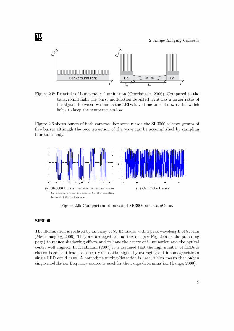
Figure 2.6 shows bursts of both cameras. For some reason the SR3000 releases groups offive bursts although the reconstruction of the wave can be accomplished by samplingfour times only.

(a) SR3000 bursts. (different Amplitudes caused

by aliasing effects introduced by the sampling

interval of the oscilloscope)

(b) CamCube bursts.

Figure 2.6: Comparison of bursts of SR3000 and CamCube.

SR3000

The illumination is realised by an array of 55 IR diodes with a peak wavelength of 850 nm(Mesa Imaging, 2006). They are arranged around the lens (see Fig. 2.4a on the precedingpage) to reduce shadowing effects and to have the centre of illumination and the opticalcentre well aligned. In Kahlmann (2007) it is assumed that the high number of LEDs ischosen because it leads to a nearly sinusoidal signal by averaging out inhomogeneities asingle LED could have. A homodyne mixing/detection is used, which means that only asingle modulation frequency source is used for the range determination (Lange, 2000).

9


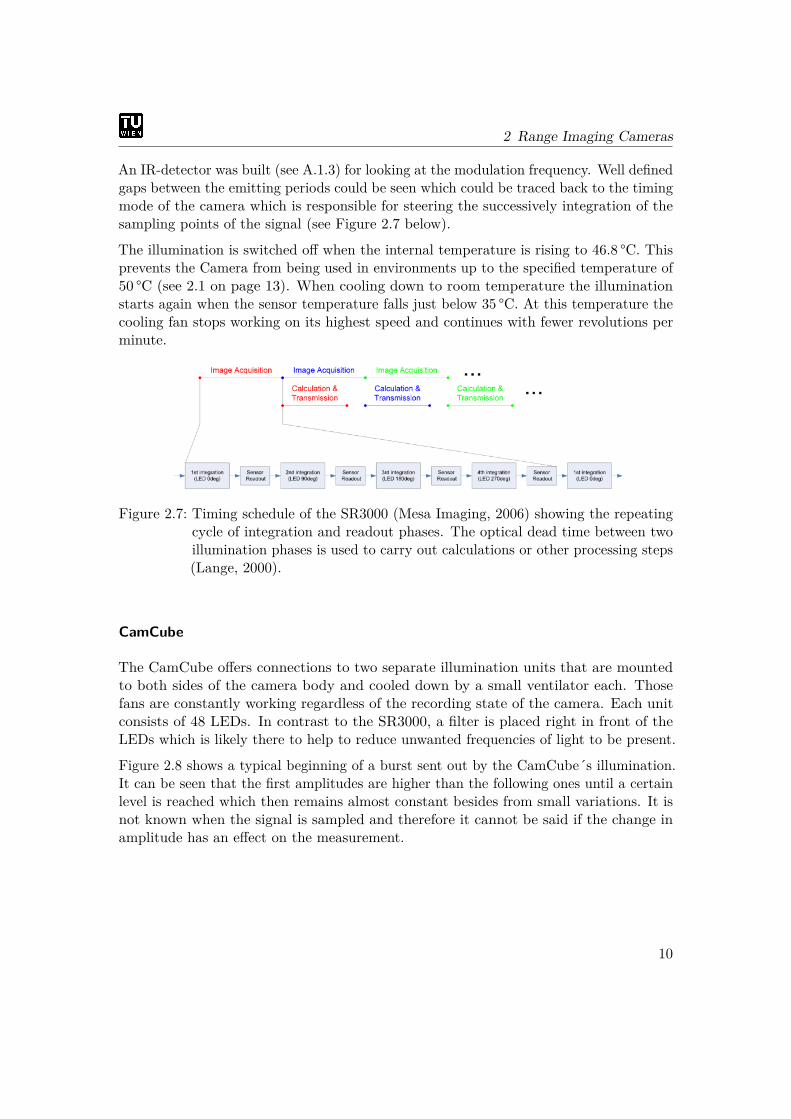
An IR-detector was built (see A.1.3) for looking at the modulation frequency. Well definedgaps between the emitting periods could be seen which could be traced back to the timingmode of the camera which is responsible for steering the successively integration of thesampling points of the signal (see Figure 2.7 below).

The illumination is switched off when the internal temperature is rising to 46.8 °C. Thisprevents the Camera from being used in environments up to the specified temperature of50 °C (see 2.1 on page 13). When cooling down to room temperature the illuminationstarts again when the sensor temperature falls just below 35 °C. At this temperature thecooling fan stops working on its highest speed and continues with fewer revolutions perminute.

Figure 2.7: Timing schedule of the SR3000 (Mesa Imaging, 2006) showing the repeatingcycle of integration and readout phases. The optical dead time between twoillumination phases is used to carry out calculations or other processing steps(Lange, 2000).

CamCube

The CamCube offers connections to two separate illumination units that are mountedto both sides of the camera body and cooled down by a small ventilator each. Thosefans are constantly working regardless of the recording state of the camera. Each unitconsists of 48 LEDs. In contrast to the SR3000, a filter is placed right in front of theLEDs which is likely there to help to reduce unwanted frequencies of light to be present.

Figure 2.8 shows a typical beginning of a burst sent out by the CamCube´s illumination.It can be seen that the first amplitudes are higher than the following ones until a certainlevel is reached which then remains almost constant besides from small variations. It isnot known when the signal is sampled and therefore it cannot be said if the change inamplitude has an effect on the measurement.

10


Figure 2.8: Detail of the first moments of a burst (CamCube).

2.2.3 The Cooling System

SR3000

Aside from the fact that the camera is temperature calibrated (mentioned in Oggier et al.(2005)) nothing is known about how this is done in detail.

The camera itself is cooled by a single ventilator that is driven at different speed levelsaccording to temperature. Air is blown through numerous vents on top and bottom ofthe housing. To allow proper cooling, the vents need to be kept free during all times. Forthis reason the camera was mounted as depicted in figure 2.9b (see chapter 3.2 “Cameramounting”).

11


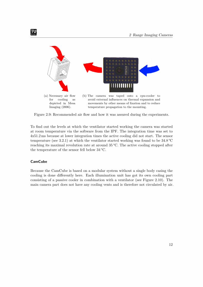
(a) Necessary air flowfor cooling asdepicted in MesaImaging (2006).

(b) The camera was taped onto a cpu-cooler toavoid external influences on thermal expansion andmovements by other means of fixation and to reducetemperature propagation to the mounting.

Figure 2.9: Recommended air flow and how it was assured during the experiments.

To find out the levels at which the ventilator started working the camera was startedat room temperature via the software from the IPF. The integration time was set to4x51.2ms because at lower integration times the active cooling did not start. The sensortemperature (see 3.2.1) at which the ventilator started working was found to be 34.8 °Creaching its maximal revolution rate at around 35 °C. The active cooling stopped afterthe temperature of the sensor fell below 34 °C.

CamCube

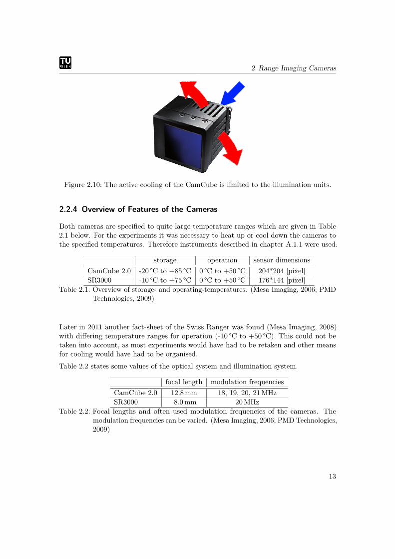
Because the CamCube is based on a modular system without a single body casing thecooling is done differently here. Each illumination unit has got its own cooling partconsisting of a passive cooler in combination with a ventilator (see Figure 2.10). Themain camera part does not have any cooling vents and is therefore not circulated by air.

12


Figure 2.10: The active cooling of the CamCube is limited to the illumination units.

2.2.4 Overview of Features of the Cameras

Both cameras are specified to quite large temperature ranges which are given in Table2.1 below. For the experiments it was necessary to heat up or cool down the cameras tothe specified temperatures. Therefore instruments described in chapter A.1.1 were used.

storage operation sensor dimensionsCamCube 2.0 -20 °C to +85 °C 0 °C to +50 °C 204*204 [pixel]SR3000 -10 °C to +75 °C 0 °C to +50 °C 176*144 [pixel]

Table 2.1: Overview of storage- and operating-temperatures. (Mesa Imaging, 2006; PMDTechnologies, 2009)

Later in 2011 another fact-sheet of the Swiss Ranger was found (Mesa Imaging, 2008)with differing temperature ranges for operation (-10 °C to +50 °C). This could not betaken into account, as most experiments would have had to be retaken and other meansfor cooling would have had to be organised.Table 2.2 states some values of the optical system and illumination system.

focal length modulation frequenciesCamCube 2.0 12.8mm 18, 19, 20, 21MHzSR3000 8.0mm 20MHz

Table 2.2: Focal lengths and often used modulation frequencies of the cameras. Themodulation frequencies can be varied. (Mesa Imaging, 2006; PMD Technologies,2009)

13

3 Considerations on Setup

All of the findings of the following subsections led to the final experimentation setup.The cameras were put on top of a metal plate supported by a surveying tripod. A flattarget with printed circles on it was about one meter away.

3.1 Geometry of the Object Space

3.1.1 Geometry of the Target

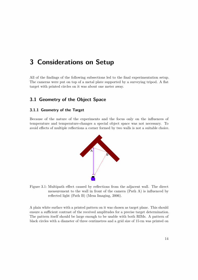
Because of the nature of the experiments and the focus only on the influences oftemperature and temperature-changes a special object space was not necessary. Toavoid effects of multiple reflections a corner formed by two walls is not a suitable choice.

Figure 3.1: Multipath effect caused by reflections from the adjacent wall. The directmeasurement to the wall in front of the camera (Path A) is influenced byreflected light (Path B) (Mesa Imaging, 2006).

A plain white surface with a printed pattern on it was chosen as target plane. This shouldensure a sufficient contrast of the received amplitudes for a precise target determination.The pattern itself should be large enough to be usable with both RIMs. A pattern ofblack circles with a diameter of three centimetres and a grid size of 15 cm was printed on

14


standard plotter paper. As stated in several publications standard office paper has veryhomogenous reflecting properties.

3.1.2 Target Distance

The basic idea of the setup is to keep things as simple as possible in order to concentrate ontemperature effects only. This leads to an arrangement that is close to the photogrammetricnormal case. This way effects of different angles of incidence by the illumination aremostly avoided.

The distance was kept relatively short with around one meter. This way the signal tonoise ratio should be high enough and not unnecessarily decreased by a too large distanceand then smaller amplitude. The influence of temperature should be seen regardless ofthe distance itself.

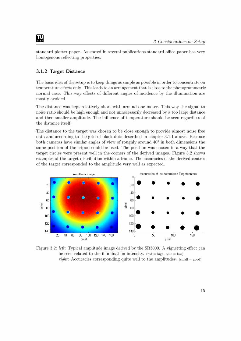
The distance to the target was chosen to be close enough to provide almost noise freedata and according to the grid of black dots described in chapter 3.1.1 above. Becauseboth cameras have similar angles of view of roughly around 40° in both dimensions thesame position of the tripod could be used. The position was chosen in a way that thetarget circles were present well in the corners of the derived images. Figure 3.2 showsexamples of the target distribution within a frame. The accuracies of the derived centresof the target corresponded to the amplitude very well as expected.

Figure 3.2: left: Typical amplitude image derived by the SR3000. A vignetting effect canbe seen related to the illumination intensity. (red = high, blue = low)right: Accuracies corresponding quite well to the amplitudes. (small = good)

15


3.2 Camera mounting

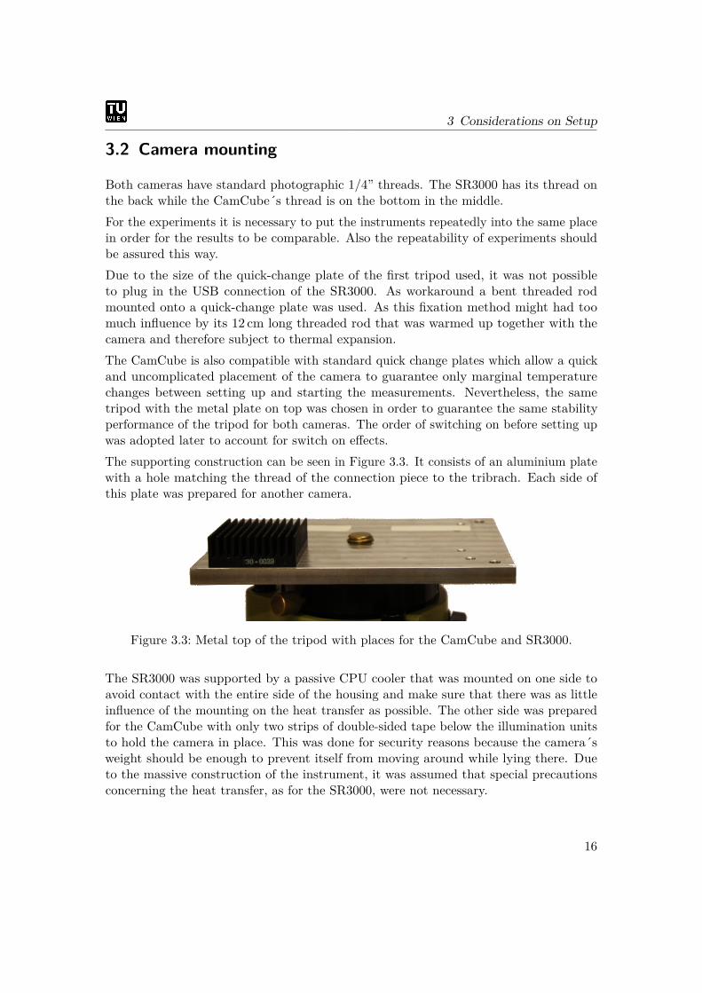
Both cameras have standard photographic 1/4” threads. The SR3000 has its thread onthe back while the CamCube´s thread is on the bottom in the middle.For the experiments it is necessary to put the instruments repeatedly into the same placein order for the results to be comparable. Also the repeatability of experiments shouldbe assured this way.Due to the size of the quick-change plate of the first tripod used, it was not possibleto plug in the USB connection of the SR3000. As workaround a bent threaded rodmounted onto a quick-change plate was used. As this fixation method might had toomuch influence by its 12 cm long threaded rod that was warmed up together with thecamera and therefore subject to thermal expansion.The CamCube is also compatible with standard quick change plates which allow a quickand uncomplicated placement of the camera to guarantee only marginal temperaturechanges between setting up and starting the measurements. Nevertheless, the sametripod with the metal plate on top was chosen in order to guarantee the same stabilityperformance of the tripod for both cameras. The order of switching on before setting upwas adopted later to account for switch on effects.The supporting construction can be seen in Figure 3.3. It consists of an aluminium platewith a hole matching the thread of the connection piece to the tribrach. Each side ofthis plate was prepared for another camera.

Figure 3.3: Metal top of the tripod with places for the CamCube and SR3000.

The SR3000 was supported by a passive CPU cooler that was mounted on one side toavoid contact with the entire side of the housing and make sure that there was as littleinfluence of the mounting on the heat transfer as possible. The other side was preparedfor the CamCube with only two strips of double-sided tape below the illumination unitsto hold the camera in place. This was done for security reasons because the camera´sweight should be enough to prevent itself from moving around while lying there. Dueto the massive construction of the instrument, it was assumed that special precautionsconcerning the heat transfer, as for the SR3000, were not necessary.

16


The depth of the metal plate was enough to support the various cable connections to thecameras so that no disturbing pulling force was able to come from there.

3.2.1 Temperature Tapping

A magnetic temperature probe (details in chapter A.1.2) was intended to monitor thehousing temperature of the cameras. Because the housing of the SR3000 is made ofaluminium it is not magnetic. Also the CamCube has a lack of reachable magnetic partsthat can be considered representative for the housing temperature. To solve this problem,little steel sheets were taped to the surface using a heat transfer compound to ensuregood contact and fairly accurate temperature measurements. Other advantages werethe quick mounting procedure of the thermal sensor without the use of fixing materialsand the perfectly repeatable sensor position. Figure 3.4 shows the CamCube with twodifferent positions of heat transferring metal sheets and the SR3000 with one on its side.

(a) Modified CamCube with thetemperature sampling pointindicated that was used duringthe experiments.

(b) Metalsheet fortemperaturetapping.

(c) SR3000 withtemperaturesampling on theside.

Figure 3.4: The range cameras with additional sheets of metal for better heat transfer.

Additional the temperature right next to the imaging sensor of the SR3000 could be readout with the IPF-software. This temperature was seen as identical with the temperatureof the sensor itself. It was not possible to read out an internal temperature of theCamCube and maybe such an internal sensor does not even exist.

3.2.2 Camera Support

To make sure that the tripod was steady enough an experiment was carried out using theSR3000 at room temperature. The aim of this experiment was to see if the position of thetarget points was constant or not. During a period of five hours the target pattern was

17


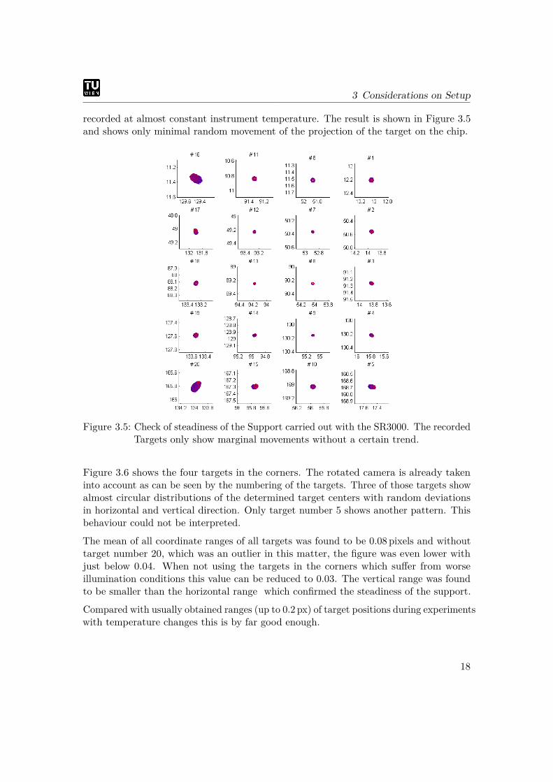
recorded at almost constant instrument temperature. The result is shown in Figure 3.5and shows only minimal random movement of the projection of the target on the chip.

Figure 3.5: Check of steadiness of the Support carried out with the SR3000. The recordedTargets only show marginal movements without a certain trend.

Figure 3.6 shows the four targets in the corners. The rotated camera is already takeninto account as can be seen by the numbering of the targets. Three of those targets showalmost circular distributions of the determined target centers with random deviationsin horizontal and vertical direction. Only target number 5 shows another pattern. Thisbehaviour could not be interpreted.

The mean of all coordinate ranges of all targets was found to be 0.08 pixels and withouttarget number 20, which was an outlier in this matter, the figure was even lower withjust below 0.04. When not using the targets in the corners which suffer from worseillumination conditions this value can be reduced to 0.03. The vertical range was foundto be smaller than the horizontal range which confirmed the steadiness of the support.

Compared with usually obtained ranges (up to 0.2 px) of target positions during experimentswith temperature changes this is by far good enough.

18


(a) target 16: 0.120 (b) target 01: 0.033

(c) target 20: 0.864 (d) target 5: 0.071

Figure 3.6: Targets recorded by the SR3000 during a 5 h long experiment. Corner targetsand their maximal coordinate range in pixels. Due to the low accuracy in thecorners those values represent upper limits.

3.3 Ambient Light

The influence of ambient light was investigated in a section in Pattinson (2010) and seenas negligible. Furthermore it was shown that detected frequencies that are even harmonicsof the modulation frequency do not have any influence on the distance measurementbecause of how the integration on the chip is done (Lange, 2000), possibly reducing theimpact of light sources which run on usual electrical outlets.

In the surveying laboratory that was used in this work fluorescent tubes are used forillumination as was the case in Pattinson (2010). Also actual research by Sajid Ghuffar

19


and Wilfried Karel did not entail any differences between measurements with lightseither turned on or off. Therefore it was no longer paid attention to the lighting situationbut nevertheless kept constant during the experiments.

3.4 Ambient Temperature

To see if a temperature variability in the measurement laboratory was present, athermometer was used to log this parameter.

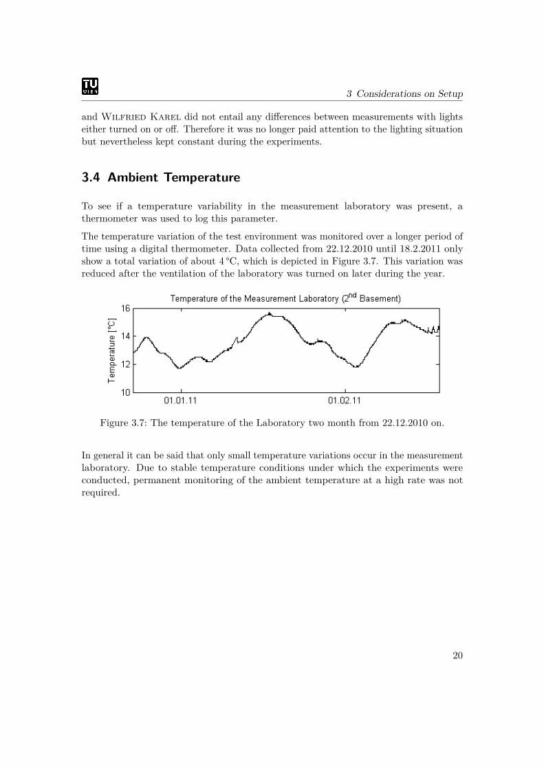
The temperature variation of the test environment was monitored over a longer period oftime using a digital thermometer. Data collected from 22.12.2010 until 18.2.2011 onlyshow a total variation of about 4 °C, which is depicted in Figure 3.7. This variation wasreduced after the ventilation of the laboratory was turned on later during the year.

Figure 3.7: The temperature of the Laboratory two month from 22.12.2010 on.

In general it can be said that only small temperature variations occur in the measurementlaboratory. Due to stable temperature conditions under which the experiments wereconducted, permanent monitoring of the ambient temperature at a high rate was notrequired.

20


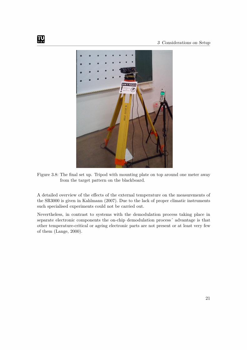
Figure 3.8: The final set up. Tripod with mounting plate on top around one meter awayfrom the target pattern on the blackboard.

A detailed overview of the effects of the external temperature on the measurements ofthe SR3000 is given in Kahlmann (2007). Due to the lack of proper climatic instrumentssuch specialised experiments could not be carried out.

Nevertheless, in contrast to systems with the demodulation process taking place inseparate electronic components the on-chip demodulation process´ advantage is thatother temperature-critical or ageing electronic parts are not present or at least very fewof them (Lange, 2000).

21

4 Methods

4.1 Data Acquisition

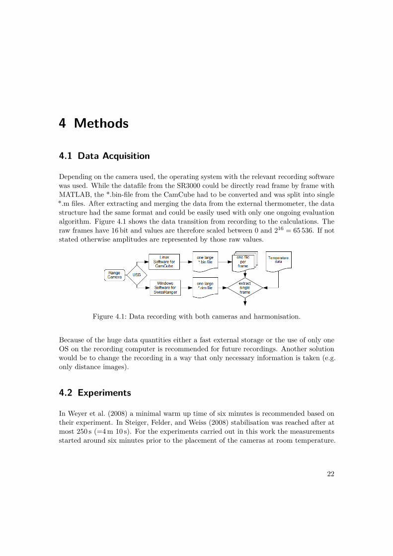
Depending on the camera used, the operating system with the relevant recording softwarewas used. While the datafile from the SR3000 could be directly read frame by frame withMATLAB, the *.bin-file from the CamCube had to be converted and was split into single*.m files. After extracting and merging the data from the external thermometer, the datastructure had the same format and could be easily used with only one ongoing evaluationalgorithm. Figure 4.1 shows the data transition from recording to the calculations. Theraw frames have 16 bit and values are therefore scaled between 0 and 216 = 65 536. If notstated otherwise amplitudes are represented by those raw values.

Figure 4.1: Data recording with both cameras and harmonisation.

Because of the huge data quantities either a fast external storage or the use of only oneOS on the recording computer is recommended for future recordings. Another solutionwould be to change the recording in a way that only necessary information is taken (e.g.only distance images).

4.2 Experiments

In Weyer et al. (2008) a minimal warm up time of six minutes is recommended based ontheir experiment. In Steiger, Felder, and Weiss (2008) stabilisation was reached after atmost 250 s (=4m 10 s). For the experiments carried out in this work the measurementsstarted around six minutes prior to the placement of the cameras at room temperature.

22

4 Methods

Because of separate ways of heating or cooling the cameras two runs were necessary mostof the time. Results were merged into a large dataset covering the whole temperaturerange according to Figure 4.2.

Figure 4.2: Merging of data from experiments.

4.2.1 Determination of the Target positions

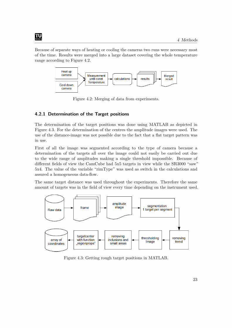
The determination of the target positions was done using MATLAB as depicted inFigure 4.3. For the determination of the centres the amplitude images were used. Theuse of the distance-image was not possible due to the fact that a flat target pattern wasin use.

First of all the image was segmented according to the type of camera because adetermination of the targets all over the image could not easily be carried out dueto the wide range of amplitudes making a single threshold impossible. Because ofdifferent fields of view the CamCube had 5x5 targets in view while the SR3000 “saw”5x4. The value of the variable “rimType” was used as switch in the calculations andassured a homogeneous data-flow.

The same target distance was used throughout the experiments. Therefore the sameamount of targets was in the field of view every time depending on the instrument used.

Figure 4.3: Getting rough target positions in MATLAB.

23

4 Methods

The derived rough target positions were used as an input parameter for more precisetarget calculations. Therefore a square area around the estimated position was usedas input parameter for the function "fitCumGauss" that was available at the IPF. Thisfunction uses a cumulated gaussian distribution as reference figure to describe circulartargets. This function uses a black image containing a white target. As the standardscaling delivers the inverse grey scale the negative had to be used. More details aredescribed in chapter “4.2.2. 2D Gaussian Distribution Fitting” in Otepka (2004). Thefitted target center as well as the accuracy of the center were used for the evaluation.

4.2.2 Differences in Dark Current distribution

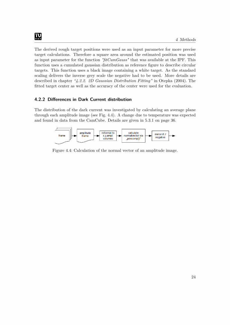
The distribution of the dark current was investigated by calculating an average planethrough each amplitude image (see Fig. 4.4). A change due to temperature was expectedand found in data from the CamCube. Details are given in 5.3.1 on page 36.

Figure 4.4: Calculation of the normal vector of an amplitude image.

24

5 Results

5.1 Influence on Measured DataThe target described in chapter 3.1.1 was used throughout the experiments.Most scatterplots in this chapter are based on the temperature and not on time and are colour-coded to ease the interpretation.

5.1.1 Permanence at Room Temperature

SR3000

A long time experiment carried out by Wilfried Karel was used to additionallymonitor the temperature of the instrument itself. In this experiment the SR3000 wasused to record a black surface for a period of several hours.The temperature of the housing was found to be constant aside from variations in theorder of the thermometer´s accuracy. The internal temperature (next to the sensor see.3.2.1) varied at most 0.74 °C but mainly only by 0.49 °C. Other long term experimentsshowed similar results.Looking at the sensor temperature of the 5 h-experiment used already in chapter 3.2.2revealed a periodic change of the internal temperature of around 1 °C at a frequency ofabout 25 s. Distances and amplitudes were found to change at the same rate which isconsistent with the findings of Karel, Ghuffar, and Pfeifer (2010).

CamCube

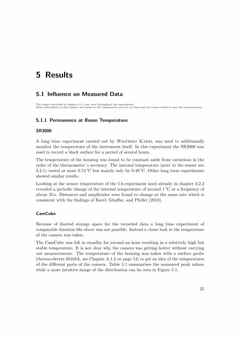
Because of limited storage space for the recorded data a long time experiment ofcomparable duration like above was not possible. Instead a closer look at the temperatureof the camera was taken.The CamCube was left in standby for around an hour resulting in a relatively high butstable temperature. It is not clear why the camera was getting hotter without carryingout measurements. The temperature of the housing was taken with a surface probe(thermo-electra 80102A, see Chapter A.1.2 on page 54) to get an idea of the temperaturesof the different parts of the camera. Table 5.1 summarises the measured peak values,while a more intuitive image of the distribution can be seen in Figure 5.1.

25

5 Results

part of the camera min. max.overall 23.7 27.7Camera 26.7 27.7

Illumination 23.7 25.8Table 5.1: Maximal and minimal temperatures measured at the CamCube while on

standby in [°C].

It was noticed that both illumination units had quite similar or rather almost identicalheat distributions. The passive cooling elements ventilated by a fan were rather cool,while only the more massive parts and areas with poor air flow heated up to around25.7 °C.

The camera itself did not heat up uniformly but up on one side more than on the other.This might be an effect caused by the fact that on the warmer side the electrical powerenters the instrument. A more detailed investigation if this temperature gradient wasrelated to the specific dark current distribution can be found in chapter 5.3.1.

Because of a small gap to the central camera cube the heat transfer amongst the differentparts was limited as Figure 5.1 suggests.

26

5 Resultsevery accessible face of each cube was sampled at nine points as indicated below

(a) Front view of the CamCube.

(b) Back view of the CamCube.

Figure 5.1: Qualitative temperature distribution of the CamCube in standby afterreaching a steady state.

27

5 Results

5.1.2 Influence on Distance

SR3000

As described before, two different temperature sampling places were available. Namely thetemperature of the sensor itself and the temperature of the housing. Several effects wereobserved when looking at the distances. The results depicted in Figure 5.4 were derivedfrom data collected at two consecutive days and merged as described in Chapter 4.2on page 22. The difference in the distance of around one centimetre between bothconstant states (the two clusters where the experiments meet in the Figure below) of theexperiments can not be explained definitely.

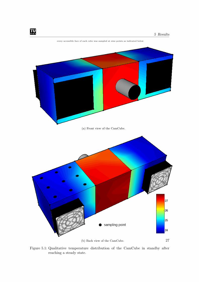
Looking at the diagram about the relation between the sensor temperature and thedistance in Figure 5.2 gives a hint of a hysteresis that might occur if the whole cycle iscarried out at once. A linear fit of the warm-up phase gives 1.4mm/°C while the fit ofthe cooling-down part gives around 2.1mm/°C.

Figure 5.2: left: Sensortemperature versus distance. middle: sensortemperature versusstandard deviation of the distance of a single frame. right: same as middlebut with the mean of 10 frames as reference.

The relation between the temperature of the sensor and the standard deviation of asingle distance-frame image gave a gradient of 0.72mm/°C in the cold part (withoutventilation) and 0.52mm/°C in the warm part (with ventilation).

Using 10 frames as reference, the standard deviation of the difference of the actual andthe reference frame showed a linear dependence from 16.8 to 18.9mm aside from outliersthat were mostly present around the already mentioned range of unsteady operationof the ventilation. A robust linear fit resulted in gradients of 0.038mm/°C (cold) and0.027mm/°C (warm).

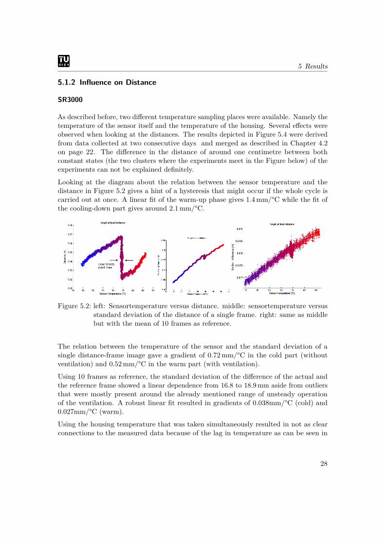
Using the housing temperature that was taken simultaneously resulted in not as clearconnections to the measured data because of the lag in temperature as can be seen in

28

5 Results

Figure 5.3. Those results were not further investigated but show the difference that couldbe introduced by using housing temperatures only. The differences are explained moreexactly later in this chapter.

Figure 5.3: Housingtemperature versus distance and housingtemperature versus thestandard deviation of the distance.

Looking at Figure 3.42 on page 84 of Kahlmann (2007)1, some basic similarities mightbe interpreted but those are too vague to be mentioned here. Because of the closedtemperature cycle used in that publication some differences between the warming andcooling can be detected as expected. However this was not the main focus although itmight be of interest for further investigations.

1only external temperatures are used in that work

29

5 Results

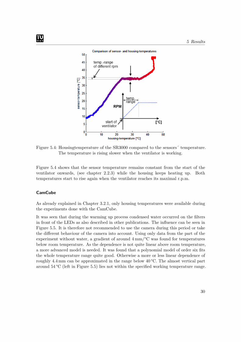
Figure 5.4: Housingtemperature of the SR3000 compared to the sensors´ temperature.The temperature is rising slower when the ventilator is working.

Figure 5.4 shows that the sensor temperature remains constant from the start of theventilator onwards, (see chapter 2.2.3) while the housing keeps heating up. Bothtemperatures start to rise again when the ventilator reaches its maximal r.p.m.

CamCube

As already explained in Chapter 3.2.1, only housing temperatures were available duringthe experiments done with the CamCube.

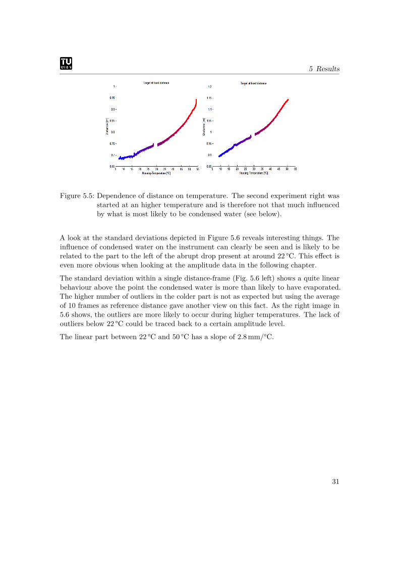
It was seen that during the warming up process condensed water occurred on the filtersin front of the LEDs as also described in other publications. The influence can be seen inFigure 5.5. It is therefore not recommended to use the camera during this period or takethe different behaviour of the camera into account. Using only data from the part of theexperiment without water, a gradient of around 4mm/°C was found for temperaturesbelow room temperature. As the dependence is not quite linear above room temperature,a more advanced model is needed. It was found that a polynomial model of order six fitsthe whole temperature range quite good. Otherwise a more or less linear dependence ofroughly 4.4mm can be approximated in the range below 40 °C. The almost vertical partaround 54 °C (left in Figure 5.5) lies not within the specified working temperature range.

30

5 Results

Figure 5.5: Dependence of distance on temperature. The second experiment right wasstarted at an higher temperature and is therefore not that much influencedby what is most likely to be condensed water (see below).

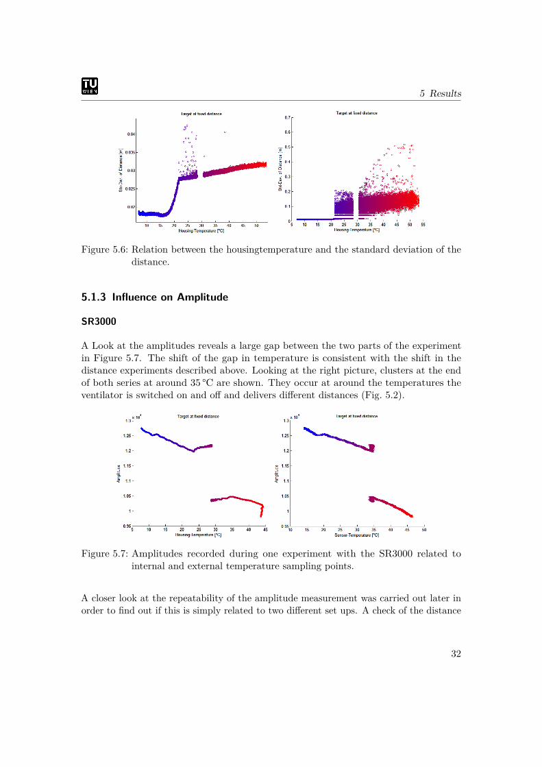
A look at the standard deviations depicted in Figure 5.6 reveals interesting things. Theinfluence of condensed water on the instrument can clearly be seen and is likely to berelated to the part to the left of the abrupt drop present at around 22 °C. This effect iseven more obvious when looking at the amplitude data in the following chapter.

The standard deviation within a single distance-frame (Fig. 5.6 left) shows a quite linearbehaviour above the point the condensed water is more than likely to have evaporated.The higher number of outliers in the colder part is not as expected but using the averageof 10 frames as reference distance gave another view on this fact. As the right image in5.6 shows, the outliers are more likely to occur during higher temperatures. The lack ofoutliers below 22 °C could be traced back to a certain amplitude level.

The linear part between 22 °C and 50 °C has a slope of 2.8mm/°C.

31

5 Results

Figure 5.6: Relation between the housingtemperature and the standard deviation of thedistance.

5.1.3 Influence on Amplitude

SR3000

A Look at the amplitudes reveals a large gap between the two parts of the experimentin Figure 5.7. The shift of the gap in temperature is consistent with the shift in thedistance experiments described above. Looking at the right picture, clusters at the endof both series at around 35 °C are shown. They occur at around the temperatures theventilator is switched on and off and delivers different distances (Fig. 5.2).

Figure 5.7: Amplitudes recorded during one experiment with the SR3000 related tointernal and external temperature sampling points.

A closer look at the repeatability of the amplitude measurement was carried out later inorder to find out if this is simply related to two different set ups. A check of the distance

32

5 Results

resulted in a mean difference of around 0.8mm. The comparison of the raw-amplitudesshowed only a deviation of -2.5 and for this reason the large gap above can not beexplained sufficiently.

CamCube

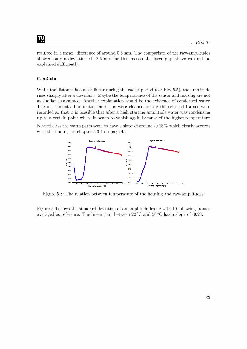
While the distance is almost linear during the cooler period (see Fig. 5.5), the amplituderises sharply after a downfall. Maybe the temperatures of the sensor and housing are notas similar as assumed. Another explanation would be the existence of condensed water.The instruments illumination and lens were cleaned before the selected frames wererecorded so that it is possible that after a high starting amplitude water was condensingup to a certain point where it began to vanish again because of the higher temperature.

Nevertheless the warm parts seem to have a slope of around -0.18% which closely accordswith the findings of chapter 5.3.4 on page 45.

Figure 5.8: The relation between temperature of the housing and raw-amplitudes.

Figure 5.9 shows the standard deviation of an amplitude-frame with 10 following framesaveraged as reference. The linear part between 22 °C and 50 °C has a slope of -0.23.

33

5 Results

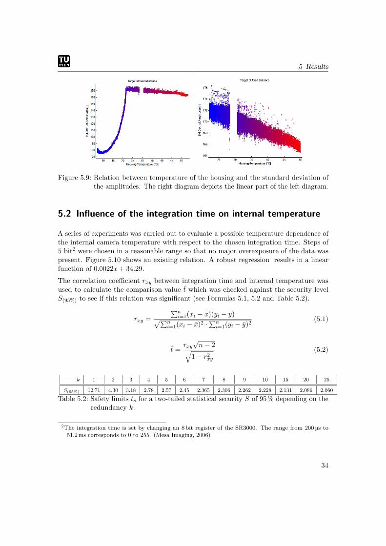
Figure 5.9: Relation between temperature of the housing and the standard deviation ofthe amplitudes. The right diagram depicts the linear part of the left diagram.

5.2 Influence of the integration time on internal temperature

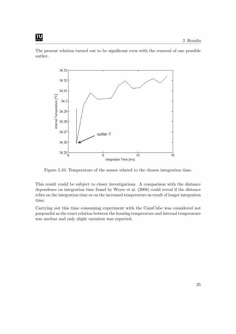
A series of experiments was carried out to evaluate a possible temperature dependence ofthe internal camera temperature with respect to the chosen integration time. Steps of5 bit2 were chosen in a reasonable range so that no major overexposure of the data waspresent. Figure 5.10 shows an existing relation. A robust regression results in a linearfunction of 0.0022x+ 34.29.The correlation coefficient rxy between integration time and internal temperature wasused to calculate the comparison value t which was checked against the security levelS(95%) to see if this relation was significant (see Formulas 5.1, 5.2 and Table 5.2).

rxy =∑n

i=1(xi − x)(yi − y)√∑ni=1(xi − x)2 ·

∑ni=1(yi − y)2 (5.1)

t = rxy

√n− 2√

1− r2xy

(5.2)

k 1 2 3 4 5 6 7 8 9 10 15 20 25

S(95%) 12.71 4.30 3.18 2.78 2.57 2.45 2.365 2.306 2.262 2.228 2.131 2.086 2.060Table 5.2: Safety limits ts for a two-tailed statistical security S of 95% depending on the

redundancy k.

2The integration time is set by changing an 8 bit register of the SR3000. The range from 200 µs to51.2ms corresponds to 0 to 255. (Mesa Imaging, 2006)

34

5 Results

The present relation turned out to be significant even with the removal of one possibleoutlier.

Figure 5.10: Temperature of the sensor related to the chosen integration time.

This result could be subject to closer investigations. A comparison with the distancedependence on integration time found by Weyer et al. (2008) could reveal if the distancerelies on the integration time or on the increased temperature as result of longer integrationtime.

Carrying out this time consuming experiment with the CamCube was considered notpurposeful as the exact relation between the housing temperature and internal temperaturewas unclear and only slight variation was expected.

35

5 Results

5.3 Influence of Temperature on the Electronics

5.3.1 Dark Current in the Sensor

Following chapter “4.2 Noise limitation of range accuracy” in Lange (2000) the rangeresolution ∆L of a four tap demodulation system is:

∆L = L

8 ·√B +Npseudo

2 ·A (5.3)

• L: Non-ambiguity distance

• A: Demodulation amplitude

• B: Acquired optical mean value

• Npseudo: Additional induced electrons

The presence of temperature generates electrons (dark current) that cannot be distinguishedfrom optically created ones. Therefore they are integrated the same way. It was now ofinterest to see if the dark current was evenly distributed within the sensor or not.

Experiments with covered lens to prevent external light to enter the system were carriedout. The illumination was covered to make sure that modulated light could not bedetected.

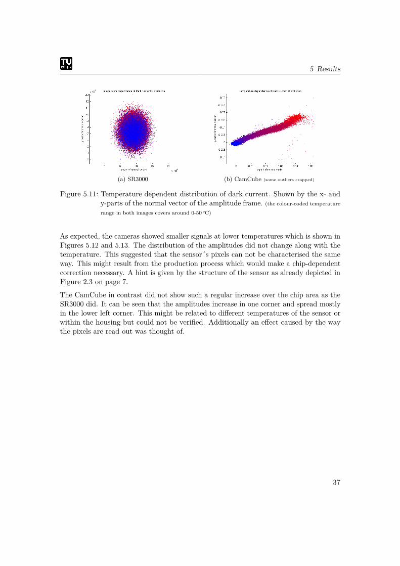
The single steps to the results depicted in Figure 5.11 can be found in Chapter 4.2.2on page 24. The images show that the distribution of the dark current is not equalthroughout the sensor. The x and y-parts of the normal vector were calculated fromamplitude images and the corresponding adjusted planes. While the SR3000 showsmostly constant proportions in both directions with only slight changes, the two partsof the CamCube show an obvious change with temperature. The relation of the darkcurrent distribution to the heat distribution within the instrument is researched below.

36

5 Results

(a) SR3000 (b) CamCube (some outliers cropped)

Figure 5.11: Temperature dependent distribution of dark current. Shown by the x- andy-parts of the normal vector of the amplitude frame. (the colour-coded temperaturerange in both images covers around 0-50 °C)

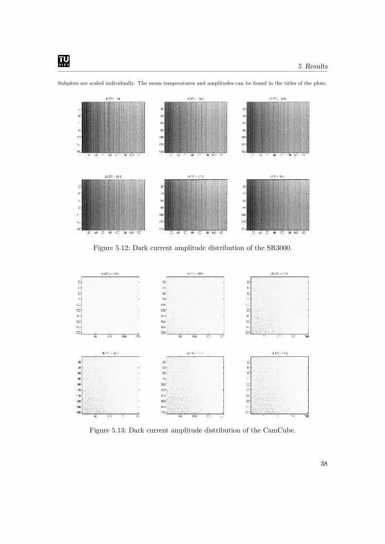
As expected, the cameras showed smaller signals at lower temperatures which is shown inFigures 5.12 and 5.13. The distribution of the amplitudes did not change along with thetemperature. This suggested that the sensor´s pixels can not be characterised the sameway. This might result from the production process which would make a chip-dependentcorrection necessary. A hint is given by the structure of the sensor as already depicted inFigure 2.3 on page 7.

The CamCube in contrast did not show such a regular increase over the chip area as theSR3000 did. It can be seen that the amplitudes increase in one corner and spread mostlyin the lower left corner. This might be related to different temperatures of the sensor orwithin the housing but could not be verified. Additionally an effect caused by the waythe pixels are read out was thought of.

37

5 Results

Subplots are scaled individually. The mean temperatures and amplitudes can be found in the titles of the plots.

Figure 5.12: Dark current amplitude distribution of the SR3000.

Figure 5.13: Dark current amplitude distribution of the CamCube.

38

5 Results

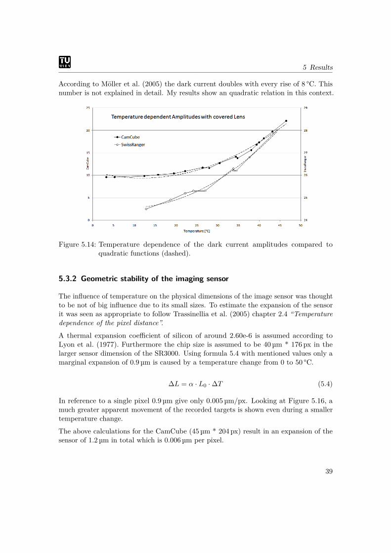
According to Möller et al. (2005) the dark current doubles with every rise of 8 °C. Thisnumber is not explained in detail. My results show an quadratic relation in this context.

Figure 5.14: Temperature dependence of the dark current amplitudes compared toquadratic functions (dashed).

5.3.2 Geometric stability of the imaging sensor

The influence of temperature on the physical dimensions of the image sensor was thoughtto be not of big influence due to its small sizes. To estimate the expansion of the sensorit was seen as appropriate to follow Trassinellia et al. (2005) chapter 2.4 “Temperaturedependence of the pixel distance”.

A thermal expansion coefficient of silicon of around 2.60e-6 is assumed according toLyon et al. (1977). Furthermore the chip size is assumed to be 40µm * 176 px in thelarger sensor dimension of the SR3000. Using formula 5.4 with mentioned values only amarginal expansion of 0.9 µm is caused by a temperature change from 0 to 50 °C.

∆L = α · L0 ·∆T (5.4)

In reference to a single pixel 0.9µm give only 0.005 µm/px. Looking at Figure 5.16, amuch greater apparent movement of the recorded targets is shown even during a smallertemperature change.The above calculations for the CamCube (45µm * 204 px) result in an expansion of thesensor of 1.2µm in total which is 0.006µm per pixel.

39

5 Results

Those small figures mean that the expansion of the sensor itself cannot be detectedseparately and is anyway negligible.

Nevertheless, the apparent movements of the targets are present as can clearly be seenin Figure 5.16 on the following page. This might be caused through a temperaturedependent mounting of the imaging sensor. Maybe the housing or other internal partsare not expanding equally.

If an thermal expansion coefficient for the aluminium housing of around 23.5e-43 isassumed, this means that one side of a camera with an original length of roughly 6 cm isthen increased by 70 µm. Considering the greater heating of the back of the CamCubeon one side (see. Fig. 5.1), this could result in a slight rotation of the sensor of about0.3mgon.

The analysis of movement of the calculated target centers was carried out as described inthe methods chapter on page 22. The repeatability is given in Figure 5.15. Also priorexperiments with the old mounting of the SR3000 showed the same movement pattern.

Figure 5.15: Repeatability of SR3000 Experiments. Two cooling down experiments.

3taken from the “Journal of Research of the National Bureau of Standards” Research Paper 2308, 1952

40

5 Results

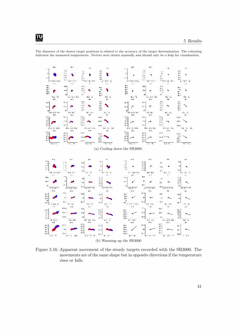
The diameter of the drawn target positions is related to the accuracy of the target determination. The colouringindicates the measured temperature. Vectors were drawn manually and should only be a help for visualisation.

(a) Cooling down the SR3000.

(b) Warming up the SR3000

Figure 5.16: Apparent movement of the steady targets recorded with the SR3000. Themovements are of the same shape but in opposite directions if the temperaturerises or falls.

41

5 Results

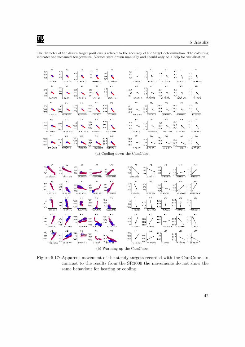
The diameter of the drawn target positions is related to the accuracy of the target determination. The colouringindicates the measured temperature. Vectors were drawn manually and should only be a help for visualisation.

(a) Cooling down the CamCube.

(b) Warming up the CamCube.

Figure 5.17: Apparent movement of the steady targets recorded with the CamCube. Incontrast to the results from the SR3000 the movements do not show thesame behaviour for heating or cooling.

42

5 Results

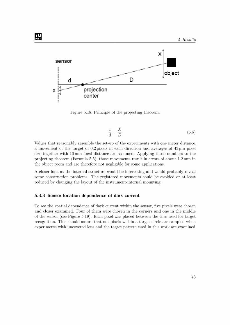
Figure 5.18: Principle of the projecting theorem.

x

d= X

D(5.5)

Values that reasonably resemble the set-up of the experiments with one meter distance,a movement of the target of 0.2 pixels in each direction and averages of 43µm pixelsize together with 10mm focal distance are assumed. Applying those numbers to theprojecting theorem (Formula 5.5), those movements result in errors of about 1.2mm inthe object room and are therefore not negligible for some applications.

A closer look at the internal structure would be interesting and would probably revealsome construction problems. The registered movements could be avoided or at leastreduced by changing the layout of the instrument-internal mounting.

5.3.3 Sensor-location dependence of dark current

To see the spatial dependence of dark current within the sensor, five pixels were chosenand closer examined. Four of them were chosen in the corners and one in the middleof the sensor (see Figure 5.19). Each pixel was placed between the tiles used for targetrecognition. This should assure that not pixels within a target circle are sampled whenexperiments with uncovered lens and the target pattern used in this work are examined.

43

5 Results

Figure 5.19: Placement of the sampling points. (black squares: CamCube, red circles: SR3000)

(a) Differences in the sensor of the SR3000. (b) Differences in the sensor of the CamCube.

Figure 5.20: Behaviour of dark current dependent on the location of the pixel of interest.

The results depicted in Figure 5.20 show certain trends. While the standard deviationcalculated with 10 values of the dark current amplitudes of the SR3000 could be wellfitted with a linear trend the CamCube´s data needed a quadratic function. Both camerashave larger deviations of amplitudes at higher temperatures as expected.

A closer look at the amplitude data of the SR3000 reveals that the slope of pixels in theleft part of the sensor are greater than the ones in the right part aside from pixel numbertwo.

The standard deviations derived from the CamCube show that pixels in the left partare most of the time larger than the other ones. This is consistent with the findings inchapter 5.3.1 on page 36. It must not be forgotten that the used housingtemperaturemight not be directly related to the temperature of the sensor.

44

5 Results

5.3.4 Influence on the active Illumination

It was expected that during operation the illumination would heat up until a certainpoint and also change its behaviour according to that elevated temperature. To tacklethis Rapp (2007) recommends more efficient light sources which seems to be an obvioussolution.

It is not known exactly which type of LEDs are used for the cameras but assuming similarproperties like for a GaAs-IR LED with a central wavelength of 950 nm a temperaturecoefficient of the radiation power of -0.55%/K is stated in Gluiber et al. (1993). Thismeans that an increasing temperature causes decreasing illumination power. For thetemperature range that is covered in this work (50 °C) this means a decrease of 27.5%.The amplitudes of the derived data do show such a correlation, which can be seen inFigure 5.7 for the SR3000 and in Figure 5.8 for the CamCube.

Furthermore, the temperature coefficient of the forward voltage coming to the LEDs isstated as major influence. Due to the fact that the cameras were not disassembled, thiscould not be further investigated.

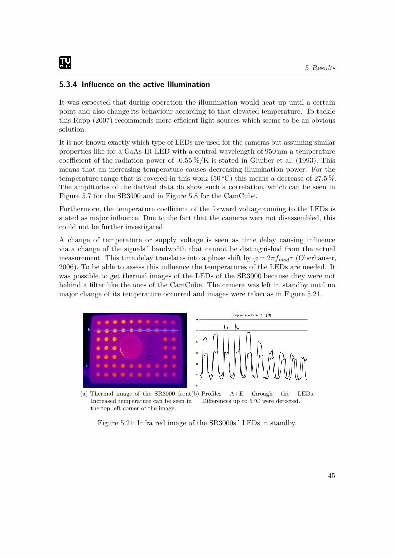
A change of temperature or supply voltage is seen as time delay causing influencevia a change of the signals´ bandwidth that cannot be distinguished from the actualmeasurement. This time delay translates into a phase shift by ϕ = 2πfmodτ (Oberhauser,2006). To be able to assess this influence the temperatures of the LEDs are needed. Itwas possible to get thermal images of the LEDs of the SR3000 because they were notbehind a filter like the ones of the CamCube. The camera was left in standby until nomajor change of its temperature occurred and images were taken as in Figure 5.21.

(a) Thermal image of the SR3000 front.Increased temperature can be seen inthe top left corner of the image.

(b) Profiles A+E through the LEDs.Differences up to 5 °C were detected.

Figure 5.21: Infra red image of the SR3000s´ LEDs in standby.

45

5 Results

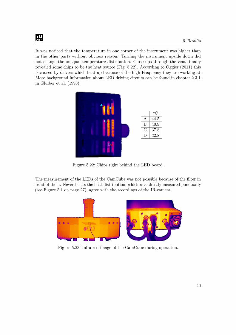
It was noticed that the temperature in one corner of the instrument was higher thanin the other parts without obvious reason. Turning the instrument upside down didnot change the unequal temperature distribution. Close-ups through the vents finallyrevealed some chips to be the heat source (Fig. 5.22). According to Oggier (2011) thisis caused by drivers which heat up because of the high Frequency they are working at.More background information about LED driving circuits can be found in chapter 2.3.1.in Gluiber et al. (1993).

°CA 44.5B 40.9C 37.8D 32.8

Figure 5.22: Chips right behind the LED board.

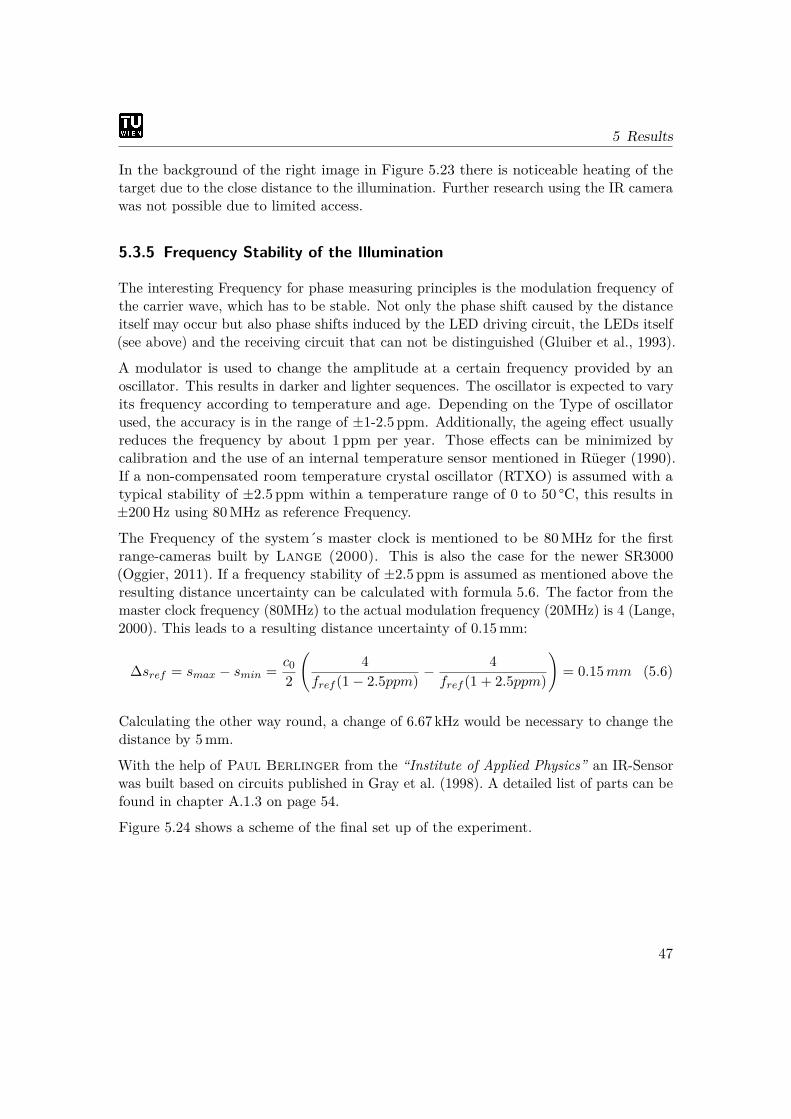
The measurement of the LEDs of the CamCube was not possible because of the filter infront of them. Nevertheless the heat distribution, which was already measured punctually(see Figure 5.1 on page 27), agree with the recordings of the IR-camera.

Figure 5.23: Infra red image of the CamCube during operation.

46

5 Results

In the background of the right image in Figure 5.23 there is noticeable heating of thetarget due to the close distance to the illumination. Further research using the IR camerawas not possible due to limited access.

5.3.5 Frequency Stability of the Illumination

The interesting Frequency for phase measuring principles is the modulation frequency ofthe carrier wave, which has to be stable. Not only the phase shift caused by the distanceitself may occur but also phase shifts induced by the LED driving circuit, the LEDs itself(see above) and the receiving circuit that can not be distinguished (Gluiber et al., 1993).

A modulator is used to change the amplitude at a certain frequency provided by anoscillator. This results in darker and lighter sequences. The oscillator is expected to varyits frequency according to temperature and age. Depending on the Type of oscillatorused, the accuracy is in the range of ±1-2.5 ppm. Additionally, the ageing effect usuallyreduces the frequency by about 1 ppm per year. Those effects can be minimized bycalibration and the use of an internal temperature sensor mentioned in Rüeger (1990).If a non-compensated room temperature crystal oscillator (RTXO) is assumed with atypical stability of ±2.5 ppm within a temperature range of 0 to 50 °C, this results in±200Hz using 80MHz as reference Frequency.

The Frequency of the system´s master clock is mentioned to be 80MHz for the firstrange-cameras built by Lange (2000). This is also the case for the newer SR3000(Oggier, 2011). If a frequency stability of ±2.5 ppm is assumed as mentioned above theresulting distance uncertainty can be calculated with formula 5.6. The factor from themaster clock frequency (80MHz) to the actual modulation frequency (20MHz) is 4 (Lange,2000). This leads to a resulting distance uncertainty of 0.15mm:

∆sref = smax − smin = c02

(4

fref (1− 2.5ppm) −4

fref (1 + 2.5ppm)

)= 0.15mm (5.6)

Calculating the other way round, a change of 6.67 kHz would be necessary to change thedistance by 5mm.

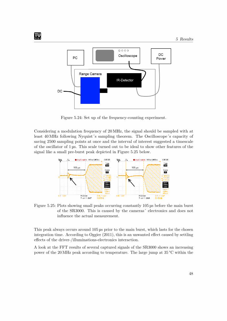
With the help of Paul Berlinger from the “Institute of Applied Physics” an IR-Sensorwas built based on circuits published in Gray et al. (1998). A detailed list of parts can befound in chapter A.1.3 on page 54.

Figure 5.24 shows a scheme of the final set up of the experiment.

47

5 Results

Figure 5.24: Set up of the frequency-counting experiment.

Considering a modulation frequency of 20MHz, the signal should be sampled with atleast 40MHz following Nyquist´s sampling theorem. The Oscilloscope´s capacity ofsaving 2500 sampling points at once and the interval of interest suggested a timescaleof the oscillator of 1 µs. This scale turned out to be ideal to show other features of thesignal like a small pre-burst peak depicted in Figure 5.25 below.

Figure 5.25: Plots showing small peaks occurring constantly 105µs before the main burstof the SR3000. This is caused by the cameras´ electronics and does notinfluence the actual measurement.

This peak always occurs around 105 µs prior to the main burst, which lasts for the chosenintegration time. According to Oggier (2011), this is an unwanted effect caused by settlingeffects of the driver-/illuminations-electronics interaction.

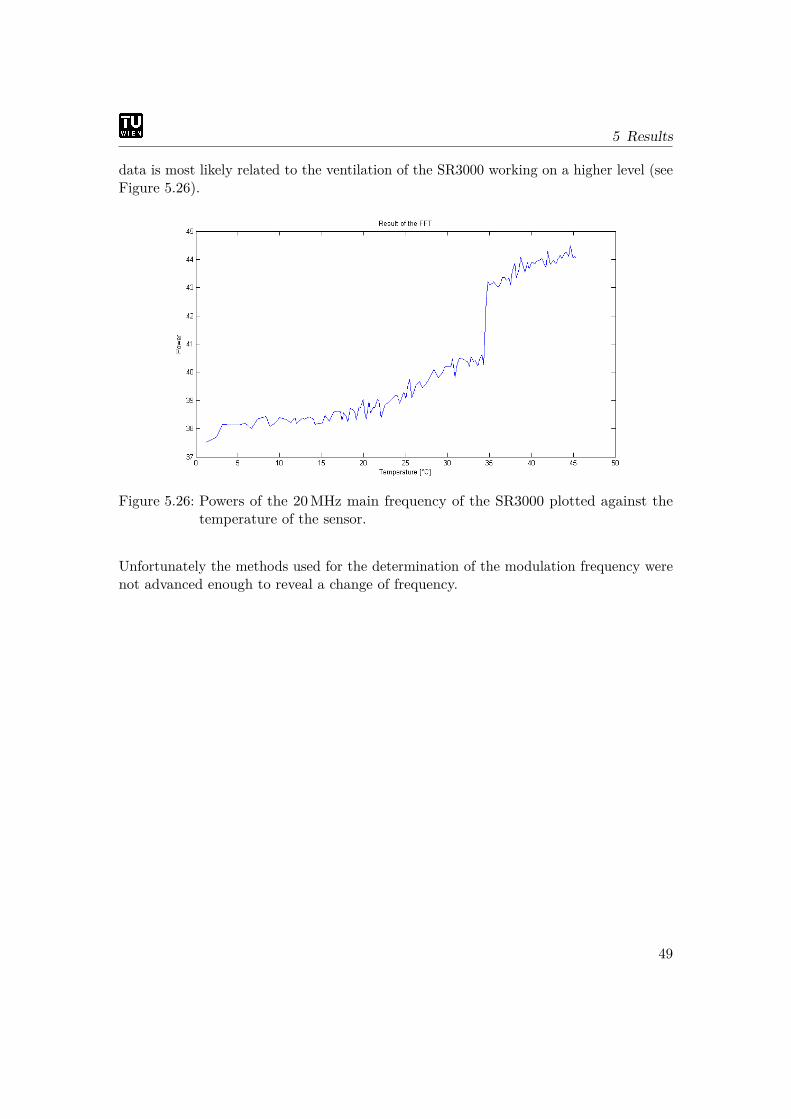
A look at the FFT results of several captured signals of the SR3000 shows an increasingpower of the 20MHz peak according to temperature. The large jump at 35 °C within the

48

5 Results

data is most likely related to the ventilation of the SR3000 working on a higher level (seeFigure 5.26).

Figure 5.26: Powers of the 20MHz main frequency of the SR3000 plotted against thetemperature of the sensor.

Unfortunately the methods used for the determination of the modulation frequency werenot advanced enough to reveal a change of frequency.

49

5 Results

5.4 Summary of Results

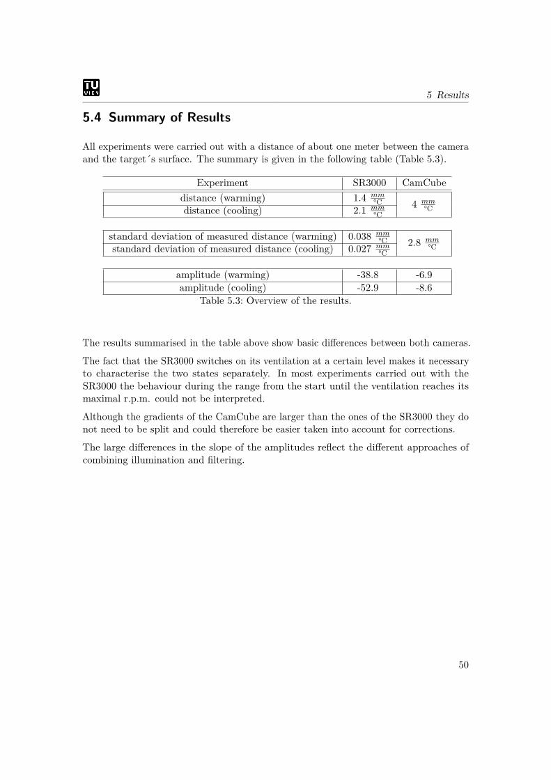
All experiments were carried out with a distance of about one meter between the cameraand the target´s surface. The summary is given in the following table (Table 5.3).

Experiment SR3000 CamCubedistance (warming) 1.4 mm

°C 4 mm°Cdistance (cooling) 2.1 mm

°C

standard deviation of measured distance (warming) 0.038 mm°C 2.8 mm

°Cstandard deviation of measured distance (cooling) 0.027 mm°C

amplitude (warming) -38.8 -6.9amplitude (cooling) -52.9 -8.6

Table 5.3: Overview of the results.

The results summarised in the table above show basic differences between both cameras.

The fact that the SR3000 switches on its ventilation at a certain level makes it necessaryto characterise the two states separately. In most experiments carried out with theSR3000 the behaviour during the range from the start until the ventilation reaches itsmaximal r.p.m. could not be interpreted.

Although the gradients of the CamCube are larger than the ones of the SR3000 they donot need to be split and could therefore be easier taken into account for corrections.

The large differences in the slope of the amplitudes reflect the different approaches ofcombining illumination and filtering.

50

6 Conclusion

6.1 Conclusions

It was found that temperature was influencing several different parts of range cameras. Amore detailed research on each of the topics visited in this work could be done to furtherdeepen the understanding of all temperature related effects.

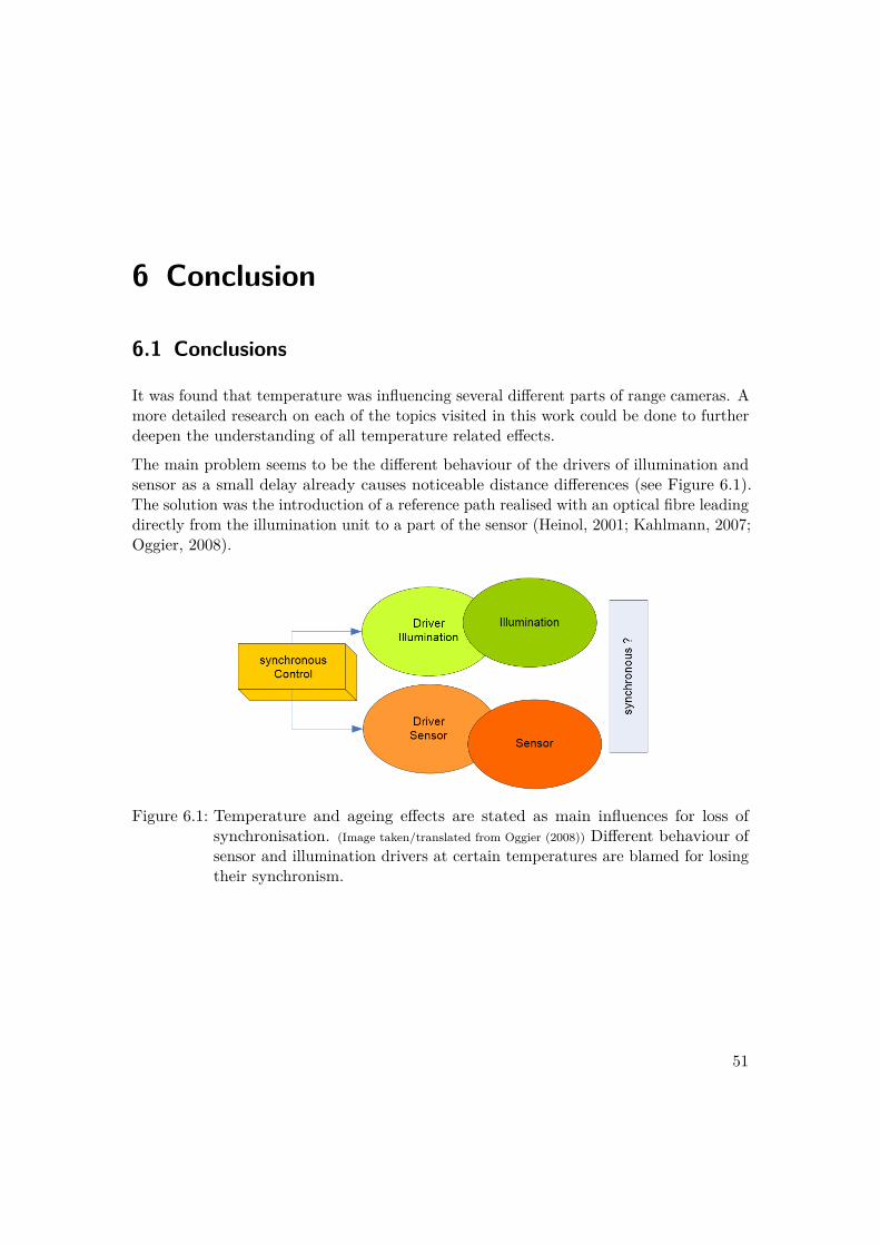
The main problem seems to be the different behaviour of the drivers of illumination andsensor as a small delay already causes noticeable distance differences (see Figure 6.1).The solution was the introduction of a reference path realised with an optical fibre leadingdirectly from the illumination unit to a part of the sensor (Heinol, 2001; Kahlmann, 2007;Oggier, 2008).

Figure 6.1: Temperature and ageing effects are stated as main influences for loss ofsynchronisation. (Image taken/translated from Oggier (2008)) Different behaviour ofsensor and illumination drivers at certain temperatures are blamed for losingtheir synchronism.

51

6 Conclusion

6.2 Temperature related recommendations for practical work

The use of the cameras at constant temperatures is an obvious way to avoid correcting thedata afterwards. This however is hardly realistic due to the fact that the temperaturesof the environment, the housing, the sensor, the illumination and the electronics have tobe at a steady state. Switching on and starting the measurement fairly in advance ofthe final observations turned out to be really helpful. This way switch-on effects did nothave to be considered.

A note in Rüeger (1990) states that the lifetime of GaAlAs diodes could be 10 timeslonger at 25 °C compared to operation at 50 °C. Also a drop of the emitting power to75% after 10 000 hours (more than a year) use at room temperature is mentioned. Thisimplies that continuous operation at elevated temperatures should be avoided to reduceunnecessary stress on material.

In respect to the oscillator, operation at a steady temperature is preferred, however notobligatory because temperature does not have a great impact on it (see Chapter 5.3.5).

Finally it should be thought of the possibility of condensation water when working atquickly changing environments.

6.3 Future Work

Previous works that use the integration time as base e.g. for their correction algorithmsmight be revisited to check if the use of temperature data related on that integrationtime might be more appropriate.

More detailed Experiments with the use of an appropriate climate chamber should becarried out. Thereby not only measurements at certain temperature levels should betaken but rather during changing temperatures to be able to differentiate between heatingand cooling effects. As final result a hysteresis of the heating and cooling effects on themeasurements is expected.

52

A Appendix

A.1 Instruments used for Experiments

Apart from the cameras and the PC for recording following instruments were used:

• Heating and cooling devices

• Data-Logger for recording the meteorology of the measurement laboratory

• Temperature-Logger for monitoring the temperatures of both cameras

A.1.1 Devices for heating and cooling

For reasons of convenience and because of the unavailability of a proper climatic chamber,everyday life devices present at the Institutes were used. Prior to the experiments it wasmade sure that they could reach all temperatures needed by a series of tests.

Oven

The oven used for heating up the cameras is a simple miniature baking oven. To avoidirregular warming by radiant heat, two shieldings of black cardboard with the sidepointing away of the heaters covered with aluminium foil were built in to ensure a muchsmoother rise and smaller variations of the temperature. The temperature differencesinside the oven were found to be around 2 °C and therefore in an acceptable range. Forreasons of security in respect to the cameras the maximum temperature was set severaldegrees below the highest allowed storing temperature.

Refrigerator

The ice box of a refrigerator was used to cool down the cameras below 0 °C. The cameraswere protected against direct cold airflows by a cardboard wall. Furthermore a thermalinsulation was introduced between the carton and the frigistors.

53

A Appendix

A.1.2 Temperature Loggers

Meteorology-Data-Logger

The ambient room temperature was monitored with a PCE-THB 401 thermohygrometerand barometer. Temperature humidity and pressure were recorded every five minutes.Recordings starting at the end of December 2010 show only small variations of thetemperature. More details can be found in Chapter 3.4.

Temperature Logger

For the recording of present temperatures a 4-channel Thermo-Data-Logger was used,which was in this case the PCE-T 390 with a temperature range of -100 °C up to morethan 1000 °C. The accuracy of 0.1 °C ± (0.4% + 0.5 °C)2 and a time resolution of upto a second were seen to be suitable for the measurements. Also the reaction time ofaround a second should not pose a problem.Nevertheless, it turned out to be necessary to check the recorded data for erroneoustemperature as well as equal timestamps following each other and hindering the automatedanalysis. While the erroneous temperature values were interpolated, the problem withthe timestamps was tackled within the analysis routine by keeping only the first uniquetimestamp.

Temperature Sensors

Two K-Type wire sensors that were delivered with the Temperature-Logger were usedto tune the oven and the cooling unit to the desired temperatures. An additional K-Type magnetic surface probe (thermo-electra3 Model: 80513) was used to determine thetemperature of the cameras. For the determination of the surface temperature of theCamCube (see Fig. 5.1) a thermo-electra surface probe (80102A) was used.

A.1.3 Instruments for Illumination Analysis

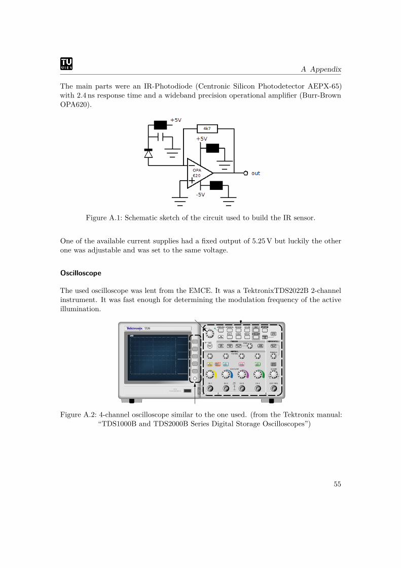
IR-Detector

To be able to detect the Modulation frequency of the illuminations, a sensitive receiverwas necessary. A circuit similar to the ones described in Gray et al. (1998) was developedand constructed by Paul Berlinger.1http://www.industrial-needs.com/measuring-instruments/thermo-hygrometers.htm2precision tested by the manufacturer at 23±5 °C (PCE Instruments, 2010)3http://www.thermo-electra.com/

54

http://www.industrial-needs.com/measuring-instruments/thermo-hygrometers.htm

http://www.thermo-electra.com/

A Appendix

The main parts were an IR-Photodiode (Centronic Silicon Photodetector AEPX-65)with 2.4 ns response time and a wideband precision operational amplifier (Burr-BrownOPA620).

Figure A.1: Schematic sketch of the circuit used to build the IR sensor.

One of the available current supplies had a fixed output of 5.25V but luckily the otherone was adjustable and was set to the same voltage.

Oscilloscope

The used oscilloscope was lent from the EMCE. It was a TektronixTDS2022B 2-channelinstrument. It was fast enough for determining the modulation frequency of the activeillumination.

Figure A.2: 4-channel oscilloscope similar to the one used. (from the Tektronix manual:“TDS1000B and TDS2000B Series Digital Storage Oscilloscopes”)

55

A Appendix

56

Bibliography

Besl, Paul J. (June 1988). “Active, optical range imaging sensors”. In: Machine Visionand Applications 1.2, pp. 127–152. issn: 0932-8092. doi: 10.1007/BF01212277. url:http://www.springerlink.com/index/10.1007/BF01212277.

Bureau International des Poids et Mesures (2006). Le Système international d’unités. 8th.1. Paris: STEDI MEDIA. isbn: 92-822-2213-6. url: http://www.bipm.org/utils/common/pdf/si_brochure_8_en.pdf.

Frey, Jochen (2008). Bildsensorik mit Tiefgang - Stand der PMD-Technik, Roadmap undPerspektiven. Tech. rep. Siegen: PMD Technologies GmbH. url: http://spectronet.de/portals/visqua/story_docs/vortraege_2008/081118_pmd_visionday/081118_01_frey_pmd_technologies.pdf.

Gluiber, W. et al. (1993). Optische Abstandsmessung. Haus der Technik - Fachbuchreihe.Essen: R. Pepperl.

Gray, Malcolm B. et al. (1998). “Photodetector designs for experiments in quantumoptics”. In: Rev. Sci. Instrum. Pp. 1–10. url: http://www.atom.fysik.lth.se/QI/laser_documentation/Selected_articles/PhotodetectordesignsforExperimentsinQuantumOptics.pdf.

Heinol, Horst G. (2001). “Untersuchung und Entwicklung von modulationslaufzeitbasierten3D-Sichtsystemen”. PhD thesis. University of Siegen. url: http://www.zess.uni-siegen.de/cms/diss/2001/heinol/heinol.pdf.

Kahlmann, Timo (2007). “Range imaging metrology: Investigation, calibration anddevelopment”. PhD thesis. ETH Zurich. doi: 10.3929/ethz-a-005465562. url:http://e-collection.ethbib.ethz.ch/view/eth:41869.

Kahlmann, Timo, Fabio Remondino, and Hilmar Ingensand (2006). “Calibration forIncreased Accuracy of the Range Imaging Camera Swissranger”. In: Proc. of IEVMXXXVI.4, pp. 136–141. url: http://citeseerx.ist.psu.edu/viewdoc/download?doi=10.1.1.62.8904&rep=rep1&type=pdf.

Karel, Wilfried (2007). “Range Imaging: 3D-Punktwolken in Echtzeit”. In: ÖsterreichischeZeitschrift für Vermessung und Geoinformation 4, pp. 1–12.

Karel, Wilfried, Sajid Ghuffar, and Norbert Pfeifer (2010). “Quantifying the Distortionof Distance Observations Caused by Scattering in Time-of-Flight Range Cameras”.

57

http://dx.doi.org/10.1007/BF01212277

http://www.springerlink.com/index/10.1007/BF01212277

http://www.bipm.org/utils/common/pdf/si_brochure_8_en.pdf

http://www.bipm.org/utils/common/pdf/si_brochure_8_en.pdf

http://spectronet.de/portals/visqua/story_docs/vortraege_2008/081118_pmd_visionday/081118_01_frey_pmd_technologies.pdf



http://www.atom.fysik.lth.se/QI/laser_documentation/Selected_articles/Photodetector designs for Experiments in Quantum Optics.pdf



http://www.zess.uni-siegen.de/cms/diss/2001/heinol/heinol.pdf

http://www.zess.uni-siegen.de/cms/diss/2001/heinol/heinol.pdf

http://dx.doi.org/10.3929/ethz-a-005465562

http://e-collection.ethbib.ethz.ch/view/eth:41869

http://citeseerx.ist.psu.edu/viewdoc/download?doi=10.1.1.62.8904&rep=rep1&type=pdf


Bibliography

In: ISPRS XXXVIII. url: http://www.isprs.org/proceedings/XXXVIII/part5/papers/228.pdf.

Lange, Robert (2000). “3D time-of-flight distance measurement with custom solid-stateimage sensors in CMOS/CCD-technology”. PhD thesis. University of Siegen. url:http://dokumentix.ub.uni-siegen.de/opus/volltexte/2006/178/.

Lange, Robert and Peter Seitz (Mar. 2001). “Solid-state time-of-flight range camera”.In: IEEE Journal of Quantum Electronics 37.3, pp. 390–397. issn: 00189197. doi:10.1109/3.910448. url: http://ieeexplore.ieee.org/lpdocs/epic03/wrapper.htm?arnumber=910448.

Luan, Xuming (2001). “Experimental Investigation of Photonic Mixer Device andDevelopment of TOF 3D Ranging Systems Based on PMD Technology”. PhDthesis. University of Siegen. url: http://www.zess.uni-siegen.de/cms/diss/2001/luan/luan.pdf.

Lyon, K. G. et al. (1977). “Linear thermal expansion measurements on silicon from 6to 340 K”. In: Journal of Applied Physics 48.3, pp. 865–868. issn: 0021-8979. url:http://ieeexplore.ieee.org/xpls/abs_all.jsp?arnumber=5103488.

Mesa Imaging (2006). SwissRanger SR-3000 Manual. Zürich. url: http://aiweb.techfak.uni-bielefeld.de/files/SR3000_manual_V1.03.pdf.

— (2008). SR-3000 Data Sheet. Zürich. url: http://www.mesa-imaging.ch/pdf/SR3000_Flyer_Jan07.pdf.

Möller, Tobias et al. (2005). Robust 3D Measurement with PMD Sensors. Tech. rep.Zürich. url: http://citeseerx.ist.psu.edu/viewdoc/download?doi=10.1.1.132.5821&rep=rep1&type=pdf.

Oberhauser, Klaus (2006). “Opto-Electronic Integrated Correlation Receivers for Time-of-Flight Based Distance Measurement Systems”. Dissertation. Vienna University ofTechnology. url: http://www.ub.tuwien.ac.at/diss/AC05033224.pdf.

Oggier, Thierry (2008). 3D-Bilderfassung in Echtzeit mit modernen hochintegrierten3D-Kameras. Stuttgart.

— (Aug. 2011). personal communication.Oggier, Thierry et al. (2005). “Swissranger SR3000 and First Experiences based on

Miniaturized 3D-TOF Cameras”. In: Proceedings of the First Range Imaging ResearchDay at ETH Zurich. url: http://j-clavis.co.jp/pdf/h-4.pdf.

Otepka, Johannes (2004). “Precision Target Mensuration in Vision Metrology”. PhD thesis.Vienna University of Technology. url: http://media.obvsg.at/AC04346920-2001.

Pattinson, Timothy (2010). “Quantification and Description of Distance MeasurementErrors of a Time-of-Flight Camera”. MA thesis. University of Stuttgart. url: http:

58

http://www.isprs.org/proceedings/XXXVIII/part5/papers/228.pdf

http://www.isprs.org/proceedings/XXXVIII/part5/papers/228.pdf

http://dokumentix.ub.uni-siegen.de/opus/volltexte/2006/178/

http://dx.doi.org/10.1109/3.910448

http://ieeexplore.ieee.org/lpdocs/epic03/wrapper.htm?arnumber=910448

http://ieeexplore.ieee.org/lpdocs/epic03/wrapper.htm?arnumber=910448

http://www.zess.uni-siegen.de/cms/diss/2001/luan/luan.pdf

http://www.zess.uni-siegen.de/cms/diss/2001/luan/luan.pdf

http://ieeexplore.ieee.org/xpls/abs_all.jsp?arnumber=5103488

http://aiweb.techfak.uni-bielefeld.de/files/SR3000_manual_V1.03.pdf

http://aiweb.techfak.uni-bielefeld.de/files/SR3000_manual_V1.03.pdf

http://www.mesa-imaging.ch/pdf/SR3000_Flyer_Jan07.pdf

http://www.mesa-imaging.ch/pdf/SR3000_Flyer_Jan07.pdf



http://www.ub.tuwien.ac.at/diss/AC05033224.pdf

http://j-clavis.co.jp/pdf/h-4.pdf

http://media.obvsg.at/AC04346920-2001

http://www.lulu.com/items/volume_68/8652000/8652310/1/print/distance_errors_tof_camera-1.pdf


Bibliography

//www.lulu.com/items/volume_68/8652000/8652310/1/print/distance_errors_tof_camera-1.pdf.

PCE Instruments (2010). Manual: Digital Thermometer PCE-T 390. Durham. url:http://www.industrial-needs.com/manual/manual-pce-t390.pdf.

PMD Technologies (2009). Datasheet: PMD[vision] CamCube 2.0. Siegen. url: http://www.pmdtec.com/fileadmin/pmdtec/downloads/documentation/datasheet_camcube.pdf.

Rapp, Holger (2007). “Experimental and Theoretical Investigation of Correlating TOF-Camera Systems”. PhD thesis. University of Heidelberg. url: http://www.ub.uni-heidelberg.de/archiv/7666/.

Ringbeck, Thorsten and Bianca Hagebeuker (2007). “Dreidimensionale Objekterfassung inEchtzeit - PMDKameras erfassen pro Pixel Distanz und Helligkeit mit Videoframerate”.In: AVN, pp. 263–270.

Rüeger, Jean M. (1990). Electronic Distance Measurement: An Introduction. 3rd. Berlin;Heidelberg: Springer, p. 266.

Schneider, Bernd (2003). “Der Photomischdetektor zur schnellen 3D-Vermessung fürSicherheitssysteme und zur Informationsübertragung im Automobil”. PhD thesis.University of Siegen. url: http://dokumentix.ub.uni-siegen.de/opus/volltexte/2005/43/.

Steiger, Oliver, Judith Felder, and Stephan Weiss (2008). “Calibration of time-of-flight range imaging cameras”. In: Image Processing, 2008. ICIP 2008. 15th IEEEInternational Conference on. IEEE, pp. 1968–1971. url: http://ieeexplore.ieee.org/xpls/abs_all.jsp?arnumber=4712168.

Trassinellia, M. et al. (2005). “Characterization of the geometry of an array of CCD pixeldetectors”. In: International Conference on Exotic Atoms and Related Topics. Vienna,pp. 343–348. url: http://www.austriaca.at/0xc1aa500d_0x000fd4f7.pdf.

Weyer, Christoph A. et al. (2008). “Extensive metric performance evaluation of a 3D rangecamera”. In: ISPRS 37.1, pp. 939–944. url: http://www.isprs.org/proceedings/XXXVII/congress/5_pdf/163.pdf.

Zach, Gerald, Milos Davidovic, and Horst Zimmermann (2010). “A 16 times 16 PixelDistance Sensor With In-Pixel Circuitry That Tolerates 150 klx of Ambient Light”.In: Solid-State Circuits, IEEE Journal of 45.7, pp. 1345–1353. url: http://ieeexplore.ieee.org/xpls/abs_all.jsp?arnumber=5492315.

59




http://www.industrial-needs.com/manual/manual-pce-t390.pdf

http://www.pmdtec.com/fileadmin/pmdtec/downloads/documentation/datasheet_camcube.pdf



http://www.ub.uni-heidelberg.de/archiv/7666/

http://www.ub.uni-heidelberg.de/archiv/7666/





http://www.austriaca.at/0xc1aa500d_0x000fd4f7.pdf

http://www.isprs.org/proceedings/XXXVII/congress/5_pdf/163.pdf

http://www.isprs.org/proceedings/XXXVII/congress/5_pdf/163.pdf



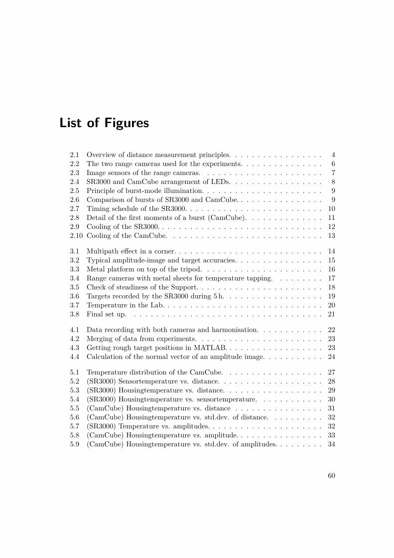
List of Figures

2.1 Overview of distance measurement principles. . . . . . . . . . . . . . . . . 42.2 The two range cameras used for the experiments. . . . . . . . . . . . . . . 62.3 Image sensors of the range cameras. . . . . . . . . . . . . . . . . . . . . . 72.4 SR3000 and CamCube arrangement of LEDs. . . . . . . . . . . . . . . . . 82.5 Principle of burst-mode illumination. . . . . . . . . . . . . . . . . . . . . . 92.6 Comparison of bursts of SR3000 and CamCube. . . . . . . . . . . . . . . . 92.7 Timing schedule of the SR3000. . . . . . . . . . . . . . . . . . . . . . . . . 102.8 Detail of the first moments of a burst (CamCube). . . . . . . . . . . . . . 112.9 Cooling of the SR3000. . . . . . . . . . . . . . . . . . . . . . . . . . . . . . 122.10 Cooling of the CamCube. . . . . . . . . . . . . . . . . . . . . . . . . . . . 13

3.1 Multipath effect in a corner. . . . . . . . . . . . . . . . . . . . . . . . . . . 143.2 Typical amplitude-image and target accuracies. . . . . . . . . . . . . . . . 153.3 Metal platform on top of the tripod. . . . . . . . . . . . . . . . . . . . . . 163.4 Range cameras with metal sheets for temperature tapping. . . . . . . . . 173.5 Check of steadiness of the Support. . . . . . . . . . . . . . . . . . . . . . . 183.6 Targets recorded by the SR3000 during 5 h. . . . . . . . . . . . . . . . . . 193.7 Temperature in the Lab. . . . . . . . . . . . . . . . . . . . . . . . . . . . . 203.8 Final set up. . . . . . . . . . . . . . . . . . . . . . . . . . . . . . . . . . . 21

4.1 Data recording with both cameras and harmonisation. . . . . . . . . . . . 224.2 Merging of data from experiments. . . . . . . . . . . . . . . . . . . . . . . 234.3 Getting rough target positions in MATLAB. . . . . . . . . . . . . . . . . . 234.4 Calculation of the normal vector of an amplitude image. . . . . . . . . . . 24

5.1 Temperature distribution of the CamCube. . . . . . . . . . . . . . . . . . 275.2 (SR3000) Sensortemperature vs. distance. . . . . . . . . . . . . . . . . . . 285.3 (SR3000) Housingtemperature vs. distance. . . . . . . . . . . . . . . . . . 295.4 (SR3000) Housingtemperature vs. sensortemperature. . . . . . . . . . . . 305.5 (CamCube) Housingtemperature vs. distance . . . . . . . . . . . . . . . . 315.6 (CamCube) Housingtemperature vs. std.dev. of distance. . . . . . . . . . 325.7 (SR3000) Temperature vs. amplitudes. . . . . . . . . . . . . . . . . . . . . 325.8 (CamCube) Housingtemperature vs. amplitude. . . . . . . . . . . . . . . . 335.9 (CamCube) Housingtemperature vs. std.dev. of amplitudes. . . . . . . . . 34

60

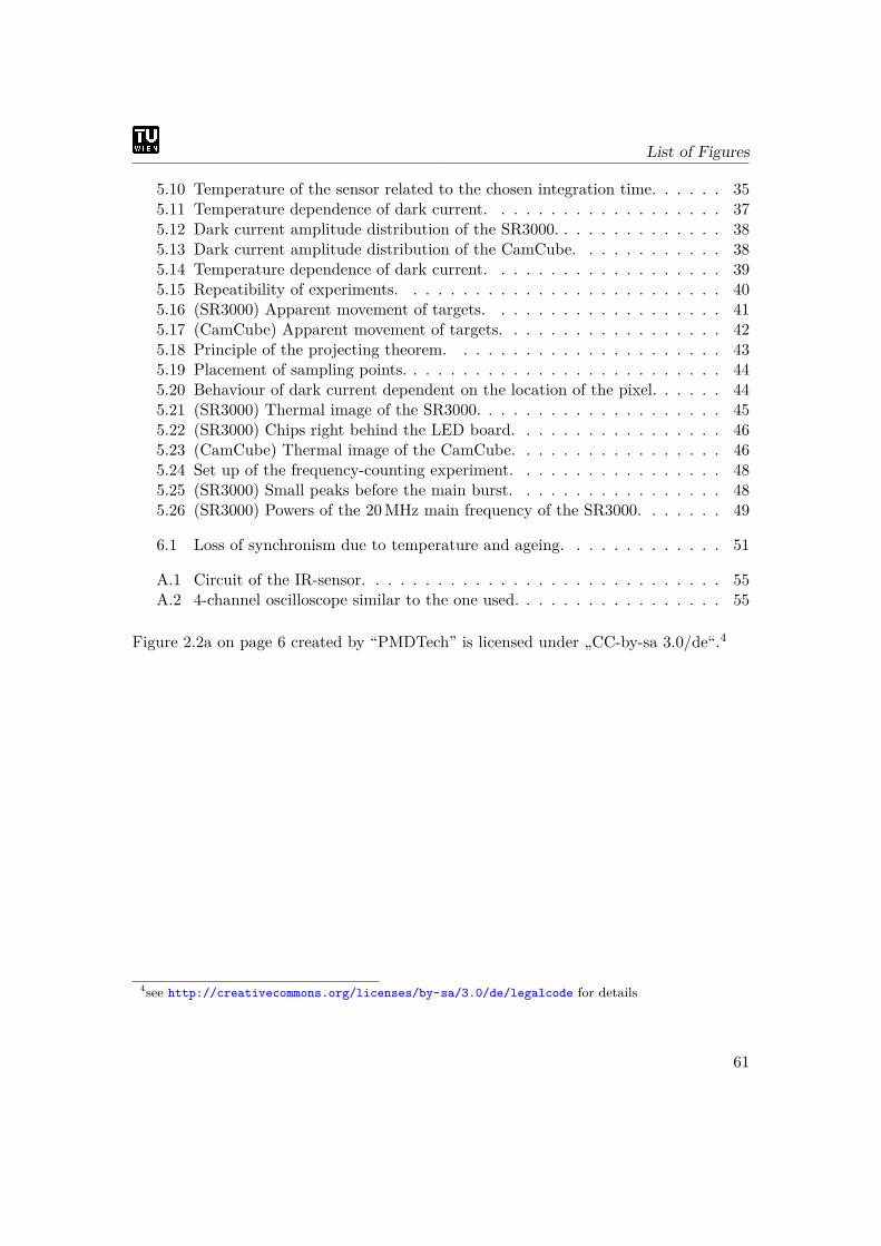
List of Figures

5.10 Temperature of the sensor related to the chosen integration time. . . . . . 355.11 Temperature dependence of dark current. . . . . . . . . . . . . . . . . . . 375.12 Dark current amplitude distribution of the SR3000. . . . . . . . . . . . . . 385.13 Dark current amplitude distribution of the CamCube. . . . . . . . . . . . 385.14 Temperature dependence of dark current. . . . . . . . . . . . . . . . . . . 395.15 Repeatibility of experiments. . . . . . . . . . . . . . . . . . . . . . . . . . 405.16 (SR3000) Apparent movement of targets. . . . . . . . . . . . . . . . . . . 415.17 (CamCube) Apparent movement of targets. . . . . . . . . . . . . . . . . . 425.18 Principle of the projecting theorem. . . . . . . . . . . . . . . . . . . . . . 435.19 Placement of sampling points. . . . . . . . . . . . . . . . . . . . . . . . . . 445.20 Behaviour of dark current dependent on the location of the pixel. . . . . . 445.21 (SR3000) Thermal image of the SR3000. . . . . . . . . . . . . . . . . . . . 455.22 (SR3000) Chips right behind the LED board. . . . . . . . . . . . . . . . . 465.23 (CamCube) Thermal image of the CamCube. . . . . . . . . . . . . . . . . 465.24 Set up of the frequency-counting experiment. . . . . . . . . . . . . . . . . 485.25 (SR3000) Small peaks before the main burst. . . . . . . . . . . . . . . . . 485.26 (SR3000) Powers of the 20MHz main frequency of the SR3000. . . . . . . 49

6.1 Loss of synchronism due to temperature and ageing. . . . . . . . . . . . . 51

A.1 Circuit of the IR-sensor. . . . . . . . . . . . . . . . . . . . . . . . . . . . . 55A.2 4-channel oscilloscope similar to the one used. . . . . . . . . . . . . . . . . 55

Figure 2.2a on page 6 created by “PMDTech” is licensed under „CC-by-sa 3.0/de“.4

4see http://creativecommons.org/licenses/by-sa/3.0/de/legalcode for details

61

http://creativecommons.org/licenses/by-sa/3.0/de/legalcode

List of Tables

2.1 Storage- and operating-temperatures. . . . . . . . . . . . . . . . . . . . . . 132.2 Focal lengths and modulation frequencies of the cameras. . . . . . . . . . 13

5.1 Temperatures of the CamCube in standby. . . . . . . . . . . . . . . . . . . 265.2 Safety limits ts for a two-tailed statistical security S of 95% depending on

the redundancy k. . . . . . . . . . . . . . . . . . . . . . . . . . . . . . . . 345.3 Overview of the results. . . . . . . . . . . . . . . . . . . . . . . . . . . . . 50

62

Curriculum Vitae

Philipp Zachhuber, born 25.08.1984 in Wels, AustriaVolunteering paramedic since 2004. Ambulance driver since 2005. Permission for working full-time as paramedic since 2006.

Education:2009-2011 Master “Survey and Land Registration”

2008-2009 ERASMUS Year Abroad: “University College London” (UCL)

2005-2008 Bachelor “Geodesy and Geomatics Engineering”5

1999-2004 Federal Higher Technical Institute for Civil Engineering “HTL 1 Linz”

1995-1999 Grammar school “BRG-Steyr”

1991-1995 Primary school Bad Hall

Work Experience: Numbers in brackets = working weeks

1. (4) Swietelsky Bauges.m.b.H

2. (8) Vermessungsbüro Dipl.-Ing. Walter Höllhuber

3. (4) Alpine Mayreder Bau GmbH

4. (9) OÖ Boden- und Baustoffprüfstelle GmbH

5. (5) OÖ Boden- und Baustoffprüfstelle GmbH

6. (4) Vermessungskanzlei D.I. Rudolf Schöffmann


8. (6) Österreichische Bundesforste AG

9. (2) Österreichisches Rotes Kreuz, LV OÖ

10. (4) Österreichische Bundesforste AG

11. (8) Deutsches Zentrum für Luft- und Raumfahrt

12. (2) Österreichisches Rotes Kreuz, LV OÖ


14. (12) Leica Geosystems5Thesis: “Investigation of correlations between coordinates from the ‚Austrian Federal Forests’ and theland surveying office”

63

impact of temperature and temperature-change on … · impact of temperature and temperature-change...

Documents