Impact of Mild-Hybrid Functionality on Fuel Economy and Battery Lifetime

M.F.A. Lammers Report number: DCT-2006-41

May 2006

TU/e Master Thesis Report May 2006 Supervisors: Prof.dr.ir. M. Steinbuch dr. P.A. Veenhuizen ir. M.W.T. Koot Technical University of Eindhoven dr.ir. N.P.I. Aneke dipl.ing. S.H.M.G. Ploumen Ford Research Centre Aachen, Aachen, Germany Powertrain Research & Advanced Engineering Europe Energy Management Group

2

Abstract Because air pollution due to car exhaust gasses is increasingly becoming a problem in today's society, relatively short-term solutions as the hybrid vehicle are being investigated. The subject of this report was to investigate the possible fuel consumption reduction in a mild-hybrid vehicle of features as regenerative braking, power assist and stop-start. For this purpose, a control strategy for a belt driven ISG suitable for generating a relatively small electric power has been designed. This strategy is able to calculate the optimal way to charge and discharge the battery online, so when the drive-cycle is not known in advance. The first step in calculating the optimal fuel consumption benefit due to ISG-control for an online strategy was to calculate the maximum fuel consumption reduction possible in a situation where the cycle is known in advance. The method that has been used for this calculation is Dynamic Programming. The second step was to approach this benefit with an online strategy. Both a heuristic and an analytical strategy have been designed for this purpose. The first is a strategy, which chooses for generation or power assist, depending on certain vehicle's parameters such as the acceleration or propulsion power and torque outputs. The second strategy determines a generating and assisting efficiency and selects charging or discharging when it is beneficial to do so from an energetic point of view. Both strategies were tested in an acknowledged and validated computer model, called CVSP. In addition, the fuel saving due to stop-start and possibilities in order to maximize the fuel consumption reduction of the mild-hybrid features have been investigated. Simulations were done in an existing and acknowledged computer model designed by Ford.

3

Contents Abstract 2 1 Introduction 5 1.1 Hybrid Electric Vehicles 5 1.2 Goal of the project 7 1.3 Methodology 7 1.4 Thesis layout 8 2 Vehicle model 9 2.1 Simulink CVSP powertrain model 9 2.2 Test car specifications 10 2.3 Battery 12 2.4 ISG 14 3 Dynamic Programming 15 3.1 Method 15 3.2 Results 16 3.2.1 ISG with constant efficiency 16 3.2.2 ISG with variable efficiency 20 3.2.3 Grid size variation 23 3.2.4 Voltage model 24 3.3.5 Conclusions 26 4 Control Strategies 27 4.1 Heuristic control strategy 27 4.1.1 Strategy results 29 4.2 Analytical control strategy 34 4.2.1 Total system 34 4.2.2 The ICE 34 4.2.3 The ISG 36

4.2.4 The Battery 36 4.2.5 Charging 37 4.2.6 Discharging 38 4.2.7 Strategy results 38 4.2.8 Emissions 45 4.2.9 Dual battery system 46 4.2.10 Battery charge acceptance 51 4.2.11 D-ISG configuration 52 4.3 Stop-start 56 4.4 Battery lifetime 58 4.5 Conclusions 59 5 Conclusions and recommendations 60 5.2 Strategies and FC reductions of mild-hybrid features 60 5.1 Dynamic Programming 60 5.3 Dual voltage system and D-ISG 61 5.4 Battery lifetime 61 References 63 List of abbreviations 65

4

Symbols 66 Appendix A ICE efficiency map and NEDC cycle 68 Appendix B Optimal paths on NEDC cycle for 20 and 30 [A] electric loads 69 Appendix C Optimal trajectories for different grid sizes 70 Appendix D Used values for heuristic parameters 71 Appendix E Results of the heuristic strategy on EPA cycles 72 Appendix F Results of the analytical strategy on EPA cycles 73 Appendix G Influence of battery charge acceptance on fuel consumption 74

5

Chapter 1

Introduction The electrical power level and weight of the modern car are continuously rising due to numerous electrical systems, such as electric windows, power steering and climate control. Despite these increases, the customer expects a reduction in fuel economy and emission levels with each new car generation. Car manufacturers are searching for solutions in order to meet the fuel economy and emission demands, even with a higher average electrical load and vehicle weight. These solutions can be focused on the long run, for example fuel cell powered vehicles, or on the more nearby future. In the last category, hybrid vehicles are interesting possibilities. These vehicles can be equipped with features like stop-start, regenerative braking and power assist. 1.1. Hybrid Electric Vehicles A hybrid vehicle is equipped with two or more power sources. Generally these power-sources are a conventional combustion engine (usually diesel or petrol) and an electric motor. A distinction of hybrid vehicles into two main groups can be made: serial and parallel hybrids. In the serial hybrid, the primary power source (the combustion engine) is not mechanically linked to the powertrain, but it is used to supply power to a storage device. The secondary power source (the electric motor) can then draw its energy from this storage-device and propel the vehicle. In the parallel hybrid configuration, both power sources are mechanically linked to the wheels. The possibilities of the parallel hybrid vehicle will be explored further in this investigation. More information about hybrids in the literature can be found for instance in [1], [2] and [4]. There are 4 different classes in hybridization of the (parallel) hybrid vehicle; micro-, mild-, medium- and full-hybrids. The distinction is made in functionality, rated electrical power and voltage level, see Figure 1.1. This research will be focused on a hybrid vehicle with a small electrical power up to approximately 10 [kW]. With these small electric powers, a relatively high benefit can already be obtained, see [3] and [4]. The voltage level of a mild-hybrid is usually 36 [V], but with the smallest electrical powers, such a high voltage level may not be required and 12 [V] might be a better solution. Because of the ability of some power/launch assist and regenerative braking, the used vehicle configuration is categorised as a mild-hybrid.

6

Figure 1.1: Different classes of hybridization [4] A conventional powertrain consists of a starter and a generator/alternator. The starter can convert electrical energy into mechanical energy and is used to crank the engine. The generator is basically the opposite. It is linked to the crankshaft and operates as a dynamo, transforming the ICE's (Internal Combustion Engine) mechanical power into electrical power and storing this power in the car's battery. The ISG (integrated starter generator) is a device that combines both functions. In generating mode it is charging the battery and in starting (or motor) mode it is discharging the battery in order to assist or start the ICE. There are multiple possible positions for the ISG to be installed. The 3 main configurations are the belt driven ISG (B-ISG), the crankshaft-mounted ISG (C-ISG) and the drivetrain-mounted ISG (D-ISG), see Figures 1.2 trough 1.4. The C- and D-ISG are generally used for larger electrical power levels than the B-ISG. The reason for this is the limited power that can be transferred without slip via the belt of the B-ISG. In case of a D-ISG, the clutch is located between the ICE and ISG, so the vehicle can run on either the ISG or on the combination of both power sources. Logically, if the vehicle must be able to run completely on the ISG, the electrical power should be large enough.

Figure 1.2: Schematic representation of a B-ISG

7

Figure 1.3: Schematic representation of a C-ISG

Figure 1.4: Schematic representation of a D-ISG An advantage of the D-ISG with respect to the other variants is that during deceleration the drag torque of the combustion engine can be eliminated by opening the clutch, making more energy available for regenerative braking. However, due to the limited charge acceptance of the battery, the full potential of regenerative braking is never utilised unless deceleration is very slow. Furthermore, installing a B-ISG system is less expensive, which gives it an important advantage over the C- and D-ISG. Since the priority of the project lies with investigating the fuel consumption benefit of a vehicle with a B-ISG, simulations will be limited to B-ISG driven hybrids at first. Later on, the FC potential will be studied for the D-ISG concept as an alternative. 1.2. Goal of the project The goal of the project is to determine the possible fuel consumption benefit of mild-hybrid features, such as power assist, regenerative braking and stop-start. This will be done via the implementation of a smart control strategy for a B-ISG in a hybrid vehicle with a specified diesel engine. Similar research in the field of energy management optimalisation with an ISG has already been done before, for example in [5], [6], [7], [8], [9] and [10]. In this case the reduction with a B-ISG is studied of a relatively small electrical power, up to approximately 10 [kW] maximally. The strategy has to be online, so the drive cycle is not known beforehand, like in every day driving situations. Furthermore, the consequences of the mild-hybrid features on battery throughput and lifetime will be investigated. Finally, recommendations with respect to the electrical architecture and the battery system will be made. The research will be carried out in the Energy Management group from the Ford Research Centre (FFA) located in Aachen, Germany. 1.3. Methodology The first contributing factor to a fuel consumption benefit in a hybrid vehicle is regenerative braking. The principle of regenerative braking is simple; during deceleration of the vehicle, kinetic energy is converted into electric energy by the ISG and then stored in the car's battery. Whereas in a normal car configuration, without regenerative braking, the kinetic energy would be dissipated in heat by the mechanical brakes and thus lost, regenerative braking allows the vehicle to regain a part of this

8

energy to cover for instance the electric load of the car's equipment, such as electric windows, lights etc. Another way to use this energy is to allow the ISG to convert the electrical energy back into mechanical energy in order to help propel the vehicle. This phenomenon is called power assist. When power assist is applied during acceleration of the vehicle from standstill, it is usually referred to as launch assist. The maximal FC benefit that can be obtained with regenerative braking will depend on the electrical power that can be stored. This is mainly dependent on the maximal charge acceptance of the battery. Therefore, the relation between fuel consumption saving and battery charge acceptance will be investigated. The second idea to get a fuel consumption reduction is a smart charging and discharging strategy. It functions due to the variable relation between fuel rate and mechanical power in the engine map, which will be explained later. At constant engine speed, the relation between fuel rate and mechanical power is not proportional, meaning that there will be points in the engine map where it is beneficial to generate or deliver assist and places where it will be uneconomical. The baseline strategy always charges the powernet load and does not consider the cost of charging/discharging. A smart strategy will be designed and applied in combination with regenerative braking. Stop-start is the final feature that will be investigated. With stop-start, the ICE is automatically shut down during a vehicle standstill phase, when the gear is in neutral. When the clutch pedal is pressed in order to select a gear, the ICE is automatically started up again. At first, stop-start will not be included in the control strategies. After the benefit of regenerative braking and power assist is established, stop-start is included in the strategy. 1.4. Thesis layout Before the online control strategy can be developed, the maximal possible fuel saving will be determined in the case of a known cycle beforehand. This information will be obtained via Dynamic Programming, which will be further explained in Chapter 3. When this optimum is computed, it is investigated whether control strategies will be able to approach the optimal fuel consumption reduction with an online strategy. The heuristic and analytical strategy will be described in Chapter 4 (respectively paragraph 4.1 and 4.2). The verification of the potential fuel consumption saving will be accomplished by implementation of the strategies in a Matlab/Simulink ® model, called the Simulink CVSP powertrain model, developed by Ford Motor Company.

9

Chapter 2

Vehicle Model In this chapter, the vehicle simulation model used to validate the control strategies will be explained. The vehicle and engine used in the simulations are also introduced and key elements such as the battery and the ISG are discussed. 2.1. Simulink CVSP powertrain model The control strategies will be implemented in a vehicle simulation environment created in Matlab/Simulink called CVSP (Corporate Vehicle Simulation Program). Although CVSP originates from 1985, a Simulink version has not been created until 2001. The original version was Fortran-based. The advantage of CVSP is that the model database is centrally administered and the models have been validated and are up-to-date. This makes comparing different strategies objective, since the simulation environment is equal for all users. The model is divided into multiple systems that interact with each other. Data is collected about many variables and other variables can be added at will. The data of all observed variables as a function of time eventually ends up in a system called the 'data-bin'. It is attempted to keep a certain oversight, by using subsystems in each system. Each subsystem can in turn have one or more subsystems in it, causing the number of layers in some systems to be as high as 5 or 10. Despite the attempt to keep the model structured, the complexity of the CVSP model is high. However, this is unavoidable if a complex system as a car is modelled in detail. The upper mask is shown in Figure 2.1, which shows the main systems.

Figure 2.1: Upper mask of the CVSP model A simplified schematic overview of the workings of the (for this research) relevant part of the CVSP model is given in Figure 2.2. A PID-controller in the driver system calculates the position of the throttle and brake-pedal based on the difference between the reference speed (for instance the NEDC cycle) and the actual speed.

10

Figure 2.2: Relevant part of the control loop of the CVSP model The master controller (MSC) calculates the current that the ISG should deliver, denoted by I'ISG, and sends this signal to the ISG, located in the auxiliary system (AUX). This current is equal than drawn from the battery (BATT). Note that the battery current (IBATT) and the ISG current (IISG) are not equal do to the powernet load of the vehicle (PN). The powernet load is the electrical load required by the electrical equipment on board the vehicle, such as lights and electric windows, etc. In case of power assist, the current towards the battery (IBATT) and the current from the ISG will be negative in sign. IISG is converted to a torque in the ISG. The torque produced by the ISG, causes a change in throttle position, given by �throttle, because the net torque delivered by the ICE and ISG together has to remain unchanged in case of charging or discharging, because the prescribed speed profile needs to be followed. The net throttle position is send to the power plant (PP), where TICE and the fuel consumption are then computed. In the chassis, the net torque is used to determine the actual speed. 2.2. Test car specifications The CVSP model can be adapted to simulate a drive cycle by any car, but in this thesis the Ford Focus C-MAX (type C307) is used for simulations (Figure 2.3). It is a MPV that has been introduced in 2003 to the market.

Figure 2.3: Ford Focus C-max

11

The used C-MAX is equipped with a 2.0 L. turbocharged diesel engine producing 100 [kW]/136 [hp] at 4000 [rpm] and has a maximal torque of 320 [Nm] at 2000 [rpm]. The engine efficiency map is displayed in Figure A1 (appendix A). The fuel consumption of the vehicle on the NEDC cycle has been tested at the engine rig measurement in the Vehicle Emissions Test Laboratory (VERL) at FFA. The NEDC cycle consists of 4 [km] urban driving, followed by 7 [km] of driving outside the city, see Figure A2 (appendix A). In Table 2.1, part 1 refers to the city part and part 2 to the part of the cycle performed outside the city. The fuel consumption in the city and outside it, are given in the first and second column respectively. The average of the total cycle is given in the final column. The test vehicle does not have stop-start, regenerative braking and power assist integrated into its capabilities. The fuel consumption obtained at the test rig can be compared with simulation results of the C-MAX (obviously without those features as well) in order to make a validation of the Simulink CVSP model. The results of the comparison are shown in Table 2.1. One should keep in mind that the simulated fuel consumption should be lower, because in the simulations the engine is always at operating temperature, while in actual testing, the temperature at the start of the simulation is at ambient temperature. Because the relation between fuel consumption and temperature as a function of time is very complex, a rule of thumb is used to estimate the difference. Over the entire NEDC cycle the difference should be around 10 [%]. Over the first part of the NEDC cycle, the test vehicle should be about 22 [%] less economical and on the second part the difference should be a lot smaller, because the vehicle in the test is more or less warmed up after the city part. The smaller difference on the second part of the cycle is indeed confirmed by the results as can be seen in Table 2.1. It is very likely that the difference in FC over the entire cycle between simulations and the test bench would be even less than 5.8 [%] if the vehicle was at full operating temperature at the start of the rollerdyno test. So, the largest part of the difference is subscribed to the temperature difference at the start of the simulation and the remaining difference can be explained by model inaccuracy, which lies in the order of a few percent at most.

Table 2.1: Validation of CVSP model with respect to dyno test simulation dyno test difference [l/100 km] [l/100 km] [%]

FC part 1 5.86 7.62 23.1 FC part 2 4.41 4.68 5.8 FC avs. 4.94 5.75 14.1

Source: VERL

12

2.3. Battery Some sort of energy storage device is necessary in a vehicle to function as a buffer for the difference between the generated electric power by the generator or ISG and the fluctuating electric load in the vehicle. In vehicles with a conventional powertrain the use of a lead acid battery is standard, mainly due to its low cost. This battery consists of multiple cells placed in series, where each cell has a nominal voltage of 2 [V]. By placing 6 cells in series, the traditional 12 [V] battery is created. If a higher voltage is required, logically more cells have to be placed in series. Each cell consists of a positive and a negative electrode, made of lead oxide (PbO2) and lead (Pb) respectively, with an electrolyte in which the plates are immersed. In a flooded battery the electrolyte is liquid and in an AGM battery the electrolyte is absorbed in a glass mat. In both cases, the electrolyte consists of water (H2O) with an acid solution (H2SO4). From the concentration of the acid in the electrolyte the battery's state of charge (SOC) and the open circuit voltage can be approximated (see Table 2.2).

Table 2.2: Relation between Vo and SOC for LA battery Vo SOC ρρρρ [V] [%] [kg.m-3]

12.7 100 1280-1300 12.5 75 - 12.3 50 1220-1230 12.0 25 - 11.8 0 1150-1160

The capacity of the battery is strongly influenced by temperature and to give an indication of this relation, Table 2.3 is presented. However, T(x,y,z,t) is a complex relation and therefore it has not been included in either the CVSP model or in Dynamic Programming. The control strategies will also ignore the temperature dependence of several variables, such as the capacity.

Table 2.3: Relation between T and C T C

[°C] [%]

27 100 0 65

-18 40 -29 18

Looking at electric cars and full-hybrids, different types of batteries are installed, such as nickel-metal-hydride (NiMH) or lithium-ion (Li-ion). A comparison of the characteristics of different battery types with the traditional lead acid (LA) battery is shown in Tables 2.4a and 2.4b.

13

Table 2.4a: Characteristics of different battery types [11] Specific energy Cycle life Self-discharge Nominal cell voltage [Wh/kg] [No] [%/month] [V]

NiMH 70 – 95 750-1200+ 30 1.25 LA 35 – 50 500-1000 5 2

Li-ion 80 - 130 1000+ 10 3.6

Table 2.4b: Characteristics of different battery types ([11], [12], [13]) Overcharge tolerance Operating temp. Toxicity Relative cost [°C] [$/kW]

NiMH low -20 -- 60 low 30 - 45 LA high -20 -- 60 moderate 4 - 8

Li-ion very low -20 -- 60 low 48 - 75 Looking at the advantages and disadvantages of the battery types, it can be concluded that the lead acid battery is very cheap, has a high overcharge tolerance and a low self-discharge rate in comparison to its alternatives. Its drawbacks are the relatively short cycle life and the low specific energy. If the benefit of the strategy in terms of fuel consumption increases significantly when a higher power and voltage system is used, than the best solution might still be a lead acid battery. The only reason why another battery type should be used is in a situation when large fluctuations in SOC occur. These fluctuations will decrease the lifetime expectancy of the battery considerably, making another battery type necessary. Note that cost will increase considerably if another battery type is chosen. For more information about the application of a lead acid battery in a hybrid vehicle, see [14]. Secondary goal of the ISG control strategy, aside from fuel consumption benefit, should be to keep the SOC within certain boundaries in order to minimize the decrease of battery lifetime, so there would be no need to resort to another battery than lead acid. In the CVSP model a 70 [Ah] LA battery is used for simulations. If the battery is pre-conditioned, it is possible to get a charge acceptance of 100 [A]. Pre-conditioning is a certain way of charging and discharging the battery before the measurement starts, so that the charge acceptance is maximalized for actual testing. It should be noted that the charge acceptance of 100 [A] is possible under a relatively high battery temperature of 23° C. At lower temperatures, the charge acceptance will be less in reality. Since the CVSP model is independent of temperature, a charge acceptance of 100 [A] is assumed to be valid for all cycles and loads. For real world driving situations, without pre-conditioning, the battery capacity should be larger in order to guarantee the same charge acceptance. It should be in the order of 100 [Ah] or even more. Even with the larger battery the charge acceptance will be less than 100 [A] at low temperatures. Therefore, the influence of the charge acceptance on the obtained benefit will be investigated in paragraph 4.2.10. In Figure 2.4, it can be observed that the best battery efficiency is obtained in the region of 55 [%] in reality. However, one of the general vehicle demands is that it should be able to sustain a key-off load (alarm, clock, etc.) for a certain period (for instance 31 days). During this period, the SOC will drop due to self-discharge and the key-off load. If the SOC decreases, so will the open circuit voltage (Vo) (Table 2.2) and at very cold temperatures the engine might not be able to start. Additional problems

14

that occur when the SOC is kept too low are corrosion and sulfation. On the other hand, a too high SOC will decrease the charge acceptance of the battery. Therefore, as a compromise between these consequences, an initial SOC is chosen of 75 [%]. In Table 2.2, it can be seen that Vo at 75 [%] SOC will be around 12.5 [V]. The upper and lower SOC boundaries are set at 70 and 80 [%], so a deviation of maximally 5 [%] is allowed. This has been implemented in order to avoid a decrease in battery lifetime. The unavoidable disadvantage of specifying SOC boundaries is that it is possible that the strategy sometimes has to make a concession in order to stay within the specified SOC range. Because the SOC is restricted to stay in this particular window, the dependency of the battery efficiency on the SOC has been neglected in CVSP and DP. Because the temperature is also not taken into account in the models, the battery efficiency will only be a function of the charging and discharging power.

Figure 2.4: Relation between battery efficiency and SOC

2.4. ISG At first simulations will be done with an ISG with a constant efficiency. Different efficiencies ranging from 70 to 100 [%] are evaluated in order to check the influence of the efficiency of the ISG on the FC benefit and the optimal trajectory for controlling the battery current. The size of these fictional ISG’s is approximately 3.5 [kW]. The second step is to implement a real ISG map. Because the data for an ISG map for a 12 [V] system is not available, a 36 [V] ISG map has been downscaled in order to obtain a similarly shaped 12 [V] ISG map, with a maximal electrical power level of approximately 3.3 [kW]. Later on in the report, the potential in terms of FC of a dual battery system with a 36 [V] ISG will be investigated. For that system, the original 36 [V] map will be used.

15

Chapter 3

Dynamic Programming As mentioned, the goal of this research is to have a working online control strategy that is able to reduce fuel consumption. Online in this case means that the driving cycle is not known beforehand and as a result it is impossible to have an optimal control strategy for all different real world cycles. However, before the benefit with an online control strategy can be calculated, it is necessary to determine the maximal possible benefit that can be obtained if the cycle is known in advance. This way, a reference is created to evaluate the potential benefit of the online control strategy. Additionally, it is also possible to get insight in the optimal manner in which the ISG should be controlled, meaning when it is optimal to assist and generate and by what quantity. The results will be compared to a baseline strategy in which the ISG load is always equal to the powernet load. 3.1. Method There are many different optimization techniques that could be used to minimize the fuel consumption in a previously known cycle, but a method called Dynamic Programming proved to be a reliable one [15]. It calculates a large amount of possibilities for a certain variable to be controlled by creating a grid. All possible routes from a certain beginning point to an end point via the grid points are than computed and the cheapest path will be selected [16]. For the application of Dynamic Programming on hybrid vehicle applications, see [8] and [17]. In this particular case, the principle of DP is used to minimize the fuel consumption by allowing the battery (and ISG) current to fluctuate as a function of time. Therefore, a grid is created for IBatt(t). The total costs of all possible ways via the grid points of IBatt(t) to drive the cycle with �SOC = 0 between the beginning and end are then computed. The SOC, or state of charge, is the integral of the current and refers linearly to the remaining capacity of the battery. When the total costs of all possible trajectories with �SOC = 0 are calculated, the routine determines the optimal one, which is the one with the lowest cost over the entire cycle. In these calculations, the losses due of the ICE, ISG and battery are all taken into account. In Figure 3.1 a simplified view is given to show the idea. The numbers show the different costs per unit of cost to get from one grid point to the next. The thicker arrows show the optimal path for this example. The accuracy is dependent on the grid size; the smaller the grid, the more accurate, but computing time is also increased. Unless mentioned otherwise, the grid size will be set at 10 [A] by 1 [s].

16

Figure 3.1: Schematic overview of Dynamic Programming principle In reality the relation between the voltage and the current from the battery is rather complex. It depends on the charging and discharging history, the temperature, the SOC and the type of battery that is used. For any optimization routine, including DP, it is undoable to take all these effects into account, so initially voltage equations for charging and for discharging have been chosen. Later on, the effect of the voltage model on the chosen optimal path and fuel consumption results will be investigated. For charging, the voltage is independent of the magnitude of the current and is always performed at 15 [V], independent of the magnitude of the charging current. This has also been implemented in the CVSP model. The voltage model for battery discharge is approximated by a linear equation:

iBatto RIVV += for 0<BattI (1) with Vo the open circuit voltage and Ri (>0) the batteries internal resistance, it can be seen that when assisting the voltage drops below Vo. 3.2. Results 3.2.1. ISG with constant efficiency Now that the method has been established, it is time to take the next step. At first, simulation will be done with an ISG with a constant efficiency. This efficiency will be set at 70, 80, 90 and 100 [%], to see the influence of ISG efficiency on the absolute fuel economy, the obtainable benefit and the shape of the optimal trajectory of DP. Furthermore, it is important to get a good resemblance in results between DP and CVSP and therefore it is important to eliminate the ISG efficiency out of the equation at first. The results from the baseline generator strategy with a 10 [A] load on the NEDC cycle in terms of fuel consumption are compared and given in Table 3.1. This electric load is relatively small and consists of for instance EHPAS (Electronic Hydraulic Power

17

Assist Steering), the electronic actuators for fuel injection, glow plugs for the ICE and the braking lights. Calculations later on will also be done with a higher electric load of 40 [A]. With this relatively high load, other electric accessories will be switched on such as for instance the lights, air conditioning, windscreen wipers, radio, etc.

Table 3.1: Fuel consumption values from DP with constant ISG efficiency �ISG DP baseline FC CVSP baseline FC [%] [l/100 km] [l/100 km]

100 4.533 4.907 90 4.541 4.918 80 4.551 4.931 70 4.565 4.948

Comparing the FC of both programs shows that the fuel consumption in DP is around 8 [%] lower than in CVSP independent of the ISG efficiency. A closer look to the differences in the models revealed that the main reason for this was a different torque calculation. The torque signals from both models have been compared and they are shown in Figure 3.2.

Figure 3.2: Difference in torque between CVSP and DP

Although the signals are similarly shaped, there are some differences. This can be partially explained by the fact that the CVSP model uses a throttle controller, which can have overshoot due to inertia, while the Dynamic Program model constantly calculates the torque with a backwards calculation, meaning that the speed is known and the required torques and forces can then be computed backwards without overshoot. The formula used in DP for the torque calculation yields:

18

��

���

� +++= rtmartmgrmgfrtAvCtT rolw )())(sin()(211

)( 2 αρη

(2)

Another source that causes a difference has to do with the fact that in DP a constant efficiency between the crankshaft and the wheels has been assumed, while in the CVSP model (and in reality) this is not the case. Since the goal is to investigate the benefit in the CVSP model and Dynamic Programming is utilized just as a tool to find an optimum in the CVSP model, the required torque signal can be copied from CVSP into the DP model in order to see the fuel consumption and benefit. A second reason to explain the difference in the results is a slightly different engine speed. Therefore, the engine speed has also been copied from CVSP into DP. The fuel consumption results from Dynamic Programming with copied torque and engine speed signals are given in Table 3.2. From now on the powernet load is set at 10 [A] in simulations unless mentioned otherwise.

Table 3.2: Fuel consumption values from DP with constant ISG efficiency �ISG DP baseline FC DP optimal FC DP benefit [%] [l/100 km] [l/100 km] [%]

100 4.934 4.848 1.7 90 4.943 4.863 1.6 80 4.954 4.874 1.6 70 4.969 4.876 1.9

Because the changes in torque and engine speed can lead to another optimal path, results have been verified again in the CVSP model. They are shown in Table 3.3.

Table 3.3: Fuel consumption values from CVSP with constant ISG efficiency �ISG CVSP baseline FC CVSP optimal FC CVSP benefit

[l/100 km] [l/100 km] [%]

100 4.907 4.834 1.5 90 4.918 4.837 1.7 80 4.931 4.841 1.8 70 4.948 4.851 2.0

Comparing the results of both programs shows that the fuel consumption is much closer now. The efficiency of the ISG does not seem to have a clear influence on the maximal obtainable fuel consumption benefit in DP. In CVSP however, the benefit increases slightly with a lower ISG efficiency. The optimal paths of IBatt(t) according to DP for the different ISG efficiencies are given in Figure 3.3.

19

Figure 3.3: The speed profile of the NEDC cycle and the optimal path of IBatt(t) for an ISG with a constant efficiency of 100, 90, 80 and 70 [%] respectively. Note that in the optimal paths chosen by Dynamic Programming during deceleration phases the current is equal to the maximal charge acceptance of the battery. In other words, exploiting the full potential of the regenerative braking system appears to have the best fuel economy, which is as expected.

20

Furthermore, it can be concluded that as the efficiency of the ISG drops, the magnitude of the current also decreases in general. The 'threshold' that has to be overcome for charge or discharge becomes higher as ISG efficiency decreases. For all ISG efficiencies under 90 [%], no charging is applied other than due to regenerative braking. Because in reality an ISG will never function at 100 [%] efficiency, but at approximately 85 [%] at best, it can be concluded that with this voltage model (charging always at 15 [V]), it is likely that no regular charging will be applied for any real ISG. 3.2.2. ISG with variable efficiency For further simulating, it is necessary to implement a real ISG map. Unfortunately, an ISG map for a 12 [V] system is not available. Therefore, the choice has been made to downscale a 36 [V] ISG map to obtain a fictitious, but realistic 12 [V] ISG map. The original map had a maximum electric power level of approximately 10 [kW]. The voltage (and thus power) has been downscaled by a factor of 3, so the maximal electric power of the 12 [V] map lies around 3.3 [kW]. The efficiency map of the downscaled ISG is shown in Figure 3.4. It should be mentioned that due to the downscaling, the ISG's torque for starting the ICE was no longer sufficient. Therefore, the initial torque has been increased. This does not influence the control strategy, because the engine speed is always above idle during the cycle, because the start-stop feature is switched off during simulations for now.

Figure 3.4: Downscaled 12 [V] ISG map

The optimal path with the variable ISG efficiency on the NEDC cycle has been computed by DP and it is shown in Figure 3.5b. The maximal ISG current is restricted

21

to the charge acceptance of the battery, which has been assumed at 100 [A]. Furthermore, the minimal current is set at the minimal ISG current possible of -450 [A].

Figure 3.5 a) Speed profile of the NEDC cycle b) Optimal path for the battery current for 10 [A] load according to DP c) SOC during cycle From the results from DP some conclusions can be drawn. Energy in the battery is acquired only due to regenerative braking peaks and this energy is in general used to supply the powernet. The remaining surplus of energy in the battery is disposed of during multiple short assist phases. The two short assist phases in the extra urban part of the cycle were also seen in simulations with the constant ISG maps. They occur when the vehicle is accelerating and is already at higher speed. The remaining peaks might be explained due to the overshoot of the copied torque and engine speed signals. During the period of 900 to approximately 970 [s], the vehicle is driving along at 50 [km/h]. Only in the first part of this time period there is some overshoot in the torque and engine speed signal, changing the operating point of the engine by a bit. That appears to be the reason why it is more economical to deliver a lot of assist at time period 900 to 910 [s] and only slightly more than usual at the remaining period of 910 to 970 [s], instead of an average amount during the entire period of 900 to 970 [s]. In Figure 3.5c the SOC of the battery is displayed and it can be seen that it remains well within the previously defined boundaries of 70 and 80 [%]. The optimal vector for IBatt(t) has been copied to CVSP and the fuel consumptions and benefit can be compared in Table 3.4.

Table 3.4: Fuel consumptions in DP and CVSP for 10 and 40 [A] electric loads program type DP CVSP DP CVSP electric load [A] 10 10 40 40

FC baseline strategy [l/100 km] 5.021 4.959 5.276 5.276 FC optimal strategy [l/100 km] 4.938 4.878 5.193 5.177

benefit [%] 1.7 1.6 1.6 1.9

22

Table 3.4 shows that there is a difference of approximately 1% between CVSP and DP (in the simulations with a 10 [A] electrical load). The reason for this is that the actual torque and engine speed signals that are used for fuel consumption calculations have a different sample rate in both programs. The used sample times for CVSP and DP are 0.01 and 1 [s] respectively. It is not possible to decrease the sample time in DP to 0.01 [s], because the memory capability of the used computer is simply too small. Increasing the sample time of the CVSP model will make the response time of the system much slower and operations that take a fraction of a second, such as shifting, would be left out of the fuel consumption calculation. An analysis has been done with different sample times in CVSP to test this theory and it showed that the fuel consumption for a down sampled signal of 1 [Hz] is approximately 1 [%] higher for a simulation with a 10 [A] electric load as is in accordance with the found simulation results. Another reason for the difference in fuel consumption between CVSP and DP is the fact that different voltage models are used in both models. The consequences in terms of fuel consumption will be investigated in paragraph 3.2.4. The influence of the magnitude of the powernet load on the optimal path and the fuel consumption benefit has also been studied. Therefore, the powernet load has been increased to 40 [A] and the optimal path is shown in Figure 3.6. Fuel consumption results are also given in Table 3.4. As can be seen in the table and compared to the results of Tables 3.2 and 3.3, the fuel consumption benefit is again in the same order of magnitude.

Figure 3.6 a) Speed profile of the NEDC cycle b) Optimal path for the battery current for 40 [A] load according to DP c) SOC during cycle The trajectory of IBatt(t) for the NEDC cycle with a 40 [A] powernet load is completely different than for a 10 [A] electrical load. Again, only regenerative braking is used to obtain energy in the battery, but here the ISG usually generates the powernet load, resulting in the current to the battery equalling zero. The surplus of energy is dispensed in all acceleration phases and in the constant speed phases near the end of the cycle. Since this path is in contrast with the optimal path for a low powernet load of 10 [A],

23

simulations have also been done with 20 and 30 [A] loads. The optimal trajectories for these loads resemble the optimal path of the 40 [A] load closely; compare Figure B1a and b (appendix B) with Figure 3.6b. 3.2.3. Grid size variation In order to check the influence of the grid size on the current vector and fuel consumption saving, a few simulations in DP have been done with different grid sizes. The optimal vectors are shown in Figure C1 (appendix C) and the results in Table 3.5 for a 10 [A] load. The fuel consumption of the vectors with different grid sizes from DP has also been calculated in CVSP and the results have been shown in Table 3.6. It is interesting to see that, although there is an offset between DP and CVSP due to the different sample times, the relation between grid size and potential fuel consumption saving shows a similar trend. In CVSP the performance does seem to deteriorate faster if the grid gets larger. From these simulations it can be concluded that reducing the grid size (on the NEDC cycle) has a small effect on the fuel saving beyond a certain point, but logically computing time increases considerably with a smaller grid. The initially chosen vertical grid size of 10 [A] offers the best compromise between FC results and computing time. As mentioned before, it would also be interesting to investigate the influence of the horizontal grid size. However, because of the large amount of computing time that is required to investigate this, the grid size is kept at 1 [s]. For further research with a faster computer it is recommended to run Dynamic Programming with a horizontal grid size equal to the sample time of the CVSP model, namely 0.01 [s].

Table 3.5: Influence of different grid sizes on results in DP

grid size Baseline FC Optimal FC benefit [A] x [s] [l/100 km] [l/100 km] [%]

50 x 1 5.024 4.943 1.61 20 x 1 5.024 4.941 1.66 10 x 1 5.024 4.938 1.72 5 x 1 5.024 4.938 1.72 2 x 1 5.024 4.938 1.72

Table 3.6: Simulation results for the optimal IBatt(t) vectors for different grid sizes from DP copied in CVSP

grid size Baseline FC Optimal FC benefit [A] x [s] [l/100 km] [l/100 km] [%]

50 x 1 4.959 4.900 1.18 20 x 1 4.959 4.891 1.37 10 x 1 4.959 4.878 1.63 5 x 1 4.959 4.878 1.63 2 x 1 4.959 4.878 1.63

24

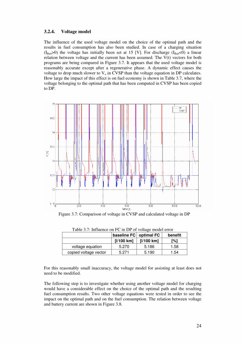
3.2.4. Voltage model The influence of the used voltage model on the choice of the optimal path and the results in fuel consumption has also been studied. In case of a charging situation (IBatt>0) the voltage has initially been set at 15 [V]. For discharge (IBatt<0) a linear relation between voltage and the current has been assumed. The V(t) vectors for both programs are being compared in Figure 3.7. It appears that the used voltage model is reasonably accurate except after a regenerative phase. A dynamic effect causes the voltage to drop much slower to Vo in CVSP than the voltage equation in DP calculates. How large the impact of this effect is on fuel economy is shown in Table 3.7, where the voltage belonging to the optimal path that has been computed in CVSP has been copied to DP.

Figure 3.7: Comparison of voltage in CVSP and calculated voltage in DP

Table 3.7: Influence on FC in DP of voltage model error

baseline FC optimal FC benefit [l/100 km] [l/100 km] [%]

voltage equation 5.270 5.186 1.58 copied voltage vector 5.271 5.190 1.54

For this reasonably small inaccuracy, the voltage model for assisting at least does not need to be modified. The following step is to investigate whether using another voltage model for charging would have a considerable effect on the choice of the optimal path and the resulting fuel consumption results. Two other voltage equations were tested in order to see the impact on the optimal path and on the fuel consumption. The relation between voltage and battery current are shown in Figure 3.8.

25

Figure 3.8: a) Initial voltage model for charging b) Linear voltage model for charging c) Quadratic voltage model for charging As it turned out, a different voltage model did not change the choice for the optimal path. Dynamic Programming still shows that only charging due to regenerative braking is beneficial and generating more than the powernet load is not, independent of the voltage model for charging. The optimal fuel consumption is given in Table 3.8 for the different voltage models and as can be seen, the effect on the FC is minimal, because the trajectory remains the same and no regular charging is ever applied. In case of regenerative braking, all models charge at 15 [V] and the model for discharging the battery is the same for all voltage models.

Table 3.8: Influence of different voltage models for charging on FC voltage model optimal FC

[l/100 km] constant voltage 5.1860

linear voltage 5.1858 quadratic voltage 5.1856

26

3.3. Conclusions Dynamic Programming has been used as a method to determine what the maximum fuel consumption benefit can be if the cycle is known beforehand. First simulations have been performed with different ISG's with a constant efficiency of 70, 80, 90 and 100 [%] efficiency. At higher efficiency, more charging and discharging will be performed, but that did not clearly influence the obtainable benefit. Next, a real 36 [V] ISG map had been downscaled to fit the 12 [V] system and although the chosen optimal trajectory for IBatt(t) was different, the obtained fuel consumption benefit was again about the same. As it turned out, increasing the electric load changed the optimal path, but the achieved fuel consumption benefit did not significantly change. The impact of the used grid size on the FC saving has also been studied and the conclusion is that decreasing the vertical grid size beyond a certain point on the NEDC cycle did not result in a further increase in FC benefit at the expense of a lot more computing time. Initially a simplified relation between the voltage and current was assumed and used for optimization. Fuel consumption results for the optimal path with this model and the computed, somewhat more realistic, voltage model from CVSP were compared and the difference in fuel consumption was relatively small. The influence on the choice of the optimal trajectory for two other voltage equations has also been researched and the conclusion was that the optimal path does not change for either of the other charging models. As a result, the fuel consumption remained about the same. In conclusion, the maximum obtainable fuel consumption benefit lies between 1.5 and 2.0 [%] for a 12 [V] system with a battery charge acceptance of 100 [A]. Since most of this benefit is due to regenerative braking, the charge acceptance is an important factor. The relation between charge acceptance and fuel economy will be researched later on.

27

Chapter 4

Control strategies In the previous chapter, the maximal possible benefit has been determined with a known cycle. The goal of the control strategies described in this chapter is to approach this benefit online. In order to accomplish this, the CVSP model is altered to allow power assist by a small electric power source, the ISG. Two different control strategies will be implemented, a heuristic and an analytical one. Aside from power assist, regenerative braking and stop-start are also included and the possible benefit of all these features will be determined. The control strategies are implemented in the master controller of the Simulink CVSP model. The task of a good control strategy is to recognize when it is economical to deliver electrical power and if so, how much assisting power would be optimal at each point in time. In combination with the charging strategy, it can also distinguish optimal points in time when to charge and at what rate. In other words: the strategy calculates the optimal electrical current in the master controller and sends it to the ISG, see Figure 2.2. 4.1. Heuristic control strategy In order to develop a functioning heuristic strategy, the optimal path that has been calculated by DP is compared to various vehicle signals. These signals could be for instance engine output power, vehicle acceleration, engine torque, engine speed and vehicle speed. The idea is to create a rule based strategy that will decide, based on correlations between the optimal current from DP and one or more of these signals whether to charge, assist or do nothing. The magnitude of the current should also follow out of the correlation. Since the optimal path for an electric load of 20, 30 and 40 [A] resemble each other closely, the choice has been to base the heuristic strategy on the IBatt vector of the 40 [A] powernet load (instead of on the path of the 10 [A] vector). After an observation of the different signals from DP a clear correlation between acceleration and the current can be observed in Figures 4.1a and b. The torque, power and throttle position signals are of course highly related. This means that there are also correlations between the above mentioned variables and the optimal current. Because the acceleration might be easier to actually measure in the vehicle, the combination of engine speed, acceleration and vehicle speed are preferred as system parameters for the heuristic strategy above torque and power.

28

Figure 4.1 a) Optimal path for 40 [A] load on the NEDC cycle b) Vehicle acceleration on the NEDC cycle

Acceleration Every time the vehicle accelerates, DP chooses for power assist. Therefore, in the heuristic strategy, assist will also be applied whenever the vehicle accelerates. The choice was made to make the level of assist proportional to the level of acceleration. In order to avoid oscillating behaviour due to 'hovering' of the acceleration around the activation value, a relay switch is used in the Simulink model of the control strategy. Based on the found correlation the relation between acceleration and the optimal current had to be split into two separate regions, above and below a certain vehicle speed. Deceleration It can be observed from Figure 4.1 that Dynamic Programming chooses the maximum charging current possible when the vehicle decelerates. As mentioned before, this is as expected, because obviously it is beneficial to store as much kinetic energy from the decelerating vehicle as possible in the battery. The heuristic relation between deceleration and the current is therefore a simple one: as soon as the vehicle's acceleration drops below a certain threshold, the strategy applies the maximal charging current possible. Alternatively, the current could also be linked to the throttle position. Normally, that would be an easier choice, but in this case the acceleration has to be measured anyway. In terms of FC benefit, the difference between both options is very small. Constant speed Unfortunately, when the speed is constant, after analysis of results obtained from the NEDC cycle, there seems little logic between the optimal path and the vehicle speed. There does appear to be some correlation between the engine speed and the optimal

29

current. However, a more advanced strategy is required in order to understand the decisions that DP makes for the optimal path. This strategy will be presented in paragraph 4.2. For now, the limited correlation between engine speed and current is used for the next rule. Based on the findings in the NEDC cycle, DP chooses to apply assist in situations where the engine speed is relatively low. Above a certain threshold, assist is never applied. Until this threshold is reached, the amount of assist is linear to the engine speed. The lower the engine speed, the higher the applied current. The reason behind this decision from DP to assist at a low engine power must be because of the low efficiency of the engine operating in that area of the specific fuel consumption map. By assisting at a low engine power, the amount of lost energy will be minimized. 4.1.1. Strategy results Based on the conclusions regarding the relation between the optimal current, the vehicle's acceleration, speed and the engine speed, the strategy rules given in Table 4.1 will be investigated.

Table 4.1: Heuristic control strategy rules

To be certain the vehicle is accelerating or decelerating, c1 and c2 are set respectively slightly above and below 0. For c2 a relay switch is used. In case the vehicle is accelerating, there should be power assist, so c4 and c5 should be negative. In order to make an estimation for c4 and c5, data from v, a and Iopt from the NEDC cycle are collected and the average values calculated. When the vehicle is decelerating, the charging current should be the maximal possible. It will be limited either by the charge acceptance of the battery plus the level of the powernet load or by the maximal possible current the ISG can generate, whichever is the bottleneck. The final rule before simulating can commence is to implement some sort of SOC correction in order to prevent SOC drift. The choice is made to use a polynomial as variable correction factor (cf) as a function of the SOC, which will be multiplied with the current calculated by the strategy. Multiple polynomials are possible to correct the current if necessary. In Figure 4.2 some possibilities for correction are given. The corresponding polynomials are given by:

1)SOC(SOC

)SOC(SOC(t))(

targmax

targ +−−

=i

i

tcf , (3)

with 1,3,5,7=i for (a), (b), (c) and (d) respectively The difference lies in the amount of tolerance that will be given to the system to deviate from the target SOC. The simulations will be done with the correction factor shown by

30

(b), because with this factor a moderate tolerance of a few percent deviation of the target SOC is given. Should this margin be exceeded, the system gradually increases or decreases the applied current. Because no regular charging will be applied, the correction factor will only be used to control the level of assist.

Figure 4.2: Possible relations between the correction factor and the SOC After simulating, a few slight modifications had to be made to the strategy rules in order to get a better resemblance between the optimal trajectory form CVSP and the trajectory from the heuristic strategy.

• A threshold for a minimal ICE torque was added for constant vehicle speed. Below this torque, the battery current equals zero.

• A threshold for a minimal required engine speed has been set in case of an accelerating vehicle. Otherwise, the battery current again equals zero.

After these modifications, the results matched the optimal path from DP already quite well for the NEDC cycle, but there was a slight deviation in SOC at the end of the cycle. For real world driving situations this is acceptable, but for an honest comparison in fuel consumption reduction, some fine-tuning had to be done in order to accomplish

0=∆SOC . The final values for all used parameters in the heuristic strategy are given in appendix D. The final path of IBatt(t) given by the heuristic control strategy and the optimal path from DP (grid size 2 [A] by 1 [s]) are both given for a 40 [A] electric load in Figure 4.3 and it can be seen that the trajectories match well.

31

Figure 4.3 a) IBatt(t) from model with heuristic control strategy for NEDC cycle

b) Optimal path for IBatt(t) as computed by DP for NEDC cycle The fuel consumption values calculated with the CVSP model are very close for the NEDC cycle. They are given in Table 4.2. Table 4.2: Comparison of FC of heuristic strategy with FC of optimal path for an electric load of 40 [A]

baseline FC optimal FC benefit [l/100 km] [l/100 km] [%]

optimal path from DP 5.276 5.177 1.9 heuristic PA trajectory 5.276 5.173 2.0

This means that at least for the NEDC cycle with an electric load of 40 [A], the heuristic control strategy functions very well. In fact, it functions even better than the optimal trajectory. The reason for this is that DP only investigates a certain number of trajectories, because the grid size is not infinitely small. If it could be set much smaller, the benefit could be slightly increased. Another consequence of the limitations of the current grid size is that the clutch might be open in CVSP, while DP cannot recognize this. This will also result in a slight reduction in fuel consumption when the optimal vector is exactly copied to CVSP. Although the results are promising, this does not necessarily imply that this strategy functions well in all driving cycles. The next logical step is to test the heuristic control strategy on other drive cycles. The two chosen speed profiles are the EPA city and the EPA highway cycle and again the optimal path as computed by DP and the path from the heuristic control strategy have been compared. The velocity profiles of the cycles are shown in appendix E and the optimal path and the heuristic path for IBatt(t) (for an electric load of 40 [A]) are also displayed there. For the online strategy it is the objective to be tuned in such a way that a charge balance is accomplished on the NEDC cycle. With the used values for the parameters c1

32

to c11, it is obvious that a charge balance will not be realized on any random cycle. Instead, the SOC has been restricted via the correction factor to always remain in the specified window of:

≤− targ)( SOCtSOC 5 [%] (4)

FC results of the simulations that have been run on the different cycles with a 10 [A] and 40 [A] electric load are shown in Table 4.3 and 4.4 respectively.

Table 4.3: FC results in CVSP for different speed profiles with 10 [A] load

cycle type NEDC EPA CITY EPA HWY FC / �SOC benefit FC / �SOC benefit FC / �SOC benefit [l/100 km] / [%] [%] [l/100 km] / [%] [%] [l/100 km] / [%] [%]

baseline 4.959 / +0.0 - 5.316 / +0.0 - 4.384 / +0.0 - optimal 4.878 / +0.0 1.6 5.243 / +0.0 1.4 4.367 / +0.0 0.4 heuristic 4.891 / +0.0 1.4 5.248* / +0.0 1.3 4.372* / +0.0 0.4

5.281** / +2.7 0.7 4.372** / +0.1 0.3

Table 4.4: FC results in CVSP for different speed profiles with 40 [A] load cycle type NEDC EPA CITY EPA HWY

FC / �SOC benefit FC / �SOC benefit FC / �SOC benefit [l/100 km] / [%] [%] [l/100 km] / [%] [%] [l/100 km] / [%] [%]

baseline 5.276 / +0.0 - 5.622 / +0.0 - 4.511 / +0.0 - optimal 5.177 / +0.0 1.9 5.530 / +0.0 1.6 4.488 / +0.0 0.5 heuristic 5.173 / +0.0 2.0 5.529* / +0.0 1.7 4.491* / +0.0 0.5

5.567** / +2.7 1.0 4.492** / +0.1 0.4 *Corrected fuel consumption so 0=∆SOC has been accomplished **Fuel consumption without correction, so 75≠endSOC [%] Because 0≠∆SOC on both EPA cycles, the cycles had to be tuned individually by multiplying the amount of delivered assist with a constant factor. Changing the amount of assist is a realistic way of correcting for SOC∆ , because this is what would occur by the SOC correction factor when the SOC would drift to far from the target SOC. After some testing on different cycles, it can be concluded that the strategy does not follow the optimal path that has been chosen by DP on the EPA cycles (see appendix E). An explanation for this must be that the used correlations are different when another cycle is being driven. However, fuel consumption reductions for the other tested cycles seem still very close to the optimum at first sight. The reason for this is that most of the benefit has to be attributed to regenerative braking. When the benefit is separated into the reduction due to regenerative braking and the reduction due to power assist, it becomes clear that the heuristic strategy does not function well at all. The results are displayed in Table 4.5. The benefit of power assist has been calculated by comparing the heuristic strategy, which includes regenerative braking and power assist, with a strategy that includes only regenerative braking. The initial difference between SOCtarg and SOCend by the regenerative strategy has been corrected by a constant discharge of the battery in all non braking phases so that charge balance is satisfied on all cycles and loads. The difference in FC between the heuristic and regenerative strategy is the saving due to assist.

33

Table 4.5: FC benefit due to power assist and regenerative braking for different electric loads with the heuristic strategy

cycle type elec. load total benefit benefit assist benefit regen. braking [A] [%] [%] [%]

NEDC 10 1.37 -0.26 1.63 40 1.94 0.14 1.80

EPA CITY 10 1.29 -0.24 1.53 40 1.64 -0.34 1.98

EPA HWY 10 0.28 -0.11 0.39 40 0.43 -0.03 0.46

34

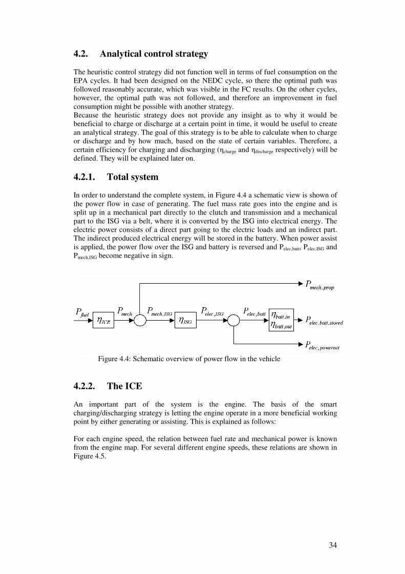
4.2. Analytical control strategy The heuristic control strategy did not function well in terms of fuel consumption on the EPA cycles. It had been designed on the NEDC cycle, so there the optimal path was followed reasonably accurate, which was visible in the FC results. On the other cycles, however, the optimal path was not followed, and therefore an improvement in fuel consumption might be possible with another strategy. Because the heuristic strategy does not provide any insight as to why it would be beneficial to charge or discharge at a certain point in time, it would be useful to create an analytical strategy. The goal of this strategy is to be able to calculate when to charge or discharge and by how much, based on the state of certain variables. Therefore, a certain efficiency for charging and discharging (�charge and �discharge respectively) will be defined. They will be explained later on. 4.2.1. Total system In order to understand the complete system, in Figure 4.4 a schematic view is shown of the power flow in case of generating. The fuel mass rate goes into the engine and is split up in a mechanical part directly to the clutch and transmission and a mechanical part to the ISG via a belt, where it is converted by the ISG into electrical energy. The electric power consists of a direct part going to the electric loads and an indirect part. The indirect produced electrical energy will be stored in the battery. When power assist is applied, the power flow over the ISG and battery is reversed and Pelec,batt, Pelec,ISG and Pmech,ISG become negative in sign.

Figure 4.4: Schematic overview of power flow in the vehicle 4.2.2. The ICE An important part of the system is the engine. The basis of the smart charging/discharging strategy is letting the engine operate in a more beneficial working point by either generating or assisting. This is explained as follows: For each engine speed, the relation between fuel rate and mechanical power is known from the engine map. For several different engine speeds, these relations are shown in Figure 4.5.

35

Figure 4.5: Relation between ICE’s mechanical power and fuel rate

It can be seen that mechPf

∆∆

is not linear. In the analytical control strategy, �f is used as

the difference in fuel consumption between 2 situations. In the first situation the current to the ISG is zero, in other words no charging or discharging takes place, the coordinates of a certain working point in Figure 4.5 are for instance (f2,P2). In the second situation the ISG is either generating or assisting (so 0≠ISGI ), which shifts the operating point on the fuel rate line, respectively to the right (for example (f3,P3)) or left (for example (f1,P1)). The total torque produced by the ISG and the ICE combined always remains the same at a certain point in time, whether a choice is made for charging, discharging or neither. �Pmech is the difference in mechanical power of the ICE as a result of the produced power of the ISG. �Pmech can be positive or negative, depending on whether the ISG is charging or discharging respectively. So at a constant engine speed, at a certain power level, it might be economical to either deliver power assist or to charge the battery,

depending on mechPf

∆∆

. This information is used in the model and the optimal assisting

or generating torque is continuously calculated. Obviously, the charging strategy has been altered in order to generate energy when it is 'cheap' to do so. Since the SOC must also have some influence on the strategy, the same correction factor is used as in the heuristic strategy. Each unit of fuel mass releases a certain amount of energy when burned, which can be shown by:

HfPfuel ⋅= (5)

In this formula H is a constant, called the lower heating value. The extra amount of fuel burned per unit of time for charging can thus be converted to an equivalent amount of power:

HfPfuel ⋅∆=∆ (6)

36

4.2.3. The ISG The ISG can convert electrical energy into mechanical energy and vice versa as mentioned before. This conversion occurs at a variable efficiency, which is dependent on the torque and ISG speed. The map given in Figure 3.4 is used in the model. For the efficiency of the ISG in case of generating and power-assisting, the formulas (7) and (8) are used respectively.

ISGISG

ISG

ISGmech

ISGelecgenISG T

IVP

P

ωη

⋅⋅

==,

,, , for IISG, TISG > 0 (7)

ISG

ISGISG

ISGelec

ISGmechastISG IV

TP

P

⋅⋅

==ωη

,

,, , for IISG, TISG < 0 (8)

4.2.4. The battery

The battery efficiency is defined as inin

outout

inbattelec

outbattelec

in

outbatt IV

IV

P

P

PP

⋅⋅

===,,

,,η (9)

Because in

out

I

I, known as the coulombic efficiency �C, has been set at 100 [%] in the

CVSP model, it shall also be set at 100 [%] in the analytical strategy. This simplifies the battery efficiency to:

in

out

inbattelec

outbattelecbatt V

VP

P==

,,

,,η (10)

With the knowledge that io RIVV ⋅+= for discharging, it is obvious that the highest efficiency is obtained when the battery is slowly discharged. Because the model should take into account that the battery's efficiency is dependent on the magnitude of the current for both generating and assisting, it is chosen to split up the efficiency into 2 parts, see Figure 4.6.

Figure 4.6: Battery power flow

The first partial efficiency is defined as:

in

o

inbattelec

storedbattelecinbatt V

VP

P==

,,

,,,η (11)

37

It is relevant for the generating part of the strategy, which will be discussed in the next paragraph. The second partial efficiency, required for the discharge part of the strategy as explained later on, is:

o

out

storedbattelec

outbattelecoutbatt V

VP

P==

,,

,,,η (12)

A combination of both efficiencies again leads to the more common definition of battery efficiency:

in

out

o

out

in

o

storedbattelec

outbattelec

inbattelec

storedbattelecoutbattinbattbatt V

VVV

VV

P

P

P

P=⋅=⋅=⋅=

,,

,,

,,

,,,, ηηη (13)

4.2.5. Charging In order to quantify whether generation is favourable, the dimensionless �charge (charging efficiency) is introduced. It is defined as:

Hff

PP

Hf

P

P

P powernetelecstoredbattelecuseful

t

usefulcharge ⋅−

+=

⋅∆∆

=∆∆

=)( 23

,,,

cos

η (14)

Here, �f is the amount of extra fuel the engine has to burn per unit of time and �Puseful is the extra amount of useful power, which consists of the power going to the powernet load and the power that is stored in the battery. In order to calculate the relation between the energy stored in the battery and the amount of extra fuel required all necessary efficiencies, as described above, have to be taken into the equation. With the formulae:

inbattelecinbattstoredbattelec PP ,,,,, ⋅= η , (15)

powernetelecISGelecinbattelec PPP ,,,, −= (16)

and equation (7), this can be rewritten as:

Hff

PP

Hf

P powernetelecinbattISGmechgenISGinbattusefuelcharge ⋅−

−+⋅⋅=

⋅∆∆

=)(

)1(

23

,,,,, ηηηη (17)

The generating strategy will thus try to maximize the amount of stored energy at the expense of energy inserted to the system in the form of extra fuel.

38

4.2.6. Discharging For discharging the battery, another definition has been chosen, because in case of power assist, fuel is not sacrificed in order to gain electric energy, but fuel is saved at the expense of electric energy. In case of assisting, the strategy must thus try to maximize the ratio of the fuel reduction over the amount of stored energy in the battery that is used for this saving. The used variable will be called �discharge (discharging efficiency) and is defined by:

storedbattelec

powernetelec

t

powernetelec

t

usefuldischarge P

PHff

P

PHf

P

P

,,

,21

cos

,

cos

)( +⋅−=

∆+⋅∆

=∆∆

=η (18)

Due to substitution of:

outBatt

outbattelecstoredbattelec

PP

,

,,,, η

= , (19)

powernetelecISGelecoutbattelec PPP ,,,, −= (20)

and equation (8), formula (18) can be rewritten as:

powernetelecoutbatt

ISGmechastISGoutBatt

powernetelecdischarge

PP

PHff

,,

,,,

,21

11

)(

��

�

�

��

�

�−�

�

�

�

��

�

�

⋅

+⋅−=

ηηη

η (21)

Here, f1 < f2 and �Pused < 0, so �discharge is positive in sign. 4.2.7. Strategy results On each time sample �charge and �discharge are computed for an array of possible ISG currents. Looking at the results for a certain random cycle, it can be noticed that the shape of �charge(t) and �discharge(t) are very similar for the different ISG currents ranging in this case from 10 to 110 [A] for charging and –450 to –10 [A] for assisting respectively. For discharging, this resemblance has been illustrated in figure 4.7 for a few random assist currents. Therefore, it seems to be a good idea to reduce complexity and take the magnitude of the ISG current out of the equation. To do this, the average of �charge and �discharge for different ISG currents will be taken. Alternatively, it would also be possible to make efficiency calculations with only one ISG current.

39

Figure 4.7: �discharge(t) for assist current of -10, -50, -90 and -150 [A]

The different efficiencies are compared with an average value over time for respectively �charge and �discharge. During the first period of the cycle, the averages for (dis)charging are set at a certain initial value, while the system is gathering information for the average values. After some time, the thresholds based on collected data will become reliable enough and will be triggered. In order to maximize the benefit for homologation (a standardized test procedure for measuring fuel consumption), the switch can be operated after the NEDC cycle has passed, for instance at 1500 [s]. Generation or power assist is performed when respectively equation (22) or (23) is met.

AVSchargeAVSchargecharge tt ,, )()( ηηη ∆+> (22)

AVSdischargeAVSedischargdischarge tt ,, )()( ηηη ∆+> (23)

In these equations, ��charge,AVS and ��discharge,AVS refer to added offsets. The physical meaning of these offsets is to compensate for the lost energy by the counterpart. For instance, the activation threshold for assist should be higher than the calculated average value, because the extra energy needed in the battery for the assist phase will be generated at a certain efficiency, which has to be taken into account in the decision whether it is beneficial to assist or not. Charging more than the powernet load means that this surplus on battery energy has to be discharged at some point, which also

40

occurs at a certain efficiency. In Figure 4.8, �discharge(t) and �discharge,AVS(t) are illustrated. Note that there is clearly a relation between �discharge(t) and the optimal trajectory as calculated by DP, shown in figure 3.6b. The surplus of energy from the battery is dissipated most economically during acceleration phases or in some constant speed phases. Power assist during deceleration phases is clearly not efficient as is logically expected.

Figure 4.8: Speed profile and discharging efficiency (�discharge) for the NEDC cycle The choice has been made to make the magnitude of the current in case of charging or discharging proportional to the difference between �charge or �discharge and the average value plus the offset. In formulae this yields:

=∆+−⋅= ))(( ,, AVSdischargeAVSdischargedischargedischarge kI ηηηdischarge

dischargedischargek η∆⋅ (24)

and

chargechargeAVSchargeAVSchargechargecharge kkI ηηηη ∆⋅=∆+−⋅= ))(( ,,charge (25)

for discharging and charging respectively. The 'cheaper' it will be, the more the strategy will (dis)charge. This is realized by the proportionality between the current and ��.

41

It turned out that the threshold for generation has to be set so high, that normal charging never takes place. Only charging due to regenerative braking is beneficial, which is consistent with the optimal path Dynamic Programming showed. Because kdischarge and ��discharge,AVS are the 2 remaining degrees of freedom that influence �SOC, an infinite amount of possibilities are possible for these 2 variables. If the NEDC cycle is chosen to accomplish �SOC, a number of possible values for the assist threshold have been investigated. Once an offset is selected, kdischarge is automatically set. With a high threshold, the strategy will assist rarely and with a high magnitude of the current. As the threshold gets lower, assist will become more frequent and the degree of assist less. Multiple options have been considered on 3 different cycles and although results were reasonably close, a setting of 1.1 for the threshold gave the best results, although the difference in FC between the investigated options was small (Table 4.6). Table 4.6: Tuning results for different thresholds and different values for Kdischarge

cycle NEDC EPA CITY EPA HWY average el. load 10 [A] 40 [A] 10 [A] 40 [A] 10 [A] 40 [A]

threshold FC FC FC FC FC FC FC

[l/100 km]

[l/100 km]

[l/100 km]

[l/100 km]

[l/100 km]

[l/100 km] [l/100 km]

1.5 4.893 5.193 5.233 5.539 4.369 4.492 4.891 1.4 4.888 5.175 5.226 5.506 4.369 4.489 4.881 1.3 4.886 5.174 5.228 5.503 4.367 4.489 4.880 1.2 4.884 5.174 5.228 5.501 4.366 4.489 4.880 1.1 4.884 5.174 5.228 5.499 4.365 4.489 4.879 1.0 4.885 5.174 5.228 5.498 4.366 4.489 4.880

In case both equations (22) and (23) are met, the strategy should choose charging or discharging, depending on the current SOC. If the SOC is higher than the target SOC, discharging should be performed and vice versa. However, since no normal charging is applied, equation (22) and (23) will never be met at the same time. In regenerative braking phases charging is always prioritised over assist. Furthermore, the same correction factor is used in order to avoid SOC drift. In this strategy it is again multiplied with the assist current. Regenerative breaking is always performed with the maximal current possible, even if it means crossing the upper SOC boundary. The only situation possible for this situation to occur is when the vehicle is descending a hill and the driver is continuously braking on the engine. In that situation, the battery could charge until the 100 [%] SOC is reached. Since the regenerative energy is always for free, this is a desired effect, even if this means that the SOC boundary will be breached. Simulations have been run and the fuel consumption results and the possible benefits are compared with the optimal trajectory from Dynamic Programming. The results are displayed in the Tables 4.7 and 4.8 for an electric load of 10 and 40 [A] respectively.

42

Table 4.7: FC results in CVSP for different speed profiles with a 10 [A] load cycle type NEDC EPA CITY EPA HWY FC / �SOC benefit FC / �SOC benefit FC / �SOC benefit

[l/100 km] / [%] [%] [l/100 km] / [%] [%] [l/100 km] / [%] [%] baseline 4.959 / +0.0 - 5.316 / +0.0 - 4.384 / +0.0 - optimal 4.878 / +0.0 1.6 5.243 / +0.0 1.4 4.367 / +0.0 0.4

analytical 4.884 / +0.0 1.5 5.228* / +0.0 1.7 4.365* / +0.0 0.4 5.254** / +1.7 1.2 4.357** / -0.9 0.7

Table 4.8: FC results in CVSP for different speed profiles with a 40 [A] load cycle type NEDC EPA CITY EPA HWY

FC / �SOC benefit FC / �SOC benefit FC / �SOC benefit [l/100 km] / [%] [%] [l/100 km] / [%] [%] [l/100 km] / [%] [%]

baseline 5.276 / +0.0 - 5.622 / +0.0 - 4.511 / +0.0 - optimal 5.177 / +0.0 1.9 5.530 / +0.0 1.6 4.488 / +0.0 0.5

analytical 5.174 / +0.0 1.9 5.499* / +0.0 2.2 4.489* / +0.0 0.5 5.539** / +1.8 1.5 4.474** / -0.9 0.8

*Corrected fuel consumption so 0=∆SOC has been fulfilled **Fuel consumption without correction, so 75≠endSOC The optimal path on the NEDC cycle is compared to the trajectory that has been computed by the analytical strategy (Figure 4.9). The comparisons for the two EPA cycles are shown in appendix F. An electric load of 40 [A] has been assumed and the grid size in DP had been set at 2 [A] by 1 [s].

Figure 4.9 a) IBatt(t) from model with analytical control strategy for NEDC cycle

b) Optimal path for IBatt(t) as computed by DP for NEDC cycle From the compared paths for the 3 different cycles it can be concluded that the resemblance is obvious. The only clear difference is that the voltage peaks from the optimal paths in the EPA cycles are not noticeable in the trajectories from the analytical

43

strategy. This is an advantage, because voltage stability on board of the vehicle is guaranteed with this strategy, as the voltage never drops below 12 [V], except in case of cranking. The trajectory produced by the analytical strategy matches better with the optimal path on the EPA cycles than the heuristic strategy does. As a result, the fuel consumption reduction is also higher. The FC results of the analytical strategy compared to the optimal path from DP copied into CVSP are about the same or on some cycles (for instance the EPA city cycle) the analytical strategy performs even better. The reason for this is that the results from DP could be improved if the grid size could be set smaller. The strategy in CVSP operates at 100 Hz and therefore has a much faster response in case of for instance a regenerative braking phase. Using the relatively large grid size has the consequences that DP simply does not recognize the actual best route, because it only calculates a limited number of possibilities. It will for instance lead to situations where the clutch in CVSP will be opened, while the copied vector from DP prescribes assist or maximal charging, because of a regenerative braking event. As a result of this phenomenon a correction of approximately 0.25 [%] (-0.013 [L/100 km]) should be made on the fuel consumption reduction of the optimal result in the EPA city cycle. This value has been obtained by copying the DP vector to CVSP an implementing a restriction in clutch open moments. In order to compensate for the change in SOC, the amount of assist has to be varied by a slight change of Kdischarge. On the other 2 cycles, the losses due to the consequences of the different sample times on the clutch are negligible. Another consequence of the sample time of 1 Hz in DP is that the speed profile will not be followed as accurate as in CVSP, which will result in an offset in fuel consumption between CVSP and DP. Unfortunately, the limited performance of the used PC prevents the grid size from being set significantly smaller. Because the heuristic strategy has been designed on the NEDC cycle with a 40 [A] load, the paths of the heuristic and analytical strategy are both pretty similar to the optimal path, which in turn leads to little deviation in terms of the fuel consumption results. To get an idea of the order of magnitude of the energy levels of the ICE and ISG and the efficiencies of the ICE and ISG, Table 4.8 is presented.

44

Table 4.8: Energy levels and efficiencies of the ICE and ISG for a load of 40 [A] strategy 1* strategy 2** strategy 3***

IPN [A] 40 40 40 UICE,mech,pos [MJ] 5.72 5.51 5.52

UICE,fuel [MJ] 20.62 20.13 20.11 UISG,mech,pos [kJ] 844.3 865.4 881.3 UISG,mech,neg [kJ] 0 0 0 UISG,elec,pos [kJ] 595.6 636.1 641.8 UISG,elec,neg [kJ] 0 0 0 �ICE,avs [%] 27.73 27.38 27.46

�ISG,gen,AVS [%] 27.54 73.50 72.82 �ISG,ast,AVS [%] - - - �batt,in [%] 100 84.00 84.00 �batt,out [%] 100 98.20 97.62

*baseline **only regenerative braking ***regenerative braking & power assist The obtained fuel consumption reduction from the analytical strategy can be split up in how much of the saving is due to power assist and how much due to regenerative braking. This is displayed in Table 4.9. Table 4.9: FC benefit due to power assist and regenerative braking for different electric loads with the analytical strategy

cycle type elec. load total benefit benefit assist benefit regen. braking [A] [%] [%] [%]

NEDC 10 1.50 -0.13* 1.63 40 1.93 0.13 1.80

EPA CITY 10 1.66 0.13 1.53 40 2.18 0.20 1.98

EPA HWY 10 0.44 0.05 0.39 40 0.48 0.02 0.46

*Because the strategy is online and uses some assumptions, it is possible that the fuel consumption benefit could be slightly negative in some situations.

The FC reduction of power assist has been computed by comparing the analytical strategy, which includes regenerative braking and power assist, with a strategy that includes only regenerative braking. Charge balance is accomplished for all cycles and loads by tuning of Kdischarge. As can be seen in Table 4.9, the fuel consumption reduction due to power assist alone is better than the heuristic strategy showed (Table 4.5), but it is still very low. The main reason for this is the relation between the fuel rate and mechanical power. This relation

is shown in Figure 4.5 and as one can see, mechdP

dfis relatively constant for a constant

engine speed for this particular ICE, especially for the operating range in terms of propulsion power in the analyzed cycles. Since the amount of power lost in the ICE is much larger than the amount of power lost in the ISG and battery (Table 4.8), the gain in FC is mainly dependent on allowing the ICE to operate in a more economical

45

working point, rather than shifting the working point of the ISG. The amount of

variation in mechdP

df is therefore of critical importance on the amount fuel consumption

reduction that will be obtained. Because the ISG has to convert the electrical energy back into mechanical energy in case of assist, additional losses are created which will lead to an even further decrease of the benefit of assist. Other ICE maps have also been studied in order to find out whether the relatively

constant relation of mechdP

df only occurs at the used 2.0 L diesel engine or if it is a more

general problem. It turned out that the latter was the case. Furthermore, compromises have to be made in the strategy, because the strategy has to make the decision when to charge or discharge and by what magnitude online. If the cycle and the electric load are known beforehand, the choice for the activation threshold for power assist and the factor Kdischarge can be optimized for that specific cycle and electric load. Because the analytical strategy can be applied on any cycle and electric load, the choice for the activation threshold and Kdischarge are unavoidably less than optimal for most/all situations. However, the compromise of tuning is of much

smaller influence than the limited variation of mechdP

df.

4.2.8. Emissions The goal of both strategies is only based on reducing the fuel consumption while maintaining charge balance for the NEDC and keeping the SOC within a certain window for all other cycles. However, shifting the ICE's operating point also has a clear effect on the emissions. The exhaust of the most important emissions, NOx, CO, HC and PM (particles) have been calculated in the baseline strategy and in the analytical strategy for the 3 different cycles with a 10 and 40 [A] electric load. In Table 4.10 it can be seen that the exhaust of NOx and PM has been reduced in all simulations with an average of respectively 2.1 and 3.6 [%] with respect to the baseline charging strategy. Unfortunately, there was also a slight increase in the exhaust of CO and HC in most cases. However, these emissions are calculated after the engine, but before the catalytic converter, so after-treatment is possible. Because it is more expensive to reduce NOx with after-treatment, this is the critical factor. All other emissions can be catalysed relatively cheap. Because the analytical strategy has a positive effect on the exhaust of NOx and PM at the expensive of a slight increase in CO and HC (which can be counteracted relatively easy with a catalytic converter) it is argued that it is a good trade-off and is an added bonus on top of the fuel consumption reduction. Expanding the strategy in order to include emissions in the decision whether to charge or discharge will increase complexity and will result in a compromise between fuel consumption saving and reduction of the specified emissions. Choosing weight factors to express the relative importance of the fuel consumption reduction in comparison to the reduction of the different emissions will be an important assumption for the strategy to function. A difficulty may lie in the shape that the emission maps have. A key element in the analytical strategy is the simplification that could be made in terms of the relation between the magnitude of the current and the efficiency of (dis)charging. When it is beneficial to charge or discharge at a certain point in time, this will be more or less true for any magnitude of the charging or discharging current. In other words, the quantity of the current does not have a significant influence on the choice whether

46

to charge, discharge or do nothing. Therefore, an important simplification could be made in the current analytical strategy. It is possible that for the shape of the emission maps a similar assumption cannot be made, which will complicate the strategy considerably. Despite the mentioned difficulties, the shape of the emission maps could lead to a relatively high amount of emission reduction, so it might be worth investigating the potential. Reducing emissions lies outside the scope of this research, but will be recommended for further research. Table 4.10: Change in exhaust of different emissions by analytical strategy with respect to baseline charging emission NEDC NEDC EPA CITY EPA CITY EPA HWY EPA HWY AVS.

10 [A] 40 [A] 10 [A] 40 [A] 10 [A] 40 [A] [%] [%] [%] [%] [%] [%] [%]

NOx -2.4 -3.4 -2.2 -3.0 -0.8 -1.0 -2.1 PM -4.4 -5.3 -3.6 -4.6 -1.5 -1.9 -3.6 CO 0.7 -1.8 0.8 0.6 0.4 0.5 0.2 HC 1.7 -1.6 1.2 1.4 0.8 1.0 0.8

Looking at the reduction of emissions, it seems is a much better idea to use the smart charging and discharging strategy for this purpose, rather than for the reduction of fuel consumption. Alternatively, increasing the performance of the vehicle by increasing the accelerating potential is also a possibility for the smart strategy. It only makes sense to use the analytical strategy for a fuel consumption reduction if the engine is calibrated differently. In that case, the difference between cheap and expensive working points will be increased and there will be more to be gained. 4.2.9. Dual battery system Because most of the benefit is accomplished by regenerative braking, it seems worth investigating the benefit when the maximal charging power is increased. This can be accomplished in two ways. The first way is to increase the charge acceptance of the battery, by increasing the capacity of the battery. This will be described in the next paragraph. The second way is to increase the voltage of the electrical system. However, because the electric loads will still function at the original voltage level, a DC/DC converter will be required in order to downgrade the voltage to 12 [V]. A 12 [V] battery is also still connected to the system in order to guarantee voltage stability for the electric loads. Furthermore, it can also provide the required power for the key-off load. Because it is generally not used, the capacity of this battery can be decreased to approximately 20 Ah in order to reduce costs. Since the vehicle is classified as a mild-hybrid, increasing the voltage of the ISG to 36 [V] seems the logical choice (see Figure 1.1), because the electrical power of the ISG has to remain relatively small. A schematic representation of the electric circuit of the dual battery system is given in Figure 4.10. In this configuration, the 12 [V] battery is only used for voltage stability and can be much smaller than in the single voltage system. Since the 12 [V] is basically not used, the throughput of this battery will be zero in the simulations and the powernet load will be generated by the ISG at 36 [V] after which it is downscaled by the DC/DC converter. The charge acceptance of the 36 [V] battery is also used to be 100 [A], which would make the battery very large. This might cause some problems in terms of built in size and extra weight that may require

47

the battery to be repositioned. Because the charge acceptance is the same and the 12 [V] battery has no throughput, IBatt(t) shows the same trajectory as in figure 4.9b. The CVSP model has been adapted for the dual voltage system and small changes to the analytical strategy have also been made. All results for the dual battery system given in this paragraph are calculated with the adapted analytical strategy.

Figure 4.10: Dual battery system The regenerative potential of the dual battery system is much larger, because the ISG is operating at 36 [V], while the charge acceptance of the battery is unchanged at 100 [A]. In order to be able to fully exploit the increased regenerative performance of the battery, the ISG has been scaled up to a maximal power level of approximately 10 [kW]. A schematic of the ISG efficiency map is given in Figure 4.11.

Figure 4.11: 36 [V] ISG efficiency map

However, in the NEDC cycle the regenerative potential is not the bottleneck, but the relatively slow deceleration is for most braking phases. When the vehicle decelerates and no fuel is injected, the drag torque of the engine already generates a considerable part of the required braking power. The remaining part is then caused by the generating torque of the ISG (regenerative braking). If the required braking power is still not met, the mechanical brakes of the vehicle are used.

48

There are two main ways for the regenerative braking strategy to be applied in moderate deceleration phases. In the first possibility, the choice is made not to inject fuel during deceleration. This would automatically mean that the generating current in some situations will be less than the maximal generating current possible in order to prevent the vehicle from decelerating too fast. This possibility will be referred to as variant 1. In the second situation, the maximal possible generating power is applied during deceleration. This could mean in some situations that extra fuel needs to be injected in order to reduce the engine drag torque, so that the speed profile will still be followed. Otherwise, the vehicle would again decelerate too quickly. Obviously, with the battery charging more, more energy will be available for power assist in order to maintain charge balance. This possibility is called variant 2. Of course, a compromise between both different regenerative strategies can also be made, so injecting a little extra fuel, but not so much that the maximal possible generating current is reached. However, only the two extremes are investigated and compared here. The question which option is the most economical has been researched and as it turned out, injecting extra fuel during deceleration proved to be slightly more economical for both battery systems, see Tables 4.11 and 4.12. So, the cost of the extra injected fuel during braking is overcompensated by the fuel saving as a result of the extra amount of power assist that will be carried out during other driving phases. Figures 4.12a and 4.12b show the optimal current of the ISG for variant 1 and 2 respectively for a single battery system. The ISG currents for the dual battery system are displayed in Figures 4.13a and 4.13b. In both cases the powernet load equals 10 [A] at 12 [V]. However, because the ISG operates at 36 [V] in the dual battery system, only

6.31 ≈⋅⋅

−PN

DCDChigh

low IVV

η[A] has to be charged extra to supply the electric load.

In all simulations a charge balance is maintained by increasing or decreasing the amount of power assist as can be seen in the plots. It can be observed by comparing the plots in Figure 4.12 that the regenerative potential of the single battery system with the ISG operating at 12 [V] is already above the maximal available energy in most of the braking phases of the NEDC cycle. In order words, even for a single battery 12 [V] system, the relatively slow braking phases are the bottleneck for the benefit obtained by regenerative braking instead of the maximal possible charging power. For the dual battery system, the difference between the maximal ISG charging current is obviously even larger between both variants, see Figures 4.13a and 4.13b.

49

Figure 4.12: ISG current for single battery system in analytical strategy for variant 1 and 2.

Figure 4.13: ISG current for dual battery system in analytical strategy for variant 1 and 2. The results are given in Table 4.11 and 4.12, for the single and dual battery configuration respectively. The benefit of the dual battery system is also measured against the 12 [V] baseline strategy.

50

Table 4.11: Obtained fuel consumption and benefit for different regenerative braking variants for the single 12 [V] battery system on the NEDC cycle with analytical strategy

FC benefit [l/100 km] [%]

baseline 4.959 - variant 1 4.895 1.3 variant 2 4.884 1.5

Table 4.12: Obtained fuel consumption and benefit for different regenerative braking variants for the dual battery system on the NEDC cycle with analytical strategy

FC benefit [l/100 km] [%]

baseline 4.959 - variant 1 4.888 1.4 variant 2 4.882 1.6

Because injecting some fuel in order to be able to assure the maximal possible charge current is the more beneficial regenerative strategy for both battery systems, it is applied in the analytical strategy. The main reason why the benefit in the NEDC cycle for the dual battery system is lower as expected is the fact that only a small amount of kinetic energy is available due to the relatively slow deceleration in each braking phase. Therefore, it could be concluded that the full potential of the dual battery system is not utilised in the NEDC cycle. In addition, the DC/DC converter has to downgrade the powernet load from 36 to 12 [V], which takes place between 90 and 95 [%] efficiency. In simulations, a constant value of 93 [%] has been taken. In the single 12 [V] battery system, the powernet load is already generated at 12 [V], so no energy is lost there. Finally, the ISG size is increased by a factor of 3. This causes more losses in comparison to the downscaled ISG. In addition to the lower benefit, adding a DC/DC converter and a 36 [V] battery increases system cost and complexity. It should be noted that the added mass of the extra components has been assumed to be negligible on the total weight of the car. Simulations have also been run on the EPA city and highway drive cycles. Because of the faster deceleration in the braking phases of the EPA city cycle, the regenerative potential has been utilised more in this particular cycle compared to the NEDC cycle and the result is a clear increase in fuel consumption benefit compared to the benefit obtained by the single battery system on the EPA city cycle. The FC saving on the EPA highway cycle on the other hand is lower than the FC saving of the single battery system. This can be explained by the fact that there are relatively few deceleration phases on this cycle, so the increase due to regenerative braking is limited, while the added DC/DC converter and the larger ISG cost extra fuel. The results on both cycles are shown in Table 4.13.

51

Table 4.13: Fuel consumption and benefit of dual battery system on EPA city and EPA highway cycles

cycle type EPA CITY EPA CITY EPA HWY EPA HWY FC benefit FC benefit [l/100 km] [%] [l/100 km] [%]

baseline 5.316 - 4.384 - single battery system 5.228 1.7 4.367 0.4 dual battery system 5.185 2.5 4.371 0.3

4.2.10. Battery charge acceptance The second way to increase the regenerative potential is to enlarge the 12 [V] battery in order to enhance the charge acceptance. This way, the added cost of the converter and the 36 [V] battery can be avoided and the increase in complexity is also prevented. The relation between charge acceptance and fuel consumption benefit has been investigated and is illustrated in Figure 4.14 for all 3 cycles. In order to accomplish a charge balance with different charge acceptances, the amount of assist had to be varied by tuning of Kdischarge. The calculated values for the fuel consumption and the benefit can be found in appendix G.

Figure 4.14: Relation between charge acceptance of the battery and the obtained fuel consumption benefit with the analytical strategy on the single battery system for 3 different cycles Increasing the charge acceptance of the battery is a more effective way of optimizing the FC saving than altering the electric architecture to a dual voltage system. From Figure 4.14 it can be seen that the FC reduction will rise on all cycles with a clear trend. Power assist has been used in order to ensure a charge balance, but the extra benefit due to this feature is small (Table 4.9). The dual battery system only managed to get a significant increase in FC saving on a cycle with a high amount of regenerative braking phases, like the EPA city cycle. On the NEDC cycle, the extra FC reduction was very limited and on the EPA highway cycle an even lower FC benefit was found than on the single battery system with an equal charge acceptance of 100 [A]. The

52

reasons are the efficiency of the added DC/DC converter and the larger ISG. In addition, the increased complexity and cost of the dual voltage network can be avoided by increasing the charge acceptance. The only limitation in increasing the charge acceptance is the size of the ISG. For the (downscaled) ISG a charge acceptance of around 175 [A] is the maximum possible in order for the ISG to still be able to provide the electric load during a regenerative braking phase. 4.2.11. D-ISG configuration Another way to increase the possible FC benefit is by changing the vehicle's powertrain architecture to the D-ISG configuration as shown in Figure 1.4 (page 6). The key advantage of this layout is that the clutch can be opened during regenerative braking phases, which will result in a higher amount of kinetic energy to be converted to electric power. It should be noted that the D-ISG configuration prevents the ISG from generating when the velocity of the vehicle is zero, because the ISG is connected to the transmission and the speed on the input and output shafts are zero. This means a slight adaptation to the analytical strategy, so that the battery provides the powernet load when the vehicle is not moving. Cranking the ICE is different in this configuration than in the B-ISG design, because the clutch is located between the ISG and the ICE. When the velocity of the vehicle is zero, the clutch will be opened and therefore it cannot be used to crank the ICE. There are multiple options to solve this issue. One possibility is to install an additional start motor and another is to adapt the gearbox in such a way that is automatically geared in neutral when the ICE has to be started. With the adapted gearbox, the clutch can be closed without problems and cranking will be performed by the D-ISG. The final solution is to have a dual clutch system: one clutch before and one behind the D-ISG. Either options has its own advantages and disadvantages in terms of added complexity and add-on cost and further analysis (which lies outside the scope of this research) will be necessary to determine the best possibility. There are two possibilities for the ICE to behave when a deceleration event occurs and the clutch is opened. The ICE can either run on idle speed or it can be switched off. When the ICE is switched off during deceleration, a restriction is implemented in order to avoid a high emission increase. Cranking of a cold ICE causes a relatively high output of emissions and therefore a certain time is necessary to allow heating up of the ICE and catalytic converter, before the ICE can be switched on and off, so:

195__min_ => offonICEtt [s] (26)

The value of 195 [s] is an engineering estimate, which coincides with the completion of the first sub cycle within the NEDC cycle. Both options (ICE idling and ICE turned off during deceleration) have been explored and the fuel consumption reductions on the 3 different cycles for an electric load of 10 and 40 [A] are given in Table 4.14 and 4.15. The large difference in FC benefit between the 2 possible variants is explained below.

53

Table 4.14: FC results of analytical strategy on the different cycles for 2 different electric loads for the single and dual battery system with the ICE running at idle speed during deceleration

cycle type load baseline 12 [V] 36/12 [V] FC FC saving FC saving [A] [l/100 km] [l/100 km] [%] [l/100 km] [%]

NEDC 10 4.959 4.943 0.32 4.847 2.27 40 5.276 5.227 0.93 5.110 3.15

EPA CITY 10 5.316 5.289 0.51 5.152 3.09 40 5.622 5.546 1.34 5.398 3.98

EPA HWY 10 4.384 4.376 0.18 4.359 0.57 40 4.511 4.494 0.37 4.491 0.44

Table 4.15: FC results of analytical strategy on the different cycles for 2 different electric loads for the single and dual battery system with the ICE switched off during deceleration

cycle type load baseline 12 [V] 36/12 [V] FC FC saving FC saving [A] [l/100 km] [l/100 km] [%] [l/100 km] [%]

NEDC 10 4.959 4.776 3.68 4.697 5.28 40 5.276 5.066 3.98 4.947 6.24

EPA CITY 10 5.316 5.063 4.76 4.936 7.15 40 5.622 5.320 5.36 5.163 8.16

EPA HWY 10 4.384 4.338 1.05 4.321 1.44 40 4.511 4.456 1.22 4.453 1.28

In table 4.16 it can be noticed that the obtained benefit from power assist is still in the same order of magnitude as before. This means that the boost in FC reduction compared to the 12 [V] B-ISG system is obtained by a larger regenerative braking benefit. Table 4.16: FC reduction split up for 36/12 [V] dual battery system on the NEDC cycle for 10 and 40 [A] electric loads

electric load regen. braking power assist [A] [%] [%] 10 5.28 0.00 40 6.16 0.08

In the B-ISG configuration, the clutch is closed during deceleration, which results in a large portion of the kinetic energy to be absorbed by the ICE. Because the ICE provides a negative torque in this case, the amount of injected fuel will be less than the amount needed for idle speed.

54

So, during when the ICE is running on idle speed

0=ICET (27) and during deceleration

0<ÍCET (28)

with the clutch closed. The result is that:

decelidle ff > (29) When the ICE is decoupled during braking in the D-ISG powertrain, the ICE cannot provide a negative torque anymore and more energy can be absorbed by the electrical system. When the ISG delivers the maximal generating power, the remaining part of the kinetic energy will be dissipated by the mechanical brakes. So basically, in the D-ISG design more kinetic energy is dissipated by the brakes and ISG and no braking on the ICE is performed. However, in this situation fuel is still required in order to allow the ICE to idle. This required amount is more than the ICE would need when it is used as a brake (see formula 27) as in the B-ISG design. In fact, the amount of fuel required to maintain idle speed on the diesel ICE is approximately 30 [%] of the fuel required to drive the C-max at a constant speed of 50 [kph] in 4th gear on a level road. Therefore, it can be noticed that the fuel consumption benefit of the 12 [V] D-ISG is actually lower than the reduction achieved by the 12 [V] B-ISG when the ICE was programmed to idle during deceleration (compare Table 4.9 and 4.14). It should be noted that these results have been obtained with the same downscaled 12 [V] ISG map and battery have been used as before. The charge acceptance is also limited to 100 [A]. For the D-ISG configuration it is considered therefore absolutely necessary to shut down the ICE during deceleration. In that case 0=ICEf , but the ICE still does not provide a braking power. As a result, the fuel consumption reduction has been increased considerable for the ICE-off situation (compare Tables 4.14 and 4.15). In the B-ISG configuration, it is possible to inject extra fuel in order to increase TICE, in case the vehicle will decelerate too rapidly and the velocity profile is no longer followed. The maximal possible ISG generating current can thus be maintained. This proved to be slightly more economical than injected no extra fuel and charging less than the maximal amount possible. However, when the clutch is opened during braking in the D-ISG design, this is not possible, because no ICE power can be transferred to the wheels. Therefore, in case of very slow deceleration, the generating power of the ISG should always be limited to the available kinetic energy. In a formula this yields:

brakesmechISGICEprop PPPP ,++= (30)

In the D-ISG configuration during deceleration:

0=ICEP (31) and

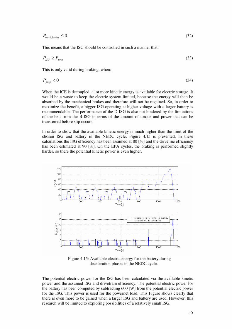
55

0, ≤brakesmechP (32)

This means that the ISG should be controlled in such a manner that:

propISG PP ≥ (33)

This is only valid during braking, when:

0<propP (34)

When the ICE is decoupled, a lot more kinetic energy is available for electric storage. It would be a waste to keep the electric system limited, because the energy will then be absorbed by the mechanical brakes and therefore will not be regained. So, in order to maximize the benefit, a bigger ISG operating at higher voltage with a larger battery is recommendable. The performance of the D-ISG is also not hindered by the limitations of the belt from the B-ISG in terms of the amount of torque and power that can be transferred before slip occurs. In order to show that the available kinetic energy is much higher than the limit of the chosen ISG and battery in the NEDC cycle, Figure 4.15 is presented. In these calculations the ISG efficiency has been assumed at 80 [%] and the driveline efficiency has been estimated at 90 [%]. On the EPA cycles, the braking is performed slightly harder, so there the potential kinetic power is even higher.

Figure 4.15: Available electric energy for the battery during deceleration phases in the NEDC cycle. The potential electric power for the ISG has been calculated via the available kinetic power and the assumed ISG and drivetrain efficiency. The potential electric power for the battery has been computed by subtracting 600 [W] from the potential electric power for the ISG. This power is used for the powernet load. This Figure shows clearly that there is even more to be gained when a larger ISG and battery are used. However, this research will be limited to exploring possibilities of a relatively small ISG.

56

Tests on the rollerdyno are necessary to investigate whether ICE shutoff during regenerative braking phases will not negatively influence the driveability of the vehicle too much. Of course, it would not make much sense to shut the ICE down during deceleration and than start it up again in the idle phase. Instead, it is more logical to integrate stop-start as well into the vehicle, so that the ICE is shut down in the deceleration phase and it is started up again when the vehicle accelerates, after the idle phase. Stop-start is explored in the next paragraph and the fuel consumption benefit for both the B-ISG and D-ISG design with stop-start implemented on top of regenerative braking and power assist has been calculated for the same cycles and loads. 4.3. Stop-start The final mild-hybrid feature that will be investigated is the possibility of stop-start. This simply means that during a vehicle standstill phase, the ICE is automatically shut down, when the gear is in neutral. When the driver wants to accelerate and presses the clutch pedal in order to select a gear, the ICE automatically starts up again. In the CVSP model this is easily implementable by switching the ICE when the following conditions are met:

• 1.0)( _min_ =< startstopvtv [ms-1] (35)

• 1)( _min_ =≤ startstopthrottletthrottle [%] (36)

• 60)( _min_ =≥ startstopSOCtSOC [%] (37)

• 195_min_ => startstoptt [s] (38)

The first 2 conditions are obvious, because the vehicle must be standing still and the acceleration must also equal zero. The restraint on the battery's SOC is implemented, because after each stop phase, the ICE has to be started up again, which will cause a drop in the powernet voltage. When the SOC decreases, Vo will also be lowered and therefore the situation might occur where the cold cranking voltage will be too low. For the analytical strategy, however, this restraint will have no influence, because the SOC correction factor will keep the SOC above 70 [%] under all normal driving circumstances. The only exception will be the situation where the vehicle is parked for a long time (multiple weeks) and the battery is slowly drained due to self-discharge and the key-off loads. Finally, the minimal amount of time that has to be elapsed since the initial ignition before stop-start can be applied has to be larger than 195 [s]. The reason for this limitation is the same as in the D-ISG configuration where the ICE is shut down during braking phases: the ICE needs to warm up before switching it on and off in order to avoid a large increase in emission output. In this paragraph the added FC benefit of stop-start on top of regenerative braking and power assist will be examined. Without stop-start, the analytical strategy always chooses to charge the powernet load in a vehicle standstill phase. With the ICE turned off, the ISG is not able to charge, because 0== ISGICE ωω , so the battery therefore has to provide the required power for the electric loads. In order to make stop-start compatible to the strategy, the amount of assist has to be slightly varied to accomplish charge balance. Furthermore, the additional cranking currents after the stop phases will also cause a slight decrease in SOCend in the order of ( 110− [%]). As a result of the extra cranking

57

currents and the extra drain on the battery during idle phases, a slightly lower setting of the tuning parameter Kdischarge is necessary in order to keep a charge balance on the NEDC cycle. The influence of stop-start on the fuel consumption benefit has been computed and 0=∆SOC on other cycles is again realized by tuning of the amount of assist by varying Kdischarge. Because the dual battery system did not provide attractive results for the B-ISG with respect to the extra add-on cost, stop-start is only evaluated for the single battery system in this layout. For the D-ISG, the benefit of stop-start on both the single and dual battery system has been determined. The results of stop-start on the B-ISG configuration are displayed in Tables 4.17 and 4.18 for 10 and 40 [A] electric loads respectively. Table 4.17: Obtained FC benefit from mild-hybrid features with B-ISG and analytical strategy on multiple drive cycles for an electric load of 10 [A]

cycle type baseline analytical benefit benefit benefit benefit [l/100 km] [l/100 km] [%] [%] [%] [%]

NEDC 4.959 4.657 6.08 1.63 -0.13 4.58 EPA CITY 5.316 5.060 4.82 1.53 0.13 3.16 EPA HWY 4.384 4.363 0.49 0.39 0.05 0.05

regen. braking X X X power assist X X X

stop-start X X X Table 4.18: Obtained FC benefit from mild-hybrid features with B-ISG and analytical strategy on multiple drive cycles for an electric load of 40 [A]

cycle type baseline analytical benefit benefit benefit benefit [l/100 km] [l/100 km] [%] [%] [%] [%]

NEDC 5.276 4.962 5.94 1.80 0.13 4.01 EPA CITY 5.622 5.335 5.10 1.98 0.20 2.92 EPA HWY 4.511 4.487 0.52 0.46 0.02 0.04

regen. braking X X X power assist X X X

stop-start X X X The FC consumption reduction of the D-ISG system with power assist, regenerative braking and stop-start has been displayed in Table 4.19. Obviously, these benefits are calculated on the variant where the ICE is shut down during deceleration. By comparing Tables 4.17, 4.18 and 4.19 it can be seen that the extra benefit of the added stop-start feature to the analytical strategy is practically the same for both the B-ISG and D-ISG layout for the single battery system.

58

Table 4.19: Obtained benefit from D-ISG configuration on multiple drive cycles with analytical strategy for single and dual battery system with stop-start included

cycle type load baseline 12 [V] 36/12 [V] FC FC saving FC saving [A] [l/100 km] [l/100 km] [%] [l/100 km] [%]

NEDC 10 4.959 4.554 8.16 4.477 9.71 40 5.276 4.844 8.19 4.734 10.27

EPA CITY 10 5.316 4.897 7.88 4.776 10.16 40 5.622 5.155 8.30 5.003 11.00

EPA HWY 10 4.384 4.336 1.10 4.319 1.48 40 4.511 4.455 1.24 4.452 1.30

4.4. Battery lifetime In the baseline strategy the ISG charges the powernet load, so the battery is not used, except for cranking and key-off loads, making the throughput almost zero. Other limiting factors for the battery life in that case are corrosion and loss of water due to gassing. These factors cause the expected lifetime of the battery to be in the order of 8 years. In the case of the analytical strategy, the battery is utilised for regenerative braking, power assist and stop-start. The throughput is therefore much higher, which unavoidably decreases the lifetime of the battery.

Figure 4.16: Number of cycles versus DOD for a flooded LA battery

It has been calculated that the charging throughput on the NEDC cycles is around 3.5 [Ah]. A realistic size for the battery with a charge acceptance of 100 [A] is at least 100 [Ah] (without pre-conditioning). This would make the throughput on the NEDC cycle

3.5 [%]. So, 1 battery cycle is completed on every 6.28035.01 ≈ NEDC cycles. Since

59

the DOD of the battery lies in the order of a few percent, the battery lifetime is approximately 145 cycles, see Figure 4.16. However, because of the high demands on the battery, it is unavoidable to use an AGM battery for the application of the hybrid vehicle. It is much more stable than a flooded LA battery and the lifetime of this battery compared to the flooded battery is approximately 3 times higher. Unfortunately it is also more expensive. This would mean that the lifetime of the AGM battery would be:

310137116.281453 ⋅≈⋅⋅⋅ [km]. Assuming an average driving distance of 31020 ⋅ [km]/year, the battery lifetime would be approximately 6 to 7 years. Obviously, this number has been calculated for the situation where the driver only drives NEDC cycles, and since the charging throughput is based on the amount of regenerative braking pulses, the lifetime could be different, depending on the amount of braking phases. 4.5. Conclusions It became obvious during the analysis of the results of the heuristic strategy that a simple heuristic strategy based on the relation of the optimal current from DP with the speed and acceleration of the vehicle was not able to provide good results in other situations than the NEDC cycle with an electric load of 40 [A]. Therefore, a closer look in the total system (the vehicle) was required in order to make a better judgement. This has been done with the design of the analytical strategy. The results of the analytical strategy were as good as the maximum possible results DP promises or on some cycles even better. The reason for this to occur is the different sample times of CVSP and DP. This leads to the loss of some of the FC benefit when the optimal IBatt(t) vector is copied from DP to CVSP. It has been calculated that 90 to 100 [%] of the obtained FC benefit from the analytical strategy has to be attributed to regenerative braking, depending on the cycle and electric load. The remaining part is caused by power assist. So for this particular diesel engine at least, the potential saving due to assist is better the heuristic strategy accomplished, but the reduction is still very

small. The reason for this is the limited fluctuation inmechPf

∆∆

for the diesel engine.

In addition to the FC saving, a positive effect of the analytical strategy on the exhaust of emissions has been observed. It seems worth investigating whether power assist can better be used with the eye on reducing emissions rather than on saving fuel. In order to increase the benefit, two options were investigated, namely increasing the charge acceptance of the battery and changing the electrical architecture to a dual battery system with a 36 [V] ISG. Simulations showed that the FC reduction with the dual battery system is not straightforward. On the EPA city cycle the benefit was increased significantly with respect to the single battery system, but on the EPA highway cycle the benefit was less. On the NEDC cycle a small extra saving was accomplished. A major disadvantage of changing to a dual battery system is the unavoidable increase in complexity and cost. The relation between charge acceptance and FC benefit showed that a higher charge acceptance will lead to a higher reduction on all three cycles without the extra complexity and with only a small increase in cost. The possible increase in charge acceptance is limited by the size of the ISG. The added benefit of stop-start in the vehicle will lead to a relatively high fuel consumption reduction on city cycles. On the EPA highway cycle the benefit is obviously very low.

60

Chapter 5

Conclusions and recommendations The purpose of this research was to investigate the fuel consumption reduction that can be obtained with different mild-hybrid features on a specified vehicle, such as smart charging and discharging, regenerative braking and stop-start with a belt driven ISG with a relatively small electric power level. An acknowledged vehicle model (CVSP), created by the Ford Motor Company has been used for validation. Although the CVSP model has been verified with respect to rollerdyno tests and is considered to be reasonably precise, it is recommended to model the charging part of the battery voltage more accurately. Another recommendation is to verify the obtained simulation results on a test bench in the test laboratory. 5.1. Dynamic Programming Dynamic Programming is a method that has been used to determine the possible FC benefit when the cycle is known beforehand. It created a grid of options to control the battery current, while achieving a charge balance between the beginning and end of the cycle. Not only does this method show the potential fuel consumption reduction, but from the chosen path an insight is obtained in when DP chooses to charge and discharge and by what quantity. The recommendations regarding DP are to use either a faster computer with more internal memory or a more efficient algorithm in order to be able to decrease the grid size, which would lead to more accurate results and a higher benefit. 5.2. Strategies and FC reductions of mild-hybrid features Two online strategies have been designed to approach the fuel consumption benefit of DP. The first is a heuristic strategy which is based on the correlation between the acceleration, speed and the chosen battery current by DP. The results of this strategy are close to the optimal trajectory from DP, but this is only because the main part of the benefit is due to regenerative braking and this reduction can be obtained quite easily. When the benefit is split up into a part power assist and a part regenerative braking, it turned out that the benefit of assist alone in the heuristic strategy is negative in most cases. Therefore, it was necessary to design an analytical strategy which determined a generating and assisting efficiency and selects charging or discharging when it is beneficial to do so from an energetic point of view. So on each point in time, the costs of charging and discharging are evaluated and a decision is made how to control the ISG. This strategy gave better results although the benefit due to power assist was still very low (in the order of 0.1 [%]). However, the reason for this lies in the relation between the fuel rate and the mechanical power level for a constant engine speed. In the operating range for the driven cycles, this relation is reasonably linear, which means that the benefit that can maximally be obtained is relatively low compared to other mild-hybrid features. Furthermore, when the ISG assists, electrical energy will be converted into mechanical energy. This will cause some extra losses, which have a negative impact on the benefit. It should be noted that several other ICE maps showed a similar linear relation between fuel rate and mechanical power in the operating power range for the driven cycles. A possibility to increase the benefit of the smart charging and discharging strategy is to modify the engine calibration for drivetrains that are

61

equipped with an ISG in order to generate a larger difference between 'cheap' and 'expensive' areas. Alternatively, it is stated that it the smart charging and discharging strategy can also be used for other purposes. One could think of for instance increasing the performance of the vehicle by increasing the accelerating potential or decreasing emissions rather than decreasing fuel consumption. For further research it can be recommended to investigate either of these options. The current strategy (based only on fuel economy) already proved to have a beneficial effect on the exhaust of NOx and particles at the expense of a light increase in exhaust of CO and HC. Since the after-treatment of NOx is the most difficult, this trade-off is considered a good one. Stop-start and regenerative braking must be used to provide the FC benefit. Regenerative braking delivers a benefit around 1.5 to 2.0 [%] on the NEDC and EPA city cycle for a 12 [V] B-ISG and around 0.4 to 0.5 [%] on the EPA highway cycle. Stop-start is an easily implementable mild-hybrid feature that has a considerable FC benefit in the order of 3 to 5 [%] on city cycles and approximately 0.05 [%] on the investigated highway cycle. The reason that the benefit of stop-start and regenerative braking on this cycle is relatively low is simply because the engine output power is high and the amount of braking and stop phases is low. 5.3. Dual voltage system and D-ISG Several possibilities have been analysed to enlarge the FC benefit. A dual battery system with a 36 [V] ISG was not able to get a significant increase in fuel consumption saving in combination with the B-ISG. Because the ICE provides most of the braking power required in the relatively slow braking phases in the prescribed cycle, the amount of kinetic energy available for regenerative braking is limited, resulting in the fact that the larger ISG and battery for the 36 [V] powernet cannot be fully utilised. Furthermore, there are some added losses due to the larger ISG and the DC/DC converter that is necessary to downscale the power to 12 [V] for the electric loads. Considering that the dual battery system definitely adds complexity and cost to the powertrain of the vehicle, it is certainly not recommended as a realistic option for a B-ISG. The bottleneck of the electric system is the charge acceptance of the battery. Increasing the charge acceptance is an easy way of increasing the FC reduction on all cycles. However, the added benefit must be weight up against the added cost, weight and volume of the larger battery. There is also a limit in increasing the battery before the ISG becomes the bottleneck. The solution to the limited amount of available electric energy is to relocate the ISG. Instead of a belt driven ISG, the ISG should be located on the transmission side of the clutch (D-ISG). This way, the braking torque of the ICE can be avoided, making more kinetic energy available for regeneration. When the clutch is opened during deceleration phases, the ICE can be run on idle or be completely shut down. Because the ICE consumes a relatively high amount of fuel in idle, shutting the ICE down is recommended in order to maximize the reduction. Since the potential of the dual battery system is exploited much more in this configuration, it is considered to be good possibility for a D-ISG system. For further research it is recommended to investigate different voltage levels for the primary circuit. The relation between voltage level and FC reduction can be investigated with the goal of finding an optimum in the ratio of benefit to add-on cost. 5.4. Battery lifetime The impact on battery lifetime is dependent of the charging (or discharging) throughput of the battery. Calculations of the throughput on the NEDC cycle with the ISG controlled by the analytical strategy showed that a battery lifetime of approximately 6

62

to 7 years is possible when an LA AGM battery is chosen with a capacity of 100 [Ah]. It can be concluded that a large AGM LA battery can meet the requirements and there is no need to resort to other, more expensive, battery types.

63

References [1] Langari, R., Won, J.S., "A Driving Situation Awareness-Based Energy Management Strategy for Parallel Hybrid Vehicles", Fuel Transportation Technology Conference Costa Mesa, California, 06-2003. [2] van der Graaf, R., Spijker, E., Kok, D., "Integration of Drive System, Subsystems and Auxiliary Systems of a Flywheel Hybrid Driveline with respect to Design Aspects and Fuel economy", VDI Berichte Nr. 1459, 02- 1999. [3] Lukic, S., "Effects of Drivetrain Hybridization on Fuel Economy and Dynamic Performance of Parallel Hybrid Electric Vehicles", IEEE transactions on vehicular technology, vol. 53, no. 2, 03-2004. [4] Kok, D., "Hybrid Electric Vehicles - Micro-Hybrids as a Step Towards Lower Emissions and Fuel Consumption", VDA Technical congress, 03-05. [5] Koot, M., Kessels, J., de Jager, B., "Fuel Reduction of Parallel Hybrid Electric

Vehicles", Vehicle Power and Propulsion Conference, 2005. [6] Van Dongen, A., "Development and implementation of smart charging

strategies in a starter/alternator vehicle", DCT-number: 2002-44, 06-2002. [7] Koot, M., Kessels, J., de Jager, B., Heemels, W., van den Bosch, P., Steinbuch,

M., "Energy management strategies for vehicular electric power systems", IEEE transactions on vehicular technology, vol. 54, no. 3, 05-2005.

[8] Lin, C.C., Peng, H., Grizzle, J.W., Kang, J.M., "Power management strategy for a parallel hybrid electric truck", IEEE Trans. on Control Systems Technology, 11(6):839–849, 11-2003. [9] Steinmaurer, G., del Re, L., "Optimal Energy Management for Mild Hybrid Operation of Vehicles with an Integrated Starter Generator", SAE World Congress Detroit, Michigan, 04-2005. [10] Han, Z.,Yuan, Z., Guangyu, T., Quanshi, C., "Optimal Energy Management Strategy for Hybrid Electrical Vehicles", SAE World Congress Detroit, Michigan, 03-2004. [11] Webpage: http://users.telenet.be/educypedia/electronics/componentbattery.htm [12] Ehsani, M., "Electrical System Architectures For Military Vehicles", IEEE- paper, 2004. [13] Denton, T., "Automotive Electrical and Electronic Systems", TU/e library, 1995. [14] Karden, E., Surewaard, E., Spijker, E., Kok, D., "Lead-Acid Battery Management in Future Vehicles", VRLA Traction 2005, Symposium in conjunction with AABC05, 06-2005. [15] Arnolds, M., "Series hybrid powertrain", DCT-number: 2005-26, 05-2005.

64

[16] Bertsekas, D.P., "Dynamic Programming and Optimal Control", Athena Scientific, Belmont, MA, 1995. [17] Scordia, J., Desbois-Renaudin, M., Trigui, R., Jeanneret, B., Badin, F., "Global optimization of energy management laws in hybrid vehicles using dynamic programming", International Journal of Vehicle Design, 39(4), 2005.

65

List of abbreviations AUX Auxiliary System BATT Battery CHA Chassis CVSP Corporate Vehicle Simulation Program DOD Depth of Discharge DP Dynamic Programming EPA Environmental Protection Agency FC Fuel Consumption FFA Ford Forschungszentrum Aachen HWY Highway ICE Internal Combustion Engine ISG Integrated Starter Generator LA Lead Acid MPV Multi Purpose Vehicle MSC Master Controller NEDC New European Drive Cycle PA Power assist PN Power Net PP Power Plant SOC State of Charge VERL Vehicle Emissions Test Laboratory

66

Symbols a acceleration [m/s2] A area [m2] cf correction factor [-] C capacity [Ah] Cw drag coefficient [-] f fuel rate [g/s] frol rolling resistance coefficient [-] g gravity coefficient [m/s2] H lower heating value [J/g] I current [A] IBatt battery current [A] Icharge charging current [A] Idischarge discharging current [A] IISG ISG current [A] IPN powernet current [A] kcharge amplification constant for charging [A/%] kdischarge amplification constant for discharging [A/%]

m mass [kg] Pelec,batt electric power to/from battery [W] Pelec,batt,stored stored electric power [W] Pelec,ISG electric power from ISG [W] Pelec,powernet electric power of powernet [W] Pfuel power of burned fuel [W] Pmech mechanical power [W] Pmech,ISG mechanical power of ISG [W] Pprop propulsion power [W] Puseful useful power [W] r radius [m] Ri internal resistance [VA] UICE,fuel energy of burned fuel in ICE [J] UICE,mech,pos positive mechanical energy delivered by ICE [J] UISG,elec,neg negative electrical energy delivered by ISG [J] UISG,elec,pos positive electrical energy delivered by ISG [J]

UISG,mech,neg negative mechanical energy delivered by ISG [J]

UISG,mech,pos positive mechanical energy delivered by ISG [J]

v speed [m/s] V voltage [V] Vo open circuit voltage [V] t time [s] tmin-ICE-on-off min. elapsed time before ICE can be switched on/off [s] tmin-stop-start min. elapsed time before stop-start can be applied [s] T temperature, torque [°C], [Nm] TISG ISG torque [Nm] � angle [°] � efficiency [%] �batt,in charging efficiency of battery [%] �batt,out discharging efficiency of battery [%] �C coulombic efficiency [%]

67

�charge charging efficiency [%] �charge,AVS average charging efficiency [%] �DC-DC efficiency of DC-DC converter [%] �discharge discharging efficiency [%]

�discharge,AVS average discharging efficiency [%]

�ICE ICE efficiency [%]

�ICE,avs average ICE efficiency [%]

�ISG ISG efficiency [%] �ISG,ast ISG assisting efficiency [%] �ISG,ast,AVS average ISG assisting efficiency [%]

�ISG,gen ISG generating efficiency [%]

�ISG,gen,AVS average ISG generating efficiency [%]

ρ density [kg/m3] �ICE rotational speed of ICE [rad/s] �ISG rotational speed of ISG [rad/s]

68

Appendix A: ICE efficiency map and NEDC cycle

Figure A1: Efficiency map of 2.0 L Duratorq TDCi diesel engine

Figure A2: Speed profile of the NEDC cycle

69

Appendix B: Optimal paths on NEDC cycle for 20 and 30 [A] electric loads

Figure B1: Optimal paths from DP on NEDC cycle with 20 [A] and 30 [A] electric loads

70

Appendix C: Optimal trajectories for different grid sizes

Figure C1: Speed profile of the NEDC cycle and optimal paths with a vertical grid size of 50, 20, 10, 5 and 2 [A] respectively.

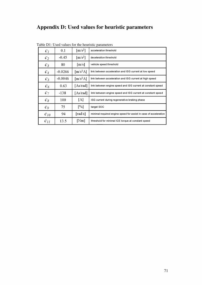
71

Appendix D: Used values for heuristic parameters Table D1: Used values for the heuristic parameters

72

Appendix E: Results of the heuristic strategy on EPA cycles

Figure E1 a) Speed profile of EPA city cycle

b) IBatt(t) from heuristic strategy for EPA city cycle c) Optimal path for IBatt(t) as computed by DP for EPA city cycle

Figure E2 a) Speed profile of EPA highway cycle

b) IBatt(t) from heuristic strategy for EPA highway cycle c) Optimal path for IBatt(t) as computed by DP for EPA highway cycle

73

Appendix F: Results of the analytical strategy on EPA cycles

Figure F1 a) Speed profile of EPA city cycle

b) IBatt(t) from analytical strategy for EPA city cycle c) Optimal path for IBatt(t) as computed by DP for EPA city cycle

Figure F2 a) Speed profile of the EPA highway cycle

b) IBatt(t) from analytical strategy for EPA highway cycle c) Optimal path for IBatt(t) as computed by DP for EPA highway cycle

74

Appendix G: Influence of battery charge acceptance on fuel consumption Table G1: Relation between charge acceptance and FC with analytical strategy

NEDC NEDC EPA CITY EPA HWY Charge acceptance FC FC FC

[A] [l/100 km) [l/100 km) [l/100 km)

25 4.930 5.282 4.379 50 4.910 5.260 4.373 75 4.897 5.244 4.370 100 4.884 5.228 4.367 125 4.873 5.214 4.364 150 4.866 5.202 4.362 175 4.860 5.192 4.360

Table F2: Relation between charge acceptance and FC benefit with analytical strategy

NEDC NEDC EPA CITY EPA HWY charge acceptance benefit benefit benefit

[A] [%] [%] [%]

25 0.59 0.66 0.12 50 0.98 1.06 0.25 75 1.24 1.36 0.32 100 1.50 1.66 0.39 125 1.72 1.92 0.46 150 1.87 2.15 0.50 175 1.98 2.34 0.55