impact of fertilizers and pesticides on india’s

International Journal of Social Science and Economic Research

ISSN: 2455-8834

Volume:06, Issue:09 "September 2021"

www.ijsser.org Copyright © IJSSER 2021, All rights reserved Page 3339

IMPACT OF FERTILIZERS AND PESTICIDES ON INDIA’S

AGRICULTURAL PRODUCTIVITY: A STUDY USING OLS MODEL

Sankalp Rawal

Department of Economics, Aryabhatta College, University of Delhi, New Delhi, India, 110021

DOI: 10.46609/IJSSER.2021.v06i09.018 URL: https://doi.org/10.46609/IJSSER.2021.v06i09.018

ABSTRACT

The significance of the secondary and tertiary sectors in India's GDP is increasing, yet the

primary sector or agriculture, in particular, has always been vital for India's growth. The

agriculture sector depends on critical inputs such as pesticides and fertilizer. This paper seeks to

quantify and analyze the impact of fertilizers and pesticides on India's agricultural yield from

1980 to 2014. A multiple linear regression model using the Ordinary Least Squares (OLS)

method is derived to obtain the required results. The paper also presents additional tests

performed to check for OLS violations and validate the results derived from the model. The

paper's findings suggest that an increase in 1% of the fertilizer consumption by Indian farmers

increases India's mean predicted total agriculture yield by 0.186406%, keeping consumption of

pesticides constant. Likewise, an increase of 1% of the consumption of pesticides by Indian

farmers increases India's mean predicted total agriculture yield by 0.0746664%, keeping

fertilizers constant.

Keywords: Agriculture yield, Farmers, Fertilizer, India, Pesticide, Ordinary Least Squares

1. Introduction

1.1 Why is a study on India’s agriculture sector critical?

The role of the agriculture sector in boosting the Indian Economy can be considered significant

because it was the only sector that clocked positive growth of 3.4% at constant prices in 2020-21.

The agriculture sector continues to be the largest employer of the unskilled and partially skilled

labour force since Independence, employing more than 50% of India’s population. Although

India is the fourth-largest producer of agricultural goods, its agriculture sector, like any other

economy, is highly dependent on fertilizers and pesticides to increase agricultural productivity.

Fertilizers have proven to revolutionize the agriculture sector of many countries experiencing

non-agriculture friendly environments like Qatar and Bahrein and, therefore, can be considered a


ISSN: 2455-8834



critical input to increase crop yield of various food grains commercial crops. The role of

pesticides must also not be underrated. They have been a fundamental part of the agriculture

process by mitigating the losses from weeds, diseases and insect pests that can significantly

impact the volume of harvestable produce. Warren (1998) scrutinized the unforeseen growth in

crop production by using pesticides in the US in the twentieth century. Webster et al. (1999)

claimed that farmers might incur economic losses without the use of pesticides and measured the

remarkable enrichment in crop yield and economic margin that resulted from the use of

pesticides. Since both fertilizers and pesticides are primary inputs in the agriculture process,

carrying an intensive study of how consumption of fertilizers and pesticides by Indian farmers

has affected the total agriculture yield of India becomes a matter of great concern.

Hence, this paper estimates the impact of these two inputs on India’s total crop yield from 1980

to 2014 by implementing an OLS (Ordinary Least Squares) regression model. OLS is widely

used to estimate the parameter of a linear regression model.

2. Material and Method

2.1 Reference to a research paper

This paper derives its base from the research paper written by John W. McArthur and Gordon C.

McCord, which focuses on the role of agriculture inputs, primarily fertilizers including other

inputs, in the growth of the agriculture output of the world. The estimation tool adopted by them

concentrates upon a cross-country panel data set built for developing countries over the period

1961–2001. Their model employs a novel instrumental variable to study the ultimate connection

between alternations in cereal yields and aggregate economic outcomes.

2.2 Reference to an article

Another insightful article written by Md. Wasim Aktar, Dwaipayan Sengupta, and Ashim

Chowdhury provides essential information on the role of pesticides in the agriculture process by

explaining the benefits and shortcomings of its use and comparing its pattern of use in India with

global standards. The article is unique because it highlights various examples where the overuse

of pesticides has negatively impacted agriculture yield.

2.3 About the statistical tool employed

The paper administers multiple linear regression as the primary statistical tool to estimate the

influence of pesticides and fertilizers on India’s agriculture yield. The regression is carried out

using GRETL’s OLS method. OLS is widely used to estimate the unknown parameter of a linear


ISSN: 2455-8834


www.ijsser.org Copyright © IJSSER 2021, All rights reserved 341

regression model as they are considered the best linear unbiased estimators. The objective of the

OLS method is the minimization of the difference between given values and predicted values.

However, the OLS method makes certain assumptions that need comprehension before

performing regression:

1) The regression model is linear in parameter; it may or may not be linear in the variables.

2) The explanatory variable is stochastic and uncorrelated with the error term.

3) Given the value of an explanatory variable, the mean value of the error term is zero.

4) The variance of each error term is constant or homoscedastic.

5) There is no autocorrelation, or two error terms are not correlated.

6) The regression model is correctly specified.

7) Error terms should be normally distributed.

8) There is no multi-collinearity (or perfect collinearity).

9) Number of observations should be more than the number of explanatory variables.

3. Data

3.1 Description of data used

Total agriculture yield (in tonnes per hectare) measures the total yield of major commercial crops

and food grains produced (in tonnes per hectare) by farmers in India annually. The data for total

agriculture yield (dependent variable) is extracted from the official website of the Reserve Bank

of India.

2) Consumption of fertilizers (in tonnes per hectare) measures the total quantity of fertilizers

(Nitrogen + Phosphorous + Potassium) used by Indian farmers annually (in tonnes per hectare)

to increase their agriculture output. The data for consumption of fertilizers (independent

variable) has also been obtained from the Food and Agriculture Organization of the United

Nations.

3) Consumption of pesticides (in tonnes per hectare) measures the total quantity of pesticides

(Technical Grade Materials) used by Indian farmers annually (in tonnes per hectare) in the

agriculture process. The data for the consumption of pesticides (independent variable) has been

obtained from the Food and Agriculture Organization of the United Nations.


ISSN: 2455-8834



3.2 Transforming the original variables

To obtain better results, all three variables have been scaled and transformed into their respective

natural logarithmic forms. Hence, in the OLS model, the variables are interpreted as follows:

LogF = Loge[Consumption of fertilizers(in tonnes per hectare)]

LogP= Loge[Consumption of pesticides(in tonnes per hectare)]

LogAY= Loge[Total agriculture yield(in tonnes per hectare)

4. Graphs and OLS Model

4.1 Graphs

Figure 1: Graph showing the values of LogF from 1980 to 2014

Source: Computed from GRETL


ISSN: 2455-8834



Figure 2: Graph showing the values of LogAY from 1980 to 2014


Figure 3: Graph showing the values of LogP from 1980 to 2014



ISSN: 2455-8834



Figures 1, 2 and 3 portray the logarithm graphs of the variables used in OLS model 1. They

represent relative change rather than an absolute one. The first difference of log for all figures

illustrates the corresponding percentage change in their Y-axis variable.

4.2 OLS Model

The OLS Model 1 quantifies the impact of explanatory variables (LogF and LogP) on LogAY

(dependent variable).

Figure 4: OLS Model 1 showing the impact of LogF and LogP on LogAY

Note: 0.05 or 5% is assumed as the level of significance while building all models and

conducting all tests


From figure 4, we can derive the regression equation as follows:

LogYt= 5.38181 + 0.186406LogX1t + 0.0746664LogX2t + μt


ISSN: 2455-8834



Where,

Yt= Total agriculture yield (in tonnes per hectare) in time period t

X1t = Consumption of fertilizers (in tonnes per hectare) in time period t

X2t= Consumption of pesticides (in tonnes per hectare) in time period t

β1= intercept term= 5.38181

β2= slope coefficient of LogX1t= 0.186406

β3= slope coefficient of LogX2t= 0.0746664

μt= error term

5. OLS Violations

5.1 Multicollinearity

Multicollinearity is the situation of high intercorrelations between independent variables in a

multiple regression model. The high correlation poses a problem because explanatory variables

should not influence each other, leading to skewed results. For verifying whether the OLS Model

1 suffers from multicollinearity, we use two methods in particular.

1) Correlation matrix:

(Null hypothesis) H0: No multicollinearity

(Alternate hypothesis) HA: Multicollinearity is present

Figure 5: Matrix portraying the correlation between LogF and LogP


Figure 5 shows that the explanatory variables are not highly correlated as the correlation between

them is only -0.42 approximately. Therefore, the problem of multicollinearity must not persist in


ISSN: 2455-8834



the model. However, we also check for multicollinearity through the method of variance

inflation factors.

2) Variance inflation factors(VIF):

Figure 6: Testing for multicollinearity in OLS Model 1 using VIF


Figure 6 shows that the VIF values of the variables in question are less than 10. Both the

explanatory variables have a VIF value of 1.221. Hence, we can rightfully claim that the model

does not have a collinearity problem.

5.2 Heteroscedasticity

OLS assumes that the variance of the error term is constant (Homoscedasticity).The model

suffers from heteroscedasticity if the error terms do not have constant variance. The existence of

heteroscedasticity is a major concern in applying regression analysis, including the analysis of

variance, as it can invalidate statistical tests of significance.

White’s test:

H0: Heteroscedasticity is not present (Homoscedasticity)


ISSN: 2455-8834



Ha: Heteroscedasticity is present

Figure 7: Testing for heteroscedasticity in OLS Model 1 using White’s test


Since the p-value in figure 7 is greater than the level of significance (0.353663 > 0.05) therefore

we have insufficient evidence to reject the null hypothesis (H0). That means heteroscedasticity is

not present in the model.

5.3 Autocorrelation

Autocorrelation in the model exists when the error terms are correlated with each other, which

leads to skewed and misleading results. Breusch-Godfrey test and Durbin Watson test are

executed to check for autocorrelation in the model.

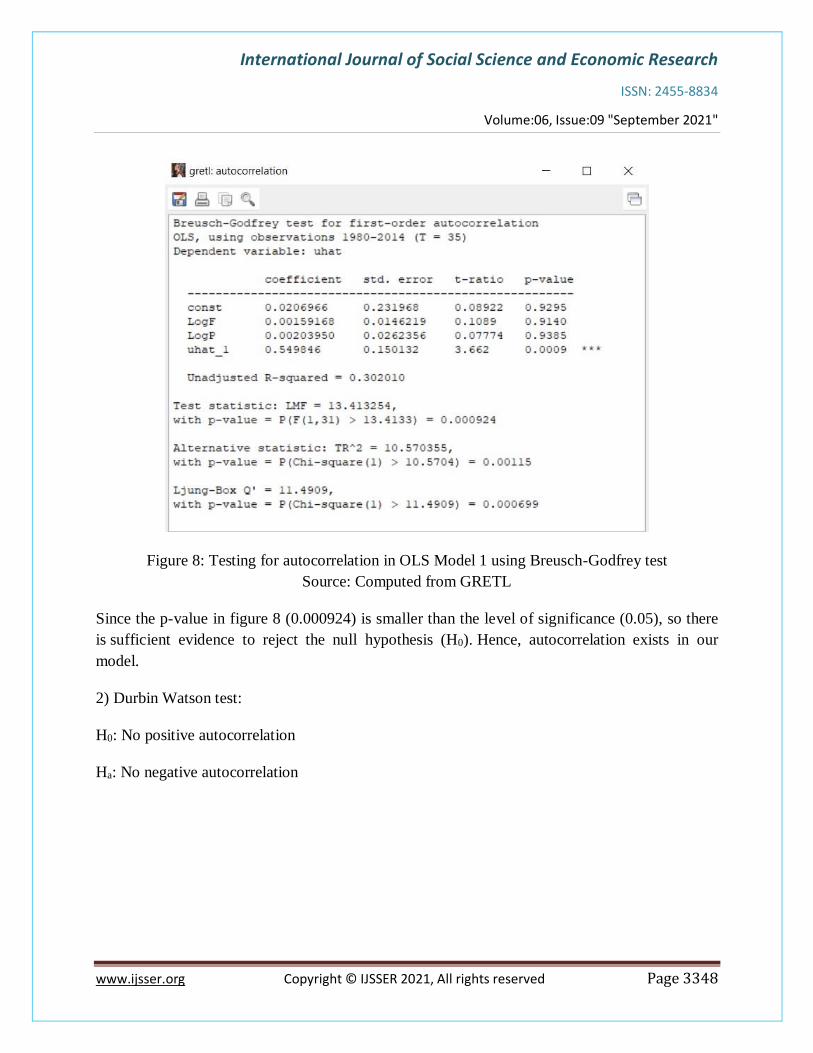
1) Breusch-Godfrey test:

H0: Autocorrelation is not present

Ha: Autocorrelation is present


ISSN: 2455-8834



Figure 8: Testing for autocorrelation in OLS Model 1 using Breusch-Godfrey test


Since the p-value in figure 8 (0.000924) is smaller than the level of significance (0.05), so there

is sufficient evidence to reject the null hypothesis (H0). Hence, autocorrelation exists in our

model.

2) Durbin Watson test:

H0: No positive autocorrelation

Ha: No negative autocorrelation


ISSN: 2455-8834



Figure 9: Testing for autocorrelation in OLS Model 1 using Durbin Watson test


k’=2 (Calculated)

dL=1.303 (Calculated)

dU=1.584 (Calculated)

Since the Durbin Watson statistic (0.877736) in figure 9 is smaller than dL, we reject the null

hypothesis (H0). Hence, there is no positive autocorrelation in the model, but

negative autocorrelation exists.

5.4 Remedial measure of autocorrelation

In order to remove autocorrelation from OLS Model 1, PraisWinsten’s approach is used as a

remedy.

We regress,

LogAYt*= β1

*+ β2*(LogFt

*) + β3*(LogPt

*) + ȗt

Where,

LogAYt*= LogAYt- p̂LogAYt-1

LogFt*= LogFt- p̂LogFt-1

LogPt*= LogPt- p̂LogPt-1


ISSN: 2455-8834



and,

LogAY1* = LogAY1(1- p̂2)0.5

LogF1*= LogF1(1- p̂2)0.5

LogP1*= LogP1(1- p̂2)0.5

p̂= 0.549309(obtained from OLS Model 1), p̂2= 0.3017403

Now, running a regression model on the starred variables using OLS on GRETL and checking

for autocorrelation, the following results are obtained:

Figure 10: Testing for autocorrelation after executing Prais Winston’s remedy


Since the test statistic p-value (0.0601) in figure 10 is greater than the level of significance (0.05)

so there is insufficient evidence to reject the null hypothesis (H0). Hence, the model does not

have autocorrelation anymore. Moreover, the Durbin Watson statistic of the new model is 1.311,

which is greater than dL,so there is no autocorrelation in the model now.


ISSN: 2455-8834



5.5 Specification biasedness

Ramsey’s RESET test (squares only):

H0: Specification is adequate

Ha: Specification is inadequate

Figure 11: Testing for specification biasedness in OLS Model 1 using RESET test


Since the p-value (0.894) in figure 11 is greater than the level of significance (0.05), so there is

insufficient evidence to reject the null hypothesis (H0). Hence, the specification is adequate.

6. Additional Tests

6.1 Joint Significance test

H0: β2= β3=0


ISSN: 2455-8834



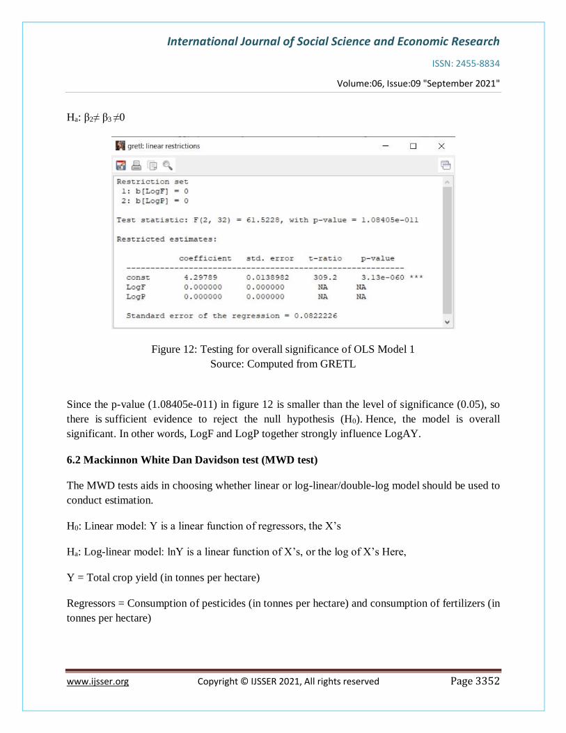
Ha: β2≠ β3 ≠0

Figure 12: Testing for overall significance of OLS Model 1


Since the p-value (1.08405e-011) in figure 12 is smaller than the level of significance (0.05), so

there is sufficient evidence to reject the null hypothesis (H0). Hence, the model is overall

significant. In other words, LogF and LogP together strongly influence LogAY.

6.2 Mackinnon White Dan Davidson test (MWD test)

The MWD tests aids in choosing whether linear or log-linear/double-log model should be used to

conduct estimation.

H0: Linear model: Y is a linear function of regressors, the X’s

Ha: Log-linear model: lnY is a linear function of X’s, or the log of X’s Here,

Y = Total crop yield (in tonnes per hectare)

Regressors = Consumption of pesticides (in tonnes per hectare) and consumption of fertilizers (in

tonnes per hectare)


ISSN: 2455-8834



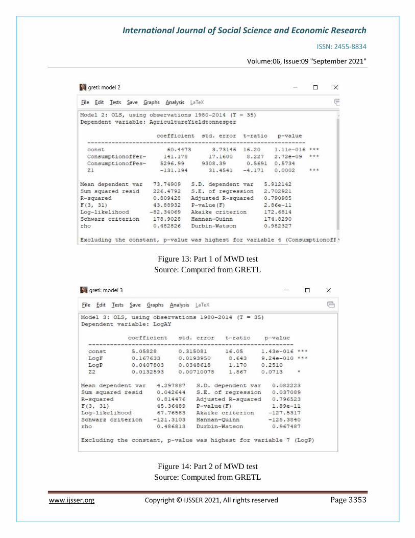
Figure 13: Part 1 of MWD test


Figure 14: Part 2 of MWD test



ISSN: 2455-8834



Since the p-value of Z1 in figure 13, that is, 0.0002 is lower than the significance level (0.05),

we have sufficient evident to reject the null hypothesis (H0). Moreover the p-value of Z2 in figure

14, that is, 0.0713 is greater than the significance level (0.05). Hence,we have insufficient

evidence to reject Ha. Hence, we can say that Z2 is not statistically significant. It implies that the

log-linear model or double-log model fits correct.

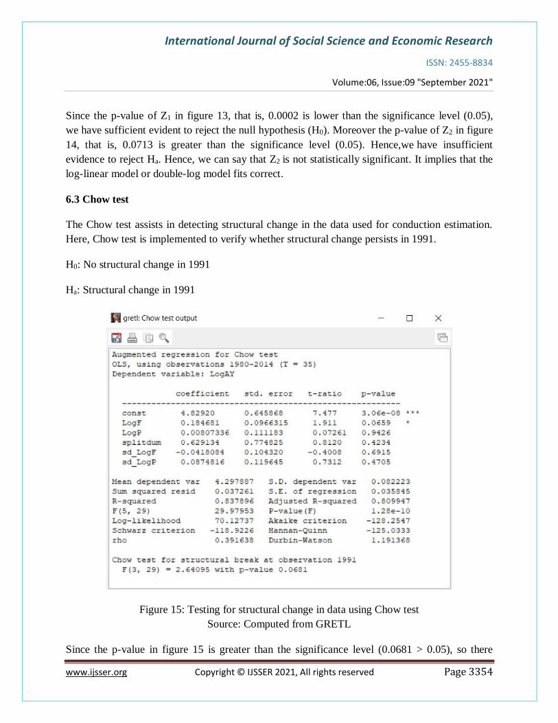
6.3 Chow test

The Chow test assists in detecting structural change in the data used for conduction estimation.

Here, Chow test is implemented to verify whether structural change persists in 1991.

H0: No structural change in 1991

Ha: Structural change in 1991

Figure 15: Testing for structural change in data using Chow test


Since the p-value in figure 15 is greater than the significance level (0.0681 > 0.05), so there


ISSN: 2455-8834



is insufficient evidence to reject the null hypothesis (H0). It implies that there is no

structural change in 1991.

6.4 Normality of residual

If the error terms are not normally distributed,then the forecasts, confidence intervals yielded by

a regression model may not be BLUE (BEST LINEAR UNBIASED ESTIMATOR).

H0: Errors are normally distributed

Ha: Errors are not normally distributed

Figure 16: Testing for normal distribution of errors in OLS Model 1


Test statistic: Chi-square (2) = 0.130

With p-value = 0.9372


ISSN: 2455-8834



Since the p-value (0.9372) in figure 16 is more than the significance level (0.05) therefore there

is insufficient evidence to reject the null hypothesis (H0). It implies that errors are normally

distributed.

7. Results

7.1 Interpretation of OLS Model 1

The OLS Model 1 indicates that an increase in 1% of the consumption of fertilizer by Indian

farmers increases India's mean predicted total agriculture yield by 0.186406%, keeping

consumption of pesticides constant. In other words, β2 measures the partial elasticity of Yt with

respect to X1t, holding the influence of X2t constant. Hence, total agriculture yield is partially

inelastic with respect to the consumption of fertilizers. An increase of 1% of the consumption of

pesticides by Indian farmers increases India's mean predicted total agriculture yield by

0.0746664%, keeping consumption of fertilizers constant. In other words, β3 measures the partial

elasticity of Yt with respect to X2t, holding the influence of X1t constant. Hence, total agriculture

yield is partially inelastic with respect to the consumption of pesticides. The mean predicted

LogAY is 5.5818 when LogF and LogP are fixed at zero. The t ratios for all the explanatory

variables are significant. Moreover, the signs of coefficients satisfy economic theory. R-squared

of 0.793609 signifies that LogF and LogP explain 79.3609% of the variation in LogAY.

7.2 Summarising the results of all tests

As far as the validity of the results derived from the model is concerned, the model is overall

significant. OLS violations such as specification biasedness, heteroscedasticity and collinearity

are not present in the model. The residuals are normally distributed in the model, implying that

the classical linear regression model assumptions hold. Although autocorrelation persists, the

problem is resolved by applying Prais Winston's approach. Finally, the chow test confirms that

there is no structural change in 1991.

8. Discussion

As stated before, the objective of the study was to determine the impact of consumption of

fertilizers (in tonnes per hectare) and consumption of pesticides (in tonnes per hectare) on total

crop yield (in tonnes per hectare). The OLS model results agree with the empirical evidence,

which suggests that fertilizers and pesticides are crucial for enhancing agriculture yield.

However, it is essential to realize that factors outside the scope of this study, such as labour,

capital employed, rainfall and other climatic factors, also contribute towards raising the

agriculture yield, as economic theory suggests. Therefore, drawing keen attention to the adequate


ISSN: 2455-8834



supply of these inputs is also critical for meeting production goals.

9. Acknowledgement

I would like to express my deep and sincere gratitude to my professors at the Economics Faculty

of Aryabhatta College for granting me the opportunity to research on the chosen topic and

providing invaluable guidance throughout this research. I acknowledge them for their valuable

support, cooperation, and patience, which helped me successfully complete this paper.

References

1)McArthur and McCord, Journal of Development Economics, Volume 127, “Fertilizing growth:

Agricultural inputs and their effects in economic development”, Pages-133 to 152, Published-

2017, https://www.sciencedirect.com/science/article/pii/S0304387817300172

2) Aktar, Sengupta and Chowdhury, National Center for Biotechnology Information, “Impact of

pesticides use in agriculture: their benefits and hazards, Published- 2009,

https://www.ncbi.nlm.nih.gov/pmc/articles/PMC2984095/, (24/05/2021)

3) Reserve Bank of India, Database on Indian economy, Data for agriculture yield from 1980 to

2014; https://dbie.rbi.org.in/DBIE/dbie.rbi?site=statistics, (20/05/2021)

4) Food and Agriculture Organization of the United Nations, Data for fertilizer and pesticide use

from 1980 to 2014; http://www.fao.org/faostat/en/#data, (20/05/2021)

https://www.sciencedirect.com/science/article/pii/S0304387817300172

https://www.ncbi.nlm.nih.gov/pmc/articles/PMC2984095/

https://dbie.rbi.org.in/DBIE/dbie.rbi?site=statistics

http://www.fao.org/faostat/en/#data

impact of fertilizers and pesticides on india’s

Documents