impact of agricultural profitability, productivity and

University of Arkansas, FayettevilleScholarWorks@UARK

Theses and Dissertations

8-2011

Impact of Agricultural Profitability, Productivityand Interest Rate on Farmland Value for SelectedU.S. and Slovak StatesMaria MajerhoferovaUniversity of Arkansas, Fayetteville

Follow this and additional works at: http://scholarworks.uark.edu/etd

Part of the Agricultural Economics Commons, Finance Commons, and the IndustrialOrganization Commons

This Thesis is brought to you for free and open access by ScholarWorks@UARK. It has been accepted for inclusion in Theses and Dissertations by anauthorized administrator of ScholarWorks@UARK. For more information, please contact [email protected], [email protected].

Recommended CitationMajerhoferova, Maria, "Impact of Agricultural Profitability, Productivity and Interest Rate on Farmland Value for Selected U.S. andSlovak States" (2011). Theses and Dissertations. 123.http://scholarworks.uark.edu/etd/123

http://scholarworks.uark.edu?utm_source=scholarworks.uark.edu%2Fetd%2F123&utm_medium=PDF&utm_campaign=PDFCoverPages

http://scholarworks.uark.edu/etd?utm_source=scholarworks.uark.edu%2Fetd%2F123&utm_medium=PDF&utm_campaign=PDFCoverPages

http://scholarworks.uark.edu/etd?utm_source=scholarworks.uark.edu%2Fetd%2F123&utm_medium=PDF&utm_campaign=PDFCoverPages

http://network.bepress.com/hgg/discipline/1225?utm_source=scholarworks.uark.edu%2Fetd%2F123&utm_medium=PDF&utm_campaign=PDFCoverPages




http://scholarworks.uark.edu/etd/123?utm_source=scholarworks.uark.edu%2Fetd%2F123&utm_medium=PDF&utm_campaign=PDFCoverPages

mailto:[email protected],%[email protected]

IMPACT OF AGRICULTURAL PROFITABILITY, PRODUCTIVITY AND

INTEREST RATE ON FARMLAND VALUE FOR SELECTED U.S. AND SLOVAK

STATES

IMPACT OF AGRICULTURAL PROFITABILITY, PRODUCTIVITY AND

INTEREST RATE ON FARMLAND VALUE FOR SELECTED U.S. AND SLOVAK

STATES

A thesis submitted in partial fulfillment

of the requirements for the degree of

Master of Science in Agricultural Economics

By

Maria Majerhoferova

Slovak University of Agriculture in Nitra

Master of Science in Rural Development, 2009

August 2011

University of Arkansas

ABSTRACT

This thesis examines agricultural factors which may have impact on agricultural

land values. Based on theory, three primary factors are considered to have an impact on

land value: agricultural productivity, agricultural profitability and interest rate. The study

is of two countries: the US, where data are from 16 states and Slovakia with 6 states. The

ten-year period from 2000 until 2009 is used in the analysis. A capitalization model is

used to estimate the relationship between agricultural productivity, profitability and

interest rate and land value. Three types of agricultural land are used: cropland and its

value in relationship with crops, grassland and its value in relationship with animals and

agricultural land and its value in relationship with animals and crops. The estimated

results indicate profitability, when proxied by revenue and expenses, and interest rate as

significant variables in all US models. Profitability proxied by profit is an insignificant

variable. Productivity is significant only in the US crop models. Results from the Slovak

models indicate the interest rate as the only significant variable. Unfortunately, the

collection of land value data in Slovakia is not very functional, which can be seen in huge

differences in values between years and very high values in some states, such that the

validity of the data is questionable.

This thesis is approved for recommendation

to the Graduate Council.

Thesis Director:

____________________________________

Dr. Bruce L. Ahrendsen

Thesis Committee:

___________________________________

Dr. Harold L. Goodwin, Jr.

__________________________________

Dr. Anna Bandlerova

THESIS DUPLICATION RELEASE

I hereby authorize the University of Arkansas Libraries to duplicate this thesis

when needed for research and/or scholarship.

Agreed ________________________________

Maria Majerhoferova

Refused ________________________________

Maria Majerhoferova

v

ACKNOWLEDGEMENTS

A special thanks to Dr. Bruce L. Ahrendsen who offered me invaluable assistance,

advice and guidance, invested his time in my research and supported me in completing

my goal.

It is a pleasure to thank prof. JUDr. Anna Bandlerova, PhD., for her valuable input,

suggestions, helpful comments and friendly support.

I would like to thank to Dr. Harold L. Goodwin Jr. for his ideas and enthusiasm

which he has provided.

I would like to thank Dr. Bruce L. Dixon for his help with LIMDEP software and

econometric issues. Thanks to Diana Danforth for her help with SAS software.

I would like to thank the Department of Agricultural Economics and Agribusiness

for new experiences and fellowship.

vi

DEDICATIONS

I dedicate this thesis to my family. Thank you for your love, patience, moral and

financial support.

vii

TABLE OF CONTENTS

I. INTRODUCTION 1

I.1. Purpose of Study and Hypothesis 1

I.2. Forthcoming Chapters 2

II. REVIEW OF PREVIOUS STUDIES 4

2.1. History of Farmland Price Development 4

2.2 Agricultural Land Values in U.S. 5

2.3 Factors Determining Land Value 9

2.4 Land Ownership and Covers in U.S. 11

2.5 Land Quality 13

2.6 Land-use Regulations 14

2.7 Urbanization and Land Value 15

2.8 Land Policies 16

2.9 The Impact of Government Payments on Farmland Values 17

2.10 Commodity Policies 18

2.11 Land Value Models 19

2.11 Land Development in Slovakia until 1999 21

2.12 Current Situation 23

2.13 Owners of Land 25

2.14 Market and Administrative Prices 26

2.15 Functionality of Land Records and Information 33

III. DATA AND METHODS 34

3.1 Data Source 34

3.2 Variables and Variable Specifications 36

3.2.1 Measure of Profitability 36

3.2.2 Productivity Index 40

3.2.3 Deflation of Values and Interest Rate 41

3.3 Content of data 42

3.4 Methodology 45

viii

3.4.1 Capitalization Model 47

IV. EMPRICAL RESULTS 49

4.1 The Economic Software and Tests for Violations 49

4.2 U.S. Total Model with Profitability Proxied by Profit 51

4.3 U.S. Crop Model with Profitability Proxied by Profit 52

4.4 U.S. Animal Model with Profitability Proxied by Profit 53

4.5 U.S. Total Model with Profitability Proxied by Revenues and Expenses 55

4.6 U.S. Crop Model with Profitability Proxied by Revenues and Expenses 56

4.6 U.S. Animal Model with Profitability Proxied by Revenues and Expenses 58

4.7 SK Total Model with Profitability Proxied by Profit 61

4.8 SK Crop Model with Profitability Proxied by Profit 63

4.9 SK Animal Model with Profitability Proxied by Profit 64

4.10 SK Total Model with Profitability Proxied by Revenues and Expenses 65

4.11 SK Crop Model with Profitability Proxied by Revenues and Expenses 66

4.12 SK Animal Model with Profitability Proxied by Revenues and Expenses 67

V. SUMMARY AND CONCLUSION 71

VI. BIBLIOGRAPHY 75

VII. Appendices 80

Appendix A 80

Appendix B 96

ix

LIST OF TABLES

Table 2.1 The Impact of an Increase in Certain Variables on Land Value 11

Table 2.2 Market and Administrative Prices for Selected Slovak States in 2009 29

Table 2.3 Price and Rent for Agricultural Land in Slovakia 31

Table 3.1 Summary Statistics for U.S. Data Used to Estimate Land Price Models 42

Table 3.2 Summary Statistics for Slovak Data Used to Estimate Land Price Models 43

Table 3.3 List of variables 44

Table 4.1 U.S. Total Model 52

Table 4.2 U.S. Crop Model 53

Table 4.3 U.S. Animal Model 54

Table 4.4 U.S. Total Model 56

Table 4.5 U.S. Crop Model 57

Table 4.6 U.S. Animal Model 59

Table 4.7 Summary of U.S. models 60

Table 4.8 SK Total Table 63

Table 4.9 SK Crop Model 64

Table 4.10 SK Animal Model 65

Table 4.11 SK Total Model 66

Table 4.12 SK Crop Model 67

Table 4.13 SK animal model 68

Table 4.14 Summary of results for SK models 69

x

LIST OF FIGURES

Figure 2.1 Average U.S. Farm Real Estate Value, Nominal and Real 6

Figure 2.2 U.S. Agricultural Land Values 7

Figure 2.3 Farm Real Estate Value in U.S. 8

Figure 2.4 Cropland Value in U.S. 9

Figure 2.5 Federal Land as a Percentage of Total State Land Area 12

Figure 2.6 Total Surface Area by Land Cover/Use in 2007 13

Figure 2.7 Price of land 27

Figure 2.8 Administrative and Market Price of Land in Chosen States in Slovakia 30

Figure 2.9 Average Market Price of Agricultural Land in Chosen States in Slovakia 32

Figure 2.10 Price of Agricultural Land in Different Countries of the EU 33

Figure 3.1 The Sixteen U.S. States 34

Figure 3.2 The Six Slovakia States 35

1

I. INTRODUCTION

1.1 Purpose of Study and Hypothesis

Land is an important and valuable resource for human life. Its contribution is not

only in terms of urbanization and environment but also in agriculture.

Agricultural land is strongly connected to agricultural production, and we can say

that is its main factor. Consequently, agricultural production has an impact on the value

of agricultural land. There is a very strong relationship between them.

In this study the focus is on agricultural factors which may have an impact on

agricultural land value. Agricultural land values in two countries are compared: the U.S.

where data from 16 states are used and Slovakia with 6 states. Based on theory, three

primary factors are considered to have an impact on land value: agricultural profitability,

agricultural productivity and interest rate. Three types of agricultural land are used:

cropland and its value in relationship with crops, grassland and its value in relationship

with animals and agricultural land and its value in relationship with animals and crops.

The theoretical model used is the capitalization model, which relates land values to

agricultural profitability, productivity and interest rate. To measure profitability, several

proxies are used: profit, revenue and expenses, cash rent, or output and input price

indices. For productivity, yield is used for crops or weight gain is used for animal

production. The ten-year period of 2000 through 2009 is used in the analysis.

The objective is to estimate the relationship of land value with agricultural

profitability, productivity and interest rate. This includes testing three hypotheses.

The first null hypothesis is agricultural land (cropland or pasture land) value is not

related to agricultural (crop or animal) profitability. The second null hypothesis is

2

agricultural land (cropland or pasture land) value is not related to agricultural

productivity (crop or animal). Finally, the third null hypothesis is agricultural land is not

related to interest rate.

Based on the theory and study of previous literature concerning this topic, the

corresponding alternative hypotheses are agricultural land (cropland and pasture land)

value is: 1) positively related to agricultural (crop or animal) profitability, 2) positively

related to agricultural (crop or animal) productivity, and 3) negatively related to interest

rate.

1.2 Forthcoming Chapters

In the first part of the study, the focus is on all possible factors having an

influence on U.S. land value, some of them with very strong and some with slightly less

impact. Included in this part are descriptions of the history of farmland price

development, private and federal land ownership in the U.S., major use of land, urban

development of the land, ambition of the U.S. government to protect highly productive

agricultural land through conservation programs, and the impact of commodity policies.

While the U.S. land market is developed and land values have experienced an

increasing trend within the study period, the land market in Slovakia is still developing

after the period of centrally planned economy where land was managed mainly by the

state. Nowadays, the Slovak government has had to deal with situations like unknown

owners of land or disinterest by people to cultivate the land. One of the problems is also

collecting the data concerning land value, profitability and productivity. Statistical offices

and networks, which collect data, are not really functional. This can be seen in the land

3

value data, where the percentage change in land value from one year to the next within

the study period is highly variable.

In the second part of the study, the methods I used to collect and compute data

and to estimate missing data are described. The data are mostly taken from official

government websites like the U.S. Department of Agriculture’s (USDA) National

Agricultural Statistics Service (NASS) and Economic Research Service (ERS) in the U.S.

and the Statistical Office of the Slovak Republic and regional statistical offices in

Slovakia.

Also in the second part, the methodology for modeling the relationship between

the dependent and independent variables is described. Also possible violations in the

model’s underlying assumptions, such the presence of autocorrelation, heteroskedasticity

and multicollinearity and ways to deal with them are discussed.

The next part of the study is about empirical results. In the case of the U.S., most

of the results are in accordance with the expectations, especially for agricultural revenue,

where there was a strong relationship with land value. In contrast, profit and productivity

did not show a consistently significant relationship with land value. In the case of

Slovakia the results are not satisfying. The main reason may be a result of possibly

unreliable data collected by the statistical offices.

4

II. REVIEW OF PREVIOUS STUDIES

2.1. History of Farmland Price Development

During the period of “the Golden Age’’ of American agriculture, from 1910 till

1914, the value of farmland almost doubled as a result of the increasing trend in the farm

product price. During the next period, from 1921 till 1933, the agriculture sector faced

problems which caused a fall in farm product prices and also a decrease in farmland

prices. The farmland value always followed the farm product price (Cochrane, 2003).

During 1963-1982 the price of land almost doubled. Alston (1986) describes two

main competing reasons of this increase. The first one was connected with the real

growth of land rental income and the second one was connected with inflation and tax

laws. According to his research, inflation has a very small influence on land price while

the main factor in increasing the land price is the real growth of rental income.

Just and Miranowski (1993) see different variables affect the rise and decline in

land value. They describe the role of inflation and the opportunity cost of capital as the

most important variables. During the 1970s, there was an increase in the inflation rate,

and this effect explained 25% of the predicted price increase. The opportunity rate of

return on capital fell and that had an impact on the attractiveness of land as an investment

which caused an increase in the land price. Another variable with a high impact on land

value is returns to farming which explained 30% of the predicted land price change. The

impact of government payments on capitalized land values is around 25%, but

government payments do not have a significant impact on year-to-year changes.

Adoption of new farm technology, a free land market and a fixed supply of land

were typical for the period 1933 till 2003. Farmers were interested in increasing their

5

asset portfolio by buying more land. Price of land together with production costs were

increasing. Supply of products also had an increasing trend and prices of products were

decreasing. The profit of farmers was really low. Government decided to help them by

supporting output prices. The result of this aid had an impact of increasing the price of

land (Cochrane, 2003).

2.2 Agricultural Land Values in U.S.

From 1970 to 1981, real farm real estate values increased 94%, which was the

result of high returns and federal policies (Figure 2.1). This period was following by a

decline in farm real estate values, which was in response to increased interest rates that

was a result of monetary policy to lower inflation. This period of declining farm real

estate values coincided with a period that is often referred to as the farm financial crisis

during the 1980s. For 1987-1993, real land values were relatively stagnant before starting

a slow increase until 2004. A sharp increase followed from 2005 to 2008. Then real farm

real estate values decreased slightly because of world economic crises (USDA, ERS,

2011).

6

Figure 2.1 Average U.S. Farm Real Estate Value, Nominal and Real (Inflation

Adjusted), 1970-2000

Source: USDA, ERS, Agricultural Land Values, 2011

Usually cropland values are two-three times higher than pastureland values

(Figure 2.2). There is a continuous increase in agricultural land values from 1997 through

2008.

7

Figure 2.2 U.S. Agricultural Land Values

Source: USDA, NASS, 2010

Figure 2.3 shows the Farm Real Estate Value, which is a measurement of the

value of all land and buildings on farms, by each state and the change in value between

the years 2009 and 2010. The highest values, with averages of more than $10,000 per

acre, are in Rhode Island, New Jersey and Connecticut and the smallest values, with

averages less than $800 per acre, are in Wyoming, New Mexico and Montana. In general,

states with the highest values are in the Northeast region of the US with an average of

$4,690 per acre in 2010. States with the lowest values are in the Mountain region with an

average of $911 per acre. The region which is closest to the U.S. average of $2,140 per

acre is the Delta region with an average value of $2,230 per acre (USDA, NASS, 2010).

0

500

1000

1500

2000

2500

3000

19

97

19

98

19

99

20

00

20

01

20

02

20

03

20

04

20

05

20

06

20

07

20

08

20

09

20

10

Do

llars

pe

r ac

re

Year

Agricultural Land Values

AG LAND, CROPLAND

AG LAND, INCL BUILDINGS

AG LAND, PASTURELAND

8

Figure 2.3 Farm Real Estate Value in U.S.


Figure 2.4 shows 2010 cropland values by each U.S. state. New Jersey is the only

state with an average cropland value more than $10,000 per acre. The Northeast region

again has the highest average cropland value at $5,220 per acre, which is more than the

average farm real estate value. Montana has the lowest cropland value at less than $800

per acre. However, the region with the lowest average value is not in the region where

Montana is located, but it is in the Northern Plains (USDA, NASS, 2010).

9

Figure 2.4 Cropland Value in U.S.


2.3 Factors Determining Land Value

Earlier studies already determined many different variables and factors which

could have a possible impact on increasing or decreasing land value, for instance:

expansion pressure, net returns, capitalized government payments, market (operating)

returns, farm enlargement, number of transfers, capitalized rent, etc. All of these factors

can influence the land price in different ways and different intensity.

According to Weerahewa et al. (2008) “Land values are based on discounted

expected future returns to land, which is composed of revenue from production and

subsidies.” They were examining the relationship of farmland value with income from

10

the market and government payments for chosen provinces of Canada. He found that

there is no connection between earning per acre and farmland value. Also, even though

there was an increase in farmland values during 2007, the cash flow generated from

farmland did not change so much. They found that any impact of government payments

depends on including or excluding time trend in model. If a time trend is included in the

model, government payments show no significance on land values. If a time trend is

omitted, government payments are significant. They also found that if there is a decrease

in the interest rate, land values tend to increase.

Schmitz and Just (2003) describe farm income as one of the factors having an

impact on land value. They found that between 1910 and 1950 the relationship between

land value and farm income was positive, but during years 1960-1970s the relationship

was negative. They concluded that farm income is not the only and not the strongest

factor affecting land value, and using farm income as the only factor to describe land

value is not recommended. In contrast, they describe inflation as one of the major factors

increasing land value. They also found that the available cash for purchasing land also

has a positive impact on raising land value. Cash availability can be influenced by many

other factors like farmland collateral value, net farm income, and anticipated appreciation

of land value for nonfarm uses.

Moss (1997) examines the importance of different variables in explaining the

variation in land values. He finds that inflation explains most of the differences in land

values, and its relative explanation is around 80% in almost all U.S. regions. Agricultural

returns have explanatory power in the regions which rely on government payments,

which are part of the net farm income.

11

Table 2.1 The Impact of an Increase in Certain Variables on Land Value

Variable Change in land value

Population density Increase

Real Interest Rate Decrease

Government Payment Increase

Net Farm Income Increase

Cash Rent Increase

Risk of income Decrease

Tenure level of counties Ambiguous

Productivity Increase

Size of farm Decrease

Returns to farming Increase

Inflation Increase

Interest rate Decrease

Source: Weerahewa, et al. (2008); Katchova, Sherrick and Barry (2002)

2.4 Land Ownership and Usage in U.S.

The land area of the U.S. is 2.3 billion acres. Land can be divided into two types

of ownership, federally (public) owned lands and privately (nonfederal) owned lands.

The impact of ownership on land is very high in economic, social, and ecological terms.

Public lands are mostly used to bring public good while private lands serve to increase

market return (Ahearn and Alig, 2005a).

12

Most of the federal land is concentrated in the western United States (Figure 2.5).

In 2004, almost 28% of the whole U.S. land is considered to be owned by the federal

government (Jacobs, 2008). This land is managed by the Bureau of Land Management,

the Forest Service, the Fish and Wildlife Service, the National Park Service, and several

others. Nevada has the highest percentage of federally owned land (almost 85%),

followed by Alaska with 61% and Utah with 57%. Connecticut has the lowest percentage

of federally owned land with 0.4%, followed by Rhode Island with 0.4% and Iowa with

0.8%. Privately owned land is mostly concentrated in the East and the West, and in 1997,

it covered about half of the land base, including 406 million acres of rangeland, 377

million of cropland, 120 million acres of pastureland, and 33 million acres of other

agricultural land (Ahearn and Alig, 2005a).

Figure 2.5 Federal Land as a Percentage of Total State Land Area

Source: Jacobs, 2008

13

Rural land covers 1,373,658,800 acres, which is 70.9% of the entire land surface

area (Figure 2.6). Of rural land, cropland covers 357,023,500 acres, rangeland covers

409,119,400 acres, forest land covers 406,410,400 acres, pastureland covers 118,615,700

acres and CRP (the Conservation Reserve Program) covers 32,850,200 acres (Farmland

Information Center, 2007).

Figure 2.6 Total Surface Area by Land Cover/Use in 2007

Source: Farmland Information Center, 2007

2.5 Land Quality

To create new policies, policymakers cannot focus just on quantity of land but

also on quality. Their main attention is focused mostly on when quality, productive land

is converted for another use. During the measurement of land quality it is necessary to

pay attention to the particular use or goal of the land. “Soil quality is often used as a

proxy for suitability for agricultural use.‟‟ (Ahearn and Alig, 2005a).

14

In general, there are eight land classes (Ahearn and Alig, 2005a). The main

indicators of suitability are erosion risk, wetness, and shallowness. When land has the

best combination of physical and chemical attributes, it is considered as prime farmland,

which is the most appropriate class for crop production. The amount of prime farmland

has decreased through time. In 1982, it was 342 million acres, but by 1997 it had fallen

by about ten million acres.

2.6 Land-use Regulations

Wu and Bell (2005) describes the impact of regulations on land use. The

difference between the local and federal government is that the local government focuses

mostly on land use control, and the federal government controls changes in the land use

conversion. Government can be involved in land regulations in different ways, for

example through the conservation program for agricultural and forestry land, the

promotion of industrial and commercial investments, and support for compact

development by creating country comprehensive plans, urban growth boundaries,

housing caps, and agricultural, forestry, and rural residential zoning. The effectiveness of

these regulations may vary. Previous studies found that traditional regulations such as

zoning are not as effective as fiscal policies and price regulations. The only way how

zoning could increase land value is “that residential land values rise as the proportion of

the block that is in residential use increases.‟‟ However, zoning in general does not

increase land values. Other studies have tried to observe the impact of the purchase or

exchange of development rights, but unfortunately, it is very difficult to isolate a specific

program to see its influence.

15

Most of the studies are focused on urbanization sprawl, and they evaluate its

impact very negatively. Urbanization sprawl results in reducing wildlife habitat, poorer

water quality but also in increasing obesity. However, some authors say that urbanization

sprawl is “a result of consumer choices‟‟ (Wu and Bell, 2005).

2.7 Urbanization and Land Value

“Continued in destruction of cropland is wanton squandering of an irreplaceable

resource that invites tragedy not only nationally, but on a global scale.‟‟

Bergland (The U.S. Secretary of Agriculture), retrieved from Plantinga, Lubowski and

Stavins, 2002.

Plantinga, Lubowski and Stavins (2002) focus on the impact of urbanization on

agricultural land. Decreases in agricultural land as the result of urbanization could cause

problems with production of food, which could also have a negative influence on national

security. They found that future development rents in areas close to urban center are

much higher than agricultural land values. The U.S. government would have to apply

strong policies to restrict the purchase of land for development purposes and to keep the

land under cultivation. They also found that there is an impact of unpredictable future

development rents on the farmland value.

In 1996, the U.S. government ratified the Federal Agriculture Improvement and

the Reform Act and the Soil Conservation Service was re-established as the Natural

Resource Conservation Service (NRCS). The NRCS has many programs and activities

focused on protection of land and soil, like preservation, retiring and working lands

programs. One of the easement programs of the NRCS is the Farm and Ranch Land

16

Protection Program (FRPP). The main role of this program is to maintain productive farm

and ranch land for agriculture production by supporting the purchase of development

rights from owners of agricultural land (USDA, NRCS, 2010).

The FRPP aims to avoid transformation of agricultural land to non-agricultural

land. Farmers can make a choice to continue with agricultural development or start urban

development. They can sell their development rights and keep their land for agricultural

uses. The FRPP was also part of the 2002 Farm Bill and was continued by the 2008 Farm

Bill where direct payments are even higher than they were in the 2002 Farm Bill (The

Environmental Defend Fund, 2006).

The U.S. government is using two different policies to prevent the loss of land to

urbanization: conservation programs and direct government subsidies to farmers.

Receivers of direct payments are mostly farm operators of the land. These government

payments are capitalized into the value of the land. The main impact of the government

payment on land value is to increase farmland value (Ahearn and Alig, 2005b).

2.8 Land Policies

The U.S. government uses many factors to influence private land use. Some of the

most used ones are land-use taxes, subsidies, easement, transfer of development rights

and different regulations. The government also creates many public policies, which have

different aims and an additional impact on land use. The main role of today’s U.S. land

policy is to ensure land use in parallel with social, economic and environmental needs

(Ahearn and Alig, 2005b).

17

In terms of the land policy, the USDA is responsible for:

Retaining an adequate size of land for cultivation and to assure high quality food

at reasonable production costs and in sufficient supply.

Protecting the most profitable lands and forests from urbanization, but at the same

time helping landlords with development so they can meet their needs.

Looking after quality of environment (Ahearn and Alig, 2005b).

To avoid the loss of profitable agricultural land and forests due to “urban

sprawl’’, the USDA uses different tools like agricultural zoning, agricultural districts,

transfer of development rights, urban growth boundaries, comprehensive land use

planning, etc. (Ahearn and Alig, 2005b).

In the past, almost all producers were also owners of the land so an increase in

land values made them wealthier and helped them ensure capacity for their crops and

livestock activities. Also, there was less global competition, so they faced fewer

unexpected situations. Nowadays, international competitiveness has to be taken into

consideration and all the U.S. farm policies must be established in that context. It is

important to notice that the higher land values are, the less competitive U.S. farmers are

towards the international market. Other issues rising up today are the very high rent for

land and the inability of young farmers to get started (Yeutter, 2005).

2.9 The Impact of Government Payments on Farmland Values

Government payments have a positive impact on farmland value. However, if

farmland price increases, production cost increases too. Unfortunately, because of the

18

strong connection between agricultural production and land ownership, most benefits

accrue to landowners. So even though government payments are intended for producers,

landowners receive the largest part of them through increasing land rents (Weerahewa et

al., 2008). They refer to research where the main aim was to measure capitalization of the

government payment into U.S. land value. They found that “the highest degree of

capitalization of government payments is 50%, many areas have capitalization rates of

10-20%.”

Different government payments and distributions have different impacts on

farmland values. Usually government program payments have positive effects on

farmland values, but the effects vary by region, crop and year. Differences by regions can

also be influenced by urbanization, soil quality, and availability of irrigation (Weerahewa

et al., 2008).

2.10 Commodity Policies

Gardner (2003) discusses what would be the difference in the land value if the

U.S. government did not establish a commodity program. If the government implements

a commodity program to support market price, the effect of this program will be passed

to land where the commodity grows. Even if in some cases producers are not involved in

the program, the land gets the benefits because the market price is supported. If the

program does not support the market price, the value of the land of nonparticipants will

be affected (Gardner, 2003).

Gardner (2003) tries to estimate the correlation between land values and

government payments per acre. He uses regression analysis to estimate the relationship

19

between land value and government payments for eight commodities. “Land values were

not expected to reflect payment levels of a single year, but were to discount expected

future benefits.‟‟ In his model he had per acre land value as a function of commodity

program payments received, soil quality, availability of irrigation, and urban influence.

He used county-level data on 315 counties, observed from the period of 1950 until 1992.

Final results found that each $1 of payment generates $3 of land value.

Changes in farmland values can have different impacts on the well-being of

farmers and farmers access to credit. In case there is a decrease in land value and farmers

do not have enough credit market access, they could quit their business (Featherstone and

Moss, 2003).

2.11 Land Value Models

One of the basic models to determine land value, which is based on the

capitalized values of expected future streams of net income generated by the asset, is

described by Goodwin and Mishra, (2003); Gloy et al. (2011).

The income capitalization model of farmland value is:

Farmland value =

,

where Income is assumed to be future end-of-year net income growing at a constant

growth rate without end. The discount rate represents “the opportunity costs of invested

funds or the rate of return that an investor requires in order to own this asset.”

Interest rates are frequently used as a proxy for the discount rate.

If net returns are constant over time, land value at time t is:

Lt =

= bR*

20

Where R* represents net return and b represents the implied discount factor which is the

inverse of the discount rate r.

Net farm income has many different components which can have an impact on

land value, like government farm program payments, agricultural earnings and non-

agricultural returns to land. We can break the basic previous model into a detailed one:

Lt = ∑ 1

i Et Pt+i +b2

i Et Gt+i)

Where Et represents the expectation operator given information at time t, Pt+i represents

market returns at time t+i, Gt+i represents government payments at time t+i, and bj

represents the discount factor for the jth

source of income and equals 1/(1+r) (Goodwin

and Mishra, 2003).

Katchova, Sherrick and Barry (2002) describe another theoretical model

explaining land value including the rent for leased land and the risk adjusted discount rate

in the model:

L = ∑

t =

Where L is current price of farmland, R represents the constant, riskless rent for leased

land, i is the appropriate risk adjusted discount rate, and t is time period.

Katchova, Sherrick and Barry (2002) also explain the situation in which future

rents are not certain and risk aversion can be defined as an ex-ante income compensation

for risk:

L =

=

R -

2

Where represents risk aversion coefficient and 2 represents the variance of rents.

Farmland will reach a lower current price when there is greater rent volatility.

21

“Changes in independent variables that account for more volatility in farmland

prices will imply larger fluctuations in farmland prices than will changes in an

independent variable that accounts for less volatility.” (Moss, 1997)

2.11 Land Development in Slovakia until 1999

After the 2nd

World War Slovakia was one of the countries with a centrally

planned economy. Everything including agriculture production was managed mainly by

the state. As for ownership of agricultural land during the socialism period, land could be

divided in three categories. The first category includes land which was legally always in

the ownership of the original owners, but they did not have the right to cultivate it and

they did not get any rent for renting it. These land owners were called “naked owners”.

This agricultural land was collectivized. In the second category, land was expropriated

from so called “enemies of state” like Nazi collaborators and ethnic Germans and

Hungarians. In the third category, land was taken away from “socially undesirable

elements” who owned more than 10 hectares (ha) of land. This land from the second and

third categories became part of the ownership of the state and this change was registered

by the cadastre of real estate (Bandlerova and Lazikova, 2005b, 2009; Bandlerova and

Marisova, 2003).

Agricultural land regardless of its ownership was cultivated by agricultural

cooperatives or by state farms which cultivated more than 96% of land in Slovakia

(Bandlerova and Lazikova, 2005b, 2009; Bandlerova and Marisova, 2003).

In 1999, the Slovak government started with transformation of the centrally

planned economy to a market economy. Part of this transformation was also restitution of

22

agricultural land to original owners or their heirs. The government established new

legislation which allowed original landlords to access their land and also tried to support

their interest in the land. It is important to mention that land could be restituted only to

landlords who could claim their rights (Bandlerova and Lazikova, 2005b, 2009;

Bandlerova and Marisova, 2003).

Basically the agricultural land was returned by the process of privatization, where

the agricultural land of state owned farms or so called farm cooperatives was given to

original owners. We can say that “old ownership rights were restored (original or

inherited) and new ownership rights were created (for instance co-op property shares).”

The process of returning agricultural land was very different in Slovakia than in other

post-socialistic countries. Although land was always legally in the ownership of original

owners, the approach to renew the property rights in Slovakia was very specific

compared to other post-socialistic countries (Blaas, 2001).

Blaas (2001) describes three different issues of “Slovak land reform”:

1. Restitution – land was returned to people whose land was confiscated during the

communistic period 1948-1989.

2. Land Use Rights – owners who had preserved their ownership rights even during

socialism, but could not use the land, were able to do whatever they wanted with

it.

3. Refurbishment of land property registers – many people had a claim of land

registration but they had difficulty in presenting evidence of their legal ownership.

The government tried to simplify land registration with two different approaches.

The first approach in towns where the historical register was preserved and the

23

second approach in towns where the historical register was destroyed and owners

of the land had to have witnesses which proved that the owner is the rightful

holder of the specific piece of land.

After the restitution of agricultural land, “new” owners had to learn how to work

with it and where to find available information. One of the main issues owners had to

deal with was the problem of finding their agricultural land because most of the time they

did now know where the land was located and in which condition it was. It happened

very often that users provided owners with false information which resulted in lower rent

and lower value of agricultural land (Buday, 2010).

2.12 Current Situation

The Slovak Republic covers 49035 km2, of which agricultural land covers 49%

(of which 58% is arable land) and non-agricultural land covers 51% (of which 80% is

forest land). According to the Slovak Land Fund (2008), 75% of agricultural land is in

private hands, 5% is owned by the state and 20% of the owners are still unknown. The

Slovak Land Fund was created in 1991 as a non-profit organization. Its role was to

administer agricultural land in state ownership and land of unknown owners, to assist in

restitution cases and compensations, to transfer state property to other non state persons,

and to manage the land of which owners are still unknown. Land with an unknown owner

cannot be sold (Bandlerova and Lazikova, 2005a, 2009; Bandlerova and Marisova,

2003).

24

The main roles of the Slovak Land Fund are:

To restitute properties from ownership of state to original owners, and church

societies in case these properties were taken in conflict with democratic rules.

To offer new land to an original owner in case his initial parcel is built up.

To exchange, sell or rent land in state ownership and use the money for restitution

compensation and refill the Slovak Land Funds reserve fund (Slovak Land Fund,

2008).

Land in Slovakia is highly fragmented. There are 9.6 millions parcels of land

where the average area of one parcel is 0.45 ha, usually owned by 12-15 people. The

main reason for fragmentation was the legal regime that ensured land was inherited by all

fathers’ heirs. A similar situation occurred in Hungary. In contrast land in Poland and

Germany went to the oldest heir or testator. High fragmentation causes many problems in

public administration, decision making concerning ownership of an agricultural entity,

etc. For instance, if an agricultural cooperative wants to lease the land it has to enter into

a contract with many people (Bandlerova and Lazikova, 2005a).

Bandlerova and Marisova (2000) see the main roles of the land market as “an

indicator of investment in rural development,” transformer of the countryside, and a

resource for other uses if there is a decrease in agricultural production. The land market

also serves as an infrastructure resource and contributes to improvement of demographic

development.

Ahrendsen (2000) describes some problems of land market development in

Slovakia. Even though the land market is improving, it still has to deal with large

25

transaction costs, high land value compared to its earnings, and hesitation of banks to

lend money to farmers and then use land as collateral. A developed land market would

bring effectiveness in using agricultural land. New functional laws to protect lenders,

which want to use land as collateral, would bring more capital to the agricultural sector.

2.13 Owners of Land

Nowadays, there are two main groups of owners in Slovakia:

Natural persons

Legal persons consisting of corporate entities-companies, cooperatives,

state, and church organizations

Most of the agricultural land is operated by agricultural cooperatives, taking

almost 49% of agricultural land, followed by business companies at 37.5% and then

natural persons at 12.5% (Lazikova, 2010).

Both natural and legal persons are eligible to buy agricultural land, whereas for

instance in Hungary agricultural land can be bought only by natural persons. After

Slovakia became part of the European Union (EU) on the first of May 2004, a seven-year

period started where foreigners with residence outside of the country were prohibited

from buying agricultural land. There are two exceptions. The first exception has three

conditions foreigners must satisfy: 1) they must be from one of the countries of the EU,

2) they must have temporary residence in Slovakia, and 3) they must cultivate the land at

least for 3 years. The second exception is if a foreigner sets up a business in Slovakia and

registers the business in the business register, so the business becomes a legal person and

it can purchase the agricultural land (Lazikova and Takac, 2010).

26

The seven-year period was extended for three years to 2014. Bandlerova,

Schwarcz and Marisova (2011) questioned this extended moratorium. They believe that

extension of the moratorium will not bring efficiency to the land market. Agricultural

land can already be sold to foreigners under the moratorium’s exceptions. Without the

moratorium, it is more likely that capital may flow into the country to improve efficiency.

2.14 Market and Administrative Prices

There are two different prices used in reporting the price of land in Slovakia:

market and administrative price (Figure 2.7). Market price is most of the time higher than

administrative price. Market price is based on supply and demand in the market.

Administrative price is based on the use and purpose of that price and it is used to

determine what the state will pay for land. The amount of this price depends on the

purpose for setting the price. If it is for determining taxes, calculation of the amount is

different than, for example, in case of land consolidation or setting the minimum price of

rent or the purchase price when the state buys land. There are a lot of regulations and it is

important to know which one to use in each specific case (Bandlerova, 2005).

27

Figure 2.7 Price of Land

Source: Bandlerova, 2005

Based on the law, three different groups of land prices are determined:

1. The price of arable land as a minimum basis for taxes for real estate properties

(from 0.50 to 1 Euro per 1m2).

“This also implies that the state disproportionately penalizes transactions

negotiated at low prices and subsidizes the highest quality land in each class

(because those lands face the most accurate assessments for taxation purposes)”

(Duke et al., 2004).

2. The price of agricultural land based on quality of soil - ecological credit units. It

does not reflect the current market price of land. It is used in the following cases:

a. To determine the value of agricultural land for reason of land consolidation.

b. To determine the value of agricultural land for determining the amount of rent

(minimum is 1% of land value).

Land price

Administrative price

Tax Quality of soil Expert

testimony

Market price

28

c. To determine the value of agricultural land for determining the “fee for

fragmentation of the land and for the purposes of payment of contributions for

temporary or permanent withdrawal of agricultural land.”

- “If there will be created a new forest area with less than 20,000 m2 but more than

10,000 m2

and agricultural area more than 5,000 m2, the fee is 10% of the land

value.”

- “If there will be created a new forest area from 5,000-10,000 m2

or new

agricultural area from 2,000-5,000 m2, the fee is 20% of the land value.”

3. Expert testimony if a state organization wants to buy the land and in the case of a

court trial to calculate the fee for the legal proceedings (Bandlerova, 2005;

Bandlerova, Schwarcz and Marisova, 2011).

Having too many regulations for determining land value is very confusing. One

piece of agricultural land can have four different values based on three different

administrative regulations and determined by land market (Bandlerova, 2005).

The administrative price is not taking into consideration profit from the land,

locality of land and any other factors which could possibly have an impact on land value.

That is the main reason why market participants do not take into consideration

administrative price as an initial point in determining market price. In fact, market prices

have been found to be from 3.5% to 200% of administrative prices (Lazikova and Takac,

2010).

29

There are six states in Slovakia where market prices are monitored and collected

in cooperation of the Faculty of Natural Sciences at the Comenius University and the

Research Institute for Soil Analysis and Protection in Bratislava (Table 2.2 and Figure

2.8). The six states are Dunajska Streda (DS), Topolcany (TO), Liptovsky Mikulas (LM),

Rimavska Sobota (RS), Svidnik (SK) and Michalovce (MI) (Buday and Bradacova

2005).

Table 2.2 Market and Administrative Prices for Selected Slovak States in 2009

In Euro per m2

Source: Buday , 2010

County Price

Agriculture

Land

Arable

Land Grassland

Dunajska Administrative Price 0,30 0,31 0,18

Streda Market Price to 10 000 m2 4,46 4,60 0,38

above 10 000m2 1,21 1,21 -

together 1,83 1,84 0,38

Topolcany Administrative Price 0,19 0,20 0,07

Market Price to 10 000 m2 0,89 0,95 0,57

above 10 000m2 0,61 0,64 0,18

together 0,68 0,71 0,36

Liptovsky Administrative Price 0,04 0,06 0,03

Mikulas Market Price to 10 000 m2 1,47 2,49 0,69

above 10 000m2 1,88 2,67 1,29

together 1,51 2,51 0,75

Rimavska Administrative Price 0,09 0,12 0,04

Sobota Market Price to 10 000 m2 0,16 0,15 0,20

above 10 000m2 0,13 0,13 0,13

together 0,15 0,14 0,16

Svidnik Administrative Price 0,06 0,09 0,04

Market Price to 10 000 m2 0,71 0,89 0,65

above 10 000m2 0,07 0,52 0,01

together 0,11 0,57 0,05

Michalovce Administrative Price 0,11 0,14 0,06

Market Price to 10 000 m2 1,97 3,03 0,17

above 10 000m2 0,12 0,11 0,13

together 1,50 2,42 0,16

30

Nowadays, mostly average or low quality land is offered for sale on the land

market. However, very few sales occur. There are several reasons for this. Demand for

land of this quality is lower than supply. The rate of return on the land is lower than the

interest rate on savings. And there is a lack of long term credit with an acceptable interest

rate. The main reason for absence of available capital is the weak economic situation,

fragmentation, inefficiency, low returns, high risk, etc. The restitution process is still not

done (Bandlerova and Marisova, 2000).

Figure 2.8 Administrative and Market Price of Land in Chosen States in Slovakia in

2009

Source: Buday, 2010

0

0,2

0,4

0,6

0,8

1

1,2

1,4

1,6

1,8

2

2,2

2,4

2,6

DS TO LM RS SK MI

Euro

per

m2

County

MP Agriculture Land

MP Arable Land

MP Grassland

OP Agriculture Land

OP Arable Land

OP Grassland

31

Lazikova and Takac (2010) were examining factors (profit, single farm payment,

less favored areas, taxes and land consolidation) which have an impact on land rent. They

found that the impact of profit on rent is insignificant and concluded that changes in

profit do not cause changes in rent values. Taxes are also not significant. They found that

an increase in single farm payments of 1% results in a 0.14% increase in rent. The most

significant impact on rent is clear land consolidation, where the land ownership had been

determined and multiple parcels of land had been combined (consolidated) into a larger

tract of land. Land in the process of land consolidation is found to have 32% higher rent

than land without clear land consolidation. In cases where land consolidation is already

complete (what from economic point of view means lowering transaction costs), rent can

be almost 64% higher than in cases where land consolidation has not started.

The amount of rent per hectare in Slovakia (Table 2.3) compared to other EU

countries is very low. Even so, landlords are willing to rent the land mainly because of

the inefficiencies of operating a small acreage. Typically, the parcel is 1 ha per owner.

The relatively high costs and low returns usually associated with cultivating a small

acreage, causes the owner to rent the land at a low level. That is why renting the land is

typically a second income to an owner’s main job. The critical decision point, to cultivate

the land or rent, is when income from renting the land equals income from cultivating the

land (Bandlerova and Lazikova, 2005a).

Table 2.3 Price and Rent for Agricultural Land in Slovakia

Source: Eurostat 2011

Year 2000 2001 2002 2003 2004 2005 2006 2007 2008 2009

Price of agricultural land* 895 877 888 911 945 980 1016 1120 1210 1256

Rent* 13.4 13.1 13.3 13.6 14.2 14.7 15.2 15.8 18.7 18.9

*in Euro per hectare

32

Figure 2.9 Average Market Price of Agricultural Land in Chosen States in Slovakia

in 2009

Source: Buday, (2010)

Figure 2.10 describes price of agricultural land in select EU countries. Slovakia is

one of the countries with the lowest price per hectare. Not surprisingly, the highest prices

are in Belgium, Denmark and the United Kingdom.

33

Figure 2.10 Price of Agricultural Land in Different Countries of the EU

Source: Eurostat, 2011

2.15 Functionality of Land Records and Information

The land market in Slovakia is still developing. Laws concerning land issues are

insufficient, and that has a huge impact on collecting information and data by statistical

and cadastre offices. The fines for not informing or misinforming the cadastre office

about new land agreements, amount of rent or land price are very low, so each study has

to deal with missing or inaccurate data (Buday and Bradacova, 2005).

Statistical surveys and statistical networks concerning land are not very

functional. Changes in land ownership are not always recorded, especially in cases where

land is not part of the Slovak Land Fund. Access to documentation and registers is very

difficult or, many times, impossible. Data and information about land can be mainly

obtained by examining specific contracts. However, currently there is no organization

which records the real situation and collects proper data concerning land issues

(Bandlerova, 2005).

0

2

4

6

8

10

12

14

16

18

20

22

24

26

28

30

32

1998 1999 2000 2001 2002 2003 2004 2005 2006 2007 2008 2009

Thou

sand

s Eu

ro p

er h

ecta

re

Year

Belgium

Denmark

Germany

United Kingdom

Ireland

Spain

Finland

Sweden

Czech Republic

Slovakia

Romania

http://appsso.eurostat.ec.europa.eu/nui/setupModifyTableLayout.do

34

III. DATA AND METHODS

3.1 Data Source

This study compares the situation in two different countries: the U.S. (where

sixteen states were chosen) and Slovakia (six states). States in the U.S. were chosen

because: 1) they were ranked in the top 15 states in terms of value of agricultural

production, although California, Florida and Washington were omitted because of

differences in their agricultural production from the other states, or 2) they were

neighboring states of Arkansas. In the case of Slovakia, the six states were chosen

because more data were available for these states.

The sixteen U.S. states (Figure 3.1) are: Arkansas (AR), Georgia (GA), Illinois

(IL), Indiana (IN), Iowa (IA), Kansas (KS), Louisiana (LA), Minnesota (MN),

Mississippi (MS), Missouri (MO), Nebraska (NE), North Carolina (NC), Oklahoma

(OK), Tennessee (TN), Texas (TX), and Wisconsin (WI).

Figure 3.1 The Sixteen U.S. States

Source: Map Maker Utility, 2011

35

The six Slovakia states (Figure 3.2) are: Dunajska Streda (DS), Topolcany (TO),

Liprovsky Mikulas (LM), Rimavska Sobota (RS), Svidnik (SK), and Michalovce(MI).

Figure 3.2 The Six Slovakia States

Source: Mototuristika, 2008

Data for the U.S. states were collected from two sources: The USDA’s Economic

Research Service (ERS), where data on farm income, costs and profit were found, and the

USDA’s National Agricultural Statistics Service (NASS), where data on agricultural

production and land values were found.

Data for the Slovak states were mostly collected from the Statistical Office of the

Slovak Republic (Slovstat and Regstat) and The Economic and Agricultural Research

Institute, where data on agricultural production and prices were obtained. Land value data

were obtained from the publication “Rozvoj Trhu s podou v podmienkach EU” (Buday,

2010), and in the case of missing data for some years, the data were obtained from

Regional Statistical Offices of the different states by e-mail communication.

The research focused on the ten-year period of 2000-2009 in both countries, and

yearly observations were used for the models.

36

3.2 Variables and Variable Specifications

Numerical, categorical and dummy variables are used in the model. Numerical

variables include price of land, profitability, productivity, and interest rate. The

categorical variable EU is used to differentiate the time periods before Slovakia’s

entrance into the EU (2000-2004) and after (2005-2009). Dummy variables are used as

fixed effects for each of the 16 states in the U.S. and 6 states in Slovakia.

3.2.1 Measure of Profitability

Profitability is measured in different ways:

Profit

Revenue, Expenses

Cash Rent

Input Price Index, Output Price Index

To calculate the profit I use the “revenue – expenses” equation. There are

different data for Slovakia and for the U.S., so the calculation of revenue and expenses is

different in both cases.

In the U.S., I have revenue data (Appendix A, Table 8) for each crop so I combine

all the revenues for the various crops together to make revenue for each state, and then I

divide the state revenue by acres of cropland1 to get revenue per acre.

Crop revenue per acre =

(1)

For the calculation of animal revenue (Appendix A, Table 9), I included just two

groups of animals, which are 1) milk cows and 2) cattle and calves. These two groups of

1 Cropland is commonly referred to as arable land in Europe

37

animal agriculture are selected based on the extensive-nature of their production, i.e.,

their reliance on pasture and roughage for production. Other animal production, such as

poultry and hogs, are considered to be intensive production since they are less reliant on

pasture acreage. Revenue data from the two animal groups are summed and divided by

pasture2 acreage to arrive at animal revenue per acre:

Animal revenue per acre =

(2)

In the case of total revenue per acre (Appendix A, Tables 7 and 28), the total

revenue of crop (Appendix A, Tables 8 and 29) and animal production (Appendix A,

Tables 9 and 30) is divided by agricultural land acreage, which is the sum of cropland

acreage and pasture land acreage. In computing total revenue, animal revenue also

includes poultry and hog revenues in addition to milk and cattle and calves revenues.

Total revenue per acre

=

(3)

Data for pastureland acreages were available just for the census years 1997, 2002

and 2007, so I assumed that pasture acreages changed at a constant rate from 1997 to

2002 and then again at a constant rate from 2002 to 2007. The constant rate from 1997 to

2002 is used to impute pasture acreages for 2000 and 2001 using 2002 data. The constant

rate from 2002 to 2007 is used to impute pasture acreages for 2003-2006 and 2008-2009

using 2007 data.

Estimating expenses was more complicated. Unfortunately, from the data

provided on the ERS website, it is difficult to determine which expenses belong to animal

production and which to crop production. That is why I used national data from the

2 Pastureland is known as grassland in Slovakia

38

census years (1997, 2002, and 2007) for livestock purchased and feed purchased for

cattle in the whole U.S. I estimated this expense for the rest of the years. Then I

calculated the ratio of the sum of livestock and feed purchased expense to the total U.S.

animal expenses for each year. I calculated this ratio to estimate the annual share of total

animal expenses that is being used just for cattle at the national level. Then I assume that

the annual share of U.S. expenses for cattle will be the same for all states and applied this

annual share to total costs of each state to arrive at the annual animal (cattle and calves)

expenses per year (Appendix A, Table 12). Animal production expenses for Slovak states

(Appendix A, Table 32) were estimated by using a similar procedure. These state

estimated expenses were based on the shares of regional expenses for cattle and milk and

the state shares were assumed to be the same as that of the region where the state is

located.

Crop expenses (Appendix A, Tables 11 and 31) per state were assumed to be the

sum of seed, fertilizer, lime and pesticides purchased. In the model where I used total

profit I did not have to make an assumption because data for total revenue and total

expenses were available.

In the case of Slovakia I did not have revenue data like in the U.S., so I had to

estimate them. The only available data were the amounts of production in number of

metric tons for crops, amounts of production in number of heads for animals and the

prices of specific crops and animals. For the crop revenue (Appendix A, Table 26) I

simply multiplied production in tons per crop by the price per ton of this crop to arrive at

crop revenue per crop. Then I summed across the crops to arrive at total crop revenue.

For animal revenue, I only had the prices per metric ton of butcher weight. So first I had

39

to check for carcass utilization of each group of animals. Then the carcass utilization rate

was multiplied by the number of head in the group to arrive at total butcher weight. Next

the total butcher weight was multiplied by the price per metric ton of butcher weight to

arrive at animal revenue per animal group. Then I summed across the animal groups to

arrive at the estimate of animal revenue. For the model that explained total agricultural

land price3 as a function of the total profit, both revenue and expenses were available to

compute total profit (Appendix A, Tables 23, 25 and 27).

My basic model is run with profit, but I also try three other possibilities: revenue

and costs already discussed, cash rent, and output price index and input price index.

Values for cash rent (Appendix A, Tables 16 and 17) are available on the NASS website,

but I had to calculate the value for the output price index (Appendix A, Tables 18, 19 and

20). Data for the input price index (Appendix A, Table 21) are available.

Output Price Indexit =

∑

(

)

(4)

Where i signifies state i, t signifies year t, and K depends on if the output price index is

computed for crop, animal or total output. K is the number of crops for the crop output

price index, or it is the number of animal groups for the animal output price index, or it is

the total number crops and animal groups for the total output price index. For the model

where I estimate the relationship between pastureland price and animal profitability, only

3 Price of agricultural land is defined as Farm Real Estate Value of Farmland and

Buildings

40

extensive animal prices are included, which means cattle and calves price and milk price.

To calculate the total output price index, I added poultry and hog prices to cattle and

calves and milk prices as well crop prices.

3.2.2 Productivity Index

Equations for calculating productivity index:

Crop Productivity Indexit =∑

(

)

(5)

Animal Productivity Indexit =

∑

(

) (6)

Where i signifies state i, t signifies year t, K for the crop productivity index is the number

of crops, and K for the animal productivity index is the number of animal groups. For the

model where I estimate the relationship between pastureland price and animal profit and

productivity, only extensive animal production are included, which means cattle and

calves productivity and milk productivity. For cattle and calves, daily weight gain is used.

For milk, milk production per cow per day is used.

To calculate the productivity index for total agricultural production (Appendix A,

Tables 13 and 33), I added poultry (daily weight gain) and hogs (daily weight gain) to

animal production and kept crop production the same.

Total Productivity Indexit = ∑

(7)

41

Data for daily weight gain for animals in Slovakia were available, but I had to calculate

them for the U.S.:

Daily Weight Gain Indexit =

(8)

3.2.3 Deflation of Values and Interest Rate

All variables which have a currency (U.S. dollar or Euro) value are adjusted for

inflation. I deflated the values by using the gross domestic product (GDP) price index

(Federal Reserve Bank of St. Louis) to arrive at real values:

Real valuet =

(9)

To estimate a real interest rate I use the following model:

Real Interest Ratet =

(10)

The nominal interest rate for the U.S. is the 10-Year Treasury Constant Maturity

Rate reported by Board of Governors of the Federal Reserve System. The nominal

interest rate for Slovakia is the average interest rate on SK/Euro denominated deposit

reported by domestic credit institutions.

42

3.3 Content of data

Table 3.1 Summary Statistics for U.S. Data Used to Estimate Land Price Models

(2000-2009 in 2005 Values)

*The value is equal to 100 in the year 2000

Variable Mean Median SD Min Max

Price of agricultural land ($/Ac) 1967 1480 1090 688 4060

Profit ($/Ac) 151 107 138 7 599

Revenue ($/Ac) 618 586 392 318 1662

Expenses ($/Ac) 467 444 268 239 1251

Productivity Index* 108.03 105.27 9.18 82.08 132.61

Real Interest rate (%) 4.17 4.13 0.51 3.22 4.93

Price of cropland ($/Ac) 144 1937 943 677 3545

Profit ($/Ac) 226 185 76 63 408

Revenue ($/Ac) 336 271 113 107 565

Expenses ($/Ac) 110 84 41 40 218

Cash Rent ($/Ac) 226 185 76 63 408



Price of pastureland ($/Ac) 1659 1144 1294 259 4515

Profit ($/Ac) 378 285 1003 -370 3015

Revenue ($/Ac) 702 391 1230 99 3944

Expenses ($/Ac) 324 203 290 63 982

Cash Rent ($/Ac) 21 16 10 6 41



Total

Crop

Animal

43

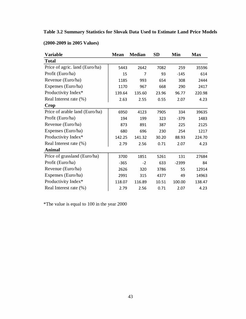
Table 3.2 Summary Statistics for Slovak Data Used to Estimate Land Price Models

(2000-2009 in 2005 Values)

*The value is equal to 100 in the year 2000


Price of agric. land (Euro/ha) 5443 2642 7082 259 35596

Profit (Euro/ha) 15 7 93 -145 614

Revenue (Euro/ha) 1185 993 654 308 2444

Expenses (Euro/ha) 1170 967 668 290 2417



Price of arable land (Euro/ha) 6950 4123 7905 334 39635

Profit (Euro/ha) 194 199 323 -379 1483

Revenue (Euro/ha) 873 891 387 225 2125

Expenses (Euro/ha) 680 696 230 254 1217



Price of grassland (Euro/ha) 3700 1851 5261 131 27684

Profit (Euro/ha) -365 -2 633 -2399 84

Revenue (Euro/ha) 2626 320 3786 55 12914

Expenses (Euro/ha) 2991 315 4377 49 14963



Total

Crop

Animal

44

Table 3.3 List of Variables

Variable Definition/computing Source

U.S. Slovakia

Price of

agricultural

land

Dependent variable The NASS

Quickstat

Buday, 2010

Profit Independent variable

Profit=Revenue –

Expenses

Deflation of profit

(Equation 9)

The ERS Statistic Office of

SR

Revenue Independent variable

Equations 1,2,3

Deflation of revenue

(Equation 9)

The ERS Statistic Office of

SR

Agroporadenstvo

Expenses Independent variable

Estimation based on data

from census year in the

whole U.S.

Deflation of expenses

(Equation 9)

The ERS

2007 Census of

Agriculture

Statistic Office of

SR

Agroporadenstvo

Rent Independent variable

Deflation of rent (Equat.

9)

The NASS -

Productivity

Index

Independent variable

Equations 4,5,6

The ERS

The USDA

Statistic Office of

SR

The Econ.

Research Inst.

Real Interest

Rate

Deflation of the interest

rate

Equation 10

Board of

Governors of the

Federal Reserve

System

Domestic credit

institutions

EU Dummy variable

Slovakia part of the EU

since the May 2004

EUit=0, if t=2000-2004;

otherwise EUit=1

- -

Fixed Effects Dummy variables:

16 states in U.S.

6 states in Slovakia

Stateit=1, if the

observation is for state i;

otherwise Stateit=0

- -

45

3.4 Methodology

Regression analysis is used estimate the model. The regression analysis explains

the relationship between variables, where one is called “the response, output or

dependent” variable and another one is called “the predictor, input, independent or

explanatory” variable. The dependent variable can only be continuous number, but the

independent variable can be continuous, categorical or discrete (Faraway, 2002).

There are two known regressions: simple regression, which shows the relationship

between one dependent and one independent variable, and multiple regression, which

explains the relationship between one dependent and more independent, explanatory

variables (Maddala, 2001). In my study I use multiple regression, where the model is:

Yi= α+ β1 x1i + β2 x2i +…+βk xki + ui, i=1,2,…,n (11)

To check for possible violations to the underlying assumptions of the ordinary

least squares (OLS) model, three different tests are performed. The tests performed check

for significant presence of:

Heteroskedasticity – “when the disturbances do not have the same variance”

Autocorrelation – “when the disturbances are correlated with one another‟‟

Multicollinearity- “two or more independent variables being approximately

linearly related in the sample data‟‟ (Kennedy, 2008).

Maddala (2001) describes six different assumptions about error ui

1. Linearity; E (ui)=0

2. Homoskedasticity; V (ui) = ζ2 for all i

3. No serial correlation; ui and uj are independent for all i≠j

4. Exogeneity; ui and xj are independent for all i and j

46

5. Normality; ui are normally distributed for all i

6. No linear dependences in the explanatory variables; α+ β1 x1i + β2 x2i +…+βk

xki=0

My model contains panel data so I use panel regression. The main difference

between time-series or cross-section regression is in using a double subscript on its

variables:

Yit=α + β1 Xit1 +β2 Xit2 +…+βk Xitk + uit, i=1,…,N; t=1,…,T (12)

where i can represent households, individuals or in our case states, and t represents the

time-series dimension (Baltagi, 2008).

As Baltagi (2008) explains „‟most of the panel data applications utilize a one–way

error model for the disturbances, with uit = μi + vit , where μi represents unobservable

individual specific effect and vit represents the remainder disturbance.‟‟

Kennedy (2008) sees advantages of using panel data in its possibilities in dealing

with heterogeneity in the micro units, combining variation across those units with

variation over time, and setting up more variability. The benefit of using panel data is it is

also better for analysis of dynamic adjustment and examining problems, which cannot be

studied by using only cross-sectional data or only time-series data.

Part of my model is created from fixed effects, which in my case are U.S. or

Slovak States. Baltagi (2008) sees the best reason to use the fixed effects model is that it

focuses on „‟a specific set of firms or states and our inference is restricted to the behavior

of these sets of firms or states.‟‟

47

3.4.1 Capitalization Model

The theoretical model used to select independent variables to explain the variation

in the dependent variable, land value, is the capitalization model:

Land Value = Expected net benefits / Discount rate

I adjusted this model for our variables:

Pijt= β1 E PROFijt+ β2 E PRODijt + β3 E INTERt + δ1 DS1 + δ2 DS2 +…+ δ16 DS16 + εijt

(13)

where

P is land value and is represented by the price of the land

E PROF is the expected net benefits and is represented by profitability

E PROD is the expected productivity and is represented by the productivity index

E INTER is the expected discount rate and is represented by the interest rate

DS is a dummy variable and is included for each state

i is used to indicate the particular state (16 states in U.S. and 6 states in Slovakia)

j is used to indicate the particular type of agriculture (crop, animal, and total)

t is used to indicate the year of the data (2000-2009)

ε is assumed to be normally distributed random error with mean zero and constant

variance.

A naïve expectations model is assumed for expected profit, expected productivity

and expected interest rate, where the previous year’s profit, productivity and interest rate

is assumed to equal their respective expected values. Therefore, profit, productivity and

interest rate are lagged one year and included in the model:

48

Pijt = β1 PROFijt-1+ β2 PRODijt-1 + β3 INTERt-1 + δ1 DS1 + δ2 DS2 +…+ δ16 DS16 + εijt

(14)

Then the variables land price, profit, productivity and interest rate are transformed by

taking their natural logarithm:

lnPijt= β1 ln PROFijt-1 + β2 ln PRODijt-1 + β3 ln INTERt-1 + δ1 DS1 + δ2 DS2 +…+ δ16

DS16 + εijt (15)

As the result of creating lagged variables, the land price for year 2000 is not

included in the estimated model.

In order to take the natural logarithm of the variables and run the regression

model, I had to adjust some variables which had negative values. It happened in four

cases. Profit had to be adjusted for the U.S. animal model by adding $420, for the SK

crop model by adding 380 Euro, for the SK animal model by adding 2400 Euro, and for

the SK total model by adding 145 Euro to each of the respective profit values.

In general, Land value = f (profitability, productivity, interest rate, and fixed

effects). Although the variables in equation (15) contain a j subscript to indicate three

separate types of agriculture (crop, animal, and total), a separate regression model is

estimated for each type of land j (cropland, pastureland, and total agricultural land).

Moreover, each of the regression models has four specifications, where the specifications

differ by the variable(s) used as a proxy for profitability. Specifically, the proxies for

profitability are either: 1) operating profit (crop, animal, or total), 2) revenue (crop,

animal, or total) and expenses (crop, animal, or total), 3) cash rent (crop, animal, or total),

or 4) output price index (crop, animal, or total) and input price index (crop, animal, or

total).

49

IV. EMPRICAL RESULTS

4.1 The Economic Software and Tests for Violations

At the beginning, I decided to use the econometric software – SAS Version 9.2 to

run the principal equations and test for multicollinearity, heteroscedasticity and

autocorrelation. I performed the test for multicollinearity (Appendix B, Tables 3 and 7)

and found that there is a non-harmful level of multicollinearity. The White test for

heteroscedasticity (Appendix B, Tables 1 and 5) failed to reject homoscedasticity. Later

on I changed to the econometric software – LIMDEP Version 9.0 (Greene, 2007). The

Durbin-Watson test for autocorrelation (Appendix B, Tables 2 and 6) supported the

conclusion that the errors are not autocorrelated for the Slovak models. However, the test

results indicated significant autocorrelation in the U.S. models. That was the main reason,

why I chose LIMDEP, which is better for running autocorrelation tests when using panel

data.

After a simple graphing of the residuals from a U.S. fixed effects model over

time, it is clearly seen that there are trends in the residuals over time and these trends are

consistent with positive autocorrelation. However, when I corrected the model for

autocorrelation, the sign of interest rate turns unexpectedly positive. I find this result

difficult to accept because of the theory, and graphical results show a negative

relationship between interest rate and land price. Both fixed effects without

autocorrelation and fixed effects with autocorrelation should be providing good estimates

of the parameters but the two methods are not doing so. Part of this could be assigned to

the short time-series of the samples for a given state and the fact of forcing the model to

estimate the same autocorrelation coefficient for each state. More expansive modeling

50

would allow the autocorrelation coefficients to vary across states but the software did not

support this. In addition, autocorrelation coefficients based on nine observations would

be suspect.

One source of autocorrelation is an omitted independent variable(s). I did try a

variety of independent variables (profit, productivity index, revenue and expenses) but

none seemed to eliminate the presence of autocorrelation. I have to accept this as a

shortcoming of the empirical results and leave it to other researchers to resolve this

problem. Finally I decided to run OLS without taking into consideration the presence of

autocorrelation yet recognizing it as a limitation. Although the coefficient estimates are

unbiased and consistent, the estimate of a coefficient’s variance is biased toward

downward. This could potentially result in rejecting the null hypothesis too frequently at

a given level of significance when, in fact, the result should be fail to reject. However, the

p-values found in this study when null hypotheses are rejected are quite low so that I

suspect the problem of autocorrelation is not severe.

In each of the following models, agricultural (crop, pasture or total) land is a

function of agricultural (crop, animal or total) profitability, agricultural (crop, animal or

total) productivity and interest rate. After lagging and taking the natural logarithm of the

continuous independent variables and including fixed effects, the model is:

Pijt= β1 ln PROFijt-1+ β2 ln PRODijt-1 + β3 ln INTERt-1 + δ1 DS1 + δ2 DS2 +…+ δ16 DS16 +

εijt

where P represents price of the land, PROF represents profit, PROD represents

productivity, INTER represents interest rate, DS represents dummy state variable, i

51

indicates 16 states in the U.S. and 6 states in Slovakia, j indicates crop, animal or total

agriculture, and t indicates the year of the data (2001-2009) .

4.2 U.S. Total Model with Profitability Proxied by Profit

The results of the estimated model when j = Total are reported in Table 4.1. The

R2 of the model is 92%, which means there is a very high proportion of the total

variability in the dependent variable, which is the price of agricultural land, is explained

by the independent variables. Adjusted R2 is 91% and is lower than the R

2 as expected.

The only statistically significant continuous variable in this model is the interest rate.

Since the continuous variables are in natural logarithms, the coefficient may be

interpreted an elasticity. A 1% increase in the interest rate would expect to result in a

decrease in the price of agricultural land of 0.56% (-0.56% change). Profit and

productivity index are not significant. A potential reason is that lagged profit may be a

poor proxy for expected profit. Another potential reason is inaccurate assumptions for the

allocation of expenses to arrive at profit, which was calculated as the difference between

revenue and expenses. Each of the estimated coefficients for the state dummy variables is

statistically significant. A test of the hypothesis that all the intercepts across states are

equal is rejected at the 0.0000 level. The coefficients on the state dummy variables are

interpreted as intercepts for the respective states. For example, the agricultural land price

for Arkansas is expected to be $1167 (e7.0620

) per acre if the values for all other

independent variables are set to zero.

52

Table 4.1 U.S. Total Model

4.3 U.S. Crop Model with Profitability Proxied by Profit

The results of the estimated model when j = Crop are reported in Table 4.2. Based

on R2, which measures the goodness model fit, it can be said that 92% of the total

variability of cropland price is explained by the independent variables. The fit of the

model is very good. Productivity and interest rate are significant variables. If there is a

1% increase in the productivity index, the price of cropland is expected to increase by

0.45%. If there is an increase in the interest rate of 1%, the price of cropland is expected

to decrease by 0.41% (-0.41% change). Profit, as in the model before, is not significant.

Based on the F test, the null hypothesis that all the coefficients equal zero is strongly

Ordinary least squares regression

Standard deviation 0.5166

Number of observations 144

Degrees of freedom 125

Residuals Sum of squares 3.0420

Standard error 0.1560

R-squared 0.9203

Adjusted R-squared 0.9088

Model test F [ 18, 125] (prob) 80.16 (.0000)

Variable Coefficient Standard Error t-ratio P[|T|>t] Mean of X

LAGPROF 0.0117 0.0364 0.3200 0.7496 4.7739

LAGPROD 0.2449 0.1635 1.4980 0.1367 4.6612

LAGINTER -0.5647 0.1052 -5.3700 0.0000 1.4867

AR 7.0620 0.8058 8.7640 0.0000 0.0625

GA 7.5767 0.7867 9.6310 0.0000 0.0625

IL 7.6644 0.7938 9.6550 0.0000 0.0625

IN 7.6438 0.7934 9.6340 0.0000 0.0625

IA 7.4413 0.7971 9.3350 0.0000 0.0625

KS 6.2983 0.7939 7.9330 0.0000 0.0625

LA 7.0114 0.8074 8.6840 0.0000 0.0625

MN 7.1978 0.7916 9.0920 0.0000 0.0625

MS 6.9579 0.8149 8.5380 0.0000 0.0625

MO 7.0759 0.7914 8.9400 0.0000 0.0625

NE 6.4365 0.8019 8.0270 0.0000 0.0625

NC 7.7776 0.7944 9.7900 0.0000 0.0625

OK 6.3608 0.7938 8.0140 0.0000 0.0625

TN 7.5284 0.8021 9.3860 0.0000 0.0625

TX 6.4997 0.7957 8.1690 0.0000 0.0625

WI 7.5174 0.7892 9.5260 0.0000 0.0625

53

rejected. A test of the hypothesis that all the intercepts across states are equal is rejected

at the 0.0000 level (Appendix B, Table 4).

Table 4.2 U.S. Crop Model

4.4 U.S. Animal Model with Profitability Proxied by Profit

The results of the estimated model when j = Animal are reported in Table 4.3.

Based on R2, which is 91%, it can be said that there is a good fit of the model. Profit is

significant. The problem is that the result indicates that if there is a 1% increase in profit,

the price of pastureland is expected to decrease by 0.39% (-0.39% change). This result is

not in accordance with previous studies described in the literature review, which say an







R-squared 0.9224


Model test [ 18, 125] (prob) = 82.60 (.0000)82.6 (.00000)


LAGPROF 0.0154 0.0740 0.2070 0.8360 5.3248

LAGPROD 0.4526 0.1462 3.0960 0.0024 4.6987

LAGINTER -0.4114 0.1003 -4.1000 0.0001 1.4867

AR 5.6270 0.7435 7.5680 0.0000 0.0625

GA 6.3380 0.7402 8.5630 0.0000 0.0625

IL 6.5160 0.7256 8.9800 0.0000 0.0625

IN 6.4536 0.7301 8.8400 0.0000 0.0625

IA 6.3365 0.7308 8.6700 0.0000 0.0625

KS 5.1000 0.7214 7.0700 0.0000 0.0625

LA 5.6502 0.7402 7.6330 0.0000 0.0625

MN 6.0030 0.7141 8.4060 0.0000 0.0625

MS 5.5415 0.7564 7.3260 0.0000 0.0625

MO 5.9782 0.7145 8.3670 0.0000 0.0625

NE 5.6842 0.7359 7.7240 0.0000 0.0625

NC 6.5477 0.7205 9.0880 0.0000 0.0625

OK 5.1640 0.7076 7.2980 0.0000 0.0625

TN 6.2720 0.7351 8.5330 0.0000 0.0625

TX 5.3641 0.7376 7.2730 0.0000 0.0625

WI 6.3326 0.7113 8.9030 0.0000 0.0625

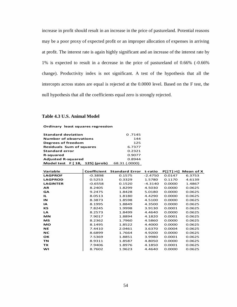
54

increase in profit should result in an increase in the price of pastureland. Potential reasons

may be a poor proxy of expected profit or an improper allocation of expenses in arriving

at profit. The interest rate is again highly significant and an increase of the interest rate by

1% is expected to result in a decrease in the price of pastureland of 0.66% (-0.66%

change). Productivity index is not significant. A test of the hypothesis that all the

intercepts across states are equal is rejected at the 0.0000 level. Based on the F test, the

null hypothesis that all the coefficients equal zero is strongly rejected.

Table 4.3 U.S. Animal Model


Standard deviation 0 .7145





R-squared 0.9077


Model test F [ 18, 125] (prob) 68.31 (.0000)


LAGPROF -0.3898 0.1575 -2.4750 0.0147 6.3753

LAGPROD 0.5253 0.3329 1.5780 0.1170 4.6139

LAGINTER -0.6558 0.1520 -4.3140 0.0000 1.4867

AR 8.2405 1.8299 4.5030 0.0000 0.0625

GA 9.2475 1.8428 5.0180 0.0000 0.0625

IL 8.0513 1.8180 4.4290 0.0000 0.0625

IN 8.3873 1.8598 4.5100 0.0000 0.0625

IA 8.1995 1.8849 4.3500 0.0000 0.0625

KS 7.8245 1.9998 3.9130 0.0001 0.0625

LA 8.2573 1.8499 4.4640 0.0000 0.0625

MN 7.9017 1.8894 4.1820 0.0001 0.0625

MS 8.2362 1.7960 4.5860 0.0000 0.0625

MO 8.1495 1.8522 4.4000 0.0000 0.0625

NE 7.4410 2.0461 3.6370 0.0004 0.0625

NC 8.6899 1.7664 4.9200 0.0000 0.0625

OK 7.5369 1.8851 3.9980 0.0001 0.0625

TN 8.9311 1.8587 4.8050 0.0000 0.0625

TX 7.9406 1.8976 4.1850 0.0001 0.0625

WI 8.7602 1.9623 4.4640 0.0000 0.0625

55

4.5 U.S. Total Model with Profitability Proxied by Revenues and Expenses

The results of the estimated model when j = Total are reported in Table 4.4. The

model is showing the relationship between the price of agricultural land and total

profitability proxied by revenue and expenses, total productivity and interest rate. R2 is

95% and is higher than adjusted R2 as expected. Greater amount of variation in

agricultural land price is explained by independent variables when revenues and expenses

are included as proxies of profitability than when profit is included as a proxy of

profitability as was reported earlier. Revenue and interest rate are highly significant. An

increase of revenue by 1% is expected to result in an increase in the price of agricultural

land of 1.04% (1.04% change). If there is an increase in the interest rate of 1%, the price

of agricultural land is expected to decrease by 0.40% (-0.40% change). Productivity

index and expenses are not significant. Most of the estimated coefficients for the state

dummy variables are statistically significant. A test of the hypothesis that all the

intercepts across states are equal is rejected at the 0.0000 level.

56

Table 4.4 U.S. Total Model

4.6 U.S. Crop Model with Profitability Proxied by Revenues and Expenses

The results of the estimated model when j = Crop are reported in Table 4.5. The

results show the relationship between the price of cropland and crop revenue, crop

expenses, crop productivity index and interest rate. R2 is 96%, which again means that

even a greater amount of variation in cropland price is explained by independent

variables when revenues and expenses are included as proxies of profitability. All

independent variables in this model are significant. If there is an increase in the revenue

of 1%, the price of cropland will increase by 0.79% (0.79% change). If there is an

increase in expenses of 1%, the price of cropland will decrease by 0.31% (-0.31 change).







R-squared 0.9509


Model test F [ 19, 124] (prob) 126.52 (.0000)


LAGREV 1.0376 0.1574 6.5930 0.0000 6.0524

LAGEXP -0.0753 0.1438 -0.5240 0.6015 6.3171

LAGPROD 0.1025 0.1302 0.7870 0.4329 4.6612

LAGINTER -0.4021 0.0860 -4.6770 0.0000 1.4867

AR 1.8014 0.8846 2.0360 0.0438 0.0625

GA 1.6577 0.9343 1.7740 0.0785 0.0625

IL 2.5160 0.8657 2.9060 0.0043 0.0625

IN 2.3656 0.8768 2.6980 0.0079 0.0625

IA 2.0063 0.8919 2.2500 0.0262 0.0625

KS 1.0135 0.8754 1.1580 0.2492 0.0625

LA 1.8600 0.8746 2.1270 0.0354 0.0625

MN 1.9712 0.8711 2.2630 0.0254 0.0625

MS 1.5637 0.9000 1.7370 0.0848 0.0625

MO 2.3762 0.8289 2.8670 0.0049 0.0625

NE 0.8726 0.9047 0.9650 0.3367 0.0625

NC 1.6062 0.9593 1.6740 0.0966 0.0625

OK 1.4103 0.8496 1.6600 0.0995 0.0625

TN 2.5211 0.8570 2.9420 0.0039 0.0625

TX 1.2152 0.8807 1.3800 0.1701 0.0625

WI 2.0678 0.8890 2.3260 0.0216 0.0625

57

An increase in the productivity index by 1% is expected to result in an increase in the

price of cropland of 0.39% (0.39% change). An increase in the interest rate by 1% is

expected to result in a decrease in the price of cropland by 0.21% (-0.21% change). A test

of the hypothesis that all the intercepts across states are equal is rejected at the 0.0000

level. Each of the estimated coefficients for the state dummy variables is statistically

significant.

Table 4.5 U.S. Crop Model







R-squared 0.9550


Model test F [ 19, 124] (prob) 138.42 (.0000)


LAGREV 0.7858 0.0894 8.7910 0.0000 4.5821

LAGEXP -0.3119 0.0938 -3.3270 0.0012 5.7200

LAGPROD 0.3865 0.1120 3.4510 0.0008 4.6987

LAGINTER -0.2125 0.0796 -2.6710 0.0086 1.4867

AR 3.9227 0.6112 6.4180 0.0000 0.0625

GA 4.2471 0.6228 6.8190 0.0000 0.0625

IL 4.7378 0.6008 7.8860 0.0000 0.0625

IN 4.7331 0.6047 7.8270 0.0000 0.0625

IA 4.6343 0.6016 7.7040 0.0000 0.0625

KS 3.6759 0.5833 6.3020 0.0000 0.0625

LA 3.7906 0.6146 6.1680 0.0000 0.0625

MN 4.2930 0.5883 7.2970 0.0000 0.0625

MS 3.6955 0.6244 5.9190 0.0000 0.0625

MO 4.3824 0.5844 7.4980 0.0000 0.0625

NE 4.0781 0.6016 6.7780 0.0000 0.0625

NC 4.5506 0.6064 7.5050 0.0000 0.0625

OK 3.7382 0.5728 6.5260 0.0000 0.0625

TN 4.4952 0.6059 7.4190 0.0000 0.0625

TX 3.7846 0.6012 6.2950 0.0000 0.0625

WI 4.6354 0.5862 7.9080 0.0000 0.0625

58

4.6 U.S. Animal Model with Profitability Proxied by Revenues and Expenses

The results of the estimated model when j = Animal are reported in Table 4.6. The

model shows the relationship between pastureland and the animal profitability,

productivity and interest rate. R2 is 0.96 which means that 96% of variability in price of

pastureland is explained by independent variables. There are two significant variables

which are revenue and interest rate. If there is an increase of the revenue by 1%, there

will be an increase in the price of pastureland by 2.22% (2.22% change). The revenue has

a really strong impact on the price of pastureland. Another significant variable, which is

the interest rate, is positive. It indicates that if the interest rate increases by 1%, the price

of pastureland will increase by 0.34% (0.34% change), which is not in accordance with

previous literature. Expenses and productivity are not significant. Most of the estimated

coefficients for the state dummy variables are statistically significant. A test of the

hypothesis that all the intercepts across states are equal is rejected at the 0.0000 level.

59

Table 4.6 U.S. Animal Model







R-squared 0.9597


Model test F [ 19, 124] (prob) 155.51 (.0000)


LAGREV 2.2213 0.1694 13.1120 0.0000 5.4530

LAGEXP -0.1257 0.1294 -0.9710 0.3335 5.9076

LAGPROD 0.0421 0.2240 0.1880 0.8511 4.6139

LAGINTER 0.3397 0.1278 2.6570 0.0089 1.4867

AR -3.7240 1.3460 -2.7670 0.0065 0.0625

GA -3.7970 1.4264 -2.6620 0.0088 0.0625

IL -6.5781 1.5357 -4.2830 0.0000 0.0625

IN -5.7589 1.5112 -3.8110 0.0002 0.0625

IA -6.7827 1.5677 -4.3270 0.0000 0.0625

KS -7.3777 1.6278 -4.5320 0.0000 0.0625

LA -3.3439 1.3416 -2.4920 0.0140 0.0625

MN -6.1353 1.5165 -4.0460 0.0001 0.0625

MS -3.9125 1.3280 -2.9460 0.0038 0.0625

MO -2.3656 1.3067 -1.8100 0.0727 0.0625

NE -8.8289 1.6985 -5.1980 0.0000 0.0625

NC -5.5072 1.4939 -3.6860 0.0003 0.0625

OK -3.1191 1.3574 -2.2980 0.0232 0.0625

TN -1.8360 1.3199 -1.3910 0.1667 0.0625

TX -3.8406 1.4176 -2.7090 0.0077 0.0625

WI -4.9913 1.5440 -3.2330 0.0016 0.0625

60

Table 4.7 Summary of U.S. Models

*Statistically significant at the 0.10 level

**Statistically significant at the 0.05 level

***Statistically significant at the 0.01 level

Model with profit as a measure of

profitability

Model with revenue and expenses as a

measure of profitability

Price of land Price of land

Land

Expl. variables

Agricul. Crop Pasture

Agricul. Crop Pasture

Profit 0.01 0.01 -0.38** - - -

Revenue - - - 1.03*** 0.78*** 2.22***

Expenses - - - -0.07 -0.31*** -0.12

Prod. index 0.24 0.45*** 0.52 0.10 0.38*** 0.04

Interest rate -0.56*** -0.41*** -0.65*** -0.40*** -0.21*** 0.33***

AR 7.06*** 5.62*** 8.24*** 1.80** 3.92*** -3.72***

GA 7.57*** 6.33*** 9.24*** 1.65** 4.24*** -3.79***

IL 7.66*** 6.51*** 8.05*** 2.51*** 4.73*** -6.57***

IN 7.64*** 6.45*** 8.38*** 2.36*** 4.73*** -5.75***

IA 7.44*** 6.33*** 8.19*** 2.00*** 4.63*** -6.75***

KS 6.29*** 5.10*** 7.82*** 1.01 3.67*** -7.37***

LA 7.01*** 5.65*** 8.25*** 1.85*** 3.79*** -3.34**

MN 7.19*** 6.00*** 7.70*** 1.97*** 4.29*** -6.13***

MS 6.95*** 5.54*** 8.23*** 1.56** 3.69*** -3.91***

MO 7.07*** 5.97*** 8.14*** 2.37*** 4.38*** -2.36**

NE 6.43*** 5.68*** 7.44*** 0.87 4.07*** -8.82***

NC 7.77*** 6.54*** 8.68*** 1.60* 4.55*** -5.50***

OK 6.36*** 5.16*** 7.53*** 1.41* 3.73*** -3.11**

TN 7.52*** 6.27*** 8.93*** 2.52*** 4.49*** -1.83

TX 6.49*** 5.36*** 7.94*** 1.21 3.78*** -3.84***

WI 7.51*** 6.33*** 8.76*** 2.06** 4.63*** -4.99***

R2 0.92 0.92 0.91 0.95 0.95 0.96

Adjusted R2 0.91 0.91 0.89 0.94 0.95 0.95

61

Based on R2, the goodness of fit for the models is very good (Table 4.7). The

proportion of total variability in the dependent variable, which is the price of land, is

explained by the independent variables in all six models is quite high at 91% or more.

Profit as a measure of profitability is significant in only one of three models, and

then it is unexpectedly negative. In contrast, in models with profitability measured by

revenue and expenses, revenue is highly significant and positive as expected in all three

models. Expenses are only significant in its relationship with the price of cropland and

the relationship is negative as expected. The insignificance of expenses in the other two

models may be, as mentioned before, explained by inaccurate allocation of the expenses.

The productivity index only shows significance in the case of crop productivity in

both cropland price models.

The interest rate is significant in all six models. However, it has an unexpectedly

positive sign in the pastureland price model when revenue and expenses are used as a

measure of profitability.

4.7 SK Total Model with Profitability Proxied by Profit

The results of the estimated model when j = Total are reported in Table 4.8. Based

on R2

which is 62%, we can say is a high proportion of total variability in the dependent

variable, which is the price of agricultural land, is explained by the independent variables.

As expected R2 is higher than adjusted R

2. The fit of the Slovak model is not as good as

in the U.S. models. The only significant variable is interest rate. Since the continuous

variables are in natural logarithms, the interpretation of the coefficient is that of elasticity.

If there is an increase of the interest rate by 1%, agricultural land will decrease by 1.72%

62

(-1.72% change). Profit and the productivity index are not significant. The EU variable is

included to test if there is any impact on land values from Slovakia joining the EU in

May 2004. The EU variable equals 0 if t equal 2000-2004, and 1 otherwise. Since the

estimate of the EU coefficient is statistically insignificant, the impact is not significant. A

test of the hypothesis that all the intercepts across states are equal is rejected at the 0.0000

level.

It is important to mention that in the case of Slovakia, the data appear to be very

inaccurate. As it was explained in the literature review, the statistical networks are not

very functional and there is a question of the reliability of the data obtained from the

official statistic sources. Especially suspect are land price data since they have

unexplainably large changes between the years. That is why I do not really trust results I

got in any of the Slovak models.

63

Table 4.8 SK Total Table

4.8 SK Crop Model with Profitability Proxied by Profit

The results of the estimated model when j = Crop are reported in Table 4.9. The

model reflects the relationship between the price of cropland and crop profit, crop

productivity index and interest rate in Slovakia. R2 is 0.68, which means that 68% of

variability in dependent variable, which is arable land, is explained by independent

variables. The only significant variable is the interest rate. If there is an increase of the

interest rate by 1%, the price of cropland will decrease by 1.95% (-1.95% change). Profit,

productivity index and the EU variable are insignificant. A test of the hypothesis that all

the intercepts across states are equal is rejected at the 0.0000 level (Appendix B, Table 8).







R-squared 0.6240


Model test F [ 8, 45] (prob) 9.34 (.0000)


LAGPROF -0.2610 0.4227 -0.6180 0.5400 4.9732

LAGPROD 0.1904 0.9252 0.2060 0.8379 4.8794

LAGINTER -1.7161 0.6937 -2.4740 0.0173 1.0277

EU -0.1071 0.3501 -0.3060 0.7612 0.5556

DS 11.1349 4.5008 2.4740 0.0173 0.1667

TO 9.9764 4.5674 2.1840 0.0343 0.1667

LM 11.4515 4.4494 2.5740 0.0135 0.1667

RS 9.2052 4.6322 1.9870 0.0531 0.1667

SK 9.5621 4.6642 2.0500 0.0463 0.1667

MI 10.4588 4.5239 2.3120 0.0255 0.1667

64

Table 4.9 SK Crop Model

4.9 SK Animal Model with Profitability Proxied by Profit


Based on R2, in the model, 67% of the variability in the dependent variable, which is the

price of pastureland, is explained by the independent variables, which are animal

revenue, expenses, productivity index and interest rate. The only significant variables are

profit and EU. If there is an increase in profit by 1%, the price of pastureland decreases

by 0.21% (-0.21% change). This result is not in accordance with previous studies

described in the literature review, which say an increase in profit should result in an

increase in the price of pastureland. Productivity is not significant. The variable EU

shows significance and it is negative, which indicates that after Slovakia became part of







R-squared 0.6822


Model test F [ 9, 44] (prob) 10.49 (.0000)


LAGPROF 0.2364 0.3372 0.7010 0.4869 6.3103

LAGPROD -0.7488 0.8122 -0.9220 0.3616 4.9199

LAGINTER -1.9575 0.6845 -2.8600 0.0065 1.0277

EU -0.0237 0.3844 -0.0620 0.9511 0.5556

DS 13.3542 3.4421 3.8800 0.0003 0.1667

TO 12.2357 3.4801 3.5160 0.0010 0.1667

LM 13.5977 3.3380 4.0740 0.0002 0.1667

RS 11.4205 3.5387 3.2270 0.0024 0.1667

SK 12.2624 3.5512 3.4530 0.0012 0.1667

MI 12.9478 3.5398 3.6580 0.0007 0.1667

65

the EU, there was a decrease in the price of pastureland. A test of the hypothesis that all

the intercepts across states are equal is rejected at the 0.0000 level.

Table 4.10 SK Animal Model

4.10 SK Total Model with Profitability Proxied by Revenues and Expenses

The results of the estimated model when j = Total are reported in Table 4.11.

Based on R2, 67% of the variation in the dependent variable, which is the price of

agricultural land, is explained by the independent variables, which are the total revenue,

expenses, productivity index and interest rate. And the R2 is higher than adjusted R

2 as

expected. As indicated by the adjusted R2s from the two SK total agricultural land

models, a greater proportion of the variation in agricultural land price is explained by







R-squared 0.6684


Model test F [ 8, 45] (prob) 11.34 (.0000)


LAGPROF -0.2112 0.0975 -2.1660 0.0357 7.4152

LAGPROD 3.2360 2.4363 1.3280 0.1909 4.7609

LAGINTER -1.5971 0.9700 -1.6460 0.1068 1.0277

EU -0.5620 0.3089 -1.8200 0.0756 0.5556

DS -3.7385 12.3800 -0.3020 0.7641 0.1667

TO -3.9808 12.4469 -0.3200 0.7506 0.1667

LM -3.0585 12.4977 -0.2450 0.8078 0.1667

RS -5.1207 12.4615 -0.4110 0.6831 0.1667

SK -4.6838 12.3677 -0.3790 0.7067 0.1667

MI -4.4536 12.4472 -0.3580 0.7222 0.1667

66

independent variables when revenues and expenses are included as proxies of

profitability than when profit is included as a proxy of profitability. The only significant

variable is the interest rate. If there is an increase in the interest rate by 1%, the price of

agricultural land will decrease by 1.73% (-1.73% change). All other variables like

revenue, expenses, productivity index and the EU variable are not significant. A test of

the hypothesis that all the intercepts across states are equal is rejected at the 0.0000 level.

Table 4.11 SK Total Model

4.11 SK Crop Model with Profitability Proxied by Revenues and Expenses

The results of the estimated model when j = Crop are reported in Table 4.12.


cropland, is explained by independent variables, which are crop revenue, expenses,







R-squared 0.6738


Model test F [ 10, 43] (prob) 8.88 (.0000)


LAGREV 4.8094 3.9367 1.2220 0.2285 6.9136

LAGEXP -4.9129 3.9167 -1.2540 0.2165 6.9232

LAGPROD 0.7178 1.0494 0.6840 0.4976 4.8794

LAGINTER -1.7336 0.6900 -2.5130 0.0158 1.0277

EU -0.0929 0.3420 -0.2720 0.7871 0.5556

DS 8.1152 8.2817 0.9800 0.3326 0.1667

TO 6.9280 8.2880 0.8360 0.4078 0.1667

LM 8.3995 7.7186 1.0880 0.2826 0.1667

RS 6.0772 7.9309 0.7660 0.4477 0.1667

SK 6.3611 7.3255 0.8680 0.3900 0.1667

MI 7.3140 7.6728 0.9530 0.3458 0.1667

67

productivity index and interest rate. The only significant variable is the interest rate. If

there is an increase of the interest rate by 1%, the price of cropland will decrease by

2.00% (-2.00% change). Revenue, expenses, productivity index and the EU variable are

not significant. A test of the hypothesis that all the intercepts across states are equal is

rejected at the 0.0000 level.

Table 4.12 SK Crop Model

4.12 SK Animal Model with Profitability Proxied by Revenues and Expenses



pastureland, is explained by the independent variables, which are animal revenue,

expenses, productivity index and interest rate. The only significant variable in model is







R-squared 0.6893


Model test F [ 10, 43] (prob) 3.87 (.0015)


LAGREV -0.2958 0.6624 -0.4470 0.6574 6.4507

LAGEXP 0.7042 0.6473 1.0880 0.2827 6.7238

LAGPROD -0.9617 0.8383 -1.1470 0.2577 4.9199

LAGINTER -2.0007 0.6731 -2.9720 0.0048 1.0277

EU 0.1119 0.4023 0.2780 0.7822 0.5556

DS 12.9591 6.0593 2.1390 0.0382 0.1667

TO 11.8039 6.2000 1.9040 0.0636 0.1667

LM 13.0835 6.0771 2.1530 0.0370 0.1667

RS 11.0738 5.9737 1.8540 0.0706 0.1667

SK 12.2217 5.4733 2.2330 0.0308 0.1667

MI 12.7652 5.7163 2.2330 0.0308 0.1667

68

productivity. If there is an increase in the productivity index by 1%, the price of

pastureland will increase by 6.00% (6.00% change). The rest of the variables are not

significant. A test of the hypothesis that all the intercepts across states are equal is

rejected at the 0.0000 level.

Table 4.13 SK Animal Model







R-squared 0.6483


Model test F[ 10, 43] (prob) 7.93 (.0000)


LAGREV -0.0382 1.7615 -0.0220 0.9828 6.5298

LAGEXP 1.2404 2.2648 0.5480 0.5867 6.5419

LAGPROD 5.9974 2.9615 2.0250 0.0491 4.7609

LAGINTER -0.9304 1.0453 -0.8900 0.3784 1.0277

EU -0.2645 0.4213 -0.6280 0.5334 0.5556

DS -30.0313 20.8069 -1.4430 0.1562 0.1667

TO -29.8913 20.4218 -1.4640 0.1505 0.1667

LM -25.9101 18.6276 -1.3910 0.1714 0.1667

RS -27.3416 18.2228 -1.5000 0.1408 0.1667

SK -25.7408 17.5268 -1.4690 0.1492 0.1667

MI -26.6946 18.1881 -1.4680 0.1495 0.1667

69

Table 4.14 Summary of Results for SK Models

*Statistically significant at the a=0.10 level

**Statistically significant at the a=0.05 level

***Statistically significant at the a=0.01 level

Even if I do not have confidence in the results provided by the Slovak models

because of inaccurate data, they show significance of the interest rate in the total and crop

Model with profit as a measure of

profitability

Model with revenue and expenses as

measures of profitability

Price of land Price of land

Land

Explanatory variables

Agricultural Arable Pasture

Agricultural Arable Pasture

Profit -0.26 0.23 -0.21** - - -

Revenue - - - 4.80 -0.30 -0.03

Expenses - - - -4.91 0.70 1.24

Productivity index 0.19 -0.74 3.23 0.71 -0.96 5.99**

Interest rate -1.71*** -1.95*** -1.59 -1.73*** -2.00*** -0.93

EU -0.10 -0.02 -0.56** -0.09 0.78 -0.26

DS 11.13 13.35*** -3.73 8.11 12.96* -30.03

TO 9.97 12.24*** -3.98 6.92 11.80* -29.89

LM 11.45 13.60*** -3.05 8.39 13.08* -25.91

RS 9.20 11.42*** -5.12 6.07 11.07* -27.34

SK 9.56 12.26*** -4.68 6.36 12.22* -25.74

MI 10.45 12.94*** -4.45 7.31 12.77* -26.69

R2 0.69 0.68 0.67 0.67 0.69 0.65

Adjusted R2 0.66 0.62 0.60 0.60 0.62 0.57

70

models. There are only three other significant variables in all Slovak models. Profit and

the EU variable are significant in animal model with profitability proxied by profit, but

profit has an unexpected negative sign. The other significant variable is the productivity

index, which is positive as expected, in animal model with profitability proxied by

revenue and expenses.

71

V. SUMMARY AND CONCLUSION

In this study, three null hypotheses are tested:

1. Agricultural land (cropland or pastureland) value is not related to agricultural

(crop or animal) profitability.

2. Agricultural land (cropland or pastureland) value is not related to agricultural

(crop or animal) productivity.

3. Agricultural land (cropland or pastureland) is not related to interest rate.

All U.S. model results fail to reject the first hypothesis when profit is used as a

proxy for profitability. When revenue and expenses are used as proxies for profitability,

support for the theory is for the most part improved. In the case of revenue, the null

hypothesis is rejected and the alternative hypothesis that revenue has a positive impact on

land price is accepted. In the case of expenses, the null hypothesis is only rejected in the

cropland model of the three models and the alternative hypothesis of a negative impact on

land price is accepted.

The second null hypothesis about no relationship between land price and

productivity is failed to be rejected in the total agricultural land and pastureland models.

However, this hypothesis is rejected and the alternative hypothesis is accepted in the

cropland price models where there is a significant, positive relationship with crop

productivity.

The third null hypothesis is consistently rejected. There is a significant, negative

relationship between interest rate and land price in five of the six U.S. models. The lone

72

exception is for the pasture land model when revenue and expenses are used to proxy

profitability.

In the case of Slovak models, the first and second hypotheses are failed to be

rejected in favor of the alternative hypotheses in all but one case. In that case, the

alternative hypothesis of pastureland price is positively related to animal productivity is

accepted when revenue and expenses are used as a proxy for profitability.

The third null hypothesis is rejected in favor of the alternative hypothesis that

land values are negatively related to interest rates in four of the six models. The

exceptions are the pastureland price models where the interest rate is statistically

insignificant.

It is important to say that I do not trust the Slovak model results because of I

suspect data are inaccurate. The way of collecting land value data is not very functional.

There are huge differences in the values between years, and there are very high values in

some states. The high prices may be explained by new investors coming to Slovakia

during the ten-year period and buying agricultural land for new factories. Subsequently,

the price of the agricultural land increases rapidly. Unfortunately, this is not an

explanation for all states and for the high variability over the years. The high variability

could be explained by investors repeatedly entering and exiting the Slovakian market.

However, this explanation seems unlikely. The fluctuation in price can also be caused by

the unstable legislation, which is frequently changing according to the particular

government holding office.

A law that regulates the uses of the land, forces the buyers to pay extra fees if they

are planning to change the use of the land, for example, from agricultural land to a

73

construction site. This law has had a negative effect on the prices of land, where on one

side buyers do not want to pay for the elevated extra fees and on the other side

landowners negotiate lower prices in order to be able to sell their land. (Bandlerova,

personal communication, June, 29, 2011)

I also had problems with getting data for profitability, where I had to make

assumptions for allocating expenses between crop and animal production since only total

expenses were reported. Even after e-mail communication with six different regional

statistical offices, they were not able to provide the data needed, because “these data are

not collected or calculated at state level”. Even after Slovakia became part of the

European Union in 2004 and the statistical networks have developed because of the EU

requirements, collecting data on regional or state levels still needs to be improved.

Collecting and monitoring data just on a country level or, in some cases, on a regional

level makes it difficult to do analysis and provide recommendations for solving problems

experienced at the smaller state levels.

The main problem to deal with in collecting information for the U.S. model was

in allocating expenses. There are not data reported separately for crop production

expenses and animal production expenses. The insignificance for some the results may be

because of improper assumptions regarding the allocation of expenses. It would be very

useful if the USDA would provide this kind of information.

In the U.S. models, I also had to deal with violation of the non-autocorrelation

assumption and the difficulty in correcting for this violation, which may be attributable to

the shortness of the sample, where only nine years were used in estimating the models.

Unfortunately, there was not enough data for including previous years. The lack of time

74

series data was also the case for Slovakia. Data on state land prices are not available from

years before 2000.

It would be interesting to repeat this study in the future with additional years and

maybe with additional states and with more accurate data. Also of interest may be to

include additional independent variables, such as unemployment rates and measures of

wealth and liquidity. Finally, it would be interesting to focus on disaggregated data from

one state and to collect more variables that may have an impact on land prices. This may

result in more precise estimates in support of the impact of profitability, productivity and

interest rate on agricultural land price.

75

VI. BIBLIOGRAPHY

Aakre, D., and H. Vreugdenhil. 2004. “Results of North Dakota Land Valuation Model

for the 2004 Agricultural Real Estate Assessment.” AgEcon Search.

http://ageconsearch.umn.edu/bitstream/23666/1/sp040003.pdf Last accessed:

November 2, 2010.

Ahearn M., and R. Alig. 2005a. “A Discussion of Recent Land-Use Trends”. Chapter 2.In

Economics of Rural Land-Use Change. Burlington. Ashagate Publishing Limited,

pp.12-25.

Ahearn M., and R. Alig. 2005b. “Effects of Policy and Technological Change on Land

Use”. Chapter 3. In Economics of Rural Land-Use Change. Burlington. Ashagate

Publishing Limited, pp25-37.

Ahrendsen, B. L. 2000. “Slovak Farm Financial Problems: Profitability, Debt, Late

Payment, and Lack of Credit. Technical assistance report to the Ministry of

Agriculture Slovak Republic”. AgEcon Search. pp. 11.

http://ageconsearch.umn.edu/bitstream/15779/1/sp132000.pdf Last

accessed: October 5, 2010.

Alston, J. 1986. “An Analysis of Growth of U.S. Farmland Prices in 1963-82”. American

Journal of Agricultural Economics, 86(68, 1):1-9. http://0-

web.ebscohost.com.library.uark.edu/ehost/pdfviewer/pdfviewer?vid=5&hid=13&

sid=f76cb6d8-56b2-4014-9038-f917639d1075%40sessionmgr4 Last accessed:

November 2, 2010.

Baltagi, B. 2008. “Econometrics Analysis of Panel Data”. 4th ed. John Wiley and sons

Ltd. Sussex.

Bandlerova, A. 2005. “Some Reasons that Influence Agrarian Land Market”. Slovak

Agricultural University in Nitra. FAO PowerPoint presentation Nitra,Slovakia. 6-

7- May.

Bandlerova, A., and J. Lazikova. 2005a. “Some Reasons that Influence Agrarian Land

Market Development-Case of Slovakia”. Development of Land Markets and

Related Institutions In Countries of Central And Eastern Europe. FAO Regional

Workshop Nitra ,Slovakia. 6-7- May.

Bandlerova, A., and J. Lazikova. 2005b. “Agricultural Land Tenure”. Slovak Agricultural

University. Nitra. Acta Regionalia et Environmentalica Journal .05(2,2): 29-34.

Bandlerová A., and J. Lazikova. 2009. “Agricultural Land Lease in Slovakia”. Il Diritto

Dell'Agricoltura : rivista quadrimestrale diretta da Felice Casucci. - Napoli :

Edizioni Scientifiche Italiane, 09(1):65-81.

http://ageconsearch.umn.edu/bitstream/23666/1/sp040003.pdf

http://ageconsearch.umn.edu/bitstream/15779/1/sp132000.pdf

http://0-web.ebscohost.com.library.uark.edu/ehost/pdfviewer/pdfviewer?vid=5&hid=13&sid=f76cb6d8-56b2-4014-9038-f917639d1075%40sessionmgr4



http://agris.fao.org/?query=%2BcitationTitle:%22Acta%20Regionalia%20et%20Environmentalica%22

76

Bandlerova, A., J. Lazikova, and L. Rumanovska. 2005a. “Agricultural Land Ownership

and Lease Problems: Slovakia Case Study”. Referat na medzinarodnom vedeckom

seminari v Kakowe 16.-17.11.2005 sekcia Przemiany Demograficzne, kulturove,

bezrobocie I aktzwizacia zawodowa na obszarach wiejskich. Krakow.

Bandlerova, A., J. Lazikova, and L. Rumanovska . 2005b. “Agricultural Land Tenure-

Case of Slovakia”. The Impact of European Inegration on the National Economy

Conference. Cluj-Napoca Romania.

Bandlerova, A., and E. Marisova. 2000. “Legal Regulations Pertaining To Agricultural

Land In Slovakia And Their Influence On Rural Development”. In David Brown

and Anna Bandlerová: Rural Development in Central and Eastern Europe 2000,

pp. 129-134.

Bandlerova ,A., and E. Marisova. 2003. “Importance of Ownership and Lease of

Agricultural Land in Slovakia in the Pre-accession Period”. Agricultural

Economics. 03(49,5) :213 – 216.

Bandlerova, A., E. Marisova, and M. Stefanovic. 2002. “Land Ownership Fragmentation

and Problems with Use of Agricultural Land: Case of Slovakia”. Conference:

Land registration and spatial planning in transition countries: opportunities for

the European Union? .Wageningen. Holand. 31.October-1.November 2002.

Wageningen University, Environmental Policy Group. pp. 193-207.

Bandlerova, A., P. Schwarcz, and E.Marisova. 2011. “Držba Pôdy a Rozvoj Vidieka na

Slovensku. Land Tenure and Rural Development –Case Slovakia”. Working

paper. Slovak Agricultural University. Nitra.

Blaas,G. 2001. “Agricultural Reform in Slovakia: Changing Institutions and Structure”.

Ieda, O. (ed.): The New Strecture of the Rural Economy of Post-Communist

Countries. Sapporo: Slavic Research Center, Hokkaido University. pp. 60-75.

Blaas, G. 2004. In: M. Sedlak, J. Janku. “Zaujem o Podu je, Prekazok este viac”. Etrend.

http://ekonomika.etrend.sk/ekonomika-slovensko/zaujem-o-podu-je-prekazok-

este-viac.html Last accessed: June 18, 2011.

Buday, S. 2010. “Rozvoj Trhu s Pôdou a Trhu Najmu v Podmienkach EU”. Research

report. Research Institute of Agriculture and Food. Bratislava.

Buday, S., and K. Bradacova. 2005. “Trhove Ceny Polnohospodarskej Pody v SR a v

Krajinach EU”. Ekonomika polnohospodarstva.Vyskumny Ustav Ekonomiky

polnohospodarstva a potravinarstva. 05(3):15-24.

Cochrane, W. 2003. “Farmland Markets in the Development o f the U.S. Agriculture”.

Chapter 1: In: Moss B. Scmitz A. Government Policy and Farmland Markets.

Iowa. Iowa State Press. pp. 3-13.

http://ekonomika.etrend.sk/ekonomika-slovensko/zaujem-o-podu-je-prekazok-este-viac.html

http://ekonomika.etrend.sk/ekonomika-slovensko/zaujem-o-podu-je-prekazok-este-viac.html

77

Duke, J., E. Marisova, A. Bandlerova, and J. Slovinska. 2004. “Price Repression in the

Slovak Agricultural Land Market”. Land use policy , Elsevier , Publisher:

Elsevier Science.04(21, 1):59-69.

Environmental Defense Fund. 2006. “Farm and Ranch Land Protection Program in

detail”. http://www.edf.org/page.cfm?tagID=423 Last accessed: November 18,

2010

Eurostat. 2011. “Land Price and Rents”.

http://epp.eurostat.ec.europa.eu/portal/page/portal/agriculture/data/database Last

accessed February10, 2011.

Faraway, J. 2002. “Practival Regression and Anova using R”. Mendeley. Publisher:

Citeseer. 02( 21): 213. http://cran.r-project.org/doc/contrib/Faraway-PRA.pdf

Last accessed May 15,2011.

Farmland Information Center .2007. “Changes in Land Cover Use-agricultural Land”.

http://www.farmlandinfo.org/documents/38426/Final_2007_NRI_Agricultural_La

nd.pdf Last accessed” Jun 15, 2011.

Featherstone, A., and C. Moss. 2003. “Capital Markets, Land values, and Boom-Bust

Cycles”.Chapter 9. In Moss B., and A. Schmitz A. Government Policy and

Farmland Markets. Iowa. Iowa State Press. pp.159-177.

Gardner, B.L.2003. “U.S. Commodity Policies and Land Values”. In C. B. Moss and A.

Schmitz, eds. Government Policy and Farmland Markets. Iowa. Iowa State Press.

pp.81–95.

Gloy, B., C. Hurt, M. Boehlje, and C. Dobbins. 2011. “Farmland Values: Current and

Future Prospects”. Purdue University. AgEcon Search.

http://www.agecon.purdue.edu/commercialag/progevents/LandValuesWebinar/Fa

rmland_Values_Current_Future_Prospects.pdf Last accessed: May 15, 2011.

Goodwin, B.K., A.K. Mishra, and F. Ortalo-Magne. 2003. “Explaining Regional

Difference in the Capitalization of Policy Benefits into Agricultural Land

Values”. In C. Moss, and A. Schmitz, eds. Government Policy and Farmland

Markets.Iowa. Iowa State Press, pp. 97-114.

Guilding P., D. Doye, and B. Brorsen. 2009. “Why Has the Price of Pasture Increased

Relative to the Price of Cropland?” Journal of the ASFMRA.

http://portal.asfmra.org/userfiles/file/304_Brorsen.pdf Last accessed: April 5,

2011.

Jacobs, F. 2008. “Federal Lands in the U.S.” Bigthink. http://bigthink.com/ideas/21343

Last accessed November 5, 2010.

http://www.edf.org/page.cfm?tagID=423

http://epp.eurostat.ec.europa.eu/portal/page/portal/agriculture/data/database

http://cran.r-project.org/doc/contrib/Faraway-PRA.pdf

http://www.farmlandinfo.org/documents/38426/Final_2007_NRI_Agricultural_Land.pdf

http://www.farmlandinfo.org/documents/38426/Final_2007_NRI_Agricultural_Land.pdf

http://www.agecon.purdue.edu/commercialag/progevents/LandValuesWebinar/Farmland_Values_Current_Future_Prospects.pdf

http://www.agecon.purdue.edu/commercialag/progevents/LandValuesWebinar/Farmland_Values_Current_Future_Prospects.pdf

http://portal.asfmra.org/userfiles/file/304_Brorsen.pdf

http://bigthink.com/ideas/21343

78

Just, R., and J. Miranowski. 1993. “Understanding Farmland Price Changes.” American

Journal of Agricultural Economics. 93(75,1): 13. http://0-

web.ebscohost.com.library.uark.edu/ehost/pdfviewer/pdfviewer?vid=4&hid=13&

sid=10ac8376-483a-4604-a5c7-5ca4ca79d6b6%40sessionmgr10 Last accessed

April 2, 2010.

Katchova, A., B. Sherrick, and P. Barry. 2002. “The Effects of Risk on Farmland Values

and Returns”. University of Illinois. AgEcon Search.

http://ageconsearch.umn.edu/bitstream/19660/1/sp02ka03.pdf Last accessed May

2, 2010.

Kennedy, P. 2008. “A Guide to Econometrics”. 6th ed. Blackwell Publishing. Oxford.

Lazikova, J. 2010. “Cena a Hodnota Polnohospodarskej Pody”. Working Paper. Slovak

Agricultural University. Nitra.

Lazikova, J., and I.Takac. 2010. “Pravne a Ekonomicke Aspekty Najmu

Polnohospodarskej Pody”. 1st ed. Slovak Agricultural University.Nitra.

Maddala, G.S. 2001. “Introduction to Econometrics”. 3rd ed. Wiley and sons Ltd.Sussex.

Map Maker Utility. 2011. http://monarch.tamu.edu/~maps2/us_12.htm Last accessed:

June 15, 2011.

Ministry of Agriculture of SR. 2006. “National Strategic Plan of Rural Development”.

Ministry of Regional Development. Bratislava.

Mototuristika. Map of Slovakia.2008. “Evidencne znacky okresov SR”.

http://www.mototuristika.sk/index.php?option=com_content&task=view&id=70

&Itemid=52 Last accessed: June15, 2011.

Moss, C. 1997. “Returns, Interest Rates, and Inflation: How They Explain Changes in

Farmland Values”. American Journal of Agricultural Economics. 97(79): 1311-

1318.

Plantinga, A.J., R. Lubowski, and R. Stavins. 2002. “The Effects of Potential Land

Development on Agricultural Land Prices”. Journal of Urban Economics .02( 52)

:561–581.

http://arec.oregonstate.edu/sites/default/files/faculty/plantinga/urbanspatial/Planti

ngaLubowskiStavins2002JUE.pdf Last accessed November 2, 2010.

Schmitz, A., and R. Just. 2003. “The Economics and Politics of Farmland Values”.

Chapter 4. In: Moss B. Scmitz A. Government Policy and Farmland Markets.

Iowa. Iowa State Press.pp. 53-79.

javascript:__doLinkPostBack('','mdb%7E%7Ebth%7C%7Cjdb%7E%7Ebthjnh%7C%7Css%7E%7EJN%20%22American%20Journal%20of%20Agricultural%20Economics%22%7C%7Csl%7E%7Ejh','');

javascript:__doLinkPostBack('','mdb%7E%7Ebth%7C%7Cjdb%7E%7Ebthjnh%7C%7Css%7E%7EJN%20%22American%20Journal%20of%20Agricultural%20Economics%22%7C%7Csl%7E%7Ejh','');

http://0-web.ebscohost.com.library.uark.edu/ehost/pdfviewer/pdfviewer?vid=4&hid=13&sid=10ac8376-483a-4604-a5c7-5ca4ca79d6b6%40sessionmgr10



http://ageconsearch.umn.edu/bitstream/19660/1/sp02ka03.pdf

http://monarch.tamu.edu/~maps2/us_12.htm

http://www.mototuristika.sk/index.php?option=com_content&task=view&id=70&Itemid=52

http://www.mototuristika.sk/index.php?option=com_content&task=view&id=70&Itemid=52

79

Sherrick, B., and P. Barry. 2003. “Historical Perspectives and Conterporary Issues”.

Chapter 3. In: Moss B. Scmitz A. Government Policy and Farmland Markets.

Iowa. Iowa State Press. Pg. 27-49.

Slovak Land Fund. 2008. Slovensky Pozemkovy Fond. “Vseobecne Informacie”.

http://www.pozfond.sk/web_main/vseobecne_informacie.aspx Last accessed:

March 15, 2011.

[USDA, ERS] U.S. Department of Agriculture, Economic Research Service. 2011. “Land

Use, Value, and Management: Agricultural Land Values”.

http://www.ers.usda.gov/Briefing/LandUse/aglandvaluechapter.htm Last accessed

May, 15, 2011.

[USDA, NASS] U.S. Department of Agriculture, National Agricultural Statistics Service.

2007. Census of Agriculture.


2010. Land Values and Cash Rents 2010 Summary. Various issues. August.

http://usda.mannlib.cornell.edu/MannUsda/viewDocumentInfo.do?documentID=1

446 Retrieved November 5, 2010.


2011. Survey of Agriculture.

[USDA, NRCS] U.S. Department of Agriculture, Natural Resource Conservation Service.

2010. Farm and Ranch Land Protection Program.

http://www.nrcs.usda.gov/programs/frpp/ Last accessed: November 18, 2010.

Weeraheva J., D.K. Meilke, J.R. Vyn, and Z. Haq. 2008. “The Determinants of Farmland

Values in Canada”. CATPRN. AgEcon Search.

http://ageconsearch.umn.edu/bitstream/43461/2/CATPRN%20Working%20Paper

%202008-3%20Weerahewa.pdf Last accessed: November 2, 2010.

Wu, J., and K. Bell. 2005. “Economics or Rural Land use Change”.Burlington. Ashagate

Publishing Limited. pp. 201-211.

Yeutter, C. 2005. “U.S.Farm Policy at a Crossroads?”.The 2007 Farm Bill and the Doha

Round.Center for International food and Ag policy. AgEcon Search.

http://purl.umn.edu/14400 Last accessed: November 2, 2010.

http://www.pozfond.sk/web_main/vseobecne_informacie.aspx

http://www.ers.usda.gov/Briefing/LandUse/aglandvaluechapter.htm



http://www.nrcs.usda.gov/programs/frpp/

http://ageconsearch.umn.edu/bitstream/43461/2/CATPRN%20Working%20Paper%202008-3%20Weerahewa.pdf

http://ageconsearch.umn.edu/bitstream/43461/2/CATPRN%20Working%20Paper%202008-3%20Weerahewa.pdf

http://purl.umn.edu/14400

80

VII. Appendices

Appendix A

Table 1 Price of Agricultural Land in the USA

Farm real estate value including land and buildings as of January 1 in $ per acre in 2005

values

Source:http://usda.mannlib.cornell.edu/MannUsda/viewDocumentInfo.do?documentID=1446

http://www.nass.usda.gov/Publications/Ag_Statistics/2010/Chapter09.pdf

Table 2 Price of Cropland in the USA

As of January 1, $ per acre in 2005 values

Source: http://quickstats.nass.usda.gov/#C89B03B9-7912-3B71-B4E5-B4CB3643902D

State 2000 2001 2002 2003 2004 2005 2006 2007 2008 2009

AR 1376.23 1378.87 1411.31 1498.42 1529.42 1650.00 1810.91 1928.49 2062.65 2207.67

GA 1838.73 2073.82 2279.81 2178.56 2273.46 2350.00 3098.88 3668.83 4005.60 3922.71

IL 2538.13 2625.37 2746.63 2497.37 2511.13 2610.00 3224.78 3574.75 3701.73 4150.78

IN 2504.29 2592.27 2714.06 2614.27 2655.81 2770.00 3040.78 3414.83 3351.81 3740.26

IA 1996.66 2007.63 2062.68 2040.40 2077.11 2200.00 2566.26 2756.32 3103.19 3603.42

KS 654.27 650.83 662.23 706.70 707.87 715.00 823.14 874.87 902.41 930.50

LA 1364.95 1378.87 1378.74 1530.30 1550.08 1580.00 1714.07 1787.38 1795.61 1870.13

MN 1387.51 1411.96 1476.45 1594.07 1653.42 1800.00 2033.64 2257.74 2486.23 2709.41

MS 1240.86 1301.65 1357.03 1413.41 1446.74 1480.00 1636.60 1740.34 1814.03 1897.50

MO 1274.70 1378.87 1498.16 1466.54 1519.08 1580.00 1733.44 1862.64 1998.20 2098.20

NE 755.80 766.65 792.50 807.66 800.88 825.00 910.30 1025.39 1049.74 1213.30

NC 2538.13 2757.74 3039.74 3081.86 3203.51 3300.00 3815.50 3998.08 3987.18 4059.55

OK 705.04 699.36 727.37 722.64 728.54 745.00 871.56 912.50 994.49 1049.10

TN 2199.71 2371.65 2431.80 2444.23 2480.13 2500.00 2759.94 2888.03 2992.69 3147.29

TX 688.11 694.95 738.22 823.60 837.04 855.00 997.45 1175.91 1270.74 1414.00

WI 1545.44 1875.26 2171.25 2284.83 2376.79 2500.00 2759.94 3010.32 3351.81 3512.20

State 2000 2001 2002 2003 2004 2005 2006 2007 2008 2009

AR 1240.86 1257.53 1281.04 1296.51 1322.74 1440.00 1501.02 1580.42 1629.86 1696.80

GA 1804.89 1963.51 2138.68 2284.83 2314.79 2700.00 3505.61 4035.71 4180.56 3694.65

IL 2650.93 2614.34 2638.06 2656.78 2738.48 3250.00 3524.98 3904.01 4466.01 4260.25

IN 2538.13 2570.21 2648.92 2709.91 2821.15 2980.00 3147.30 3424.24 3812.22 3603.42

IA 2188.43 2184.13 2214.67 2252.95 2387.13 2760.00 3002.04 3386.61 3922.72 3694.65

KS 751.29 742.38 737.14 726.89 710.97 806.00 827.01 859.82 939.24 957.87

LA 1274.70 1279.59 1291.89 1317.76 1322.74 1450.00 1481.65 1589.83 1685.11 1587.33

MN 1443.91 1489.18 1552.44 1615.32 1736.09 1920.00 2062.69 2276.55 2486.23 2381.00

MS 1111.14 1147.22 1194.19 1232.74 1240.07 1370.00 1481.65 1608.64 1666.70 1651.19

MO 1466.47 1522.27 1606.72 1679.08 1715.43 1830.00 1946.49 2191.89 2302.07 2317.14

NE 1274.70 1279.59 1302.75 1285.88 1302.07 1420.00 1510.71 1655.68 1887.70 1988.72

NC 2650.93 2812.89 2985.46 3135.00 3203.51 3350.00 3340.98 3499.50 3545.18 3439.22

OK 676.83 682.82 698.06 709.89 718.21 845.00 860.91 920.97 1022.12 1030.85

TN 2391.48 2426.81 2464.36 2497.37 2469.80 2590.00 2730.89 3010.32 3130.81 2983.09

TX 867.48 887.99 945.58 995.76 992.05 1030.00 1152.40 1279.39 1381.24 1350.14

WI 1804.89 1985.57 2171.25 2337.96 2397.46 2540.00 2808.36 3170.24 3314.98 3329.75



http://quickstats.nass.usda.gov/#C89B03B9-7912-3B71-B4E5-B4CB3643902D

81

Table 3 Price of pastureland in the USA

As of January 1, $ per acre in 2005 values

Source: http://quickstats.nass.usda.gov/#C89B03B9-7912-3B71-B4E5-B4CB3643902D

Table 4 Total profit in the USA

$ per acre in 2005 values

Source: http://www.ers.usda.gov/Data/farmincome/FinfidmuXls.htm

State 2000 2001 2002 2003 2004 2005 2006 2007 2008 2009

AR 1150.62 1180.31 1248.47 1285.88 1343.41 1570.00 1685.02 1956.71 2025.82 2006.97

GA 2312.52 2515.06 2714.06 2922.45 3017.50 5500.00 6875.65 7384.69 6860.16 5473.55

IL 1128.06 1114.13 1118.19 1126.47 1126.39 1660.00 1878.70 2210.70 2348.11 2189.42

IN 1579.28 1621.55 1693.57 1764.10 1839.43 1890.00 1936.80 2097.82 2311.28 2216.79

IA 789.64 805.26 825.07 850.17 909.38 1070.00 1355.76 1674.49 1906.11 1715.05

KS 428.66 430.21 434.25 435.71 434.02 500.00 571.36 620.88 690.62 684.19

LA 1376.23 1367.84 1378.74 1392.15 1364.07 1600.00 1636.60 1862.64 1896.90 1915.74

MN 535.83 579.13 624.23 664.19 723.37 920.00 1084.61 1251.16 1362.82 1277.16

MS 1116.78 1158.25 1226.75 1275.25 1291.74 1570.00 1723.75 1984.93 2025.82 1870.13

MO 947.57 1003.82 1063.91 1115.85 1157.40 1310.00 1452.60 1627.45 1657.49 1550.84

NE 259.45 264.74 265.98 270.99 279.01 310.00 338.94 376.29 442.00 410.52

NC 2763.74 2912.17 3072.31 3198.76 3255.17 3880.00 4260.96 4515.48 4484.43 4196.39

OK 468.14 468.82 472.25 478.22 496.03 640.00 735.98 846.65 920.83 921.38

TN 2312.52 2371.65 2442.65 2497.37 2480.13 3150.00 3292.56 3461.87 3572.81 3329.75

TX 637.35 645.31 651.37 658.88 661.37 840.00 997.45 1147.68 1289.16 1240.67

WI 930.65 1047.94 1139.90 2337.96 1240.07 1450.00 1685.02 1881.45 1961.36 1870.13

State 2000 2001 2002 2003 2004 2005 2006 2007 2008 2009

AR 142.44 168.97 98.94 201.96 241.19 156.84 125.93 150.35 197.14 104.38

GA 378.22 458.57 327.44 424.21 463.23 468.53 316.89 342.88 445.39 333.76

IL 74.20 69.09 32.30 72.11 169.90 62.49 70.39 108.33 194.37 128.25

IN 74.36 92.67 35.99 99.35 188.28 107.91 91.94 116.03 207.83 164.38

IA 97.40 92.15 78.37 80.50 209.02 144.93 98.75 132.89 214.59 156.60

KS 53.86 62.66 18.29 97.84 95.12 106.72 47.25 61.65 118.17 78.97

LA 101.24 109.72 55.50 151.46 147.60 124.62 108.75 126.46 113.26 105.37

MN 69.01 43.87 35.05 74.66 119.27 136.03 111.45 109.15 211.13 109.05

MS 110.17 232.85 88.09 179.58 275.62 258.36 115.29 154.25 162.05 143.51

MO 49.48 52.79 30.29 62.50 127.13 79.58 66.39 61.96 97.81 73.54

NE 81.04 104.39 46.33 149.60 184.49 149.77 96.88 139.45 186.15 149.33

NC 588.69 598.73 248.02 292.10 469.82 589.60 461.37 383.50 411.22 375.26

OK 75.91 70.94 87.32 89.00 104.13 100.39 54.59 48.86 55.96 6.94

TN 70.87 84.78 32.66 47.24 71.45 98.41 64.28 13.72 52.05 56.33

TX 131.21 170.30 165.27 197.02 221.75 185.30 104.81 129.33 80.04 50.83

WI 81.99 100.46 83.55 142.97 155.12 141.80 108.53 156.54 135.07 55.40

http://quickstats.nass.usda.gov/#C89B03B9-7912-3B71-B4E5-B4CB3643902D

82

Table 5 Crop profit in the USA


Table 6 Animal Profit in the USA


State 2000 2001 2002 2003 2004 2005 2006 2007 2008 2009

AR 208.36 242.73 187.04 348.60 261.49 243.06 244.48 299.08 332.13 268.70

GA 318.62 312.74 320.98 409.58 236.09 304.32 195.61 248.26 314.63 185.34

IL 235.08 221.59 200.82 228.05 236.72 238.68 210.30 288.94 347.21 324.12

IN 306.74 336.55 292.06 296.64 389.46 315.35 346.68 428.05 490.62 490.37

IA 210.50 179.80 196.88 224.44 214.50 236.80 205.94 254.82 338.48 293.31

KS 130.60 114.37 94.32 128.57 96.02 132.29 91.06 122.10 145.94 144.89

LA 272.87 281.16 228.19 375.80 281.52 274.92 280.41 395.72 367.90 311.99

MN 165.06 117.92 129.75 146.93 134.18 149.57 158.32 180.86 264.33 207.08

MS 143.02 326.96 174.46 364.40 252.01 338.34 255.66 317.59 287.84 239.73

MO 146.89 148.89 114.89 161.71 150.87 146.73 97.24 132.01 176.18 150.80

NE 195.25 185.85 162.24 204.14 178.53 203.82 192.43 247.12 304.05 282.43

NC 364.22 326.61 242.99 292.70 276.98 407.96 317.24 301.31 337.87 314.16

OK 119.32 94.03 107.53 116.48 84.07 86.37 62.82 88.24 136.02 67.74

TN 163.92 178.68 144.07 247.64 175.85 248.55 205.48 200.95 211.95 271.37

TX 151.22 201.92 156.03 191.72 173.06 216.21 143.07 211.07 174.19 130.51

WI 205.99 109.46 147.38 170.38 133.12 149.78 183.87 163.30 208.69 181.77

State 2000 2001 2002 2003 2004 2005 2006 2007 2008 2009

AR -2.25 -22.33 -35.01 -33.23 -17.79 -15.09 -48.69 -48.46 -65.69 -87.20

GA 14.10 19.55 -40.16 -30.44 -13.02 -51.45 -101.14 -73.89 -70.67 -107.44

IL -69.46 -83.78 -128.90 -129.70 -181.27 -183.77 -184.36 -139.18 -276.50 -410.69

IN -35.08 -20.86 -75.69 -50.77 -17.75 -32.58 -60.08 1.50 -46.62 -200.19

IA 335.28 310.08 242.25 364.10 281.87 304.86 286.53 304.37 336.21 98.81

KS 1959.97 1887.45 1779.70 1972.15 1880.70 1910.42 1800.19 1713.97 1644.15 1320.61

LA 29.82 12.31 -17.81 -9.10 0.17 5.91 -24.89 -28.12 -30.55 -37.18

MN 339.91 365.15 218.39 245.67 290.73 257.45 180.82 314.35 279.23 109.26

MS -20.45 -42.54 -58.24 -63.52 -66.23 -47.49 -98.38 -98.23 -108.58 -115.79

MO 72.24 55.62 37.11 72.33 85.02 84.33 77.47 73.93 55.44 36.91

NE 2503.02 2472.86 2308.46 2747.06 2808.38 2864.69 2828.43 3014.81 2837.76 2338.19

NC -140.63 -150.36 -260.53 -303.71 -291.77 -279.19 -306.38 -311.68 -341.01 -370.05

OK 274.13 209.19 203.44 250.26 239.35 263.10 254.60 218.56 200.78 169.66

TN 76.42 73.47 36.00 52.46 65.05 57.21 41.59 71.86 50.44 14.47

TX 427.49 410.06 336.74 438.90 444.51 378.13 358.21 376.94 357.03 307.66

WI 1011.65 1161.70 889.74 954.85 1195.38 1097.60 922.65 1316.10 1244.95 807.01

83

Table 7 Total Revenue in the USA



Table 8 Crop revenue in the USA



State 2000 2001 2002 2003 2004 2005 2006 2007 2008 2009

AR 513.16 559.10 463.26 567.52 628.20 553.41 556.33 604.88 694.59 572.32

GA 1107.58 1204.11 1031.65 1145.82 1229.76 1264.00 1200.73 1284.46 1384.83 1180.20

IL 414.25 405.51 342.59 399.25 505.99 408.13 401.31 495.87 647.14 573.11

IN 467.22 491.66 395.69 463.15 570.95 491.53 476.15 577.09 714.91 677.50

IA 540.77 522.78 499.03 516.50 663.27 636.64 554.96 685.73 835.53 762.77

KS 459.90 460.19 389.29 521.19 486.72 511.97 409.05 487.00 540.22 464.13

LA 439.42 464.74 402.96 475.96 489.13 450.39 469.55 549.66 534.49 466.32

MN 467.28 403.88 394.16 420.14 477.55 494.43 466.03 534.53 677.49 555.85

MS 506.53 674.47 521.55 622.44 721.08 719.53 616.44 707.92 720.65 637.02

MO 291.38 292.31 253.93 275.79 338.35 290.83 256.64 277.98 326.63 299.70

NE 586.59 612.64 526.27 670.63 705.60 696.79 650.31 760.93 848.28 770.94

NC 1538.46 1512.83 1264.97 1334.25 1551.08 1595.50 1468.65 1533.97 1662.09 1461.82

OK 358.42 336.83 325.91 356.72 381.98 369.86 340.97 390.80 404.18 317.66

TN 349.52 354.35 320.59 353.10 379.56 387.09 372.04 343.97 396.77 368.41

TX 521.54 601.02 511.08 600.36 630.87 602.50 475.99 626.78 515.45 496.92

WI 623.85 555.09 525.46 551.29 604.73 625.83 572.47 667.67 705.94 605.75

State 2000 2001 2002 2003 2004 2005 2006 2007 2008 2009

AR 294.59 335.52 280.66 434.78 354.57 341.65 360.26 436.88 483.46 401.15

GA 476.36 469.56 468.55 575.46 425.39 513.88 423.08 498.81 560.33 428.98

IL 336.27 324.46 297.46 328.47 344.70 349.87 315.99 420.15 506.07 487.64

IN 410.75 444.96 388.80 400.44 503.20 427.46 459.74 572.02 656.63 662.99

IA 302.55 270.08 280.76 313.98 307.64 332.96 295.34 371.26 483.14 436.06

KS 178.81 162.92 140.55 178.39 146.61 185.38 137.13 183.14 220.19 208.45

LA 391.90 406.23 355.70 496.29 420.57 400.93 415.69 567.36 544.23 470.16

MN 250.54 191.57 207.21 223.46 217.50 233.61 242.56 285.14 392.08 334.44

MS 247.86 444.17 302.45 488.48 388.36 460.97 388.50 474.00 445.57 390.53

MO 221.89 223.37 183.60 226.72 220.65 222.20 159.15 203.67 257.23 232.62

NE 265.92 258.39 234.98 278.22 253.72 288.57 274.51 351.26 429.84 411.37

NC 511.71 470.27 409.73 451.26 442.03 564.65 480.48 491.88 555.84 504.20

OK 163.47 140.40 148.01 162.43 128.61 129.37 107.14 151.71 219.97 127.18

TN 254.65 264.79 240.04 346.93 275.55 349.48 316.08 327.98 358.96 391.63

TX 223.57 290.94 226.95 267.44 248.56 291.06 205.86 301.03 255.99 210.24

WI 307.94 189.37 227.34 239.53 207.25 232.04 267.80 260.10 325.97 295.06

http://www.ers.usda.gov/Data/farmincome/FinfidmuXls.htm

84

Table 9 Animal Revenue in the USA



Table 10 Total Expenses in the USA



State 2000 2001 2002 2003 2004 2005 2006 2007 2008 2009

AR 112.78 104.35 94.63 100.08 123.22 132.73 105.01 102.25 95.07 81.64

GA 206.12 225.14 177.68 198.00 233.10 206.67 176.03 196.72 189.63 161.51

IL 375.78 395.74 359.94 403.18 374.48 394.18 375.95 462.64 389.15 301.05

IN 330.67 367.07 303.59 336.69 391.98 386.82 356.13 456.35 425.15 316.89

IA 769.08 760.15 718.07 877.63 834.32 905.87 878.26 956.61 1031.90 853.12

KS 2453.13 2395.94 2298.85 2530.57 2425.91 2438.62 2334.06 2265.88 2139.95 1814.20

LA 132.35 125.17 103.46 106.82 119.85 122.46 99.35 100.49 95.41 83.73

MN 657.51 702.51 568.20 602.95 659.37 613.77 527.31 696.05 666.62 516.45

MS 93.04 89.07 82.54 83.82 82.76 108.77 70.56 72.89 59.99 49.98

MO 136.98 123.92 106.67 141.84 155.36 155.06 149.78 149.91 131.24 119.40

NE 3186.33 3197.99 3059.11 3564.62 3662.47 3756.13 3743.17 3944.47 3791.55 3319.90

NC 234.38 241.78 216.59 204.08 235.17 219.59 187.29 203.64 191.30 170.22

OK 338.99 275.06 266.44 322.94 321.04 344.45 337.09 305.23 284.79 257.20

TN 141.21 142.09 116.63 139.53 154.23 139.49 127.28 155.12 132.69 99.37

TX 530.18 519.57 438.30 563.15 573.20 511.33 491.45 523.11 495.43 451.75

WI 1253.27 1422.50 1160.38 1218.83 1494.65 1411.86 1227.91 1621.86 1562.25 1141.38

State 2000 2001 2002 2003 2004 2005 2006 2007 2008 2009

AR 370.72 390.13 364.31 365.56 387.01 396.57 430.40 454.52 497.45 467.94

GA 729.36 745.54 704.21 721.61 766.52 795.46 883.84 941.58 939.44 846.44

IL 340.05 336.43 310.29 327.14 336.09 345.64 330.92 387.54 452.77 444.86

IN 392.86 398.98 359.69 363.80 382.67 383.62 384.21 461.06 507.08 513.13

IA 443.36 430.62 420.66 436.00 454.26 491.71 456.21 552.84 620.94 606.17

KS 406.03 397.53 371.00 423.35 391.59 405.25 361.81 425.35 422.05 385.16

LA 338.18 355.02 347.46 324.51 341.53 325.76 360.80 423.20 421.23 360.94

MN 398.27 360.01 359.10 345.48 358.28 358.40 354.58 425.38 466.36 446.80

MS 396.36 441.62 433.45 442.86 445.46 461.18 501.14 553.67 558.59 493.51

MO 241.90 239.52 223.65 213.29 211.22 211.25 190.26 216.02 228.82 226.16

NE 505.56 508.25 479.94 521.04 521.11 547.01 553.43 621.48 662.13 621.61

NC 949.77 914.10 1016.95 1042.15 1081.27 1005.90 1007.29 1150.46 1250.88 1086.56

OK 282.51 265.89 238.59 267.72 277.85 269.47 286.38 341.94 348.22 310.71

TN 278.65 269.57 287.93 305.86 308.10 288.68 307.77 330.25 344.72 312.09

TX 390.33 430.72 345.81 403.34 409.12 417.20 371.17 497.46 435.40 446.09

WI 541.87 454.63 441.92 408.32 449.61 484.03 463.94 511.13 570.87 550.35


85

Table 11 Crop Expenses in the USA



Table 12 Animal Expenses in the USA


Source: http://www.ers.usda.gov/Data/farmincome/FinfidmuXls.htm http://www.agcensus.usda.gov/Publications/2007/Online_Highlights/Fact_Sheets/beef_c

attle.pdf

State 2000 2001 2002 2003 2004 2005 2006 2007 2008 2009

AR 86.23 92.79 93.61 86.18 93.09 98.59 115.78 137.80 151.33 132.45

GA 157.73 156.82 147.56 165.87 189.30 209.56 227.47 250.55 245.70 243.64

IL 101.19 102.87 96.65 100.42 107.98 111.19 105.70 131.21 158.86 163.52

IN 104.00 108.40 96.74 103.80 113.74 112.11 113.06 143.97 166.02 172.62

IA 92.05 90.28 83.88 89.54 93.15 96.15 89.40 116.44 144.67 142.75

KS 48.21 48.55 46.24 49.81 50.59 53.09 46.07 61.04 74.25 63.56

LA 119.03 125.06 127.51 120.49 139.05 126.01 135.29 171.63 176.32 158.17

MN 85.48 73.65 77.46 76.53 83.31 84.04 84.24 104.28 127.75 127.36

MS 104.84 117.22 127.99 124.08 136.34 122.63 132.84 156.41 157.73 150.80

MO 75.00 74.48 68.71 65.01 69.78 75.47 61.91 71.66 81.05 81.82

NE 70.67 72.54 72.74 74.08 75.20 84.75 82.08 104.14 125.79 128.95

NC 147.49 143.66 166.74 158.57 165.05 156.68 163.24 190.57 217.97 190.04

OK 44.15 46.37 40.48 45.95 44.54 43.00 44.32 63.47 83.95 59.44

TN 90.73 86.10 95.96 99.29 99.70 100.93 110.60 127.03 147.01 120.26

TX 72.35 89.02 70.92 75.71 75.50 74.85 62.79 89.96 81.80 79.72

WI 101.95 79.90 79.96 69.15 74.13 82.26 83.93 96.80 117.29 113.29

State 2000 2001 2002 2003 2004 2005 2006 2007 2008 2009

AR 115.04 126.68 129.64 133.31 141.01 147.82 153.70 150.71 160.76 168.84

GA 192.01 205.59 217.85 228.44 246.12 258.12 277.18 270.60 260.30 268.95

IL 445.24 479.52 488.84 532.88 555.75 577.95 560.31 601.82 665.66 711.74

IN 365.76 387.94 379.28 387.46 409.73 419.40 416.21 454.85 471.77 517.08

IA 433.80 450.07 475.82 513.53 552.46 601.01 591.73 652.23 695.70 754.31

KS 493.16 508.49 519.16 558.42 545.20 528.20 533.87 551.91 495.80 493.59

LA 102.53 112.86 121.26 115.92 119.69 116.55 124.24 128.60 125.95 120.90

MN 317.59 337.36 349.81 357.28 368.63 356.32 346.49 381.70 387.40 407.18

MS 113.49 131.61 140.78 147.34 148.98 156.26 168.95 171.12 168.57 165.77

MO 64.74 68.30 69.56 69.51 70.33 70.73 72.31 75.98 75.80 82.49

NE 683.32 725.13 750.65 817.56 854.08 891.44 914.74 929.66 953.79 981.72

NC 375.01 392.13 477.12 507.80 526.95 498.78 493.67 515.32 532.31 540.27

OK 64.85 65.88 63.00 72.68 81.69 81.35 82.49 86.67 84.01 87.54

TN 64.79 68.62 80.62 87.08 89.18 82.28 85.69 83.26 82.25 84.90

TX 102.68 109.51 101.56 124.25 128.68 133.21 133.24 146.17 138.40 144.09

WI 241.62 260.80 270.64 263.98 299.27 314.26 305.26 305.76 317.31 334.37


86

Table 13 Total Productivity Index in the USA

Year 2000 equals 100


http://usda.mannlib.cornell.edu/MannUsda/viewTaxonomy.do?taxonomyID=29



Table 14 Crop Productivity Index in the USA




State 2000 2001 2002 2003 2004 2005 2006 2007 2008 2009

AR 100.00 106.09 111.47 112.61 113.95 112.66 114.94 118.93 118.58 118.20

GA 100.00 105.51 101.44 109.75 108.47 107.72 48.84 109.59 111.92 112.77

IL 100.00 101.30 95.30 99.68 113.24 99.56 105.91 107.58 112.93 110.37

IN 100.00 105.94 91.34 98.92 112.24 106.77 106.95 104.24 106.57 112.18

IA 100.00 97.82 107.55 97.35 110.82 111.38 108.65 110.35 111.35 117.60

KS 100.00 100.60 99.51 105.32 106.25 106.02 103.11 106.19 107.55 121.95

LA 100.00 104.92 106.62 117.53 112.66 114.76 119.01 131.01 116.17 122.73

MN 100.00 96.52 102.25 96.69 101.08 108.34 105.97 103.11 107.74 108.97

MS 100.00 109.09 114.04 125.96 124.74 121.25 118.05 129.38 130.64 128.72

MO 100.00 105.08 95.49 92.87 106.37 96.44 105.05 109.58 109.89 116.48

NE 100.00 105.30 104.16 108.33 112.07 110.85 112.98 114.75 116.61 124.88

NC 100.00 100.80 95.89 97.77 104.63 106.32 105.94 104.40 110.56 114.07

OK 100.00 98.37 99.88 106.20 105.99 106.26 104.41 104.99 107.74 102.10

TN 100.00 106.20 103.67 115.60 115.18 115.67 117.67 97.20 114.60 131.47

TX 100.00 82.08 102.76 99.31 103.66 127.42 111.88 132.61 93.86 109.40

WI 100.00 100.06 98.60 99.13 99.33 103.38 104.00 102.03 99.51 105.25

State 2000 2001 2002 2003 2004 2005 2006 2007 2008 2009

AR 100.00 111.49 116.18 125.46 132.30 123.95 125.62 129.59 124.75 123.97

GA 100.00 120.28 97.22 125.79 111.18 123.88 113.15 121.31 126.12 133.47

IL 100.00 101.52 93.15 97.95 116.42 99.52 108.69 109.20 114.96 111.52

IN 100.00 106.26 85.52 92.00 112.67 105.42 107.63 102.21 105.08 111.80

IA 100.00 101.13 112.58 94.24 120.18 120.02 115.37 118.72 114.70 122.75

KS 100.00 111.99 93.69 116.63 126.14 123.56 102.42 111.72 118.70 143.25

LA 100.00 106.94 107.29 121.30 110.85 115.27 119.04 136.57 114.65 124.67

MN 100.00 90.08 103.54 91.70 97.80 111.28 107.91 101.24 106.16 110.46

MS 100.00 122.85 130.07 149.07 153.05 141.10 122.24 153.63 148.08 145.20

MO 100.00 103.85 91.47 89.53 122.49 100.51 106.92 105.65 107.46 116.85

NE 100.00 116.23 100.30 113.05 125.99 124.57 122.02 127.60 126.75 140.43

NC 100.00 102.47 78.76 88.51 104.42 99.36 98.78 88.67 97.37 105.20

OK 100.00 98.78 95.20 114.93 114.20 105.16 76.01 100.06 111.06 90.11

TN 100.00 116.78 107.19 130.16 134.19 131.44 136.15 87.03 120.10 146.91

TX 100.00 105.92 112.02 104.64 131.43 139.87 132.77 151.21 120.55 116.90

WI 100.00 93.16 98.63 90.46 96.73 101.92 105.97 99.75 97.35 106.62





87

Table 15 Animal Productivity Index





Table 16 Cash Rent for cropland in the USA


Source: http://www.nass.usda.gov/Publications/Ag_Statistics/2010/Chapter09.pdf http://www.nass.usda.gov/Publications/Ag_Statistics/

State 2000 2001 2002 2003 2004 2005 2006 2007 2008 2009

AR 100.000 103.667 108.755 102.186 102.662 105.885 106.837 109.468 112.239 112.649

GA 100.000 101.133 102.738 102.724 107.678 103.044 31.093 105.668 106.566 105.756

IL 100.000 100.672 103.771 106.119 101.994 99.684 95.070 99.213 99.824 102.180

IN 100.000 105.241 107.416 114.989 111.180 109.436 105.203 110.276 111.740 113.669

IA 100.000 95.035 100.990 101.148 101.333 103.716 101.697 99.228 106.039 109.096

KS 100.000 96.358 102.029 100.636 98.632 98.884 103.390 103.036 99.866 105.167

LA 100.000 102.130 105.488 109.690 115.299 114.076 118.971 119.489 119.595 117.900

MN 100.000 101.080 100.808 102.359 103.252 105.529 103.379 105.239 110.459 105.508

MS 100.000 103.951 106.629 107.960 111.311 112.693 115.939 113.999 118.604 118.598

MO 100.000 106.056 99.328 96.227 92.312 93.119 103.530 113.906 113.355 115.930

NE 100.000 99.862 106.479 105.579 104.816 103.984 107.852 104.978 106.520 107.784

NC 100.000 100.141 103.169 101.916 104.701 108.245 108.347 110.007 116.031 118.174

OK 100.000 98.353 100.990 104.619 104.351 106.692 108.968 106.272 106.451 104.820

TN 100.000 99.432 100.793 100.574 102.441 104.383 103.877 104.713 109.589 113.079

TX 100.000 77.130 100.268 97.993 96.310 123.626 105.118 125.436 81.744 107.128

WI 100.000 101.615 98.594 101.956 99.989 103.765 103.239 102.745 100.395 104.579

State 2000 2001 2002 2003 2004 2005 2006 2007 2008 2009

AR 77.84 73.91 78.16 75.45 77.50 76.00 73.60 69.61 73.21 75.26

GA 56.40 60.67 59.71 59.51 59.94 58.00 58.10 56.44 59.85 69.79

IL 131.98 131.27 134.62 130.71 130.21 129.00 127.83 132.64 150.09 148.70

IN 112.81 110.31 109.65 109.46 110.57 109.00 107.49 112.89 124.31 126.80

IA 129.73 129.06 130.27 129.65 130.21 131.00 128.80 141.11 156.54 159.65

KS 41.17 43.02 42.34 41.45 42.37 42.00 42.61 42.33 43.74 43.79

LA 62.27 68.39 67.31 65.89 68.20 66.00 69.72 64.91 67.22 67.05

MN 87.88 88.80 87.83 87.14 86.29 86.50 85.22 88.43 100.37 103.09

MS 69.94 68.39 65.14 66.95 68.20 69.00 65.85 67.26 74.13 75.26

MO 67.68 71.70 70.57 74.39 78.54 79.00 76.50 74.32 73.67 82.10

NE 99.27 97.07 97.71 97.77 98.17 97.00 97.81 96.89 111.42 116.77

NC 50.76 52.95 55.37 54.20 54.77 53.00 50.36 51.27 52.95 55.65

OK 29.33 29.78 29.31 29.22 31.00 29.00 27.12 25.40 25.78 25.54

TN 67.68 65.63 65.68 65.89 69.24 67.00 65.85 63.03 63.08 66.59

TX 30.46 29.78 29.31 29.01 30.79 29.70 27.12 27.28 29.01 31.47

WI 73.32 72.80 71.65 72.26 72.34 70.00 68.76 67.73 78.27 79.37



88

Table 17 Cash Rent for Pastureland in the USA


Source: http://www.nass.usda.gov/Publications/Ag_Statistics/2010/Chapter09.pdf http://www.nass.usda.gov/Publications/Ag_Statistics/

Table 18 Total Output Price Index in the USA


Source: http://quickstats.nass.usda.gov/





State 2000 2001 2002 2003 2004 2005 2006 2007 2008 2009

AR 15.57 17.10 17.59 17.00 17.15 17.00 16.95 18.81 19.80 15.96

GA 24.82 25.37 24.97 24.44 24.80 22.00 24.21 23.52 24.86 22.81

IL 37.23 36.40 32.57 34.54 35.14 34.50 32.93 29.16 34.07 31.93

IN 27.64 29.23 29.31 28.69 29.97 30.50 30.02 29.16 29.47 28.28

IA 32.71 33.09 32.24 32.94 33.59 36.00 36.80 36.69 38.67 39.23

KS 14.44 13.90 13.68 13.39 13.64 13.40 13.27 13.64 14.27 14.14

LA 15.79 17.65 17.37 15.94 16.02 16.50 18.40 21.64 24.86 14.60

MN 19.74 20.96 20.63 20.19 20.15 20.50 18.40 17.87 19.34 20.53

MS 15.79 17.65 19.54 17.00 17.05 16.50 15.49 16.93 17.04 14.60

MO 22.56 24.82 25.62 24.97 26.87 27.00 25.18 24.46 23.94 22.81

NE 12.75 12.46 11.62 12.22 12.40 12.00 12.11 13.17 14.27 14.60

NC 23.69 24.27 23.34 23.38 23.77 25.00 24.21 25.40 26.70 21.89

OK 8.80 9.16 9.23 9.03 9.30 9.00 8.23 8.94 9.67 9.58

TN 20.31 19.86 17.91 18.60 19.63 18.00 19.37 18.81 20.26 18.25

TX 6.77 7.94 7.82 8.29 8.06 8.30 7.84 5.83 5.99 5.66

WI 42.87 39.71 41.25 38.26 38.24 38.00 36.80 35.75 33.15 32.84

State 2000 2001 2002 2003 2004 2005 2006 2007 2008 2009

AR 100.00 105.28 96.27 119.02 126.31 125.85 126.48 160.65 183.50 173.57

GA 100.00 108.10 91.01 103.50 120.97 119.45 106.07 130.28 134.57 131.01

IL 100.00 103.81 116.65 132.73 117.73 117.06 147.08 208.23 197.46 186.21

IN 100.00 104.76 114.28 128.69 118.96 117.99 141.19 200.22 189.87 179.51

IA 100.00 104.28 107.68 120.50 116.93 119.09 135.33 177.55 171.10 161.14

KS 100.00 103.78 103.16 107.84 116.45 126.67 134.38 156.98 156.91 141.25

LA 100.00 102.61 102.13 120.21 120.11 120.41 126.13 160.69 183.29 168.73

MN 100.00 107.27 108.83 120.45 119.04 120.02 134.72 180.34 178.32 163.44

MS 100.00 105.95 96.12 116.61 124.43 123.57 115.53 152.48 165.00 159.61

MO 100.00 104.39 104.71 118.97 118.51 122.21 131.13 169.65 169.97 161.89

NE 100.00 103.49 103.52 112.14 115.11 123.87 136.07 161.53 158.39 150.32

NC 100.00 106.08 92.22 103.40 119.16 119.54 111.20 131.11 136.17 129.00

OK 100.00 105.66 97.12 101.61 118.13 126.17 124.73 136.71 146.48 121.58

TN 100.00 105.75 101.52 115.61 118.72 118.90 121.27 145.91 156.94 152.17

TX 100.00 103.19 95.12 102.50 114.73 122.53 121.36 133.82 134.61 120.30

WI 100.00 116.34 104.10 107.36 123.76 122.22 122.37 163.66 160.58 132.15




89

Table 19 Crop Output Price Index in the USA





Table 20 Animal Output Price Index in the USA


Source: http://quickstats.nass.usda.gov/ http://usda.mannlib.cornell.edu/MannUsda/viewTaxonomy.do?taxonomyID=29 http://usda.mannlib.cornell.edu/MannUsda/viewDocumentInfo.do?documentID=1105


State 2000 2001 2002 2003 2004 2005 2006 2007 2008 2009

AR 100.00 85.45 105.86 140.41 121.58 120.07 145.97 198.49 234.19 218.94

GA 100.00 83.95 90.02 107.19 89.53 86.25 92.58 130.79 134.64 131.28

IL 100.00 102.80 124.03 143.26 117.59 115.38 155.35 225.26 209.97 198.32

IN 100.00 102.64 123.63 143.68 118.19 116.11 152.89 224.52 208.96 199.32

IA 100.00 102.87 123.68 142.64 116.71 115.03 154.81 223.63 207.79 198.38

KS 100.00 106.16 128.04 132.12 119.21 121.43 155.43 227.88 226.74 192.34

LA 100.00 95.08 107.94 129.38 115.18 113.94 134.32 176.48 207.20 187.07

MN 100.00 103.61 124.09 142.09 117.51 117.07 153.43 221.21 209.86 196.25

MS 100.00 81.39 107.14 135.43 111.38 110.19 126.78 190.05 209.82 204.03

MO 100.00 99.77 119.90 140.62 116.61 116.75 147.22 214.71 206.77 199.19

NE 100.00 104.87 123.46 137.77 115.28 114.60 154.53 222.76 209.66 195.36

NC 100.00 94.18 105.35 120.34 105.22 101.19 116.83 155.89 163.54 152.16

OK 100.00 104.42 122.74 120.47 117.18 118.33 143.73 213.49 231.38 178.11

TN 100.00 96.96 112.25 130.90 111.41 105.91 127.26 173.45 192.89 182.31

TX 100.00 91.86 103.52 117.57 100.97 101.40 116.69 164.57 173.69 163.57

WI 100.00 111.57 125.29 129.31 111.13 116.10 154.62 214.08 206.94 191.08

State 2000 2001 2002 2003 2004 2005 2006 2007 2008 2009

AR 100.00 104.54 93.30 98.37 115.71 129.34 126.46 117.45 108.73 101.12

GA 100.00 109.55 95.03 99.23 120.26 127.01 118.68 133.83 126.61 102.30

IL 100.00 108.95 94.48 98.98 120.34 127.37 120.45 128.16 122.48 102.10

IN 100.00 114.60 96.09 100.04 125.30 124.84 113.56 142.99 136.58 103.17

IA 100.00 106.41 93.80 98.62 118.00 128.34 123.75 124.22 115.07 101.59

KS 100.00 102.80 92.95 98.21 115.31 129.43 126.83 116.95 108.69 101.16

LA 100.00 108.86 94.46 98.92 118.70 128.18 122.72 125.02 116.61 101.51

MN 100.00 113.18 95.71 99.69 123.46 125.77 115.48 139.06 131.68 102.78

MS 100.00 107.51 94.04 98.73 118.16 128.58 123.02 124.99 118.07 101.63

MO 100.00 106.49 93.93 98.59 117.29 128.57 124.54 121.87 114.04 101.42

NE 100.00 102.55 92.85 98.15 114.84 129.63 127.38 115.51 106.97 101.04

NC 100.00 110.84 94.95 99.31 120.65 126.91 118.94 133.36 126.83 102.23

OK 100.00 103.87 93.16 98.30 115.73 129.30 126.46 117.93 109.27 101.17

TN 100.00 108.60 94.53 98.86 118.56 127.94 122.57 124.35 117.09 101.73

TX 100.00 103.97 93.27 98.34 116.12 128.95 125.21 120.89 113.44 101.44

WI 100.00 117.83 97.17 100.58 127.25 123.97 109.86 148.56 142.25 103.67




90

Table 21 Input Price Index in the USA




Table 22 Price of Agricultural Land in Slovakia

As of May 20, Euro per hectare in 2005 values

Source: Buday S., 2010

Table 23 Price of Arable Land in Slovakia



Price Input Index in USA

Sector 2000 2001 2002 2003 2004 2005 2006 2007 2008 2009

Farm 107 113 113 118 129 132 137 152 180 180

Crop 121 125 126 131 137 146 155 166 193 188

Animal 110 111 102 109 128 138 134 131 124 115

based year 1990-92

State 2000 2001 2002 2003 2004 2005 2006 2007 2008 2009

DS 3446.90 3175.86 5806.41 4510.19 6182.14 8383.19 7819.30 12963.87 22784.18 13755.74

TO 2396.92 2701.09 1019.09 4068.81 6528.38 1673.11 1812.35 2583.05 751.12 5117.41

LM 536.06 3798.44 2417.02 6428.38 14773.55 10106.89 9539.71 33165.71 35595.99 11343.54

RS 948.34 258.76 1765.84 2844.01 2050.36 985.04 874.13 864.88 1172.65 1100.95

SK 670.24 2460.61 910.60 2504.17 783.92 2333.34 3543.93 612.98 3679.21 839.31

MI 1206.38 2350.29 1482.64 1632.53 3610.99 2198.69 3645.01 15582.51 7187.75 11276.80

Cropland Prices

State 2000 2001 2002 2003 2004 2005 2006 2007 2008 2009

DS 3506.65 7555.21 7118.69 4499.88 6326.32 8790.21 8029.63 13189.72 23727.74 13822.85

TO 2468.39 3318.77 846.80 4122.90 6568.91 1589.74 1780.41 2537.30 7576.76 5309.04

LM 798.63 8978.42 12511.66 7701.58 16820.67 10435.10 12908.65 36461.04 39634.63 18836.69

RS 1298.49 334.24 2935.47 3648.78 2498.21 1140.43 970.70 892.68 1170.83 1041.13

SK 969.97 2899.14 1068.66 2743.29 6567.82 3622.26 3602.39 470.43 5907.37 4284.18

MI 1407.50 2376.57 1392.07 3733.39 4122.35 5725.95 6346.92 18768.38 8725.44 18138.99

in Euro pre hectare (real values)


91

Table 24 Price of Grassland in Slovakia



Table 25 Total Profit in Slovakia

Euro per hectare in 2005 values

Source: http://px-web.statistics.sk/PXWebSlovak/

Table 26 Crop Profit in Slovakia


State 2000 2001 2002 2003 2004 2005 2006 2007 2008 2009

DS 2030.75 459.38 14685.86 6217.85 3446.96 3182.93 7096.03 4593.47 14476.57 2886.63

TO 872.95 1476.86 1763.98 2651.50 6177.92 2061.95 2130.56 3869.61 6872.93 2711.83

LM 432.42 2771.66 1397.47 3221.14 13326.40 9567.41 5105.34 23800.25 27683.82 5620.86

RS 520.72 130.99 1328.97 1110.05 1441.11 838.38 690.87 750.43 1188.87 1213.66

SK 470.69 1900.86 813.76 2211.13 491.44 1188.47 1003.55 1801.17 2340.38 344.66

MI 679.16 2975.65 1476.04 1630.71 907.00 692.68 921.50 4117.76 3032.03 1186.30

State 2000 2001 2002 2003 2004 2005 2006 2007 2008 2009

DS -86.36 -34.96 -17.16 -103.46 44.64 6.79 50.37 -44.59 54.77 -144.95

TO -36.04 24.34 22.99 -51.46 41.73 37.81 -3.56 56.99 65.25 -67.69

LM 32.97 -10.44 6.32 -42.47 9.06 6.94 19.08 35.48 6.73 -30.99

RS -32.85 -54.86 44.65 -32.46 40.71 35.60 16.53 58.92 63.36 -10.23

SK -29.27 7.61 6.16 -12.26 9.35 8.74 26.12 44.48 29.06 614.11

MI -16.35 -10.02 -58.53 -18.05 45.17 -5.44 -1.56 42.59 3.20 -44.01

State 2000 2001 2002 2003 2004 2005 2006 2007 2008 2009

DS 255.24 372.47 384.96 213.41 228.12 14.44 -167.42 -261.69 5.14 -379.22

TO 184.17 330.71 465.47 364.32 70.64 -145.43 73.27 138.73 380.85 -294.18

LM 1482.75 1005.52 938.51 598.68 487.51 370.74 294.82 103.82 128.32 -120.28

RS 360.37 531.93 507.70 234.22 601.14 259.96 -82.02 18.63 312.61 -150.78

SK 188.61 259.98 326.85 256.24 60.83 -90.62 -156.79 23.95 -110.52 -168.13

MI 0.15 213.81 356.92 208.55 259.81 -33.03 -164.60 138.89 101.08 -159.80

http://px-web.statistics.sk/PXWebSlovak/

92

Table 27 Animal Profit in Slovakia


Table 28 Total Revenue in Slovakia



Table 29 Crop Revenue in Slovakia



State 2000 2001 2002 2003 2004 2005 2006 2007 2008 2009

DS -2048.41 -2399.44 -1541.13 -1978.40 -850.64 -1489.21 -664.14 -795.10 -161.98 -1185.48

TO -1204.32 -1386.09 -1654.35 -763.14 -472.03 -760.36 -788.74 -787.58 -721.71 -777.23

LM 31.11 28.97 73.31 20.67 45.38 43.22 83.64 79.32 70.26 24.35

RS 13.58 -15.05 36.95 16.93 9.26 21.71 20.70 28.86 25.98 10.70

SK -7.42 8.00 14.18 2.00 7.75 9.81 16.99 13.58 11.97 -27.05

MI -44.25 -55.72 -3.46 -10.25 5.04 -9.84 11.88 -1.23 -27.14 -26.33

State 2000 2001 2002 2003 2004 2005 2006 2007 2008 2009

DS 2079.31 1997.74 2004.19 2178.89 2200.30 2027.17 2283.13 1944.20 1957.45 1545.28

TO 2307.62 2441.40 2220.27 2237.38 2443.65 2214.34 1726.68 1590.91 1534.60 1720.18

LM 1210.01 1140.63 999.46 1008.95 944.63 726.27 808.11 855.46 864.43 615.26

RS 921.96 1006.57 1188.29 1181.16 1022.78 987.46 1157.32 1085.51 879.50 770.36

SK 348.83 370.40 320.15 308.40 338.96 371.22 398.19 370.47 346.32 903.77

MI 693.66 886.03 857.76 675.29 714.15 810.19 930.92 622.38 631.97 625.03

State 2000 2001 2002 2003 2004 2005 2006 2007 2008 2009

DS 975.70 1077.10 1013.62 1084.86 1104.30 926.06 793.86 636.19 929.53 450.09

TO 1137.62 1357.91 1347.50 1245.72 1287.44 1022.25 964.27 991.32 1206.93 729.86

LM 2124.86 1779.78 1685.08 1532.25 1224.59 959.89 856.07 978.50 1095.55 643.00

RS 1022.86 1118.40 1055.41 1001.16 1176.84 822.98 690.67 771.77 1020.31 536.21

SK 442.46 554.72 612.75 631.02 396.15 274.78 225.30 421.93 345.36 252.60

MI 470.53 687.27 796.56 687.22 698.74 504.38 443.41 579.89 607.73 398.12



93

Table 29 Animal Revenue in Slovakia


Source: http://www.agroporadenstvo.sk/zv/hd/chovhd10.htm?start


Table 30 Total Expenses in Slovakia



Table 31 Crop Expenses in Slovakia



State 2000 2001 2002 2003 2004 2005 2006 2007 2008 2009

DS 12914.47 11866.82 11745.56 11320.69 10178.48 9562.49 8218.21 7286.28 6850.21 4719.81

TO 6065.29 6287.54 6733.57 6265.82 5692.68 5283.78 4913.11 4704.25 4628.28 3017.27

LM 501.09 492.51 499.78 457.83 362.45 340.48 301.78 281.27 265.24 168.17

RS 326.85 309.22 303.33 287.26 246.02 216.41 172.46 160.58 152.91 102.27

SK 157.64 134.42 116.12 129.70 95.93 82.35 68.66 68.43 61.13 55.25

MI 384.48 347.44 314.05 336.90 205.42 203.06 181.92 171.35 150.47 117.63

State 2000 2001 2002 2003 2004 2005 2006 2007 2008 2009

DS 2165.67 2032.70 2021.35 2282.38 2155.68 2020.39 2232.77 1988.79 1902.68 1690.22

TO 2343.67 2417.06 2197.28 2288.84 2401.92 2176.52 1730.25 1533.92 1469.36 1787.87

LM 1177.05 1151.07 993.13 1051.43 935.56 719.36 789.03 819.98 857.69 646.25

RS 954.32 1061.43 1143.64 1213.62 982.07 951.89 1140.78 1026.59 816.14 780.59

SK 378.06 362.75 313.99 320.65 329.61 362.50 372.08 325.99 317.26 289.66

MI 709.62 896.08 916.32 693.34 669.01 815.63 932.48 579.79 628.77 669.04

State 2000 2001 2002 2003 2004 2005 2006 2007 2008 2009

DS 720.46 704.63 628.66 871.45 876.18 911.62 961.28 897.89 924.39 829.30

TO 953.45 1027.19 882.03 881.40 1216.80 1167.68 891.00 852.60 826.08 1024.04

LM 642.11 774.26 746.57 933.57 737.08 589.15 561.24 874.67 967.22 763.28

RS 662.49 586.47 547.70 766.94 575.69 563.02 772.69 753.13 707.71 686.99

SK 253.85 294.74 285.90 374.78 335.32 365.40 382.10 397.98 455.88 420.73

MI 470.38 473.47 439.65 478.67 438.93 537.41 608.01 441.01 506.65 557.92

http://www.agroporadenstvo.sk/zv/hd/chovhd10.htm?start



94

Table 32 Animal Expenses in Slovakia


Source: http://www.agroporadenstvo.sk/zv/hd/chovhd10.htm?start


Table 33 Total Productivity Index in Slovakia



http://www.vuepp.sk/regionalna_alokacia.pdf

http://portal.statistics.sk/files/Sekcie/sek_500/polnohospodarstvo/publikacie-

stiahnutie/stavy-zvierat/supis-zvierat-2008.pdf



Table 34 Crop Productivity Index in Slovakia




State 2000 2001 2002 2003 2004 2005 2006 2007 2008 2009

DS 14962.88 14266.25 13286.69 13299.09 11029.13 11051.70 8882.36 8081.39 7012.19 5905.28

TO 7269.61 7673.64 8387.92 7028.96 6164.71 6044.14 5701.85 5491.83 5350.00 3794.50

LM 469.98 463.54 426.47 437.16 317.07 297.26 218.14 201.95 194.98 143.82

RS 313.26 324.27 266.38 270.33 236.76 194.70 151.76 131.72 126.92 91.57

SK 165.07 126.42 101.94 127.69 88.18 72.54 51.68 54.85 49.17 82.30

MI 428.73 403.17 317.52 347.15 200.38 212.90 170.03 172.58 177.61 143.96

Total Productivity Index in Slovakia

State 2000 2001 2002 2003 2004 2005 2006 2007 2008 2009

DS 100.00 122.77 124.20 116.54 135.17 136.20 129.83 111.14 156.33 136.03

TO 100.00 131.26 130.65 115.43 154.78 142.17 138.25 133.49 156.84 147.17

LM 100.00 96.77 111.93 110.70 116.71 113.44 122.86 130.64 139.36 131.13

RS 100.00 137.82 130.97 120.35 173.71 169.07 144.90 137.90 203.88 173.90

SK 100.00 134.98 149.72 126.67 151.89 155.48 154.69 220.98 179.01 195.71

MI 100.00 117.02 126.26 115.12 138.67 127.74 130.21 143.85 150.29 138.26

Crop Productivity Index in Slovakia

State 2000 2001 2002 2003 2004 2005 2006 2007 2008 2009

DS 100.00 130.24 130.20 119.60 144.56 144.87 132.97 103.67 165.26 141.97

TO 100.00 138.77 136.43 116.17 166.00 149.66 142.80 134.70 163.28 152.71

LM 100.00 88.93 111.39 107.59 118.58 103.52 112.02 124.63 140.66 127.49

RS 100.00 147.99 136.59 123.14 187.59 183.44 150.71 139.82 215.06 184.01

SK 100.00 136.54 151.54 127.53 153.51 157.26 156.24 224.70 180.57 199.40

MI 100.00 142.17 164.95 125.55 188.46 146.98 144.45 164.37 185.99 167.86

http://www.agroporadenstvo.sk/zv/hd/chovhd10.htm?start




http://portal.statistics.sk/files/Sekcie/sek_500/polnohospodarstvo/publikacie-stiahnutie/stavy-zvierat/supis-zvierat-2008.pdf






95

Table 35 Animal Productivity Index in Slovakia








Animal Productivity Index in Slovakia

State 2000 2001 2002 2003 2004 2005 2006 2007 2008 2009

DS 100.00 106.73 112.81 111.49 112.67 118.15 124.57 128.61 127.98 124.91

TO 100.00 107.37 114.39 114.44 117.82 121.05 126.59 130.98 130.15 127.95

LM 100.00 106.49 112.86 114.95 114.72 123.64 134.13 138.47 137.69 136.42

RS 100.00 109.08 116.86 116.92 114.82 120.99 124.92 131.72 128.72 125.21

SK 100.00 107.06 113.87 114.23 110.02 118.83 119.85 121.58 116.75 110.17

MI 100.00 105.22 106.70 112.48 115.91 124.39 129.78 133.94 131.57 124.84







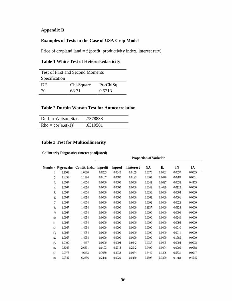
96

Appendix B

Examples of Tests in the Case of USA Crop Model

Price of cropland land = f (profit, productivity index, interest rate)

Table 1 White Test of Heteroskedasticity

Test of First and Second Moments

Specification

DF Chi-Square Pr>ChiSq

70 68.71 0.5213

Table 2 Durbin Watson Test for Autocorrelation

Durbin-Watson Stat. .7378838

Rho = cor[e,e(-1)] .6310581

Table 3 Test for Multicollinearity

Condit. Indx. lnprofit lnprod lninterest GA IL IN IA

1 2.1069 1.0000 0.0283 0.0345 0.0159 0.0070 0.0001 0.0037 0.0005

2 1.6259 1.1384 0.0107 0.0680 0.0123 0.0005 0.0070 0.0283 0.0001

3 1.0667 1.4054 0.0000 0.0000 0.0000 0.0041 0.0027 0.0033 0.4473

4 1.0667 1.4054 0.0000 0.0000 0.0000 0.0043 0.4099 0.0113 0.0000

5 1.0667 1.4054 0.0000 0.0000 0.0000 0.0056 0.0000 0.0004 0.0000

6 1.0667 1.4054 0.0000 0.0000 0.0000 0.0062 0.0000 0.0001 0.0000

7 1.0667 1.4054 0.0000 0.0000 0.0000 0.0002 0.0000 0.0023 0.0000

8 1.0667 1.4054 0.0000 0.0000 0.0000 0.3937 0.0000 0.0128 0.0000

9 1.0667 1.4054 0.0000 0.0000 0.0000 0.0000 0.0000 0.0006 0.0000

10 1.0667 1.4054 0.0000 0.0000 0.0000 0.0000 0.0000 0.0249 0.0000

11 1.0667 1.4054 0.0000 0.0000 0.0000 0.0000 0.0000 0.0095 0.0000

12 1.0667 1.4054 0.0000 0.0000 0.0000 0.0000 0.0000 0.0010 0.0000

13 1.0667 1.4054 0.0000 0.0000 0.0000 0.0000 0.0000 0.0011 0.0000

14 1.0667 1.4054 0.0000 0.0000 0.0000 0.0000 0.0000 0.1985 0.0000

15 1.0109 1.4437 0.0000 0.0004 0.6642 0.0037 0.0005 0.0004 0.0002

16 0.3046 2.6301 0.0103 0.5718 0.2542 0.0490 0.0004 0.0005 0.0088

17 0.0975 4.6493 0.7059 0.3233 0.0074 0.2449 0.1896 0.5531 0.0917

18 0.0542 6.2356 0.2448 0.0020 0.0460 0.2807 0.3899 0.1482 0.4515

Collinearity Diagnostics (intercept adjusted)

Number Eigenvalue

Proportion of Variation

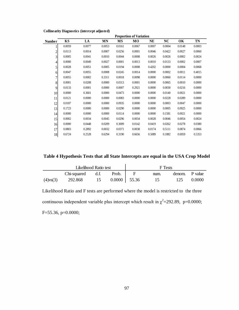
97

Table 4 Hypothesis Tests that all State Intercepts are equal in the USA Crop Model

Likelihood Ratio and F tests are performed where the model is restricted to the three

continuous independent variable plus intercept which result in χ2=292.89, p=0.0000;

F=55.36, p=0.0000;

KS LA MN MS MO NE NC OK TN

1 0.0059 0.0077 0.0053 0.0161 0.0067 0.0007 0.0004 0.0148 0.0003

2 0.0113 0.0014 0.0007 0.0256 0.0001 0.0046 0.0422 0.0027 0.0060

3 0.0005 0.0041 0.0010 0.0044 0.0008 0.0026 0.0026 0.0002 0.0024

4 0.0000 0.0049 0.0027 0.0001 0.0013 0.0010 0.0133 0.0002 0.0007

5 0.0028 0.0051 0.0005 0.0194 0.0008 0.4202 0.0000 0.0004 0.0068

6 0.0047 0.0055 0.0008 0.0245 0.0014 0.0000 0.0002 0.0011 0.4015

7 0.0055 0.0002 0.3311 0.0018 0.0098 0.0000 0.0060 0.0114 0.0000

8 0.0001 0.0208 0.0000 0.0313 0.0001 0.0000 0.0065 0.0010 0.0000

9 0.0133 0.0001 0.0000 0.0007 0.2921 0.0000 0.0030 0.0216 0.0000

10 0.0000 0.3601 0.0000 0.0473 0.0000 0.0000 0.0140 0.0021 0.0000

11 0.0121 0.0000 0.0000 0.0083 0.0000 0.0000 0.0228 0.0289 0.0000

12 0.0187 0.0000 0.0000 0.0935 0.0000 0.0000 0.0003 0.0047 0.0000

13 0.1723 0.0000 0.0000 0.0290 0.0000 0.0000 0.0005 0.0925 0.0000

14 0.0000 0.0000 0.0000 0.0114 0.0000 0.0000 0.1581 0.0021 0.0000

15 0.0002 0.0034 0.0045 0.0296 0.0034 0.0028 0.0046 0.0054 0.0024

16 0.0000 0.0448 0.0209 0.3009 0.0142 0.0419 0.0262 0.0278 0.0380

17 0.0803 0.2892 0.0032 0.0371 0.0038 0.0174 0.5111 0.0874 0.0066

18 0.6724 0.2528 0.6294 0.3190 0.6656 0.5089 0.1882 0.6959 0.5353


Number


Chi-squared d.f. Prob. F num. denom. P value

(4)vs(3) 292.868 15 0.0000 55.36 15 125 0.0000

Likelihood Ratio test F Tests

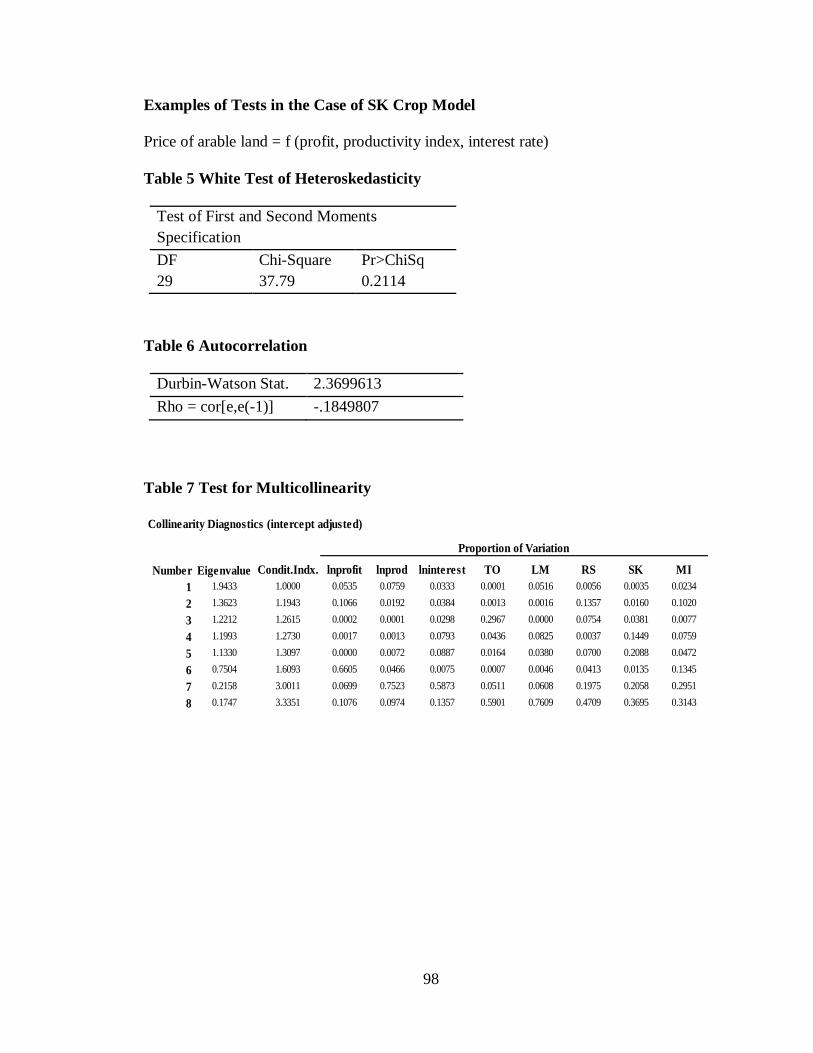
98

Examples of Tests in the Case of SK Crop Model

Price of arable land = f (profit, productivity index, interest rate)

Table 5 White Test of Heteroskedasticity

Test of First and Second Moments

Specification

DF Chi-Square Pr>ChiSq

29 37.79 0.2114

Table 6 Autocorrelation

Durbin-Watson Stat. 2.3699613

Rho = cor[e,e(-1)] -.1849807

Table 7 Test for Multicollinearity

Condit.Indx. lnprofit lnprod lninterest TO LM RS SK MI

1 1.9433 1.0000 0.0535 0.0759 0.0333 0.0001 0.0516 0.0056 0.0035 0.0234

2 1.3623 1.1943 0.1066 0.0192 0.0384 0.0013 0.0016 0.1357 0.0160 0.1020

3 1.2212 1.2615 0.0002 0.0001 0.0298 0.2967 0.0000 0.0754 0.0381 0.0077

4 1.1993 1.2730 0.0017 0.0013 0.0793 0.0436 0.0825 0.0037 0.1449 0.0759

5 1.1330 1.3097 0.0000 0.0072 0.0887 0.0164 0.0380 0.0700 0.2088 0.0472

6 0.7504 1.6093 0.6605 0.0466 0.0075 0.0007 0.0046 0.0413 0.0135 0.1345

7 0.2158 3.0011 0.0699 0.7523 0.5873 0.0511 0.0608 0.1975 0.2058 0.2951

8 0.1747 3.3351 0.1076 0.0974 0.1357 0.5901 0.7609 0.4709 0.3695 0.3143


Number Eigenvalue


99

Table 8 Hypothesis Tests that all the State Intercepts are equal in the SK Crop

Model

Likelihood Ratio and F tests are performed where the model is restricted to the three

continuous independent variables plus intercept which results in χ2=42.631, p=0.0000;

F=10.82, p=0.0000;

Table 9 Summary Statistics for Different Proxies of Profitability in USA Models

Output Price Index – the value is equal to 100 in the year 2000

Input Price Index- the value is equal to 100 in the year 1992

Chi-squared d.f Prob. F num denom P value

42.631 5 0.0000 10.82 5 45 0.0000

Likelihood Ratio test F test


Output Price Index 113.18 114.14 13.53 92.85 148.56 Input Price Index 129.66 120.79 18.41 92.22 163.66

Cash Rent ($/Ac) 226 185 76 63 408 Output Price Index 144.12 123.10 38.77 91.86 231.38 Input Price Index 151.89 146.00 24.47 125.00 193.00

Cash Rent ($/Ac) 21 16 10 6 41 Output Price Index 113.18 114.14 13.53 92.85 148.56 Input Price Index 120.78 124.00 12.32 102.00 138.00

Total

Crop

Animal

100

Models with Different Proxy for Profitability

Price of cropland = f (cash rent, productivity index, interest rate)

Table 10 USA Crop Model







R-squared 0.9224


Model test F [ 18, 125] (prob) 82.60(.0000)


LAGRENT 0.0154 0.0740 0.2070 0.8360 5.3248

LAGPROD 0.4526 0.1462 3.0960 0.0024 4.6987

LAGINTER -0.4114 0.1003 -4.1000 0.0001 1.4867

AR 5.6270 0.7435 7.5680 0.0000 0.0625

GA 6.3380 0.7402 8.5630 0.0000 0.0625

IL 6.5160 0.7256 8.9800 0.0000 0.0625

IN 6.4536 0.7301 8.8400 0.0000 0.0625

IA 6.3365 0.7308 8.6700 0.0000 0.0625

KS 5.1000 0.7214 7.0700 0.0000 0.0625

LA 5.6502 0.7402 7.6330 0.0000 0.0625

MN 6.0030 0.7141 8.4060 0.0000 0.0625

MS 5.5415 0.7564 7.3260 0.0000 0.0625

MO 5.9782 0.7145 8.3670 0.0000 0.0625

NE 5.6842 0.7359 7.7240 0.0000 0.0625

NC 6.5477 0.7205 9.0880 0.0000 0.0625

OK 5.1640 0.7076 7.2980 0.0000 0.0625

TN 6.2720 0.7351 8.5330 0.0000 0.0625

TX 5.3641 0.7376 7.2730 0.0000 0.0625

WI 6.3326 0.7113 8.9030 0.0000 0.0625

101

Price of pastureland = f (cash rent, productivity index, interest rate)

Table 11 USA Animal Model







R-squared 0.9040


Model test F [ 18, 125] (prob) 65.40(.0000)


LAGRENT -0.2971 0.2880 -1.0320 0.3042 2.9724

LAGPROD 0.5481 0.3409 1.6080 0.1104 4.6139

LAGINTER -0.8001 0.1477 -5.4190 0.0000 1.4867

AR 6.8765 1.8858 3.6460 0.0004 0.0625

GA 7.9898 1.9555 4.0860 0.0001 0.0625

IL 7.0408 2.0195 3.4860 0.0007 0.0625

IN 7.1817 2.0039 3.5840 0.0005 0.0625

IA 6.7954 2.0021 3.3940 0.0009 0.0625

KS 5.7029 1.8569 3.0710 0.0026 0.0625

LA 6.8783 1.9067 3.6070 0.0004 0.0625

MN 6.3468 1.9149 3.3140 0.0012 0.0625

MS 6.9043 1.8551 3.7220 0.0003 0.0625

MO 6.8033 1.9480 3.4920 0.0007 0.0625

NE 5.1646 1.8589 2.7780 0.0063 0.0625

NC 7.8144 1.9569 3.9930 0.0001 0.0625

OK 5.7731 1.7991 3.2090 0.0017 0.0625

TN 7.5132 1.9126 3.9280 0.0001 0.0625

TX 6.0330 1.7643 3.4200 0.0008 0.0625

WI 7.1005 2.0289 3.5000 0.0006 0.0625

102

Price of agricultural land = f (output price index, input price index, productivity index,

interest rate)

Table 12 USA Total Model







R-squared 0.9717


Model test F [ 18, 125] (prob) 224.83(.0000)


LAGOUT 0.4126 0.0921 4.4810 0.0000 4.7204

LAGINP 0.5931 0.0672 8.8200 0.0000 4.8014

LAGPROD -0.1866 0.0987 -1.8910 0.0609 4.6612

LAGINTER -0.1417 0.0692 -2.0490 0.0426 1.4867

AR 3.7286 0.5400 6.9050 0.0000 0.0625

GA 4.2446 0.5312 7.9910 0.0000 0.0625

IL 4.2380 0.5359 7.9080 0.0000 0.0625

IN 4.2161 0.5365 7.8590 0.0000 0.0625

IA 4.0695 0.5367 7.5830 0.0000 0.0625

KS 2.9385 0.5345 5.4970 0.0000 0.0625

LA 3.6743 0.5413 6.7870 0.0000 0.0625

MN 3.7861 0.5353 7.0730 0.0000 0.0625

MS 3.6622 0.5445 6.7260 0.0000 0.0625

MO 3.6876 0.5340 6.9060 0.0000 0.0625

NE 3.1036 0.5380 5.7680 0.0000 0.0625

NC 4.4642 0.5347 8.3500 0.0000 0.0625

OK 3.0255 0.5343 5.6620 0.0000 0.0625

TN 4.1890 0.5386 7.7770 0.0000 0.0625

TX 3.1899 0.5352 5.9600 0.0000 0.0625

WI 4.1152 0.5345 7.6990 0.0000 0.0625

103

Price of cropland = f (output price index, input price index, productivity index, interest

rate)

Table 13 USA Crop Model







R-squared 0.9767


Model test F [ 18, 125] (prob) 274.04(.0000)


LAGOUT 0.0041 0.0541 0.0760 0.9399 4.8617

LAGINP 0.9862 0.1041 9.4710 0.0000 4.9619

LAGPROD 0.1679 0.0781 2.1490 0.0336 4.6987

LAGINTER 0.1316 0.0628 2.0950 0.0382 1.4867

AR 1.3565 0.4781 2.8370 0.0053 0.0625

GA 2.0567 0.4786 4.2970 0.0000 0.0625

IL 2.2029 0.4707 4.6800 0.0000 0.0625

IN 2.1385 0.4694 4.5560 0.0000 0.0625

IA 2.0384 0.4734 4.3060 0.0000 0.0625

KS 0.7936 0.4736 1.6760 0.0963 0.0625

LA 1.3667 0.4758 2.8720 0.0048 0.0625

MN 1.6735 0.4691 3.5680 0.0005 0.0625

MS 1.3022 0.4839 2.6910 0.0081 0.0625

MO 1.6523 0.4701 3.5140 0.0006 0.0625

NE 1.4010 0.4762 2.9420 0.0039 0.0625

NC 2.2128 0.4681 4.7270 0.0000 0.0625

OK 0.8278 0.4693 1.7640 0.0802 0.0625

TN 1.9884 0.4772 4.1670 0.0001 0.0625

TX 1.0891 0.4795 2.2710 0.0248 0.0625

WI 1.9958 0.4679 4.2650 0.0000 0.0625

104

Price of pastureland = f (output price index, input price index, productivity index, interest

rate)

Table 14 USA Animal Model







R-squared 0.9664


Model test F [ 18, 125] (prob) 188.04(.0000)


LAGOUT 0.9092 0.1249 7.2790 0.0000 4.7204

LAGINP -1.1467 0.1435 -7.9900 0.0000 4.7937

LAGPROD 0.0035 0.2046 0.0170 0.9862 4.6139

LAGINTER -0.7533 0.1002 -7.5160 0.0000 1.4867

AR 9.6789 1.5488 6.2490 0.0000 0.0625

GA 10.6887 1.5581 6.8600 0.0000 0.0625

IL 9.6593 1.5604 6.1900 0.0000 0.0625

IN 9.8368 1.5671 6.2770 0.0000 0.0625

IA 9.3798 1.5499 6.0520 0.0000 0.0625

KS 8.5923 1.5519 5.5360 0.0000 0.0625

LA 9.6797 1.5570 6.2170 0.0000 0.0625

MN 9.0854 1.5563 5.8380 0.0000 0.0625

MS 9.6489 1.5387 6.2710 0.0000 0.0625

MO 9.4923 1.5509 6.1210 0.0000 0.0625

NE 8.1118 1.5584 5.2050 0.0000 0.0625

NC 10.5124 1.5586 6.7450 0.0000 0.0625

OK 8.7886 1.5532 5.6580 0.0000 0.0625

TN 10.2902 1.5552 6.6170 0.0000 0.0625

TX 9.0902 1.5505 5.8630 0.0000 0.0625

WI 9.6280 1.5583 6.1780 0.0000 0.0625

impact of agricultural profitability, productivity and

Documents