IMF Support and Inter-regime Exchange rate Volatility

Ivo J.M. Arnold∗ Universiteit Nyenrode, Breukelen, The Netherlands

Ronald MacDonald

University of Glasgow, Glasgow, United Kingdom

Casper G. de Vries Erasmus University Rotterdam and Tinbergen Institute

Rotterdam, The Netherlands

June 2007

Abstract

A widely held notion is that freely floating exchange rates are excessively volatile when moving from fixed to floating exchange rates. We re-examine the data and conclude that the disparity between the fundamentals and exchange rate volatility is more apparent than real, especially when the Deutsche Mark, rather than the dollar, is chosen as the numeraire currency. We argue and demonstrate that in inter-regime comparisons one has to account for certain ‘missing variables’ which compensate for the fundamental variables’ volatility under fixed exchange rates. We show that IMF credit support is a crucial compensating variable.

Keywords: Exchange rates; Exchange rate regimes; Excess volatility; IMF credit.

JEL classification: F31

∗ Contact details: Ivo J.M. Arnold, Universiteit Nyenrode, Straatweg 25, 3621 BG Breukelen, Netherlands (email: i.arnold@nyenrode.nl); Ronald MacDonald, Department of Economics, University of Glasgow, Adam Smith Building, Room S102, Glasgow G12 8RT, Scotland (email: r.macdonald@socsci.gla.ac.uk); Casper G. de Vries, Erasmus University Rotterdam, Tinbergen Institute, H14-25, PO Box 1738, 3000 DR Rotterdam, Netherlands (email: cdevries@few.eur.nl).

2

1. Introduction

The early proponents of flexible exchange rates (see, for example, Friedman, 1953, Sohmen, 1961 and Johnson, 1958) viewed the fixed but adjustable Bretton Woods exchange rate arrangement as inherently unstable, because it failed to provide an effective adjustment mechanism. In contrast, a regime of flexible exchange rates was regarded as providing an automatic adjustment mechanism and flexible rates were therefore predicted to be inherently stable. However, the post-Bretton Woods and inter-war experiences with flexible exchange rates suggest that exchange rates when left to their own devices are inherently volatile. Of course, this does not mean that such rates are excessively volatile, since as Friedman recognized, if the underlying fundamentals are unstable then exchange rates are likely to be unstable as well:

Instability of exchange rates is a symptom of instability in the underlying economic structure. Elimination of this symptom by administrative freezing of exchange rates cures none of the underlying difficulties and only makes adjustment to them more painful. (Friedman, 1953)

However, the so-called exchange rate disconnect discussed in Obstfeld and Rogoff (2000) summarizes a widely held belief in the profession that exchange rates have indeed been excessively volatile with respect to traditional macroeconomic variables in the post-Bretton Woods period.1 There are two aspects to this volatility disconnect in the literature, and we label these inter- and intra-regime volatility. Inter-regime volatility refers to the striking result that in moving from a system of fixed to floating exchange rates, the volatility of macroeconomic fundamentals, such as the money stock and income, does not change, but the volatility of the exchange rate does. The concept of intra-regime volatility refers to the view that in floating exchange rate regimes exchange rates appear to be excessively volatile with respect to the fundamentals. This paper focuses on the first issue of inter-regime volatility and leaves intra regime volatility to one side.

The issue of inter-regime volatility has been made in a number of papers. For example, Baxter and Stockman (1989) examine the variability of output, trade variables, private and government consumption and the real exchange rate and are “unable to find evidence that the cyclical behavior of real macroeconomic aggregates depends systematically on the exchange rate regime. The only exception is the well-known case of the real exchange rate.” Flood and Rose (1995) use flexible price and sticky price variants of the monetary model to show that the volatility of their so-called ‘traditional fundamentals’ (money and income) remains roughly unchanged in the move from the Bretton Woods to the post-Bretton Woods regime, but that the volatility of virtual fundamentals (the exchange rate minus the interest rate differential) increases dramatically. Flood and Rose (1999) present a similar exercise in which they compare the volatility of fundamentals (including the interest differential) with exchange rate volatility per se for the Bretton Woods and

1The exchange rate disconnect also refers to the apparent difficulty in forecasting (the level of) exchange rates, although this is not uncontroversial (see, for example, MacDonald (2007).

3

the post- Bretton Woods period and again find that the volatility of the exchange rate dominates the volatility of the fundamentals.2

In this paper we propose to re-evaluate the inter-regime volatility issue. On the theory side we expand the monetary model of floating exchange rates to account for ‘missing variables’ in the case of regulated markets. Since, for example, the Bretton Woods regime was characterized by fixed exchange rates combined with trade and capital market distortions, an analysis of this regime has to take account of such distortions.

A key novelty in our study lies in the examination of inter-regime volatility and, in particular, the behavior of an expanded set of fundamentals in the Bretton Woods and post-Bretton Woods periods. We shift the question from ‘why do we not observe more exchange rate volatility in fixed rate regimes given that standard fundamentals have similar volatility under both regimes?’ to ‘which variables absorb the fundamental volatility under fixed rates?’. We believe that asking the question in this way is insightful since there may be other fundamentals which absorbed the fundamentals’ variability in these regimes. If exchange rates are fixed, or managed, then it should be variables like trade restrictions, capital controls, international reserves or balance of payments support which adjust rather than the exchange rate. Marston (1993) showed, for example, that the interest differentials between the onshore and offshore Eurocurrency market under Bretton Woods was as large as one hundred basis points on an annual basis. Moreover, these differentials were highly variable. Furthermore, in these regimes there are often other regulatory aspects which should be incorporated into any empirical evaluation of the volatility of exchange rate fundamentals. We demonstrate that the volatility in the fundamentals is at least partly absorbed by these missing variables.

The outline of the remainder of this paper is as follows. In the next section we present an extension of the monetary model. This model is designed to motivate the kind of traditional fundamentals used in exchange rate studies and the incorporation of the distortionary variables or wedges. The extended model shows how volatility of the traditional fundamentals is absorbed by the wedges rather than the exchange rate. In section 3 we empirically investigate the inter-regime volatility. The last section concludes.

2Duarte (2003) examines the effects of the exchange rate regime in the context of a dynamic general equilibrium model with nominal goods prices set in the buyer’s currency and incomplete asset markets. Her model predicts a sharp increase in the volatility of the real exchange rate when moving from fixed to flexible exchange rates. This pattern is not observed for other variables. Reinhart and Rogoff (2002) argue that at least part of the inter-regime volatility puzzle may be explained by using an inappropriate classification of the exchange rate regime. In particular, they show that in moving from the IMF’s classification of an exchange rate regime (as used in the studies of Baxter and Stockman (1989) and Flood and Rose (1995, 1999)) to one based on the factual properties of the regime, there was in fact much more flexibility of exchange rates during Bretton Woods and much more rigidity during the post-Bretton Woods period.

4

2. Theoretical background

We adapt the standard flexible price monetary model to illustrate the relationship between fundamentals and the exchange rate. The incorporation of distortions drives a wedge between the exchange rate and the standard fundamentals. We go on to show how these may pick up the volatility in the fundamentals. We start with a modified version of absolute PPP:

*SPP Ω= . (2.1)

Here the domestic (traded goods) price deflator P equals the price of the consumption bundle in foreign (traded goods) prices P* times the distortion Ω and the exchange rate S. The distortion is responsible for the absence of absolute PPP (see Obstfeld and Rogoff (2000)) and signifies anything that drives or sustains a wedge between the domestic and foreign price levels. This includes tariff levies, export subsidies, transportation costs and the tariff equivalent of any quotas that drive a wedge between the foreign and domestic price levels. It also includes balance of payments support that is used to sustain current account deficits and postpone adjustment.

A more elaborate exchange rate model including standard macro variables is obtained by combining the PPP relation (2.1) with the domestic and foreign quantity theory based equations for money demand respectively:

φλ PYRM =)exp( and φλ )()exp( ∗∗∗∗ = YPRM . (2.2)

Taking the logarithm of (2.1) and substituting the home and foreign log transformed money demand functions gives the monetary model of the exchange rate:

ωλφ −+−= ryms . (2.3)

Here s = log(S) is the log exchange rate, m = log(M/M*) is the relative money supply, y = log(Y/Y*) is relative income, r = R-R* is the interest rate differential and ω = log(Ω) is the log of the wedge. Apart from the distortion,ω, the derivation gives the standard monetary approach exchange rate equation. More elaborate derivations based on individual agent optimization, as in Stockman (1980) and Lucas (1982), yield a pricing kernel. After calibration, the kernel reduces to specifications that are similar to (2.3) (see Mark (2001)). The specification (2.3) without the distortion matches the specification of the macro-economic fundamentals as in Flood and Rose (1999, p. 663). Omitting λr-ω from (2.3) gives the so-called traditional fundamental from Flood and Rose (1995).

Note that the wedge in (2.3) enters with a negative sign, as in the case of relative incomes, since it keeps domestic prices artificially higher than the foreign prices thereby improving the terms of trade. If the wedge adjusts to counter the movements in the traditional fundamentals, it can compensate for the fluctuations in these other driving factors. How can we ensure that ω is chosen correctly? Some of the distortions to free trade, like the costs of transportation, can hardly react to changes in the fundamentals. But other distortions like the implicit price distortions induced by a quota or variable balance of payments support, and interest rate differentials, as the result of capital controls and official reserves or IMF credit, may be sufficiently flexible to absorb

5

the fundamentals’ movements and keep the spot rate constant. The case of Germany in the 1960’s and more recently the case of China shows that massive reserve hoarding, in combination with inward capital controls, can for extended periods of time take away the pressure for appreciation. While more difficult in the other direction due to limited means, devaluation has been postponed by employing reserves or foreign credit. To make a link to the empirical section, we compute the variance on both sides of the exchange rate equation (2.3):

.222222 ,,,,,,22222

ωωωω σσσσσσσσσσσ ryrymrmymryms −+−−+−+++= (2.4)

On the one hand, under a free float without movements in the wedge, the volatility equation reduces to:

.222 ,,,2222

ryrmymryms σσσσσσσ −+−++= (2.5)

In a fixed exchange rate regime on the other hand, (2.4) becomes:

.2222220 ,,,,,,2222

ωωωω σσσσσσσσσσ ryrymrmymrym −+−−+−+++= (2.6)

The received evidence is that there is little or no difference in the variability of the traditional fundamentals across regimes. If this is the case, equations (2.5) and (2.6) show that

ωωωω σσσσ ,,,2 222 rym −+− , (2.7)

has to bear the brunt of foreign exchange rate stabilization. These variance and covariance terms related to the wedge need to compensate for the volatility in the fundamentals in such a way that the exchange rate variability, σs

2, is nil. Under a dirty float, all terms in (2.4) will in general be non-zero. The next section tries to identify the missing variances and covariances in (2.7).

3. Inter-regime volatility

In this section we combine data from the Bretton Woods and post-Bretton Woods periods to address the issue of the importance of the wedge in explaining why traditional monetary fundamentals may not be enough to explain inter-regime volatility. As cross-country data on tariffs and subsidies are not widely available, we focus on balance of payments support as an important factor in postponing exchange rate adjustment.

We start by examining the role of IMF support in suppressing exchange rate variability during the Bretton Woods period. We then go on to combine IMF support with traditional fundamentals, like money and income, to address the volatility issue. The volatility comparisons will be done using both annual and monthly datasets. Both datasets span the Bretton Woods and post-Bretton Woods periods and for European currencies include the period in which the ERM operated. This variation in regimes within the dataset follows Flood and Rose (1995) and is essential for an empirical investigation of inter-regime volatility. Throughout the empirical analysis, two countries will be used as numeraire: the United States (1) and Germany (2). Although the US was clearly the dominant numeraire currency in the Bretton Woods period, Germany’s importance increased in the post-Bretton Woods period, particularly after the formation of the ERM.

6

To the extent that central banks use foreign exchange reserves to stabilize the exchange rate, a tradeoff between exchange rate and reserve volatility would be expected. According to the monetary approach to the balance of payments, a divergence in the fundamentals (e.g. high domestic money growth) must be dissipated through a loss of reserves or the peg will have to be abandoned. Note, however, that we do not expect such a trade-off when the fundamentals do not diverge.

There appears to be little in the way of empirical evidence supporting a trade-off between exchange rate and reserve volatility. Intuitively, the abandonment of a peg would be expected to lead to a reduction in reserve holdings and their volatility. However, Flood and Rose (1995) find that the volatility of reserves is generally higher following the collapse of the Bretton Woods system. We offer an explanation for this apparent absence of a tradeoff. A key reason why there may not be a stronger trade-off between reserves and exchange rate volatility is because IMF credit facilities distort the relationship. As IMF credit has often been used to replenish a country’s dwindling reserves, it masks the visibility of balance of payments problems in data on reserves. We therefore argue that any analysis of the trade-off between exchange rate and reserve volatility needs to take into account the role of IMF credit in supporting weak currencies.

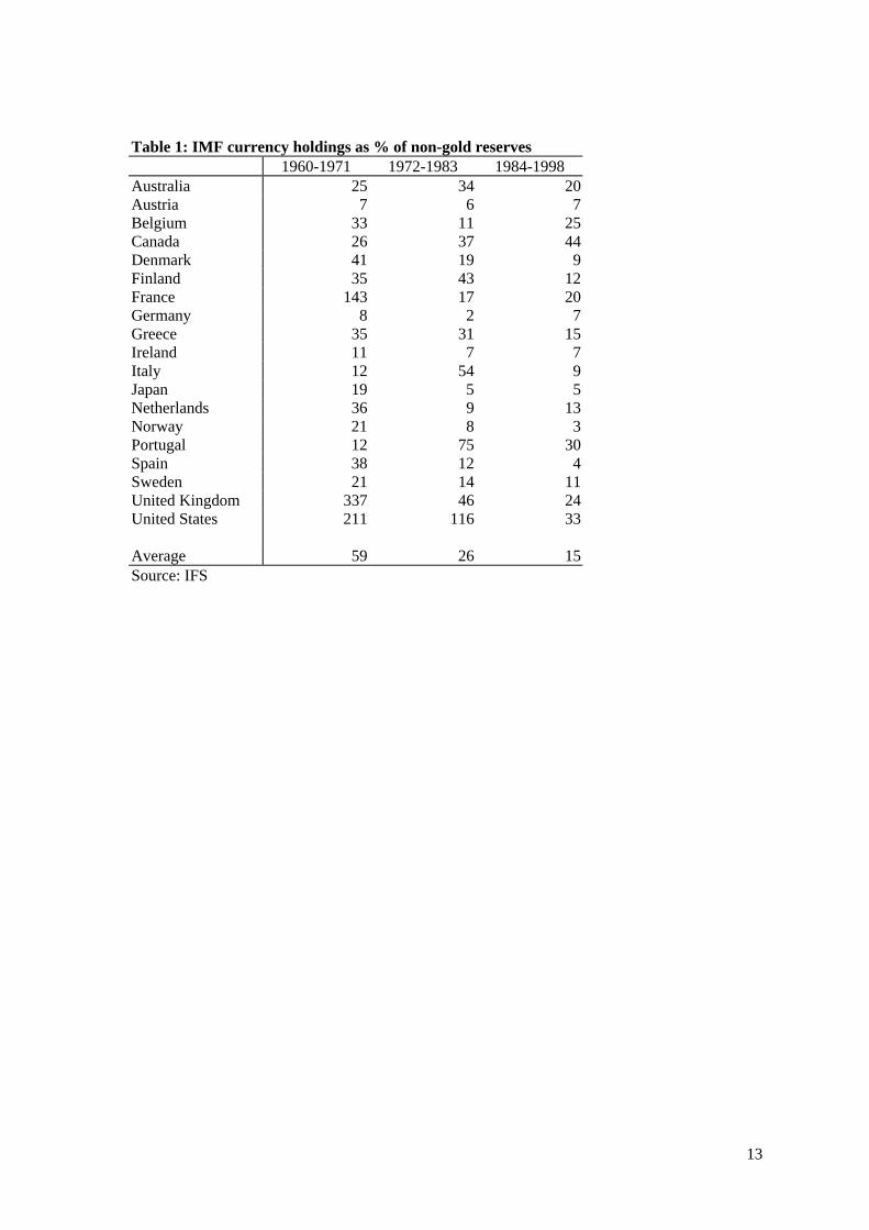
We first investigate whether IMF support is quantitatively sufficiently important to be included in an analysis of the volatility tradeoff. Table 1 shows the IMF's holdings of currency as a percentage of non-gold reserves for all countries during three subperiods. In general this percentage is highest during the Bretton Woods years and in the 1970s. With a few exceptions the percentage has declined from the 1980s onwards.3 In the remainder of our analysis we look at the IMF holdings of a currency as a percentage of its IMF quota, to correct for the effect of quota increases. In their analyses of the volatility trade-off, Flood and Rose (1995) examined if the existence of non-gold reserves was an important source of fundamental volatility. They concluded it was not. Our discussion here suggests that it is not sufficient to rely on non-gold reserves, rather Fund credit or Fund holdings of currency should be taken into consideration. We thus opt for Fund holdings of currency as a percentage of Fund quota and refer to this as our IMF variable.

Figure 1 contains scatter plots of the change in the exchange rate (against the dollar, in dlog) versus, respectively, the change in our IMF variable (in dlog) in the top plot and the change in non-gold reserves (in dlog) in the bottom plot. The data are monthly and combine the experiences of 21 countries over the period 1960 to 1998 (see the data appendix for a list of countries). Figures 2 and 3 report some individual countries experiences. The scatter-plot for the IMF variable is shaped in the form of a cross, implying a highly non-linear dependence between changes in the exchange rate and the IMF measure. There thus exists a volatility tradeoff, though not a linear one. Either exchange rates or the Fund holdings of a currency are adjusting, but hardly ever are the two mechanisms for adjustment combined. In comparison, the scatter-plot for non-gold reserves has much less observations along the axes, suggesting the absence of a similar

3 In Table 1, the high percentage for France during the first sub-period can be partly explained by the fact that France had chosen to hold most of its reserves in gold instead of in foreign currency.

7

non-linear tradeoff between changes in the exchange rate and non-gold reserves. Here the two adjustment mechanisms are repeatedly used in tandem, or even occur in such a way that one partly compensates the other. This suggests that non-gold reserves and foreign exchange adjustments mostly acted in a complementary manner, while IMF credit was an almost perfect substitute for exchange rate movements. This conclusion is only reinforced by the per country graphs in the Appendix. Based on the magnitude of IMF support (especially in the Bretton Woods period) and the cross-shaped pattern in the top plot of Figure 1, we have chosen the IMF variable as our candidate measure of the wedge ω . In the next two sections, we combine the IMF variable with traditional fundamentals to estimate

3.1 Volatility comparisons: annual data

An initial pass at the issue of inter-regime volatility by means of equations (2.5)-(2.7) we present in Table 2 the variances of two traditional macroeconomic fundamentals, namely the annual inflation and income growth differentials, along with the change in the exchange rate and the change in our IMF support variable across 19 countries (see Table A1 in the data appendix for a listing of countries). The use of annual data has the advantage of reducing short-term noise in the macroeconomic data while preserving the underlying signal. As this comes at the cost of a reduction in the number of observations, an analysis of monthly data is added in the next subsection. In the empirical analysis we have chosen inflation instead of money supply growth as our monetary fundamental because of the limited availability of money growth data for several countries in the 1960s. This is an important consideration in view of the small sample size of our annual analysis. We will redress this in the monthly analysis below, which includes money growth. The variances in Table 2 have the US and Germany as their numeraire countries and are calculated for three subperiods of comparable length (a Bretton Woods period, from 1961 to 1971, and two post Bretton Woods periods, respectively from 1972 to 1983 and from 1984 to 1998). Not only are these periods of equal length, but they also cover more or less the three regimes that prevailed: fixed exchange rates with adjustable peg supported by current and capital account restrictions and IMF credit, floating exchange rates but retaining balance of payment restrictions, capital controls and IMF support, and a complete free float.

The first point to note from these results is that they confirm the point made by a number of other researchers, that in moving from Bretton Woods to the post-Bretton Woods period the volatility of standard fundamentals is very similar but the volatility of the exchange rate increases substantially. Note, however, that in the floating periods exchange rate volatility vis-à-vis the dollar is almost twice the volatility vis-à-vis the DM. This suggests that the volatility issue might be at least partly a dollar issue. We will return to this theme below. The results in Table 2 also indicate that there is a lot of volatility stemming from the IMF variable in the Bretton Woods period and, interestingly, that the average volatility of this variable decreases as we move into the first post-Bretton Woods period and decreases substantially in the period when capital controls were finally relaxed (1984-1998). There thus appears to be a clear trade-off between exchange rate volatility and volatility in IMF support as one moves between the regimes.

8

To explicate the inter-regime volatility we run regressions of exchange rate volatility on fundamental volatility as specified in equation (2.4). As we noted, under a fixed regime (2.4) collapses to (2.6) while in a undistorted free float (2.4) reduces to (2.5). If one has only data from these two pure regimes, a regression of σs

2 on fundamentals σm2, σy

2, σr2 and the wedge σω

2, should give a negative coefficient on the latter variable. The intuition for this is in Figure 1. Since under a pure float σs

2=0 and in a undistorted free float σω2=0, the variances in both cases lie on a

hyperplane of a dimension lower than if all variances are non-zero. One can show that this implies a negative sign on the σω

2 variable in a regression of exchange rate volatility on the volatilities of the fundamentals and the wedge.4 Since a fair number of observations comes from the dirty float period in the 1970s and we have ommitted variables, we do not expect a perfect correspondence between the theoretical specification in (2.4) and the empirical results.

In Table 3 we estimate equation (2.4) using the annual dataset by means of generalized least squares on the panel of 19 countries and for the 3 subperiods identified above. This yields a total of 57 observations. For both numeraire currencies, we report three different specifications, which differ depending on the inclusion of covariance terms and the IMF variable. Interest rates have been omitted from the regressions due to lack of data. Below, we will include interest rates in a smaller sample of monthly data. Table 3 yields some interesting observations. First, the explanatory power of the DM regressions is high compared to the results for the dollar. Whereas fundamentals explain over 50% of the variance of the exchange rate vis-à-vis the German currency, the explanatory power versus the dollar sticks at around 25%. The second observation relates to the sign and significance of the traditional fundamentals. For the German numeraire, the variances of inflation and income growth are positively and significantly related to the variance of the exchange rate, as one would expect from the monetary model. Together these two variances can explain 56% of the variance in the DM exchange rate. Inflation and income growth do much worse in the dollar regressions, where the variance of inflation is barely significant and the variance of income has the wrong sign.

Turning to the variance and covariances involving the IMF variable, we observe that these are highly significant in the dollar regressions, but less so in the DM regressions. In all specifications, the variance of the IMF variable has a negative sign, as explained above. This corresponds to the visual impression from Figure 1, which illustrated the negative cross-shaped dependence between the exchange rate and IMF support, and also makes intuitive sense, as fluctuations in IMF support might serve to stabilize the currency.

According to (2.4), volatility in IMF support should increase exchange rate volatility, ceteris paribus the volatility in other fundamental variables. It is only by covarying with the traditional fundamentals that IMF support should result in lower exchange rate volatility. A good example of how this works is the negative and significant coefficient of covar(Δp, ΔIMF) in the dollar specification. This can be interpreted quite easily: inflationary policies in the Bretton Woods period could be sustained longer without the need for an exchange rate adjustment when IMF

4 In regression terms, this is due to zeros in the X-matrix with the explanatory variables, and zeros in the y-vector with the dependent variable in particular places.

9

support was made available. A positive covariance between Δp and ΔIMF thus reduces var(Δs). The negative sign of the coefficient of var(ΔIMF) has been explained in regression terms above. In addition, inflation and income may inadequately capture fundamental volatility. The significant negative sign for var(ΔIMF) may then pick up the covariances between IMF support and other missing fundamental variables. Candidates for such missing variables are, for example, fiscal policy variables and the current account.

Summarizing our annual results, we conclude that the extent to which the volatility issue is a puzzle seems to depend on the choice of numeraire. The traditional fundamentals do well in the DM regressions, but badly in the dollar regressions. In addition, our IMF variable adds explanatory power to both the dollar and DM regressions. We will now investigate whether these results are upheld using a monthly dataset.

3.2 Volatility comparisons: monthly data

We use monthly data to derive annual standard deviations (based on 12 non-overlapping monthly observations) as our volatility measures. These are calculated only for complete years (i.e. years for which we have 12 monthly observations). In principle, this yields 39 (years) times 21 (countries) = 819 observations, but in practice limited data availability reduced this number, see the bottom line of Table 4. For all variables, except IMF support, we take the first differences of the logs relative to the numeraire. See the data appendix for full details.

Table 4 reports regression results for a large sample including all countries except Switzerland (for which the IMF measure was unavailable for most of the sample period). Due to the limited data availability for many countries, this regression again excludes interest rate volatility, but we can now use money growth instead of inflation. Table 4 shows that the variance of money growth is significantly related to exchange rate volatility in all specifications. Income volatility is unrelated to exchange rate volatility in all regressions. Similar to the annual results, the volatility connection holds better versus Germany than versus the US, both in terms of significance and explanatory power. For both numeraires, the coefficient of covar(Δm, ΔIMF) is significantly negative, implying that IMF support can reduce or postpone the spill-over of a relatively high money growth into exchange rate volatility. This result resembles the significance of covar(Δp, ΔIMF) in the annual dollar regressions. It supports our interpretation of IMF support as driving a wedge between the volatility in traditional fundamentals and exchange rate volatility. In addition to the covariance term, var(ΔIMF) is significantly negative in the DM regressions. This also corresponds to the annual results; see the previous section for explanations for the negative sign of the coefficient of var(ΔIMF). A rerun of these regressions in which IMF support is replaced by non-gold reserves yields insignificant coefficients on the reserves variables, confirming the results of Flood and Rose (1995).

In order to ensure that our regression results do not depend on the inclusion of small high-inflation countries, Table 5 reports the results of a balanced panel regression for six large industrialized countries (Canada, France, Italy, Australia, the UK and either the US or Germany). Note that the number of observations is much lower than in the full monthly dataset. This set of

10

results shows the starkest contrast between the two numeraires. While the dollar regressions fail overall to establish a link between fundamental volatility and exchange rate volatility (except for the covariance term between money and income growth), the DM regressions are much stronger. All variances except var(Δy) are significantly related to var(Δs), including the variance of the long-term interest rate (var(Δil)).5 In addition, three out of six covariance terms are significant at at least a 10% level. Given the self-imposed constraint of a cross-section limited to just six countries, this is a strong result.

We conclude that the monthly data confirm the annual results. The fundamental connection is strongest in regressions which take the DM as the numeraire currency. In the majority of the regressions, there also appears to be a role for IMF support in explaining the wedge between fundamental and exchange rate volatility. That said, the explanation of currency volatility vis-à-vis the dollar remains a challenge, although on the basis of our discussion in Section 2, access to a broader range of distortionary variables would likely help in explaining this volatility.

4. Conclusions

There exists a widely held notion that freely floating exchange rates become excessively volatile when moving from fixed to floating exchange rates. This paper reexamines the issue of inter-regime volatility. We confirm the findings of a number of other researchers that in moving from fixed to floating exchange rates the variability of the standard macroeconomic fundamentals stays roughly unchanged, but that the volatility of the exchange rate changes considerably, suggesting an apparent mismatch. Using a simple extended version of the monetary model, we have demonstrated the importance of distortions in potentially explaining this mismatch and, specifically, how the volatility of standard fundamentals gets absorbed in fixed exchange rate regimes. In particular, we have shown that a country’s position at the IMF is an important source of compensating volatility, i.e. in suppressing volatility. Other distortions are also likely to be important in this regard, although unfortunately empirical data on these is limited or non-existent. In sum, we argue, and indeed demonstrate, that in cross-regime comparisons one has to account for the missing variables which compensate for the fundamental variables volatility under fixed rates. Moreover, we find that the volatility issue may be partly a dollar issue, as the link between fundamental volatility and exchange rate volatility improves markedly if we switch the numeraire from the dollar to the DM.

5 The long-term interest rate did somewhat better in these regressions than the short-term interest rate.

11

References

Baxter, M. and A. Stockman (1989), Business cycles and the exchange rate regime: some international evidence, Journal of Monetary Economics, 23, 3, 377-400.

Duarte, M. (2003), Why don't macroeconomic quantities respond to exchange rate variability, Journal of Monetary Economics, 50, 889-913.

Flood, R. and A. Rose (1995), Fixing exchange rates: a virtual quest for fundamentals, Journal of Monetary Economics, 36, 3-37.

Flood, R. and A. Rose (1999), Understanding exchange rate volatility without the contrivance of fundamentals, Economic Journal, 109, 660-672.

Friedman, M. (1953), The case for flexible exchange rates, in: Essays in positive economics, Chicago: Chicago University Press, 157-203.

Johnson, H.G. (1958), International trade and economic growth, Cambridge Mass: Harvard University Press.

Lucas Jr., R.E. (1982), Interest rates and currency prices in a two-country world, Journal of Monetary Economics 10, 335-359.

MacDonald, R. (2007), Exchange Rate Economics: Theories and Evidence, Taylor and Francis Mark, N.C. (2001), International Macroeconomics and Finance: Theory and Econometric Methods, Blackwell Publishers.

Marston, R.C. (1993), Interest differentials under Bretton Woods and the post-Bretton Woods float: The effects of capital controls and exchange risk, in A Retrospective on the Bretton Woods System, by M.D. Bordo and B. Eichengreen eds, NBER, The University of Chicago press, Chicago, 515-538

Obstfeld, M. and K. Rogoff (2000), The six major puzzles in international macroeconomics: is there a common cause?, in: B. Bernanke and K. Rogoff (eds), NBER Macroeconomics Annual, Cambridge: MIT Press, 339-390.

Reinhart, C.M. and K. Rogoff (2002), The modern history of exchange rate arrangements: a reinterpretation’, NBER working paper 8963.

Sohmen, E. (1961), Flexible exchange rates, Chicago: Chicago University Press.

Stockman, A.C. (1980) A theory of exchange rate determination, Journal of Political Economy 88, 673-698.

12

Data appendix

The annual macro-economic data have been taken from the European Commission AMECO database, except the data on IMF support, which have been derived using data from the IFS cd-rom (see below). The following countries are included: Australia, Austria, Belgium, Canada, Denmark, Finland, France, Germany, Greece, Ireland, Italy, Japan, Netherlands, New Zealand, Norway, Portugal, Spain, Sweden, United Kingdom and the USA.

The monthly macro-economic data have been taken from the IFS cd-rom. The data are monthly and start in January 1960. Due to the introduction of the euro in January 1999, the sample period ends in December 1998. The following countries are included: Australia, Austria, Belgium, Canada, Denmark, Finland, France, Germany, Greece, Ireland, Italy, Japan, Korea, Netherlands, Norway, Portugal, South-Africa, Spain, Sweden, Switzerland, United Kingdom and the USA. Our exchange rate measure is the bilateral period-average price of the US\ dollar (IFS line rf). We choose M1 (IFS line 34 or national definition) as our monetary aggregate. Where M1 was not available, we have chosen either a narrower (currency, IFS line 34A) or a broader aggregate (IFS line 35M or the national definition). To control for seasonality, we filter the money series by applying a one-sided moving average of the current observation and 12-lagged values (cf. Mark and Sul, 2001). The seasonally adjusted industrial production index (IFS line 66) is used for output; the CPI (IFS line 64) for prices. We use both long-term (IFS line 61) and short-term interest rates (IFS lines 60b/60c). Off-shore interest rates are available for a only few countries. Regarding reserves, we use non-gold reserves (IFS line 1L) and Fund holdings of domestic currency as a percentage of quota (IFS line 2F). The latter measure - denoted IMF - indicates the extent to which a country draws upon the IMF. Data on the exchange rate and non-gold reserves are available for all countries over the complete sample period. The same applies to the IMF measure, with the exception of Portugal (1962:7-1998:12) and Switzerland (1992:2-1998:12). The availability of other series is indicated in Table A1. All data have been checked and corrected for errors. With the exception of interest rates, the data are transformed by natural logarithms. Interest rates are measured as nominal rates divided by 1200.

13

Table 1: IMF currency holdings as % of non-gold reserves 1960-1971 1972-1983 1984-1998 Australia 25 34 20Austria 7 6 7Belgium 33 11 25Canada 26 37 44Denmark 41 19 9Finland 35 43 12France 143 17 20Germany 8 2 7Greece 35 31 15Ireland 11 7 7Italy 12 54 9Japan 19 5 5Netherlands 36 9 13Norway 21 8 3Portugal 12 75 30Spain 38 12 4Sweden 21 14 11United Kingdom 337 46 24United States 211 116 33 Average 59 26 15Source: IFS

14

Table 2: Volatility comparisons: average variances for 19 countries based on annual data

BW Post-BW I Post BW II 1961-1971 1972-1983 1984-1998

$ numeraire var(Δp) 4.6 10.6 5.9var(Δy) 8.5 8.4 4.7var(Δs) 8.1 111.7 117.6var(ΔIMF) (/100) 36.8 19.9 2.5 DM numeraire var( pΔ ) 5.2 11.5 8.0var( yΔ ) 6.3 5.4 6.4var( sΔ ) 11.7 56.0 59.3var( IMFΔ ) (/100) 32.8 15.3 2.5Data source: European Commision and IFS. Variances are computed from 100*dlog x, where x is the variable under consideration.

Table 3: Panel regressions: annual data var(Δs) vs $ vs $ vs $ vs DM vs DM vs DM constant 69.78 85.66 71.38 6.76 13.59 9.53 (2.86) (3.79) (2.49) (1.20) (3.09) (2.31) var(Δp) 3.13* 2.79 4.47* 2.03** 1.85** 3.06** (1.79) (1.44) (1.87) (9.40) (14.08) (7.31) var(Δy) -3.53** -3.87** -1.43** 1.54** 1.35** 0.58* (3.26) (2.69) (2.42) (3.28) (5.97) (1.67) var(ΔIMF) -0.004** -0.005** -0.002** -0.0012 (3.85) (4.30) (4.73) (1.25) covar(Δp, Δy) 7.01** 2.85** (2.85) (4.22) covar(Δp, ΔIMF) -0.42** -0.036 (12.24) (0.24) covar(Δy, ΔIMF) -0.08 -0.031 (0.45) (0.35) # observations 57 57 57 57 57 57 weighted adj. R2 0.24 0.24 0.27 0.56 0.65 0.61 GLS estimation with cross-section weights, t-stats in parentheses are calculated using white cross-section standard errors. Balanced panel of 19 countries; variances and covariances calculated using annual data for three subperiods (1961-1971; 1972-1983; 1984-1998); * and ** indicate significance at respectively 10% and 5% levels.

15

Table 4: Panel regressions: monthly data, full sample vs $ vs $ vs $ vs DM vs DM vs DM

constant 0.0004 0.0004 0.0004 0.0005 0.0005 0.0005 (7.64) (7.83) (7.61) (7.98) (8.30) (7.94) var(Δm) 8.27** 8.21** 8.36** 21.90** 21.69** 21.02** (2.41) (2.38) (2.50) (3.81) (3.67) (3.75) var(Δy) -0.005 -0.003 0.002 0.013 0.016 0.022 (0.78) (0.40) (0.29) (0.68) (0.95) (1.21) var(ΔIMF) -0.0007 -0.0007 -0.002** -0.001** (0.83) (1.03) (3.37) (2.00) covar(Δm,Δy) -0.078 0.886 (0.07) (0.62) covar(Δm,ΔIMF) -0.976** -1.653** (2.45) (4.15) covar(Δy,ΔIMF) -0.02 -0.016 (1.58) (0.76) # observations 680 680 680 672 672 672 weighted adj. R2 -0.013 -0.018 -0.010 0.09 0.11 0.12 GLS estimation with cross-section weights, t-stats in parentheses are calculated using white cross-section standard errors. Unbalanced panel of 20 countries; annual variances and covariances calculated using monthly data from 1960.01 to 1998.12; * and ** indicate significance at respec-tively 10% and 5% levels.

16

Table 5: Panel regressions: monthly data, small sample vs $ vs $ vs $ vs DM vs DM vs DM

constant 0.0004 0.0004 0.0003 0.0004 0.0004 0.0004 (5.44) (5.62) (5.83) (5.50) (5.75) (4.86) var(Δm) 2.45 3.71 4.33 17.75** 18.64** 20.56** (0.49) (0.73) (0.94) (2.05) (2.09) (2.39) var(Δy) -0.010 -0.007 0.136* -0.029** -0.012 0.023 (0.85) (0.47) (1.83) (3.22) (0.96) (0.34) var(Δil) 2.12 2.50 2.40 8.79** 8.37** 7.11** (0.80) (0.95) (0.95) (3.28) (3.31) (3.30) var(ΔIMF) -0.000 -0.000 -0.003** -0.003** (0.93) (0.00) (2.75) (3.47) covar(Δm,Δy) 14.02** -0.358 (2.59) (0.08) covar(Δm,Δil) -21.29 35.88* (1.43) (1.84) covar(Δm,ΔIMF) -0.486 -1.60* (0.87) (1.70) covar(Δy,Δil) -1.877 4.49** (1.06) (2.03) covar(Δy,ΔIMF) -0.086 -0.001 (1.36) (0.02) covar(Δil,ΔIMF) -0.902 -0.654 (1.18) (1.02) # observations 216 216 216 216 216 216 Weighted adj. R2 -0.13 -0.13 -0.10 0.06 0.07 0.12 GLS estimation with cross-section weights, t-stats in parentheses are calculated using white cross-section standard errors. Balanced panel of 6 countries (Canada, France, Italy, UK, Australia and either the US or Germany); annual variances and covariances calculated using monthly data from 1963.01 to 1998.12; * and ** indicate significance at respectively 10% and 5% levels.

17

Table A1: Data availability, monthly dataset M Y P il

Australia 60:1-98:12 M1 60:1-98:12 60:2-98:123 60:1-98:12 Austria 60:1-98:10 M1 60:1-98:12 60:1-98:12 71:1-98:12 Belgium 64:1-98:12 M11 60:1-98:12 60:1-98:12 63:9-98:12 Canada 60:1-98:12 M1 60:1-98:12 60:1-98:12 60:1-98:12 Denmark 60:1-98:12 M1 74:1-98:12 67:1-98:12 60:1-98:12 Finland 69:1-98:12 Currency 60:1-98:12 60:1-98:12 92:11-98:12 France 60:1-98:12 M1 60:1-98:12 60:1-98:12 60:1-98:12 Germany 61:1-98:12 M1 60:1-98:12 60:1-98:12 60:1-98:12 Greece 68:12-98:12 Currency 60:1-98:12 60:1-98:12 86:5-88:12 97:5-98:12 Ireland 67:1-98:12 Currency 60:1-98:12 60:2-98:123 64:1-98:12 Italy 62:1-98:12 M1 60:1-98:12 60:1-98:12 60:1-98:12 Japan 63:1-98:12 M1 60:1-98:12 60:1-98:12 66:11-98:12 Korea 60:1-98:12 M1 60:1-98:12 70:1-98:12 73:5-98:12 Netherlands 60:1-97:12 M1 60:1-98:12 60:1-98:12 64:11-98:12 Norway 60:1-98:12 Broad M 60:1-98:12 60:1-98:12 61:9-80:7 80:10-98:12 Portugal 76:1-98:12 Currency 60:1-98:12 60:1-98:12 60:1-64:4 76:1-98:12 South-Africa 60:1-91:6 M1 61:1-98:12 60:1-98:12 60:1-98:12 92:1-98:12 Spain 62:1-98:12 M1 61:1-98:12 60:1-98:12 78:3-98:12 Sweden 61:1-98:12 Broad M 60:1-98:12 60:1-98:12 60:1-95:12 Switzerland 60:1-98:12 M1 63:2-98:12 60:1-98:12 64:1-98:12 UK 60:1-98:12 M02 60:1-98:12 60:1-98:12 60:1-98:12 US 60:1-98:12 M1 60:1-98:12 60:1-98:12 60:1-98:12 1Currency (line 34a) until 79:12, thereafter M1. Ratio-spliced. 2Broad money (line 35L) until 75:5, thereafter M0. Ratio-spliced. 3Interpolated from quarterly data.

18

Figures

Figure 1: The cross (1960-1998)

-2

-1.5

-1

-0.5

0

0.5

1

1.5

2

-0.2 -0.15 -0.1 -0.05 0 0.05 0.1 0.15 0.2

Exchange rate vs $ (in dlog)

IMF

(in d

log)

-2

-1.5

-1

-0.5

0

0.5

1

1.5

2

-0.2 -0.15 -0.1 -0.05 0 0.05 0.1 0.15 0.2

Exchange rate vs $ (in dlog)

Non

-gol

d re

serv

es (i

n dl

og)

19

-2

-1

0

1

2

-.2 -.1 .0 .1 .2

Exchange rate vs $ (in dlog)

IMF

(in d

log)

-2

-1

0

1

2

-.2 -.1 .0 .1 .2

Exchange rate vs $ (in dlog)

Non

-gol

d re

serv

es (i

n dl

og)

20

Figure 2: % Change in IMF holdings of currency (hor. axis) vs % change in dollar exchange rate (vert. axis), 1960-1998

-.08

-.04

.00

.04

.08

.12

.16

-.6 -.4 -.2 .0 .2 .4 .6

Australia

-.15

-.10

-.05

.00

.05

.10

.15

-1.2 -0.8 -0.4 0.0 0.4 0.8 1.2

Belgium

-.04

-.03

-.02

-.01

.00

.01

.02

.03

.04

.05

-.4 -.2 .0 .2 .4 .6 .8

Canada

-.08

-.04

.00

.04

.08

.12

-.6 -.4 -.2 .0 .2 .4 .6

Denmark

-.08

-.04

.00

.04

.08

.12

.16

.20

.24

.28

-.4 -.2 .0 .2 .4 .6 .8

Finland

-.12

-.08

-.04

.00

.04

.08

.12

.16

-0.5 0.0 0.5 1.0 1.5

France

-.12

-.08

-.04

.00

.04

.08

.12

-3 -2 -1 0 1 2 3

Germany

-.08

-.04

.00

.04

.08

.12

.16

-.2 -.1 .0 .1 .2 .3

Greece

-.08

-.04

.00

.04

.08

.12

.16

-.6 -.4 -.2 .0 .2 .4 .6 .8

Ireland

-.15

-.10

-.05

.00

.05

.10

.15

-3 -2 -1 0 1 2

Italy

-.16

-.12

-.08

-.04

.00

.04

.08

.12

-1.2 -0.8 -0.4 0.0 0.4 0.8

Japan

-.1

.0

.1

.2

.3

.4

.5

.6

.7

-1 0 1 2 3 4

Korea

-.12

-.08

-.04

.00

.04

.08

.12

-1.5 -1.0 -0.5 0.0 0.5 1.0

Netherlands

-.08

-.06

-.04

-.02

.00

.02

.04

.06

.08

-.6 -.4 -.2 .0 .2 .4 .6 .8

Norway

-.12

-.08

-.04

.00

.04

.08

.12

-3 -2 -1 0 1 2 3

Austria

-.08

-.04

.00

.04

.08

.12

.16

.20

-0.8 -0.4 0.0 0.4 0.8 1.2

Portugal

-.15

-.10

-.05

.00

.05

.10

.15

.20

-0.8 -0.4 0.0 0.4 0.8 1.2 1.6 2.0

South Africa

-.08

-.04

.00

.04

.08

.12

.16

-1.5 -1.0 -0.5 0.0 0.5 1.0 1.5 2.0

Spain

-.08

-.04

.00

.04

.08

.12

.16

-.3 -.2 -.1 .0 .1 .2 .3 .4 .5

Sweden

-.15

-.10

-.05

.00

.05

.10

.15

-.6 -.4 -.2 .0 .2 .4 .6 .8

United Kingdom

DU

KLS

1

21

Figure 3: % Change in non-gold reserves (hor. axis) vs % change in dollar exchange rate (vert. axis), 1960-1998

-.08

-.04

.00

.04

.08

.12

.16

-.3 -.2 -.1 .0 .1 .2 .3 .4 .5Australia

-.15

-.10

-.05

.00

.05

.10

.15

-.4 -.3 -.2 -.1 .0 .1 .2 .3 .4Belgium

-.04

-.03

-.02

-.01

.00

.01

.02

.03

.04

.05

-.6 -.4 -.2 .0 .2 .4 .6 .8Canada

-.08

-.04

.00

.04

.08

.12

-.6 -.4 -.2 .0 .2 .4 .6Denmark

-.08

-.04

.00

.04

.08

.12

.16

.20

.24

.28

-.6 -.4 -.2 .0 .2 .4 .6Finland

-.12

-.08

-.04

.00

.04

.08

.12

.16

-1.5 -1.0 -0.5 0.0 0.5 1.0 1.5 2.0France

-.12

-.08

-.04

.00

.04

.08

.12

-.4 -.2 .0 .2 .4 .6Germany

-.08

-.04

.00

.04

.08

.12

.16

-.4 -.3 -.2 -.1 .0 .1 .2 .3 .4 .5Greece

-.08

-.04

.00

.04

.08

.12

.16

-.4 -.3 -.2 -.1 .0 .1 .2 .3 .4Ireland

-.15

-.10

-.05

.00

.05

.10

.15

-.6 -.4 -.2 .0 .2 .4 .6 .8Italy

-.16

-.12

-.08

-.04

.00

.04

.08

.12

-.2 -.1 .0 .1 .2 .3 .4 .5Japan

-.1

.0

.1

.2

.3

.4

.5

.6

.7

-.3 -.2 -.1 .0 .1 .2 .3 .4Korea

-.12

-.08

-.04

.00

.04

.08

.12

-.3 -.2 -.1 .0 .1 .2 .3 .4 .5 .6Netherlands

-.08

-.06

-.04

-.02

.00

.02

.04

.06

.08

-.3 -.2 -.1 .0 .1 .2 .3Norway

-.12

-.08

-.04

.00

.04

.08

.12

-.3 -.2 -.1 .0 .1 .2 .3Austria

-.08

-.04

.00

.04

.08

.12

.16

.20

-0.8 -0.4 0.0 0.4 0.8 1.2Portugal

-.15

-.10

-.05

.00

.05

.10

.15

.20

-1.0 -0.5 0.0 0.5 1.0 1.5South Africa

-.08

-.04

.00

.04

.08

.12

.16

-.3 -.2 -.1 .0 .1 .2 .3 .4 .5Spain

-.08

-.04

.00

.04

.08

.12

.16

-.4 -.3 -.2 -.1 .0 .1 .2 .3 .4Sweden

-.15

-.10

-.05

.00

.05

.10

.15

-1.6 -1.2 -0.8 -0.4 0.0 0.4 0.8 1.2United Kingdom