image processing matlab

5/14/2018 Image Processing Matlab - slidepdf.com

http://slidepdf.com/reader/full/image-processing-matlab-55a92ea57f320 1/10

Satellite Image Processing with MATLAB

D. Nagesh Kumar Civil Engineering Department

Indian Institute of Science

Bangalore – 560 012, IndiaE-mail: [email protected]

Introduction

MATLAB (MATrix LABoratory) integrates computation, visualization, and programming in

an easy-to-use environment where problems and solutions are expressed in familiar

mathematical notation. MATLAB features a family of application-specific solutions called

toolboxes. Toolboxes are comprehensive collections of MATLAB functions (M-files) that

extend the MATLAB environment to solve particular classes of problems. Areas in which

toolboxes are available include signal processing, control systems, neural networks, fuzzy

logic, wavelets, simulation, image processing and many others. Image processing tool boxhas extensive functions for many operations for image restoration, enhancement and

information extraction. Some of the basic features of the image processing tool box are

explained and demonstrated with the help of a satellite imagery obtained from IRS (Indian

Remote Sensing Satellite) LISS III data of Uttara Kannada district, Karnataka.

Basic operations with matlab image processing tool box

Read and Display an Image:

Clear the MATLAB workspace of any variables and close the open figure windows. To read

an image, use the imread command. Let's read in a JPEG image named image4. JPG, and

store it in an array named I.I = imread (‘image4. JPG’);

Now call imshow to display I.

imshow (I)

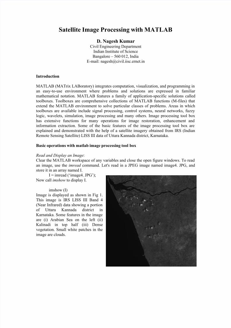
Image is displayed as shown in Fig 1.

This image is IRS LISS III Band 4

(Near Infrared) data showing a portion

of Uttara Kannada district in

Karnataka. Some features in the image

are (i) Arabian Sea on the left (ii)

Kalinadi in top half (iii) Dense

vegetation. Small white patches in theimage are clouds.



2

Figure 1. Image displayed using imshow

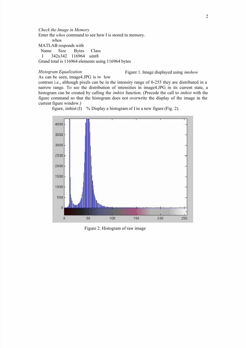
Figure 2. Histogram of raw image

Check the Image in Memory

Enter the whos command to see how I is stored in memory.

whos

MATLAB responds with

Name Size Bytes Class

I 342x342 116964 uint8

Grand total is 116964 elements using 116964 bytes

Histogram Equalization

As can be seen, image4.JPG is in low

contrast i.e., although pixels can be in the intensity range of 0-255 they are distributed in a

narrow range. To see the distribution of intensities in image4.JPG in its current state, a

histogram can be created by calling the imhist function. (Precede the call to imhist with the

figure command so that the histogram does not overwrite the display of the image in the

current figure window.)

figure, imhist (I) % Display a histogram of I in a new figure (Fig. 2).



3

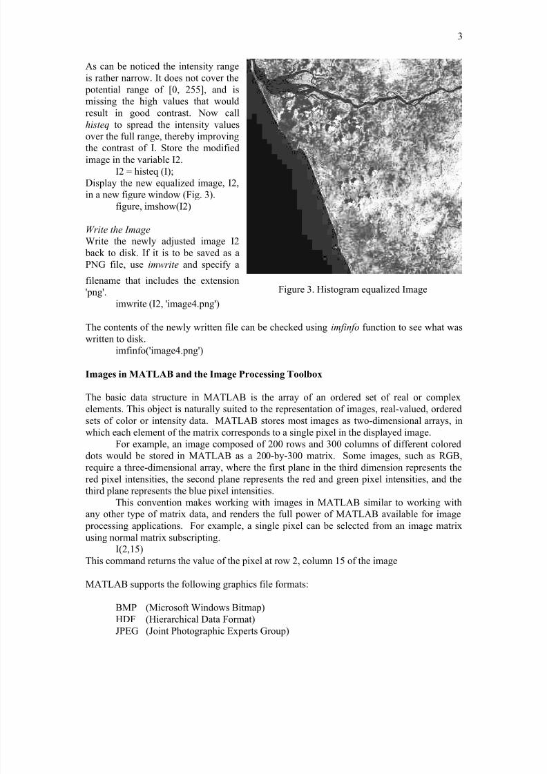
Figure 3. Histogram equalized Image

As can be noticed the intensity range

is rather narrow. It does not cover the

potential range of [0, 255], and is

missing the high values that would

result in good contrast. Now call

histeq to spread the intensity values

over the full range, thereby improvingthe contrast of I. Store the modified

image in the variable I2.

I2 = histeq (I);

Display the new equalized image, I2,

in a new figure window (Fig. 3).

figure, imshow(I2)

Write the Image

Write the newly adjusted image I2

back to disk. If it is to be saved as a

PNG file, use imwrite and specify a

filename that includes the extension

'png'.

imwrite (I2, 'image4.png')

The contents of the newly written file can be checked using imfinfo function to see what was

written to disk.

imfinfo('image4.png')

Images in MATLAB and the Image Processing Toolbox

The basic data structure in MATLAB is the array of an ordered set of real or complex

elements. This object is naturally suited to the representation of images, real-valued, orderedsets of color or intensity data. MATLAB stores most images as two-dimensional arrays, in

which each element of the matrix corresponds to a single pixel in the displayed image.

For example, an image composed of 200 rows and 300 columns of different colored

dots would be stored in MATLAB as a 200-by-300 matrix. Some images, such as RGB,

require a three-dimensional array, where the first plane in the third dimension represents the

red pixel intensities, the second plane represents the red and green pixel intensities, and the

third plane represents the blue pixel intensities.

This convention makes working with images in MATLAB similar to working with

any other type of matrix data, and renders the full power of MATLAB available for image

processing applications. For example, a single pixel can be selected from an image matrix

using normal matrix subscripting.I(2,15)

This command returns the value of the pixel at row 2, column 15 of the image

MATLAB supports the following graphics file formats:

BMP (Microsoft Windows Bitmap)

HDF (Hierarchical Data Format)

JPEG (Joint Photographic Experts Group)



4

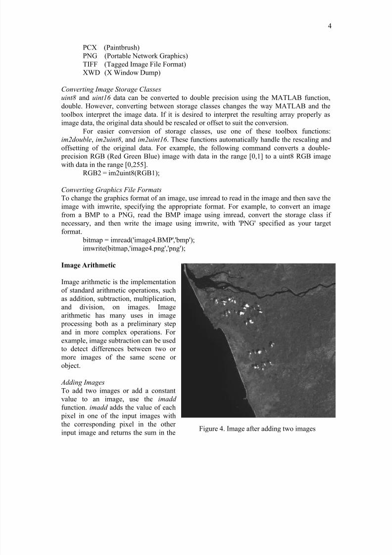
Figure 4. Image after adding two images

PCX (Paintbrush)

PNG (Portable Network Graphics)

TIFF (Tagged Image File Format)

XWD (X Window Dump)

Converting Image Storage Classes

uint8 and uint16 data can be converted to double precision using the MATLAB function,double. However, converting between storage classes changes the way MATLAB and the

toolbox interpret the image data. If it is desired to interpret the resulting array properly as

image data, the original data should be rescaled or offset to suit the conversion.

For easier conversion of storage classes, use one of these toolbox functions:

im2double, im2uint8, and im2uint16 . These functions automatically handle the rescaling and

offsetting of the original data. For example, the following command converts a double-

precision RGB (Red Green Blue) image with data in the range [0,1] to a uint8 RGB image

with data in the range [0,255].

RGB2 = im2uint8(RGB1);

Converting Graphics File Formats

To change the graphics format of an image, use imread to read in the image and then save the

image with imwrite, specifying the appropriate format. For example, to convert an image

from a BMP to a PNG, read the BMP image using imread, convert the storage class if

necessary, and then write the image using imwrite, with 'PNG' specified as your target

format.

bitmap = imread('image4.BMP','bmp');

imwrite(bitmap,'image4.png','png');

Image Arithmetic

Image arithmetic is the implementation

of standard arithmetic operations, suchas addition, subtraction, multiplication,

and division, on images. Image

arithmetic has many uses in image

processing both as a preliminary step

and in more complex operations. For

example, image subtraction can be used

to detect differences between two or

more images of the same scene or

object.

Adding Images

To add two images or add a constant

value to an image, use the imadd

function. imadd adds the value of each

pixel in one of the input images with

the corresponding pixel in the other

input image and returns the sum in the



5

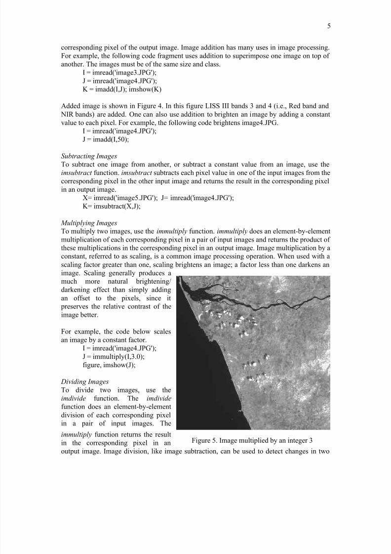
Figure 5. Image multiplied by an integer 3

corresponding pixel of the output image. Image addition has many uses in image processing.

For example, the following code fragment uses addition to superimpose one image on top of

another. The images must be of the same size and class.

I = imread('image3.JPG');

J = imread('image4.JPG');

K = imadd(I,J); imshow(K)

Added image is shown in Figure 4. In this figure LISS III bands 3 and 4 (i.e., Red band and

NIR bands) are added. One can also use addition to brighten an image by adding a constant

value to each pixel. For example, the following code brightens image4.JPG.


J = imadd(I,50);

Subtracting Images

To subtract one image from another, or subtract a constant value from an image, use the

imsubtract function. imsubtract subtracts each pixel value in one of the input images from the

corresponding pixel in the other input image and returns the result in the corresponding pixel

in an output image.

X= imread('image5.JPG'); J= imread('image4.JPG');

K= imsubtract(X,J);

Multiplying Images

To multiply two images, use the immultiply function. immultiply does an element-by-element

multiplication of each corresponding pixel in a pair of input images and returns the product of

these multiplications in the corresponding pixel in an output image. Image multiplication by a

constant, referred to as scaling, is a common image processing operation. When used with a

scaling factor greater than one, scaling brightens an image; a factor less than one darkens an

image. Scaling generally produces a

much more natural brightening/

darkening effect than simply addingan offset to the pixels, since it

preserves the relative contrast of the

image better.

For example, the code below scales

an image by a constant factor.


J = immultiply(I,3.0);

figure, imshow(J);

Dividing Images

To divide two images, use the

imdivide function. The imdivide

function does an element-by-element

division of each corresponding pixel

in a pair of input images. The

immultiply function returns the result

in the corresponding pixel in an

output image. Image division, like image subtraction, can be used to detect changes in two



6

Figure 6. Pixel coordinates

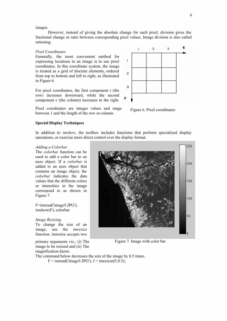
Figure 7. Image with color bar

images.

However, instead of giving the absolute change for each pixel, division gives the

fractional change or ratio between corresponding pixel values. Image division is also called

rationing.

Pixel Coordinates

Generally, the most convenient method for expressing locations in an image is to use pixel

coordinates. In this coordinate system, the image

is treated as a grid of discrete elements, ordered

from top to bottom and left to right, as illustrated

in Figure 6.

For pixel coordinates, the first component r (the

row) increases downward, while the second

component c (the column) increases to the right.

Pixel coordinates are integer values and range

between 1 and the length of the row or column.

Special Display Techniques

In addition to imshow, the toolbox includes functions that perform specialized display

operations, or exercise more direct control over the display format.

Adding a Colorbar

The colorbar function can be

used to add a color bar to an

axes object. If a colorbar is

added to an axes object thatcontains an image object, the

colorbar indicates the data

values that the different colors

or intensities in the image

correspond to as shown in

Figure 7.

F=imread('image5.JPG');

imshow(F), colorbar

Image Resizing

To change the size of animage, use the imresize

function. imresize accepts two

primary arguments viz., (i) The

image to be resized and (ii) The

magnification factor.

The command below decreases the size of the image by 0.5 times.

F = imread('image5.JPG'); J = imresize(F,0.5);



7

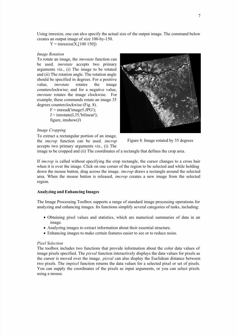
Figure 8. Image rotated by 35 degrees

Using imresize, one can also specify the actual size of the output image. The command below

creates an output image of size 100-by-150.

Y = imresize(X,[100 150])

Image Rotation

To rotate an image, the imrotate function can be used. imrotate accepts two primary

arguments viz., (i) The image to be rotated

and (ii) The rotation angle. The rotation angle

should be specified in degrees. For a positive

value, imrotate rotates the image

counterclockwise; and for a negative value,

imrotate rotates the image clockwise. For

example, these commands rotate an image 35

degrees counterclockwise (Fig. 8).

F = imread('image5.JPG');

J = imrotate(I,35,'bilinear');

figure, imshow(J)

Image Cropping

To extract a rectangular portion of an image,

the imcrop function can be used. imcrop

accepts two primary arguments viz., (i) The

image to be cropped and (ii) The coordinates of a rectangle that defines the crop area.

If imcrop is called without specifying the crop rectangle, the cursor changes to a cross hair

when it is over the image. Click on one corner of the region to be selected and while holding

down the mouse button, drag across the image. imcrop draws a rectangle around the selected

area. When the mouse button is released, imcrop creates a new image from the selectedregion.

Analyzing and Enhancing Images

The Image Processing Toolbox supports a range of standard image processing operations for

analyzing and enhancing images. Its functions simplify several categories of tasks, including:

• Obtaining pixel values and statistics, which are numerical summaries of data in an

image.

• Analyzing images to extract information about their essential structure.

• Enhancing images to make certain features easier to see or to reduce noise.

Pixel Selection

The toolbox includes two functions that provide information about the color data values of

image pixels specified. The pixval function interactively displays the data values for pixels as

the cursor is moved over the image. pixval can also display the Euclidean distance between

two pixels. The impixel function returns the data values for a selected pixel or set of pixels.

You can supply the coordinates of the pixels as input arguments, or you can select pixels

using a mouse.



8

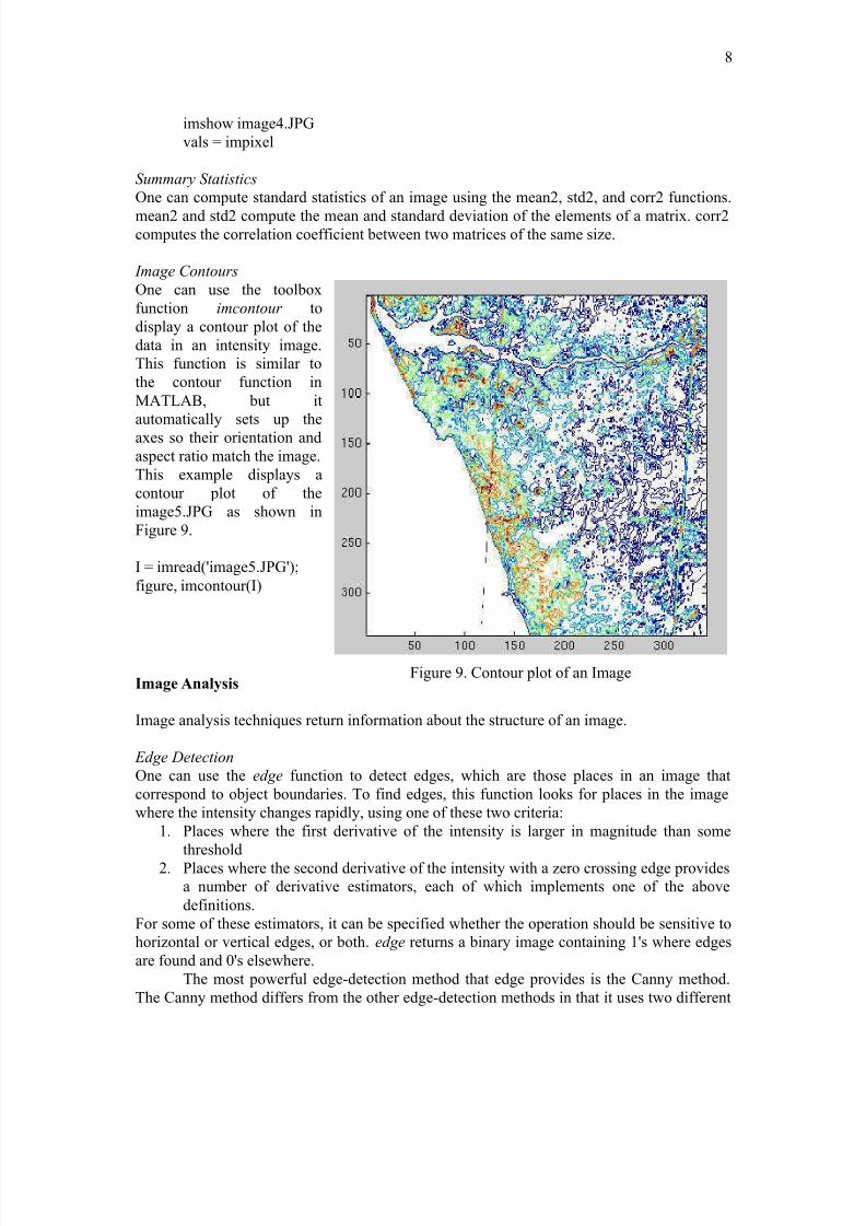
Figure 9. Contour plot of an Image

imshow image4.JPG

vals = impixel

Summary Statistics

One can compute standard statistics of an image using the mean2, std2, and corr2 functions.

mean2 and std2 compute the mean and standard deviation of the elements of a matrix. corr2computes the correlation coefficient between two matrices of the same size.

Image Contours

One can use the toolbox

function imcontour to

display a contour plot of the

data in an intensity image.

This function is similar to

the contour function in

MATLAB, but it

automatically sets up the

axes so their orientation and

aspect ratio match the image.

This example displays a

contour plot of the

image5.JPG as shown in

Figure 9.


figure, imcontour(I)

Image Analysis

Image analysis techniques return information about the structure of an image.

Edge Detection

One can use the edge function to detect edges, which are those places in an image that

correspond to object boundaries. To find edges, this function looks for places in the image

where the intensity changes rapidly, using one of these two criteria:

1. Places where the first derivative of the intensity is larger in magnitude than some

threshold2. Places where the second derivative of the intensity with a zero crossing edge provides

a number of derivative estimators, each of which implements one of the above

definitions.

For some of these estimators, it can be specified whether the operation should be sensitive to

horizontal or vertical edges, or both. edge returns a binary image containing 1's where edges

are found and 0's elsewhere.

The most powerful edge-detection method that edge provides is the Canny method.

The Canny method differs from the other edge-detection methods in that it uses two different



9

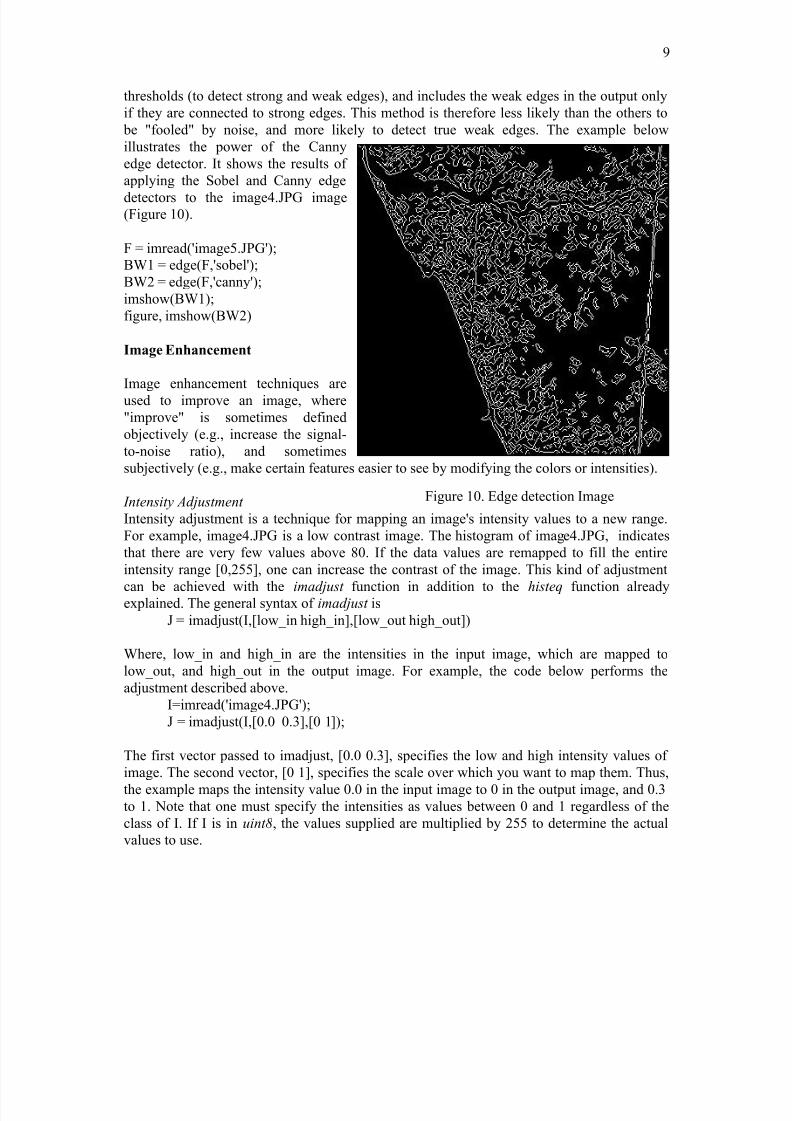
Figure 10. Edge detection Image

thresholds (to detect strong and weak edges), and includes the weak edges in the output only

if they are connected to strong edges. This method is therefore less likely than the others to

be "fooled" by noise, and more likely to detect true weak edges. The example below

illustrates the power of the Canny

edge detector. It shows the results of

applying the Sobel and Canny edge

detectors to the image4.JPG image(Figure 10).

F = imread('image5.JPG');

BW1 = edge(F,'sobel');

BW2 = edge(F,'canny');

imshow(BW1);

figure, imshow(BW2)

Image Enhancement

Image enhancement techniques are

used to improve an image, where

"improve" is sometimes defined

objectively (e.g., increase the signal-

to-noise ratio), and sometimes

subjectively (e.g., make certain features easier to see by modifying the colors or intensities).

Intensity Adjustment

Intensity adjustment is a technique for mapping an image's intensity values to a new range.

For example, image4.JPG is a low contrast image. The histogram of image4.JPG, indicates

that there are very few values above 80. If the data values are remapped to fill the entire

intensity range [0,255], one can increase the contrast of the image. This kind of adjustment

can be achieved with the imadjust function in addition to the histeq function alreadyexplained. The general syntax of imadjust is

J = imadjust(I,[low_in high_in],[low_out high_out])

Where, low_in and high_in are the intensities in the input image, which are mapped to

low_out, and high_out in the output image. For example, the code below performs the

adjustment described above.

I=imread('image4.JPG');

J = imadjust(I,[0.0 0.3],[0 1]);

The first vector passed to imadjust, [0.0 0.3], specifies the low and high intensity values of

image. The second vector, [0 1], specifies the scale over which you want to map them. Thus,

the example maps the intensity value 0.0 in the input image to 0 in the output image, and 0.3

to 1. Note that one must specify the intensities as values between 0 and 1 regardless of the

class of I. If I is in uint8, the values supplied are multiplied by 255 to determine the actual

values to use.



10

To use imadjust , one must typically perform two steps:

1. View the histogram of the image to determine the intensity value limits.

2. Specify these limits as a fraction between 0.0 and 1.0 so that you can pass them to

imadjust in the [low_in high_in] vector.

MATLAB image processing tool box has many more capabilities and only a small portion of

them is explained in this article.

Bibliography

MathWorks Inc., Image Processing Tool Box Users Guide, 2001.

image processing matlab

Documents