image processing for optical metrology - intech -...
TRANSCRIPT

25
Image Processing for Optical Metrology
Miguel Mora-González, Jesús Muñoz-Maciel, Francisco J. Casillas, Francisco G. Peña-Lecona, Roger Chiu-Zarate
and Héctor Pérez Ladrón de Guevara Universidad de Guadalajara, Centro Universitario de los Lagos
México
1. Introduction
Optical measurements offer the desirable characteristics of being noninvasive and nondestructive techniques that are able to analyze in real time objects and phenomena in a remote sense. Science areas that involve optical characterization include physics, biology, chemistry and varied fields of engineering. The use of digital cameras to record objects or a specific phenomenon permits the exploitation of the potential of that the associated images can be processed to determine one or several parameter or characteristics of what is being recorded. These images need to be processed and securely there will be a model associated with the optical metrology that will provide an insight or a comprehensive understanding of the image being analyzed. Matlab® is the suitable platform to implement image processing algorithms due to its ability to perform the whole processing techniques and procedures to analyze and image. At the same time it provides a flexible and a fast programming language for user constructing algorithms. In the present chapter we provide some fundamentals about image acquisition, filtering and processing, and some applications. Some applications are well-know techniques while others offer the state of the art in the field under study. All authors agree that Matlab® is a powerful tool for image processing and optical metrology. All algorithms and/or sentences used in this chapter are made in such manner so that they work in the Matlab® R2007b platform or superior. Matlab® is a trade mark of Mathworks Inc., from here on we will refer it as Matlab only. Also the Matlab functions and parameters used along the chapter are typed in italics and in apostrophes, respectively. Algorithms in present chapter are presented in two formats depending on the algorithm extension: 1) Image titles and/or figure captions for low algorithms extension; 2) Subsection ends for larger algorithms.
2. Image processing and acquisition
In the present section, image and processing acquisition principles in Matlab are established.
2.1 Image acquisition Image acquisition is the initial stage in every vision system for human or artificial image data interpretation. Image acquisition is the recording process of a real object, this implies
www.intechopen.com

MATLAB – A Ubiquitous Tool for the Practical Engineer
524
that the vision process totally depends on quality acquisition; this could be an analogical or digital. The analogical acquisition process is a representation of the object with several techniques like designing, painting, photography, and video. In a similar way, digital imaging acquisition is able to represent a real object, however object properties are presented in a discrete form. Every object characteristics are mapped from a real plane to a digital plane where a group of discrete values (i.e 1, 2, 3, …,) represent position, form, color and texture.
2.1.1 Acquisition and digital image representation Image acquisition process in Matlab can be done by the use of either imread or getsnapshot functions for stored images or video, respectively. Each function stores the object representation in a discrete lxmxn array, where l can be related to color data; m and n indexes represent the image spatial coordinates. An example of a real image is shown in Figure 1a, and in Figure 1b, the representation in a matrix array of the selected area from the image. Digital images are described as a bi-dimensional f(x,y) function, where x and y represent the spatial coordinates. The f value at the (x,y) position point is proportional to the intensity or gray scale of the image. In Matlab, a digital image satisfies following conditions: first, spatial and gray scale values must be discrete; and second, intensities are sampling at 8 bits (255 values).
Fig. 1. a) real color image, and b) matrix of the green color component of the selected area.
2.1.2 Image discretization Image discretization is the process of converting an analogical image to a digital image; this process depends on the sampling and quantization stages. Correspondence between analogical and digital images is given by the number of pixels used. If the number of pixels is enough to satisfy the Nyquist criteria (Oppenheim et al., 1997), the acquired image is a satisfactory representation of the real object observed. Quantization is the process of assigning a color or gray discrete level to each sample. Therefore, image discretization quality depends on frequency sampling as in quantization levels used. It must be noted that Matlab only reads digital images. Acquisition process can be done with scanners, CCD cameras, etc.
2.2 Thresholding and high contrast image Frequently, acquired images under real conditions present a background problem. When relevant foreground elements are mixed with low interest background ones. Another
www.intechopen.com

Image Processing for Optical Metrology
525
problem that hides the desired information is a low contrast image. Therefore, the use of algorithms that deals with can be implemented in order to enhance the images. Equalization, binarization and thresholding algorithm are alternatives that have proved to be successful. In the following subsection, a method for the conversion of color images into gray levels is presented. Next, by using histogram equalization, a high contrast image from the gray scale levels is obtained. Finally, binarization process by establishing a thresholding is described in order to get a two color image (black (0) and white (255)) from a gray level scale (Poon & Banerjee, 2001).
2.2.1 Histogram Histogram is the graphical representation of pixels gray values distribution. Images can be classified according to its histogram as high, medium or low contrast images. A low contrast image has a histogram with a low fraction of all possible gray values, around less than 40% of the whole scale. A high contrast image has more than 90% of the gray values. Color images can also be classified in accordance with its histogram by considering human ocular sensitivity to primary colors. This is given by the first component of the YIQ matrix:
0.299 0.587 0.114 ,Y R G B= + + (1)
Where Y and RGB are the lumma components used in color television systems NTSC (that represents a gray scale in the YIQ space) and the primary components, red, green and blue, respectively. The histogram transformation for a color image is given by the following pixel to pixel operation:
( ) ,gsl k kT r s= (2)
where rk and sk are the original pixel intensities in color and gray scale levels (gsl) respectively. In figure 2 is shown the image obtained by the use of equation (2) and its corresponding histogram, these operations can be done by using the Matlab functions rgb2gray and imhist.
Fig. 2. a) gsl photography, b) histogram.
2.2.2 Histogram equalization Histogram equalization is the transformation of the intensity values of an image that is typically applied to enhance the contrast of the image. As an example, the contrast of the
www.intechopen.com

MATLAB – A Ubiquitous Tool for the Practical Engineer
526
image of the figure 2a, can be handled by applying histogram equalization and it is shown in figure 3 with its respective histogram, this operation can be done by using the Matlab function histeq.
Fig. 3. a) Photography equalization, b) histogram.
In order to get the discrete values in a gsl, the following equation is used
0
( ) ( 1),k
jeq k
j
nT s L
n== −∑ (3)
where k = 0,1,2,…, (L-1), L represents the gray level numbers into an image (255 as an example), nj is the frequency of appearance of an specific j-th gray level and n is the total number of pixels of the image.
2.2.3 Thresholding by histogram Thresholding is a non-linear operation for image segmentation that consists in the conversion of a gsl image into a binary image according to a threshold value. This operation is used to separate some regions of the foreground of an image from its background. Thresholding operation can be done by using the Matlab function graythresh. Binarization may be considered as an especial case of thresholding as shown in figure 4. The Matlab function that binaries an image is im2bw.
Fig. 4. Image binarization by thresholding.
2.3 Spatial filtering In order to reduce noise or enhance some specific characteristics of an image some filters like high-pass, low-pass, band-pass or band-stop are used. These filters can be applied in the
www.intechopen.com

Image Processing for Optical Metrology
527
frequency domain (section 2.4) or in the spatial domain. Spatial domain filtering is described in this section. Filtering operations are directly applied to the image (pixel to pixel). The mathematical functions applied in the spatial domain are well known as convolution, and are described by (Mora-González et al., 2008)
1 12 2
1 12 2
( , ) * ( , ) ( , ) ( , ),
M N
M Nm n
f x y g x y f m n g x m y n+ +
+ +=− =−= − −∑ ∑ (4)
where f, g,(x,y), (m,n) and MxN are the original image, the convolution mask or matrix, the original image coordinates, the coordinates where the convolution is performed, and the size of convolution mask, respectively. Equation (4) is applied by doing a homogeneous scanning with the convolution mask versus the whole image to be convolved. These filters are also known as Finite Impulse Response (FIR) filters because they are applied to a finite section of the spatial domain (In this case the finite section is the image). Equation (4) can be implemented in Matlab by using nested for loops, also conv2, fspecial or imfilter functions can be used too. These kinds of filters are dependent of the convolution mask form as is explained in the following two subsections.
2.3.1 Low-pass filters Low-pass filters applied to images have the purpose of image smoothing, by blurring the edges into the image and lowering the contrast. The main characteristic of a low-pass convolution mask is that all of its elements have positive values. Some commonly used low-pass filters are: averaging, gaussian, quadratic, triangular and trigonometric. These mask are presented in a matrix form like
1,1 1,2 1,
2,1 2,2 2,
,,1 ,2 ,1 1
1( , ) ,
N
NM N
m nM M M Nm n
w w w
w w wg m n
ww w w= =
⎡ ⎤⎢ ⎥⎢ ⎥= ⎢ ⎥⎢ ⎥⎢ ⎥⎣ ⎦∑∑……
B B D B…
(5)
with
( ) ( )( ) ( )
( ) ( )
2 21 12 2
2 21 12 2
1 12 4 2 4 2
exp ,
1 , ,
cos cos ,
,
M N
M N
M NA A A
A B m n gaussian
A B m B n cuadraticw
B m B n trigonometric
A average
+ +
+ +
+ +
⎧ ⎫⎛ ⎞⎡ ⎤− − + −⎜ ⎟⎪ ⎪⎢ ⎥⎣ ⎦⎝ ⎠⎪ ⎪⎪ ⎪⎡ ⎤⎪ ⎪− − − −= ⎢ ⎥⎨ ⎬⎣ ⎦⎪ ⎪⎡ ⎤ ⎡ ⎤+ − + −⎪ ⎪⎣ ⎦ ⎣ ⎦⎪ ⎪⎪ ⎪⎩ ⎭
(6)
where A, B and w are the amplitude, the width function factor and the weight function of the spatial filter, respectively. In order to determine the effectiveness of the masks of the equations (5) and (6), Magnitude Spectra (MS) are obtained to analyze the low frequencies allowed to pass by the filter and high frequencies attenuation. This is expressed as
{ }( ) 20log ( , ) ,MS g m nω = ℑ (7)
www.intechopen.com

MATLAB – A Ubiquitous Tool for the Practical Engineer
528
where ω and ℑ are the MS frequency component and the Fourier transform operator, respectively. In figure 5, the MS of the convolution mask from equations (5) and (6) are shown. Spatial
gaussian filter behavior is more stable because allows low frequencies to pass and also
attenuate middle and high frequencies faster than other filters, as can be observed. The mask
for nine elements is shown in table 1. It must be mentioned that the processing time slow
down conforming the convolution mask increases. Spatial filtering also has a problem in the
image edges, because they cannot be convolved and there are (M-1)/2 and (N-1)/2 lost
information elements in x and y axes, respectively. By using the fspecial function, low-pass
masks can be generated by applying the ‘gaussian’ or ‘average’ Matlab parameters.
Another mask types designed for signal processing can be implemented on image processing by a two dimensional extension. In figure 6 it is shown three different low-pass filters applied in the test image.
Fig. 5. MS of equations (5) and (6) masks, with A=1, B=1 and w=1. Matlab code representation of equation (7) is: MS=20*log10(abs(fft(g))).
Gaussian Quadratic Trigonometric Average
.0449 .1221 .0449
.1221 .3319 .1221
.0449 .1221 .0449
⎛ ⎞⎜ ⎟⎜ ⎟⎜ ⎟⎝ ⎠
0 .1667 0
.1667 .3333 .1667
0 .1667 0
⎛ ⎞⎜ ⎟⎜ ⎟⎜ ⎟⎝ ⎠
.1011 .1161 .1011
.1161 .1312 .1161
.1011 .1161 .1011
⎛ ⎞⎜ ⎟⎜ ⎟⎜ ⎟⎝ ⎠
1 1 11
1 1 19
1 1 1
⎛ ⎞⎜ ⎟⎜ ⎟⎜ ⎟⎝ ⎠
Table 1. 3x3 convolution masks g for low-pass filters of equations (5) and (6), with A=1, B=1 and w=1.
Fig. 6. Low-pass 3x3 filters examples applied to figure 1a. Matlab parameters used: a) average, b) gaussian and c) disk.
www.intechopen.com

Image Processing for Optical Metrology
529
2.3.2 High-pass filters High frequency components are mostly located in image borders, like fast tone changes and marked details. The main purpose of a high-pass filter is to highlight the image details for skeletonizing, geometrical orientation, contrast enhancement, and revealing hidden characteristics, among many others. One of the most common high-pass spatial filters is the high-boost that consists in an interactive subtraction process between the original image and low-pass filters. The weighting function for a 3x3 matrix is obtained by
19
19
9 , 2, 2.
, 2, 2
C m nw
m n
⎧ − = =⎪= ⎨ − ≠ ≠⎪⎩ (8)
The differential filters are another kind of high-pass filters that get its weighting function
based on the partial derivates applied to the image. The most usual differential filters are the
gradient and laplacian, based on the following equations
22
( ( , )) , ,f f f f
f x y gradient magnitudex y x y
⎛ ⎞∂ ∂ ∂ ∂⎛ ⎞∇ = + ≈ +⎜ ⎟⎜ ⎟∂ ∂ ∂ ∂⎝ ⎠ ⎝ ⎠ (9)
and
2 2
22 2
( ( , )) , ,f f
f x y laplacianx y
∂ ∂∇ = +∂ ∂ (10)
if the magnitude of the partial derivatives work with a 3x3 mask, then
1,3 2,3 3,3 1,1 2,1 3,1
1( ) ( )
2
fw w w w w w
xκ κκ
∂ ⎡ ⎤= + ⋅ + − + ⋅ +⎣ ⎦∂ + (11)
and
1,1 1,2 1,3 3,1 3,2 3,3
1( ) ( ) .
2
fw w w w w w
yκ κκ
∂ ⎡ ⎤= + ⋅ + − + ⋅ +⎣ ⎦∂ + (12)
Other used filters based on gradients are the Sobel, Prewitt and Canny. The Sobel spatial
filter uses the central weight constant k=2 (Pratt, 2001). Meanwhile the Pewwit space filter
uses k=1. The Canny space filter uses two different thresholds for weak and strong edges
detection (Canny, 1986). Table 2 shows the nine elements masks of the most utilized high-
pass filters. Figure 7 shows six examples of the application of these functions as high-pass
filters to figure 1a. It is observed that the Canny filter is the most powerful edge detector
filter.
2.4 Mathematical discrete transforms Discrete transform analysis has played an important role in digital image processing.
Several transform types are applicable to digital image processing, but due to their optical
metrology potential applications, Fourier and Radon transforms are presented in this
chapter section.
www.intechopen.com

MATLAB – A Ubiquitous Tool for the Practical Engineer
530
2.4.1 Fourier transform Discrete Fourier Transform (DFT) represents the change from spatial to frequency domain. In convergent optical systems this transform represents the propagated optical perturbation from exit pupil to the focal point in a single lens arrangement. Equations (13) and (14) represent the DFT pair for the mathematical two dimensional (2D) model (Gonzalez, 2002)
{ } ( )1 1
1( , ) ( , ) ( , )exp 2 ,
M Nvyux
M Nx y
f x y F u v f x y iMN
π= =
⎡ ⎤ℑ = = − +⎢ ⎥⎣ ⎦∑∑ (13)
Sobel Prewitt Gradient Laplacian
fx∂∂ =
1 0 1
2 0 2
1 0 1
−−−
⎛ ⎞⎜ ⎟⎜ ⎟⎜ ⎟⎝ ⎠
fy∂∂ =
1 2 1
0 0 0
1 2 1− − −
⎛ ⎞⎜ ⎟⎜ ⎟⎜ ⎟⎝ ⎠
fx∂∂ =
1 0 1
1 0 1
1 0 1
−−−
⎛ ⎞⎜ ⎟⎜ ⎟⎜ ⎟⎝ ⎠
fy∂∂ =
1 1 1
0 0 0
1 1 1− − −
⎛ ⎞⎜ ⎟⎜ ⎟⎜ ⎟⎝ ⎠
fx∂∂ =
1 1 1
1 2 1
1 1 1
−− −
−
⎛ ⎞⎜ ⎟⎜ ⎟⎜ ⎟⎝ ⎠
fy∂∂ =
1 1 1
1 2 1
1 1 1
⎛ ⎞⎜ ⎟−⎜ ⎟⎜ ⎟− − −⎝ ⎠
0 1 0
1 4 1
0 1 0
−⎛ ⎞⎜ ⎟⎜ ⎟⎜ ⎟⎝ ⎠
Table 2. Some 3x3 convolution masks g for high-pass differential filters (Bow, 2002).
Fig. 7. High-pass 3x3 filters examples applied to figure 1a. Matlab parameters and functions used: a) ‘canny’, b) ‘sobel’, c) ‘prewitt’, d) laplacian with ‘log’, e) gradient and f) high-boost filter.
and
{ } ( )1
1 1
( , ) ( , ) ( , )exp 2 ,M N
vyuxM N
u v
F u v f x y F u v i π−= =
⎡ ⎤ℑ = = +⎢ ⎥⎣ ⎦∑∑ (14)
www.intechopen.com

Image Processing for Optical Metrology
531
where (u,v), MxN and ℑ-1 are the Fourier space coordinates, the image size, the inverse
Fourier transform operator, respectively. Matlab has fft2 and ifft2 special functions for
equations (13) and (14), respectively, where FFT is the acronyms of Fast Fourier Transform.
Other functions of Fourier transforms are fft, ifft for one dimension, and fftshift for the
shifting of the zero-frequency component to spectra center. An important characteristic
obtained from the Fourier transform is that it gives the frequencies content of the image.
Due to this property, frequency filter design is a very straight forward task. Low frequencies
are located into the matrix around the central coordinates, while frequencies gradually
increase as are spread out from its center in a radial form. This characteristic is ideal for
frequency filtering (low-pass, high-pass, band-pass, and band-stop). The frequency filtering
process consists in the multiplication between image Fourier transform with a binary
circular mask. Figure 8 shows the filtered Fourier spectra and the resulting filtered images
for a high-pass, low-pass, band-pass and band-stop.
Fig. 8. Fourier filtering applied to figure 1a. a) high-pass, b) low-pass, c) band-pass and d) band-stop. Where, circle and ring are masks of 30 and 60 pixels radii.
2.4.2 Radon transform Radon transform applied in pattern recognition or digital image processing may be
considered as the image’s gsl projection over a given angle with respect to x axis. The
mathematical model of the Radon transform is (Bracewell, 1995)
{ } ( )( , ) ( , ) cos sin ,f x y f x y R x y dxdtδ θ θ∞ ∞
−∞ −∞ℜ = − −∫ ∫ (15)
where ℜ, δ, R and θ are the Radon transform operator, the Dirac delta function, the distance
from the origin to the profile line and the angle of direction of the same line, respectively.
Each of these parameters can be observed in figure 9, Q is the origin of the profile line to be
obtained (thick blue bold line). Equation (15) is implemented in Matlab with the special
function radon.
www.intechopen.com

MATLAB – A Ubiquitous Tool for the Practical Engineer
532
Fig. 9. Radon transform parameters.+
3. Optical metrology fundamentals
Optical metrology is a field of physics that include theoretical and experimental methods to estimate physical parameters using the light wavelength as fundamental scale.
3.1 Optical interferometry Optical interferometry is based in the light interference phenomenon to determine different physical variables. A typical application is in nondestructive optical testing that requires high accuracy. The interferometer is the optical system used by this technique, which allows by interfering fringes the estimation of deformation components, shapes, strains or vibrations in objects with polished or rough surfaces. According to users’ requirements, different configurations of interferometers can be selected to measure displacements components.
3.1.1 Interference Figure 10 shows the schematic of a common optical arrangement used in interferometry well known as Michelson interferometer. The beam splitter (BS) splits the incident collimated laser light in two wavefronts that propagate in different directions and are reflected by the plane mirrors M1 and M2 respectively, and then they are combined with the same BS to form an interference pattern that can be observed directly on the screen.
Fig. 10. Michelson interferometer.
The superposition of the two wavefrons at a position (x,y) is expressed by the complex sum:
www.intechopen.com

Image Processing for Optical Metrology
533
1 1 2 2( , ) ( , )exp[ ( , )] ( , )exp[ ( , )],= +U x y a x y i x y a x y i x yφ φ (16)
where a1(x,y) and a2(x,y) are the amplitudes and its respective phases φ1(x,y) y φ2(x,y). The intensity at a point in the interference pattern is determined with the product of perturbation U multiplied by its complex conjugated U*, this is
*( , ) ( , ) ( , ),I x y U x y U x y= ⋅ (17)
then, the resulting intensity is given by
1 2 1 2( , ) ( , ) ( , ) 2 ( , ) ( , ) cos[ ( , )],= + +I x y I x y I x y I x y I x y x yφ (18)
where I1(x,y)=a12(x,y) and I2(x,y)=a12(x,y) are the intensities for each wavefront and φ(x,y) is the phase difference between them, since these propagate along to different paths before the interference.
Due to cosine of equation (18), I(x,y) reaches its maxima when φ(x,y) corresponds to even
multiples of π (constructive interference) and its minima for odd multiples of π (destructive interference) (Gasvik, 2002). In general, optical interferometry is applied to estimate this phase difference, which can arise due to geometrical variations or deformations in a testing object. In figure 11 are shown two synthetic interference patterns when is replaced a mirror: a) with tilt in y and defocus and b) with defocus and coma in the interferometer of figure 10. The phase difference involving the geometrical variations of the mirrors is given by φ(x,y)=4πΔz/λ, where λ is the wavelength of the illumination source and Δz is the shape phase difference introduced by the mirrors.
Fig. 11. Fringe patterns of mirrors with: a) tilt in y and defocus, YD; and b) defocus and coma, DC. These wavefronts were generated using nested for loops. For these cases N=128 pixels; C1=0.01 and C2= 0.00001 are the numerical parameter of each aberration.
Another way to generate fringe patterns is by replacing a mirror of the interferometer for a testing object with an optically rough surface that experiments a deformation. In this case, the interference fringe pattern is not observed directly on the screen as in the previous described case. The superposition of a wavefront reflected by a rough surface (object beam) with a regular wavefront (reference beam) as the reflected by a plane mirror in the
Michelson interferometer causes that I1, I2 and φ of equation (18) vary fast and randomly, normally obtaining a speckle pattern. In speckle pattern interferometry the fringe patterns are obtained by the correlation of two speckle patterns recorded using a CCD camera placed at the screen position of the interferometer for the object before and after a deformation Δφ(x,y). Assuming Ii(x,y), If(x,y) are the intensities of the speckle patterns for the initial no-
www.intechopen.com

MATLAB – A Ubiquitous Tool for the Practical Engineer
534
deformed state and the final deformed state respectively, the fringe patter can be calculated by (Lehmann, 2001)
( , ) ( , ) ,f iI x y I x y− (19)
and the phase difference involving the deformation of the object is given by Δφ(x,y)=4πz’/λ, where z’ is the displacement of the object in z direction (Waldner, 2000).
3.1.2 Phase shifting
In order to determine the phase φ(x,y) from fringe patterns, is applied a procedure well-known as phase shifting. For this procedure can be registered several images introducing a phase difference which experimentally is achieved with a piezoelectric (PZ) that modifies the optical path length of one of the beams. A widely used algorithm to calculate the phase employs four consecutive images shifted by π/2 (Huntley, 2001)
1 ( , ) ( , )( , ) tan ,
( , ) ( , )− ⎡ ⎤−= ⎢ ⎥−⎣ ⎦
d b
a c
I x y I x yx y
I x y I x yφ (20)
where Ia(x,y), Ib(x,y), Ic(x,y) and Id(x,y) are the intensities of the shifted images. Due to the inverse tangent, in this pattern arise an effect of wrapping in a 2π module; moreover can be affected by noise of high frequency in the case of speckle interferograms. If the interest of the user is to explore the reduction of speckle noise and phase unwrapping techniques can consults references (Sirohi, 1993) and (Ghiglia, 1998). In figure 12 are shown the wrapped phases calculated with equation (20) using the fringe patterns presented in the section.
3.2 Image diffraction The mathematical representation for a collimated wavefront passing through a convergent optical system until the focal point is given by the Fourier transform, as is observed in figure 13. By setting a diffraction grating in the entrance pupil of a convergent lens, a Fraunhofer diffraction pattern is obtained in the focal point (Goodman, 2005), given by
( ) ( )2 2
2exp
( , ) ( , ) exp ,f
o f
A j u vU u v r x y j xu yv dxdy
j f
πλ πλλ∞
−∞
⎡ ⎤⋅ +⎣ ⎦ ⎡ ⎤= ⋅ − +⎣ ⎦∫ ∫ (21)
Fig. 12. Calculated wrapped phases for: a) tilt in y and defocus, wpYD; and b) defocus and coma, wpDC.
www.intechopen.com

Image Processing for Optical Metrology
535
where Uo(u, v), r(x, y), A and λ are the complex amplitude distribution of the field in the back focal plane of the lens, the grating function, the amplitude of the monochromatic plane wave and the illumination wavelength, respectively. The result of equation (21) varies depending on the function of the grating. For our purposes, those functions are binary and sinusoidal.
Fig. 13. Diagram for performing the Fourier transform of a grating with a positive lens.
3.2.1 Binary grating A binary grating can be mathematically represented by a Fourier series expansion of a step function (fstep) bounded in the [0,T] interval, see figure 14a. The function is defined by:
2
2
, 0( , ) ,
0,
T
step T
a yf x y
y T
⎧ < <⎪= ⎨ ≤ ≤⎪⎩ (22)
and its Fourier series expansion is given by (Tolstov, 1962)
02,
[( 1) 1]( , ) exp[ ( )],
(2 )
n
binm n
ar x y i mx ny
mnωπ
∞=−∞
− −= +∑ (23)
where T and a are the grating period and the amplitude, respectively. Then the intensity profile at the focal plane is calculated from equations (17) and (21), with r(x,y) as vertical binary grating of equation (23), giving (Mora-González et al., 2009)
( ) ( )0
2
220
2
sin( , ) , ,
kbin K
k
kI u v h Ku K v
k
π ωπ δ∞
=−∞⎛ ⎞ ⎡ ⎤⎜ ⎟= ⋅ −⎢ ⎥⎣ ⎦⎜ ⎟⎝ ⎠∑ (24)
here 22
0Aafh πλ= is the zero diffraction order amplitude, 2
fK πλ= is the scale factor at the focal
plane and 20 T
πω = is the angular frequency. The binary grating intensity profile presents an
infinite number of diffraction orders (harmonics) modulated by a sinc function (see figure 14b).
3.2.2 Sinusoidal grating In order to observe the sinusoidal grating profile, it must be above x axis because negative
gsl cannot be observed. The equation proposed for the vertical sinusoidal grating is given by
(see figure 14c)
www.intechopen.com

MATLAB – A Ubiquitous Tool for the Practical Engineer
536
( )1 1sin 02 2
( , ) sin .r x y a yω⎡ ⎤= +⎣ ⎦ (25)
The intensity profile at the focal plane from equation (21) with r(x,y) as vertical sinusoidal grating of equation (25), giving (Mora-González et al., 2009)
( ) [ ] ( )0 02 2 2sin 1 0 1( , ) , , , ,K KI u v h Ku K v h Ku Kv h Ku K vω ωδ δ δ⎡ ⎤ ⎡ ⎤= + + + −⎢ ⎥ ⎢ ⎥⎣ ⎦ ⎣ ⎦ (26)
where 2
1Aa
fh πλ= is the ±1 sinusoidal diffraction orders amplitude. The sinusoidal grating
intensity profile only presents three diffraction orders (see figure 14d), those harmonics are characteristic of the Fourier transform of sinusoidal functions.
Fig. 14. Functions of a) binary and c) sinusoidal gratings. Fourier spectra of b) binary and d) sinusoidal gratings.
4. Aplications
As shown in previous sections, Digital Image Processing is a useful tool to obtain improved results in Optical Metrology. Applications details are presented in following subsections.
4.1 Fringe analysis Fringe analysis refers to the process of finding the phase associated to physical variables that are being estimated. A typical case consists in the interpretation of the fringe patterns that can be achieved with phase shifting techniques, when the object under study remains static while three or more frames are acquired when the experiment conditions are free of environmental perturbations. Another case is when the environmental conditions are not met, and then the analysis of a single interferogram is more convenient. In both cases a wrapped phase is obtained before the related continuous phase is assessed. Phase unwrapping is a numerical technique for retrieving a continuous phase from the calculated phase by using the arctangent (atan2) of the sine and cosine functions of the phase. In its simplest form, phase unwrapping consists in the addition or subtraction of a 2π multiple when a discontinuity bigger than π is found between adjacent pixels (Robinson, 1993). This approach however is very sensitive to noise, and is said to be path dependent. It means that any error may propagate along the path followed to phase unwrapping. In this study we will review the least square method (Ghiglia, 1998). Basically, it consists in the integration of the phase gradient by solving a linear equation system employing a numerical technique. Lets assume φx(x,y) and φy(x,y) as the phase differences in the horizontal and vertical directions, respectively. These phases are calculated from the wrapped phase φw(x,y) as follows:
www.intechopen.com

Image Processing for Optical Metrology
537
1sin ( , ) ( 1, )
( , ) tan ( , ) ( 1, ),cos ( , ) ( 1, )
− ⎧ ⎫⎡ ⎤− −⎪ ⎪⎣ ⎦= −⎨ ⎬⎡ ⎤− −⎪ ⎪⎣ ⎦⎩ ⎭w w
xw w
x y x yx y p x y p x y
x y x y
φ φφ φ φ (27)
and
1sin ( , ) ( , 1)
( , ) tan ( , ) ( , 1),cos ( , ) ( , 1)
− ⎧ ⎫⎡ ⎤− −⎪ ⎪⎣ ⎦= −⎨ ⎬⎡ ⎤− −⎪ ⎪⎣ ⎦⎩ ⎭w w
yw w
x y x yx y p x y p x y
x y x y
φ φφ φ φ (28)
In the above equations p(x,y) is a pupil function equal to one inside of an interferogram field
and zero otherwise. A discretized Laplacian equation is then obtained from the phase
differences:
( , ) ( 1, ) ( , ) ( , 1) ( , )
4 ( , ) ( 1, ) ( 1, ) ( , 1) ( , 1)
= + − + + −= − + + + − + + + −
y yx xL x y x y x y x y x y
x y x y x y x y x y
φ φ φ φφ φ φ φ φ . (29)
This equation represents a linear equations system that can be solved with iterative
algorithms. In particular, is employed an overrelaxation method (SOR) due to it may be
easily programmed. The following equation is then iterated until the solution converges:
1( , ) ( , )
( , ) ( 1, ) ( 1, ) ( , 1) ( , 1) ( , ),
+ = +⎡ ⎤− + − − − + − − +⎣ ⎦+
k k
k
x y x y
d x y x y x y x y x y L x y r
d
φ φφ φ φ φ φ (30)
where, d=p(x+1,y)+p(x-1,y)+p(x,y+1)+p(x,y-1), and r is a parameter of the SOR method that must be set between the [1,2] range. Figure 15 shows the wrapped phase φw obtained from the sine and cosine of the phase and the unwrapped phase φ. A simple iterative algorithm that unwraps the phase from the discretized Laplacian is given as: Algoritm 1. % Unwraps phase. while (q<max)%q is the number of iterations (500 for this case) q=q+1; for i=1:n for j=1:m if p(i,j)==1 t=p(i+1,j)+p(i-1,j)+p(i,j+1)+p(i,j-1); g(i,j)=g(i,j)-((t*g(i,j)-g(i+1,j)-g(i-1,j)-g(i,j+1)-g(i,j-1)+L(i,j))*1.95/t);%iterated equation else g(i,j)=0; end,end,end,end A single interferogram with open fringes may also be analyzed for phase recovering (Creath & Wyant, 1992). Experimentally an open fringe interferogram can be achieved if a tilt term is added to the phase, usually by tilting the reference beam in an interferometer. Equation (18) can be modified in order to include a tilt term in the x direction, this is as follows:
www.intechopen.com

MATLAB – A Ubiquitous Tool for the Practical Engineer
538
Fig. 15. a) wrapped and b) unwrapped phase.
[ ]( , ) ( , ) ( , )cos ( , ) 2= + +I x y a x y b x y x y txφ π (31)
where a(x,y)=I1(x,y)+I2(x,y) is known as the background intensity and b(x,y)=2[I1(x,y)I2(x,y)]½ is the modulation or visibility term. The Fourier transform of the expression below can be written as:
( , ) ( , ) ( , ) * ( , ).I u v a u v C u t v C u t v= + + + −# # (32)
Then the Fourier spectra of an open fringe interferogram contains three terms, ã(u,v) is a narrow peak at the center of the Fourier spectra and C(u+t,v) and C*(u-t,v) are shifted complex conjugate intensities symmetrically located respect to the origin of the Fourier
Fig. 16. Process of phase recovery from a single interferogram with closed fringes, as shown in algorithm 2. a) Interferogram, b) Fourier spectrum, c) filtered Fourier spectrum, d) wrapped phase with tilt, e) wrapped phase without tilt, and f) unwrapped continuous phase.
www.intechopen.com

Image Processing for Optical Metrology
539
domain (Takeda, 1982). The Fourier procedure to recover the phase consist in isolating either C(u,v) or C*(u,v). Then the inverse transform is taken in order to retrieve the wrapped phase from the imaginary and real parts of the filtered spectra. The last step, as done with phase shifting procedures, is to apply a phase unwrapping procedure to recover the continuous phase. The complete process of phase recovery from an open fringe interferogram is observed in figure 16. Algoritm 2. % Phase recovery from a single interferogram for i=1:256 for j=1:256 if sqrt((i-128)^2+(j-128)^2)<126 %creates a function pupil pupil(i,j)=1; else pupil(i,j)=0; end x=(i-128)/128; y=(j-128)/128; phase(i,j)=2*pi*(4*(x^2+y^2)+16*x); g(i,j)=2*pi*16*x; back(i,j)=128*exp(-1*(x^2+y^2)); mod(i,j)=127*exp(-1*(x^2+y^2)); I(i,j)=(back(i,j)+mod(i,j)*cos(phase(i,j)))*pupil(i,j); % Interferogram with closed fringes H(i,j)=exp(-180*((x-0.25)^2+y^2));%Band-Pass filter G(i,j)=1-exp(-1000*(x^2+y^2));%High pass filter end,end IF=fftshift(fft2(I));%Fourier transform of the interferogram IFH=IF.*H.*G; %Filtered Fourier transform Ih=ifft2(fftshift(IFH)); %Inverse Filtered Fourier transform fw=atan2(imag(Ih),real(Ih)).*pupil;%Wrapped phase with tilt fw1=atan2(sin(fw-g),cos(fw-g)).*pupil; %Wrapped phase without tilt phase1=(phase-g).*pupil; %Unwrapped phase
4.2 Wavefront deformation analysis Optical metrology applied for the determination of different physical variables has greatly
contributed with the constant advance of technology at a point that it is becoming a
powerful measurement alternative for the solution of problems in engineering and sciences.
4.2.1 Deformation analysis using speckle interferometry In this section, is presented a deformation analysis for the estimation of out-of-plane
displacement components in a simulated model of a cantilever made of aluminum with a
load applied at its free end. The example corresponds to a typical problem in structural
mechanics where the Young´s modulus can be determined from the displacement of the
loaded bar made of an isotropic material. The suggested arrangement for the testing in
electronic speckle pattern interferometry (ESPI) is shown in figure 17. The laser light beam is
divided by the beam splitter BS1. One beam is reflected by a mirror attached to a
piezoelectric PZ (PC controlled), and then is expanded to uniformly illuminate at a small
www.intechopen.com

MATLAB – A Ubiquitous Tool for the Practical Engineer
540
angle respect to the normal of the object surface, and the other beam is coupled into an
optical fiber to obtain the reference illumination. The light reflected by the object and the
reference beam introduced with BS2 interfere on the CCD.
Fig. 17. Electronic speckle pattern interferometer.
The object was simulated by considering the following dimensions: 15 cm length and 3 cm height with a thickness of 0.5 cm. Using the two intensities Ii(x,y), If(x,y) of the speckle patterns generated by ESPI arrangement seen in the CCD image plane before and after applying a force of 0.1 N, the correlation fringes using equation (19) is shown in figure 18a and in figure 18b is shown the wrapped phase calculated by equation (20). In figure 18c is shown the filtered and unwrapped phase using a conventional spatial average filter of 3 x 3 pixels and an iterative least-squares algorithm.
Fig. 18. Deformation analysis of a cantilever with ESPI. a) interference fringe pattern; b) wrapped phase and c) unwrapped phase.
4.3 Wavefront detection Optical testing using diffraction gratings as wavefront modulators is another alternative to detect wavefront aberrations.
4.3.1 Grating diffraction Diffraction gratings are optical devices commonly used on physics. There are several gratings types, but as shown in 3.2 section, sinusoidal gratings only diffracts three harmonic
www.intechopen.com
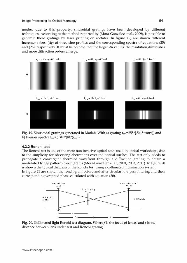
Image Processing for Optical Metrology
541
modes, due to this property, sinusoidal gratings have been developed by different techniques. According to the method reported by (Mora-González et al., 2009), is possible to generate these gratings by laser printing on acetates. In figure 19, are shown different
increment sizes (Δy) of three sine profiles and the corresponding spectra of equations (25)
and (26), respectively. It must be pointed that for larger Δy values, the resolution diminishes and more diffraction orders emerge.
Fig. 19. Sinusoidal gratings generated in Matlab. With a) grating rsin=255*[.5+.5*sin(y)] and b) Fourier spectra Isin=fftshift(fft2(rsin)).
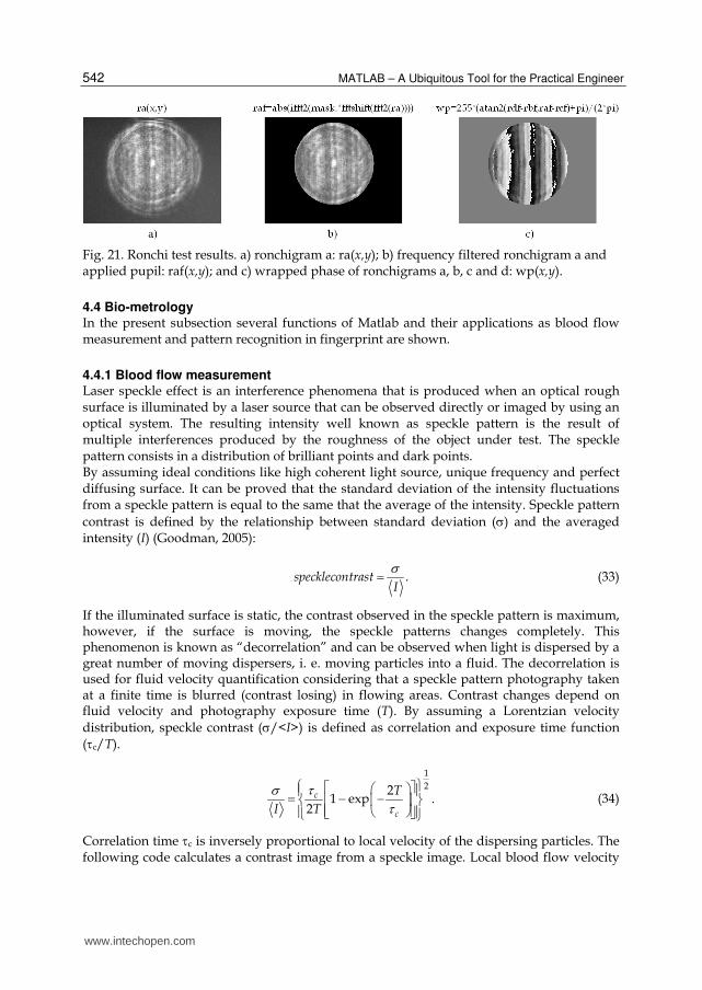
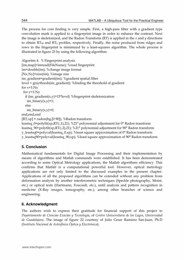
4.3.2 Ronchi test The Ronchi test is one of the most non invasive optical tests used in optical workshops, due to the simplicity for observing aberrations over the optical surface. The test only needs to propagate a convergent aberrated wavefront through a diffraction grating to obtain a modulated fringe pattern (ronchigram) (Mora-González et al., 2001, 2003, 2011). In figure 20 is shown the typical diagram of the Ronchi test using a collimated illumination system. In figure 21 are shown the ronchigram before and after circular low-pass filtering and their corresponding wrapped phase calculated with equation (20).
Fig. 20. Collimated light Ronchi test diagram. Where f is the focus of lenses and r is the distance between lens under test and Ronchi grating.
www.intechopen.com
MATLAB – A Ubiquitous Tool for the Practical Engineer
542
Fig. 21. Ronchi test results. a) ronchigram a: ra(x,y); b) frequency filtered ronchigram a and applied pupil: raf(x,y); and c) wrapped phase of ronchigrams a, b, c and d: wp(x,y).
4.4 Bio-metrology In the present subsection several functions of Matlab and their applications as blood flow measurement and pattern recognition in fingerprint are shown.
4.4.1 Blood flow measurement Laser speckle effect is an interference phenomena that is produced when an optical rough surface is illuminated by a laser source that can be observed directly or imaged by using an optical system. The resulting intensity well known as speckle pattern is the result of multiple interferences produced by the roughness of the object under test. The speckle pattern consists in a distribution of brilliant points and dark points. By assuming ideal conditions like high coherent light source, unique frequency and perfect diffusing surface. It can be proved that the standard deviation of the intensity fluctuations from a speckle pattern is equal to the same that the average of the intensity. Speckle pattern
contrast is defined by the relationship between standard deviation (σ) and the averaged intensity (I) (Goodman, 2005):
.specklecontrastIσ= (33)
If the illuminated surface is static, the contrast observed in the speckle pattern is maximum, however, if the surface is moving, the speckle patterns changes completely. This phenomenon is known as “decorrelation” and can be observed when light is dispersed by a great number of moving dispersers, i. e. moving particles into a fluid. The decorrelation is used for fluid velocity quantification considering that a speckle pattern photography taken at a finite time is blurred (contrast losing) in flowing areas. Contrast changes depend on fluid velocity and photography exposure time (T). By assuming a Lorentzian velocity
distribution, speckle contrast (σ/<I>) is defined as correlation and exposure time function (τc/T).
1
221 exp .
2c
c
TI T
τστ
⎫⎧ ⎡ ⎤⎛ ⎞⎪ ⎪= − −⎢ ⎥⎜ ⎟⎨ ⎬⎢ ⎥⎝ ⎠⎪ ⎪⎣ ⎦⎩ ⎭ (34)
Correlation time τc is inversely proportional to local velocity of the dispersing particles. The following code calculates a contrast image from a speckle image. Local blood flow velocity
www.intechopen.com

Image Processing for Optical Metrology
543
can be found from image contrast information and equation (34). Figure 22 shown speckle images before and after processing. Algoritm 3. % Calculation of speckle contrast. Im2 = imread('speckle_img.bmp'); % load the bmp image file into the memory. Im2 = im2double(Im2); windowSize = 5; %define the window size for the filter. avgFilter = fspecial('average',windowSize); % generate an averaging filter. stdSpeckle = stdfilt(I,ones(windowSize)); %caculates the local standar deviation of image. avgSpeckle = imfilter(I,avgFilter,'symmetric'); %calculates the average of each pixel ctrSpeckle = stdSpeckle./avgSpeckle; %caculates the speckle contrast image
Fig. 22. Blood flow measurement results. a) speckle image of a rat cortex. b) speckle image of contrast after processing with the code of algoritm 3.
4.4.2 Fingerprint measurement Several applications in pattern recognition are also utilized in optical metrology, finger print parameters measurements is an example. The present subsection shows a new form for fingerprint core determination based in the Radon transform of a fingerprint image, applied in x and y axes directions. The core is located by the interception of the extremes (local minimum and maximum) of the Radon transforms (Mora-González et al., 2010).
Fig. 23. Images for fingerprint core point detection. a) original fingerprint im(x,y), b) gradient of original fingerprint im_gradient(x,y), and c) binarized gradient im_binary(x,y) and its 0° - 90° Radon transforms.
www.intechopen.com
MATLAB – A Ubiquitous Tool for the Practical Engineer
544
The process for core finding is very simple. First, a high-pass filter with a gradient type
convolution mask is applied to a fingerprint image in order to enhance the contrast. Next
the image is skeletonized, and the Radon Transform (RT) is applied in the x and y directions
to obtain RT90 and RT0 profiles, respectively. Finally, the noise produced from ridges and
rows in the fingerprint is minimized by a least-squares algorithm. The whole process is
illustrated in figure 23 by using the following algorithm:
Algoritm 4. % Fingerprint analysis.
[im,map]=imread(FileName); %read fingerprint
im=double(im); %change image format
[Nx,Ny]=size(im); %image size
im_gradient=gradient(im); %gradient spatial filter
level = graythresh(im_gradient); %finding the threshold of gradient
for x=1:Nx
for y=1:Ny
if (im_gradient(x,y)>15*level) %fingerprint skeletonization
im_binary(x,y)=1;
else
im_binary(x,y)=0;
end,end,end
[RT,xp] = radon(bg,[0 90]); %Radon transform
leastsq_0=polyfit(xp,RT(:,1),21); %21° polynomial adjustment for 0° Radon transform
leastsq_90=polyfit(xp,RT(:,2),21); %21° polynomial adjustment for 90° Radon transform
y_leastsq0=polyval(leastsq_0,xp); %least square approximation of 0° Radon transform
y_leastsq90=polyval(leastsq_90,xp); %least square approximation of 90° Radon transform
5. Conclusion
Mathematical fundamentals for Digital Image Processing and their implementation by
means of algorithms and Matlab commands were established. It has been demonstrated
according to some Optical Metrology applications, the Matlab algorithms efficiency. This
confirms that Matlab is a computational powerful tool. However, optical metrology
applications are not only limited to the discussed examples in the present chapter.
Applications of all the proposed algorithms can be extended without any problem from
deformation analysis by another interferometric techniques (Speckle photography, Moiré,
etc.) or optical tests (Hartmann, Foucault, etc.), until analysis and pattern recognition in
medicine (X-Ray images, tomography, etc.), among other branches of science and
engineering.
6. Acknowledgment
The authors wish to express their gratitude for financial support of this project to
Departamento de Ciencias Exactas y Tecnología, of Centro Universitario de los Lagos, Universidad de Guadalajara. The image of figure 22 courtesy of Julio Cesar Ramirez San-Juan, Ph.D
(Instituto Nacional de Astrofísica Óptica y Electrónica).
www.intechopen.com

Image Processing for Optical Metrology
545
7. References
Bow, S.T. (2002). Pattern Recognition and Image Preprocesing (2nd Ed.), Marcel Dekker, Inc., ISBN 0-8247-0659-5, New York, USA.
Bracewell, R.N. (1995). Two-Dimensional Imaging, Prentice Hall, ISBN 0-13-062621-X, New Jersey, USA.
Canny, J. (1986). A Computational Approach to Edge Detection, IEEE Trans. on Pattern Analysis and Machine Intelligence, Vol.PAMI-8, No.6, (November 1986), pp. 679-698, ISSN 0162-8828.
Creath, K.; Schmit, J. and Wyant, J.C. (2007), Optical Metrology of Diffuse Surfaces, In: Optical Shop Testing, 3th ed., Malacara, D., pp. 756-807, John Wiley & Sons, Inc., ISBN 978-0-471-48404-2, Hoboken, New Jersey, USA.
Gasvik, K.J. (2002). Optical Metrology, John Wiley & Sons, Ltd., ISBN 0-470-84300-4, Chichester, West Sussex, England.
Ghiglia, D.C., Pritt, M.D. (1998), Two-Dimensional Phase Unwrapping: Theory Algorithms and Software, Wiley-Interscience, ISBN 0-471-24935-1, New York, USA.
Gonzalez, R.C. & Woods, R.E. (2002). Digital Image Procesing (2nd Ed.), Prentice Hall, ISBN 0-201-18075-8, New Jersey, USA.
Goodman, J.W. (2005). Introduction to Fourier Optics (3rd Ed.), Roberts and Company Publishers, ISBN 0-9747077-2-4, Englewood, USA.
Huntley, J. M. (2001), Automated analysis of speckle interferograms, In: Digital Speckle Patter Interferometry and Related Techniques, Rastogi, P. K., pp. 59-140, John Wiley & Sons, Ltd., ISBN 0-471-49052-0, Chichester, West Sussex, England.
Lehmann, M. (2001). Speckle Statistics in the Context of Digital Speckle Interferometry, In: Digital Speckle Patter Interferometry and Related Techniques, Rastogi, P. K.¸ pp. 1-58, John Wiley & Sons, Ltd., ISBN 0-471-49052-0, Chichester, West Sussex, England.
Mora González, M. & Alcalá Ochoa, N. (2001). The Ronchi test with an LCD grating, Opt. Comm., Vol.191, No.4-6, (May 2001), pp. 203-207, ISSN 0030-4018.
Mora-González, M. & Alcalá Ochoa, N. (2003). Sinusoidal liquid crystal display grating in the Ronchi test, Opt. Eng., Vol.42, No.6, (June 2003), pp. 1725-1729, ISSN 0091-3286.
Mora-González, M.; Casillas-Rodríguez, F.J.; Muñoz-Maciel, J.; Martínez-Romo, J.C.; Luna-Rosas, F.J.; de Luna-Ortega, C.A.; Gómez-Rosas, G. & Peña-Lecona, F.G. (2008). Reducción de ruido digital en señales ECG utilizando filtraje por convolución, Investigación y Ciencia, Vol.16, No.040, (September 2008), pp. 26-32, ISSN 1665-4412.
Mora-González, M.; Pérez Ladrón de Guevara, H.; Muñoz-Maciel, J.; Chiu-Zarate, R.; Casillas, F.J.; Gómez-Rosas, G.; Peña-Lecona, F.G. & Vázquez-Flores, Z.M. (2009). Discretization of quasi-sinusoidal diffraction gratings printed on acetates, Proceedings of SPIE 7th Symposium Optics in Industry, Vol.7499, 74990C, ISBN 978-0-8194-8067-5, Guadalajara, México, September 2009.
Mora-González, M.; Martínez-Romo, J.C.; Muñoz-Maciel, J.; Sánchez-Díaz, G.; Salinas-Luna, J.; Piza-Dávila, H.I.; Luna-Rosas, F.J. & de Luna-Ortega, C.A. (2010). Radon Transform Algorithm for Fingerprint Core Point Detection. Lecture Notes in Computer Science, Vol.6256, No.1, (September 2010), pp. 134-143, ISSN 0302-9743.
Mora-González, M.; Casillas, F.J.; Muñoz-Maciel, J.; Chiu-Zarate, R. & Peña-Lecona, F.G. (2011). The Ronchi test using a liquid crystal display as a phase grating, Proceedings of SPIE Optical Measurement Systems for Industrial Inspection VII, Vol.8082 part two, 80823G, ISBN 978-0-8194-8678-3, Münich, Germany, May 2011.
www.intechopen.com

MATLAB – A Ubiquitous Tool for the Practical Engineer
546
Oppenheim, A.V.; Willsky, A.S. & Nawab, S.H. (1997). Signasl and Systems, 2nd ed., Prentice Hall, Inc., ISBN 0-13-814757-4, New Jersey, USA.
Pratt, W.K. (2001). Digital Image Processing (3th Ed.), John Wiley & Sons, Inc., ISBN 0-471-22132-5, New York, USA.
Robinson, D.W. (1993). Phase unwrapping methods, In: Interferogram Analysis, Robinson, D.W. and Reid, G.T., pp. 195-229, IOP Publishing, ISBN 0-750-30197-X, Bristol, England.
Sirohi R. S. (1993), Speckle Metrology, Marcel Dekker, Inc., ISBN 0-8247-8932-6, New York, USA.
Takeda, M.; Ina, H. & Kobayashi, S. (1982). Fourier-transform method of fringe-pattern analysis for computer-based topography and interferometry, J. Opt. Soc. Am., Vol.72, No.1, (January 1982), pp. 156-160, ISSN 0030-3941.
Tolstov, G.P. (1962). Fourier Series, Dover Publications, Inc., ISBN 0-486-63317-9, New York, USA.
Waldner, S. P. (2000). Quantitative Strain Analysis with Image Shearing Speckle Pattern Interferometry (Shearography), Doctoral Thesis, Swiss Federal Institute of Technology, Zurich, Swiss.
www.intechopen.com

MATLAB - A Ubiquitous Tool for the Practical EngineerEdited by Prof. Clara Ionescu
ISBN 978-953-307-907-3Hard cover, 564 pagesPublisher InTechPublished online 13, October, 2011Published in print edition October, 2011
InTech EuropeUniversity Campus STeP Ri Slavka Krautzeka 83/A 51000 Rijeka, Croatia Phone: +385 (51) 770 447 Fax: +385 (51) 686 166www.intechopen.com
InTech ChinaUnit 405, Office Block, Hotel Equatorial Shanghai No.65, Yan An Road (West), Shanghai, 200040, China
Phone: +86-21-62489820 Fax: +86-21-62489821
A well-known statement says that the PID controller is the “bread and butter†of the control engineer. Thisis indeed true, from a scientific standpoint. However, nowadays, in the era of computer science, when thepaper and pencil have been replaced by the keyboard and the display of computers, one may equally say thatMATLAB is the “bread†in the above statement. MATLAB has became a de facto tool for the modernsystem engineer. This book is written for both engineering students, as well as for practicing engineers. Thewide range of applications in which MATLAB is the working framework, shows that it is a powerful,comprehensive and easy-to-use environment for performing technical computations. The book includesvarious excellent applications in which MATLAB is employed: from pure algebraic computations to dataacquisition in real-life experiments, from control strategies to image processing algorithms, from graphical userinterface design for educational purposes to Simulink embedded systems.
How to referenceIn order to correctly reference this scholarly work, feel free to copy and paste the following:
Miguel Mora-Gonza ́lez, Jesu ́s Mun ̃oz-Maciel, Francisco J. Casillas, Francisco G. Pen ̃a-Lecona, Roger Chiu-Zarate and He ́ctor Pe ́rez Ladro ́n de Guevara (2011). Image Processing for Optical Metrology, MATLAB - AUbiquitous Tool for the Practical Engineer, Prof. Clara Ionescu (Ed.), ISBN: 978-953-307-907-3, InTech,Available from: http://www.intechopen.com/books/matlab-a-ubiquitous-tool-for-the-practical-engineer/image-processing-for-optical-metrology