image decomposition and restoration using hlvese/papers/41624.pdf · image decomposition and...
TRANSCRIPT
IMAGE DECOMPOSITION AND RESTORATION USINGTOTAL VARIATION MINIMIZATION AND THE H−1 NORM∗
STANLEY OSHER† , ANDRES SOLE‡ , AND LUMINITA VESE†
MULTISCALE MODEL. SIMUL. c© 2003 Society for Industrial and Applied MathematicsVol. 1, No. 3, pp. 349–370
Dedicated to the memory of Andres Sole,
who died in a tragic accident soon after doing this work
Abstract. In this paper, we propose a new model for image restoration and image decompositioninto cartoon and texture, based on the total variation minimization of Rudin, Osher, and Fatemi[Phys. D, 60 (1992), pp. 259–268], and on oscillatory functions, which follows results of Meyer[Oscillating Patterns in Image Processing and Nonlinear Evolution Equations, Univ. Lecture Ser. 22,AMS, Providence, RI, 2002]. This paper also continues the ideas introduced by the authors in aprevious work on image decomposition models into cartoon and texture [L. Vese and S. Osher, J.Sci. Comput., to appear]. Indeed, by an alternative formulation, an initial image f is decomposedhere into a cartoon part u and a texture or noise part v. The u component is modeled by a functionof bounded variation, while the v component is modeled by an oscillatory function, bounded in thenorm dual to | · |H1
0. After some transformation, the resulting PDE is of fourth order, envolving the
Laplacian of the curvature of level lines. Finally, image decomposition, denoising, and deblurringnumerical results are shown.
Key words. total variation, image decomposition, cartoon, texture, restoration, partial differ-ential equation, functional minimization
AMS subject classifications. 35, 49
DOI. 10.1137/S1540345902416247
1. Introduction and motivations. An important task in image processing isthe restoration or reconstruction of a true image u from an observation f . Givenan image function f defined on Ω, with Ω ⊂ R
2 an open and bounded domain, theproblem is to extract u from f . The observation f is usually a noisy and/or blurredversion of the true image. In order to solve this inverse problem in the denoising case,one of the most well-known techniques is by energy minimization and regularization.To this end, for f ∈ L2(Ω), Rudin, Osher, and Fatemi [19] have proposed the followingminimization problem:
infuF (u) =
∫Ω
|∇u| + λ
∫Ω
|f − u|2dxdy.(1.1)
Here, λ > 0 is a weight parameter,∫Ω|f − u|2dxdy is a fidelity term, and
∫Ω|∇u|
is a regularizing term to remove the noise. The term∫Ω|∇u| is the total variation
of u. If u ∈ L1(Ω) and∫Ω|∇u| < ∞, then u ∈ BV (Ω), the space of functions of
bounded variation (the gradient is taken in the sense of measures). This space allowsfor discontinuities along curves; therefore edges and contours are kept in the image u,
∗Received by the editors October 16, 2002; accepted for publication (in revised form) May 5,2003; published electronically July 17, 2003.
http://www.siam.org/journals/mms/1-3/41624.html†Department of Mathematics, University of California Los Angeles, 405 Hilgard Avenue, Los An-
geles, CA 90095-1555 ([email protected], [email protected]). The research of the first authorwas supported in part by grants NSF DMS-0074735, ONR N00014-97-1-0027, and NIH P20MH65166.The research of the third author was supported in part by grants NSF ITR-0113439 and NIHP20MH65166.
‡The author is deceased. Former address: Departament de Tecnologia, Universitat Pompeu Fabra,Pg. de Circumval-lacio 8., Barcelona 08003, Spain. The research of this author was supported inpart by PNPGC project, reference number BFM2000-0962-C02-01.
349

350 STANLEY OSHER, ANDRES SOLE, AND LUMINITA VESE
which is the minimizer of this convex optimization problem. Existence and uniquenessresults of this minimization problem can be found in [1], [7], [20], [2].
Formally minimizing the functional (1.1) yields the associated Euler–Lagrangeequation:
u = f +1
2λdiv
( ∇u|∇u|
)in Ω,
∂u
∂n= 0 on ∂Ω.
This model performs very well for denoising of images, while preserving edges.However, smaller details, such as texture, are destroyed if the parameter λ is toosmall. To overcome this, Meyer [15] proposed a new minimization problem, changingin (1.1) the L2(Ω)-norm of (f − u) by a weaker norm, more appropriate to representtextured or oscillatory patterns. This is defined as follows [15].
Definition 1.1. Let G denote the Banach space consisting of all generalizedfunctions f(x, y) which can be written as
f(x, y) = ∂xg1(x, y) + ∂yg2(x, y), g1, g2 ∈ L∞(Ω),(1.2)
induced by the norm ‖f‖∗ defined as the lower bound of all L∞(Ω)-norms of thefunctions |g|, where g = (g1, g2), |g(x, y)| =
√g1(x, y)2 + g2(x, y)2, and where the
infimum is computed over all decompositions (1.2) of f .As Meyer mentions, the space G is the dual of the space W 1,1(Ω) (the set of
functions f such that ∇f ∈ L1(Ω)2). He also introduces two other spaces, denotedby F and E. The space F is defined as G, but now g1, g2 belong to the John andNirenberg space BMO(Ω), instead of L∞(Ω). Finally, the third space E consideredby Meyer is defined as G, but g1, g2 belong to the Besov space B−1,∞
∞ (Ω). E coincideswith B−1,∞
∞ (Ω).Meyer shows that if the component v := f − u represents texture or noise, then
it has to be modeled by one of these three larger spaces G,F,E. If f − u ∈ G, thenhe proposes the following new image restoration model:
infu
E(u) =
∫Ω
|∇u| + λ‖f − u‖∗.(1.3)
Note that this convex model cannot be solved directly, due to the form of the ∗-norm of (f − u). We cannot express directly the associated Euler–Lagrange equationwith respect to u.
In a recent work [21], the first and last authors have proposed a first practicalmethod to overcome this difficulty. They have proposed the following convex mini-mization problem, as an approximation of (1.3):
infu,g1,g2
Gp(u, g1, g2) =
∫Ω
|∇u| + λ
∫Ω
|f − (u+ ∂xg1 + ∂yg2)|2dxdy
+ µ
[∫Ω
(√g21 + g2
2
)p
dxdy
] 1p
,(1.4)
where λ, µ > 0 are tuning parameters, and p → ∞. As λ → ∞ and p → ∞, thefirst term ensures that u ∈ BV (Ω), and the second and third terms ensure thatdivg ≈ (f − u) ∈ G. The minimization is made with respect to u, g1, and g2. Threecoupled equations are then obtained from the computation of the associated Euler–Lagrange equations. In [21], image decomposition results into cartoon and texture,

IMAGE RESTORATION AND DECOMPOSITION 351
and applications to texture discrimination have been proposed. For more details, werefer the reader to [21]. Note that if in (1.4) we take p = 2, with v = divg, g ∈ L2(Ω),
then the quantity ‖v‖ = infg1,g2∈L2(Ω)
√∫Ω(g2
1 + g22)dxdy is exactly the seminorm of
H−1(Ω), the dual to H10 (Ω) (see, for instance, [10]). The minimization (1.4) yields the
decomposition f = u+ v+w, where u ∈ BV (Ω), v = divg with small ‖g‖Lp(Ω) norm,
and the residual w = − 12λdiv( ∇u
|∇u| ). In the limit, if λ → ∞, then ‖w‖L2(Ω) → 0.
In [21], very satisfactory results of image decomposition into cartoon plus texturehave been obtained even if λ is not too large.
In this paper, we propose an alternative practical approach, and we solve a sim-plified version of (1.3) and (1.4). We decompose f into u + v, with u ∈ BV (Ω), andv = P a generalized function (a distribution) with small norm, dual to the seminormof H1
0 (Ω). The precise formulation is given in the next section. Moreover, this newalgorithm is a decomposition of the form f = u + v, while the original method [21](which started this line of research) led to an f = u+ v+w model, with w a residualmade as small as possible by increasing λ. In fact, ‖w‖∗ ≤ 1
2λ (see [21]). The newalgorithm is simplified; the minimization is performed only with respect to one un-known, u, and an interesting and new fourth order equation is obtained, equivalentto the proposed minimization model.
Recent related work is as follows: in Bertalmio et al. [4], an application of themodel from [21] to image inpainting has been proposed. In Vese and Osher [22], themodel from [21] is further analyzed and developed. Also, the authors Aujol et al. [3]have recently proposed an interesting model for image decomposition, following [15]and [21].
Related PDEs of fourth order, arising in image analysis, can be found, for instance,in [7], [12], and [11].
For more related details on the topic of oscillations in nonlinear analysis, we referthe reader to [17]. Other works for restoration of textured images by total variationminimization, in a wavelet framework, are by Malgouyres [13], [14]. Also, texturemodeling by statistical methods was proposed by Zhu, Wu, and Mumford in [23], [24]and by Casadei, Mitter, and Perona in [5], among many others. In particular, werefer to Mumford and Gidas [16] for a stochastic model, in a related approach, fornatural images. For more related references, we refer the reader to [21] and referencestherein.
For related results, alternative methods, and image decomposition methods usingwavelets and harmonic analysis, we refer the reader to [15] and references therein.
The proposed new model is derived as follows.
2. Description of the proposed model. Assume that f −u = divg, with g ∈L2(Ω)2. We can then formally assume the existence of a unique Hodge decompositionof g as
g = ∇P + Q,
where P ∈ H1(Ω) is a single-valued function and Q is a divergence-free vector field.From here, we obtain that f−u = divg = P . Now, we express P = −1(f−u), andwe propose the following new convex minimization problem, a simplified and modifiedversion of (1.3):
infuE(u) =
∫Ω
|∇u| + λ
∫Ω
|∇(−1)(f − u)|2dxdy.(2.1)
352 STANLEY OSHER, ANDRES SOLE, AND LUMINITA VESE
This new minimization problem is obtained from (1.3) by neglecting Q from theexpression for g and by considering the (L2-norm)2 instead of the L∞-norm for |g|.
The precise formulations and assumptions are as follows. Consider the data
f ∈ BV (Ω) +
v ∈ L2(Ω),
∫Ω
v(x, y)dxdy = 0
.
Then, by the embedding of BV (Ω) into L2(Ω), we deduce that in fact f ∈ L2(Ω).We first recall the following theorem (see, for instance, [8]).Theorem 2.1. Let V0 = P ∈ H1(Ω) :
∫ΩP (x, y)dxdy = 0. If v ∈ L2(Ω), with∫
Ωv(x, y)dxdy = 0, then the problem
−P = v,∂P
∂n|∂Ω = 0,(2.2)
admits a unique solution P in V0.Now, for each v ∈ L2(Ω), with
∫Ωv(x, y)dxdy = 0, there is a unique P with the
properties from Theorem 2.1. We will express this as P = −1v, and this gives asense to the last term in (2.1).
This new minimization problem can therefore be written using the norm inH−1(Ω), as defined by ‖v‖2
H−1(Ω) =∫Ω|∇(−1)v|2dxdy. Indeed, we can write
infuE(u) =
∫Ω
|∇u| + λ‖f − u‖2H−1(Ω).(2.3)
Formally minimizing (2.1), we obtain the Euler–Lagrange equation:
2λ−1(f − u) = div( ∇u|∇u|
),
∂u
∂n|∂Ω = 0,
∂div(
∇u|∇u|
)∂n
|∂Ω = 0.(2.4)
Instead of directly solving (2.4), we apply the Laplacian to (2.4) to obtain
2λ(u− f) = −[div
( ∇u|∇u|
)],
∂u
∂n|∂Ω = 0,
∂div(
∇u|∇u|
)∂n
|∂Ω = 0,(2.5)
which we shall solve by driving to steady state
ut = − 1
2λ[div
( ∇u|∇u|
)]− (u− f),
u(0, x, y) = f(x, y),∂u
∂n|∂Ω = 0,
∂div(
∇u|∇u|
)∂n
|∂Ω = 0.
Remark. The assumption that v := f − u satisfies∫Ω(f − u)dxdy = 0 is auto-
matically satisfied by (2.5). This can be simply obtained by integrating the PDE in(2.5) in space and using integration by parts and the boundary condition on the cur-vature operator, in the sense of distributions. Therefore, by our model, the residualv satisfies the property of noise or texture of being of zero mean.
Remark. Let us justify now our procedure of minimizing (2.1) in a simple generalframework to show that we still decrease the initial energy. Assume that we solve
infu
∫Ω
F (u)dxdy.

IMAGE RESTORATION AND DECOMPOSITION 353
Embedding the minimization in a dynamic scheme based on gradient descent, weobtain
ut = −Fu.
We then replace this last equation by
ut = Fu.
We show that the initial energy is still decreasing under the new flow. Indeed, wehave
d
dt
(∫Ω
F (u)dxdy
)=
∫Ω
Fuutdxdy =
∫Ω
FuFudxdy
=
∫Ω
div(Fu∇Fu)dxdy −∫
Ω
|∇Fu|2dxdy
=
∫∂Ω
Fu∂
∂n(Fu)dS −
∫Ω
|∇Fu|2dxdy.
This is a descent direction ( ddt (
∫ΩF (u)dxdy) < 0) if
(a) Fu = 0 or ∂∂ n (Fu) = 0 on ∂Ω,
(b) ∇Fu is not identically zero if Fu is not.The condition (a) ∂
∂ n (Fu) = 0 on ∂Ω is true in our framework. (b) is also true.We believe that it is remarkable that a TV minimization model leads to an equiva-
lent fourth order Euler–Lagrange PDE. Moreover, edges are kept in the u component,as we shall see in the numerical examples. Note that, by the Rudin–Osher–Fatemi(ROF) model, the curvature k = div( ∇u
|∇u| ), defined in the generalized sense, satisfies
k ∈ L2(Ω), while by the new model, k ∈ H1(Ω). So in the new model, the regular-ization is stronger than by the ROF model; therefore smaller details with the newmodel will be better separated from larger features. However, both models satisfy∫Ωk(x, y)dxdy = 0.We also have the following interesting property of the residual v := f − u, where
u is a minimizer of (2.1), giving information about vanishing moments. We state thissimple result in the following theorem.
Theorem 2.2. Assume f ∈ L2(Ω). For any subdomain Ω′ of Ω, if u is theformal solution of (2.4), then ∫
Ω′(f − u)wdxdy = 0
for each function w ∈ H1(Ω′) with w = 0 in Ω′, as long as K = 0 and ∂K∂n = 0 on
∂Ω′, where K denotes the curvature operator of level lines of u.Proof. The proof of this theorem can be obtained by multiplying (2.5) by w and
then integrating over Ω′ in space and applying integration by parts.We can also show existence of minimizers for (2.1) as follows.Theorem 2.3. For f ∈ BV (Ω) + v ∈ L2(Ω),
∫Ωv(x, y)dxdy = 0, the mini-
mization problem
infu
F (u) =
∫Ω
|∇u| + λ
∫Ω
|∇−1(f − u)|2dxdy,∫
Ω
(f − u)dxdy = 0
(2.6)
has a solution u ∈ BV (Ω).

354 STANLEY OSHER, ANDRES SOLE, AND LUMINITA VESE
Proof. Let un be a minimizing sequence of (2.6). Then there is a constant M > 0such that
∫Ω|∇un| ≤ M for all n ≥ 0. By the Poincare inequality, we obtain that
there is a positive constant C, depending only on Ω, such that∥∥∥un −∫Ωun
|Ω|∥∥∥L2(Ω)
≤ C
∫Ω
|∇u|.
Since∫Ωun =
∫Ωf , for all n ≥ 0, we deduce that un is uniformly bounded in
L2(Ω), and therefore in L1(Ω). Then we deduce that un is uniformly bounded inBV (Ω): there is a constant C ′ such that
‖un‖BV (Ω) = ‖un‖L1(Ω) +
∫Ω
|∇u| ≤ C ′.
Therefore, there is a subsequence of un, still denoted un, and u ∈ BV (Ω), such thatun → u strongly in L1(Ω) and weakly in BV − w∗, as n→ ∞. Moreover,∫
Ω
|∇u| ≤ lim infn→∞
∫Ω
|∇un|.
On the other hand, to each un of the minimizing and convergent subsequence (un)we can associate a unique Pn ∈ H1(Ω), such that f−un = −Pn, from Theorem 2.1.We have that ‖∇Pn‖2
L2(Ω) ≤ M , for all n ≥ 0, and also that∫ΩPndxdy = 0. Again,
by the Poincare inequality, we obtain that∥∥∥Pn −∫ΩPn
|Ω|∥∥∥L2(Ω)
= ‖Pn‖L2(Ω) ≤ C‖∇Pn‖2L2(Ω) ≤ C ′′
for all n ≥ 0. Therefore, there is a subsequence of Pn, still denoted Pn, and P ∈H1(Ω), such that Pn → P in L2(Ω), with
∫ΩPdxdy = 0. In fact, by uniqueness of
the limit, we need to have also f − u = −P . Therefore, we also have that
‖∇P‖2L2(Ω) = ‖∇−1(f − u)‖2
L2(Ω) ≤ lim infn→∞ ‖∇Pn‖2
L2(Ω) = ‖∇−1(f − un)‖2L2(Ω).
We finally deduce that
F (u) ≤ lim infn→∞ F (un);
therefore u is a minimizer of (2.6). Clearly,∫Ω(f − u)dxdy = 0.
We will present numerical results of image denoising, obtained using the model(2.5), in section 4. Comparison with the standard models of Rudin, Osher, andFatemi [19] and Vese and Osher [21] are also presented. We have also considered therestoration problem in the presence of both blur and noise. The original ROF modelfor restoring blurry, noisy imaging appeared in [18]. In this case, if K : L2(Ω) →L2(Ω) is a linear and continuous operator modeling the blur, and such that K∗, itsadjoint operator, commutes with the Laplacian , then the model for deblurring anddenoising is obtained in a similar manner: the convex energy to be minimized is
infuE(u) =
∫Ω
|∇u| + λ
∫Ω
|∇(−1)(f −Ku)|2dxdy.(2.7)
Following the same operations, we arrive at the transformed Euler–Lagrange equation
2λ(K∗Ku−K∗f) = −[div
( ∇u|∇u|
)].(2.8)

IMAGE RESTORATION AND DECOMPOSITION 355
We again solve this by our new descent procedure, which becomes
ut = − 1
2λ[div
( ∇u|∇u|
)]− (K∗Ku−K∗f), u(0, ·, ·) = f(·, ·).
Note that if K is a convolution operator, then it commutes with the Laplace operator.Following [7] and [20], under appropriate assumptions on K, it is possible to modifythe proof of Theorem 2.3 for the deblurring case (2.7).
Remark. We end this section by a simple but intuitive discussion and comparisonof the norms in H−1(Ω) used here and the G norm used by Meyer [15].
Consider v : [0, 1] → R such that∫ 1
0v(x)dx = 0. Then let g(x) =
∫ x
0v(ξ)dξ. Let
M , m be such that
M = g(x1) ≥ g(x) ≥ g(x2) = m for all x ∈ [0, 1].
Then
(A) g(x) =
∫ x
0
v(ξ)dξ −(M +m
2
)
has the smallest L∞[0, 1]-norm among all primitives of v, and
‖v‖∗ =M −m
2=
1
2
∫ x1
x2
v(ξ)dξ.
For example, if v = sin 2πnx, then ‖v‖∗ = ‖sin2πnx‖∗ = 14πn .
Next, let P be such that v = P ′′(x), with P ′(0) = P ′(1) = 0. Then P ′′ = g′, and
(B) g = P ′ =
∫ x
0
v(s)ds.
We have ‖v‖2H−1[0,1] = ‖g‖2
L2[0,1] =∫ 1
0(∫ x
0v(s)ds)2.
Note that the only difference between (A) and (B) is the constant M+m2 . Thus,
‖sin2πnx‖2H−1[0,1] =
∫ 1
0
(1 − cos 2πnx
2πn
)2
dx =1
4π2n2
3
2.
In two dimensions, on the unit square, we can write
v =
∞∑n,m=1
an,m cos 2πnx cos 2πmy.
Then
−1v = −∞∑
n,m=1
an,mcos 2πnx cos 2πmy
n2 +m2
and
‖∇−1v‖2L2(Ω) = π2
∞∑n,m=1
a2m,n
n2 +m2.
356 STANLEY OSHER, ANDRES SOLE, AND LUMINITA VESE
3. Some additional theoretical results. We present in this section some the-oretical results of the new model, similar to those mentioned by Meyer in [15], on theinitial ROF model. We recall the notation v := f − u, with u a minimizer.
(I) ‖−1f‖∗ ≤ 12λ if and only if u = 0, v = f .
(II) ‖−1f‖∗ > 12λ if and only if ‖−1v‖∗ = 1
2λ and
−∫
Ω
(−1v(x, y))u(x, y)dxdy =1
2λ‖u‖BV (Ω),
where ‖u‖BV (Ω) =∫Ω|∇u| (recall that v := f − u).
Proofs.(I) The minimizer is u = 0, v = f if and only if, for any h ∈ BV (Ω),
‖h‖BV + λ‖∇−1(f − h)‖22 ≥ λ‖∇−1f‖2
2.
Expanding this inequality, we obtain
‖h‖BV (Ω) + λ‖∇−1h‖22 ≥ −2λ
∫h(−1f)dxdy.
Replacing h first by +εh and then by −εh, and letting ε→ 0, we obtain
‖−1f‖∗ ≤ 1
2λ.
The inverse implication is also true: starting with this last inequality, then reversingthe steps, we arrive at the desired inequality using (a) the fact that −1f ∈ L2(Ω)and (b) Lemma 3 from [21].
(II) We have
‖u+ εh‖BV + λ‖∇(−1(v − εh))‖22 ≥ ‖u‖BV + λ‖∇−1v‖2
2;
then
‖u‖BV + |ε|‖h‖BV + λ‖∇(−1(v − εh))‖22 ≥ ‖u‖BV + λ‖∇−1v‖2
2.
Again, expand in the last inequality to get
|ε|‖h‖BV + λε2‖∇−1h‖22 ≥ −2ελ
∫h−1vdxdy.
Changing ε→ −ε and taking ε→ 0, we obtain, as before,
‖−1v‖∗ ≤ 1
2λ.
In the next step, we take h = u in the first equation above. If −1 < ε < 1, wehave
ε‖u‖BV + λε2‖∇−1u‖22 ≥ −2λε
∫u−1vdxdy.
If ε < 0, we have
‖u‖BV ≤ 2λ
∫u(−−1v)dxdy.

IMAGE RESTORATION AND DECOMPOSITION 357
If ε > 0, then
‖u‖BV ≥ 2λ
∫u(−−1v)dxdy,
and therefore∫u(−−1v)dxdy = 1
2λ‖u‖BV . This implies that ‖−1v‖∗ = 12λ .
Now, to verify the converse, we have
‖u+ εh‖BV + λ‖∇(−1(v − εh))‖22
≥ −2λ
∫(−1v)(u+ εh) + λ‖−1v‖2
2 + 2λε
∫(−1v)h+ λε2‖−1h‖2
2
= −2λ
∫(−1v)udxdy + λ‖−1v‖2
2 + λε2‖−1h‖22
= ‖u‖BV + λ‖−1v‖22 + λε2‖−1h‖2
2
≥ ‖u‖BV + λ‖−1v‖22.
In the case of restoration and deblurring, if
u = argminu
‖u‖BV + λ‖∇−1(Ku− f)‖22,
then the analogous results are as follows:(I) If ‖K∗−1f‖∗ ≤ 1
2λ , then u = 0 and v = f .
(II) If ‖K∗−1f‖∗ ≥ 12λ , then ‖K∗−1v‖∗ = 1
2λ and (u,K∗−1v) = − 12λ‖u‖BV .
The proofs for these results are similar.Remark. Following Chambolle [6], we have an interesting characterization of the
quantity v = f − u for u the minimizer of our variational problem (2.1):
v = P(1)K/2λ(−−1f) = argmin
w∈K/2λ
∫Ω
(∇(w + 2λ−1f))2dxdy.
Here
K = divg| g ∈ L2(Ω)2, ‖g‖∞ ≤ 1;
P(1)K/2λ is the H1 orthogonal projection onto K/2λ of −−1f . This result is obviously
closely related with the results (I) and (II) above, just as Chambolle’s original result [6]is related to Lemma 4 and Theorem 3, p. 32, of Meyer [15].
Again following Chambolle, we define
J(u) =
∫|∇u| = sup
∫Ω
udivξdxdy| ξ ∈ C1c (Ω), ‖ξ‖∞ ≤ 1
.
Then
J∗(u) = supu∈L2(Ω)
∫Ω
(uv − J(u))dxdy =
0 if v ∈ K,+∞ otherwise.
Minimizing the functional defined in (2.1) gives us
−2λ−1(f − u) ∈ ∂J(u),
358 STANLEY OSHER, ANDRES SOLE, AND LUMINITA VESE
where ∂J(u) is the subdifferential of the functional J(u) (see Ekeland and Temam [9]for the terminology). Since J is convex, by duality we obtain
u ∈ ∂J∗(−2λ−1(f − u))
or
0 ∈ 2λ(f − u) − 2λf + 2λ∂J∗(−2λ−1(f − u)).
Thus w = −2λ−1(f − u) is the minimizer of
‖∇(w + 2λ−1f)‖2
2+ 2λJ∗(w).
This is our desired result.
4. Numerical results for image restoration. We present in this section ournumerical results obtained with the proposed new model and comparisons with theTV model from [19]. In the experiments comparing our method with the classicalTV model, the parameter λ has been chosen such that the L2-norms of the v partscoincide. We also show comparisons with the original decomposition model introducedin [21].
In Figure 1, we show results obtained using both models on a textured imagewith a scale feature for different decreasing values of the parameter λ. The first rowshows the minimizer u, while the third row shows v := f − u, respectively. The sameexperiment has been performed using the classical TV model; the second row showsthe minimizer uTV , while the fourth row shows vTV := f − uTV . The parameter λfor the case of the TV model has been selected in each case in order to accomplish‖vTV ‖2 = ‖v‖2. We note that the new model separates better the textured detailsfrom the larger regions: the small textured details are in the v component, while thelarger regions are kept in the u component. Using the standard TV model, smalltextured details are still kept in the uTV component, while contours of larger regionscan be seen in the vTV component; therefore, the separation between texture andnontexture is not that well made using the standard TV model. These remarks canbe seen on the third column in Figure 1.
The same experiment has been performed on an image composed of four differentBrodatz textures (see Figure 2). The corresponding u, v, uTV , and vTV are displayedin Figure 3 (recall that in the TV result λ has been chosen such that ‖vTV ‖2 = ‖v‖2).The same remarks can be made by looking at these results: the new model separatesbetter the nontexture details, represented in u, from the texture details, representedin v (compare the right upper squares of the u components in Figure 3, top andbottom). We also show in Figure 4 the absolute value of v and vTV (after histogramequalization for visualization purposes).
Figure 5 corresponds to a real image where there is a high presence of texturescombined with nontextured parts. We have made the same kind of experiment as forthe Brodatz textures, which are shown in Figures 6 and 7, respectively. The u and vcomponents are displayed in Figure 6, while the absolute value of the v componentsis displayed in Figure 7. Again, we can make the same observation: the new modelseparates better the textured details shown in v from nontextured images kept in u.Indeed, if we look to the v components from Figure 6, we still see the hands in theresult produced by the standard TV model. These are not seen in the v componentproduced by the new model. On the other hand, details like the eyes are much better

IMAGE RESTORATION AND DECOMPOSITION 359
Fig. 1. Top: original grid image. First row: from left to right, computed u for λ =1, 0.1, 0.001, 0.0001 with the new model. Second row: computed u for the TV model. Third row:computed v for the new model. Fourth row: computed v for the TV model. In each case the TVresult has been computed such that the L2-norm of v is the same as in the new model.
kept in the u component of the new model. These remarks can also be noticed inFigure 7. In other words, the new model performs much better in keeping the maincontours in the u component, instead of the v component. The new model performsbetter for separating the main larger features from the textured features. We alsoshow in Figure 6 a comparison with the model from [21] (obtained very fast, using

360 STANLEY OSHER, ANDRES SOLE, AND LUMINITA VESE
Fig. 2. Original image composed of four different Brodatz textures.
only 100 time iterations). From these comparisons, we note that, on this image, thepresent new model has fewer edges in the v component, thus giving again a very goodresult. More comparisons with the original model [21] are presented in Figure 8, wherethe two image decomposition models give slightly different but comparable results.
Figures 9, 10, and 11 show the performance of the new model compared with theclassical TV model for the denoising problem. Figure 9 corresponds to the womanimage before and after corrupting it with white Gaussian noise of standard deviation10. Figure 10 shows the denoised image using our approach and the classical TVmodel. In both cases the parameter λ has been computed using the gradient projectionmethod in order to satisfy the constraint ‖fnoise − u‖2 = σ2 (although there is noproof on the convergence of λ using the gradient projection method; in practice itseems to work). Figure 11 just shows a zoom of a textured part of the image.
We present also some results concerning the deblurring/denoising problem usingthe woman image (Figures 12 and 13) and the satellite image (Figures 14 and 15).If we carefully compare the results from Figure 15, together with the PSNR and theRMSE, we see that the new model performs better in this denoising-deblurring case.
Finally, we end this section with a decomposition result on an image with anobject with fractal boundary (corresponding to the “Sierpinsky pentagon”), using thenew model. The result of the decomposition is remarkable, as shown in Figure 16:the cartoon part is well represented in the component u, while the oscillatory fractal-like boundaries are kept in the v component. We plan to extend this example todecomposition and representation of shapes in three dimensions in a future work.The shape will be represented by characteristic functions f .
5. Conclusion. In this paper, we have proposed a new model for image restora-tion and image decomposition into cartoon plus texture, which combines the totalvariation minimization from the ROF model [19] with a norm for oscillatory func-tions proposed by Meyer [15] involving the H−1 norm. The new model performsbetter on textured images, and the “residual” component v has less structure than inthe standard TV model. We also present some theoretical analysis of the model.

IMAGE RESTORATION AND DECOMPOSITION 361
Fig. 3. Top: Decomposition into u (left) and v (right) using our method. Bottom: Decompo-sition into u (left) and v (right) using the TV model. In order to compare we have chosen λ in theTV model such that the L2-norm of v is the same in both cases.

362 STANLEY OSHER, ANDRES SOLE, AND LUMINITA VESE
Fig. 4. Absolute value of v in our case (left) and for the TV model (right). An equalization ofthe histogram has been performed for visualization purposes.
Fig. 5. Original woman image.

IMAGE RESTORATION AND DECOMPOSITION 363
Fig. 6. u (left) and v (right) using the new method (top), the TV model (middle), and [21](bottom). We choose λ in the TV model such that the L2-norm of v is the same in the first andsecond rows.

364 STANLEY OSHER, ANDRES SOLE, AND LUMINITA VESE
Fig. 7. Absolute value of v in our case (left) and for the TV model (right). An equalization ofthe histogram has been performed for visualization purposes.
Fig. 8. More comparisons with the model [21] from (1.4). Top: the proposed new model.
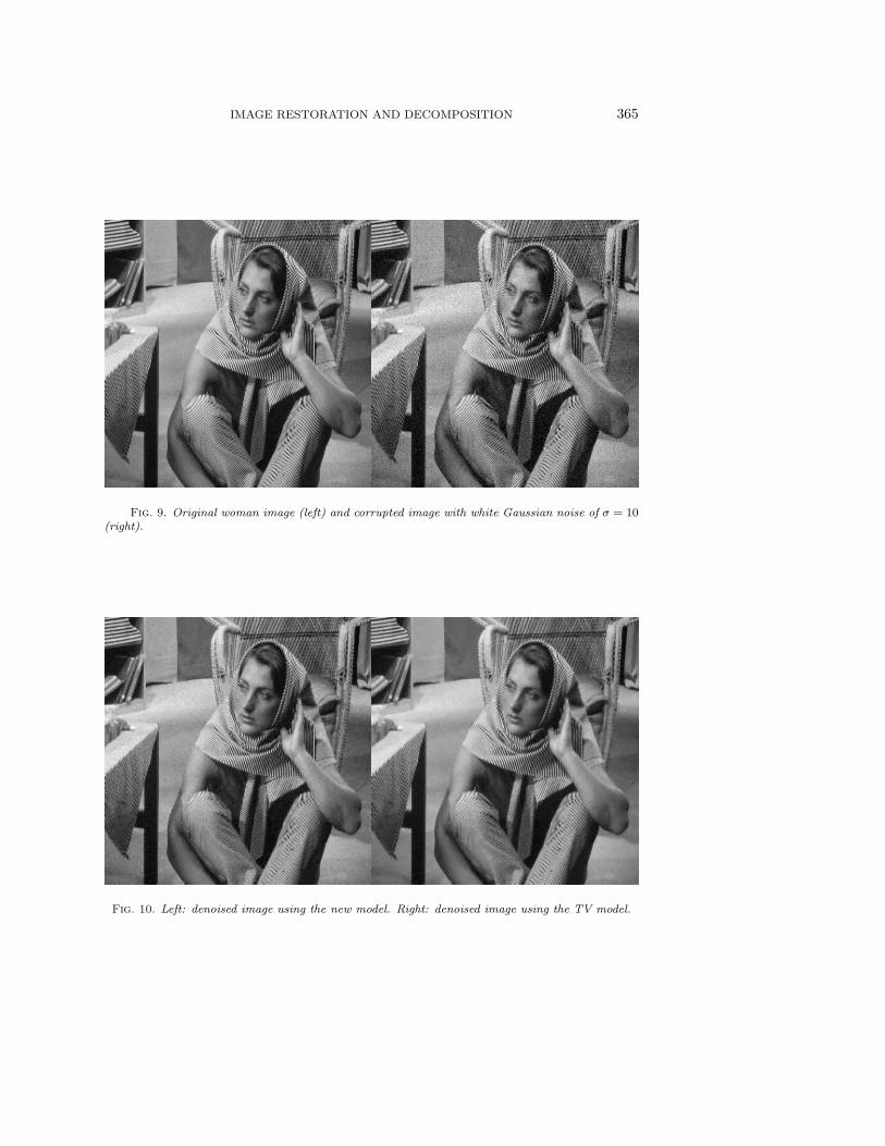
IMAGE RESTORATION AND DECOMPOSITION 365
Fig. 9. Original woman image (left) and corrupted image with white Gaussian noise of σ = 10(right).
Fig. 10. Left: denoised image using the new model. Right: denoised image using the TV model.

366 STANLEY OSHER, ANDRES SOLE, AND LUMINITA VESE
Fig. 11. Zoom of a textured zone, from left to right, top to bottom: original, noisy, denoisedwith the new model, denoised with the TV model.
Fig. 12. Original image (left) and the corrupted image (Gaussian blur of σ = 3 plus additiveGaussian noise of σ = 1).

IMAGE RESTORATION AND DECOMPOSITION 367
Fig. 13. Restoration using the proposed model (left) and the TV model (right).
Fig. 14. Original image (left) and the corrupted image (Gaussian blur of σ = 4 plus additiveGaussian noise of σ = 1). The values for the PSNR (peak to signal to noise ratio) and the RMSE(root mean square error) are, respectively, PSNR = 21.66dB and RMSE = 0.0826.

368 STANLEY OSHER, ANDRES SOLE, AND LUMINITA VESE
Fig. 15. Restoration using the proposed model (left, PSNR = 24.10dB and RMSE = 0.0624)and the TV model (right, PSNR = 23.98dB and RMSE = 0.0633). Observe that the proposed modelgives a slightly better result (higher PSNR and lower RMSE) than the classical TV model.

IMAGE RESTORATION AND DECOMPOSITION 369
Fig. 16. Decomposition of an image with an object with fractal boundary (corresponding to the“Sierpinsky pentagon”) using the new model. Top: f ; bottom left: u; bottom right: v.
370 STANLEY OSHER, ANDRES SOLE, AND LUMINITA VESE
Acknowledgments. The authors would like to thank A. Marquina, from theUniversity of Valencia, Spain, for providing us the satellite image, and V. Caselles,A. Chambolle, and Y. Meyer for their helpful comments on the first draft of the paper.
REFERENCES
[1] R. Acart and C.R. Vogel, Analysis of bounded variation penalty methods of ill-posed prob-lems, Inverse Problems, 10 (1994), pp. 1217–1229.
[2] F. Andreu, C. Ballester, V. Caselles, and J.M. Mazon, Minimizing total variation flow,C. R. Acad. Sci. Paris Ser. I Math., 331 (2000), pp. 867–872.
[3] J.-F. Aujol, G. Aubert, L. Blanc-Feraud, and A. Chambolle, Image Decomposition: Ap-plication to Textured Images and SAR Images, Rapport de Recherche RR 4704, INRIA,Sophia-Antipolis Cedex, France, 2003.
[4] M. Bertalmio, L. Vese, G. Sapiro, and S. Osher, Simultaneous structure and texture imageinpainting, IEEE Trans. Image Process., to appear.
[5] S. Casadei, S. Mitter, and P. Perona, Boundary detection in piecewise homogeneoustextured images, in Computer Vision—ECCV ’92, Lecture Notes in Comput. Sci. 588,Springer-Verlag, Berlin, 1992, pp. 174–183.
[6] A. Chambolle, An algorithm for total variation minimization and applications, J. Math.Imaging Vision, to appear.
[7] A. Chambolle and P.L. Lions, Image recovery via total variation minimization and relatedproblems, Numer. Math., 76 (1997), pp. 167–188.
[8] R. Dautray and J.-L. Lions, Mathematical Analysis and Numerical Methods for Science andTechnology, Vol. 2, Functional and Variational Methods, Springer-Verlag, Berlin, 1988.
[9] Y. Ekeland and R. Temam, Analyse Convexe et Problemes Variationnels, Dunod, Gauthier-Villars, Paris, 1974.
[10] L.C. Evans, Partial Differential Equations, Grad. Stud. Math. 19, AMS, Providence, RI, 1998.[11] J.B. Greer and A.L. Bertozzi, H1 Solutions of a Class of Fourth Order Nonlinear Equations
for Image Processing, UCLA CAM Report 03-11, UCLA, Los Angeles, CA, 2003.[12] M. Lysaker, A. Lundervold, and X.-C. Tai, Noise Removal Using Fourth-Order Partial
Differential Equations with Applications to Medical Magnetic Resonance Images in Spaceand Time, UCLA CAM Report 02-44, UCLA, Los Angeles, CA, 2002.
[13] F. Malgouyres, Mathematical analysis of a model which combines total variation and waveletfor image restoration, J. Information Processes, 2 (2002), pp. 1–10.
[14] F. Malgouyres, Minimizing the total variation under a general convex constraint for imagerestoration, IEEE Trans. Image Process., 11 (2002), pp. 1450–1456.
[15] Y. Meyer, Oscillating Patterns in Image Processing and Nonlinear Evolution Equations, Univ.Lecture Ser. 22, AMS, Providence, RI, 2002.
[16] D. Mumford and B. Gidas, Stochastic models for generic images, Quart. Appl. Math., 59(2001), pp. 85–111.
[17] F. Oru, Le role des oscillations dans quelques problemes d’analyse non-lineaire, These, CMLA,ENS-Cachan, Cachan cedex, France, 1998.
[18] L. Rudin and S. Osher, Total variation based image restoration with free local constraints, inProceedings of the IEEE ICIP 1994, Vol. I, Austin, TX, pp. 31–35.
[19] L. Rudin, S. Osher, and E. Fatemi, Nonlinear total variation based noise removal algorithms,Phys. D, 60 (1992), pp. 259–268.
[20] L. Vese, A study in the BV space of a denoising-deblurring variational problem, Appl. Math.Optim., 44 (2001), pp. 131–161.
[21] L. Vese and S. Osher, Modeling textures with total variation minimization and oscillatingpatterns in image processing, J. Sci. Comput., to appear.
[22] L. Vese and S. Osher, Image denoising and decomposition with total variation minimizationand oscillatory functions, J. Math. Imaging Vision, to appear.
[23] S.C. Zhu, Y.N. Wu, and D. Mumford, Filters, random fields and maximum entropy(FRAME): Towards a unified theory for texture modeling, Internat. J. Computer Vision,27 (1998), pp. 107–126.
[24] S.C. Zhu, Y.N. Wu, and D. Mumford, Minimax entropy principle and its application totexture modeling, Neural Computation, 9 (1997), pp. 1627–1660.