iii. multi-dimensional random variables and application in vector quantization
TRANSCRIPT

III. Multi-Dimensional Random Variables and Application in Vector Quantization

© Tallal Elshabrawy 2

© Tallal Elshabrawy 3

© Tallal Elshabrawy 4

© Tallal Elshabrawy 5

© Tallal Elshabrawy 6
© Tallal Elshabrawy 7
Karhunen-Loeve Decomposition
v1
u2 X=[X1, X2]
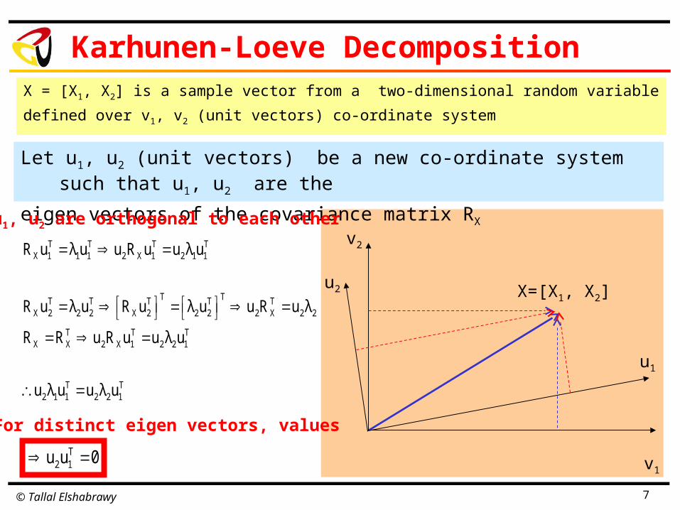
X = [X1, X2] is a sample vector from a two-dimensional random variable
defined over v1, v2 (unit vectors) co-ordinate system
Let u1, u2 (unit vectors) be a new co-ordinate system such that u1, u2 are the
eigen vectors of the covariance matrix RX
u1
v2
u1, u2 are orthogonal to each otherT T T T
X 1 1 1 2 X 1 2 1 1
T TT T T T TX 2 2 2 X 2 2 2 2 X 2 2
T T TX X 2 X 1 2 2 1
T T2 1 1 2 2 1
R u λ u u R u u λ u
R u λ u R u λ u u R u λ
R R u R u u λ u
u λ u u λ u
T2 1u u 0
For distinct eigen vectors, values
© Tallal Elshabrawy 8
Karhunen-Loeve Decomposition
v1
u2 X=[X1, X2]
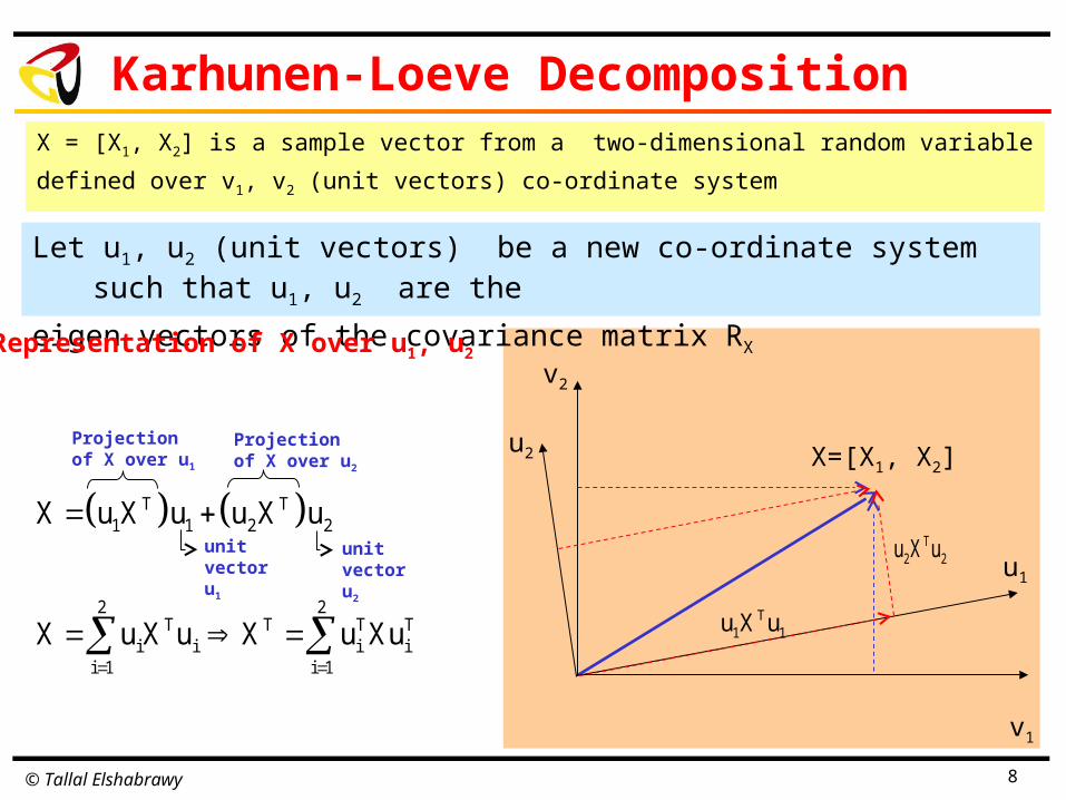
X = [X1, X2] is a sample vector from a two-dimensional random variable
defined over v1, v2 (unit vectors) co-ordinate system
Let u1, u2 (unit vectors) be a new co-ordinate system such that u1, u2 are the
eigen vectors of the covariance matrix RX
u1
T1 1u X u
T2 2u X u
v2
Representation of X over u1, u2
T T1 1 2 2
2 2T T T T
i i i ii 1 i 1
X u X u u X u
X u X u X u Xu
Projection of X over u1
unit vector u1
Projection of X over u2
unit vector u2

© Tallal Elshabrawy 9
Karhunen-Loeve Decomposition
v1
u2 X=[X1, X2]
X = [X1, X2] is a sample vector from a two-dimensional random variable
defined over v1, v2 (unit vectors) co-ordinate system
Let u1, u2 (unit vectors) be a new co-ordinate system such that u1, u2 are the
eigen vectors of the covariance matrix RX
u1
T1 1u X u
T2 2u X u
v2
Diagonalization of RX
2T T T
X X i ii 1
2T T T
X X i ii 1
T TX i i i
2T T T
X i i ii 1
R X R u Xu
R X R u Xu
R u λ u
R X λ u Xu

© Tallal Elshabrawy 10
Karhunen-Loeve Decomposition
v1
u2 X=[X1, X2]
X = [X1, X2] is a sample vector from a two-dimensional random variable
defined over v1, v2 (unit vectors) co-ordinate system
Let u1, u2 (unit vectors) be a new co-ordinate system such that u1, u2 are the
eigen vectors of the covariance matrix RX
u1
T1 1u X u
T2 2u X u
v2
T Ti i
2T T T
X i i ii 1
2T T T
X i i ii 1
T TX 1 1 1 2 2 2
Xu u X
R X λ u u X
R X λ u u X
R λ u u λ u u
Diagonalization of RX

© Tallal Elshabrawy 11
Karhunen-Loeve Decomposition
v1
u2 X=[X1, X2]
X = [X1, X2] is a sample vector from a two-dimensional random variable
defined over v1, v2 (unit vectors) co-ordinate system
Let u1, u2 (unit vectors) be a new co-ordinate system such that u1, u2 are the
eigen vectors of the covariance matrix RX
u1
T1 1u X u
T2 2u X u
v2
T TX 1 1 1 2 2 2
1 1T TX 1 2
2 2
TX
R u λ u u λ u
λ 0 uR u u
0 λ u
R U ΛU
1 11 12 2 21 22u u u , u u u
1 11 12
2 21 22
u u uU
u u u
1
2
λ 0Λ
0 λ
Diagonalization of RX

© Tallal Elshabrawy 12
K-L Transformation of 2-D Random Variable
v1
u2X
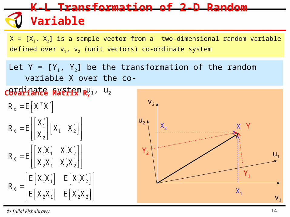
X = [X1, X2] is a sample vector from a two-dimensional random variable
defined over v1, v2 (unit vectors) co-ordinate system
Let Y = [Y1, Y2] be the transformation of the random variable X over the co-
ordinate system u1, u2
u1
v2
X1
X2 Y
Y1
Y2

© Tallal Elshabrawy 13
K-L Transformation of 2-D Random Variable
v1
u2X
X = [X1, X2] is a sample vector from a two-dimensional random variable
defined over v1, v2 (unit vectors) co-ordinate system
Let Y = [Y1, Y2] be the transformation of the random variable X over the co-
ordinate system u1, u2
u1
v2
X1
X2 Y
Y1
Y2 1 2
'x 1 2 x xX X m X X m m
T1 1
T2 2
T T T1 2 1 2
Y Xu
Y Xu
Y Y Y X u u XU
1 2
'Y 1 2 Y YY Y m Y Y m m
Define
Define E[X1] E[X2]
E[Y1] E[Y2]
© Tallal Elshabrawy 14
K-L Transformation of 2-D Random Variable
v1
u2X
X = [X1, X2] is a sample vector from a two-dimensional random variable
defined over v1, v2 (unit vectors) co-ordinate system
Let Y = [Y1, Y2] be the transformation of the random variable X over the co-
ordinate system u1, u2
u1
v2
X1
X2 Y
Y1
Y2
'T 'X
'' '1
X 1 2'2
' ' ' '1 1 1 2
X ' ' ' '2 1 2 2
' ' ' '1 1 1 2
X ' ' ' '2 1 2 2
R E X X
XR E X X
X
X X X XR E
X X X X
E X X E X XR
E X X E X X
Covariance Matrix RX

© Tallal Elshabrawy 15
K-L Transformation of 2-D Random Variable
v1
u2X
X = [X1, X2] is a sample vector from a two-dimensional random variable
defined over v1, v2 (unit vectors) co-ordinate system
Let Y = [Y1, Y2] be the transformation of the random variable X over the co-
ordinate system u1, u2
u1
v2
X1
X2 Y
Y1
Y2
'T 'Y
Y 1 2
T TY 1 2
T TY 1 2
T TY X 1 2
TY X
R E Y Y
m E Y E Y
m E Xu E Xu
m E X u E X u
m m u u
m m U
Covariance Matrix RY

© Tallal Elshabrawy 16
K-L Transformation of 2-D Random Variable
v1
u2X
X = [X1, X2] is a sample vector from a two-dimensional random variable
defined over v1, v2 (unit vectors) co-ordinate system
Let Y = [Y1, Y2] be the transformation of the random variable X over the co-
ordinate system u1, u2
u1
v2
X1
X2 Y
Y1
Y2
' T TY X
' ' T
Y Y m XU m U
Y X U
'
'
'T 'Y
T' T ' TY
T ' TY
T ' T TY X
R E Y Y
R E X U X U
R E UX X U
R UE X X U UR U
Covariance Matrix RY

© Tallal Elshabrawy 17
K-L Transformation of 2-D Random Variable
v1
u2X
X = [X1, X2] is a sample vector from a two-dimensional random variable
defined over v1, v2 (unit vectors) co-ordinate system
Let Y = [Y1, Y2] be the transformation of the random variable X over the co-
ordinate system u1, u2
u1
v2
X1
X2 Y
Y1
Y2
TY X
TX
T TY
T
1Y
2
R UR U
R U ΛU
R U U ΛU U
UU I
λ 0R Λ
0 λ
Y1 and Y2 are UNCORRELATED
Covariance Matrix RY

© Tallal Elshabrawy 18
K-L Transformation of 2-D Random Variable
Therefore using principle component analysis, it is possible to transform a random variable X with components X1 and X2 that are correlated into another random variable Y whose components Y1 and Y2 are uncorrelated
v1
u2X
u1
v2
X1
X2 Y
Y1
Y2
TY X
Y
m m U
R Λ
u1, u2 are eigen vectors of RX
λ1, λ2 are eigen values of RX
1
2
uU
u
1
2
λ 0Λ
0 λ

© Tallal Elshabrawy 19
Two-Dimensional Gaussian Distribution
In the previous slides, we have talked about the transformed random variable Y whose components are uncorrelated and have mean mY
and covariance matrix RY. What would be the distribution of Y. Well this depends on what is the distribution of X
Generally X and Y do not follow a Gaussian distribution. However, if X is a two-dimensional Gaussian distribution then Y as well would be a two-dimensional Gaussian distribution

© Tallal Elshabrawy 20
Two-Dimensional Gaussian Distribution
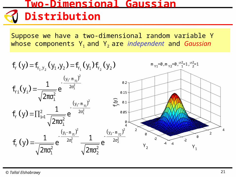
Suppose we have a two-dimensional random variable Y whose components Y1 and Y2 are independent and Gaussian
1 2 1 2Y Y ,Y 1 2 Y 1 Y 2f y f y , y f y f y
2
i yi2i
y m
2σYi i 2
i
1f y e
2πσ
-3 -2 -1 0 1 2 30
0.02
0.04
0.06
0.08
0.1
0.12
0.14
0.16
Y1
f Y1(y
1)
mY1
=0,12=1
© Tallal Elshabrawy 21
Two-Dimensional Gaussian Distribution
Suppose we have a two-dimensional random variable Y whose components Y1 and Y2 are independent and Gaussian
1 2 1 2Y Y ,Y 1 2 Y 1 Y 2f y f y , y f y f y
2
i yi2i
y m
2σYi i 2
i
1f y e
2πσ
2
i yi2i
y m
2σ2Y i 1 2
i
1f y e
2πσ
2 2
1 y 2 y1 22 21 2
y m y m
2σ 2σY 2 2
1 2
1 1f y e e
2πσ 2πσ
-4-2
02
4
-4-2
02
40
0.05
0.1
0.15
0.2
Y1
mY1
=0, mY2
=0, 12=1,
22=1
Y2
f y(y)

© Tallal Elshabrawy 22
Two-Dimensional Gaussian Distribution
Suppose we have a two-dimensional random variable Y whose components Y1 and Y2 are independent and Gaussian
1 2 1 2Y Y ,Y 1 2 Y 1 Y 2f y f y , y f y f y
2
i yi2i
y m
2σYi i 2
i
1f y e
2πσ
2
i yi2i
y m
2σ2Y i 1 2
i
1f y e
2πσ
2 2
1 y 2 y1 22 21 2
y m y m
2σ 2σY 2 2
1 2
1 1f y e e
2πσ 2πσ
mY1
=0, mY2
=0, 12=1,
22=1
Y1
Y2
-3 -2 -1 0 1 2 3-3
-2
-1
0
1
2
3

© Tallal Elshabrawy 23
Two-Dimensional Gaussian Distribution
Suppose we have a two-dimensional random variable Y whose components Y1 and Y2 are independent and Gaussian
2 2
2 y 2 y2 22 22 2
y m y m1
2 σ σ
Y 2 21 2
1f y e
2π σ σ
This formula is valid for any multi-dimensional Gaussian random variable whether its components are correlated or not
2 1
2 21 2Y 1 2 Y2
2
σ 0R σ σ det R
0 σ
2 ' '2 '21' 1 'T ' ' 1 1 2
Y 1 2 2 2'1 22
22
10
σ Y Y YY R Y Y Y
1 σ σY0
σ
' 1 'TY
1Y R Y
2Y 1
2Y
1f y e
2π det R

© Tallal Elshabrawy 24
Two-Dimensional Gaussian Distribution
-4-2
02
4
-4
-2
0
2
40
0.05
0.1
0.15
0.2
Y1
mY1
=0, mY2
=0, 12=1,
22=1,
Y2
f Y(y
)
-4-2
02
4
-4
-2
0
2
40
0.05
0.1
0.15
0.2
Y1
mY1
=0, mY2
=0, 12=1,
22=1,
Y2
f Y(y
)
-4-2
02
4
-4
-2
0
2
40
0.05
0.1
0.15
0.2
0.25
Y1
mY1
=0, mY2
=0, 12=1,
22=1,
Y2
f Y(y
)
-4-2
02
4
-4
-2
0
2
40
0.5
1
1.5
Y1
mY1
=0, mY2
=0, 12=1,
22=1,
Y2
f Y(y
)
Y
1 0.25R
0.25 1
Y
1 0.5R
0.5 1
Y
1 0.75R
0.75 1
Y
1 0.99R
0.99 1

© Tallal Elshabrawy 25
Two-Dimensional Gaussian Distribution
Y1
Y2
mY1
=0, mY2
=0, 12=1,
22=1,
-3 -2 -1 0 1 2 3-3
-2
-1
0
1
2
3
Y1
Y2
mY1
=0, mY2
=0, 12=1,
22=1,
-3 -2 -1 0 1 2 3-3
-2
-1
0
1
2
3
Y1
Y2
mY1
=0, mY2
=0, 12=1,
22=1,
-3 -2 -1 0 1 2 3-3
-2
-1
0
1
2
3
Y1
Y2
mY1
=0, mY2
=0, 12=1,
22=1,
-3 -2 -1 0 1 2 3-3
-2
-1
0
1
2
3
Y
1 0.25R
0.25 1
Y
1 0.5R
0.5 1
Y
1 0.75R
0.75 1
Y
1 0.99R
0.99 1

© Tallal Elshabrawy 26
Two-Dimensional Gaussian Distribution
-4-2
02
4
-4
-2
0
2
40
0.05
0.1
0.15
0.2
Y1
mY1
=0, mY2
=0, 12=1,
22=1,
Y2
f Y(y
)
-4-2
02
4
-4
-2
0
2
40
0.05
0.1
0.15
0.2
Y1
mY1
=0, mY2
=0, 12=1,
22=1,
Y2
f Y(y
)
-4-2
02
4
-4
-2
0
2
40
0.05
0.1
0.15
0.2
0.25
Y1
mY1
=0, mY2
=0, 12=1,
22=1,
Y2
f Y(y
)
-4-2
02
4
-4
-2
0
2
40
0.5
1
1.5
Y1
mY1
=0, mY2
=0, 12=1,
22=1,
Y2
f Y(y
)
Y
1 0.25R
0.25 1
Y
1 0.5R
0.5 1
Y
1 0.75R
0.75 1
Y
1 0.99R
0.99 1

© Tallal Elshabrawy 27
Two-Dimensional Gaussian Distribution
Y1
Y2
mY1
=0, mY2
=0, 12=1,
22=1,
-3 -2 -1 0 1 2 3-3
-2
-1
0
1
2
3
Y1
Y2
mY1
=0, mY2
=0, 12=1,
22=1,
-3 -2 -1 0 1 2 3-3
-2
-1
0
1
2
3
Y1
Y2
mY1
=0, mY2
=0, 12=1,
22=1,
-3 -2 -1 0 1 2 3-3
-2
-1
0
1
2
3
Y1
Y2
mY1
=0, mY2
=0, 12=1,
22=1,
-3 -2 -1 0 1 2 3-3
-2
-1
0
1
2
3
Y
1 0.25R
0.25 1
Y
1 0.5R
0.5 1
Y
1 0.75R
0.75 1
Y
1 0.99R
0.99 1

© Tallal Elshabrawy 28
Two-Dimensional Gaussian Distribution
Y1
Y2
mY1
=0, mY2
=0, 12=1.5,
22=0.5,
-3 -2 -1 0 1 2 3-3
-2
-1
0
1
2
3
Y
1.5 0R
0 0.5

© Tallal Elshabrawy 29
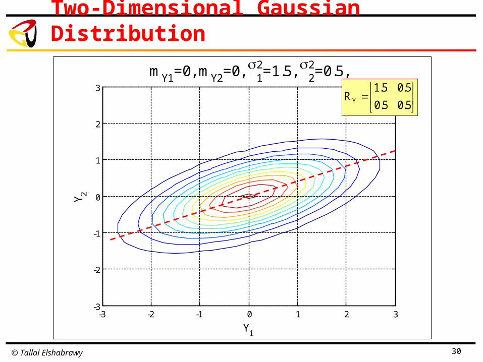
Two-Dimensional Gaussian Distribution
Y1
Y2
mY1
=0, mY2
=0, 12=1.5,
22=0.5,
-3 -2 -1 0 1 2 3-3
-2
-1
0
1
2
3
Y
1.5 0.25R
0.25 0.5
© Tallal Elshabrawy 30
Two-Dimensional Gaussian Distribution
Y1
Y2
mY1
=0, mY2
=0, 12=1.5,
22=0.5,
-3 -2 -1 0 1 2 3-3
-2
-1
0
1
2
3
Y
1.5 0.5R
0.5 0.5
© Tallal Elshabrawy 31
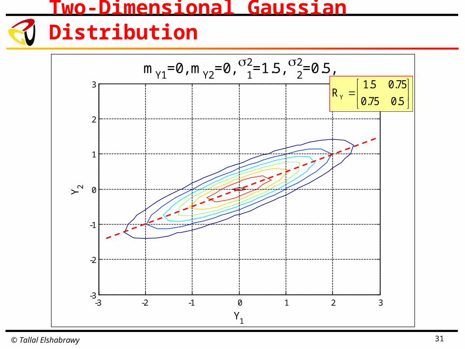
Two-Dimensional Gaussian Distribution
Y1
Y2
mY1
=0, mY2
=0, 12=1.5,
22=0.5,
-3 -2 -1 0 1 2 3-3
-2
-1
0
1
2
3
Y
1.5 0.75R
0.75 0.5

© Tallal Elshabrawy 32
Two-Dimensional Gaussian Distribution
Y1
Y2
mY1
=0, mY2
=0, 12=1.9,
22=0.1,
-3 -2 -1 0 1 2 3-3
-2
-1
0
1
2
3
Y
1.9 0R
0 0.1

© Tallal Elshabrawy 33
Two-Dimensional Gaussian Distribution
Y1
Y2
mY1
=0, mY2
=0, 12=1.9,
22=0.1,
-3 -2 -1 0 1 2 3-3
-2
-1
0
1
2
3
Y
1.9 0.25R
0.25 0.1

© Tallal Elshabrawy 34
Two-Dimensional Gaussian Distribution
Y
1 0.5R
0.5 1

© Tallal Elshabrawy 35
Two-Dimensional Gaussian Distribution
Y1
Y2
mY1
=0, mY2
=0, 12=1,
22=1,
-3 -2 -1 0 1 2 3-3
-2
-1
0
1
2
3Y
1 0.5R
0.5 1
More Energy
More Energy
Less Energy
Less Energy
Y1 and Y2 Correlated

© Tallal Elshabrawy 36
Two-Dimensional Gaussian Distribution
Y1
Y2
mY1
=0, mY2
=0, 12=1,
22=1,
-3 -2 -1 0 1 2 3-3
-2
-1
0
1
2
3Y
1 0.5R
0.5 1
Equal
Energy
Equal Energy
Equal Energy
Equal Energy
By rotating the axis, the resultant transformed random variables are uncorrelated