iii assessment on water quality and biodiversity

iii

ASSESSMENT ON WATER QUALITY AND BIODIVERSITY WITHIN

SUNGAI BATU PAHAT

NURHIDAYAH BINTI HAMZAH

A project report submitted in partial fulfilment of the

requirements for the award of the degree of

Master of Engineering (Civil – Environmental Management)

Faculty of Civil Engineering

Universiti Teknologi Malaysia

JUNE, 2007

v

Hanya yang tHanya yang tHanya yang tHanya yang teristimewa buateristimewa buateristimewa buateristimewa buat

Ayahanda Hamzah bin Rostam

Bonda Kamaliah binti Shukor

Abang-abang;

Mohd Azril Fariz

Mohd Khuzairi

Mohd Hafeez Azad

Adik-adik;

Mohd Zul Iqbal

Mohd Irfan

Mohd Sufi Akhbar

&

Untuk iUntuk iUntuk iUntuk innnnsan tersayangsan tersayangsan tersayangsan tersayang

Mahzan bin Manan

vi

ACKNOWLEDGEMENT

“In the name of God, the most gracious, the most compassionate”

First and foremost, a very special thanks and appreciation to my supervisor, Dr Johan

Sohaili for being the most understanding, helpful and patient lecturer I have come to

know. I would also like to express my deep gratitude to my co-supervisor, PM. Dr.

Mohd Ismid bin Mohd Said for his valuable time, guidance and encouragement

throughout the course of this research.

Not forgetting may lovely family that always by my side to support me all the way.

Finally, I wish to extend my heartfelt thanks to all environmental laboratories

technicians for their timely support during my survey.

Last but not least, I also owes special thanks to my friends, who have always been

there for me and extended every possible support during this research.

vii

ABSTRAK

Sungai Batu Pahat sedang mengalami kemerosotan kualiti air dan banyak tumbuhan disekitarnya telah musnah. Kajian ini tertumpu kepada penentuan status Sungai Batu Pahat berdasarkan analisis kualiti air dan kepelbagaian biologi secara kualitatif dan kuantitatif. Terdapat enam parameter utama yang diambilkira dalam kajian ini iaitu oksigen terlarut (DO), permintaan oksigen biokimia (BOD), permintaan oksigen kimia (COD), nitrogen ammonia (NH3-N), pepejal terampai (SS) dan pH. Manakala parameter biologi pula terdiri daripada ikan, zooplankton, phytoplankton, macrobenthos dan tumbuhan tebing sungai. Kualiti air yang didapati menunjukkan tahap yang seragam dengan kualiti air yang kurang memuaskan di mana berdasarkan DOE-WQI, di hilir dan hulu sungai, data menunjukkan kualiti air di kelas III tetapi menurun ke kelas IV di tengah sungai. Ini mungkin disebabkan oleh aktiviti guna tanah di kawasan tebing sungai seperti aktiviti kuari dan penempatan penduduk. Jika dilihat pada data kepelbagaian biologi, terdapat banyak anak ikan yang mempunyai nilai komersial yang tinggi yang masih hidup kerana kepekatan DO yang didapati melebihi 2 mg/L dan juga kualiti makanan yang tinggi yang diperolehi dari tumbuhan di tebing sungai. Secara umumnya, taburan hidupan plankton dan macroinvertebrata di kawasan kajian sangat dipengaruhi oleh pasang- surut air dan juga pokok bakau. Kepelbagaian biologi didapati tertumpu di kawasan hulu sungai dan bilangannya berkurang di hilir dan tengah sungai kemungkinan disebabkan oleh aktiviti guna tanah yang aktif. Kebanyakan kepelbagaian biologi yang dijumpai adalah dari spesis yang tidak sensitif pada kepekatan oksigen terlarut dan pH yang rendah. Kesan ketara akibat kemerosotan kualiti air boleh dilihat pada habitat macrobenthos yang dijumpai sewaktu kajian dilakukan di mana, macrobenthos hampir pupus dan hanya yang tinggal adalah dari spesis yang tidak sensitif kepada pencemaran. Walaubagaimanapun, terdapat juga banyak kepelbagaian biologi (zooplankton dan phytoplankton) yang sensitif kepada pencemaran di kawasan kajian dan ini memberi erti bahawa Sungai Batu Pahat masih lagi mampu untuk menampung hidupan aquatik kerana ia menyediakan tempat tinggal, tempat membiak dan makanan yang berkualiti tinggi walaupun kualiti air menunjukkan sebaliknya.

viii

ABSTRACT

Sungai Batu Pahat is undergoing poor condition in term of water quality and

riverbank vegetation. This study was focus on determining the status of Sungai Batu Pahat due to quantitative and qualitative of water quality and biodiversity analysis. There are six major water quality parameter that considered in this study which are dissolved oxygen (DO), biochemical oxygen demand (BOD), chemical oxygen demand (COD), ammoniacal nitrogen (NH3-N), suspended solid (SS) and pH. Biodiversity parameter consists of fish, zooplankton, phytoplankton, macrobenthos and riverbank vegetation. Water quality shows a consistent level with low quality of water which is class III at upstream and downstream but dropped to class IV at middle stream according to DOE-WQI. This could be a consequence of riverbank landuse activities such as quarry and settlement. If based on biodiversity data, the juvenile commercial fish still exist correspond to >2 mg/L of DO concentration and quality food supply from riverbank vegetation. Generally, the distribution of planktonic life and macroinvertebrates within study area was tidal and mangrove dependent. Biodiversity was found abundance at downstream and present with low number and species at upstream and downstream probably because lands use activities. Biodiversity that mostly found within study area is tolerant species to low dissolved oxygen concentration and pH. The impact of water quality can clearly be seen with respect to macrobenthos habitat. Macrobenthos almost disappeared during study event and only tolerant species was present. However, the abundance of high demanding biodiversity (zooplankton and phytoplankton) giving the good result that Sungai Batu Pahat still can support aquatic life due in term of shelter, feeding and breeding area even, the quality of water shows otherwise.

ix

CONTENT

CHAPTER TITLE PAGE

DECLARATION ii

DEDICATION iii

ACKNOWLEDGEMENTS iv

ABSTRAK v

ABSTRACT vi

CONTENTS vii

LIST OF TABLES xi

LIST OF FIGURES xiii

LIST OF SYMBOLS xvii

I INTRODUCTION 1

1.1 Introduction 1

1.2 Site Description 2

1.3 Objective of Study 3

1.4 Scope of Study 3

1.5 Needs of Study 4

x

II LITERATURE REVIEW 5

2.1 Overview 5

2.2 Study Background 6

2.3 Sources of River Water Pollution 8

2.4.1 Natural Factor 8

2.4.2 Human Factor 9

2.4 Effect of Land use Activity 10

2.4.1 Agricultural Activity 10

2.4.2 Settlements Activity 11

2.5 Physico-chemical Parameter 12

2.5.1 Dissolve Oxygen (DO) 12

2.5.2 Biochemical Oxygen Demand (BOD) 13

2.5.3 Chemical Oxygen Demand (COD) 14

2.5.4 Suspended Solids (SS) 15

2.5.5 Ammoniacal Nitrogen (NH3-N) 16

2.5.6 Acidity and Alkalinity (pH) 17

2.6 Biological Parameter 18

2.6.1 Fish 18

2.6.2 Zooplankton 20

2.6.3 Phytoplankton 21

2.6.4 Benthos 22

2.6.5 Mangrove 24

2.7 River Classification 27

2.8 River Classification Based on Biological Indicator 30

III METHODOLOGY 32

3.1 Introduction 32

3.2 Literature Review 32

3.3 Determine the Parameter Involved 33

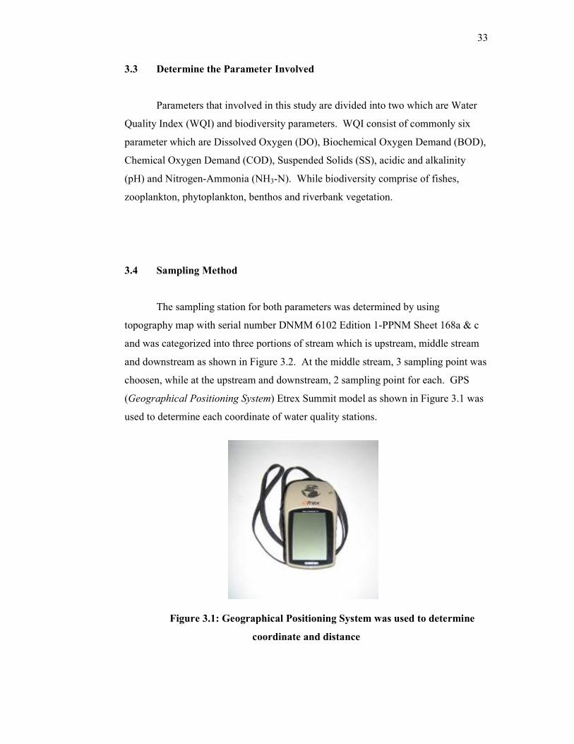
3.4 Sampling Method 33

xi

3.4.1 Water Quality Sampling 37

3.4.2 Fisheries Sampling 38

3.4.3 Phytoplankton 39

3.4.4 Zooplankton 40

3.4.5 Macrobenthos 41

3.4.6 Riverbank Vegetation Analysis 42

3.5 Chemical Analysis 42

3.5.1 Concentration Measurement of Biochemical

Oxygen Demand (BOD5) 43

3.5.2 Concentration Measurement Of Chemical Oxygen

Demand (COD) 43

3.5.3 Concentration Measurement Of Nitrogen-Ammonia

(NH3-N) 43

3.5.4 Measurement of Suspended Solids (SS) 43

3.6 Data Analysis 43

IV RESULT AND ANALYSIS 45

4.1 Introduction 45

4.2 Land Use Analysis 46

4.2.1 Residential 48

4.2.2 Agricultural and Farming 49

4.2.3 Commercial 50

4.2.4 Industrial 51

4.3 Water Quality Analysis 52

4.4 Water Quality Index Analysis 55

4.5 Water Quality Parameter Analysis 58

4.5.1 Dissolved Oxygen 58

4.5.2 Biochemical Oxygen Demand 60

4.5.3 Chemical Oxygen Demand 61

4.5.4 Ammoniacal Nitrogen 62

4.5.5 Suspended Solids 64

4.5.6 pH 65

xii

4.6 Biological Analysis 67

4.6.1 Riverbank Vegetation Result 67

4.6.2 Fish Result 69

4.7 Phytoplankton Analysis 74

4.7.1 Distribution Pattern of Phytoplankton

Due to Riverbank Vegetation 76


Due to Dissolved Oxygen 78


Due to pH 79

4.8 Zooplankton Analysis 79

4.8.1 Distribution Pattern of Zooplankton





Due to pH 85

4.9 Macrobenthos Analysis 85

4.9.1 Distribution Pattern of Macobenthos


4.9.2 Distribution Pattern of Macrobenthos


4.9.3 Distribution Pattern of Macrobenthos Due to pH 89

V CONCLUSION 90

5.1 Conclusion 90

5.2 Recommendation 91

REFERENCES 93

APPENDIX 113

xiii

LIST OF TABLES

TABLE TITLE PAGE

2.1

2.2

2.3

2.4

2.5

4.1

4.2

4.3

4.4

4.5

4.6

4.7

4.8

4.9

4.10

4.11

4.12

4.13

4.14

4.15

4.16

4.17

Water Quality Index (WQI)

Department of Enviroments’ Water Quality Index Standard

Parameter Subindex DOE-WQI

Interim National Water Quality Standard for Malaysia

(INWQS) with related of water quality parameter

Water Quality Determination based on Shannon-Weiner

Diversity Index

Distribution of exiting land use in Batu Pahat

List of subdistricts in Batu Pahat

Water quality parameter result during high tide

Water quality parameter result during low tide

Water quality subindex parameters result during high tide

Water quality subindex parameters result during low tide

Riverbank vegetation that mostly found at Sungai Batu

Pahat

Number of fishermen according to district

Fish species found in Sungai Batu Pahat

Range of fish species length

Phytoplankton taxa during high tide

Phytoplankton taxa during low tide

Phytoplankton taxa as compared to DO concentration

Phytoplankton taxa as compared to pH

Zooplankton during high tide in unit ind/m3

Zooplankton during low tide in unit ind/m3

Zooplankton numbers as compared to DO concentration

27

27

28

29

31

46

47

53

53

54

54

68

70

72

72

74

75

78

79

80

81

84

xiv

4.18

4.19

4.20

4.21

4.22

Zooplankton numbers as compared to pH

Benthic macroinvetebrates within study area during high

tide

Benthic macroinvetebrates within study area during low

tide

Numbers of macrobenthos as compared to DO

concentration

Numbers of macrobenthos as compared to pH

85

86

86

88

89

xv

LIST OF FIGURES

FIGURE TITLE PAGE

1.1

2.1

2.2

3.1

3.2

3.3

3.4

3.5

3.6

3.7

Major land use that had been identified around Sungai Batu

Pahat

Common crab in mangrove swamps-Porcelain Fiddler(Uca

annulipes)

Mangrove roots that act as home and hiding place for

juvenile fish against predator

Geographical Positioning System was used to determine

coordinate and distance

Portions of Water Quality Sampling Station at Sungai Batu

Pahat

Upstream of Sungai Batu Pahat. Patches of Nypa habitat

are abundance at the upstream because of low salinity water

compared to seaward. Water seems to be cleaner from

turbidity

A lot of shipping activity occurred at the middle stream of

the estuary, resulting disturbance of biodiversity and

riverbank vegetation as well as water quality depletion

Downstream of Sungai Batu Pahat is adjacent to coastal

water that have wide opening. At downstream, the land are

fully covered by riverbank vegetation especially mangrove

in order to protect against tsunami

Sungai Batu Pahat during high tide. Fresh water from the

river is mixing with coastal water and abundance of fish

will take this opportunity to breed at vegetations’ roots

During low tide, the roots of vegetation were clearly seen

2

24

25

33

34

35

35

36

36

xvi

3.8

3.9

3.10

3.11

3.12

3.13

3.14

4.1

4.2

4.3

4.4

4.5

4.6

4.7

and this is the time for adult fish go to open sea because,

water from estuary was flowing seaward during this period

Multi-Parameter Analyzer-Consort C535 that had been

used to determine pH level on surface water of Sungai Batu

Pahat

55-YSI Dissolved Oxygen Meter was used in order to get

dissolved oxygen concentration in unit mg/L on surface

water

Cast net had been used thirty (30) times for fish sampling.

Trammel net was used for five (5) times at certain part of

the river where drift net using is allowed

Water sampling using Van Dorn Sampler in order to

identify phytoplankton assemblages

Zooplankton had been caught using plankton net at 0.5m

depth from the water surface

Ekman grab sampler that used to identify benthic animals

with 500µm Endecott sieve on board

Squatter area located by the river with improper sewage

treatment and solid waste collection system

Dumping area that made by local resident and resulting

poor view and bad odour

Trade activities along Sungai Batu Pahat that trades goods

and groceries such as logs and timbers

Busy quarry activities during day time along Jalan Minyak

Beku closed to Sungai Batu Pahat

Trend of water quality from upstream towards downstream

during high tide and low tide where water quality was

dropped to class IV at middle stream associated with nine

potential tributaries that contribute pollutant to estuaries

Rubbish that floating on surface water of Sungai Batu Pahat

which carried by flow during ebbing time from upstream of

the estuaries to coastal area

The fluctuation of dissolved oxygen concentration during

37

37

38

38

39

39

40

41

48

49

50

52

55

57

xvii

4.8

4.9

4.10

4.11

4.12

4.13

4.14

4.15

4.16

4.17

high tide and low tide with respect to distance which is

increased towards downstream

For both tides, BOD concentration was increased from

upstream and constant as reach at distance 3.21 km to

seawards due to human activities at middle stream and

undisturbed mangrove area at downstream which is known

as abundance organic matter contributor to water bodies

COD concentration that consistent seaward for high tide

because of dilution from coastal water. However, during

low tide, COD was increased at middle stream due to

leaching of organic matter and inorganic matter from

mangrove area, urban area, as well as decaying of aquatic

plants

Ammoniacal nitrogen decreasing seawards for high tide

and low tide due to increasing of dissolved oxygen

concentration

Profile of suspended solids from upstream to downstream

during high tide and low tide which is increased from

upstream to adjacent of coastal water probably because of

bottom sediment disturbance consequence from boats and

ships traffics as well as imported of suspended solids from

mangrove area and Straits of Melaka

pH value within Sungai Batu Pahat that can be concluded

as acidic water because of natural geology and activities at

mangroves’ roots that was identified to lower the pH

Family Ariidae (Catfish) that caught during study event

Percentage of species number found within study area

Distribution pattern of phytoplankton taxa which is slightly

increase towards downstream for high tide and low tide

Zooplankton community distribution along the river

Macrobenthos that found during study event which shows

low diversity during high tide and low tide

58

61

62

63

65

66

70

71

76

82

87

xviii

LIST OF ABBREVIATIONS

APHA

BOD

COD

DO

DOE

FSS

GPS

INWQS

IUCN

MEDS

MPBP

SS

UM

USEPA

VSS

WQI

American Public Health Association

Biochemical Oxygen Demand

Chemical Oxygen Demand

Dissolved Oxygen

Department of Environment

Fixed Suspended Solid

Geographical Positioning System

Interim National Water Quality Standard

International Union for Conservation of

Nature and Natural Resources

Microbial Easily Degradable Substrate

Majlis Perbandaran Batu Pahat

Suspended Solid

Universiti Malaya

United State Environmental Protect Agency

Volatile Suspended Solid

Water Quality Index

xix

LIST OF SYMBOLS

km

mg/L

kg/m3

µm

cm

ind/m3

L

N

E

C

P

H’

J’

D’

sp.

%

°C

CO2

H2O

NO3

O2

NO2-

NH3

H2S

FeS2

PO4

H-NH3

Kilometer

Milligram per liter

Kilogram per cubic meter

Micrometer

Centimeter

Individu per cubic meter

Liter

North

East

Carbon

Phophorus

Shannon-Weiner’s Index

Pielous’s Index

Margalef’s Index

Species

Percentage

Degree Celsius

Carbon Dioxide

Water

Nitrate

Oxygen

Nitrite

Ammonia

Hydrogen Sulfide

Iron Sulfide

Phosphate

Nitric Acid

xx

Fe

Pb

Cu

Cd

Zn

Mn

Hg

Iron

Lead

Copper

Cadmium

Zink

Manganese

Mercury

CHAPTER I

INTRODUCTION

1.1 Introduction

River is one of valuable country asset and need to put more attention to

rehabilitate it from time to time. It is should be well cared and concerned of its

importance without any enforcement. By maintaining and well managing the river,

the aesthetic value may increase as well as rate of country economic generation may

improve tremendously. Mangroves are intertidal marine plants, mostly trees, and

thrive in saline conditions and daily inundation between mean sea level and highest

astronomical tides. Mangroves are not a monophyletic taxonomic unit. Fewer than 22

plant families have developed specialized morphological and physiological

characteristics that characterize mangrove plants, such as buttress trunks and roots

providing support in soft sediments and physiological adaptations for excluding and

expelling salt (Schaffelke et al., 2005).

For swampy area like Sungai Batu Pahat, the mangrove plants require certain

heavy metals as essential nutrients; however an excess in these nutrients may

potentially have adverse, ecotoxicological consequences for mangrove communities.

Each mangrove plant species has specific adaptation systems, which may control

their behavior towards pollutants. A study by previous experiment reveals that in

urban area, there are no obvious differences between samples collected in swamps

located upstream and downstream. (Marchand et al., 2005).

2

1.2 Site Description

The main river in the study area is Sungai Batu Pahat which forms from the

joining of two rivers namely Sungai Simpang Kiri and Sungai Simpang Kanan about

3.5 km northwest of the town of Batu Pahat. From the point where Sungai Simpang

Kiri and Sungai Simpang Kanan joins to form Sungai Batu Pahat, the river flows for

approximately 12 km on a south and southwesterly course before draining into the

straits of Melaka near Tanjung Api and Minyak Beku. A few tributaries which are

connected to the river were identified such as Sungai Peserai, Sungai Benang, Sungai

Gudang, Sungai Kajang, Sungai Tambak and Parit Gantong. Within study area,

there are a lot of land use activities such as urban area, quarry, barter-trade jetties and

pig farm as shown in Figure 1.1.

Market

Quarry

Pig FarmMangroves

Primary forest

Residential, Commercial and Industrial

Agriculture

Legend

Figure 1.1: Major land use that had been identified around Sungai Batu Pahat

(Low, 2007)

3

1.3 Objective of Study

The objectives of this study are;

(i) To determine the trends of water quality of Sungai Batu Pahat as

consequence of land use activities;

(ii) To identify the distribution pattern of planktonic life and

macrobenthos due to dissolved oxygen, pH and riverbank vegetation;

(iii) To identify the status of Sungai Batu Pahat based on water quality and

biodiversity analysis.

1.4 Scope of Study

The boundary of this study is from the upstream of Sungai Batu Pahat (1° 51’

35.2” N, 102° 55’ 23.8” E) to the adjacent coastal water of Sungai Batu Pahat, i.e.

Straits of Melaka (1° 47’ 52.1” N, 102° 53’ 30.1” E ). The considering parameter for

this study are water quality parameters which consist of Dissolve Oxygen (DO),

Biological Oxygen Demand (BOD), Chemical Oxygen Demand (COD), pH (Acidity

and Alkalinity), Suspended Solid (SS) and Ammoniacal Nitrogen (NH3-N), and

biological parameters such as fish, zooplankton, phytoplankton, macrobenthos and

river bank vegetation. The sampling of water quality is taken at seven stations with

six times of frequency for both tides (study period is within August 2006 and

September 2006).

The data of biodiversity quantity in term of zooplankton, phytoplankton and

macrobenthos was taken twice at five stations within August and September, 2006.

Fisheries sampling also was taken twice which two times during high tide and two

times during low tide within study period while riverbank vegetations was measured

once within study period because the condition of river bank vegetation is not change

4

from actual observation. Only the patches of vegetation from both side of the river is

considering in this study.

1.5 Needs of Study

Generally, Water Quality Index (WQI) is used to determine the classification

and pollutant status of particular water bodies. However, rely solely on WQI is not

strong enough to define and justify either the aquatic habitat may survive in the water

bodies or vice versa. Instead of using physicochemical parameters, another strong

influenced factor is via biological survey. Aquatic habitat may have bad impact

causes by deteriorating of water quality. Another reason of fish survival is because

of the existing of feeding and breeding area (riverbank vegetation). Beside, there

would be a Second port development within study area (Mukim Peserai). Therefore,

this study is conducted to determine the existing quality of this river and represent as

a baseline data in order to achieve sustainable development.

CHAPTER II

LITERATURE REVIEW

2.1 Overview

River is one of valuable country asset and need to put more attention to

rehabilitate it from time to time. It is should be well cared and concerned of its

importance without any enforcement. By maintain and well manage the river, the

aesthetic value may increase as well as rate of country economic generation may

improve tremendously.

Mangrove forest was surrounded with looses sediment which receive organic

matter from various sources such as bacteria (Bano et al., 1997), algae, mangrove

litter and human activities (Meziane and Tsuchiya, 2001; Tam et al., 1998). Beside

organic matter, human activities such as urbanization and industrialization also

contribute to abundance of pollutant in mangrove sediment

Organic and inorganic pollution is an environmental problem of worldwide

concern because these substance are indestructible and most of them have toxic

effects on living organisms, including humans when they exceed a certain

concentration (Bahadir et al., 2005; Ghrefat and Yusuf, 2006; Ardebili et al., 2006).

Even at low concentration, the tendency to accumulate in the food chain is high

(Corami et al., 2006).

6

Pollutants released into the environment have been increasing continuously

as a result of industrial activities and technological development, posing a significant

threat to the environment and public health because of their toxicity, accumulation in

the food chain and persistence in nature. The heavy metals lead, mercury, copper,

cadmium, zinc, nickel and chromium are among the most common pollutants found

in industrial effluents (Bahadir et al., 2005).

For swampy area like Sungai Batu Pahat, the mangrove plants require certain

substance as essential nutrients; however an excess in these nutrients may potentially

have adverse, ecotoxicological consequences for mangrove communities. Each

mangrove plant species has specific adaptation systems, which may control their

behavior towards pollutants. A study by previous experiment reveals that in urban

area, there are no obvious differences between samples collected in swamps located

upstream and downstream (Marchand et al., 2005).

2.2 Study Background

Sungai Batu Pahat which situated in the southwest of Peninsular Malaysia in

the region of 1° 48’ 00” to 1° 48’ 54” N latitude and 102° 56’ 00” to 102° 56’ 30” E

longitude can be describe as an estuary which is a semi-enclosed water body that has

a free connection with the open sea and an inflow of freshwater that mixes with the

seawater; including fjords, bays, inlets, lagoons, and tidal rivers (USEPA, 2006).

About 3.5 km northwest of the town, Sungai Batu Pahat is forms from the joining of

two rivers namely Sungai Simpang Kiri and Sungai Simpang Kanan. The river flows

for about 12 km beginning from the joining which form Sungai Batu Pahat on a

south and southwesterly course before draining into the straits of Malacca near

Tanjung Api and Minyak Beku.

Sungai Batu Pahat has a sandy/muddy area and the dominant flow there are

driven by the astronomical tides with interval freshwater inflows resulting additional

flows. There are likely to be some very high freshwater flows in the estuary from

time to time. During spring tide, the typical ranges are in order of 3 meter and neap

7

tide is in the range of 1 meter. But sometime, spring tide ranges of nearly 3.7 meter

may occur (Uni-technologies Sdn. Bhd.).

Sungai Batu Pahat is classified as a small river which covered by riverbank

vegetation such as mangrove, nypa and mixed vegetations. However, approximately

4 km southwest of the town of Batu Pahat, will proposed a secondary port

development that covers a total land area of 191.76 acres. Unfortunately, most of the

mangroves in the area have been cleared except for some patches of Nypa tree along

the river bank as well as some secondary shrubs near Parit Tambak.

According to Vincent (2007) observation, low in species count of vertebrates

and invertebrate are found at proposed area due to habitat disturbance and

degradation. Only 38 species out of 638 Malaysian species were recorded for

avifauna, while Odonates which are vital bio-indicator only showed a low 4 species

presence out of 230 species from Malaysia. He also found only 2 herpetofauna, 2

molluscs, 3 Signal crabs (Uca spp.), 2 mudskippers, 2 monkey spp., 1 otter and 1

wild pig spp. within the property.

However, at non-disturbed area, a higher presence of birds and mammals

were found which offer better security, food and shelter. Little egret (Egretta

garzetta) were the most found species feeding along the mudflats especially during

low tide. One species of stork, the Lesser Adjutant (Leptoptilos javanicus) was

observed soaring on thermals in numbers which were later determined to be 16

which is significant. IUCN (2006) was listed the stork as near threatened and based

on The Asian Waterbird Census, this species are the highest count in Peninsular

Malaysia. Beside, riverbank vegetation at Sungai Batu Pahat would be an important

resting and foraging site for migratory birds from the Northern Hemisphere that stop-

over annually from October to January as it is located along the known bird

migration pathway named the East-Asian Australasian Flyway.

8

2.3 Sources of River Water Pollution

River water pollution may occur from non integrated and non systematic of

existing management system. From observation, the enforcement to control point

sources still weak with respect to standard A and Standard B as align in

Environmental Quality Act, 1974. Generally, there are two main sources in

contributing of river water pollution, which are point sources and non point sources.

The point sources consist of detectable sources pollution component such as

domestic waste water discharge and industrial waste water discharge. While non

point sources is undetectable pollution sources such as surface run off, agriculture

and so on. River pollution depending on natural factor and human factor as discuss

as follows;

2.3.1 Natural Factor

Natural factor is hard to identify and it depending on geological factor (Shtiza

et al., 2004; Yilmaz et al., 2005), climate changes (Fatimah Mohd Noor et al., 1992),

local soil erosion (Rieumont et al., 2004), storm and flood conditions (Homens et al.,

2005)

There is two major factor that had been identified as natural pollution

contribution to degradation of water quality which are agriculture runoff (Dalman et

al., 2004; Segura et al., 2005) and urban runoff (Dalman et al., 2004; Thévenot et al.,

2003; Segura et al., 2005; Dwight, 2001). These factors may cause flooding because

of river incapable to support large quantity and immediate surface runoff during

heavy rain or continous rain or both. The characteristic of catchment area may effect

to the rate and quality of flow rate.

Sloppy earth surface may increase the speed of surface runoff as it decrease

water retention time. Hence, soil absortion ability will lowered because normally

vegetation in this area is less thicken and the soil easy to erosive. For that reason, the

9

effect of surface runoff becomes more serious (Fatimah Mohamad Noor et al.,1992)

by affecting public health and economy for particular country (Dwight, 2001).

2.3.2 Human Factor

Human factor or known as anthropogenic sources is the major contributor to

river water and sediment pollution. During the course of the 20th century

anthropogenic influence in river systems has become an increasing limiting factor of

river discharge (Gonzales et al., 2006; Heininger et al., 2006; Ghrefat and Yusuf,

2006; Yin et al., 2006; Rieumont et al., 2004). The trace element that identifies as

most impacted elements by human activities is Cd, Cu, Hg and Zn (Davide et al.,

2002). However, according to Marchand et al (2005), the variations in heavy metal

content with depth or between mangrove areas result largely from diagenetic

processes rather than changes in metal input resulting from local human activities.

In some country, the main function of river is as transportation and shipping

activities. Heavy ship traffic may cause a lot of pollution to river water quality

(Pekey, 2006; Dalman et al., 2004). Beside, dredging activities (Homens et al.,

2005), thermal power plant (Demirak et al., 2005), intensive aquaculture (Dalman et

al., 2004), inadequate water use management, intensive deforestation (Rieumont et

al., 2004) and also mining activities (Dalman et al., 2004; Kehrig et al., 2003) such

as gold mining (Gammons et al., 2005), uranium and tin mining (Seidel et al., 2005),

mining of chromites and decorative stones (Ardebili et al., 2006) and copper mining

(Segura et al., 2005), are the major factor in releasing pollutant to river.

Many study shows that non-biodegradable substance measured in surficial

bottom sediment near industrial area, all show higher levels of inorganic matter

compared to non industrial area. Meaning that, industrial activities discharge a lot of

inorganic matter (Ashkan, 2000; Shtiza et al., 2004; Franca et al., 2005; Thévenot et

al., 2003; Pekey, 2006; Chen et al., 2006; Zhang et al., 2006). Inorganic matter

especially chemical and toxic wastes are discharged from various industries, such as

smelters, electroplating, metal refineries, textile, mining, ceramic and glass. (Bahadir

et al., 2006). For non industrial area, the main sources of inorganic substances in

10

surface water are likely to have been traffic emissions, city wastewater and biosolids

that used as fertilizer. (Zhang et al., 2006)

Municipal waste water, also known as point sources becomes worldwide

concern because the effluent discharge is hard to comply with country standard

(Dalman et al., 2004; Chen et al., 2006; Yilmaz et al., 2005; Davide et al., 2002). In

suburban areas, the use of industrial or municipal wastewater is common practice in

many parts of the world. (Sharma et al., 2006; Rieumont et al., 2004). Ammonia

concentration is normally high at downstream of waste water treatment plant and

nearby the pond with large water habitat population such as duck and swan which

discharge abundant of unwanted waste.

2.4 Effect of Land use Activity

Land use activities are well recognized as main contributor to deteriorating of

river water quality such as agriculture activity and settlement activities as discussed

below;

2.4.1 Agricultural Activity

Pollutant substances of soil resulting from wastewater irrigation is a cause of

serious concern due to the potential health impacts of consuming contaminated

produce. (Sharma et al., 2006; Thévenot et al., 2003). The used of fertilizer and

pesticide such as organochlorine pesticides (OCP) (Turgut, 2002) that used in

agriculture may emerge danger in the future (Ghrefat and Yusuf, 2006; Yilmaz et al.,

2005; Alonso et al., 2003) and pollutant concentration may clearly increase in the

downstream watersheds (e.g., vineyards) because of intense agriculture (Masson et

al., 2006). For peri-urban area, they are not only generators but also receivers of

various pollutants. The water in peri-urban areas is the source of irrigation water for

farmers. (Zhang et al., 2006)

11

Sharma et al (2006) suggested that the use of treated and untreated

wastewater for irrigation has increased the contamination of Cadmium, Lead, and

Nickel in edible portion of vegetables causing potential health risk in the long term.

The study also points to the fact that adherence to standards for pollutant substances

of soil and irrigation water does not ensure safe food.

In general, the concentrations of pollutants in surface waters are significantly

higher during the dry season than the wet season because of the dilution by large

quantities of rainfall in the wet season. During the dry season, surface water is an

important source for irrigation. Irrigation can be a significant pathway for entry of

water pollutants to the soil–plant system. (Zhang et al., 2006)

2.4.2 Settlements Activity

Overpopulation (Franca et al., 2005; Smith, 2004; Butcher et al., 2003) in

certain country becomes more serious impact to environment concern. As large

quantity of community in particular area, the more land is using to support their

routine life activities such as for settlements, plantation, livestock such as duck,

chicken, cow and pig. Uncontrolled land use activities and breaking the legislation

such as overreach river corridor are more likely to be as water pollution sources.

The untreated effluent of domestic waste water in settlement area and river

dumping (Rieumont et al., 2004) which directly release into river basin consist of

high organic and unorganic pollutant element. It is not just affect the water quality,

but also resulting in bad odour and affect the health of community nearby. The

importance of river should take into account in any new development. Therefore,

each vicinity of development should not and suggested to be build outside the river

reserve boundary (Marina Majid, 2000).

12

2.5 Physico-chemical Parameter

There are six major parameter that recommended by Department of

Environment, Malaysia in order to determine river classification which consist of

dissolved oxygen (DO), Biochemical Oxygen Demand (BOD), Chemical Oxygen

Demand (COD), Ammoniacal Nitrogen (NH3-N), Suspended Solid (SS) and pH.

2.5.1 Dissolve Oxygen (DO)

Dissolved oxygen (DO) is a measure of the amount of oxygen dissolved in

solution in a stream. DO diffuse from the atmosphere into the stream until it reaches

a saturation point. According to Metcalf and Eddy (2004), the actual quantity of

oxygen that can be present in solution is governed by four ways; solubility of the gas,

gas partial pressure in the atmosphere, temperature and finally, the concentration of

the impurities in the water such as salinity and suspended solid

Warmer water has a lower saturation point for DO than cooler water. Water

that is flowing at higher velocities can hold more DO than slower water (Smith,

2004). In the summer months, a DO level is tending to be more critical because the

rate of biochemical reaction that uses oxygen increases with increasing temperature

and the total quantity of oxygen available is lower as stream flows are lower during

summer. In waste water system, DO is desirable because it can eliminate the

formation of noxious odours (Metcalf and Eddy, 2004).

DO is utilized in the processes of respiration and decomposition and only

slightly soluble in water and become the most required parameter for respiration of

aerobic microorganisms as well as all other aerobic life forms. Levels of DO must be

high enough to support the health and well being of aquatic organisms or species

may become stressed or disappear from a stream (Smith, 2004). Oxygen is essential

for maintenance of the microbial sulfur oxidation process (Seidel et al., 2005). Fall

oxidation of the surficial sediment layer relative to summer reduction make the metal

sink into sediment (Ashkan, 2000).

13

Dissolve oxygen is not using only for determining water quality solely, the

value of DO in water bodies will act as indicator for what kind of fish will survive

and to what extent the aquatic life may live in the water bodies. Effluent discharging

directly into water bodies will decline DO concentration. For example, certain fish

need at least 0.008 kg/m3 of DO to survive and below 0.004 kg /m3, this type of fish

will face mortality.

During night, DO concentration and pH value are decline because of the rapid

oxygen consumption and fast bacterioplankton growth rate (Alongi et al., 2003).

Zettler et al (2007) claimed that for macrofauna communities, they are not only

depending on the salinity regime but on the occurrence and duration of oxygen

depression periods.

2.5.2 Biological Oxygen Demand (BOD)

BOD is the total dissolve oxygen required by bacteria for decaying process

under aerobic condition. It also the best indicator in determine oxygen pressure in

consequence of organic pollution of aquatic organisms living. The value of BOD

will continuously increase because of natural plant decaying process and the major

contributors that increase total nutrient in water bodies are construction effluent,

fertilizer, animal farm and septic system

Theoretically, BOD takes an infinite time to complete because the rate of

oxidation is assumed to be proportional to the amount of organic matter remaining.

In 5-days period, the oxidation of the carbonaceous organic matter is from 60 to 70

percent complete, and within 20-days period, the oxidation is about 95 to 99 percent

complete.

5-days BOD (BOD5) is the most widely used parameter of organic pollution

applied to waste water and surface water. It involves DO measurement that used by

microorganisms in the biochemical oxidation of organic matter. However, the BOD

test has a number of limitation which are consist of five; a high concentration of

14

active, acclimated seed bacteria is required; need a pretreatment when handling toxic

waste and must reduce the effects of nitrifying organisms; only can measure

biodegradable organic; after the soluble organic matter present in solution has been

used, there are no stoichiometric validity; and required long period to obtain test

result (Metcalf and Eddy, 2004).

The approximate quantity of oxygen that will be required to biologically

stabilize the organic matter present can be determined by carried out BOD test.

Beside, we can determine the size of waste treatment facilities as well as the

efficiency of some treatment processes. Another purpose of BOD test is to

determine compliance with wastewater discharge permits. Furthermore, BOD test

detail and its limitation supposed to be well understood because the test will continue

to be used some time.

2.5.3 Chemical Oxygen Demand (COD)

COD refer to the quantity of oxygen required to oxidize a complete organic

substance chemically to form Carbon Dioxide (CO2) and water (H2O). The

deteriorating of water quality can be measured with high value of COD and lower

value of COD represent otherwise. COD mostly show higher value than BOD value.

However, there are no consistent correlations between two different samples but

must take into account that BOD only dealing with organic matter and COD can deal

with both organic and inorganic matter.

That is the reason why COD value is much higher than BOD value. However,

there is no point to get BOD value by measuring COD solely because for most

wastewater treatment plant the operation is the biologically and the priority is given

to BOD test compared to COD test (Nathanson, 1986).

COD test is used for oxidize many organic substance which difficult to

oxidize biologically such as lignin that only can oxidize chemically. In COD test,

dichromate will be used in order to oxidize inorganic substance and increase the

15

apparent organic content of the sample. Sometime, the organic substance in water

sample may be toxic to the microorganisms used in BOD test. The main advantage

of COD test is it only takes 2.5 hour to complete the test compared to 5 or more days

for BOD test.

Wastewater with high COD concentration can cause a substantial damage to

submersed plant, however, by using of chitosan that suggested by Xu et al (2006)

probably could relieve the membrane lipid peroxidization and ultrastructure

phytotoxicities, and protect plant cells from stress of high COD concentration

polluted water. Shen et al (2005) state that COD usually use in wastewater to

determine the microbial easily degradable substrate (MEDS). In tropical coastal-

wetland in Southern Mexico, the COD value is high associated with mangrove

enriched organic matter (Sarkar et al., 2005; Hernandez-Romero et al., 2004).

2.5.4 Total Suspended Solid (TSS)

Total solids content is the most vital physical characteristic of both water and

wastewater, which is composed of colloidal matter, floating matter, settleable matter,

floating matter and matter in solution.

Solids can be classified as suspended and deposit (Spellman, 1999).

Suspended solids is found in the water column where is being transported by water

movements. It is also referred to as Total Suspended Solid (TSS), Volatile

Suspended Solid (VSS) and Fixed Suspended Solid (FSS) beside in related to

turbidity and conductivity. While deposit solids are that found on the bed of a river

or lake through sedimentation process.

SS has a potential to harm fish and aquatic life productivity because it is well

recognize as a major carrier of inorganic and organic pollutant as well as other

nutrients (McCaull and Crossland, 1974). It also may create abundances of estuarine

algal blooms (as diatoms and other typically benign microalgae or as macroalgae),

followed by oxygen deficits and finfish and/or shellfish kills (Donald et al., 2002)

16

especially for early-stages fish that more sensitive to SS (Hadil Rajali and Gambang,

2000) due to lack of light penetration to water bodies (Hoai et al., 2006).

Mangrove litter contributes a lot of nutrient or detritus for microscopic

growth to water column (Sheridan, 1996; Lee, 1999; Alongi et al., 2003). According

to Capo et al. (2005), since water level increased during high tide, mangrove swamps

and forest will inundate and trap the suspended matter that supplied from estuarine

channels. When the river discharge decreases, the SS are re-injected into the estuary,

and caused high turbidity during low tide. Flooding waters from the river mainly

bring organic matter into the estuary that includes plant debris and dissolved humic

compounds. It is suggested to sampling during mid tide because this period has

highest level of suspended matter rather than during the slack of both high and low

waters (Hoai et al., 2006).

2.5.5 Ammoniacal Nitrogen (NH3-N)

Ammonia (NH3) is refer to inorganic substance that abundance found on

surface water, soil and easily catered through plant tissue decaying and composed of

animal waste. Ammonia that rich with nitrogen will be oxidized to nitrite (NO2-) by

soil bacteria; Nitrosomonas with the absence of high dissolve oxygen in water.

Then, nitrification is occurred when Nitrobacter bacteria oxidize the nitrite to form a

nitrate (NO3) (Cech, 2003). Surface water may be polluted when ammonia level is

reach until 0.1 mg/L and since the level increase to 0.2 mg/L, water bodies are no

longer safety place for aquatic life because of high toxicity.

There are a lot of contributors to increase the ammonia level in river.

Improper management of sewerage services, animal waste especially pig farm and

waste from palm oil mill are the main contributors. Ammoniacal nitrogen can

present in two forms which are monochloramines and discholomines with chlorine

(Maketab Mohamad, 1993). The decay of dead algae and other organic material also

produce ammonia that can be toxic to many forms of aquatic life.

17

According to Jack (2006), when dissolved oxygen decrease, ammonia levels

tend to increase. He added that ammonia is recognizing as the number one killer of

tropical fish. As the level of ammonia rises, the death rate climbs even higher.

Ammonia affects fish by causing the blood to lose its ability to carry oxygen. This

creates stress and lowers the resistance of fish to such recurrent bacterial infections

as fin and tail rot, body slime, eye cloud, mouth fungus, and body sores.

2.5.6 Alkalinity and Acidity (pH)

One of the most essential parameter for both natural waters and wastewaters

is the hydrogen-ion concentration or well known as pH which is defined as the

negative logarithm of hydrogen-ion concentration;

pH = -log10 [H+] (2.1)

pH plays a main role for biological life in order to ensure they may survive in

water bodies. The concentration range suitable for existence of most biological life

is quite narrow and crucial (typically 6 to 9). At near surface runoff sources, the

water is having a low-pH where the sources is include shallow groundwater draining

acid and poorly-buffered coarse glacial drift deposits, and soil water from organic-

rich peat soil at lower altitudes (Jarvie et al., 2006).

An extremely high concentration of hydrogen-ion in wastewater is hard to

treat by biological methods and finally resulting alteration of natural waters if the

concentration is not altered before discharge the wastewater effluent. The allowable

pH range for treated effluents discharged to environment usually varies from 6.5 to

8.5 (Metcalf and Eddy, 2004).

Carbon dioxide solubility is the key factor in influencing pH concentration of

estuarine which is function of salinity and temperature. pH is usually be controlled

by the mixing of seawater solutes with those in the freshwater inflow in estuaries.

pH range between 8.1 and 8.3 usually occurred at surface seawater while river waters

18

usually contain a lower concentration of excess bases than seawater because fresh

water inflow to estuaries is much less buffered than seawater normally. This is a

reason why pH is varies in the less saline portion than near their mouth.

Acidic mangrove deposits may be the result of several processes, including

oxidation of reduced compounds (NH3, H2S, and FeS2) caused by translocation of O2

by roots, bioturbating crabs, or the dominance of aerobic decomposition of organic

matter which results in the net production of carbonic acid (Alongi et al., 1998)

Seawater is a very stable buffering system containing excess bases, notably

boric acid and borate salts, carbonic acid and carbonate. An indication of possible

pollutant input such as releases of acids or caustic material, or higher phytoplankton

concentration can be obtained by measuring pH in estuaries and coastal marine

waters (USEPA, 2006)

2.6 Biological Parameter

Biological parameters consist of fish, phytoplankton, zooplankton,

macrobenthos and riverbank vegetation as follows;

2.6.1 Fish

The abundance and health of fish will show the healthy of water bodies

because fish are good indicators of ecological health. In estuarine and marine

communities, fish is an essential component in term of their recreational, economic,

ecological and aesthetic roles. The characteristic of fish make them the most chosen

biological parameter such as follow; they are very sensitive to most habitat

disturbance; sensitive fish may avoid stressful environments since they are mobile;

they also the important linkage between benthic and pelagic food webs; fish is good

19

indicator for long term effects because they are long-lived; and they may display

physiological, morphological, or behavioral responses to stress.

However, the use of fish still has their limitation include as follow; required

large sampling effort to characterize the fish assemblage because it mobile; some fish

are very habitat selective and their habitats may not be easily sampled; they may

avoid stressful environments since they are mobile, hence it will reduce their

exposure to toxic or other harmful condition; and fish shows a relatively high tropic

level, and lower level organisms may provide an earlier indication of water quality

problems (USEPA, 2006).

In mangrove area, since food items associated with mangrove roots will be

much more concentrated among pneumatophores, feeding become easier. Moreover,

fish might also find better manoeuvrability in the two dimensional complexity of

pneumatophores compared to the three-dimensional complexity of prop roots. In

intertidal forest, small fish would gain predatory protection and this represented by

their distribution pattern and low number of large carnivorous fish (Colombini et al.,

1994).

Since there are temporal variations in tide amplitude, local currents and

weather condition factor, microhabitat need to be sampled simultaneously because

the inland microhabitats have higher fish density and biomass compared to the

seaward habitats. From fisheries perspective, during spring tide, fish and shrimp

utilize large parts of the mangrove forest which implies the need for extensive forests

(Ronnback et al., 1998).

Catch rates may be affected due to consecutive sampling because previous

study represent declining catches of large-sized fish on consecutive samplings, most

likely due to the removal of resident fish (Vance et al., 1996) and night sampling

should be avoided because Halliday and Young (1996) found that number and

weight of the total fish catch was significantly lower in subsequent samplings. This

is regards to Colombini et al. (1994) that assert some species is mainly active during

the day and that during the night activity is almost completely interrupted. The total

20

abundance of fish may correlated to water quality which some of the species

decreased whereas others increased (Fabricius et al., 2005)

2.6.2 Zooplankton

Zooplankton consists of two basic categories; holoplankton and

meroplankton. Holoplankton will spend their whole life cycle as plankton and were

characterized by broad physiological tolerance ranges, rapid growth rates, and

behavioral patterns which promote their survival in estuarine and marine waters. The

numerically dominant groups of the holoplankton are calanoid copepods, and the

genus Acartia (A. tonsa and A. clausi) is the most abundant and widespread in

estuaries. Acartia is able to withstand fresh to hypersaline waters and temperatures

ranging from 0o to 40oC. While the meroplankton are much more diverse than the

holoplankton and consist of the larvae of polychaetes, barnacles, mollusks,

bryozoans, echinoderms, and tunicates as well as the eggs, larvae, and young of

crustaceans and fish (USEPA, 2006).

Hoai et al. (2006) observed that the zooplankton consumes phytoplankton

and other zooplankton. The carnivorous fish consume zooplankton as well as the

fishes of the same group. Since the phytoplankton, zooplankton and carnivorous fish

having mortality, this will contribute to the detritus compartment. Some zooplankton

mortality is due to self predation and also represents zooplankton gain; the result of

such an interaction is a net loss of zooplankton, which goes to detritus.

According to USEPA (2006), zooplankton will have rapid turnover which

provides a quick response indicator to water quality interruption and the sorting and

identification is fairly easy as compared to phytoplankton. However, since

zooplankton has high mobility and turnover rate in water column, this will increase

the difficulty of evaluating the correlation between cause and effect for this

assemblage.

21

Many factors effects zooplankton population such as hydrologic processes,

recruitment, food sources, temperature, predation (USEPA, 2006), and salinity

fluctuations (Rougier et al., 2004). However, tidal exchange appears to be the most

essential factor in controlling the size of zooplankton population while freshwater

discharge strength will determine the distribution pattern of zooplankton. Within the

estuaries, tides have a major influence to present of zooplankton communities in term

of structure and density.

Zooplankton abundance occurs after the flooding following the rains due to

an increased quantity of detritus. This represented that zooplankton in mangrove

estuaries is not directly linked to phytoplankton (Hoai et al., 2006).

2.6.3 Phytoplankton

Phytoplankton is a microscopic plant that have higher rate of productivity

within the slower water rather in fast-moving water. Lakes and ponds are good

examples of slow-moving lotic environment where more detritus and other nutrients

to be picking up by microscopic organisms and the water bottom rather than be

swept downstream. Although phytoplankton communities are large in lotic

environments, they do not become as dense as they do in lentic environments. Fast-

moving rivers and streams prevent much primary production due to fast currents and

turbulence and therefore, low level consumers are also very meager (USEPA, 2006).

Many estuaries and marine waters can be considered as plankton-dominated

system. Plankton can implies eutrophication in estuarine environments because it is

one of the earliest communities to respond due to nutrient concentration changes.

Moreover, macroinvertebrates and fish will strongly effected upon plankton primary

production changes and plankton is a valuable indicator of short term impact since

they have generally short life cycles and rapid reproduction rate (USEPA, 2006).

The activity and production of phytoplankton is generally influenced by

present of iron, distance (Sarkar et al., 2005), nitrogen (Jones et al., 2000) and

22

seasonal fluctuations (Kitheka et al., 1996). Towards distance downstream,

phytoplankton biomass and nutrient concentration decreased due to flushing and

biotic uptake resulting in increased bioassay sensitivity to added nutrients (Costanzo

et al., 2004).

In most mangrove waterways, the rate of respiration and bacterioplankton

growth is high (Alongi et al., 2003). In rainy season, nutrient is supplied to estuaries

and resulting in increasing of phytoplankton production while in the dry season, it

goes otherwise since of low nutrient supply and part of it is used to sustain the

zooplankton biomass (Kitheka et al., 1996).

Phytoplankton and suspended solids always represent higher concentration

with respect to shrimp pond effluent (Jones et al., 2000). However, the abundance of

plankton community and metabolisms is differing between surface and near-bottom

waters and between high and low tides which heavy boat traffic and daily harvesting

of mudflats cockles disturb and mix river bed with overlying waters and river banks

erosion (Alongi et al., 2003)

2.6.4 Benthos

The benthic infauna have long been used for water quality assessments

because of their tendency to be more sedentary and thus more reliable site indicators

over time compared to fish and plankton.

The dominant benthic species are subjected to emersion degree (Alongi,

1986), salinity, redox potential (Zettler et al., 2007; Dutrieux et al., 1988),

granulometry, nutrient, microalgae (Chapman and Tolhurst, 2006; Bouillon et al.,

2002), topography, hydrodynamic conditions, water turbidity presence or absence of

sharp temperature stratification, water exchange patterns (Carlos and Marin, 2006)

and carbohydrate (Lee, 1999).

23

Beside, whether changes could change the benthos species composition and

distribution after study conducted a gap of nearly 35 years (Raut et al, 2004).

However, variation in densities of mostly benthic taxa were related to habitat not

time (Sheridan, 1996) and patterns in benthos among different habitats in a mangrove

forest were not strongly correlated with patterns in the sediments (Chapman and

Tolhurst, 2006). Alfaro (2004) found that the abundances of dominant taxa were

generally consistent among sampling events.

The alteration of benthic communities is affected by pollution tolerant of

estuaries. For example, in Mahakam delta (East Kalimantan, Indonesia), the average

biomass per station of benthic in estuaries mangrove is very much weaker in a

polluted than in a non-polluted area. Hence, this organism appears to be suitable

pollution indicator and need extreme pollution to eliminate this species (Dutrieux et

al., 1988). Ahsen et al (2006) supported that distributions of species clearly reflected

the level of organic pollution at the estuary. However, the negative finding was

obtained by Schiff and Bay (2003) where, even though changes in sediment texture,

organic content, and an increase in sediment contamination were observed at the

Ballona Creek, California which is highly urbanized with 83 percent of the watershed

is developed and comprised of predominantly residential land use, there was little or

no alteration to the benthic communities.

Many different habitats are contained in mangrove forest with diverse

macrobenthic fauna living on or in the sediment in different habitats. The

degradation of organic matter in mangrove area is rely on the presence of mangrove

tress and crab fauna by increased the benthic metabolism (Nielsen et al., 2002). But

Lee (1999) suggests that high concentrations of tannins may obstruct colonization by

the macrobenthos rather than mangrove organic matter which not necessarily result

in enhancement effects on marine benthos.

Epibenthic communities in mangrove are strongly dependent on tidal which

greater tidal amplitudes and increased tidal current velocities will transport mangrove

detritus many faunal taxa into embayment (Alongi, 1986). It is known that the leaf

detritus from mangroves contributes a major energy input into higher trophic levels

(Ray et al., 2005). But according to finding by Bouillon et al. (2002) there is no

24

evidence for a trophic role of mangrove litter in sustaining subtidal benthic and

pelagic invertebrate communities in adjacent aquatic systems. Mangrove habitats

have the lowest density and biodiversity compared to seagrass beds that had the

highest number of individuals and taxa. This is regard to significant difference in

their community associations and interactions (Alfaro, 2004). Comparisons of

benthic organisms between mangrove, seagrass, and non-vegetated habitats in other

estuarine systems throughout the world report mixed results (Schiff and Bay, 2003;

Nielsen et al., 2002; Sheridan, 1997).

2.6.5 Mangrove

Mangrove estuarine ecosystems are found at the interface between land and

sea in the tropical and subtropical regions (Ray et al., 2005; Hoai et al., 2006) with

conditions of high salinity, extreme tides, strong winds, high temperatures and

muddy, and anaerobic soils (Kathiresan and Bingham, 2001).

Mangrove always described as multiuse vegetation where from roots, trunk,

branches and leave, every single thing associated with mangrove are island of

habitat. They may attract rich epifaunal communities including bacteria, fungi,

macroalgae and invertebrates. Other groups of organisms as well as for some species

of crab are host in their aerial roots, trunks, leaves and branches as shown in Figure

2.1. Nevertheless, insects, reptiles, amphibians, birds and mammals flourish in the

habitat and contribute to its unique character.

Figure 2.1 : Common crab in mangrove swamps-Porcelain Fiddler (Uca

annulipes) (Vincent, 2007)

25

Malaysian mangrove have redox level within the same range which rarely

more negative than 2100 mV and often greater than 0 mV. While pH value often

less than 6.5 and implies that the soil of most forest are acidic (Alongi et al., 1998).

In mangrove habitat, nutrients such as NO3 and PO4 were consistently higher rather

than in seawater (Hashim et al., 2005) and they utilize nutrients from interstitial

pore-water within the sediment, not directly from the water column (Costanzo et al.,

2004).

Productivity and physical structure are important variables of mangrove

quality. The better the mangrove cover, the better the performance of ecological

processes and so of environmental functions. Mangrove quality in term of

productivity is mangrove ecosystems offer a habitat with abundant food for

temporary residents such as juvenile aquatic species.

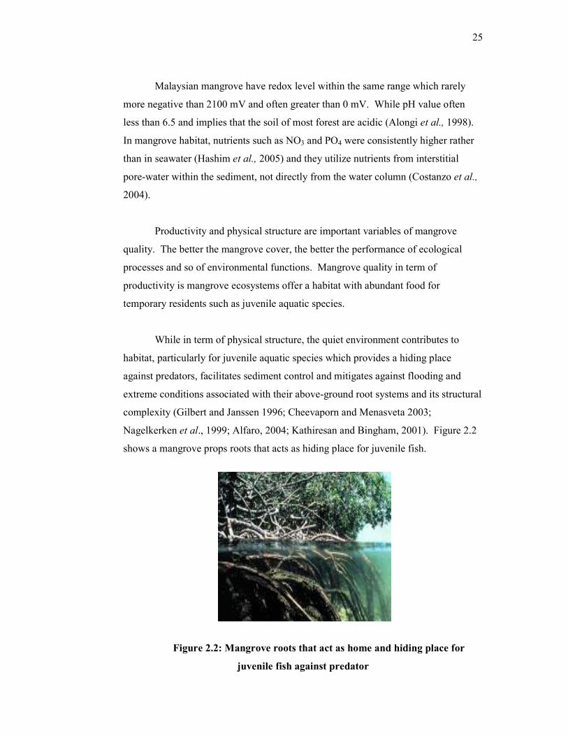
While in term of physical structure, the quiet environment contributes to

habitat, particularly for juvenile aquatic species which provides a hiding place

against predators, facilitates sediment control and mitigates against flooding and

extreme conditions associated with their above-ground root systems and its structural

complexity (Gilbert and Janssen 1996; Cheevaporn and Menasveta 2003;

Nagelkerken et al., 1999; Alfaro, 2004; Kathiresan and Bingham, 2001). Figure 2.2

shows a mangrove props roots that acts as hiding place for juvenile fish.

Figure 2.2: Mangrove roots that act as home and hiding place for

juvenile fish against predator

26

Hoai et al. (2006) were proved by measurement of wave forces and

modeling of fluid dynamics and found out that the tree vegetation may reduce wave

amplitude and energy. Analytical model shows that 30 trees from 100 m2 in a 100m

wide belt may reduce the maximum tsunami flow pressure by more than 90 percent.

Forest age will affect the organic carbon oxidation rate in mangrove

sediments. Age of mangrove can be divided into two which are mature (60 years and

more) and young (2 to 12 years) trees. Sediment becomes less inundate because it

more compacted in mature mangrove area. The abundance and diversity of infauna

also undergo declination as well as reduction of sulfate. While in younger mangrove

area, the total macrofaunal abundance is remain similar and the ability of nitrogen

and phosphorus uptake is increasing due to aerobic and suboxic role and the presence

of large numbers of surface-living (Morrisey et al., 2001; Alongi et al., 1998).

Human activities have been the primary cause of mangrove loss.

Aquaculture such as conversion to shrimp ponds and fish pond (Cheevaporn and

Menasveta 2003; Alongi et al., 1999), industrial effluent that contributes to heavy

metal contaminant in the sediment, anthropogenic influences (John and Lawson,

1990) and lubricating oils (Garrity et al., 1994; Zhang et al., 2006) would be the

main supporter to destruction of mangrove habitat.

Different geographical locations had different heavy metal concentrations,

depending on the degree of anthropogenic pollution (Tam and Wong, 2000).

Although mangrove have the ability in controlling the mobility of heavy metals

(Silva et al., 2006) with respect to the abundance type of microorganisms which

clean up the waste materials (Hashim et al., 2005), they still have tolerant limitation

and continuously decline time by time with reduction of 1 percent per year in many

developing countries (Alongi et al., 1999).

In Thailand, the existing mangrove forest has decreased more than 50% in the

past 32 years (Cheevaporn and Menasveta 2003) and based on study made by Bayen

et al. (2004), less than 0.5 percent of Singapore’s total land area are still covered by

mangroves compared to approximate 13 percent in 1820.

27

2.7 River Classification and Pollutant Status

Water Quality Index (WQI) as shown in Table 2.1 is the most important

criteria in order to determine water quality in particular water bodies and limit to

freshwater or river only. DO, BOD, COD, AN, SS and pH are common parameters

that use in determining WQI. River classification for each parameter can be

measured by using Table 2.2. The percentage of entire parameters will be evaluated

and being determine which classes are they in to.

Table 2.1: Water Quality Index (WQI) (DOE, 1986)

WQI Range Pollution Degree

< 31.0 Severely Polluted

31.0 – 51.9 Slightly Polluted

51.9 – 76.5 Moderate

76.5 – 92.7 Clean

> 92.7 Very Clean

Table 2.2: Department of Enviroments’ Water Quality Index Standard

(DOE, 1986)

Parameter Unit Class

I II III IV V

Ammoniacal

Nitrogen

mg/l < 0.1 0.1-0.3 0.3-0.9 0.9-2.7 > 2.7

BOD mg/l < 1 1-3 3-6 6-12 > 12

COD mg/l < 10 10-25 25-30 50-100 > 100

DO mg/l > 7 5-7 3-5 1-3 < 1

pH - > 7 6-7 5-6 < 5 > 5

Suspended Solids mg/l < 25 25-50 50-150 150-300 > 300

Water Quality Index > 92.75 76.5-92.7 51.9-76.5 31.0-51.9 < 31.0

Degree of river classifications that had been recommended is very clean,

clean, moderate, slightly polluted and severely polluted. Before WQI is determined,

Table 2.3 needs to be revised in order to evaluate parameters’ subindex. According

to Department of Environment (1986), WQI was summarizing from Interim National

Water Quality Standard (INWQS) for Malaysia as shown in Table 2.4.

28

Table 2.3: Parameter Subindex DOE-WQI (DOE, 1986)

Parameter Value Subindex equation (SI)

COD If X = < 20 SICOD = 99.1 – 1.33X

If X > 20 SICOD = 103 x [E]-0.0157X - 0.04X

BOD If X = <5 SIBOD = 100.4 – 4.32X

If X >5 SIBOD = 108 x [E]-0.055X – 0.1X

AN If X = < 0.3 SIAN = 100.4 – 4.32X

If 0.3 < X < 4 SIAN = 94 x [E]-0.573X – 5(X-2)

If X = > 4 SIAN = 0

SS If X = < 100 SISS = 97.5 x [E]-0.00676X + 0.7X

If 100 < X < 1000 SISS = 71 x [E]-0.0016X – 0.015X

If X= > 1000 SISS = 0

pH If X < 5.5 SIpH = 17.2 – 17.2X + 5.02X2

If 5.5 = < X < 7 SIpH = -242 + 95.5X – 6.67X2

If 7 = < X <8.75 SIpH = -181 + 82.4X – 6.05X2

If X = > 8.75 SIpH = 536 – 77X + 2.76X2

DO X = DO (mg/L) * 12.6577

If X = < 8 SIDO = 0

If 8 > X SIDO = -0.395 + 0.030X2 – 0.00019X3

WQI = (0.22 * SIDO) + (0.19 * SIBOD) + (0.16 * SICOD) +

(0.15 * SIAN) +(0.16 * SISS) + (0.12 *SIpH) 2.2

Note: (1) X is concentration of parameter in unit mg/L, except for pH and DO

(2) x is symbol of multiply

(3) SIDO, SIBOD, SICOD, SIAN, SISS and SIpH are the Sub Index (SI) of

the respective water quality parameters which isused to calculate the Water

Quality Index (WQI).

29

Table 2.4: Interim National Water Quality Standard for Malaysia (INWQS)

with related of water quality parameter (DOE, 1986)

Parameter Units Class

I IIA IIB III IV V

Ammoniacal

Nitrogen

mg/l 0.1 0.3 0.3 0.9 2.7 > 2.7

BOD mg/l 1 3 3 6 12 > 12

COD mg/l 10 25 25 50 100 > 100

DO mg/l 7 5-7 5-7 3-5 < 3 < 1

pH 6.5-8.5 6-9 6-9 5-9 5-9 -

Color TCU 15 150 150 - - -

Conductivity µmhos/cm 1000 1000 - - 6000 -

Floating N N N - - -

Odour N N N - - -

Salinity ppt 0.5 1 - - 2 -

Taste N N 50 - - -

Total

Dissolved

Solids

mg/l 500 1000 - - 4000 -

Total

Suspended

Solids

mg/l 25 50 50 150 300 > 300

Temperature ˚C - Normal±2 - Normal±2 - -

Turbidity NTU 5 50 50 - - -

E. Coli. Coloni/100ml 10 100 400 5000

(2000)ε

5000

(2000)ε

-

Total Coliform Coloni/100ml 100 5000 5000 50000 50000 > 50000

Class I represents water body of excellent quality. Standards are set for the

conservation of natural environment in its undisturbed state. Water bodies such as

those in the national park areas, fountainheads, and in high land and undisturbed

areas come under this category where strictly no discharge of any kind is permitted.

Water bodies in this category meet the most stringent requirements for human health

and aquatic life protection.

Class II A represents water bodies of good quality. Most existing raw water

supply sources come under this category. In practice, no body contact activity is

30

allowed in this water for prevention of probable human pathogens. There is a need to

introduce another class for water bodies not used for water supply but of similar

quality which may be referred to as Class IIB. The determination of Class IIB

standard is based on criteria for recreational use and protection of sensitive aquatic

species.

Class III is defined with the primary objective of protecting common and

moderately tolerant aquatic species of economic value. Water under this

classification may be used for water supply with extensive/advance treatment. This

class of water is also defined to suit livestock drinking needs.

Class IV defines water quality required for major agricultural irrigation

activities which may not cover minor applications to sensitive crops and finally

Class V represents other waters which do not meet any of the above uses.

2.8 River Classification Based on Biological Indicator

River classification based on biological assessment can be carried out

towards the rivers’ ecology criterion. The assessment of biological variety in term of

river management is mostly use Shannon-Weiner Diversity Index (H’) that measures

both richness and evenness of biodiversity (USEPA, 1980). According to Nor

Azman Kasan (2006), there is significant correlation between water quality and algae

population by compared via WQI and Shannon-Weiner Diversity Index (H’). The

equation for the index is;

ng Shannon-Weiner Diversity Index (H’) = - ∑ Pi ln Pi (2.3)

i = 1

With ng represent number of genera, Pi is ratio to each genara and ln is log 10.

According to Malaysian Water Quality Classification, river’s class can be determined

into five categories; Class I, Class II, Class III, Class IV and Class V based on H’

31

value that had been evaluated (UM-DOE, 1986, Malaysia, 1990-Phase II) as shown

in Table 2.5.

Table 2.5: Water Quality Determination based on Shannon-Weiner Diversity

Index (UM-DOE, 1986)

Shannon-Weiner Diversity

Index, H’

Classification Water Quality

> 3.73 I Very Clean

2.80-3.73 II Clean

1.86-2.80 III Moderate Pollution

0.93-1.86 IV Slightly Pollution

0.00-0.93 V Severely Pollution

CHAPTER III

METHODOLOGY

3.1 Introduction

This chapter explains on the few phases used from the beginning to the final

stage in order to achieve the objectives of this study. Before fieldwork is carried out,

there are a few scopes and methodology inflows that need to follow to ensure the

information is well gain in order to make study easier in term of data assemblages

and editing.

3.2 Literature Review

Information related to Sungai Batu Pahat is gathered from variety sources

including maps, internet, books, journal, news articles, magazine, and thesis book

from previous student. This source is catered at Perpustakaan Sultanah Zanariah

(PSZ), Universiti Teknologi Malaysia (UTM) and Pusat Sumber Fakulti

Kejuruteraan Awam (FKA), UTM. Beside, interviewing with expert, local

communities, fisherman and related authorities such as Department of Forestry, and

Deparment of Environment (DOE) also involved.

33

3.3 Determine the Parameter Involved

Parameters that involved in this study are divided into two which are Water

Quality Index (WQI) and biodiversity parameters. WQI consist of commonly six

parameter which are Dissolved Oxygen (DO), Biochemical Oxygen Demand (BOD),

Chemical Oxygen Demand (COD), Suspended Solids (SS), acidic and alkalinity

(pH) and Nitrogen-Ammonia (NH3-N). While biodiversity comprise of fishes,

zooplankton, phytoplankton, benthos and riverbank vegetation.

3.4 Sampling Method

The sampling station for both parameters was determined by using

topography map with serial number DNMM 6102 Edition 1-PPNM Sheet 168a & c

and was categorized into three portions of stream which is upstream, middle stream

and downstream as shown in Figure 3.2. At the middle stream, 3 sampling point was

choosen, while at the upstream and downstream, 2 sampling point for each. GPS

(Geographical Positioning System) Etrex Summit model as shown in Figure 3.1 was

used to determine each coordinate of water quality stations.

Figure 3.1: Geographical Positioning System was used to determine

coordinate and distance

34

Water quality parameter was taken three times within August and September

2006 which is three times during high tide and three times during low tide. While for

biodiversity parameter was taken twice on August and September 2006 at five station

as shown in Figure 3.2 which is two times during high tide and two times during low

tide but for riverbank vegetation, only one shot coordinate sampling because no

alteration was observe within sampling events. Figure 3.3, Figure 3.4 and Figure 3.5

shows upstream, middlestream and downstream of sampling station respectively.

Figure 3.6 shows riverbank vegetation during high tide while Figure 3.7 shows low

tide’s scene of riverbank vegetation.

Figure 3.2: Portions of Water Quality Sampling Station at Sungai Batu Pahat

UPSTREAM

MIDDLE STREAM

DOWNSTREAM

35

Figure 3.3: Upstream of Sungai Batu Pahat. Patches of Nypa habitat are

abundance at the upstream because of low salinity water compared to seaward.

Water seems to be cleaner from turbidity

Figure 3.4: A lot of shipping activity occurred at the middle stream of the

estuary, resulting disturbance of biodiversity and riverbank vegetation as well

as water quality depletion

36

Figure 3.5: Downstream of Sungai Batu Pahat is adjacent to coastal water that

have wide opening. At downstream, the land are fully covered by riverbank

vegetation especially mangrove in order to protect against tsunami

Figure 3.6: Sungai Batu Pahat during high tide. Fresh water from the river is

mixing with coastal water and abundance of fish will take this opportunity to

breed at vegetations’ roots

37

Figure 3.7: During low tide, the roots of vegetation were clearly seen and this is

the time for adult fish go to open sea because, water from estuary was flowing

seaward during this period

3.4.1 Water Quality Sampling

‘In-situ’ parameter such as pH and DO was determined by using Multi-

Parameter Analyzer-Consort C535 (Figure 3.8) and 55-YSI Dissolved Oxygen Meter

(Figure 3.9) respectively. While the rest of parameter will be analysis at laboratory

by taken water sample into 2 liter polyethylene bottle which was clean according to

Standard Method APHA 4500-P. The water sample then being preserved by put a

few drops of nitrite acid (H-NH3) and stored at 4°C cold room as soon as BOD

analysis carried out in order to minimize biological activities in the water.

Figure 3.8: Multi-Parameter Analyzer-Consort C535 that had been used

to determine pH level on surface water of Sungai Batu Pahat

38

Figure 3.9: 55-YSI Dissolved Oxygen Meter was used in order to get dissolved

oxygen concentration in unit mg/L on surface water

3.4.2 Fisheries Sampling

Fishes was caught using cast net (Figure 3.10) and trammel net (Figure 3.11)

within August and September, 2006 which is 2 times during neap high tide and 2

times during low tide to high tide. Cast net was used with opening diameter

approximately 2.43 m (8 feet) and mesh size is 2.54 cm (1 inch). Besides, 2 trammel

net was used with 3 layers and each layer has of length 100m. Each trammel net has

2 outside layer with mesh size 10.16 cm (4 inch) and 1 inside layer with mesh size

3.81 cm (1.5 inch). Sampling was carried out 5 times using trammel net and 30

times using cast net and let it on water column for about 30 minutes before identified

the fish species, measure fish length and weight, and evaluate total fish that had been

caught.

Figure 3.10: Cast net had been used thirty (30) times for fish sampling

39

Figure 3.11: Trammel net was used for five (5) times at certain part of the river

where drift net using is allowed

3.4.3 Phytoplankton

Phytoplankton had been sampled at five stations as shown in Figure 3.1.

Water samples were sampled at 0.5m depth from the water surface by using a Van

Dorn Sampler (4.2L) as shown in Figure 3.12. For each replicate, water was

sampled three times and sieved through the 10µm mesh size to concentrate the

phytoplankton samples. The remains of plankton net cod-end were then preserved

with 10% of buffered formaldehyde for laboratory analysis.

Figure 3.12: Water sampling using Van Dorn Sampler in order to identify

phytoplankton assemblages

40

At the laboratory, phytoplankton samples were pipette onto the Sedgewick

Rafter cell and examined under a compound microscope. The phytoplankton was

identified to genus level where possible and photo of dominated phytoplankton

species within Sungai Batu Pahat can be seen at Appendix E.

3.4.4 Zooplankton

Plankton net with 30cm mouth diameter and 147µm mesh and a calibrated

flowmeter was used to sample zooplankton at 0.5m depth (Holguin et al., 2005;

Prepas and Charette, 2003; Lampman and Makarewicz ,1999; Johannsson et al.,

1986) from the water surface as shown in Figure 3.13. The samples were collected

into the plankton bottle and preserved with 10% of buffered formaldehyde for

laboratory analysis.

Figure 3.13: Zooplankton had been caught using plankton net at 0.5m depth

from the water surface

At the laboratory, zooplankton samples were sieved through 53µm Endecott

sieve using running tap water. Particles with sizes smaller than 53µm had been

removed. The zooplankton fraction was transferred onto pre-weighed steel gauze and

excess moisture was absorbed by blotting towel.

41

According to Rougier et al. (2004), 150 mm mesh size is using for

mesozooplankton capture and the other with a 40 mm mesh size is for

microzooplankton capture including rotifers. Wet weight was measured to 2 decimal

points. All samples were then kept separately in storage bottle with 85% alcohol for

subsequent examination.

For enumeration and identification purposes zooplankton samples was

subsampled by using a Stempel pipette and transfer onto a Sedgewick-Rafter cell.

Zooplankton density was determined by counting the zooplankton individuals in the

cell. Sample was split into two or more times if sample was large by using a Folsom

plankton splitter.

3.4.5 Macrobenthos

Macrobenthos samples were collected from upstream of the study area to

adjacent coastal water as shown in Figure 3.2. Figure 3.14 shows an Ekman grab

sampler that used to collect sediment. The sediment was sieved through 500µm

Endecott sieve on board. The entire materials on sieve were collected into a plastic

bag and preserved with 10% of buffered formaldehyde for laboratory analysis.

Figure 3.14: Ekman grab sampler that used to identify benthic animals with

500µµµµm Endecott sieve on board

42

At the laboratory, the materials in the plastic bag were poured onto an enamel

tray. The benthic animals were sorted and identified using a binocular microscope.

Plant debris and shell materials were also recorded.

3.4.6 Riverbank Vegetation Analysis

Coordinate along the river via boat and road was taken approximate every 10

meter in order to measure the riverbank area that still covered by vegetation

including mangrove, nypa and secondary shrubs using GPS. With coordinate data

collection, area of vegetation then is calculated using Google Earth Pro. However,

the results only show an approximate value, not the actual one which is align to this

study objective which to what extent the biodiversity may survive with the presence

of riverbank vegetation beside rely on water quality alone.

Type of existing vegetation along the river was given by Department of

Forestry Johor Tengah. Interview session with forestry personel, was carried out to

gain related information.

3.5 Chemical Analysis

There are important equipments that being used during chemical analysis

including beaker 2000 mL, measurement cylinder 10 mL, 25 mL, 100 mL, and 1000

mL as well as 10 mL pipette which was cleaned comply to Standard Methods APHA

4500-P. The whole equipments and tools was provided by Environmental

Engineering Laboratory, Faculty of Civil Engineering, Universiti Teknologi

Malaysia (UTM).

43

3.5.1 Concentration Measurement Of Biochemical Oxygen Demand (BOD5)

To determine BOD5, Standard Method APHA 5210-B is using to evaluate

dissolved oxygen that contain in water sample.

3.5.2 Concentration Measurement Of Chemical Oxygen Demand (COD)

COD value was evaluated by HACH Model DR/4000 Spectrometer which

comply to Standard Methods APHA 5220-C where water sample being reflux using

COD Reactor Model HACH.

3.5.3 Concentration Measurement Of Nitrogen-Ammonia ((NH3-N)

Standard Method APHA 4500-NH3-BC was used to evaluate Nitrogen-

Ammonia’s (NH3-N) value through HACH model DR/4000 Spectrometer which

created by HACH Company, Loveland, Colorado, USA.

3.5.4 Measurement of Suspended Solids (SS)

For Suspended Solids measurement, all procedures was complied to Standard

Methods APHA 2540-D

3.6 Data Analysis

For physicochemical analysis, Water Quality Index (WQI) and Interim Water

Quality Standard (INWQS) provided by Department of Environment (DOE) were

44

referred to identify the status and classification of Sungai Batu Pahat. The result will

be represented as graph form, utilize Microsoft Excel and CurveExpert software and

the profile of each parameter was determined. Biodiversity data were compared to

previous related studies in order to identify the characteristic and diet of species in

general. The relationship between physicochemical parameter and biodiversity

parameter was examined such as between WQI and biodiversity population, WQI

and vegetation habitat, as well as between biodiversity population and vegetation

habitat.

CHAPTER IV

RESULT AND ANALYSIS

4.1 Introduction

It is well known those mangroves are the salt tolerant forest ecosystems

found in tropical and sub-tropical intertidal regions of the world. They consist of

swamps, forest-land and water-spread areas. These forest ecosystems support marine

fisheries and protect the coastal zone, thus helping the coastal environment and

economy. These ecosystems are biologically productive, but ecologically sensitive.

A lot of factors that contribute to water quality degradation of Sungai Batu Pahat

such as population growth and accompanying land use changes.

Sungai Batu Pahat is situated at Bandar Penggaram and most of the riverbank

had altered into resident area, urban area and shipping activities. It is important to

rehabilitate the water quality within Sungai Batu Pahat because it supports fisheries

as protein diet and livelihood for community nearby as well as for biological

community such as otter and water birds. As mention before in literature review,

Sungai Batu Pahat received a visit from threatened bird’s species-one species of

stork, the Lesser Adjutant (Leptoptilos javanicus). Thus, it is important to identify

the water quality status of the river to ensure fish survival as well as the quality of

food for them (planktonic life and benthic macroinvertebrates). Riverbank

vegetation especially mangrove plays a main role in order to maintain the quality

food for fish survival. Therefore, the existing riverbank vegetation should be

protected from further degradation.

46

4.2 Land Use Analysis

Batu Pahat can be characterized as agricultural land which is covers 83% of

the total area of Batu Pahat as shown in Table 4.1 followed by forestry with 5.62% of

Batu Pahat. Residential area only covers 3.43% with 6,444 ha and other related land

uses are commercial area, institutional and facilities, open space and recreational

area, and industrial area. However, water bodies at Batu Pahat merely 1.54% or

2,887 ha from total area of Batu Pahat and it is not impossible if quality of water

bodies at Batu Pahat were interrupted by land use activities especially from

agriculture run off.

Table 4.1: Distribution of exiting land use in Batu Pahat (MPBP, 2002)

The land use activities around Batu Pahat seem to be a major contributor in

determining the water quality of Sungai Batu Pahat. According to Majlis

Perbandaran Batu Pahat (MPBP, 2002), there is 525 gazetted villages and village-

cluster at Batu Pahat district where smaller villages were annexed to their bigger

immediate neighbors for the purpose of administration. The land use in Batu Pahat

consists of 2 main areas; town centre and the rural areas. In town centre, most of the

land uses are industrial, commercial and residential area while agricultural activities

and small village are located at the rural area.

Land Use Hectare Percent (%)

Agricultural Area 156,070 83.15

Forestry 10,550 5.62

Water body 2,887 1.54

Residential Area 6,444 3.43

Business Area 330 0.18

Industrial Area 918 0.49

Institutional and Facilities 1,387 0.74

Open Space and Recreational

1,266 0.67

Reserve land 4,126 2.20

Total 187,702 100

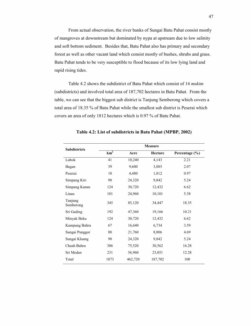
47

From actual observation, the river banks of Sungai Batu Pahat consist mostly

of mangroves at downstream but dominated by nypa at upstream due to low salinity

and soft bottom sediment. Besides that, Batu Pahat also has primary and secondary

forest as well as other vacant land which consist mostly of bushes, shrubs and grass.

Batu Pahat tends to be very susceptible to flood because of its low lying land and

rapid rising tides.

Table 4.2 shows the subdistrict of Batu Pahat which consist of 14 mukim

(subdistricts) and involved total area of 187,702 hectares in Batu Pahat. From the

table, we can see that the biggest sub district is Tanjung Semberong which covers a

total area of 18.35 % of Batu Pahat while the smallest sub district is Peserai which

covers an area of only 1812 hectares which is 0.97 % of Batu Pahat.

Table 4.2: List of subdistricts in Batu Pahat (MPBP, 2002)

Measure Subdistricts

km2 Acre Hectare Percentage (%)

Lubok 41 10,240 4,143 2.21

Bagan 39 9,600 3,885 2.07

Peserai 18 4,480 1,812 0.97

Simpang Kiri 98 24,320 9,842 5.24

Simpang Kanan 124 30,720 12,432 6.62

Linau 101 24,960 10,101 5.38

Tanjung Semberong

345 85,120 34,447 18.35

Sri Gading 192 47,360 19,166 10.21

Minyak Beku 124 30,720 12,432 6.62

Kampung Bahru 67 16,640 6,734 3.59

Sungai Punggor 88 21,760 8,806 4.69

Sungai Kluang 98 24,320 9,842 5.24

Chaah Bahru 306 75,520 30,562 16.28

Sri Medan 231 56,960 23,051 12.28

Total 1873 462,720 187,702 100

48

4.2.1 Residential

It is well known that over population is the major contributor to degradation

of water quality (Franca et al., 2005; Smith, 2004; Butcher et al., 2003; Lin et al.,

2006). Based on survey made by Majlis Perbandaran Batu Pahat (MPBP, 2002),

nowadays, it is estimated that approximately 400, 000 residents are living in Batu

Pahat with Simpang Kanan being the most dense subdistrict in Batu Pahat with 139,

640 people while the least populated is Bagan with only 4, 692 people. The town

itself has 140, 000 local resident and most houses in this town are single or double

storey terrace houses as well as wooden houses.

Majority of people living along Sungai Batu Pahat dump solid waste as well

as sewage directly into water bodies with respect to lack or no proper sewage

treatment system and solid waste collection system. Due to uncontrolled discharge

of organic matter in estuaries regions, the water bodies will lead to anoxic condition

(Desa et al., 2005).

Figure 4.1 shows some squatters which are located by the river. They also

create their own dumping ground nearby the river that may causes leachate leaching

to estuaries during rainy days resulting depletion of water quality. Figure 4.2 shows

dumping ground made by local communities

Figure 4.1: Squatter area located by the river with improper sewage treatment

and solid waste collection system

49

Figure 4.2: Dumping area that made by local resident and resulting poor view

and bad odour

Beside as ‘dumping area’, Sungai Batu Pahat also acts as route for them to

get to town that located just the other side of the river. It is easier to cross over the

river by boat rather than use road which take a long period because of traffic jam.

Most of the people here have lived here for a long time and likes it here because it is

a complete town with all the basic facilities and it is also very convenient to get

around town.

4.2.2 Agricultural and Farming

Batu Pahat is mostly covered by agriculture activities and also has a wide

area of primary forest which is known as Hutan Simpan Gunung Banang. Riverbank

vegetation that exists along Sungai Batu Pahat will be discussing detail in other sub

topic. Palm oil plantation, rubber plantation and coconut plantation are identified as

the main agricultural activities in Batu Pahat. Discussing about agriculture, we could

never escape from the chemical substance used for plantation growth such as

insecticide, pesticides and fertilizers which might contribute to high amounts of

phosphate in the estuaries.

50

Non point sources of nutrients (from agricultural activities, fossil-fuel

combustion, and animal feeding operations) are often of greater concern than point

sources because they are larger and more difficult to control (Thomas, 2004). The

chemical substance will released abundance into estuaries especially during rainy

days which carried by the storm water runoff as well as animal manure from farming

activities that also flow with the runoff. All these activities will contribute to high

content of ammonia nitrogen in the river.

4.2.3 Commercial

Commercial area is located at the centre city of Batu Pahat and would be the

contributor to river pollution. Human activities such as restaurants, car and motor

services, wet market, hospital and clinics may release a lot of pollutant whether like

it or not. Market and restaurant contribute much organic substance into the water

bodies.

Figure 4.3: Trade activities along Sungai Batu Pahat that trades goods and

groceries such as logs and timbers

Figure 4.3 shows a barter-trade jetty handling import and export of goods

locally and Indonesia that located along Sungai Batu Pahat. As we can seen from

this figure, the port is unsystematically management and messy as well as busier

since the decreasing of such trades in Singapore ports (Low, 2007). Beside oil

51

spillage from ships during loading and unloading goods, workers also tend to dump

waste into the estuaries and increased the chances for water quality to be

deteriorated.

4.2.4 Industrial

Industrial activities are considered as point sources that released less essential

nutrient than non point sources (Sarkar et al., 2005; Thomas, 2004; Alongi et al.,

1998; Simpson and Pedini, 1985). In Batu Pahat, the main industrial activity is

manufacturing of textile with 40% of total textile industry in Malaysia especially the

wet processing plants. This could due to its strategic location for industrial growth

with easy access. Malaysian Knitting Manufacturers Association (MKMA, 1996)

estimated that about 15 out of 40 plants are located in Batu Pahat and most of them

are found at the upstream of Sungai Batu Pahat.

Textile manufacturing is the major income for resident living here, but

improper management of wastewater plant there will lead to heavy metal

contaminant discharged to Sungai Batu Pahat especially the dye used which may

leave a permanent stain to the river and also resulting high turbidity, thus light cannot

penetrate deep beneath the surface.

Based on study made by Rojali Othman (1995), Batu Pahat has rubber

processing factory which process natural latex and is owned by Berjaya Group.

Unfortunately, most of the factories have improper effluent treatment system and this

will make water quality become worst and only tolerant species of fish may survive

in Sungai Batu Pahat.

Wood, brick, steel and other building materials manufacturing are identified

at Batu Pahat region together with sago, rubber, palm oil processing, furniture, and

food production. These activities will create abundance of organic substance which

are not biodegradable as well as chemical and toxic waste that finally discharged into

water column.

52

Another industrial activity that observed at Batu Pahat is quarries with about

7 quarries there such as Batu Pahat Quarry, Lian Huat Granite Quarry, Asia Quarry,

Medan Quarry and Hanson Quarry. Quarries also pose serious threat to water quality

due to its high release of suspended solids and interrupt sediment communities by

fallen of gravel onto estuaries from barges carrying gravel. Figure 4.4 shows one of

the quarries by the river that potentially become the major contributor to degradation

of water quality at Sungai Batu Pahat.

Figure 4.4: Busy quarry activities during day time along Jalan Minyak Beku

closed to Sungai Batu Pahat

4.3 Water Quality Analysis

In Malaysia, there are six main water quality parameter that strongly

recommended by Department of Environment (DOE) in order to classifying the

status of particular water bodies. The parameters are dissolved oxygen (DO),

biochemical oxygen demand (BOD), chemical oxygen demand (COD), ammoniacal

nitrogen (NH3-N), suspended solids (SS) and finally, alkalinity and acidity (pH). In

this study, the water quality was analyzed between low tide and high tide along 10.43

km length of the river.

53

Water quality were sampling three times for high tide and three times during

low tide within August 2006 and September 2006. The result of each parameter is an

average value of sampling frequency. Table 4.3 shows each parameter result during

high tide while Table 4.4 shows low tide’s water quality parameter result. From both

of the table below, COD during low tide was higher than high tide due to abundance

of inorganic effluent that discharged from land use activities while other parameters

shows almost equal value.

Table 4.3: Water quality parameter result during high tide

Table 4.4: Water quality parameter result during low tide

Sampling Distance from Water Quality Index Parameter (mg/L), except for pH

Station Station 1 DO BOD COD SS AN pH

1 0 3 3.82 60 6.7 1.03 3.13

2 2.5 3.04 8.61 61 10.1 1.18 3.66

3 3.21 3.86 19.88 77 1.5 1.07 4.67

4 4.42 4.2 20.58 71 7.5 1.17 5.14

5 6.26 3.3 19.88 74 18.3 1.09 3.54

6 7.78 3.89 20.3 74 24.9 0.875 4.48

7 10.43 6.61 18.06 230 165.5 0.328 6.21

Sampling Distance from Water Quality Index Parameter (mg/L), except for pH

Station Station 1 DO BOD COD SS AN pH

1 0 3.73 4.31 79 42.4 1.01 3.42

2 2.5 1.07 9.31 90 8.7 1.30 3.66

3 3.21 1.37 13.02 34 2.4 1.08 3.64

4 4.42 2.13 21.14 277 8.5 1.08 3.86

5 6.26 2.68 15.96 207 27.9 0.75 4.12

6 7.78 1.98 14.56 120 41.2 0.798 5.17

7 10.43 5.89 19.88 720 103.1 0.555 6.38

54

After the concentration of each parameter was catered, Table 2.3 as shown in

chapter II previously was used in determining the subindex of each parameter and

finally the water quality index and its class were determined by using Table 2.1 and

Table 2.2. Table 4.5 shows the result of subindex during high tide while during low

tide as shown in Table 4.6. From the both of the table, it is obviously seen that,

water quality during high tide much better rather than during low tide as consequence

of mixing water that create high turbulence and gradient.

Table 4.5: Water quality subindex parameters result during high tide

Sampling Water Quality Subindex WQI Class

Station SIDO SIBOD SICOD SISS SIAN SIpH

1 32 84 38 98 57 13 55 III

2 33 66 37 98 52 21 52 III

3 49 34 28 98 56 46 51 IV

4 56 33 31 98 52 73 56 III

5 38 34 29 99 55 19 46 IV

6 50 33 29 100 63 41 52 III

7 98 38 -6 52 86 94 60 III

Table 4.6: Water quality subindex parameters result during low tide

Sampling Water Quality Subindex WQI Class

Station SIDO SIBOD SICOD SISS SIAN SIpH

1 46 82 27 103 58 17 57 III

2 5 64 21 98 48 21 42 IV

3 8 51 59 98 55 21 47 IV

4 18 32 -10 98 55 26 35 IV

5 27 43 -4 100 67 32 43 IV

6 15 47 11 103 66 73 49 IV

7 84 34 -29 59 76 96 53 III

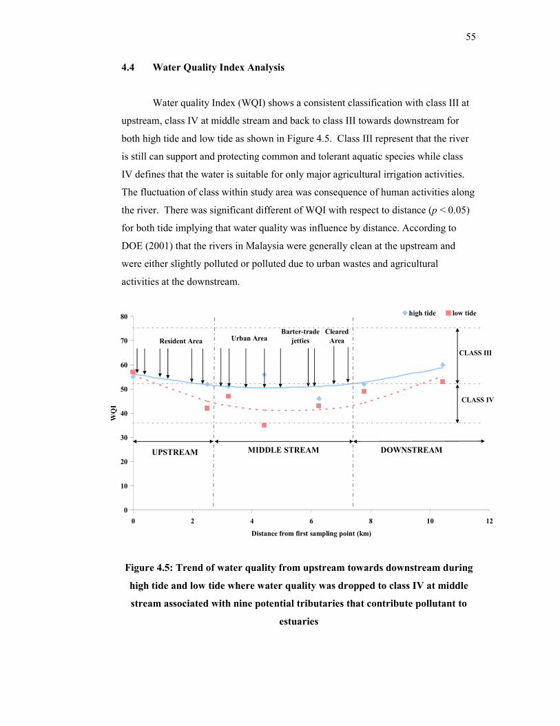
55

4.4 Water Quality Index Analysis

Water quality Index (WQI) shows a consistent classification with class III at

upstream, class IV at middle stream and back to class III towards downstream for

both high tide and low tide as shown in Figure 4.5. Class III represent that the river

is still can support and protecting common and tolerant aquatic species while class

IV defines that the water is suitable for only major agricultural irrigation activities.

The fluctuation of class within study area was consequence of human activities along

the river. There was significant different of WQI with respect to distance (p < 0.05)

for both tide implying that water quality was influence by distance. According to

DOE (2001) that the rivers in Malaysia were generally clean at the upstream and

were either slightly polluted or polluted due to urban wastes and agricultural

activities at the downstream.

Figure 4.5: Trend of water quality from upstream towards downstream during

high tide and low tide where water quality was dropped to class IV at middle

stream associated with nine potential tributaries that contribute pollutant to

estuaries

0

10

20

30

40

50

60

70

80

0 2 4 6 8 10 12

Distance from first sampling point (km)

WQI

high tide low tide

UPSTREAM MIDDLE STREAM DOWNSTREAM

CLASS IV

CLASS III

Resident Area Urban AreaBarter-trade

jetties

Cleared

Area

56

However, the situation was differing for Sungai Batu Pahat. This was caused

by human refuse which common at almost all mangrove estuaries of similar size and

type in Malaysia. High suspended loads and high nutrient concentration was found

at Southeast Asia in consequence of high rates of river runoff, shoreline erosion,

resuspension, heavy boat traffic, agricultural and forest runoff, and dumping waste

(Alongi et al., 2003). The source of water quality deteriorating towards middle

stream is because of discharging from heavy boat traffic, quarry activities, and

settlement activities at adjacent river.

The major reason of depleting water quality at middle stream is it located at

urban area (non-industrial area) that discharges effluent via drainage and tributaries.

Anthropogenic effects are stronger at the estuaries since water circulation is much

more limited than the coastal ecosystem (Ahsen et al., 2006). From observation,

there were nine potential tributaries that contribute to decreasing of water quality at

middle stream (average value of WQI is 51.0 and 41.7 for high tide and low tide,

respectively). Clearance area for proposed development also the main contributors

which release nutrient and heavy metals that supposed to uptake by mangrove into

estuaries. Mangrove is recognize as controller of heavy metal mobility because of its

varies clean up microorganisms (Silva et al., 2006; Hashim et al., 2005). It is well

known that, for non-industrial area, the sources that likely to have is traffic emission

and road runoff, city wastewater and biosolids used as fertilizer (Zhang et al., 2006).

However, the upstream of study area shows slightly polluted with average

value of water quality index (WQI) is 53.2 and 49.5 for high tide and low tide,

respectively. It was due to agriculture runoff and road runoff. The upstream of the

study area is not located exactly at the upstream of the estuaries but located at the

upstream of new proposed development area that situated downstream of Sungai

Batu Pahat. Thus, the water quality still hampered by local communities’ activities

such as agricultural which mostly found at the upstream of Sungai batu Pahat.

As well as the downstream of study area, the WQI shows class III which is

slightly polluted. Downstream of Sungai Batu Pahat is at adjacent coastal water that

has wide open to Straits of Melaka. According to Azrina et al. (2006), downstream

being usually characterized by greater width, lower flow rate, and softer bottom.

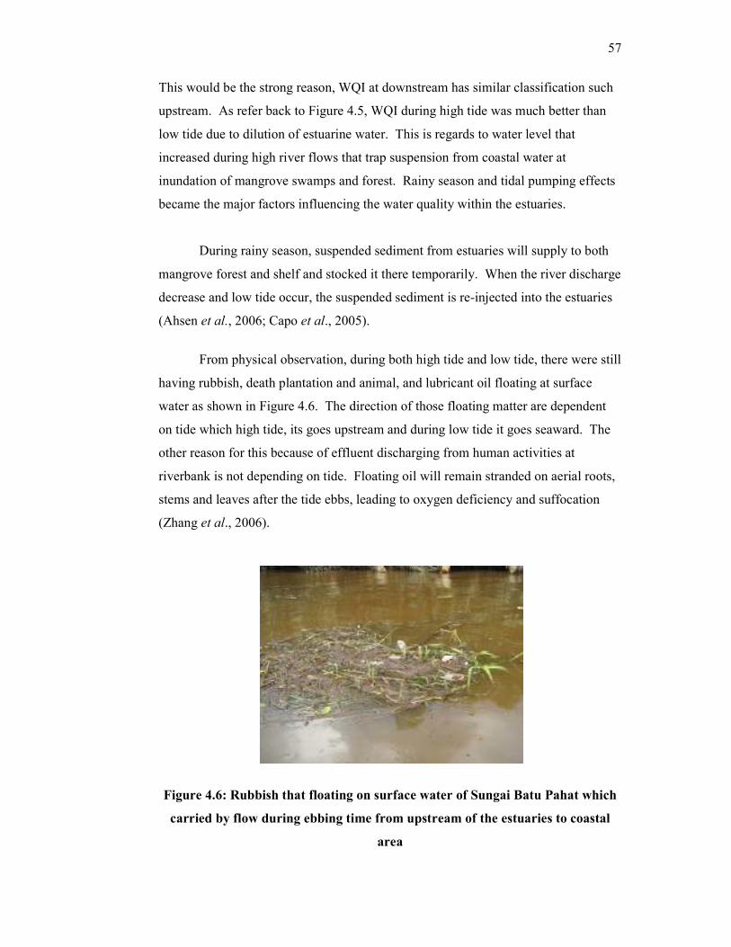
57

This would be the strong reason, WQI at downstream has similar classification such

upstream. As refer back to Figure 4.5, WQI during high tide was much better than

low tide due to dilution of estuarine water. This is regards to water level that

increased during high river flows that trap suspension from coastal water at

inundation of mangrove swamps and forest. Rainy season and tidal pumping effects

became the major factors influencing the water quality within the estuaries.

During rainy season, suspended sediment from estuaries will supply to both

mangrove forest and shelf and stocked it there temporarily. When the river discharge

decrease and low tide occur, the suspended sediment is re-injected into the estuaries

(Ahsen et al., 2006; Capo et al., 2005).

From physical observation, during both high tide and low tide, there were still

having rubbish, death plantation and animal, and lubricant oil floating at surface

water as shown in Figure 4.6. The direction of those floating matter are dependent

on tide which high tide, its goes upstream and during low tide it goes seaward. The

other reason for this because of effluent discharging from human activities at

riverbank is not depending on tide. Floating oil will remain stranded on aerial roots,

stems and leaves after the tide ebbs, leading to oxygen deficiency and suffocation

(Zhang et al., 2006).

Figure 4.6: Rubbish that floating on surface water of Sungai Batu Pahat which

carried by flow during ebbing time from upstream of the estuaries to coastal

area

58

4.5 Water Quality Parameter Analysis

Depending on water quality index (WQI) alone does not explain the real and

actual contributor to deteriorating of water quality at Sungai Batu Pahat. Because of

that, analysis of each parameter was insisted to carry out in order to identify either

organic matter or inorganic matters that contribute the most of the WQI dropping to

class IV at middle stream.

4.5.1 Dissolved Oxygen

Generally, dissolved oxygen (DO) was increasing towards downstream for

both tides as shown in Figure 4.7. At upstream, DO concentration during low tide

was higher 19.57% as compared during high tide. It is due to freshwater discharge

from Sungai Simpang Kiri and Sungai Simpang Kanan into estuaries that contain

much Dissolved Oxygen.

Figure 4.7: The fluctuation of dissolved oxygen concentration during high tide

and low tide with respect to distance which is increased towards downstream

0

1

2

3

4

5

6

7

0 2 4 6 8 10 12


DO (mg/L)

high tide

low tide

59

At distance of 2.5 km from station 1, DO concentration was dropped about

71.32% during low tide but increased during high tide with 1.33%. The DO

concentration was continuously increased at length of 3.21 km and 4.42 km with

3.86 mg/L and 4.2 mg/L respectively during high tide but dropped to 3.3 mg/L at

distance of 6.62 km because of effluent releasing from barter-trade jetties, quarry and

cleared mangrove area such as solid waste, lubricant oils, granite and sediments.

As well as during low tide, DO concentration was increased until reach to

6.26 km from station 1 with 1.37 mg/L (3.21 km), 2.13 mg/L (4.42 km) and 2.68

mg/L at 6.26 km of distance. After pass by 6.26 km from station 1, the concentration

of dissolved oxygen was rapidly increased with 3.89 mg/L (7.78 km) to 6.61 mg/L

(10.43 km) during high tide which is 41.14 % increasing while 1.98 mg/L (7.78 km)

to 5.89 mg/L (10.43 km) during low tide with 66.38 % increasing.

The rapid increasing of DO level towards downstream probably because of

abundance of DO at coastal water which have wide-range of area with cooler water

and high velocity (Thampanya et al., 2005). According to Smith (2004), Corbitt

(1999) and Nor Azman Kassan (2006), cooler water has a higher saturation point for

DO than warmer water and water that is flowing at higher velocities can hold more

DO than slower water.

Dissolve oxygen at Sungai Batu Pahat can be described as low DO as

consequence of nutrient over-enrichment and become one of the most prominent

stressor of estuarine and coastal aquatic biota. Low or no DO is well recognized as

hypoxia or anoxia circumstance was closely associated with low shell fish production

and massive fish kills in many systems (Weisse and Stadler, 2006; Donald et al.,

2002).

4.5.2 Biochemical Oxygen Demand

Biochemical oxygen demand (BOD) is one of essential parameter in order to

determine organic pollutant level as consequence of domestic wastes, agricultural

60

waste and anthropogenic inputs (Hoai et al., 2006; Hernandez-Romero et al., 2004).

Figure 4.8 shows the profile of BOD concentration towards the adjacent coastal

water. BOD concentration during high tide was increasing from 3.82 mg/L at station

1 to 8.61 mg/L at distance of 2.5 km. At distance of 3.21 km and onwards till 10.43

km, BOD concentration was consistent with 19.88 mg/L, 20.58 mg/L, 19.88 mg/L,

20.3 mg/L and 18.06 mg/L respectively.

Figure 4.8: For both tides, BOD concentration was increased from upstream

and constant as reach at distance 3.21 km to seawards due to human activities at

middle stream and undisturbed mangrove area at downstream which is known

as abundance organic matter contributor to water bodies

While during low tide, BOD concentration also increase at upstream which is

from 4.31 mg/L to 9.31 mg/L. The concentration of BOD also seem to be constant at

distance 3.21 km till 10.43 km with 13.02 mg/L, 21.14 mg/L, 15.96 mg/L, 14.56

mg/L and 19.88 mg/L respectively. From the value obtained here, it can clearly see

that, during low tide and high tide, organic loading is almost equal. The reason of

consistency of BOD concentration probably due to fluctuation of DO concentrations.

0

5

10

15

20

25

30

0 2 4 6 8 10 12


BOD (mg/L)

high tide

low tide

61

From ANOVA analysis, there is significant different (p < 0.05) between DO and

BOD with 95% confident levels. Meaning that, lower BOD concentration is directly

related to increasing of DO level and vise versa. This phenomenon is common as

identified in many previous studies (Metcalf and Eddy, 2004; Nor Azman Kasan,

2006; Peavy et al., 1986; Terbut, 1983).

At middle stream which has busy human activities, BOD was increasing (at

distance of 3.21 km to 6.26 km) because according to Lung (2001), squatters

activities that release untreated sewage and food wastes directly into water bodies

will finally increase the BOD concentration. However, towards downstream which

is at shipping activities, clear area, and onwards, BOD was consistent due to wide-

range area and organic matters were well distributed because of mixing water and

strong current by coastal water (Sholkovitz, 1985; Wang, 1978).

The other reason was probably because of less organic matter discharged at

middle stream but high non-biodegradable matter released as stated by previous

study that industrial activities discharge a lot of non-biodegradable effluent into

estuaries (Pekey, 2006; Chen et al., 2006; Zhang et al., 2006; Franca et al., 2005;

Shtiza et al., 2004; Thévenot et al., 2003; Ashkan, 2000). Even though there were

less land use activities at downstream with no potential pollutant contributor

tributaries, but the BOD concentration still higher. The organic matter may be

provided by mangrove area along the river as well as decaying of aquatic plantation

such as phytoplankton (Hoai et al., 2006; Ahsen et al., 2006; Delizo et al., 2005;

Alongi et al., 2001; Kitheka et al., 1996; Rao et al., 1982)

4.5.3 Chemical Oxygen Demand

COD refer to the quantity of oxygen required to oxidize a complete organic

substance chemically to form Carbon Dioxide (CO2) and water (H2O). The

deteriorating of water quality can be measured with high value of COD and lower

value of COD represents the other way around. Results in Figure 4.9 shows that the

average value during high tide for upstream was 60.5 mg/L, at downstream the

62

concentration increased with 74.0 mg/L and 152 mg/L towards downstream whereby

during low tide, COD value was much higher than high tide with 84.5 mg/L

(upstream), 172.7 mg/L (middle stream) and 420 mg/L (downstream). It was

obviously seen that, at middle stream, which has a lot of human activities such as

commercial area, industrial area and settlement area, the COD concentration was

increased rapidly during low tide due to non-biodegradable discharged. While the

value of COD is generally constant from upstream towards the adjacent coastal water

during high tide due of waters’ mixing between marine water and freshwater

resulting dilution.

However, at downstream, COD is increasing due to high organic and

inorganic substance that imported from Straits of Melaka water as well as from

mangrove swamps that well recognized with abundance of organic matter. In

tropical coastal-wetland in Southern Mexico, the COD value was high associated

with mangrove enriched organic matter (Sarkar et al., 2005; Hernandez-Romero et

al., 2004).

Figure 4.9: COD concentration that consistent seaward for high tide because of

dilution from coastal water. However, during low tide, COD was increased at

middle stream due to leaching of organic matter and inorganic matter from

mangrove area, urban area, as well as decaying of aquatic plants

0

100

200

300

400

500

600

700

800

0 2 4 6 8 10 12


COD (mg/L)

high tide

low tide

63

4.5.4 Ammoniacal Nitrogen

The major sources of ammoniacal nitrogen are herbicide, pesticide and

fertilizer from agricultural and farming activities, detergent from diurnal resident

activities and animal manure from pig farm. At upstream, the average value of NH3-

N was 1.11 mg/L as well as at middle stream, but at downstream the value decrease

to 0.60 mg/L during high tide. During low tide, NH3-N value was 1.16 mg/L at

upstream, drop to 0.97 mg/L at middle stream and continuous decreasing at

downstream as shown in Figure 4.10.

Figure 4.10: Ammoniacal nitrogen decreasing seawards for high tide and low

tide due to increasing of dissolved oxygen concentration

The decreasing concentration of NH3-N seawards probably because of

increasing DO concentration. During day, aquatic plant add DO to the water when

photosynthesis is occurring and oxygen is consumed during night time respiration

(Jack, 2006). NH3-N level was decrease as DO concentration increase (Jack, 2006;

Sarkar et al., 2005; Simpson and Pedini, 1985).

0

0.2

0.4

0.6

0.8

1

1.2

1.4

0 2 4 6 8 10 12


NH

3-N

(mg/L)

high tide

low tide

64

The higher level of NH3-N at distance of 2.5 km during both tides was caused

by domestic waste and untreated sewage discharged from squatters’ area and urban

area directly to water column. The other reason associated to decreasing of NH3-N

towards downstream was nutrient uptake by phytoplankton growth. According to

Jack (2006), there is a direct relationship between fertilizer applications and riverine

nutrient fluxes which is when these nutrient supplies reach lower rivers, estuaries,

and coastal waters, they are available for phytoplankton uptake and growth.

4.5.5 Suspended Solids

During high tide, suspended solids was slightly increase at upstream and

middle stream as shown in Figure 4.11 with average value of 8.4 mg/L and 9.1 mg/L

respectively. But at downstream, the SS value rapidly increases to 190.4 mg/L

probably associated to adjacent coastal water that has abundance of suspended solids

imported from Straits of Melaka during high tide as well as abundance of fine

particles and nutrients from undisturbed mangrove swamps at downstream (Ray et

al., 2005; Hoai et al., 2006).

Besides, diurnal boats and ships traffics may increased suspended solids to

water column especially at middle stream and downstream by create a wave and

caused riverbank erosion. During low tide, the SS concentration is much higher than

during high tide at upstream and middle stream because according to Khiteka et al.

(1996) the outgoing low tides leach nutrients from the mangrove swamp soils and

acts as a net exporter of dissolved inorganic nutrients from the mangroves and

adjacent coastal ecosystems because low tide current was identified more stronger

than high tide current (Chapman and Tolhurst, 2006).

65

Figure 4.11: Profile of suspended solids from upstream to downstream during

high tide and low tide which is increased from upstream to adjacent of coastal

water probably because of bottom sediment disturbance consequence from

boats and ships traffics as well as imported of suspended solids from mangrove

area and Straits of Melaka

4.5.6 pH

pH is a major environmental factor of aquatic ecosystems at the interface of

physicochemical and biological processes. It is regulated by carbonate equilibrium,

both in the ocean and in most inland waters, and is impacted by biological processes

such as photosynthesis and respiration. From Figure 4.12 shown here, it is can be

concluded that water in Sungai Batu Pahat is acidic water in close relation to the

geology such as acidic existing sediment. As study made by Weisse and Stadler

(2006), in Northern Europe and North America, the lowered pH is impacted by

poorly buffered waters as a consequence of acidic deposition.

0

20

40

60

80

100

120

140

160

180

0 2 4 6 8 10 12


SS (mg/L)

high tide

low tide

66

At middle stream, which is within distance from 2.5 km to 4.24 km, the pH

value is lower rather than high tide with 1.03 mg/L difference due to heavy metal

discharged from urban areas which finally produce high hydrogen ions in water

column. The river is less acidic during high tide because the extra volume of water

somehow has neutralizing effect on the water (Chipman, 1934). It is must take into

account that, Sungai Batu Pahat still covered by riverbank vegetation especially

mangrove and mangrove roots is identified to lower the pH (Kristensen et al., 1991).

Figure 4.12: pH value within Sungai Batu Pahat that can be concluded as acidic

water because of natural geology and activities at mangroves’ roots that was

identified to lower the pH

According to Alongi et al. (1998), mangrove roots play a main role to acidic

waters by oxidation of reduced heavy metal compounds caused by translocation of

O2 by roots, bioturbating crabs, or the dominance of aerobic decomposition of

organic matter which results in the net production of carbonic acid. The chemical

reaction of acidic water is simple which is when carbon dioxide combines with

water, it forms carbonic acid and releases hydrogen ions (Victor et al., 2006). The

0

1

2

3

4

5

6

7

0 2 4 6 8 10 12


pH

high tide

low tide

67

varies of pH value during high tide because river waters usually contain a lower

concentration of excess bases than seawater (Alongi et al., 1998)

4.6 Biological Analysis

Analyses of biological parameter consist of riverbank vegetation, fisheries,

phytoplankton, zooplankton and benthic macroinvertebrate.

4.6.1 Riverbank Vegetation Result

In 1980, mangrove forest reserve in Selangor and west Johor were about 25

000 ha (Loneragan et al., 2005) and the abundance of mangrove may disappear time

by time because of logging activities and as aquaculture activities (Cheevaporn and

Menasveta, 2003; Alongi et al., 1999). In developing countries, the mangrove area

will decline of 1 percent every year (Alongi et al., 1999). Sungai Batu Pahat,

however, still covered by riverbank vegetation such as mangrove and nypa. At the

upstream of study area (length of 2.5 meter), total area from both sides of estuaries is

approximately 135.72 acre and middle stream covers 199.21 acre of riverbank

vegetation. Area of riverbank vegetation at middle stream is bigger than upstream

because of length covered for middle stream (3.76 meter). At downstream (length of

4.17 meter), which have open wide width were cover 388.85 acre of riverbank

vegetation. The abundance of vegetation at downstream was with respect to

undisturbed habitat.

From interviewing with forestry officers of Batu Pahat, Ranger Suliman bin

Omar and En. Rosli bin Kadir, the species of riverbank vegetation that most found in

Sungai Batu Pahat was as listed in Table 4.7. The status of tree whether it true

mangrove or mangrove associates were based on study by Ashton and Machintosh

(2002)

68

Table 4.7: Riverbank vegetation that mostly found at Sungai Batu Pahat

Species Local Name Status

Family Rhizophoraceae

Rhizophora Apiculata Rhizophora Mucronata Bruguiera Gymnorrhiza Bruguiera Parviflora Bruguiera Cylindrica Ceriops Tagal

Bakau Minyak Bakau Kurap

Tumu Lenggadai Berus Tengar

M M M M M M

Family Combretaecae

Lumnitzera Littorea Lumnitzera Racemosa

Teruntum Merah Teruntum Putih

M M

Family Plypodiaceae Acrostichum Sepciosum Acrostichum Aureum

Piai Lasa Piai Raya

M M

Family Meliaceae Xylocarpus Granatum Xylocarpus Moluccencis Nypa Fruiticans

Nyireh Bunga Nyireh Batu

Nipah

M M NM

Family Avicenniaceae Avicennia 4 spp Avicennia Alba

Api-api Api-api Putih

M M

Family Malvaceae

Thespesia Populnea

Bebaru

MA

Other

Plectrantus amboinicus

Jemuju

NM M=True Mangrove, NM= Not Mangove Species, MA= Mangrove Associated

There are 7 species with 17 type of riverbank vegetation that survive within

study area and parallel to shoreline mangrove plant species richness is high and

vegetation zonation was observed. This regarding to Ashton (2002) found that at

foreshore, there was a mixed mangrove species zone. From actual observation, at the

upstream and middle stream of estuaries, nypa seem to be found the most beside

mangrove species due to low salinity and calm water (Ng and Sivasothi, 2001).

Rhizophora are mostly found along water front and Avicenna is behind them on

landward side which is common in mangrove estuaries (Desai and Untawale, 2002).

A lot of study about the mangrove habitat in term of biomass, moisture

content, and productivity of leaves, flower buds, flowers and propagules (Clough et

al., 2000; Ashton, 2002; Christensen and Andersen, 1976). The above ground

biomass for R. Apiculata and R. Mucronata were the greatest followed by B.

69

parviflora, B. gymnorrhiza, C. tagal and X. granatum (Clough et al, 2000) due to its

props roots that formed 39% of total biomass above the ground (Christensen, 1976)

while decreasing of leaves moisture content between senescent and fresh mangrove

species leaves proportionally as follow; B. parviflora senescent >R. Apiculata

senescent > B. gymnorrhiza senescent >B. gymnorrhiza fresh > B. parviflora fresh >

R. apiculata fresh (Ashton, 2002).

In Matang Mangrove, Perak, R. Apiculata was a dominant species but decline

in time while abundance of B. parviflora and B. cylindrica increased (Putz and Chan,

2003) as well as in Kalimantan mangroves (Abdulhadi and Suhardjono, 1994).

Beside, X. granatum is dominant in Sungai Semantan, Sarawak because this species

prefer soils with high water content due to high freshwater run-off (>30%) and good

drainage (Ashton and Machintosh, 2002). In Kerala, India, B. gymnorrhiza is found

abundant in low saline area while A. aureum prefers the areas of low pH and salinity

(Balasubramaniam, 2002).

R. Apiculata which well recognizes by its props roots is main mangrove

species which are widely used in Southeast Asia as a source of fuel wood, to produce

timber for construction, and for the manufacture of charcoal (Clough et al., 2000).

Regarding to its high regeneration compared to C. Tagal that has poor regeneration.

The best way to make trees survive and regenerated well is by cutting at higher stem

that live branches (with leaves) are spared (Walters, 2005). Flowering of Rhizophora

species is greatest during wet season (Leach and Burgin, 1985) and development

flower bud primordia to mature propagules took nearly three years (Christensen and

Andersen, 1976).

4.6.2 Fish Result

Table 4.8 shows number of fisherman with respect to district in 2005 that

provided by the Department of Fisheries. There are approximately 1,156 fishermen

in the Batu Pahat District with about 12.5% of the total number fisherman in the state

70

of Johor. The total number of fish landed at Batu Pahat was 2,896.75 metric ton

which is approximately 3.5 % of the total fish landed in Johor.

Table 4.8: Number of fishermen according to district (Department of Fisheries,

2005)

Fisherman District of Johor

Bumiputera Chinese Indian Others Total

Muar 903 288 0 60 1,251

Batu Pahat 770 386 0 0 1,156

Pontian 676 554 0 0 1,230

Johor Bharu 814 101 1 0 916

Kota Tinggi Utara (Tg.Sedili) 678 239 0 115 1,032

Kota Tinggi Selatan (Pengerang ) 827 551 2 0 1380

Mersing 1,550 378 0 417 2,345

Total 6,218 2,497 3 592 9,310

There are two jetties within study area which is Teluk Wawasan and

Kampung Sungai Suloh. The types of fish that landed at these two jetties are

enclosed at Appendix A. Although the fish landed at the Teluk Wawasan and Kg

Sungai Suloh does not necessarily represent fishes caught at Sungai Batu Pahat, the

data indicates the type of commercially important fishes caught in the adjacent

coastal areas. There are 13 species from 9 families with a total 470 specimens and

total weight of 30.545 kg as shown in Table 4.9. From the survey, family Ariidae

(Figure 4.13) was dominant within study areas which represented by 2 species; Arius

thallasinus and Arius Maculatus or commonly call catfish (Duri) with 86 percent

from total fish species found as shown in Figure 4.14.

Figure 4.13: Family Ariidae (Catfish) that caught during study event

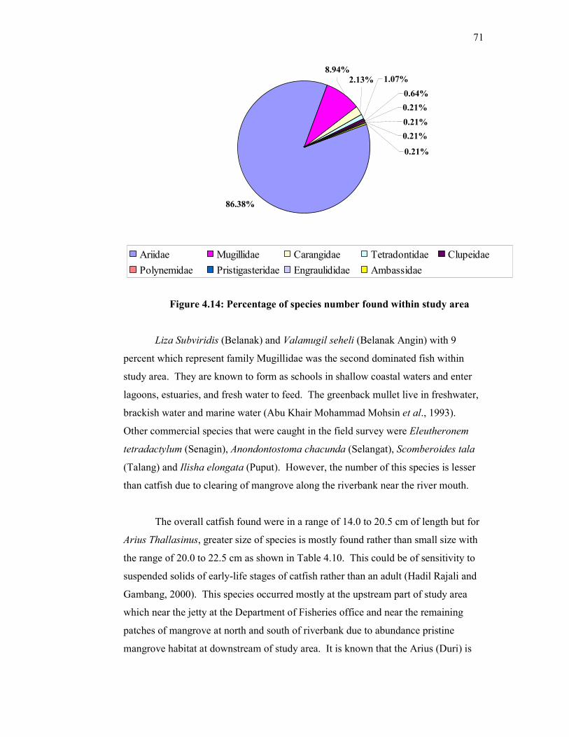
71

Figure 4.14: Percentage of species number found within study area

Liza Subviridis (Belanak) and Valamugil seheli (Belanak Angin) with 9

percent which represent family Mugillidae was the second dominated fish within

study area. They are known to form as schools in shallow coastal waters and enter

lagoons, estuaries, and fresh water to feed. The greenback mullet live in freshwater,

brackish water and marine water (Abu Khair Mohammad Mohsin et al., 1993).

Other commercial species that were caught in the field survey were Eleutheronem

tetradactylum (Senagin), Anondontostoma chacunda (Selangat), Scomberoides tala

(Talang) and Ilisha elongata (Puput). However, the number of this species is lesser

than catfish due to clearing of mangrove along the riverbank near the river mouth.

The overall catfish found were in a range of 14.0 to 20.5 cm of length but for

Arius Thallasinus, greater size of species is mostly found rather than small size with

the range of 20.0 to 22.5 cm as shown in Table 4.10. This could be of sensitivity to

suspended solids of early-life stages of catfish rather than an adult (Hadil Rajali and

Gambang, 2000). This species occurred mostly at the upstream part of study area

which near the jetty at the Department of Fisheries office and near the remaining

patches of mangrove at north and south of riverbank due to abundance pristine

mangrove habitat at downstream of study area. It is known that the Arius (Duri) is

86.38%

1.07%

0.21%

0.21%

0.21%

0.21%

0.64%

2.13%

8.94%

Ariidae Mugillidae Carangidae Tetradontidae Clupeidae

Polynemidae Pristigasteridae Engraulididae Ambassidae

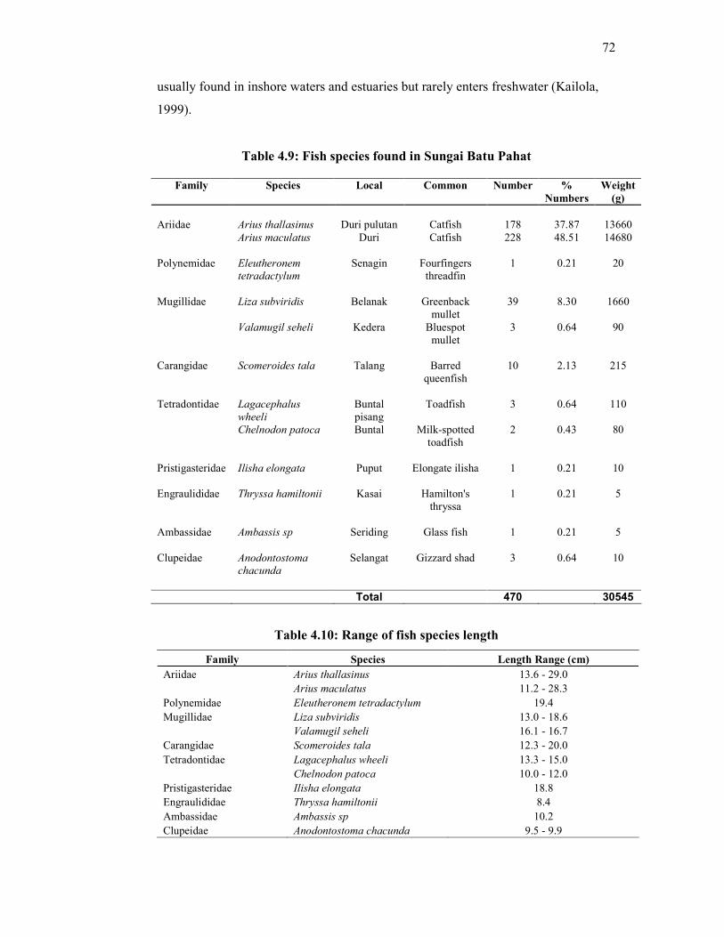
72

usually found in inshore waters and estuaries but rarely enters freshwater (Kailola,

1999).

Table 4.9: Fish species found in Sungai Batu Pahat

Table 4.10: Range of fish species length

Family Species Length Range (cm)

Ariidae Arius thallasinus 13.6 - 29.0 Arius maculatus 11.2 - 28.3 Polynemidae Eleutheronem tetradactylum 19.4 Mugillidae Liza subviridis 13.0 - 18.6 Valamugil seheli 16.1 - 16.7 Carangidae Scomeroides tala 12.3 - 20.0 Tetradontidae Lagacephalus wheeli 13.3 - 15.0 Chelnodon patoca 10.0 - 12.0 Pristigasteridae Ilisha elongata 18.8 Engraulididae Thryssa hamiltonii 8.4 Ambassidae Ambassis sp 10.2 Clupeidae Anodontostoma chacunda 9.5 - 9.9

Family Species Local Common Number %

Numbers

Weight

(g)

Ariidae Arius thallasinus Duri pulutan Catfish 178 37.87 13660 Arius maculatus Duri Catfish 228 48.51 14680 Polynemidae Eleutheronem

tetradactylum

Senagin Fourfingers threadfin

1 0.21 20

Mugillidae Liza subviridis Belanak Greenback

mullet 39 8.30 1660

Valamugil seheli Kedera Bluespot mullet

3 0.64 90

Carangidae Scomeroides tala Talang Barred

queenfish 10 2.13 215

Tetradontidae Lagacephalus

wheeli

Buntal pisang

Toadfish 3 0.64 110

Chelnodon patoca Buntal Milk-spotted toadfish

2 0.43 80

Pristigasteridae Ilisha elongata Puput Elongate ilisha 1 0.21 10 Engraulididae Thryssa hamiltonii Kasai Hamilton's

thryssa 1 0.21 5

Ambassidae Ambassis sp Seriding Glass fish 1 0.21 5 Clupeidae Anodontostoma

chacunda

Selangat Gizzard shad 3 0.64 10

Total 470 30545

73

Compared to WQI for Sungai Batu Pahat which is Class III at upstream and

decrease to Class IV at middle stream, it is not surprisingly about the dominance of

catfish because bottom-dwelling fish species like the catfish is tolerant to suspended

solids and low water quality (Hadil Rajali and Gambang, 2000). Moreover,

according to Kailola (1999), catfish was considered as commercial fish and occurs

often in schools form. Small crabs, mollusk and small fishes are become dietary for

catfish.

For other foremost commercial fish, the water quality of this estuaries may

effect their population and habitat which implied by number of this species were

caught in study area because they are not in tolerant fish type. The main reason for

existing of this juvenile species (range of 10.0 to 20.0 cm) is because of patches of

mangrove that still remain along the riverbank. For Eleutheronema tetradactylum

(Senangin), adult fish length may reach over than 50.0 cm. Marine fish and low

commercial value fish such as Lagacephalus lunaris (Buntal pisang) and Chelnodon

patoca (Buntal) also enters this estuaries even only 5 numbers of them. Meaning

that, the water quality at Sungai Batu Pahat still can support marine fish. But for

juveniles’ fish, they may enter mangrove and rice field. They take small algae,

diatoms and benthic detrital material as feeding (Harrison and Senou, 1997).

The size and length distribution of the species within study area shows a

normal and stable population of predominantly young and adult fishes. However, the

length of the species found within study area is considered small because, the

greenback mullet’s length may reach to 40 cm (Harrison and Senou, 1997). This is

regarding to decreasing of mangrove area for them to feed. Even though the water

quality within study area not in ‘health’ status for most commercial species, but the

mangrove remaining along the riverbank would be act as shelter and breeding area.

It is true that, the class III of water quality provided by DOE (1986) may support

abundance of tolerant fish such as Arius. However, there still have juvenile

commercial fish such as Eleutheronem tetradactylum (Senagin), Anondontostoma

chacunda (Selangat), Scomberoides tala (Talang) and Ilisha elongata (Puput) shows

that, fish species does not rely on water quality alone but also rely on breeding and

feeding area; mangrove (Alfaro, 2004; Cheevaporn and Menasveta 2003; Kathiresan

and Bingham, 2001; Nagelkerken et al., 1999; Gilbert and Janssen 1996).

74

4.7 Phytoplankton Analysis

The phytoplanktons are one of the initial biological components, from which

energy is transferred into higher organisms through food web. Biomass and

production of phytoplankton of various sizes are important factors, which regulate

the availability and diversity of organisms at higher trophic levels.

Table 4.11: Phytoplankton taxa during high tide

Stations Upstream Middle stream Downstream

Bacillariophyceae Chaetoceros sp. √ √ √ Thalassionema nitzschiodes √ √ √ Thalassiothrix frauenfeldii - - √ Biddulphia sp. √ √ √ Biddulphia sinensis √ √ √ Fragilaria sp. - - - Dithylium sol √ - √ Dithylium brightwellii √

Nitzschia longgisima √ √ √

Nitzschia sigma √ √ √

Nitzschia sp. - √ √

Pleurosigma sp. √ √ √

Navicula sp. √ √ √

Closterium sp. - - - Codonella aspera - - - Codonella americana - - - Codonella sp. - √ √

Tintinnopsis sp. √ √ √

Flavella sp. √ √ √

Xystonella lohmanni - - √

Ethmodiscus sp. √ - - Coscinodiscus lineatus - √ √

Cosconidiscus sp. √ √ √

Triceratium √ √ √

Rhizosolenia sp. √ √ √

Hemialus sp. √ √ √

Skeletonema costatum √ √ √

Guinardia sp. √ √ - Spyrogyra sp. - - - Leptocylindrus danicus - - - Dinophyceae Ceratium sp. √ √ √ Total Species 19 20 23

75

The dominant phytoplanktons in Sungai Batu Pahat are Bacillariophyceae or

diatom and Dinophyceae (dinoflagellates) during high tide (Table 4.11) and only

Bacillariophyceae were found during low tide (Table 4.12). Khiteka et al. (1996)

also found out that diatoms and dinoflagellates is dominant phytoplankton in Bay.

Phytoplanktons have direct relationship with tides, strength of the current and

direction of flows (Balasubramaniam, 2002). Bacillariophyceae species such as

Navicula and Spirogyra are seen only during low tide where the freshwater influence

in the biotopes.

Table 4.12: Phytoplankton taxa during low tide

Stations Upstream Middle stream Downstream

Bacillariophyceae Chaetoceros sp. √ √ √ Thalassionema nitzschiodes - - - Thalassiothrix frauenfeldii - - - Biddulphia sp. √ √ √

Biddulphia sinensis √ √ √

Fragilaria sp. √ √ - Dithylium sol - - - Dithylium brightwellii - - - Nitzschia longgisima - - - Nitzschia sigma - - - Nitzschia sp. √ √ - Pleurosigma sp. √ √ √

Navicula sp. √ - √

Closterium sp. √ √ - Codonella aspera - - √ Codonella americana - - √

Codonella sp. - - √

Tintinnopsis sp. √ √ √

Flavella sp. - - √ Xystonella lohmanni - - √

Ethmodiscus sp. - - - Coscinodiscus lineatus - - √

Cosconidiscus sp. - √ √

Triceratium - - √

Rhizosolenia sp. - √ - Hemialus sp. - - - Skeletonema costatum √ √ √ Guinardia sp. - - - Spyrogyra sp. - √ √ Leptocylindrus danicus - √ - Dinophyceae Ceratium sp. - - - Total Species 10 13 16

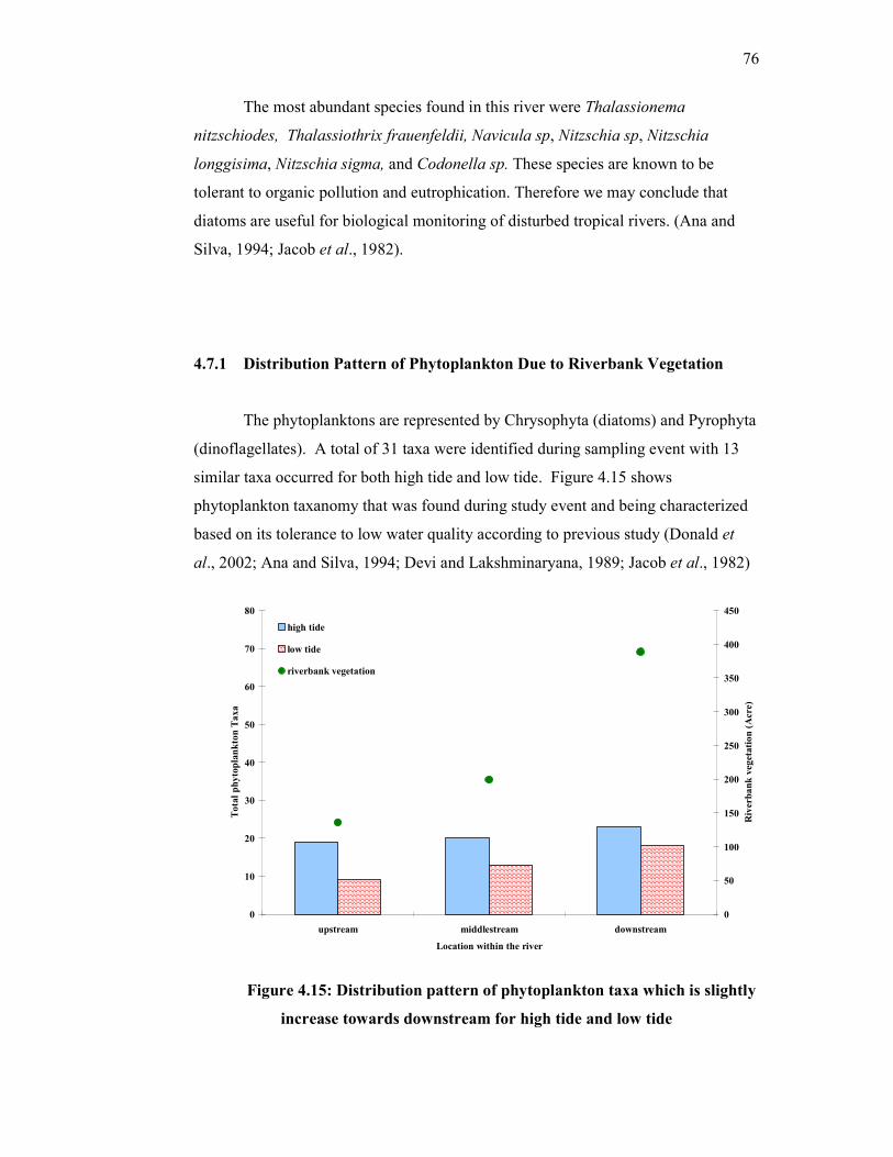
76

The most abundant species found in this river were Thalassionema

nitzschiodes, Thalassiothrix frauenfeldii, Navicula sp, Nitzschia sp, Nitzschia

longgisima, Nitzschia sigma, and Codonella sp. These species are known to be

tolerant to organic pollution and eutrophication. Therefore we may conclude that

diatoms are useful for biological monitoring of disturbed tropical rivers. (Ana and

Silva, 1994; Jacob et al., 1982).

4.7.1 Distribution Pattern of Phytoplankton Due to Riverbank Vegetation

The phytoplanktons are represented by Chrysophyta (diatoms) and Pyrophyta

(dinoflagellates). A total of 31 taxa were identified during sampling event with 13

similar taxa occurred for both high tide and low tide. Figure 4.15 shows

phytoplankton taxanomy that was found during study event and being characterized

based on its tolerance to low water quality according to previous study (Donald et

al., 2002; Ana and Silva, 1994; Devi and Lakshminaryana, 1989; Jacob et al., 1982)

Figure 4.15: Distribution pattern of phytoplankton taxa which is slightly

increase towards downstream for high tide and low tide

0

10

20

30

40

50

60

70

80

upstream middlestream downstream

Location within the river

Total phytoplankton Taxa

0

50

100

150

200

250

300

350

400

450

Riverbank vegetation (Acre)

high tide

low tide

riverbank vegetation

77

As shown in Figure 4.15, for high tide, there was 25 taxa occurred with the

distribution of phytoplankton 19 taxa at upstream, 20 taxa at middle stream and 23

taxa at downstream. Only 16 taxa were recognized to be at entire stream. While for

low tide, only 21 taxa were identified with 10 taxa (upstream), 13 taxa (middle

stream) and 16 taxa (downstream). There were 6 similar taxa identified within study

area. During high tide, total taxon of phytoplankton was found higher compared to

low tide event which dominated by Biddulphia spp and Chaetoceros spp. The

presence of diatoms, such as Chaetoceros spp., Thalassiosira spp., and Biddulphia

spp. is related to good quality water (Devi and Lakshminaryana, 1989) and most

common community found at warm water (Jacob et al., 1982).

Based on dissolved oxygen concentration during high tide, it showed an

acceptable level for aquatic life (>2 mg/L) (McCaull and Crossland, 1974) rather

than during low tide which is likely to have less than 2 mg/L except at downstream

(average of 5.25 mg/L). Other reason could be regarding to nutrient supply and light

ability which become an essential component for their productivity (Hoai et al.,

2006; Effler et al., 1991; Delizo et al., 2005). Injection of coastal water to estuaries

would be the main reason of increasing taxa during high tide. At mid high tide, the

concentrations of chlorophyll (associated with low levels of degraded pigments)

were higher than the concentrations (associated with a higher load of degraded

pigments) seen at mid low tide (Hoai et al., 2006). Chlorophyll was recognized to

identify the existing phytoplankton on water bodies (Tarim, 2002; Harris and

Piccinin, 1983).

Phytoplankton during low tide was much lower than high tide could be due to

lack of penetration of light to water column because of higher turbidity (Rao et al.,

1982). It is well known that, the low penetration of light into the water column

(rarely surpassing 10 cm) (Hoai et al., 2006) and anoxic condition (Ahsen et al.,

2006) does not allow a significant increase in phytoplankton productivity. Beside,

the decreasing of phytoplankton taxon during low tide was corresponding to

competition for nutrients with bacteria even there are nutrient supply from mangrove,

did not influence growth any further (Capo et al., 2005) and part of nutrient is used

to sustain zooplankton biomass (Khiteka et al., 1996).

78

Biddulphia spp and Codonella sp was identified to always present taxa during

low tide and it can be concluded that water quality of Sungai Batu Pahat still in good

condition and may support the high demanding phytoplankton such as Biddulphia

spp which rarely found in polluted water. Total phytoplankton was seen to be

increased towards downstream due to increasing of riverbank vegetation (main

supplier to their productivity) as well as imported nutrient from Strait of Malacca

water. While tidal change appears to determine the distribution pattern of

phytoplankton.

4.7.2 Distribution Pattern of Phytoplankton Due to Dissolved Oxygen

Phytoplanktons that were identified consist of two families which are diatom

and dinoflagellates. Diatoms are harmless and dinoflagellates that found in this

study were non-toxic species. During high tide and low tide, phytoplankton taxa

were increase with increasing of dissolved oxygen as shown in Table 4.13. The

decreasing taxa during low tide because of effluent discharge from tributaries such as

phosphorus from agriculture activities and quarry activites, and heavy metal from

urban area. Phytoplankton assemblage is sensitive to phosphorus and heavy metal

enrichment (Kitheka et al., 2000). Phytoplanktons that are not limited by nitrogen or

phosphorus are likely to have nutrient ratios of approximately 106C:16N:1P on a

molar basis (Donald et al., 2002). All phytoplankton found at study area were

tolerant to organic pollution.

Table 4.13: Phytoplankton taxa as compared to DO concentration


Variables Upstream Middle stream Downstream

DO

(mg/L)

Phytoplankton

(taxa)

DO

(mg/L)

Phytoplankton

(taxa)

DO

(mg/L)

Phytoplankton

(taxa)

High tide 3.02 19 3.78 20 5.34 23

Low tide 2.04 9 2.06 13 3.94 18 Riverbank vegetation (acre) 135.72 199.21 388.85

79

4.7.3 Distribution Pattern of Phytoplankton Due to pH

According to Weisse and Stadler (2006), pH is an important physicochemical

environmental parameter affecting ciliate species composition and species richness.

However, an experimental laboratory investigation of the pH reaction norm of

common species is still lacking. From Table 4.14, phytoplankton species were

increase as pH increase even the water still considered as acidic waters. As the pH

change, the species also change. Huang et al. (2003) identified that the

phytoplankton amount was highest in autumn, as was the pH value. When the pH

decreases, dinoflagellates tend to dominance. Dinoflagellate is toxic algae that could

harm fish and grazer (Rao et al., 1982) in toxic condition.

Table 4.14: Phytoplankton taxa as compared to pH



pH

Phytoplankton

(taxa) pH

Phytoplankton

(taxa) pH

Phytoplankton

(taxa)

High tide 3.4 19 4.45 20 5.34 23


4.8 Zooplankton Analysis

Zooplankton is significant food for fish and invertebrate predators and they

graze heavily on algae, bacteria, protozoa, and other invertebrates (Victor et al.,

2006). Table 4.15 shows numbers of zooplankton the present in Sungai Batu Pahat

in unit ind/m3 during high tide while during low tide is shown in Table 4.16.

The indices of species richness, Margalef index (D) and Shannon-Weiner index

(H’) with higher value showed that composition of zooplankton was more diverse at

the downstream stations than at the upstream stations (see Appendix B). The

evenness Pielou’s index (J’) also showed that the community of zooplankton in the

adjacent coastal waters (J’= 0.43) during low tides was constituted by various species

80

as compared to the river’s community which mainly dominated by rotifer. It can be

concluded that zooplankton species diversity and abundance at Sungai Batu Pahat is

mainly influenced by the sea and tides. Hoai et al. (2006) was identified rotifers,

copepods and cladoceran were dominant zooplankton during high tide and low tide

near the river mouth.

Table 4.15: Zooplankton during high tide in unit ind/m3

Taxa Upstream Middle stream Downstream

ROTIFERA Brachionus sp. 3391.7 7074.9 2118.6

CRUSTACEA Copepoda Copepod nauplius 36.7 184.5 1443.5

Calanoida Acartia sp. 0 5.7 747.9 Pontellidae copepodid 0 0 8.7 Pseudodiaptomus sp. 0 0 57.7 Parvocalanus sp. 0 0 60.4 Paracalanidae copepodid 0 0 113.3 Centropages sp. 0 0 34.9 Unidentified calanoid copepodid 0 16.2 0

Cyclopoida Oithona sp. 0 7.3 170.2 Cyclops sp. 23.2 76.6 95.2

Harpaticoida Euterpina sp. 0 3.6 0 Harpaticoid sp1 0 0 43.9

Decapoda Acetes protozoea 0 0 9.2 Lucifer mysis 0 0 8.7

Ostracoda 0 7.2 202.9

Cladoceran Moinodaphnia sp. 4.0 2.1 0

Cirripedia Cirripede nauplius 12.8 61.4 204.5

SARCOMASTIGOPHORA

(PROTOZOA) Tintinnopsis sp. 0 0 5.2 Favella sp. 32.7 43.2 245 Noctiluca sp. 108.6 235.1 1388.8 Total 3609.7 7717.6 6958.8

81

Table 4.16: Zooplankton during low tide in unit ind/m3

Taxa Upstream

Middle

stream Downstream

ROTIFERA Brachionus sp. 2911.6 6567.5 1700.2

CRUSTACEA Copepoda Copepod nauplius 0 12.8 19362.2

Calanoida Acartia sp. 0 0 7044.2 Pontellidae copepodid 0 0 1288.2 Pseudodiaptomus sp. 0 0 24305.0 Parvocalanus sp. 0 0 7337.5 Bestiolina sp. 0 0 14433.8 Paracalanus sp. 0 0 257.6 Paracalanidae copepodid 0 0 756.5 Eucalanus sp. 0 0 257.6 Temora sp. 0 0 257.6 Unidentified calanoid copepodid 0 0 16.5

Cyclopoida Oithona sp. 0 0 16895.6 Cyclops sp. 84.0 142.7 33.0

Harpaticoida Euterpina sp. 0 0 1408.8

Decapoda Acetes protozoea 0 0 257.6 Lucifer protozoea 0 0 2233.9 Lucifer sp. 0 0 704.4

Ostracoda 0 0 0

Cladoceran Anollela sp. 83.9 116.6 12.4 Moinodaphnia sp. 26.5 17.2 0

Cirripedia Cirripede nauplius 0 0 772.9

CHAETOGNATHA Sagitta sp. 0 0 772.9

CNIDARIA Leptomedusa (hydrozoa) 0 0 4.1

SARCOMASTIGOPHORA

(PROTOZOA) Tintinnopsis sp. 0 0 189.1 Favella sp. 0 0 257.6 Total 3106.1 6856.9 100559.6

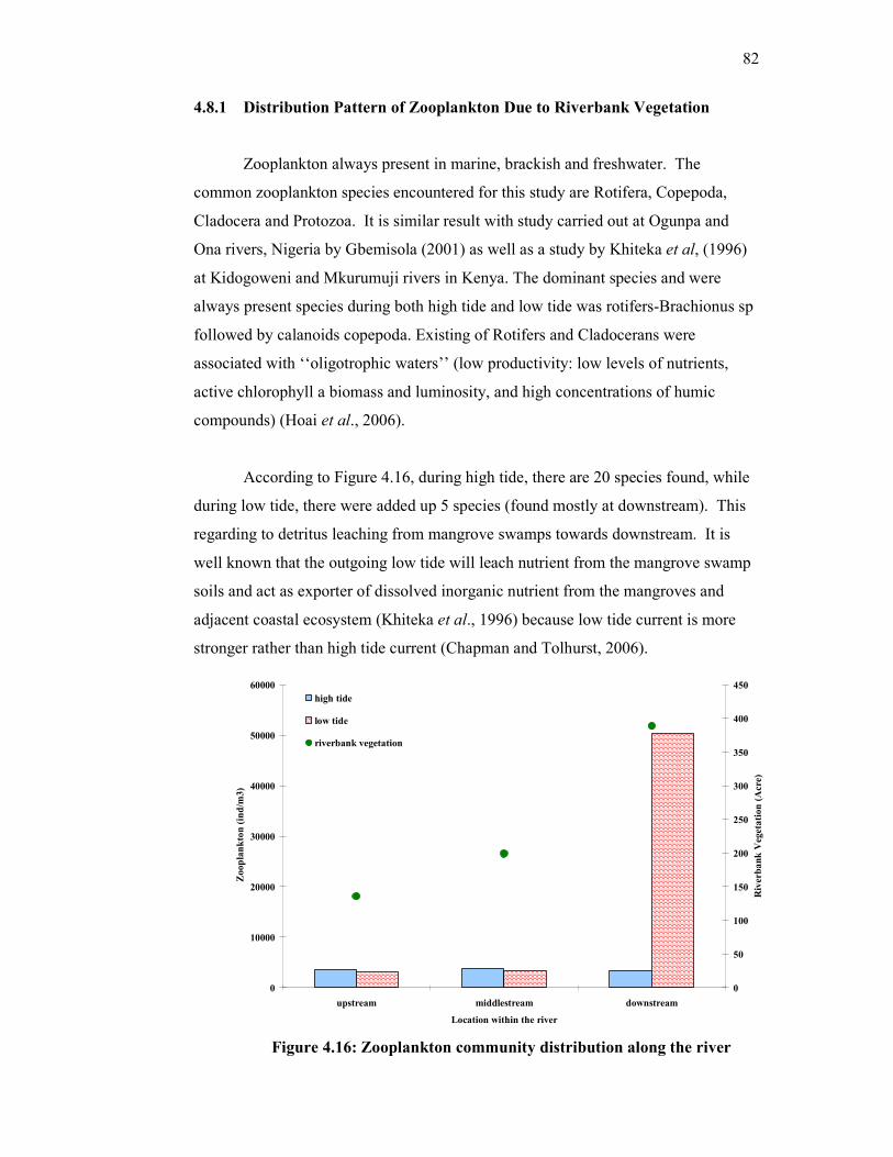
82

4.8.1 Distribution Pattern of Zooplankton Due to Riverbank Vegetation

Zooplankton always present in marine, brackish and freshwater. The

common zooplankton species encountered for this study are Rotifera, Copepoda,

Cladocera and Protozoa. It is similar result with study carried out at Ogunpa and

Ona rivers, Nigeria by Gbemisola (2001) as well as a study by Khiteka et al, (1996)

at Kidogoweni and Mkurumuji rivers in Kenya. The dominant species and were

always present species during both high tide and low tide was rotifers-Brachionus sp

followed by calanoids copepoda. Existing of Rotifers and Cladocerans were

associated with ‘‘oligotrophic waters’’ (low productivity: low levels of nutrients,

active chlorophyll a biomass and luminosity, and high concentrations of humic

compounds) (Hoai et al., 2006).

According to Figure 4.16, during high tide, there are 20 species found, while

during low tide, there were added up 5 species (found mostly at downstream). This

regarding to detritus leaching from mangrove swamps towards downstream. It is

well known that the outgoing low tide will leach nutrient from the mangrove swamp

soils and act as exporter of dissolved inorganic nutrient from the mangroves and

adjacent coastal ecosystem (Khiteka et al., 1996) because low tide current is more

stronger rather than high tide current (Chapman and Tolhurst, 2006).

Figure 4.16: Zooplankton community distribution along the river

0

10000

20000

30000

40000

50000

60000



Zooplankton (ind/m

3)

0

50

100

150

200

250

300

350

400

450

Riverbank Vegetation (Acre)

high tide

low tide


83

Other zooplankton encountered for this study were Decapoda , Cirripedia At

upstream and middle stream, for both tides, the zooplankton species were diverse and

well distribute but in different percentage. At upstream, there are 7 species with

average 3609.7 ind/m3, whereas average number of zooplankton is 3858.8 ind/m3

were found at middle stream with 12 species during high tide. For average number

of zooplankton low tide density at upstream and middle stream was evaluated of

3106.1 ind/m3 with 4 species involved and 3428.6 ind/m3 with 5 species,

respectively.

There was less 12 percent reduction of zooplankton density with less species

found during low tide for both upstream and middle stream because of human

activities such as quarry, settlement and heavy boat traffics with respect to mangrove

loss and less detritus. Zooplankton consumes bacteria and detritus as their nutrition

(Rougier et al., 2004). Beside, this could be due to food availability, spawning

patterns of different zooplankton groups and tidal rhythms (Khiteka et al., 2006) and

their percentages were independent of the tidal cycles (Rougier et al., 2004).

At downstream, the abundance of zooplankton during low tide with 24

species (average of 50279.8 ind/m3) compared to high tide with only 18 species

(average of 3479.4 ind/m3) with 19.7 percent rotifers reduction. The number of

rotifers during high tide and low tide is 1700.2 ind/m3 and 2118.6 ind/m3,

respectively. According to Rougier et al, (2004), there are less 20 percent of rotifer

reduction between high tide and low tide period. The high in number of

zooplankton during low tide at downstream with respect to river mouth and

abundance of mangrove habitat which characterized by strong turbidity and high

amounts of organic detritus, the presence of bacteria and detritus could contribute to

the maintenance of this community (Rougier et al., 2004). Furthermore, the other

reason of abundance species at downstream during low tide could be the low salinity

water that outflow from freshwater during this period (Khiteka et al., 1996).

The existing of abundance copepods in Sungai Batu Pahat relating to water

quality which have acidic water (range 3-6) was common because copepods was

characterized as much hardier and strong motile than other zooplankton with their

tougher exoskeleton and longer and stronger appendages (Ramachandra et al., 2006).

84

This finding supported by Jha and Barat (2003) that, found abundance of copepods in

acidic pH of water bodies due to nature and other physicochemical factor.

The abundance of copepods relate to the stable condition of environment

(Das et al., 1996). Beside, it is well recognized that zooplankton is exists under a

wide range of environment, but there are many species are influenced by

temperature, dissolved oxygen, salinity and other physicochemical factors. For

example, rotifer is more sensitive to pollution rather than other groups of

zooplankton (Khan and Rao, 1981). However, Sungai Batu Pahat can be classified

as slightly polluted but abundance of rotifers found it most stream portion. Pandey et

al, (2004) found that there were negative correlation between rotifers and pH,

dissolved oxygen (DO) and turbidity while copepods showed negative correlation

with water temperature, nitrate and phosphate.

4.8.2 Distribution Pattern of Zooplankton Due to Dissolved Oxygen

Dissolved oxygen shows depletion during low tide at upstream with 20.5%,

45 % at middle stream and 26% at downstream. The depletion of DO concentration

resulting low water quality and only tolerant species may survive as shown in Table

4.17. At upstream, species that less tolerant will decrease during low tide and be

replaced by abundance of tolerant species which less in number during high tide.

Same thing goes at middle stream, which some species that exist during high tide,

suddenly disappeared during low tide.

Table 4.17: Zooplankton numbers as compared to DO concentration



DO

(mg/L)

Zooplankton

(ind/m3)

DO

(mg/L)

Zooplankton

(ind/m3)

DO

(mg/L)

Zooplankton

(ind/m3)

High tide 3.02 3609.7 3.78 3858.8 5.34 3479.4

Low tide 2.4 3106.1 2.06 3428.6 3.94 50279.8 Riverbank vegetation (acre) 135.72 199.21 388.85

85

This species shows water quality during low tide much polluted. At

downstream, however, zooplankton species increase with decreasing of DO

concentration. This associated to rapid increasing of tolerant species with abundance

of nutrient leaching from riverbank vegetation and freshwater. According to Victor

et al. (2006), low DO will lead to decreasing of zooplankton taxa richness, however

increase the taxon or taxa that tolerant to low DO.

4.8.3 Distribution Pattern of Zooplankton Due to pH

There is little direct evidence of low pH induced changes in the total

zooplankton biomass. However, it is clear that species composition may vary as a

result of the different tolerances of species to low pH values. From Table 4.18,

zooplankton assemblages are varies with respect to increasing of pH value. Changes

in zooplankton may also alter the pressure due to predation on phytoplankton, thus

affecting species composition. In addition, sudden variations of pH, typical of

weakly buffered systems can shift to species that more tolerant to it.

Table 4.18: Zooplankton numbers as compared to pH



pH

Zooplankton

(ind/m3) pH

Zooplankton

(ind/m3) pH

Zooplankton

(ind/m3)

High tide 3.4 3609.7 4.45 3858.8 5.34 3479.4

Low tide 3.54 3106.1 3.87 3428.6 5.78 50279.8 Riverbank vegetation (acre) 135.72 199.21 388.85

4.9 Macrobenthos Analysis

Table 4.19 and Table 4.20 show type of macrobenthos that had been caught

during high tide and low tide respectively. Number and types of benthic

86

communities were absolutely low due to human disturbance but still exist as existing

of detritus that acts as food and habitat provided by mangrove.

Table 4.19: Benthic macroinvetebrates within study area during high tide

Table 4.20: Benthic macroinvetebrates within study area during low tide

4.9.1 Distribution Pattern of Macobenthos Due to Riverbank Vegetation

Microinvertebrate or also known as macrobentos found in Sungai Batu Pahat

was poor diversity. According to Figure 4.17, during high tide, no macrobenthos

species was found at upstream and middle stream but polycate (4 Nereis sp and 4

Polycate sp 1) and primitive bivalves (6 Yoldia) was identified at downstream with

Stream Benthos

Total

No. Notes

Downstream Polychate : Nereis sp. 4 Fragments of bivalves, gastropods, oysters,

: Polychate sp. 1 Bivalves : Yoldia

1 6

detritus as well as presence of charcoal/ carbon

Middle stream

0

Sand, Twigs and broken branches, unidentified fruits, seeds, sea grass, weeds and fragment of plants

Upstream

0

Root, grass and sand

Stream Benthos

Total

No. Notes

Downstream

Polychate : Sabellidae :Polychate sp. 2 :Nereis sp.

1 1 4

Fragments of bivalves, gastropods, oysters and detritus as well as weeds.

Middle stream Gastropod: Nassarius sp. 3 Detritus, leaves and fragments of plants Diopatra 1 Polychate : Nereis sp. 2

Upstream

Polychate : Nereis sp.

1

Clay substrate, detritus, muddy substrate and fragments of bivalves

87

fragments of bivalves, gastropods and oyster was found. The substrate at

downstream at the river mouth is dark muddy and oily probably due to discharges or

spillages from vessels entering and exiting the river. The substrate is sandy at

downstream while at middle stream, the substrate is sandy with and rocky with

gravels that might have fallen of barges carrying gravel from the nearby quarry site.

Only fragments of plants and detritus were found at upstream and

downstream. During low tide, 1 polycate Nereis sp (upstream), and 2 Nereis sp

(middle stream) 1 polycate Sabellidae, 4 Nereis sp, 1 Polycate sp 2, 1 Diopatra and 3

Gastropod Nassarius sp (downstream) was found. The average value of total

macrobenthos during high tide and low tide were as follow, respectively; 0

(upstream), 0 (downstream), 5.5 (downstream) and 1 (upstream), 2 (upstream), 10

(downstream). The abundance of macrobenthos at downstream could be respond to

the great areas of riverbank vegetation and wide area.

Figure 4.17: Macrobenthos that found during study event which shows

low diversity during high tide and low tide

In general, the abundance of macrobenthos in the study area was relatively

low. This was probably due to the fact that the study area have been subjected to

0

2

4

6

8

10

12



Numbers of Macrobenthos

0

50

100

150

200

250

300

350

400

450

Riverbank Vegetation (Acre)

high tide

low tide


88

significant environmental alteration that may have lead to heavy disturbance and

unstable river bed. High number of marine traffic and barges carrying gravel from

the nearby quarry may have contributed to this condition. Polycates and bivalves

which mostly present species of macrobenthos within study area was not something

new because this species has highly tolerant to organic pollution (Ahsen et al., 2006;

Luoma and Cloern, 1980).

4.9.2 Distribution Pattern of Macrobenthos Due to Dissolved Oxygen

Macrobenthos that had been caught during study event was poor in number as

shown in Table 4.21. During high tide, even DO increase, no species were found at

upstream and downstream because, at upstream, the substrate is sand which always

no species present (Chindah and Braide, 2001). While at middle stream, sediment

was disturbed by sandy with and rocky with gravels that might have fallen of barges

carrying gravel from the nearby quarry site. At downstream, number of benthos

increasing due to muddy substrate and quality of food supplied.

Table 4.21: Numbers of macrobenthos as compared to DO concentration

During low tide, a few species that tolerant to low DO concentration were

found. This is because, during high tide, this species will burrow deep beneath the

surface to avoid them from flushing to downstream when low tide event occurred

(Chindah and Braide, 2001). They only emerged to bring down food and oxygen.

DO concentration not directly related to macrobenthos assemblage because, the

sediment had already disturbed by human activities. Most of species found in this

study were tolerant to low water quality.



DO

(mg/L)

Macrobenthos

(no)

DO

(mg/L)

Macrobenthos

(no)

DO

(mg/L)

Macrobenthos

(no)

High tide 3.02 0 3.78 0 5.25 5.5


89

Hypoxia and anoxia degrade bottom habitats through a wide suite of

mechanisms. Under conditions of limited oxygen at the bottom, rates of nitrogen and

phosphorous remineralization and sulfate reduction increase. The resulting

production of sulfide in combination with low oxygen can prove lethal to benthic.

Because benthic macrofauna serve as essential prey resources for demersal fishes,

sustained hypoxia can have significant trophic implications (Lin et al., 2006)

The poor diversity of benthic macroinvertebrate assemblages in Sungai Batu

Pahat generally because alteration of ecosystem structure and function in streams

through habitat homogenization, oxygen depletion, organic matter retention

decreasing, as well as ammonium and phosphate uptake velocity decreasing, that

shifts towards tolerant organisms (Thomas, 2004)

4.9.3 Distribution Pattern of Macrobenthos Due to pH

According to Table 4.22, macrobenthos community were less influenced by

pH value because the sediment of Sungai Batu Pahat was already disturbed by

human activities such as oil disposal and gravel that fallen from quarry nearby

(Simpson and Pedini, 1985). They added that, benthic activity in the water column

and sediment is primarily limited by the low availability of organic matter

characteristic of these ponds, and not so much by the low pH. Only the tolerant

species and a lot of bivalve fragment and detritus were found during study event.

Table 4.22: Numbers of macrobenthos as compared to pH



pH

Macrobenthos

(no) pH

Macrobenthos

(no) pH

Macrobenthos

(no)

High tide 3.4 0 4.45 0 5.34 5.5 Low tide 3.54 1 3.87 2 5.78 10 Riverbank vegetation (acre) 135.72 199.21 388.85

CHAPTER V

CONCLUSION

5.1 Conclusion

The study of water quality and biodiversity at Sungai Batu Pahat has

achieved its objectives. Water quality was analyzed by using DOE-WQI and was

found that, water quality at Sungai Batu Pahat during high tide and low tide was

consistent from upstream towards downstream with class III at upstream, down to

class IV at middle stream and eventually increase to class III at downstream. From

land use analysis, the fluctuating of water quality at Sungai Batu Pahat is strongly

related to human activities especially by untreated sewage and waste disposal from

urban area, settlement and barter-trades jetties.

While, since we go through to each parameter analysis, the most influence

parameter that causes the deteriorating of water quality to class IV at middle stream

for high tide and low tide are organic and inorganic matter which can be seen at

BOD and COD analysis. During high tide, water quality is much better rather than

during low tide due to mixing of coastal water and freshwater that resulting dilution.

During low tide, water quality much worst because of polluted water injected to

estuaries from tributaries.

Generally, the distribution of planktonic life and macroinvertebrates within

study area was tidal and mangrove dependent. Biodiversity was found abundance at

downstream and present with low number and species at upstream and downstream

91

probably because lands use activities. Biodiversity that mostly found within study

area is tolerant species to low dissolved oxygen concentration and pH.

Although physical and chemical variables are commonly used to determine

water quality, these parameters by themselves can only express the conditions of

water at the moment of sampling. On the other hand, biological monitoring can give

information about the water conditions for a longer period. From the analysis of

water quality and biodiversity at Sungai Batu Pahat, can be concluded that Sungai

Batu Pahat still can support the aquatic life such as fish, zooplankton, phytoplankton

and macrobenthos even though only the abundance of tolerant species appeared due

to slightly polluted river water classification. The abundance species of diatom in

Sungai Batu Pahat indicates that mangrove in this area are in a good health (Prepas

and Charette, 2003; Holguin et al., 2005)

Furthermore, high commercial fish and demanding species (require high

quality of water to survive) such as a juvenile gizzard shad, rotifers zooplankton and

Biddulphia sp phytoplankton was found within study area were strongly support this

finding. Although the WQI shows low quality of water, the existing riverbank such

as mangrove and tidal changes play an important role in determining the abundance

of quality food and safety home for aquatic life. The decreasing of riverbank

vegetation in the future may reduce the present of aquatic life in Sungai Batu Pahat

This finding was similar to study that made by Hajisame and Chou (2003) at

Johor Strait, Peninsular Malaysia. They conclude that, although the Johor Strait is

heavily impacted, there are still some tolerant habitats that remain because of

existing patches of mangrove as well as act as an important ecosystem for a diverse

assemblage of juveniles and small-sized fish species.

5.2 Recommendation

There are a few measures which can be taken in order to improve the quality

of Sungai Batu Pahat in term of water and biodiversity such as:

92

(i) Relocated the squatters along the riverbank to another proper place to

stay;

(ii) Governments should issue and enforce legislation to control industrial

activities in the coastal zone. Such legislation would profitably be

accompanied by monitoring and should be enforced by authorized

government agencies;

(iii) Enhance the total area covered by mangroves. The easiest and least

expensive way to achieve this goal is to assist natural mangrove

colonization in sheltered coastal segments by providing or enhancing

seedling fluxes to the area, protecting seedlings from herbivory and

increasing propagule retention time with artificial shelters.

In order to improve the accuracy as well as the effectiveness of this study,

there are a few recommendation that should been follow such as;

(i) Added more sampling station and water quality parameter such as heavy

metals and phosphate;

(ii) Sampling event should be made longer period to identify the actual

distribution of planktonic life and benthic macroinvertebrates;

(iii) Detail study should be made on mangrove activities in order to achieved

actual nutrient contributor to biota growth.

REFERENCES

Abu Khair Mohammad Mohsin, Mohd. Azmi Ambak and Muhamad Nasir Abdul

Salam. (1993). “Malay, English, and Scientific Names of the Fishes of

Malaysia.” Faculty of Fisheries and Marine Science, Universiti Pertanian

Malaysia, Selangor Darul Ehsan, Malaysia: Occasional Publication No. 11.

Ahsen, Y., Erdogan, O.I., Yilmaz, N., Yilmaz, A.A. and Tas, S. (2006). “Changes in

Biodiversity of the Extremely Polluted Golden Horn Estuary Following the

Improvements in Water Quality.” Marine Pollution Bulletin. 52. 1209-1218.

Alfaro, A.C. (2004). “Benthic Macro-Invertebrate Community Composition within a

Mangrove/Seagrass Estuary in Northern New Zealand.” Estuarine, Coastal

and Shelf Science. 66. 97-110.

Alongi, D.M. (1986). “Quantitative Estimates of Benthic Protozoa in Tropical

Marine Systems Using Silica Gel: A Comparison of Methods.” Estuarine,

Coastal and Shelf Science. 4(23). 443-450.

Alongi, D.M. , Sasekumar A., Tirendia, F. and Dixona, P.(1998). “The Influence of

Stand Age on Benthic Decomposition and Recycling Of Organic Matter in

Managed Mangrove Forests of Malaysia.” Journal of Experimental Marine

Biology and Ecology. 225. 197-218.

Alongi, D.M., Chong, V.C., Dixona, P., Sasekumar, A. and Tirendia, F. (2003). “The

Influence of Fish Cage Aquaculture on Pelagic Carbon Flow and Water

Chemistry in Tidally Dominated Mangrove Estuaries of Peninsular

Malaysia.” Marine Environmental Research. 55. 313–333.

94

Alongi, D.M., Tirendi, F. and Trott, L.A. (1999). “Rates and Pathways of Benthic

Mineralization in Extensive Shrimp Ponds of the Mekong Delta, Vietnam.”

Aquaculture.175. 269–292.

Alonso, E., Santos, A., Callejon, M. and Jimenez, J.C. (2003). “Speciation as a

Screening Tool for the Determination of Heavy Metal Surface Water

Pollution in the Guadiamar River Basin.” Chemosphere. 56. 561–570.

Ana, M. and Silva, B. (1994). “The Use of Water Chemistry and Benthic Diatom

Communities for Qualification of a Polluted Tropical River in Costa Rica.”

Institute of Botanik, University Innsbruck, Innsbruck, Austria.

APHA (2000). “ Standard Methods for the Examination of Water and Wastewater.”

21st Edition. Washington, DC: American Public Health Association.

Ardebili, O., Didar, P. and Soheilinia, S. (2006). “Distribution and Probable Origin

of Heavy Metals in Sediments of Bakhtegan Lake, Fars Province, Iran.”

Goldschmidt Conference Abstracts. Iran.

Ashkan, F. (2000). “Magnitud and Extent of the Metal Contamination in Hudson

River Estuary Surficial Bottom Sediment.” The City University of New York:

PhD Thesis. 61-215.

Ashton, E.C. (2002). “Mangrove Sesarmid Crab Feeding Experiments in Peninsular

Malaysia.” Journal of Experimental Marine Biology and Ecology. 273. 97–

119.

Ashton, E.C. and Macintosh, D.J. (2002). “Preliminary Assessment of the Plant

Diversity and Community Ecology of the Sematan Mangrove Forest,

Sarawak, Malaysia.” Forest Ecology and Management. 160. 111-129.

Azrina, M.Z., Yap, C.K., Rahim Ismail, A., Ismail, A., dan Tan, S.G. (2006).

“Anthropogenic Impacts on the Distribution and Biodiversity of Benthic

95

Macroinvertebrates and Water Quality of the Langat River, Peninsular

Malaysia.” Ecotoxicology and Environmental Safety. 64. 337-347.

Bahadir, T., Bakan, G., Altas, L. and Buyukgungor, H. (2005). “The Investigation of

Lead Removal by Biosorption: An Application at Storage Battery Industry

Wastewaters.” Ecotoxicology and Environmental Safety.

Balasubramaniam, T. (2002). “Mangroves of India.” Annamalai University Tamil

Nadu, India.

Bano, N., Nisa, M., Khan, N., Saleem, M., Harrison, P.J., Ahmed, S.I., Azam, F.

(1997). “Significance of Bacteria in the Flux of Organic Matter in the Tidal

Creeks of the Mangrove Ecosystem of the Indus River Delta, Pakistan.”

Marine Ecological Program. 157. 1– 12.

Bayen, S., Wurl, O., Karuppiah, S., Sivasothi, N., Lee H. K. and Obbard, J.P. (2004).

“Persistent Organic Pollutants in Mangrove Food Webs in Singapore.”

Chemosphere .61. 303–313.

Bouillon, S., Koedamb, N., Baeyensa, W., Satyanarayanac, B. and Dehairsa, F.

(2002). “Selectivity of Subtidal Benthic Invertebrate Communities for Local

Microalgal Production in an Estuarine Mangrove Ecosystem during the Post-

Monsoon Period.” Journal of Sea Research. 51. 133– 144.

Butcher, J.T., Stewart P.M. and Simon, T.P. (2003). “A Benthic Community Index

for streams in the Northern Lakes and Forests Ecoregion.” Ecological

Indicators. 3. 181–193.

Capo, S., Sottolichio, A., Brenon, I., Castaing, P. and Ferry, L. (2005). “Morphology,

Hydrography and Sediment Dynamics in a Mangrove Estuary: The Konkoure

Estuary, Guinea.”Marine Geology .23. 199-215.

96

Carlos, S.L. and Marin, A. (2006). “Benthic Recovery during Open Sea Fish

Farming Abatement in Western Mediterranean, Spain.” Marine

Environmental Research. 62. 374–387.

Cech, T.V (2003). “Principles of Water Resources: History, Development,

Management, and Policy.” United State of America: John Wiley & Sons, Inc.

Chapman, M.G. and Tolhurst, T.J. (2006). “Relationships between Benthic

Macrofauna and Biogeochemical Properties of Sediments at Different Spatial

Scales and Among Different Habitats in Mangrove Forests.” Jounal of

Experimental Marine Biology and Ecology .343. 96-109.

Cheevaporn, V. and Menasveta, P. (2003). “Water Pollution and Habitat Degradation

in the Gulf of Thailand.” Marine Pollution Bulletin. 47. 43–51.

Chen, C.W., Kao, C.M, Chen, C.F. and Dong, C.D. (2006). “Distribution and

Accumulation of Heavy Metals in the Sediments of Kaohsiung Harbor,

Taiwan.” Chemosphere. 66. 1431–1440.

Chindah, A.C. and Braide, S.A. (2001). “Meiofauna Occurrence and Distribution in

Different Substrate Types of Bonny Brackish Wetland of the Niger Delta.”

Journal of Applied Sciences & Environmental Management. 33-41.

Chipman, W.A, J (1934). “The Role of pH in Determining the Toxicity of

Ammonium Compounds”. University of Missouri, Columbia: Ph.D. Thesis.

Christensen, B. (1976). “Biomass and primary production of Rhizophora apiculata

Bl. in a mangrove in southern Thailand.” Aquatic Botany. 4. 43-52.

Christensen, B. and Andersen, S.W. (1976). “Seasonal Growth of Mangrove Trees in

Southern Thailand.:The phenology of Rhizophora apiculata Bl.” Aquatic

Botany. 3. 281-286.

97

Clough, B., Tan, D.T., Phuong, D.X. and Buu, D.C. (2000). “Canopy Leaf Area

Index and Litter Fall in Stands of the Mangrove Rhizophora Apiculata of

Different Age in the Mekong Delta, Vietnam.” Aquatic Botany. 66. 311–320.

Colombini, I., Berti, R., Ercolini, A., Nocita, A. and Chelazzi, L. (1994).

“Environmental Factors Influencing the Zonation and Activity Patterns of a

Population of Periophthalmus Sobrinus Eggert in a Kenyan Mangrove.”

Journal of Experimental Marine Biology and Ecology. 190. 135-149.

Corami, A., Mignardi, S. and Ferrini, V. (2006). “Copper and Zinc Decontamination

from Single- And Binary-Metal Solutions Using Hydroxyapatite.” Journal of

Hazardous Materials.

Corbitt, R.A. (1999). “Standard Handbook of Environmental Engineering.2nd Ed.

New York: McGraw Hill.

Costanzo, S.D., O’Donohue, M.J. and Dennison, W.C. (2004). “Assessing the

Influence and Distribution of Shrimp Pond Effluent in a Tidal Mangrove

Creek in North-East Australia.” Marine Pollution Bulletin. 48. 514–525.

Dalman, O., Demirak, A. and Balcı, A. (2004). “Determination of Heavy Metals (Cd,

Pb) and Trace Elements (Cu, Zn) in Sediments and Fish of the Southeastern

Aegean Sea (Turkey) by Atomic Absorption Spectrometry.” Food Chemistry.

95. 157–162.

Das, P.K., Micheal, R.G., and Gupta, A. (1996). “Zooplankton Community Structure

of Lake Tasek, a Tectonic Lake in Garo hills, India.” Tropical Ecology.

37(2). 257-263.

Davide, V., Pardos, M., Diserens, J., Ugazio, G., Thomas, R. and Dominik, J. (2002).

“Characterisation of Bed Sediments and Suspension of the River Po (Italy)

During Normal and High Flow Conditions.” Water Research. 37. 2847–2864.

98

Delizo, L., Walker, O.S.J. and Hall, J. (2005). “Taxonomic Composition and Growth

Rates of Phytoplankton Assemblages at the Subtropical Convergence East of

New Zealand.” Virginia Institute of Marine Sciences. 3. 32-54.

Demirak, A., Yilmaz, F., Tuna, A.L. and Ozdemir, N. (2005). “Heavy Metals in

Water, Sediment and Tissues of Leuciscus Cephalus from a Stream in

Southwestern Turkey.” Chemosphere. 63. 1451–1458.

Department of Fisheries. (2005). Annual Report of Fisheries at Johor for 2005.

Department of Fisheries, Malaysia.

Desa, E., Zingde, M.D., Vethamony, P., Babu, M.T., D’Sousa, S.N. and Verlecar,

X.N. (2005). “Dissolved Oxygen––A Target Indicator in Determining Use of

the Gulf of Kachchh Waters.” Marine Pollution Bulletin. 50. 73–79.

Desai, K.N. and Untawale, A.G. (2002). “Sand Dune Vegetation of Goa:

Conservation and Management.” Botanical Society of Goa, India.101 pp.

Devi, J.S. and Lakshminaryana. J.S.S. (1989). “Studies on the Phytoplankton and the

Water Quality of Malpaque Bay Prince Edward Island Canada.” Proc N S

Institution Science .39. 39 – 50.

DOE (1986). “Classification of Malaysian Rivers.” Department of Environment,

Malaysia.

DOE (1986). “Water Quality Criteria and Standards for Malaysia.” Department of

Environment, Malaysia.

DOE (2001). Malaysia Environmental Quality Report 2000. Department of

Environment, Ministry of Science, Technology and Environment, Malaysia:

Maskha Sdn. Bhd. Kuala Lumpur, 86pp.

99

Donald, A.M., Glibert, P.M. and Burkholder, J.M. (2002). “Harmful Algal Blooms

and Eutrophication: Nutrient Sources, Composition, and Consequences.”

Estuaries. 25. 704–726.

Dutrieux, E., Martin, F. and Guelorget, O. (1988). “Oil Pollution and Polychaeta in

an Estuarine Mangrove Community.” Oil and Chemical Pollution. 5. 239-

262.

Dwight, R.H. (2001). “Health and Economic Impact of Coastal Water Pollution in

North Orange Country, California: A Multi-Disciplinary.” University of

California, Irvine: PhD Thesis.

Effler, S. W., MaryGail Perkins, and Bruce A. Wagner (1991). “Optics of Little

Sodus Bay.” Journal of Great Lakes Research. 17(1).109-119.

Fabricius, K., Glenn, D., McCook, L., Turak, E., Williams, D.M. (2005). “Changes

in Algal, Coral and Fish Assemblages along Water Quality Gradients on the

Inshore Great Barrier Reef.” Marine Pollution Bulletin. 51. 384–398.

Fatimah Mohamad Noor, Hadibah Ismail, Mohamad Noor Hj. Salleh dan Abd. Aziz

Ibrahim (1969). “Hidologi Kejuruteraan.” Terjemahan Daripada Wilson, E.M

(1992) “Engineering Hydrology.” Johor Bahru: Unit Penerbitan Akademik,

UTM.

Franca, S., Vinagre, C., Ca, A.I. and Cabral, H.N. (2005). “Heavy Metal

Concentrations in Sediment, Benthic Invertebrates and Fish in Three Salt

Marsh Areas Subjected to Different Pollution Loads in the Tagus Estuary

(Portugal).” Baseline / Marine Pollution Bulletin. 50. 993–1018.

Gammons, C.H., Slotton, D.G., Gerbrandt, B., Weight, W., Young, C.A., McNearny,

R.L., Camac, E., Calderon, R. and Tapia, H. (2005). “Mercury

Concentrations of Fish, River Water, and Sediment in the Rıo Ramis-Lake

Titicaca Watershed, Peru.” Science of the Total Environment. 368. 7– 648.

100

Garrity, S.D., Levings, S.C. and Burns, K.A. (1994). “The Galeta Oil Spill. I. Long-

term Effects on the Physical Structure of the Mangrove Fringe.” Estuarine,

Coastal and Shelf Science. 38. 327-348.

Gbemisola, A.A.O. (2001). “Zooplankton Associations and Environmental Factors in

Ogunpa and Ona Rivers, Nigeria.” Review Biological Tropic. 51(2). 391-398.

Ghrefat, H.and Yusuf, N. (2006). “Assessing Mn, Fe, Cu, Zn, and Cd Pollution in

Bottom Sediments of Wadi Al-Arab Dam, Jordan.” Chemosphere. 65. 2114–

2121.

Gilbert, A.J. and Janssen, R. (1996). “Use of Environmental Functions to

Communicate the Values of a Mangrove Ecosystem under Different

Management Regimes.” Ecological Economics. 25. 323–346.

Gonzalez, R., Araújo, M.F., Burdloff, D., Cachão, M., Cascalho, J., Corredeira, C. J.

Dias, M.A., Fradique, C., Ferreira, J., Gomes, C., Machado, A., Mendes, I.

and Rocha, F. (2006). “Sediment and Pollutant Transport in the Northern

Gulf Of Cadiz: A Multi-Proxy Approach.” Journal of Marine Systems.

Hadil Rajali and Gambang (2000). “Ecological Balance of Batang Lupar Estuary:

Potential Impacts and Mitigations.” Fisheries Research Institute Sarawak

Branch. 11pp.

Hajisamae, S. and Chou, L.M. (2003). “Do Shallow Water Habitats of an Impacted

Coastal Strait Serve as Nursery Grounds for Fish?.” Estuarine, Coastal and

Shelf Science. 56. 281–290.

Halliday, I.A. and Young, W.R. (1996). “Density, Biomass and Species Composition

of Fish in a Subtropical Rhizophora Stylosa Mangrove Forest.” Marine and

Freshwater Research. 47. 609–615.

101

Harris, G.P. and Piccinin, B.B. (1983). “Physical Variability and Phytoplankton

Communities. Temporal Changes in the Phytoplankton Community of a

Physically Variable Lake.” Arch Hydrobiol. 89(4). 447-473.

Harrison, I.J. and Senou, H. (1997). “Order Mugiliformes. Mugilidae. Mullets.” In

Carpenter, K.E. and Niem, V.H. FAO species identification guide for fishery

purposes. The living marine resources of the Western Central Pacific. Vol. 4.

Bony fishes part 2 Mugilidae to Carangidae). FAO, Rome.

Hashim A.A.S, Ghanem, E.H. and Saleh, K.M. (2005). “Bacterial Community and

Some Physico-Chemical Characteristics in a Subtropical Mangrove

Environment in Bahrain.” Marine Pollution Bulletin. 50. 147–155.

Heininger, P., Hoss, S., Claus, E., Pelzer, J. and Traunspurger, W. (2006).

“Nematode Communities in Contaminated River Sediments.” Environmental

Pollution. 146. 4 – 76.

Hernandez-Romero, A.H., Hernandez, C.T., Malo, E.A. and Bello-Mendoza, R.

(2004). “Water Quality and Presence of Pesticides in a Tropical Coastal

Wetland in Southern Mexico.” Marine Pollution Bulletin. 48. 11- 41.

Hoai, T.L., Guiral, D. and Rougier, C. (2006). “Seasonal Change of Community

Structure and Size Spectra of Zooplankton in the Kaw River Estuary (French

Guiana).” Estuarine Coastal and Shelf Science. 68. 47-61.

Holguin, G., Zamorano, P.G., De-Bashan, L.E., Mendoza, R., Amador, E., and

Bashan, Y. (2006). “Mangrove Health in an Arid Environment Encroached

by Urban Development—A Case Study.” Science of the Total Environment.

363. 260– 274.

Homens, M.M., Stevens, R.L., Abrantesa, F. and Cato, I. (2005). “Heavy Metal

Assessment for Surface Sediments from Three Areas of the Portuguese

Continental Shelf.” Continental Shelf Research. 26. 1184–1205.

102

Huang, L., Tan, Y., Song, X., Huang, X., Wang, H., Zhang, S., Dong. J. and Chen,

R. (2003). “The Status of the Ecological Environment and a Proposed

Protection Strategy in Sanya Bay, Hainan Island, China.” Marine Pollution

Bulletin. 47. 180–186.

IUCN (2006). “Red List for Threatened Species.” International Union for

Conservation of Nature and Natural Resources, United Kingdom.

Jabatan Laut Malaysia (2006) “Times and Heights of High and Low Waters for

Kuala Batu Pahat, Johor Darul Takzim”. Jabatan Laut Malaysia.

Jack, R.P.E. (2006). “Nutrient Standards for Iowa Lakes: An Overview.” Iowa

Department of Natural Resources. June 2006.

Jacob, P.J., Zarba, M.A. and Mohammad, O.S. (1982). “Water Quality

Characteristics of Selected Beaches of Kuwait”. Indian Journal. 11. 233–8.

Jarviea, H.P., Neala, U.C., Smart, R., Owen, R., Fraser, Forbes, D.I. and Wade, A.

(2006). “Use of Continuous Water Quality Records for Hydrograph

Separation and to Assess Short-Term Variability and Extremes in Acidity and

Dissolved Carbon Dioxide for The River Dee, Scotland.” The Science of the

Total Environment. 265. 85-98.

Jha, P. and Barat, S. (2003). “Hydrobiological Study of Lake Mirik in Darjeeling,

Himalayas.” Journal of Environmental Biology. 24(3). 339-344.

Johannsson, O.E., Dermott, R.M., Feldkamp, R., and Moore, J.E. (1986). “Lake

Ontario USA Canada Long-Term Biological Monitoring Program Report for

1981 and 1982.” Canadian Technical Report of Fisheries and Aquatic

Sciences. 207pp.

John D.M. and Lawson, G.W. (1990). “A Review of Mangrove and Coastal

Ecosystems in West Africa and Their Possible Relationships.” Estuarine,

Coastal and Shelf Science. 31. 505-518.

103

Jones, A.B., O’Donohue, M. J., Udy, J. and Dennison, W. C. (2000). “Assessing

Ecological Impacts of Shrimp and Sewage Effluent: Biological Indicators

with Standard Water Quality Analyses.” Estuarine, Coastal and Shelf

Science. 52. 91–109.

Kailola, P.J.1(1987). “The Fishes of Papua New Guinea: A Revised and Annotated

Checklist.” Research Section, Dept. of Fisheries and Marine Resources,

Papua New Guinea: Scorpaenidae to Callionymidae. Vol. II. Research

Bulletin No. 41.

Kathiresan, K. and Bingham, B. L. (2001). “Biology of Mangroves and Mangrove

Ecosystems.” Advances in Marine Biology. 40. 81-251.

Kehrig, H.A., Pinto, F.N., Moreira, I. and Malm, O. (2003). “Heavy Metals and

Methylmercury in a Tropical Coastal Estuary and a Mangrove in Brazil.”

Organic Geochemistry. 34. 661–669.

Khan, M.A. and Rao, I.S. (1981). “Zooplankton in the Evaluation of Pollution” Paper

presented at WHO workshop on biological indicators and indices of

environmental pollution. Cent.Bd.Prev.Cont.Poll/Osm.Univ, Hyderabad,

India.

Kitheka, J.U., Ohowa, B.O., Mwashote, B.M., Shimbira, W.S., Mwaluma, J.M. and

Kazungu, J.M. (1996). “Water Circulation Dynamics, Water Column

Nutrients and Plankton Productivity in a Well-Flushed Tropical Bay in

Kenya.” Journal of Sea Research. 35(4). 257-268.

Kristensen, E., Holmer, M. and Bussarawit, N. (1991). “Benthic Metabolism and

Sulfate Reduction in a Southeast Asian Mangrove Swamp.” Marine

Ecological Program. 73. 93–103.

104

Lampman, G.G. and Makarewicz, J.C. (1999). “The Phytoplankton and Zooplankton

Link in the Lake Ontario Food Web.” Journal of Great Lakes Research.

25(2). 239-249.

Leach, G. J. and Burgin, S. (1985). “Litter Production and Seasonality of Mangroves

in Papua New Guinea.” Aquatic Botany. 23. 215-224.

Lee, S.Y. (1999). “The Effect of Mangrove Leaf Litter Enrichment on Macrobenthic

Colonization of Defaunated Sandy Substrates.” Estuarine, Coastal and Shelf

Science. 49. 703–712.

Lin, J., Xie, L., Pietrafesa, L.J., Shen, J., Mallin, M.A. and Durako, M. J. (2004).

“Dissolved Oxygen Stratification in Two Micro-Tidal Partially-Mixed

Estuaries.” Estuarine, Coastal and Shelf Science. 70. 423-437.

Loneragan, N.R., Adnan, N.A., Connolly, R.M. and Manson, F.J. (2005). “Prawn

Landings and Their Relationship with the Extent of Mangroves and Shallow

Waters in Western Peninsular Malaysia.” Estuarine, Coastal and Shelf

Science. 63. 187–200.

Low, K.S. (2007). “Water Quality Study of Sungai Batu Pahat.” Universiti

Teknologi Malaysia, Johor Bahru: Undergraduate Thesis.

Lung, D.S. (2001). “Kajian Kualiti Air Sungai Kempas.” Universiti Teknologi

Malaysia, Johor Bahru: Undergraduate Thesis.

Luoma, S.N. and Cloern, J.E. (1980). “The Impact of Waste-Water Discharge on

Biological Communities in San Francisco Bay.” Marine and Freshwater

Research. 45. 137-160.

Maketab Mohamad (1993). “Problems in the Management of Rivers for Drinking

Water Supply: Case Studies.” International Symposium Management of

Rivers for the Future, Kuala Lumpur. 16-18 November 1993.

105

Marchand, C., Lallier-Verge`s, E., Baltzer, F., Albe´ric, P., Cossa, D. and Baillif, P.

(2005). “Heavy Metals Distribution in Mangrove Sediments along the Mobile

Coastline of French Guiana.” Marine Chemistry. 98. 1 – 17.

Marina Majid (2000). “Merekabentuk Saiz dan Kedudukan Sungai Skudai.”

Universiti Teknologi Malaysia, Johor Bahru: Undergraduate Thesis.

Masson, M., Blanc, G. and Schäfer, J. (2006). “Geochemical Signals and Source

Contributions to Heavy Metal (Cd, Zn, Pb, Cu) Fluxes into the Gironde

Estuary via Its Major Tributaries.” Science of the Total Environment. 370.

133 – 146.

McCaull, J. and Crossland, J. (1974). “Water Polution.” Harcourt Brace Jovanovich,

Inc., USA.

Metcalf and Eddy. Inc. (2004). “Wastewater Engineering Treatment, Disposal and

Reuse.” 3rd Ed. New York:McGraw-Hill Publishing Co. Ltd.

Meziane, T. and Tsuchiya, M. (2001). “Organic Matter in a Subtropical Mangrove-

Estuary Subjected to Wastewater Discharge: Origin and Utilisation by Two

Macrozoobenthic Species.” Journal of Sea Research. 47. 1–11.

MKMA (1996) “Malaysian Knitting Manufacturers Association 's Statistics:

Malaysian Textile Industry”, Asia Electronic Publication.

Morrisey, D.J., Skilleter, G.A., Ellisa, J.I., Burns, B.R., Kempa, C.E. and Burta, K.

(2001). “(Avicennia Marina Var. Australasica) Stands of Different Ages in

New Zealand.” Estuarine, Coastal and Shelf Science .56. 581–592.

MPBP (2002) “Batu Pahat District Draft Local Plan”. Majlis Perbandaran Batu

Pahat, Johor.

Nagelkerken I., Veld, G.V.D., Gorissen, M.W., Meijer, G.J., Hof, T.V. and Hartog,

C.D. (1999). “Importance of Mangroves, Seagrass Beds and the Shallow

106

Coral Reef as a Nursery for Important Coral Reef Fishes, Using a Visual

Census Technique.” Estuarine, Coastal and Shelf Science. 51. 31– 44.

Nathanson, J.A (1986). “Technology and Pollution Control.” United State of

America: John Wiley & Sons, Inc.

Ng, P.K. L. and Sivasothi, N. (2001). “A Guide to Mangroves of Singapore.” Vol. I.

The Ecosystem and Plant Diversity and Vol. II: Animal Diversity. Raffles

Museum of Biodiversity Research, The National University of Singapore and

The Singapore Science Centre.

Nielsen, O.I., Kristensen, E. and Macintosh, D.J. (2002). “Impact of Fiddler Crabs

(Uca Spp.) on Rates and Pathways of Benthic Mineralization in Deposited

Mangrove Shrimp Pond Waste.” Journal of Experimental Marine Biology

and Ecology. 289. 59– 81.

Nor Azman Kasan (2006) “Kualiti Air Sungai berdasarkan Analisis Kimia dan

Kepelbagaian Alga” Universiti Teknologi Malaysia, Johor Bahru: MEng

Thesis.

Pandey, J. and Verma, A. (2004). “The Influence of Catchment on Chemical and

Biological Characteristics of Two Freshwater Tropical Lakes of Southern

Rajasthan.” Journal of Environmental Biology. 25(1). 81-87.

Peavy, H.S., Rowe, D.R. and Tchubanoglous, G. (1986). “Environmental

Engineering”. McGraw-Hill, Inc: New York.

Pekey, H. (2006). “The Distribution and Sources of Heavy Metals in Izmit Bay

Surface Sediments Affected By a Polluted Stream.” Marine Pollution

Bulletin. 52. 1197–1208.

Prepas, E.E. and Charette, T. (2003). “The Bioindex, or Long Term Biological

Monitoring Program, Worldwide Eutrophication of Water Bodies: Causes,

Concerns, Controls.” Treatise Geochemistry. 9. 11– 31.

107

Putz, F.E. and Chan, H.T. (2003). “Tree Growth, Dynamics, and Productivity in a

Mature Mangrove Forest in Malaysia.” Forest Ecology and Management.

17. 211-230.

Ramachandra, T.V., Rishiram, R. and Karthick, B. (2006). “Zooplankton as

Bioindicators: Hydro-Biological Investigations in Selected Bangalore Lakes

2006.” Centre for Ecological Sciences Indian Institute of Science, Bangalore.

Rao, N.G.S., David, A., Raghavan S.L., and Rahman, M.P. (1982). “Observations of

Limnology of a Peninsular Perennial Tank.”Journal Agriculture Science. 16.

75-84.

Raut, D., Ganesh, T., Murty, N.V.S.S. and Raman, A.V. (2004). “Macrobenthos of

Kakinada Bay in the Godavari Delta, East Coast of India: Comparing

Decadal Changes.” Estuarine, Coastal and Shelf Science. 62. 609–620.

Ray, A.K., Tripathy, S.C., Patra, S. and Sarma V.V. (2005). “Assessment of

Godavari Estuarine Mangrove Ecosystem Throughtrace Metal Studies.”

Environment International. 32. 219-223.

Rieumont, S.O., De La Rosa, D., Lima, L., Graham, D.W., Alessandro, K.D. and

Borroto, J. (2004). “Assessment of Heavy Metal Levels in Almendares River

Sediments—Havana City, Cuba.” Francisco Martıneza, J. Sanchez Water

Research. 39. 3945–3953.

Rojali Hj Othman (1995). “Kajian Kualiti Air Sungai Batu Pahat, Johor.” Universiti

Teknologi Malaysia, Johor Bahru: Undegraduate Thesis.

Ronnback, P., Troell, M., Kautsky, N. and Primavera, J. H. (1998). “Distribution

Pattern of Shrimps and Fish Among Avicennia and Rhizophora Microhabitats

in the Pagbilao Mangroves, Philippines.” Estuarine, Coastal and Shelf

Science. 48. 223–234.

108

Rougier, C., Pourriot, R., Hoai, L.T.and Guiral, D. (2004). “Ecological Patterns of

the Rotifer Communities in the Kaw River Estuary (French Guiana).”

Estuarine, Coastal and Shelf Science. 63. 83–91.

Sarkar, S.K, Saha, M., Takada, H., Bhattacharya, A., Mishra, P. and Bhattacharya, B.

(2005). “Water Quality Management in the Lower Stretch of the River

Ganges, East Coast of India: An Approach through Environmental

Education.” Journal of Cleaner Production. 1-9.

Satumanatpan, S. and Keough, M.J. (2001). “Roles of Larval Supply and Behavior in

Determining Settlement of Barnacles in a Temperate Mangrove Forest.”

Journal of Experimental Marine Biology and Ecology. 260.133–153.

Schaffelke, B., Mellors, J. and Duke, N.C. (2005). “Water Quality in the Great

Barrier Reef Region: Responses of Mangrove, Seagrass and Macroalgal

Communities.” Marine Pollution Bulletin. 51. 279–296.

Schiff, K. and Bay, S. (2003). “Impacts of Stormwater Discharges on the Nearshore

Benthic Environment of Santa Monica Bay.” Marine Environmental

Research. 56. 225–243.

Segura, R., Arancibia, V., Zúñiga, M.C. and Pastén, P. (2005). “Distribution of

Copper, Zinc, Lead and Cadmium Concentrations in Stream Sediments from

the Mapocho River in Santiago, Chile.” Journal of Geochemical Exploration.

91. 71–80.

Seidel, H., Gorsch, K. and Schumichen, A. (2005). “Effect of Oxygen Limitation on

Solid-Bed Bioleaching of Heavy Metals from Contaminated Sediments.”

Chemosphere. 65. 102-109.

Sharma, R.K., Agrawal, M. and Marshall, F. (2005). “Heavy Metal Contamination of

Soil and Vegetables in Suburban Areas of Varanasi, India.” Ecotoxicology

and Environmental Safety. 66. 258–266.

109

Shen, D.S., He, R., Liu, X.W. and Long, Y. (2006). “Effect Of Pentachlorophenol

and Chemical Oxygen Demand Mass Concentrations in Influent on

Operational Behaviors of Upflow Anaerobic Sludge Blanket (UASB)

Reactor.” Journal of Hazardous Materials. 136. 645–653.

Sheridan, P. (1997). “Benthos of Adjacent Mangrove, Seagrass and Non-vegetated

Habitats in Rookery Bay, Florida, U.S.A.” Estuarine, Coastal and Shelf

Science. 44. 455–469.

Sholkovitz, E.R. (1985) “Redox Related Geochemical in Lakes: Alkali Metals,

Alkaline Earth Element and 137Cs. In Stum, W. Chemical Processes in

lakes” John Wiley, New York.

Shtiza, A., Swennen, R. and Tashko, A. (2004). “Chromium and Nickel Distribution

in Soils, Active River, Overbank Sediments and Dust around the Burrel

Chromium Smelter (Albania).” Journal of Geochemical Exploration. 87. 92–

108.

Silva, C.A.R., Silva, D.A.P. and Oliveira D.S.R. (2006). “Concentration, Stock and

Transport Rate of Heavy Metals in a Tropical Red Mangrove, Natal, Brazil.”

Marine Chemistry. 99. 2 –11.

Simpson, H.J. and Pedini, M. (1985). “Brackishwater Aquaculture in the Tropics:

The Problem of Acid Sulfate Soils.” FAO Fisheries Circular.

Smith, J.M. (2004). “Water Quality Trends in the Blackwater River Watershed

Canaan Valley, West Virginia.” West Virginia University: Master of Science

Theses. 8-80.

Spellman, F.R (1999). “Water Treatment and Sanitation: A Handbook of Simple

Method for Rural Areas in Developing Countries.” Vol.1- Fundamental

Level. Pennsylvania. U.S.A : Technomic Publishing Company, Inc.

110

Tam, N.F.Y. and Wong, Y.S. (2000). “Spatial Variation of Heavy Metals in Surface

Sediments of Hong Kong Mangrove Swamps.” Environmental Pollution.

110. 195 -205.

Tam, N.F.Y., Wong, Y.S., Lan, C.Y. and Wang, L.N. (1998). “Litter Production and

Decomposition in a Subtropical Mangrove Swamp Receiving Wastewater.”

Journal of Experiment In Marine Biological Ecology. 226. 1 –18.

Tarim, S. (2002). “ Relationships Among Fish Populations, Species Assemblages,

And Environmental Factors On A Heterogeneous Floodplain Landscape.”

Texas A&M University: PhD Thesis.

Terbutt, T.H.Y. (1983). “Principles of Water Quality Control” England: Pergamon

Press.

Thampanya, U., Vermaat, J.E., Sinsakul, S. and Panapitukkul, N. (2005). “Coastal

Erosion and Mangrove Progradation of Southern Thailand.” Estuarine,

Coastal and Shelf Science. 68. 75 – 85.

Thévenot, D.R., Moilleron, R., Lestel, L., Gromaire, M.C., Rocher, V., Cambier, P.,

Bonté, P., Colin J.L., Pontevès, C.D. and Meybeck, M. (2003). “Critical

Budget of Metal Sources and Pathways in the Seine River Basin (1994–2003)

For Cd, Cr, Cu, Hg, Ni, Pb and Zn.” Science of the Total Environment.

Thomas, H.II. (2004). “Relationship between Macroinvertebrate Assemblages and

Physicochemical Factor in Illinois Stream: Implications for Bioassessment

Methodologies and the Adjudication of Impairment.” B.S. Southern Illonois

University: MSc Thesis.

Turgut, C. (2002). “The Contamination with Organochlorine Pesticides and Heavy

Metals in Surface Water in Kucuk Menderes River in Turkey, 2000–2002.”

Environment International. 29. 29– 32.

111

Uni-technologies Sdn. Bhd. (2006). The DEIA Report of the Proposed Development

of Port, Marine and Riverine Facilities on Lots PTD 504 and Lots 1668 at

Sungai Batu Pahat for Second Port Logistic Sdn. Bhd.

UM-DOE. (1986). “Classification of Malaysian Rivers.” Vol.I. Executive Summary.

Final Report. Department of Environment, Ministry of Science, Technology

and Environment, Malaysia. Consultant Group on Water Quality. Institute of

Advance Studies, University of Malaya, Kuala Lumpur, Malaysia. 5-13.

USEPA (2006). “Estuarine and Coastal Marine Waters: Bioassessment and

Biocriteria Technical Guidance.” United State Environmental Protect

Agency, Washington DC, USA.

USEPA (1980). “Water Quality Criteria Documents: Availability. USEPA,. Federal

Register 45(231). Part V.

Vance, D.J., Haywood, M.D.E., Heales, D.S., Kenyon, R. A., Loneragan, N.R. and

Pendrey, R.C. (1996). “How Far Do Prawns and Fish Move into Mangroves?

Distribution of Juvenile Banana Prawns Penaeus Merguiensis and Fish in a

Tropical Mangrove Forest in Northern Australia.” Marine Ecology Progress

Series. 131. 115–124.

Victor D.V., Kevin, G., Dan, M., Robin, W. and Robert, H. (2006). “Survey of

Zooplankton Community Structure and Abundance in Agriculture-dominated

Waterways in the Lower Sacramento River Watershed.” University of

California.

Vincent, C. (2007). “The Faunistic Composition of Lot 504 and PTD 1668 Located

On the Northern Side of the River Bank of Sg. Batu Pahat.” Faculty of Civil

Engineering, Universiti Teknologi Malaysia.

Walters, B.B. (2005). “Ecological Effects of Small-Scale Cutting of Philippine

Mangrove Forests.” Forest Ecology and Management. 206. 331–348.

112

Wang, S.T., McMillan, A.F. and Chen, B.H. (1978) “Dispersion of Pollutants in

Channels with Non Uniform Velocity Distribution” Water Research, The

Journal of the International Association on water Pollution Research. 12.

389-395: Pergamon Press, England.

Weisse, T. and Stadler, P. (2006). “Effect of pH on Growth, Cell Volume, and

Production of Freshwater Ciliates, and Implications for Their Distribution.”

Limnology and Oceanography. 51(4). 1708–1715.

Xu, Q.J., Nian, Y.G., Jin, X.C., Yan, C.Z., Liu, J. and Jiang, G.M. (2006). “Effects of

Chitosan on Growth of an Aquatic Plant (Hydrilla Verticillata) in Polluted

Waters with Different Chemical Oxygen Demands.” Journal of

Environmental Sciences. 19. 217-221.

Yılmaz, F., O¨ zdemir, N., Demirak, A. and Tuna, A.L. (2005). “Analytical,

Nutritional and Clinical Methods: Heavy Metal Levels in Two Fish Species

Leuciscus Cephalus and Lepomis Gibbosus.” Food Chemistry. 100. 830–835.

Yin, X., Liu, X., Sun, L., Zhu, R., Xie, Z. and Wang, Y. (2006). “A 1500-Year

Record of Lead, Copper, Arsenic, Cadmium, Zinc Level in Antarctic Seal

Hairs and Sediments.” Science of the Total Environment. 371. 252–257.

Zettler, M.L., Schiedek, D. and Bobertz, B. (2007). “Benthic Biodiversity Indices

versus Salinity Gradient in the Southern Baltic Sea.” Marine Pollution

Bulletin. 55. 258–270.

Zhang, X., Sun, H., Zhang, Z. Niu, Q., Chen, Y. and Crittenden, J.C. (2006).

“Enhanced Bioaccumulation of Cadmium in Carp in the Presence of

Titanium Dioxide Nanoparticles.” Chemosphere. 67. 160–166.

APPENDIX

114 APPENDIX A

Data of Fish

Table A1:Types of fish landed at Kg Sungai Suloh fishing jetty.

Family Species Local Common

Ariidae Arius thallasinus Duri pulutan Catfish Arius arius Pedukang Catfish Arius maculatus Duri Catfish Cynoglossidae Gynoglossus arel Lidah Large scale tongue sole Plotosidae Plotosus canius Sembilang Canine catfish eel

Polynemidae Eleutheronem

tetradactylum Senagin Fourfingers threadfin Dasyatidae Dasyatis sp Pari Stingray Mugillidae Liza vaigiensis Loban Squaretail mullet Mugil sp Belanak Mullets

Scombroidae Scomberomorus

commerson Tenggiri batang Barred spanish mackerel Scomberomorus gittatus Tenggiri papan Spotted spanish mackerel Sciaenidae Otolithoides biauritus Gelam jarang gigi Bronze croaker Otolithes ruber Tengkerong Tiger-toothed croaker Stromateidae Pampus argenteus Bawal puteh Silver pomfret Pampus chinensis Bawal tambak Chinese silver pomfret Carangidae Parastromateus niger Bawal hitam Black pomfret Scomeroides tala Talang Barred queenfish Lutjanidae Lutjanus sp Merah Red snapper Lutjanus johnii Jenahak Johni snapper Serranidae Epinephalus sp Kerapu Groupers Tetradontidae Lagacephalus wheeli Buntal pisang Toadfish Centropomidae Lates calcarifer Siakap Giant sea perch Muraenesocidae Muraenesox cinereus Malong Pike conger eel Penaeidae Udang Penaeid shrimps Portunidae Portunus pelagicus Ketan renjong Swimming crab

115 APPENDIX A

Data of Fish

Table A2: Types of fish landed at Teluk Wawasan fishing jetty.

Family Species Local Common

Ariidae Arius thallasinus Duri pulutan Catfish Arius arius Pedukang Catfish Arius maculatus Duri Catfish Cynoglossidae Gynoglossus arel Lidah Large scale tongue sole Plotosidae Plotosus canius Sembilang Canine catfish eel Polynemidae Eleutheronem tetradactylum Senagin Fourfingers threadfin Dasyatidae Dasyatis sp Pari Stingray Mugillidae Liza vaigiensis Loban Squaretail mullet Mugil sp Belanak Mullets Scombroidae Scomberomorus commerson Tenggiri batang Barred spanish mackerel Scomberomorus gittatus Tenggiri papan Spotted spanish mackerel

Sciaenidae Otolithoides biauritus

Gelam jarang gigi Bronze croaker

Otolithes ruber Tengkerong Tiger-toothed croaker Stromateidae Pampus argenteus Bawal puteh Silver pomfret Pampus chinensis Bawal tambak Chinese silver pomfret Carangidae Parastromateus niger Bawal hitam Black pomfret Scomeroides tala Talang Barred queenfish Lutjanidae Lutjanus sp Merah Red snapper Lutjanus johnii Jenahak Johni snapper Serranidae Epinephalus sp Kerapu Groupers Tetradontidae Lagacephalus wheeli Buntal pisang Toadfish Centropomidae Lates calcarifer Siakap Giant sea perch Muraenesocidae Muraenesox cinereus Malong Pike conger eel Penaeidae Udang Penaeid shrimps Portunidae Portunus pelagicus Ketan renjong Swimming crab

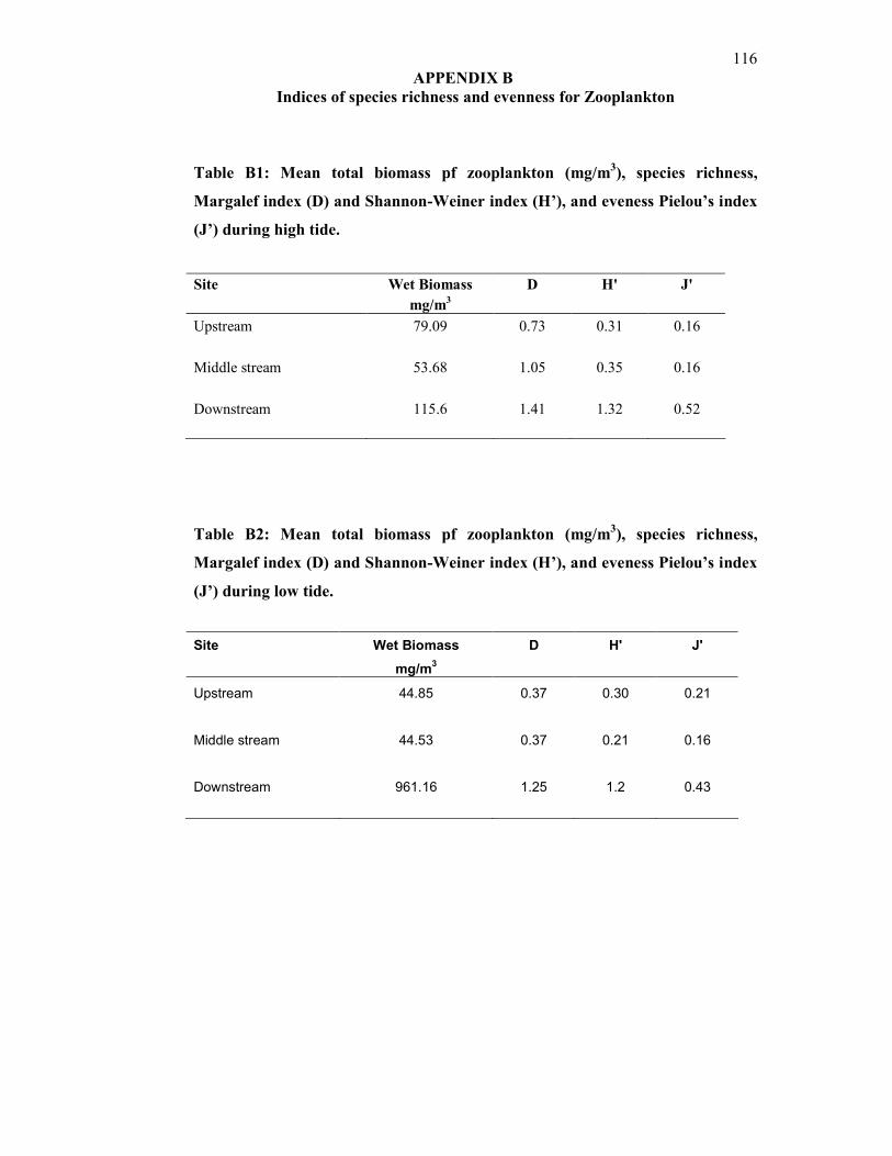
116 APPENDIX B

Indices of species richness and evenness for Zooplankton

Table B1: Mean total biomass pf zooplankton (mg/m3), species richness,

Margalef index (D) and Shannon-Weiner index (H’), and eveness Pielou’s index

(J’) during high tide.

Table B2: Mean total biomass pf zooplankton (mg/m3), species richness,

Margalef index (D) and Shannon-Weiner index (H’), and eveness Pielou’s index

(J’) during low tide.

Site Wet Biomass D H' J'

mg/m3

Upstream 79.09 0.73 0.31 0.16 Middle stream 53.68 1.05 0.35 0.16 Downstream 115.6 1.41 1.32 0.52

Site Wet Biomass D H' J'

mg/m3

Upstream 44.85 0.37 0.30 0.21

Middle stream 44.53 0.37 0.21 0.16

Downstream 961.16 1.25 1.2 0.43

117 APPENDIX C

ANOVA analysis

Table C1: ANOVA analysis between distance and Water Quality Index (WQI)

during high tide with 95 % confident level (P <0.05)

Anova: Two-Factor Without Replication

SUMMARY Count Sum Average Variance Row 1 2 55 27.5 1512.5 Row 2 2 54.5 27.25 1225.125 Row 3 2 54.21 27.105 1141.942 Row 4 2 60.42 30.21 1330.248 Row 5 2 52.26 26.13 789.6338 Row 6 2 59.78 29.89 977.7042 Row 7 2 70.43 35.215 1228.592 Column 1 7 34.6 4.942857 12.26142 Column 2 7 372 53.14286 19.47619 ANOVA

Source of

Variation SS df MS F P-value F crit

Rows 116.02 6 19.33666 1.559289 0.301555 4.283866 Columns 8131.34 1 8131.34 655.703 2.34E-07 5.987378 Error 74.4057 6 12.40095 Total 8321.766 13

Distance from WQI

Station 1

0 55

2.5 52

3.21 51

4.42 56

6.26 46 7.78 52 10.43 60

118 APPENDIX C

ANOVA analysis

Table C2: ANOVA analysis between distance and Water Quality Index (WQI)

during low tide with 95 % confident level (P <0.05)

Anova: Two-Factor Without Replication SUMMARY Count Sum Average Variance

Row 1 2 57 28.5 1624.5 Row 2 2 44.5 22.25 780.125 Row 3 2 50.21 25.105 958.7821 Row 4 2 39.42 19.71 467.5682 Row 5 2 49.26 24.63 674.9138 Row 6 2 56.78 28.39 849.5442 Row 7 2 63.43 31.715 906.1025 Column 1 7 34.6 4.942857 12.26142 Column 2 7 326 46.57143 53.95238 ANOVA

Source of Variation SS df MS F P-value F crit

Rows 201.03 6 33.505 1.024342 0.488728 4.283866 Columns 6065.283 1 6065.283 185.4327 9.74E-06 5.987378 Error 196.2528 6 32.70881 Total 6462.566 13

Distance from WQI

Station 1

0 57

2.5 42

3.21 47

4.42 35

6.26 43

7.78 49

10.43 53

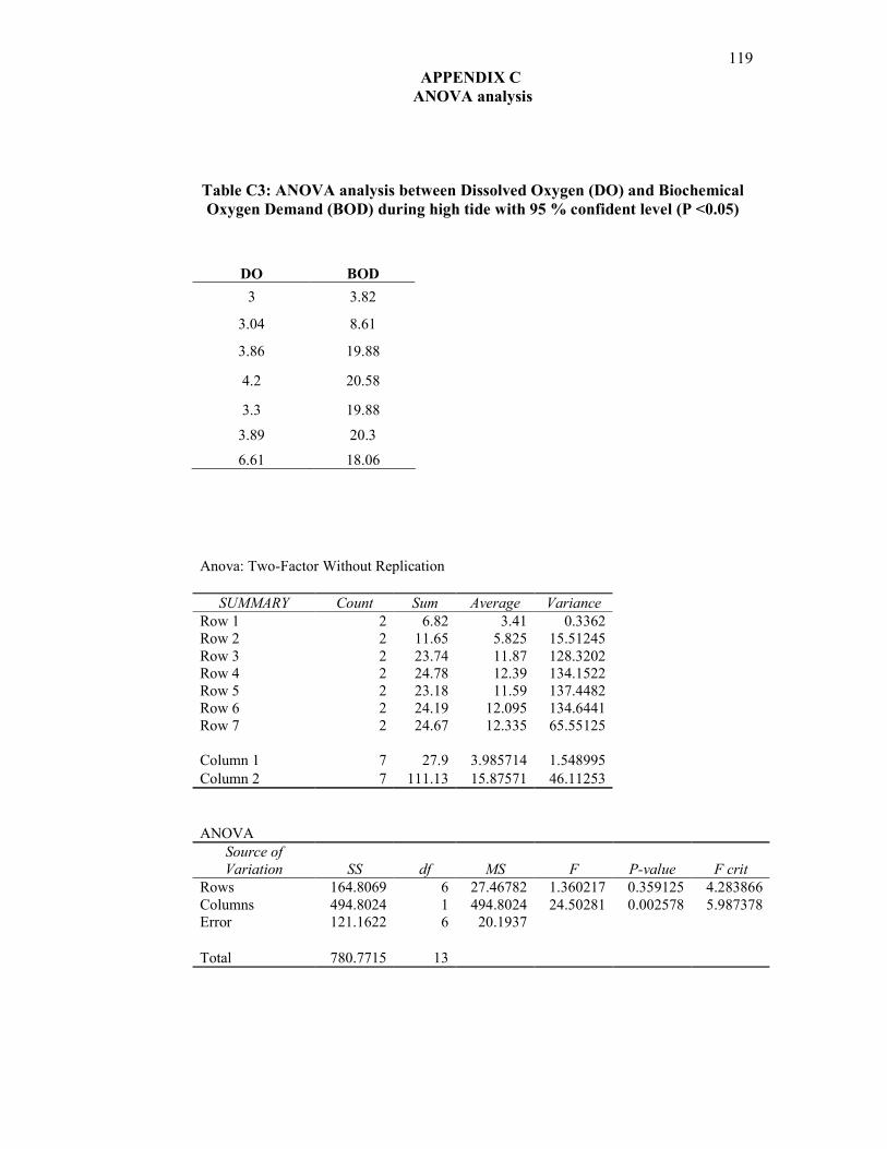
119 APPENDIX C

ANOVA analysis

Table C3: ANOVA analysis between Dissolved Oxygen (DO) and Biochemical

Oxygen Demand (BOD) during high tide with 95 % confident level (P <0.05)

Anova: Two-Factor Without Replication

SUMMARY Count Sum Average Variance Row 1 2 6.82 3.41 0.3362 Row 2 2 11.65 5.825 15.51245 Row 3 2 23.74 11.87 128.3202 Row 4 2 24.78 12.39 134.1522 Row 5 2 23.18 11.59 137.4482 Row 6 2 24.19 12.095 134.6441 Row 7 2 24.67 12.335 65.55125 Column 1 7 27.9 3.985714 1.548995 Column 2 7 111.13 15.87571 46.11253 ANOVA

Source of


Rows 164.8069 6 27.46782 1.360217 0.359125 4.283866 Columns 494.8024 1 494.8024 24.50281 0.002578 5.987378 Error 121.1622 6 20.1937 Total 780.7715 13

DO BOD

3 3.82

3.04 8.61

3.86 19.88

4.2 20.58

3.3 19.88

3.89 20.3

6.61 18.06

120 APPENDIX C

ANOVA analysis

Table C4: ANOVA analysis between Dissolved Oxygen (DO) and Biochemical

Oxygen Demand (BOD) during low tide with 95 % confident level (P <0.05)

Anova: Two-Factor Without Replication SUMMARY Count Sum Average Variance

Row 1 2 8.04 4.02 0.1682 Row 2 2 10.38 5.19 33.9488 Row 3 2 14.39 7.195 67.86125 Row 4 2 23.27 11.635 180.6901 Row 5 2 18.64 9.32 88.1792 Row 6 2 16.54 8.27 79.1282 Row 7 2 25.77 12.885 97.86005 Column 1 7 18.85 2.692857 2.751024 Column 2 7 98.18 14.02571 34.4262 ANOVA

Source of


Rows 124.7453 6 20.79089 1.268795 0.389965 4.283866 Columns 449.5178 1 449.5178 27.43249 0.001943 5.987378 Error 98.31797 6 16.38633 Total 672.5811 13

DO BOD

3.73 4.31

1.07 9.31

1.37 13.02

2.13 21.14

2.68 15.96

1.98 14.56

5.89 19.88

121 APPENDIX D

Times and Height of High Tide and Low Tide water on Sungai Batu Pahat

122 APPENDIX D

Times and Height of High Tide and Low Tide water on Sungai Batu Pahat

123 APPENDIX E

Examples of planktonic life and macroinvertebrates that had been caught

within study area

Figure E1: Biddulphia sp. Figure E2: Codonella sp.

(Bacillariophyceae-phytoplankton) (Bacillariophyceae-phytoplankton)

Figure E3: Ceratium sp. Figure E4: Brachionus sp.

(Dinophyceae-phytoplankton) (Rotifera-zooplankton)

Figure E5: Copepoda sp. Figure E6: Ostracoda sp.

(Crustacea-zooplankton) (Crustacea-zooplankton)

124 APPENDIX E

Examples of planktonic life and macroinvertebrates that had been caught

within study area

Figure E7: Cladoceran sp. Figure E8: Sagitta sp.

(Crustacea-zooplankton) (Chaetognatha -zooplankton)

Figure E9: Nereis sp. Figure E10: Yoldia sp.

(Polycate-Benthos) (Bivalve -benthos)

Figure E11: Nasarius sp.

(Gastropod-Benthos)