A&A 597, A138 (2017)DOI: 10.1051/0004-6361/201527560c© ESO 2017

Astronomy&Astrophysics

Solar Hα features with hot onsets

II. A contrail fibril

R. J. Rutten1, 2 and L. H. M. Rouppe van der Voort2

1 Lingezicht Astrophysics, ’t Oosteneind 9, 4158 CA Deil, The Netherlandse-mail: R.J.Rutten@uu.nl

2 Institute of Theoretical Astrophysics, University of Oslo, PO Box 1029, Blindern, 0315 Oslo, Norway

Received 14 October 2015 / Accepted 22 September 2016

ABSTRACT

The solar chromosphere observed in Hα consists mostly of narrow fibrils. The longest typically originate in network or plage andarch far over adjacent internetwork. We use data from multiple telescopes to analyze one well-observed example in a quiet area. Itresulted from the earlier passage of an accelerating disturbance in which the gas was heated to high temperature as in the spicule-IIphenomenon. After this passage a dark Hα fibril appeared as a contrail. We use Saha-Boltzmann extinction estimation to gauge theonset and subsequent visibilities in various diagnostics and conclude that such Hα fibrils can indeed be contrail phenomena, notindicative of the thermodynamic and magnetic environment when they are observed but of more dynamic happenings before. Theydo not connect across internetwork cells but represent launch tracks of heating events and chart magnetic field during launch, not atpresent.

Key words. Sun: activity – Sun: atmosphere – Sun: magnetic fields

1. Introduction

In the Balmer Hα line at 6563 Å the solar chromosphere showscanopies of long thin features called fibrils. They occur every-where where there is some magnetic activity. Understanding thechromosphere necessitates understanding these. Here we showa case where this requires identifying preceding events and sug-gest that not doing so resembles studying jet contrails in our skywithout appreciating they were made by aircraft.

The literature on Hα fine structure is vast (e.g., the landmarkthesis of Beckers 1964 and the review by Bray & Loughhead1974). We therefore limit our introductory summary to varioustypes of Hα fibrils and only to recent and pertinent results.

The first type are dynamic fibrils. The name was given byHansteen et al. (2006) and De Pontieu et al. (2007a) who afterdecades of slack progress since Beckers’ thesis identified andexplained a particular Hα fibril type. These are fairly short darkfibrils that jut out in phased rows from plage and active net-work, representing field-guided acoustic shock waves sloshed upby the p-mode interference pattern into relatively tenuous mag-netic field bundles. Short dynamic fibrils are similar but occurin sunspot chromospheres (Rouppe van der Voort & de la CruzRodríguez 2013; Yurchyshyn et al. 2014).

The second type of fibrils are spicules-II discovered byDe Pontieu et al. (2007b). They are long, slender, highly dy-namic jets jutting out from the limb, with much dynamics at-tributed to multiple Alfvénic wave modes (e.g., De Pontieu et al.2007c, 2012; McIntosh et al. 2008). Their manifestations onthe disk are slender jet-like Doppler-shifted features observedin the wings of Hα and Ca ii 8542 Å as rapid blueshifted excur-sions (RBE) and rapid redshifted excursions (RRE) (Langangenet al. 2008; Rouppe van der Voort et al. 2009; Sekse et al. 2012,2013). Their tops get very hot (De Pontieu et al. 2011; Pereiraet al. 2014; Rouppe van der Voort et al. 2015; Skogsrud et al.2015). They tend to arise from plage and active network in

areas that are not too active and mainly unipolar (e.g., Fig. 2of Rouppe van der Voort et al. 2009) and favor quiet Sun andcoronal holes (Pereira et al. 2012).

Finally, there are long fibrils. With this name we denote theubiquitous slender Hα structures that jut out from network andplage and reach far out over adjacent internetwork, often givingthe impression of spanning from one side of a supergranulationcell to another tracing closed-field canopies. We suggest belowthat this interpretation is not correct and therefore do not wantto call them “long closed-loop fibrils”, nor “long internetworkfibrils” because they invariably are rooted in network or plageat least on one side. We thought about “long arching fibrils” be-cause they are generally curved, more so than dynamic fibrils,but eventually chose to simply call them long fibrils.

They are absent only in the very quietest areas(Rouppe van der Voort et al. 2007), but prominently coverthe solar surface above active regions and widely around them.Overall they constitute the chromosphere as named by Lockyer(1868). Their nature remains unclear, nor whether they actuallymap magnetic fields as one naturally supposes when viewingtheir patterns. They are often interpreted as cylindrical fluxtubes (e.g., Foukal 1971; Sánchez-Andrade Nuño et al. 2008),but also as sheets or warps in sheets (Judge et al. 2011; Lipartitoet al. 2014) or as density corrugations (Leenaarts et al. 2012,2015).

Here we detail the formation of a single long Hα fib-ril which we deem potentially exemplary for the class. Ourstudy was triggered by a study of Ellerman bomb visibilities(Rutten 2016, henceforth Pub 1) which was inspired by the 2Dnon-equilibrium MHD simulation of Leenaarts et al. (2007)called HION henceforth following Pub 1. The effects of dynamichydrogen ionization in the HION atmosphere defined the fol-lowing recipe to understand marked presence of Hα in and af-ter dynamical instances with hot and dense onsets: (1) evaluate

Article published by EDP Sciences A138, page 1 of 10

A&A 597, A138 (2017)

0

10

20

30

40

50

y [a

rcse

c]

Fe I wide band

0

10

20

30

40

50Fe I magnetogram

0

10

20

30

40

50Ca II 8542 blue wing

0

10

20

30

40

50Hα line center

0 10 20 30 40 50x [arcsec]

0

10

20

30

40

50

y [a

rcse

c]

SJI 1400 Å

0 10 20 30 40 50x [arcsec]

0

10

20

30

40

50He II 304 Å

0 10 20 30 40 50x [arcsec]

0

10

20

30

40

50Fe IX 171 Å

0 10 20 30 40 50x [arcsec]

0

10

20

30

40

50Fe XII 193 Å

Fig. 1. Overview of the observed area at 08:22:23 UT. The field of view was centered at solar (X,Y) = (−202, 206) arcsec with viewing angleµ = 0.95. It is clockwise rotated with respect to (X,Y) over 62.6◦. The arrow in the second panel points to disk center. Upper row: SST images:Fe i 6303 Å wide band, Fe i 6303 Å magnetogram, blue wing of Ca ii 8542 Å at ∆λ = −0.7 Å from line center, Hα line center. Lower row: corre-sponding images from IRIS and SDO/AIA: 1400 Å slitjaw, He ii 304, Å Fe ix 171 Å, Fexii 193 Å. The pixel sizes are 0.057 arcsec for the SST,0.167 arcsec for IRIS, 0.6 arcsec for AIA. The white frame defines the subfield used in Fig. 2. In the fourth panel it contains the long black archingfibril discussed here.

the Hα extinction coefficient (H i n = 2 level population) duringthe onset by assuming the Saha-Boltzmann (SB) value; (2) usethe resulting large population also for cooler surrounding gasin reach of scattering Lyα radiation from the hot structure; and(3) maintain this large population subsequently during coolingand recombination.

This post-Saha-Boltzmann-extinction (PSBE) recipe holdsfor shocks in the HION atmosphere and was applied successfullyto Ellerman bombs in Pub 1, including the suggestion that it ap-plies partially even to the Si iv lines observed with the InterfaceRegion Imaging Spectrograph (IRIS, De Pontieu et al. 2014)which commonly are interpreted assuming coronal equilibrium(CE). This condition is the opposite of SB equilibrium by requir-ing statistical equilibrium in which collisional deexcitation andrecombination are fully negligible instead of fully dominating.

A corollary of Pub 1 is that other Hα features with hot anddense onsets may similarly gain large SB extinction at such mo-ments and then retain these high values during subsequent cool-ing. Reversely, features with unusual opaqueness in Hαmay rep-resent products of hot and dense onset phenomena. Since longfibrils represent a class of Hα features with intriguing opac-ities, we wondered whether preceding hot instances might befound producing them. The question became how to identifysuch precursors.

A 2014 multi-telescope campaign utilizing “last photons” ofthe SUMER spectrometer (Wilhelm et al. 1995) was undertakento search for hot precursors in Lyman lines, but without suc-cess. We then found a striking example in high-resolution Hαimaging spectroscopy from the Swedish 1-m Solar Telescope(SST, Scharmer et al. 2003) together with hotter diagnosticsfrom the Atmospheric Imaging Assembly (AIA, Lemen et al.2012) onboard the Solar Dynamics Observatory (SDO, Pesnellet al. 2012), and saw it confirmed in sharper images from IRIS.

Here we present and discuss this example, which we call “con-trail fibril”.

The observations are detailed in the next section. The dis-plays combine extracts of the multiple data sets that, whenviewed and blinked as multi-diagnostic movies, led to our notic-ing the feature. In Sect. 3 we estimate the visibilities of its onset,contrail, and aftermath. In the discussion (Sect. 4) we argue thatthe phenomenon shared characteristics with spicules-II and spec-ulate about why such features become so long, what they tell usabout magnetic field topography, and how ubiquitous they are.We conclude the study and outline follow-up in Sect. 5.

2. Observations

2.1. Data collection and reduction

For this study we analyzed data from a joint SST−IRIS ob-serving campaign targeting a quiet area near solar disk center.Figure 1 gives an overview.

On June 21, 2014 the second author obtained imaging spec-troscopy at the SST with the CRisp Imaging SpectroPolarimeter(CRISP, Scharmer et al. 2008) during 08:02−09:15 UT ata cadence of 11.5 s. Hα was sampled at 15 wavelengthsspanning ±1.4 Å from line center, Ca ii 8542 Å at 25 wave-lengths spanning ±1.2 Å from line center, Stokes-V magne-tograms were obtained in Fe i 6303 Å. The reduction used theCRISPRED pipeline of de la Cruz Rodríguez et al. (2015).It included dark and flat field correction, multi-object multi-frame blind deconvolution (van Noort et al. 2005), minimizationof remaining small-scale deformation through cross-correlation(Henriques 2012), prefilter transmission correction followingde la Cruz Rodriguéz (2010), correction for time-dependent im-age rotation due to the alt-azimuth telescope configuration, and

A138, page 2 of 10

R. J. Rutten and L. H. M. Rouppe van der Voort: Solar Hα features with hot onsets. II

0

5

10

15

y [a

rcse

c]

Hα −0.8 Å

1 08:14:18

1

0

5

10

15Hα center

1

0

5

10

15SJI 1400 Å

1

0

5

10

15He II 304 Å

1

0

5

10

15Fe XII 193 Å

1

0

5

10

15

y [a

rcse

c]

H −0.8 Å

2 08:16:24

1 2

0

5

10

15H center

1 2

0

5

10

15SJI 1400 Å

1 2

0

5

10

15He II 304 Å

1 2

0

5

10

15Fe XII 193 Å

1 2

0

5

10

15

y [a

rcse

c]

H −0.8 Å

3 08:18:10

1 2 3

0

5

10

15H center

1 2 3

0

5

10

15SJI 1400 Å

1 2 3

0

5

10

15He II 304 Å

1 2 3

0

5

10

15Fe XII 193 Å

1 2 3

0

5

10

15

y [a

rcse

c]

H −0.8 Å

4 08:19:42

1 2 3

4

0

5

10

15H center

1 2 3

4

0

5

10

15SJI 1400 Å

1 2 3

4

0

5

10

15He II 304 Å

1 2 3

4

0

5

10

15Fe XII 193 Å

1 2 3

4

0

5

10

15

y [a

rcse

c]

H −0.8 Å

5 08:20:51

1 2 3

4

0

5

10

15H center

1 2 3

4

0

5

10

15SJI 1400 Å

1 2 3

4

0

5

10

15He II 304 Å

1 2 3

4

0

5

10

15Fe XII 193 Å

1 2 3

4

0

5

10

15

y [a

rcse

c]

H −0.8 Å

6 08:22:23

1 2 3

4

0

5

10

15H center

1 2 3

4

0

5

10

15SJI 1400 Å

1 2 3

4

0

5

10

15He II 304 Å

1 2 3

4

0

5

10

15Fe XII 193 Å

1 2 3

4

0

5

10

15

y [a

rcse

c]

H −0.8 Å

7 08:23:55

1 2 3

4

0

5

10

15H center

1 2 3

4

0

5

10

15SJI 1400 Å

1 2 3

4

0

5

10

15He II 304 Å

1 2 3

4

0

5

10

15Fe XII 193 Å

1 2 3

4

0

5

10

15

y [a

rcse

c]

H −0.8 Å

8 08:25:03

1 2 3

4

0

5

10

15H center

1 2 3

4

0

5

10

15SJI 1400 Å

1 2 3

4

0

5

10

15He II 304 Å

1 2 3

4

0

5

10

15Fe XII 193 Å

1 2 3

4

0 5 10 15 20x [arcsec]

0

5

10

15

y [a

rcse

c]

H −0.8 Å

9 08:27:33

1 2 3

4

0 5 10 15 20x [arcsec]

0

5

10

15H center

1 2 3

4

0 5 10 15 20x [arcsec]

0

5

10

15SJI 1400 Å

1 2 3

4

0 5 10 15 20x [arcsec]

0

5

10

15He II 304 Å

1 2 3

4

0 5 10 15 20x [arcsec]

0

5

10

15Fe XII 193 Å

1 2 3

4

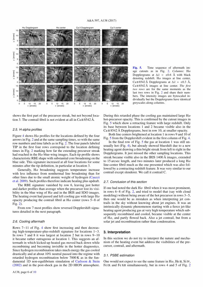
Fig. 2. Time sequence of image cutouts defined by the subfield frame in Fig. 1. The row number and the observing moment of each row arespecified in the first panel of each row. Columns: Hα images at ∆λ=−0.8 Å from line center (SST), Hα line center (SST), 1400 Å slitjaw (IRIS),He ii 304 Å (AIA), Fexii 193 Å (AIA). The four numbered arrows mark the location of the tip of the dark extending precursor streak definedsuccessively for the first four Hα blue-wing panels. Each frame is bytescaled individually. Row 6 corresponds to Fig. 1. The IRIS slit is visible inthe top two and bottom two 1400 Å panels.

A138, page 3 of 10

A&A 597, A138 (2017)

0

5

10

15

y [a

rcse

c]

Hα −0.8 Å

4 08:19:42

1 2 3

4

0

5

10

15

Hα center

1 2 3

4

0

5

10

15

Ca II −0.7 Å

1 2 3

4

0

5

10

15

Ca II center

1 2 3

4

0

5

10

15

Fe IX 171 Å

1 2 3

4

0 5 10 15 20x [arcsec]

0

5

10

15

y [a

rcse

c]

H −0.8 Å

6 08:22:23

1 2 3

4

0 5 10 15 20x [arcsec]

0

5

10

15

H center

1 2 3

4

0 5 10 15 20x [arcsec]

0

5

10

15

Ca II −0.7 Å

1 2 3

4

0 5 10 15 20x [arcsec]

0

5

10

15

Ca II center

1 2 3

4

0 5 10 15 20x [arcsec]

0

5

10

15

Fe IX 171 Å

1 2 3

4

Fig. 3. Image cutouts as in Fig. 2. The first two columns repeat the first panels of rows 4 and 6 in Fig. 2. The third and fourth columns containcorresponding cutouts of Ca ii 8542 Å, in the blue wing at ∆λ =−0.7 Å from line center and at line center. The last column contains correspondingcutouts from Fe ix 171 Å (AIA).

removal of remaining rubber-sheet distortions by destretching(Shine et al. 1994).

The same region was observed with IRIS. Unfortunately, itsscanning spectrograph slit missed the feature described here sothat we only use slitjaw images in the 1400 Å passband. Theseare dominated by the Si iv doublet at 1394 Å and 1403 Å in high-temperature gas (e.g., Vissers et al. 2015).

In addition, we collected corresponding image sequencesfrom SDO. All image sequences were rotated to the SST im-age orientation and precisely co-aligned using interpolation ofthe space-based images to the spatial and temporal grid of theSST images. This was done with the SolarSoft library and IDLprograms available on the website of the first author.

The PSBE recipe defined in Pub 1 led us to search for fea-tures with large Hα extinction that follow on hot-onset precur-sors. While inspecting the SST and AIA diagnostics using theCRisp SPectral EXplorer (CRISPEX; Vissers & Rouppe van derVoort 2012) as browser to compare and blink time-delay movies,we quickly noted that the prominent dark Hα fibril in Fig. 1was preceded minutes earlier by a fast-moving bright blob inHe ii 304 Å and that the Hα fibril outlined the passage of thisdisturbance. Subsequently, we found that the latter was mappedvery well in the outer blue wing of Hα. When we then co-aligned the 1400 Å slitjaw images from IRIS we found bright-ening that clearly tracks the same disturbance. Figs. 1−3 presentthe phenomenon.

2.2. Field of view

Figure 1 shows the observed region. It was very quiet, far fromAR 12093 and AR 12094 on the southern hemisphere. The firstpanel shows that it contained only a small pore besides granu-lation and tiny magnetic network concentrations in intergranularlanes. At the SST resolution the latter appear as bright pointseven in the continuum (we invite the reader to zoom in per pdfviewer). The magnetogram in the second panel shows that thesetogether constituted fairly dense patches of active network. Theother diagnostics show corresponding brightness features.

The blue wing of Ca ii 8542 Å (third panel) maps magneticconcentrations as enhanced brightness and elsewhere displaysreverse granulation in the mid photosphere (Rutten et al. 2011).The Hα core samples the fibrilar chromosphere. In this quietfield long fibrils extend from the network patches but are less

ubiquitous elsewhere. Some seem to connect the main opposite-polarity patches across the center of the field, but our feature,the large black fibril within the overlaid frame, does not reachthat far. Elsewhere, notably in the lower-left corner, the Hα im-age shows non-fibrilar swirly brightness patterns which probablyrepresent acoustic shock patterns (Rutten et al. 2008).

The diagnostics in the lower row show increasingly diffusebrightness response to the enhanced network areas. The 1400 Åpanel shows largest brightness near the polarity reversal betweenthe main field concentrations, possibly from earlier reconnec-tion, and elsewhere bright points as the ones ascribed to acousticshocks by Martínez-Sykora et al. (2015).

The three AIA panels show a larger brightness blob abovethe network patches indicating heating of the higher atmosphere.There are similarities, even in fine structure, between He ii 304and Fe ii 193 Å and more diffuse veiling originating further tothe left that seems to cover this fine structure in Fe ii 193 Å andyet more in Fe ix 171 Å.

2.3. Precursor and contrail

Figure 2 details the dark Hα line-center fibril that we call the“contrail fibril” and is the topic of this study. It is prominent inthe second column in rows 5−8, longest in row 6. It is muchweaker or absent in the preceding rows, but the blue-wing im-ages in the first column show a long, slender, growing dark fea-ture at the same location with bright counterparts in the IRIS andAIA columns.

The action started with a fan of RBE extensions near the footof the contrail fibril. It first shot off a long RBE towards the upperleft, sampled in the first panel of Fig. 2. Unfortunately, the IRISslit had just passed (dark slanted line in the top 1400 Å panel).

Subsequently, the dark extensions seen in the secondHα-wing panel (we again invite the reader to zoom in per pdfviewer) fanned out progressively in shooting off growing RBEsfrom left to right as in a peacock tail display, finally sending offthe long precursor of our contrail fibril towards the right. Thelatter’s extension progress is marked by the four arrows. Eachwas placed successively at the tip of the growing dark blue-wingfeature in rows 1−4. The Hα profiles in Fig. 4 are for these fourlocations.

The second arrow actually identifies the tip of another RBEshot off in parallel to the main one pointed at later by arrows 3and 4. This was also a precursor: it later produced its own,

A138, page 4 of 10

R. J. Rutten and L. H. M. Rouppe van der Voort: Solar Hα features with hot onsets. II

0

20

40

60

80

inte

nsity

−50 0 50∆λ [km s−1]

1 08:14:18

TIP 1

0

20

40

60

80−50 0 50

∆λ [km s−1]

0

20

40

60

80−50 0 50

∆λ [km s−1]

0

20

40

60

80−50 0 50

∆λ [km s−1]

0

20

40

60

80

inte

nsity

−50 0 50

2 08:16:240

20

40

60

80−50 0 50

TIP 2

0

20

40

60

80−50 0 50

0

20

40

60

80−50 0 50

0

20

40

60

80

inte

nsity

−50 0 50

3 08:18:100

20

40

60

80−50 0 50

0

20

40

60

80−50 0 50

TIP 3

0

20

40

60

80−50 0 50

0

20

40

60

80

inte

nsity

−50 0 50

4 08:19:420

20

40

60

80−50 0 50

0

20

40

60

80−50 0 50

0

20

40

60

80−50 0 50

TIP 4

0

20

40

60

80

inte

nsity

−50 0 50

5 08:20:510

20

40

60

80−50 0 50

0

20

40

60

80−50 0 50

0

20

40

60

80−50 0 50

0

20

40

60

80

inte

nsity

−50 0 50

6 08:22:230

20

40

60

80−50 0 50

0

20

40

60

80−50 0 50

0

20

40

60

80−50 0 50

0

20

40

60

80

inte

nsity

−50 0 50

7 08:23:550

20

40

60

80−50 0 50

0

20

40

60

80−50 0 50

0

20

40

60

80−50 0 50

0

20

40

60

80

inte

nsity

−50 0 50

8 08:25:030

20

40

60

80−50 0 50

0

20

40

60

80−50 0 50

0

20

40

60

80−50 0 50

0

20

40

60

80

inte

nsity

−50 0 50

9 08:27:330

20

40

60

80−50 0 50

0

20

40

60

80−50 0 50

0

20

40

60

80−50 0 50

0

20

40

60

80

inte

nsity

−50 0 50

10 08:29:510

20

40

60

80−50 0 50

0

20

40

60

80−50 0 50

0

20

40

60

80−50 0 50

−1 0 1∆ λ [Å]

0

20

40

60

80

inte

nsity

−50 0 50

11 08:31:57

−1 0 1∆ λ [Å]

0

20

40

60

80−50 0 50

−1 0 1∆ λ [Å]

0

20

40

60

80−50 0 50

−1 0 1∆ λ [Å]

0

20

40

60

80−50 0 50

Fig. 4. Hα profiles at the four locations marked by arrows in Fig. 2. Thewavelength separation from line center is given in Å at the bottom, inkm s−1 at the top. The intensity scale is arbitrary. The first nine rows arethe same time samplings and have the same numbers as in Fig. 2, sim-ilarly specified in the first column. The last four rows are for the sametimes as in Fig. 5. The columns correspond to the initial precursor-tiplocations marked by the four arrows in Fig. 2. The panels for their defin-ing moment are labeled “TIP” in the first four rows. Solid: Hα profile atthis location and time. Dashed: mean profile of the whole sequence forreference, identical in all panels. Dotted, vertical: sampling wavelengthsused in Fig. 2.

shorter, and more curved contrail (dark fibril in Hα line center inrows 4−6). We call this contrail B.

The mean proper motion speeds over the surface defined bythe arrow-marked tip locations of the main dark streak in the ini-tial blue-wing images in the first column of Fig. 2 are 13, 15,and 53 km s−1 for 1→2, 2→3, and 3→4, respectively. It acceler-ated appreciably. The last value is similar to the speeds reachedby RBEs (Rouppe van der Voort et al. 2009), but this streak wasmuch longer when it reached 15-arcsec extension five minutesafter its launch (row 4; observing times are specified in the firstcolumn).

The dark fibril at the center of Hα appeared a minute laterand lasted four minutes (second column, rows 5−8). It faith-fully mapped the precursor shape and therefore represents a post-passage contrail.

Actually, we first noted the extending precursor in theHe ii 304 Å sequence (fourth column) where it is most clearlyevident in rows 3−6. We then recognized its presence (when youknow what to look for) also in the Fe ix 171 Å and Fexii 193 Åimages. We sample only the latter in Fig. 2 in order not to makeits panels too small, but Fig. 3 shows the corresponding Fe ix171 Å cutouts at the times of rows 4 and 6 of Fig. 2.

Only afterwards we noted the slender precursor in the Hαwing images and realized from inspecting the Hα profiles withCRISPEX that it is so dark from RBE signature including largeline broadening. This is detailed with profile samples in Fig. 4.

Later we co-aligned the IRIS images and found that the pre-cursor is very evident in the 1400 Å slitjaw images (third columnof Fig. 2). In rows 3−5 it appears as a very thin extending streakstarting at location 3 and extending to but not reaching loca-tion 4. An underlying bright point, also present before and after,was enhanced by the streak which implies optically thin forma-tion of the Si iv lines in the streak and therefore direct imaging ofintrinsic fine structure, in particular the narrow precursor width.

Figure 2 shows that the precursor became hotter alongits track. The 1400 Å and hotter diagnostics do not show itsstart from location 1 to location 3 in rows 1−3, only the partfrom 3 to 4 in rows 4−6, but in 1400 Å the streak does notreach location 4. In He ii 304 Å and Fexii 193 Å the streakis most evident closer to location 4 (row 4), and well-evidentin Fe ix 171 Å between these locations (Fig. 3). This suggestsincreasing ionization along the track to very high degree, withSi iv peaking closer to location 3 and the highest iron stage clos-est to location 4.

In summary, a sudden event in the low atmosphere sentoff a disturbance that heated gas along its path to very hightemperature.

By row 6, seven minutes after its onset, the precursor becameinvisible, but by then had left the black fibril at Hα line centeralong its wake. This contrail persisted three more minutes.

By 08:27 UT (row 9) the show was over in these high-temperature diagnostics − just when the IRIS slit was nearingin the next scan (bottom 1400 Å panel). It is a pity that the scantiming missed the Si iv emission streak in rows 4−6 because theslit happened to be aligned with its direction.

2.4. Comparison with Ca II 8542 Å

Figure 3 adds cutout images in Ca ii 8542 Å and Fe ix 171 Åfor key moments in Fig. 2: the time when the precursor streakreached its maximum length in the blue wing of Hα (row 4) andnearly three minutes later (row 6) when the line-center contrailfibril reached maximum visibility. The Ca ii 8542 Å wing image

A138, page 5 of 10

A&A 597, A138 (2017)

0

5

10

15

y

[arc

se

c]

Hα Dopplergram

8 08:25:03

1 2 3

4

0

5

10

15

Hα center

1 2 3

4

0

5

10

15

Ca II Dopplergram

1 2 3

4

0

5

10

15

Ca II center

1 2 3

4

0

5

10

15

y [a

rcsec]

H Dopplergram

9 08:27:33

1 2 3

4

0

5

10

15

H center

1 2 3

4

0

5

10

15

Ca II Dopplergram

1 2 3

4

0

5

10

15

Ca II center

1 2 3

4

0

5

10

15

y [a

rcsec]

H Dopplergram

10 08:29:51

1 2 3

4

0

5

10

15

H center

1 2 3

4

0

5

10

15

Ca II Dopplergram

1 2 3

4

0

5

10

15

Ca II center

1 2 3

4

0 5 10 15 20x [arcsec]

0

5

10

15

y

[arc

se

c]

H Dopplergram

11 08:31:57

1 2 3

4

0 5 10 15 20x [arcsec]

0

5

10

15

H center

1 2 3

4

0 5 10 15 20x [arcsec]

0

5

10

15

Ca II Dopplergram

1 2 3

4

0 5 10 15 20x [arcsec]

0

5

10

15

Ca II center

1 2 3

4

Fig. 5. Time sequence of aftermath im-age cutouts as in Fig. 2. Columns: HαDopplergrams at ∆λ = ±0.6 Å with blackdenoting redshift. Hα images at line center,Ca ii 8542 Å Dopplergrams at ∆λ = ±0.3 Å,Ca ii 8542 Å images at line center. The firsttwo rows are for the same moments as thelast two rows in Fig. 2 and share their num-bers. The intensity images are bytescaled in-dividually but the Dopplergrams have identicalgreyscales along columns.

shows the first part of the precursor streak, but not beyond loca-tion 3. The contrail fibril is not evident at all in Ca ii 8542 Å.

2.5. H-alpha profiles

Figure 4 shows Hα profiles for the locations defined by the fourarrows in Fig. 2 and at the same sampling times, so with the samerow numbers and time labels as in Fig. 2. The four panels labeledTIP in the first four rows correspond to the location definingtimes in Fig. 2 marking how far the extending precursor streakhad reached in the Hα blue-wing images. Each tip profile showscharacteristic RBE shape with substantial core broadening on theblue side. This signature increased at all four locations for someminutes after the tip definition, in particular at location 3.

Generally, Hα broadening suggests temperature increasewith less influence from nonthermal line broadening than forother lines due to the small atomic weight of hydrogen (Cauzziet al. 2009). Such profiles therefore indicate heating plus updraft.

The RBE signature vanished by row 6, leaving just hotterand darker profiles than average when the precursor lost its visi-bility in the blue wing of Hα and in the IRIS and SDO images.The heating event had passed and left cooling gas with large Hαopacity producing the contrail fibril at Hα center (rows 5−8 ofFig. 2).

From row 7 most profiles show reversed Dopplershift signa-tures detailed in the next paragraph.

2.6. Cooling aftermath

Rows 7−11 of Fig. 4 show first increasing and then decreas-ing high-temperature-plus-redshift signature for locations 1−3.In rows 7 and 8 it was largest at location 2 but in rows 9−10it became rather outrageous at location 1. This suggests an af-termath in which kicked-up heated gas moved back down whilerecombining and becoming invisible in the hotter diagnostics.Since hydrogen recombination takes much energy the gas cooleddrastically and at about 10% neutral passed into the regime withretarded hydrogen recombination below 7000 K as in the fun-damental 1D non-equilibrium simulation of Carlsson & Stein(2002) and in the post-shock gas in the 2D HION atmosphere.

During this retarded phase the cooling gas maintained large Hαhot-precursor opacity. This is confirmed by the cutout images inFig. 5 which show a retracting feature with large redshift. Onlyits base between locations 1 and 2 became visible also in theCa ii 8542 Å Dopplergrams, best in row 10, at smaller opacity.

Both line centers brightened at location 1 in rows 9 and 10 ofFig. 5 from the Dopplershift evident in the first column of Fig. 4.

In the final row of Fig. 5 the gas at location 1 was still un-usually hot (Fig. 4), but already showed blueshift due to a newheating agent drawing a thin bright streak from left to right in theDopplergrams. It just missed the other sampling locations. Thisstreak became visible also in the IRIS 1400 Å images, extendedto 15 arcsec length, and two minutes later produced a long Hαline-center fibril much as the one presented which was also fol-lowed by a contracting redshift feature. It was very similar to ourcontrail except slenderer. We call it contrail C.

2.7. Conclusion of this section

If one had noted the dark Hα fibril when it was most prominent,in rows 6−8 of Fig. 2, and tried to model that (say with cloudmodeling) without being aware of the hot precursor in rows 3−5,then one would be as mistaken as when interpreting jet con-trails in the sky without knowing about jet engines. It was anintrinsically dynamic phenomenon starting with a fierce jet-likeheating agent producing gas at very high temperature which sub-sequently recombined and cooled, became visible at the centerof Hα, and partly flowed back. Also a jet contrail, but from asolar jet and recombination rather than condensation.

3. Interpretation

In this section we do not try to interpret the nature and mecha-nism of the heating event but address the visibilities of the pre-cursor, contrail, and aftermath.

3.1. PSBE estimation

One would not expect to see the same feature in Hα, He ii, Si iv,Fe ix and Fexii simultaneously, but in rows 4 and 5 of Fig. 2

A138, page 6 of 10

R. J. Rutten and L. H. M. Rouppe van der Voort: Solar Hα features with hot onsets. II

10-6

10-4

10-2

100

fraction

IH CE

II

10-6

10-4

10-2

100

fraction

H SB

II

0.0

0.5

1.0

fraction

IHe CE

II III

0.0

0.5

1.0

fraction

He SB

II III

0.0

0.5

1.0

fraction

I

Si CEII III

IV

V

VI VIIVIIIIX X

XIXII

0.0

0.5

1.0

fraction

Si SB

II III IV V VIVIIVIIIIXXXIXII

XIII

XIV

0.0

0.5

1.0

fraction

I

Fe CEII III IVV VI

VII

VIII

IX

X XIXIIXIIIXIVXV

4.0 4.5 5.0 5.5 6.0log (temperature) [K]

0.0

0.5

1.0

fra

ctio

n

Fe SB

II III IV V VIVIIVIIIIXXXIXII

XIIIXIVXVXVI

XVII

XVIIIXIXXXXXI XXIIXXIIIXXIV

XXV

Fig. 6. CE/SB ionization-stage population comparisons for H, He, Siand Fe. Upper panel of each pair: CE distribution with temperature.Lower panel of each pair: SB distribution with temperature for fixedelectron density Ne = 1014 cm−3. For lower Ne the SB curve patternsremain similar but the flanks steepen and the peaks shift leftward (about−0.05 in log(T ) for tenfold Ne reduction). The first pair for hydrogenhas logarithmic y-axes; the dashed curves are on the linear scales of theother panels.

the onset streaks correspond fairly closely between these diag-nostics. Obviously, they are due to some process causing largeheating (Sect. 4). It was initiated along the row of dark exten-sions in the Hα blue-wing image in row 2 of Fig. 2 in the lowatmosphere, implying dense gas for the onset. The combinationof hot and dense makes the PSBE recipe of Pub 1 appropriate forexplaining the joint precursor visibilities in these very disparatediagnostics and the subsequent appearance of the Hα line-centercontrail and its aftermath.

The recipe employs Figs. 6 and 7. They resemble Figs. 4and 5 of Pub 1 and were made as described there. Figure 6 com-pares CE ionization distributions with their SB counterparts over

−15

−10

−5

0

log (

extinction)

[c

m−

1]

Hα

Ca II

He II

Si IV Fe IXFe XII

NH = 1014

15

20

25

log (

density)

[c

m−

3]

NHI Ne

3.5 4.0 4.5 5.0 5.5log (temperature) [K]

−15

−10

−5

log (

extinction)

[c

m−

1]

HαCa II

He II

Si IV Fe IXFe XII

NH = 1012

10

15

20

25

log (

density)

[c

m−

3]

NHI Ne

Fig. 7. SB extinction αl for Hα (solid), Ca ii 8542 Å (solid), He ii 304 Å(dashed), Si iv 1394 Å (dot-dashed), Fe ix 171 Å (dot-dashed) andFexii 193 Å (dotted) as function of temperature, for total hydrogen den-sities NH = 1014 and 1012 cm−3 (upper and lower panel, respectively).The two cross-over solid curves near the bottom are the competing neu-tral hydrogen and electron density, with scales on the right. The extinc-tion scales at left and the density scales at right shift upward betweenthe panels to compensate for the density decrease. The horizontal lineat logαl = −7 marks optical thickness unity for a slab of 100 km geo-metrical thickness.

a wide temperature range. Figure 7 quantifies SB extinction coef-ficients for the specified lines as function of temperature, for totalhydrogen densities corresponding to heights 850 and 1520 kmin the chromosphere of the ALC7 standard model of Avrett &Loeser (2008).

Figure 6 quantifies the large differences in the temperaturesat which successive ionization stages of the plotted elementsreach maximum presence between the SB and CE extremes. Forexample, the IRIS Si iv lines typically form at 80 000 K in CEbut at 16 000 K when SB holds. Such pair comparison definesthe range from SB validity at very high density to CE validity atvery low density.

SB extinction can be valid in momentary hot and denseinstances at chromospheric heights where generally NLTE isthe rule. When the gas becomes so hot that hydrogen ionizessubstantially, the resulting large boost of the electron densitymay create collisionally constrained SB populations at suffi-ciently high gas density and feature thickness. This then holdsusually only for lower levels of resonance lines, not for their up-per levels because these suffer NLTE photon losses.

Hα is a special case because it rides on top of Lyα in whicheven a small neutral-hydrogen feature can be sufficiently opaqueto thermalize Lyα radiation notwithstanding the very small Lyαcollision rates. This is the case throughout the ALC7 chromo-sphere (Fig. 1 of Pub 1) and also within the HION shocks. In thelatter the Hα extinction reaches the SB value at electron densitiesas low as 109 cm−3 thanks to 10% hydrogen ionization produc-ing 103 more electrons than available from the electron-donormetals in cooler gas (Fig. 2 of Leenaarts et al. 2007).

A138, page 7 of 10

A&A 597, A138 (2017)

SB extinction is also a good assumption for Ca ii 8542 Å(Pub 1) and applies to resonance lines of majority species wher-ever the Saha law applies, which at high density is more likelythan CE. Therefore, the curves for Hα and Ca ii 8542 Å in Fig. 7are probably correct where they peak, whereas the temperaturelocations of the peaks for the higher ions represent lower limitsonly. However, even for these peaks shifts as far to the right aspredicted by CE (Fig. 6) are unlikely.

3.2. Precursor visibilities

The Hα curves in Fig. 7 are for line center. For the Hα wingvisibility they should be shifted down over about one logarith-mic unit and so get significantly below the horizontal line in thelower panel. The choice of a 100-km slab as geometrical fea-ture thickness is arbitrary. The width of the blue-wing precursorin the first column of Fig. 2 measures about 1 arcsec or 700 kmbut this is widened by resonance scattering in Lyα (Pub 1). Theintrinsic precursor width shown by the 1400 Å panels is sub-arcsecond. The 100-km line should therefore be a reasonablevisibility indicator.

Because the Hα curves drop less steeply then the others Hαmay still reach overlap visibility with He ii and Si iv as predictedin the upper panel of Fig. 6 and observed in the first, third andfourth panels of row 4 of Fig. 2 (remember that both extinctionand emissivity scale with the lower-level population). Since theinitial part of the Hα-wing precursor is not visible in these hotterdiagnostics it started well below 15 000 K but then became muchhotter.

The Ca ii 8542 Å visibility constrains the initial temperatureof the precursor to yet lower values. The curves for this lineand for Hα in Fig. 7 cross at T ≈ 6000 K with nearly oppo-site temperature sensitivity. The precursor start near location 1shows similar morphology at the two line centers in Fig. 3, sug-gesting temperature well below 10 000 K, but beyond location 3the precursor is invisible in Ca ii 8542 Å, suggesting tempera-ture around or above 10 000 K. The subsequent contrail also re-mained invisible (Figs. 3 and 5).

The Fe-line humps in Fig. 7 are around T = 105 K. Since theprecursor tip showed up in them it must have become very hot,even if it did not become CE hot (T ≈ 106 K). The observationsin these lines (Figs. 2 and 3) show best precursor visibility nearlocation 4 at the time of row 4, but the precursor also reached thatfar in He ii 304 Å and in the blue wing of Hα. This joint visibilitysuggests temperature around 105 K at hydrogen density around1014 cm−3, yet hotter for conditions closer to CE.

3.3. Contrail and aftermath visibilities

The PSBE recipe also explains the appearance of the dark fibrilat Hα line center well after the passage of the heating event.The latter ionized hydrogen instantaneously but hydrogen re-combination in the subsequent cooling gas was retarded. Whilethe gas cooled to below 104 K the Hα extinction did not slidedown the steep SB slopes in Fig. 7 instantaneously, but insteadstayed near the peak value passed at about 7000 K during mul-tiple minutes. Figure 4 shows that this relaxation happened firstat location 4 and progressively later at the lower-number loca-tions along which the heated gas came back down during theaftermath.

At location 1 near the base of the heating event in the low at-mosphere the cooling was largest and took the longest. There thetemperature lowered sufficiently for Ca ii 8542 Å Dopplershift

visibility (Fig. 5). The Ca ii 8542 Å curves in Fig. 7 peak near5000 K; at such temperatures the instantaneous Hα extinctionis very much lower, but retardation kept the actual Hα opacityhigher as evident in Fig. 5.

3.4. Conclusion of this section

The PSBE recipe applies well to the contrail phenomenon. It ex-plains that the precursor was observed simultaneously in the verydisparate diagnostics in Fig. 2 but only its start in Ca ii 8542 Å,that a large dark subsequent contrail fibril followed in the cen-ter of Hα, and that the cooling returning aftermath cloud re-tained large Hα opacity while eventually becoming visible inCa ii 8542 Å.

4. Discussion

4.1. Nature of the event

The onset was much like the start of a regular RBE. Indeed, thedetection criteria of Rouppe van der Voort et al. (2009) wouldhave classified this feature as an RBE. The main difference isthat its track is so long and that it later got outlined by the subse-quent contrail fibril over such long length. We speculate that theprecursor was essentially a spicule-II phenomenon but directedmore horizontally than in regular RBEs and RREs and possiblyfrom a fiercer heating agent. It originated in a similarly quietarea as in Rouppe van der Voort et al. (2009) and speeded upand got as hot as spicules-II do on their way up, while its lowerpart returned similarly to the surface (cf. De Pontieu et al. 2011;Pereira et al. 2014).

The mechanism that shoots off spicules-II and their on-diskRBE and RRE counterparts remains unknown (Pereira et al.2012). Since they often originate in unipolar network, directbipolar strong-field reconnection seems unlikely. The peacockfan sequence that sent off our contrail fibril and contrail B doessuggest reconnection, perhaps component or fly-by reconnectionas in Meyer et al. (2012). It resembles the fan of peacock jets inan umbral light bridge reported by Robustini et al. (2016), butthat was probably bipolar reconnection.

The other driver option is local generation of Alfvénic waves.Spicules-II combine jet production with Alfvénic swaying andtorsion modes (e.g., De Pontieu et al. 2012; Sekse et al. 2013);the onset of our feature likely harbored the same. We speculatethat its very long length was contributed particularly by a vortic-ity kick since torsion waves are uncompressive and can travel farbefore dissipation by mode coupling.

There is also the issue whether the precursor was a bullet-likehot blob or a jet-like heating agent that extended in length. Thelong thin shape of the precursor in Fig. 2 suggests the latter, butHe ii and Si iv have large valence-electron jumps in their previ-ous ionization stages which may produce retarded recombinationsimilarly to hydrogen (in which it is caused by the Lyα jump, seeCarlsson & Stein 2002; for helium retardation see Golding et al.2014). Long tracks may then also appear in these diagnosticsfrom cooling gas after a hot-bullet passage.

Finally, the sequential visibility of the precursor track, con-trail fibril, and aftermath suggest that the latter consisted of cool-ing gas in which hydrogen recombined.

4.2. Contrail ubiquity

An obvious issue is whether the contrail fibril presented here isan uncommon or a common phenomenon. We do not answer

A138, page 8 of 10

R. J. Rutten and L. H. M. Rouppe van der Voort: Solar Hα features with hot onsets. II

this question here because it requires detailed analysis of mul-tiple datasets, sampling different levels of activity; we prefer topostpone such larger-volume studies to future reports. However,naturally we have searched the present dataset for similar in-stances and cursorily inspected other SST datasets as well. Theeasiest way is to blink Hα line-center movies with varying timedelay against Hα blue-wing movies with CRISPEX, which per-mits time-delay different-wavelength movie blinking with simul-taneous profile displays.

The upshot is that, in addition to contrails B and C whichoccurred already within the small cutout field during the shortperiod presented here, we quickly found more but also that notevery long Hα fibril has an easily identifiable hot precursor. Wehave the impression that it helped much that the present field ofview was very quiet, so that our contrail fibril stood out withoutinterference from neighboring others in place and time. Areaswith denser fibril canopies present so much time-dependent con-fusion that it becomes very difficult to identify precursors andresulting contrails uniquely and reliably.

4.3. Contrail fibrils as field mappers

The contrail fibril did not connect field from network at one sideof a supergranular cell to network on the other side, although itpointed to the opposite-polarity field patch below the frame inFig. 1. Short of the latter there was not enough opposite polarityfor such short-circuiting.

Instead, the fibril delineated cooling gas after the passage ofthe onset disturbance; the fibril outlined its path. Line-tying ofplasma charged by hydrogen ionization may well have alignedthe disturbance (whether bullet or jet) initially along field lines.Whether the outlined fields indeed continued to span the inter-network and closed in the large opposite-polarity patch cannotbe established from the contrail.

Also, the subsequent fibril outlined azimuthal field directionas it was a few minutes earlier. It may have suffered subsequentdeformation by flows as when winds affect jet contrails; indeed,the contrail tip seems to shift away from location 4 in rows 6−8of Fig. 2.

The resulting suggestion is twofold: (1) contrail fibrils do notvisibly connect opposite polarity fields across internetwork cells;if they appear to do so this rather implies that the fields from bothsides point to each other − as they do not only in closed loops butalso for unipolar fields that meet and turn up halfway as in stan-dard cartoons (including the venerable Fig. 1 of Noyes 1967),and (2) in such two-sided mapping Hα fibrils do not outline thepresent but possibly the past field topography. Slender featuresin the Hα wings or Hα Dopplergrams and mapped yet betterthrough optically thin line formation in 1400 Å images are betterinstantaneous indicators.

The memory effect adds to the incomplete rendition of fieldtopography due to the complex interactions of the Alfvénicwaves that fibrils harbor, as shown by Leenaarts et al. (2015).Their simulation did not include non-equilibrium Hα synthesis,therefore lacked the Hα memory of large preceding hydrogenionization, and so underestimated the lack of fibril-field corre-spondence. Proper 3D non-equilibrium spectrum synthesis re-mains too demanding, but a quick upper estimate is to use theHα peaks in Fig. 7 by setting the Hα lower-level population tolog(n2/NH) = 0.683 log(NH) − 14.8 (Pub 1).

5. Conclusion

We have shown how a long dark Hα fibril appeared along thetrajectory of a fast sudden disturbance which passed minutesbefore and heated gas to very high temperature along its track.This example shows that Hα fibrils can represent past happen-ings of much fiercer nature than the fibrils themselves wouldsuggest when interpreted through time-independent modeling oftheir subsequent appearance. The lesson is that the solar chro-mosphere is finely structured not only in space but also in time,and that at least for some features the recent past must be takeninto account to understand their present presence.

Our obvious next quest is to ascertain whether all or mostlong Hα fibrils are contrails or whether this one was an uncom-mon happening. We suspect it was not, but that precursor iden-tification is less easy in fields with larger fibril crowding frommore activity.

It will also be good to find contrails sampled by the IRIS slit.

Acknowledgements. We thank Tiago Pereira for his help during the observa-tions. Comments from the referee led to considerable improvement of the pre-sentation. IRIS is a NASA small explorer mission developed and operated byLMSAL with mission operations executed at NASA Ames Research Centerand major contributions to downlink communications funded by the NorwegianSpace Center through an ESA PRODEX contract. The SST is operated on theisland of La Palma by the Institute for Solar Physics of Stockholm Universityin the Spanish Observatorio del Roque de los Muchachos of the Instituto deAstrofísica de Canarias. This research received funding from both the ResearchCouncil of Norway and the European Research Council under the EuropeanUnion’s Seventh Framework Programme (FP7/2007−2013) / ERC grant agree-ment No. 291058. We made much use of the SolarSoft and ADS libraries.

ReferencesAvrett, E. H., & Loeser, R. 2008, ApJS, 175, 229Beckers, J. M. 1964, Ph.D. Thesis, Sacramento Peak Observatory, Air Force

Cambridge Research Laboratories, Mass., USABray, R. J., & Loughhead, R. E. 1974, The solar chromosphere (London:

Chapman and Hall)Carlsson, M., & Stein, R. F. 2002, ApJ, 572, 626Cauzzi, G., Reardon, K., Rutten, R. J., Tritschler, A., & Uitenbroek, H. 2009,

A&A, 503, 577de la Cruz Rodriguéz, J. 2010, Ph.D. Thesis, Stockholm Universityde la Cruz Rodríguez, J., Löfdahl, M. G., Sütterlin, P., Hillberg, T., & Rouppe

van der Voort, L. 2015, A&A, 573, A40De Pontieu, B., Hansteen, V. H., Rouppe van der Voort, L., van Noort, M., &

Carlsson, M. 2007a, ApJ, 655, 624De Pontieu, B., McIntosh, S., Hansteen, V. H., et al. 2007b, PASJ, 59, S655De Pontieu, B., McIntosh, S. W., Carlsson, M., et al. 2007c, Science, 318, 1574De Pontieu, B., McIntosh, S. W., Carlsson, M., et al. 2011, Science, 331, 55De Pontieu, B., Carlsson, M., Rouppe van der Voort, L. H. M., et al. 2012, ApJ,

752, L12De Pontieu, B., Title, A. M., Lemen, J. R., et al. 2014, Sol. Phys., 289, 2733Foukal, P. 1971, Sol. Phys., 20, 298Golding, T. P., Carlsson, M., & Leenaarts, J. 2014, ApJ, 784, 30Hansteen, V. H., De Pontieu, B., Rouppe van der Voort, L., van Noort, M., &

Carlsson, M. 2006, ApJ, 647, L73Henriques, V. M. J. 2012, A&A, 548, A114Judge, P. G., Tritschler, A., & Chye Low, B. 2011, ApJ, 730, L4Langangen, Ø., De Pontieu, B., Carlsson, M., et al. 2008, ApJ, 679, L167Leenaarts, J., Carlsson, M., Hansteen, V., & Rutten, R. J. 2007, A&A, 473, 625Leenaarts, J., Carlsson, M., & Rouppe van der Voort, L. 2012, ApJ, 749, 136Leenaarts, J., Carlsson, M., & Rouppe van der Voort, L. 2015, ApJ, 802, 136Lemen, J. R., Title, A. M., Akin, D. J., et al. 2012, Sol. Phys., 275, 17Lipartito, I., Judge, P. G., Reardon, K., & Cauzzi, G. 2014, ApJ, 785, 109Lockyer, J. N. 1868, Proc. R. Soc. Lond. Ser. I, 17, 131Martínez-Sykora, J., Rouppe van der Voort, L., Carlsson, M., et al. 2015, ApJ,

803, 44McIntosh, S. W., De Pontieu, B., & Tarbell, T. D. 2008, ApJ, 673, L219Meyer, K. A., Mackay, D. H., & van Ballegooijen, A. A. 2012, Sol. Phys., 278,

149Noyes, R. W. 1967, in Aerodynamic Phenomena in Stellar Atmospheres, ed.

R. N. Thomas, IAU Symp., 28, 293

A138, page 9 of 10

A&A 597, A138 (2017)

Pereira, T. M. D., De Pontieu, B., & Carlsson, M. 2012, ApJ, 759, 18Pereira, T. M. D., De Pontieu, B., Carlsson, M., et al. 2014, ApJ, 792, L15Pesnell, W. D., Thompson, B. J., & Chamberlin, P. C. 2012, Sol. Phys., 275, 3Robustini, C., Leenaarts, J., de la Cruz Rodriguéz, J., & Rouppe van der Voort,

L. 2016, A&A, 590, A57Rouppe van der Voort, L., & de la Cruz Rodríguez, J. 2013, ApJ, 776, 56Rouppe van der Voort, L. H. M., De Pontieu, B., Hansteen, V. H., Carlsson, M.,

& van Noort, M. 2007, ApJ, 660, L169Rouppe van der Voort, L., Leenaarts, J., De Pontieu, B., Carlsson, M., & Vissers,

G. 2009, ApJ, 705, 272Rouppe van der Voort, L., De Pontieu, B., Pereira, T. M. D., Carlsson, M., &

Hansteen, V. 2015, ApJ, 799, L3Rutten, R. J. 2016, A&A, 590, A124 (Pub 1)Rutten, R. J., van Veelen, B., & Sütterlin, P. 2008, Sol. Phys., 251, 533Rutten, R. J., Leenaarts, J., Rouppe van der Voort, L. H. M., et al. 2011, A&A,

531, A17Sánchez-Andrade Nuño, B., Bello González, N., Blanco Rodríguez, J., Kneer,

F., & Puschmann, K. G. 2008, A&A, 486, 577

Scharmer, G. B., Bjelksjo, K., Korhonen, T. K., Lindberg, B., & Petterson, B.2003, in Innovative Telescopes and Instrumentation for Solar Astrophysics,eds. S. L. Keil, & S. V. Avakyan, Proc. SPIE, 4853, 341

Scharmer, G. B., Narayan, G., Hillberg, T., et al. 2008, ApJ, 689, L69Sekse, D. H., Rouppe van der Voort, L., & De Pontieu, B. 2012, ApJ, 752, 108Sekse, D. H., Rouppe van der Voort, L., De Pontieu, B., & Scullion, E. 2013,

ApJ, 769, 44Shine, R. A., Title, A. M., Tarbell, T. D., et al. 1994, ApJ, 430, 413Skogsrud, H., Rouppe van der Voort, L., De Pontieu, B., & Pereira, T. M. D.

2015, ApJ, 806, 170van Noort, M., Rouppe van der Voort, L., & Löfdahl, M. G. 2005, Sol. Phys.,

228, 191Vissers, G., & Rouppe van der Voort, L. 2012, ApJ, 750, 22Vissers, G. J. M., Rouppe van der Voort, L. H. M., Rutten, R. J., Carlsson, M., &

De Pontieu, B. 2015, ApJ, 812, 11Wilhelm, K., Curdt, W., Marsch, E., et al. 1995, Sol. Phys., 162, 189Yurchyshyn, V., Abramenko, V., Kosovichev, A., & Goode, P. 2014, ApJ, 787,

58

A138, page 10 of 10