AD-A126 966 PROCEEDINGS OF THE MEETINO OF THE COORDINATING GROUP ON 1/ZACTIVITY ABERDEEN PROV ING GROU.. H E COHEN JAN 83UNCLASSIFIED F/G 14/2 . NL

ihmmhmmimmihmuI.lflflllfllflfllllflI

EIIEIIEEEIIIIEIIIIIIIIIIIIu

F-u

11111 1 5.0 ~

16, 11.2

11111.25 .nm1 11.6

SMCRCOY RESOLUTON TEST CHARTNATINAL UREA OFSTANDARDS- 1963-A

-- 1

K

-. 4

C ~

- -.-.-------.------------.--- -

UNCLASSIFIEDSECURITY CLASSIFICATION OF THIS PAGE OMhon Date Entere0

REPOT DCUMNTATON AGEREAD INSTRUCTIONS______ REPORT___DOCUMENTATION _____PAGE_ BEFORE COMPLETKNG FORM

1REPORT NUMBER ILGOVT ACCESSION No. 3. RECIPIENT'S CATALOG NUMBER

4. TITLkE (and Subtitle) PATS rcednso h . TYPE OF REPORT & PERIOD COVERED

Fourth Meeting of the Coordinating Group on ConferenceModern Control Theory 6. PERFORMING ORG. REPORT NUMBER(27-28 Oct 1982)7.slin A li~ct Snh~e kia 86 . CONTRACT OR GRANT NUMBER(s)

H. Cohen (Chairman)

9. PERFORMING ORGANIZATION NAME AND ADDRESS 10. PROGRAM ELEMENT. PROJECT, TASKDirectorAREA & WORK UNIT NUMBERS

DirectorDA Project No.US Army Materiel Systems Analysis Activity 1650M4Aberdeen Proving Ground, MD 21005 _____________

ItI. CONTROLLING OFFICE NAME AND ADDRESS 12. REPORT DATE

Director January 1983US Army Materiel Systems Analysis Activity IS. NUMBER OF PAGES

ATTN: DRXSY-MP, Aberdeen Proving Ground.MD 2100514. MONITORING AGENCY NAME A ACCRESS(if different fromt CoatroUlnj Office) IS. SECURITY CLASS. (of this roeot)

Cdr, US Army Materiel Development & ReadinessCommand, 5001 Eisenhower Avenue, Alexandria, VA UNCLASSIFIED22333 SCHEDULE

16. DISTRIBUTION STATEMENT (of Ci* AsporI)

Approved for public release; distribution unlimited

17. DISTRIBUTION STATEMENT (of the abstract - -ered In Block 2,If different froM Report)

III. SUPPLEMENTARY NOTES

19. KEY WORDS (Continue on reverse side it necesary7 and Identify by block numiber)

Control theory, Kalman Filtering, Man-Model, Maneuvering-Target, Fire Control,Missile Guidance and Control, Robotics, Artificial Intelligence

PReport documents papers presented at fourth meeting of the coordinating groupon modern control theory with emphasis on military weapon systems.

DOmio or 1I7 NovlO Is? 02"SSjLaTI UN~CLASSIFIEDtaCuilliy CLASSIFICATION OF THIS Ph"E (tin.,n bar. RAeMP

TABLE OF CONTENTS

Ti tle Page

AGENDA ................ . . ................ iii

ACKNOWLEDGEMENT. ............. . . . . . . . ...... xi

FORCE FEEDBACK SENSORS FOR ROBOT ADAPTIVE CONTROLJohn M. Vranlsh, Prof. Eugene Mitchell,and Prof. Robert DeMoyer. ......... .........

MODERN CONTROL TECHNIQUES APPLICABLE TO THE SPACE SHUTTLE MAINENGINE

7. C. Evatt....... ... .. ... ... .. ... ... 23

VEHICLE SUSPENSION DYNAMIC OPTIMIZATIONEdward J. Haug, Vlkram N. Sohoni, Sang S. Kim andHwal-G Seong ......................... 69

COMPONENT MODE ANALYSIS OF LARGE SCALE INERTIA VARIANT MECHANICALSYSTEMS WITH FLEXIBLE ELEMENTS AND CONTROL SYSTEMS

Ahmed A. Shabana and Roger A. Wehage .. ............. .... 101

Nnl

,., -a . (. ..

Next page Intenttonally, left blank.

II1_ 1l. '

FOURTH MEETING

OF

COORDINATING GROUP ON MODERN CONTROL THEORY

27-28 OCTOBER 1982

OAKLAND UNIVERSITYMEADOW BROOK HALL

Rochester, Michigan 48063

AGENDA

WEDNESDAY, 27 OCTOBER 1 982

ROOM 01 - MORNING

SESSION I: Weapon Stabilization and (Chairman - Dr. Ronald Beck)

Control

WELCOMING STATEMENT -

0900 - Wideband Modern Control of Microprocessor-Based Tracking andPointing Systemsby William J. Bigley, Vincent J. Rizzo

Lockheed Electronics Company, Inc.Plainfield, New Jersey 07061

0930 - Discrete-Time Disturbance Accommodating Control of a HelicopterGun-Turret Systemby N. P. Coleman, R. Johnson, E. Carroll

US Army Armament Research & Development CommandDover, New Jersey 07801

1000 - Firing Data Comparison of Classical and Modern TurretControllersby G. A. Strahl

Ware Simulation SectionUS Army Armament Research & Development ComandRock Island, IL 61299

1030 - Development of a Combat Vehicle Support Plan Using ModernSystem Theoryby A. Fermelia

Martin-Marietta AerospaceDenver Division (Mail Stop 0570)P.O. Box 179Denver, CO 80201

. -- -

. . . . . . . . . . . . . . . .. . . .

1100 - Closed Loop Methodology Applied to the Combat Vehicle SupportPlanby A. Fermelia

Martin-Marletta AerospaceDenver Division (Mail Stop 0570)P. 0. Box 179Denver, CO 80201

1130 - Controllability of Disturbed Reticle Tank Fire Control Systemsby Paul G. Cush"an

Ordnance SystemsGeneral Electric CompanyPittsfield, Mass. 01201

ROOM 02 - MORNING

SESSION 1I: Missile/Air Defense Fire (Chairman - Mr. Herbert E. Cohen)control

0900 - Endgame Performance Study of a Special Class of Interceptorsby Dr. Jonathan Korn

ALPHATECH, Inc.3 New England Executive ParkBurlington, Mass. 01803

0930 - Applications of Heuristic and Game-Theoretic Paradigms toFire Controlby Max Mintz

Dept of Systems EngineeringUniversity of PennsylvaniaPhiladelphia, PA 19104

Terry L. NeighborAdvanced Development BranchAir Force Flight Dynamics LaboratoryWright-Patterson AFB, OH 45433

Walter DziwakUS Army Armament Research & Development CommandFire Control & Small Caliber Weapon Systems LaboratoryDover, NJ 07801

Stephen S. WolffUS Army Armament Research & Development CommandBallistic Research LaboratoryAberdeen Proving Ground, MD 21005

iv

iI

1000 - Application of Modern Control Theory and Adaptive ControlConcepts to the Guidance and Control of a Terminally GufdedAnti-Tank Weaponby R. D. Ehrich

Missile Systems DivisionRockwell InternationalColumbus, OH 43216

1030 - Free-Flight Rocket Guidance with the Spinning Plug Nozzleby W. E. Judnick and A. H. Samuel

Battelle-Columbus Laboratories505 King AvenueColumbus, OH 43201

1100 - Boost-Phase Steering for Surface-Launched Cruise Missilesby D. J. Fromnes

General Dynamics Convair DivisionP. 0. Box 80847San Diego, CA 92138

1130 - Closed-Loop Bullet Tracking Algorithms for Digital FireControl Systemsby Radhakisan S. Baheti

Corporate Research & DevelopmentGeneral Electric CompanySchenectady, NY 12345

ROOM #1 - AFTERNOON

SESSION III: Robotics ( Chairman - Professor Nan K. Loh)

1300 - DARPA Intelligent Task Automation (ITA)by Dr. Edward C. van Reuth

Dr. Elliott C. LevinthalDefense Advanced Research Projects Agency1400 Wilson BoulevardArlington, VA 22209

1330 - Vision Systems for Intelligent Task Automationby Dr. C. Paul Christensen

Dr. Roger A. GeeseyDr. C. Martin StickleyThe BON Corporation7915 Jones Branch DriveMcLean, VA 22102

1400 - A Robotic Tank Gun Autoloaderby S. J. Derby

Benet Weapons Laboratory, LCWSLUS Army Armament Research & Development CommandWatervliet ArsenalWatervliet, NY 12189

v

-I

1430 - Experiments In Nonlinear Adaptive Control of Mechanical LinkageSystemsby T. M. Depkovich

Martin-Marietta AerospaceDenver Division (Mail Stop 0570)P. O. Box 179Denver, CO 80201

H. ElliottDepartment of Electrical & Computer EngineeringUniversity of MassachusettsAmherst, MA 01003

1500 - Force Feedback Sensors for Robot Adaptive Controlby Robert DeMoyer, Eugene Mitchell

US Naval AcademyMail Drop 14AAnnapolis, ND 21402

John VranishNaval Surface Weapons CenterNSWC Robotics R&D LaboratoryDhalgren, VA

1530 - Challenges in Robotic and Artificial Intelligence for NBCRemote Detection and Reconnaissanceby Kirkman Phelps, William R. Loerop, Bernard W. Fromm

Chemical Systems LaboratoryUS Army Armament Research & Development CommandAberdeen Proving Ground, MD 21005

1600 - Robot Decontaminating Systemsby M. B. Kaufman

Chemical Systems LaboratoryUS Army Armament Research & Development CommandAberdeen Proving Ground, MD 21005

1630 - Multi-Resolution Clutter Rejectionby Dr. Allen Gorin

Image Processing LabLockheed Electronics CompanyPlainfield, NJ

ROOM #2 - AFTERNOON

SESSION IV: Control Theory & (Chairman - Mr. Toney Perkins)App] ications

1300 - An Optimal Integral Submarine Depth Controllerby M. J. Dundics

Director of Program DevelopmentTracor Incorporated19 Thames StGroton, CT 06340

vi

- 7_11

1330 - Modern Control Techniques Applicable to the Space ShuttleMain Engineby Richard E. Brewster, Esmat C. Bekir, Thomas C. Evatt

Rockwell InternationalColumbus, OH 43216

1400 - Regulator Design for Linear Systems Whose Coefficients Dependon Parametersby E. W. Kamen, P.P. Khargonekar

Center for Matehmatical System TheoryDepartment of Electrical EngineeringUniversity of FloridaGainesville, Florida 32611

1430 - A Nonlinear Liapunov Inequalityby Leon Kotin

Center for Tactical Computer SystemsUS Army Communications-Electronics CommandFort Monmouth, NJ 07703

1500 - Nonlinear Control for Robotic Applicationsby William H. Boykin, Allon Guez

System Dynamics Incorporated1219 N. W. 1Oth AvenueGainesville, FL 32601

1530 - Integrated Simulation of Vehicular Systems with Stabilizationby George M. Lance, Gwo-Gee Liang, Mark A. McCleary

Center for Computer Aided DesignCollege of EngineeringThe University of IowaIowa City, Iowa 52242

1600 Full Scale Simulation of Large Scale Mechanical Systemsby Edward J. Haug, Gerald Jackson

Center for Computer Aided DesignCollege of EngineeringThe University of IowaIowa City, Iowa 52242

1630 - Vehicle Suspension Dynamic Optimizationby Edward J. Haug, Vikram N. Sohoni, Sang S. Kim, Hwal-G Seong

Center for Computer Aided DesignCollege of EngineeringThe University of IowaIowa City, Iowa 52242

1700 - Component Mode Analysis of Large Scale Inertia Variant MechanicalSystems with Flexible Elements and Control Systemsby Ahmed Schaban, Roger A. Wehage

Center for Computer Aided DesignCollege of EngineeringThe University of IowaIowa City, Iowa 52242

vii

THURSDAY, 28 OCTOBER 1982

ROOM #1 - MORNINGSESSION V: Gun Fire Control (Chairman - Dr. Norman Coleman)

0900 - VATT - The Gunner's "Invisible" Aidby J. A. Wes

Northrop CorporationEl ectro-Mechanical DivisionAnaheim, CA 92801

0930 - A Modern Control Approach to Gun Firing Accuracy Improvementsby Robert J. Talir, Donald L. Ringkamp, Fred W. Stein

Emerson Electric Company8100 W. Florissant AvenueSt. Louis, Missouri 63136

1000 - A Modern Control Theory View of HIMAG Test Databy R. A. Scheder, A. T. Green, B. C. Culver

Delco Electronics DivisionGeneral Motors CorporationColeta, CA 93117

1030- Maneuvering Vehicle Path Simulatorby T. R. Perkins, H. H. Burke, J. L. Leathrum

US Army Materiel Systems Analysis ActivityAberdeen Proving Ground, MD 21005

1100 - Improving Air-to-Ground Gunnery Using an Attack Autopilotand a Moveable Gunby Dr. Edward J. Bauman

Department of Electrical EngineeringUniversity of ColoradoColorado Springs, CO 80907

Captain Randall L. ShepardDepartment of AstronauticsUSAF Academy, CO 80840

ROOM #2 - MORNING

SESSION VI: Missile Stabilization (Chairman - Dr. Donald R. Falkenburg)& Control

0900 - A Fire Coordination Center for Lightweight Air Defense Weaponsby William C. Cleveland

LADS Program OfficeFord Aerospace & Communications Corporation

*., Newport Beach, CA 92660

viii

_ _ _ _K ..... ..

0930 - Closed-Form Control Algorithm for Continuous-Time Disturbance-Utilizing Control Including Autopilot Lagby Jerry Bosley

Wayne KendrickComputer Sciences CorporationHuntsville. AL 35898

1000 - Control of a Spinning Projectileby N. A. Lehtomaki, J. E. Wall, Jr.

Honeywell Systems and Research Center2600 Ridgway ParkwayMinneapolis, Minnesota 55413

1030 - Information Enhancement and Homing Missile Guidanceby Jason L. Speyer and David 6. Hull

Department of Aerospace Engineering & Engineering MechanicsUniversity of TexasAustin, Texas 78712

1100 - Robustifying the Kalman Filter via Pseudo-Measurementsby Dr. G. A. Hewer and Robert J. Sacks

RF Anti-Air BranchWeapons Synthesis DivisionNaval Weapons CenterChina Lake, CA 93555

I

I;

Next page intentionally left blank.

0x

-... . . . . -.. . . .. - - . -;- ! -, : --

ACKNOWLEDGEMENTki

I would like to take this opportunity to thank Sharon Betts of the ProtocolOffice, US Army Tank-Automotive Command for her invaluable assistance inarranging this meeting and to Professor Nan Loh, Oakland University andDr. Ronald Beck, US Army Tank-Automotive Command, for their dedicated workin developing an outstanding technical program. Lastly, to Otto Renius,US Army Tank-Automotive Command for the support and encouragement he hasprovided and to Dean Mohammed S. Ghausi, Dean of the School of Engineering,Oakland University for making these beautiful facilities available.

HERBERT E. COHENChairmanCoordinating Group onModern Control Theory

Ii

Next page is blank.

xi

COMPONENT PART NOTICE

THIS PAPER IS A COMPONENT PART OF THE FOLLOWING COMPILATION REPORT:

(TITLE): Proceedings of the Meeting of the Coordinatine Group on Modern Control

Theory (4th) Held at Rochester. Michizan. on 27-28 October 1982. Part TT

(SOURCE): Army Materiel Systems Analysis Activity, Aberdeen Provin2 Ground. MD.

To ORDER THE COMPLETE COMPILATION REPORT USE AD-A126 966

THE COMPONENT PART IS PROVIDED HERE TO ALLOW USERS ACCESS TO INDIVIDUALLYAUTHORED SECTIONS OF PROCEEDINGS, ANNALS, SYMPOSIA, ETC. HOWEVER, THECOMPONENT SHOULD BE CONSIDERED WITHIN THE CONTEXT OF T E OVERALL COMPILATIONREPORT AND NOT AS A STAND'ALONE TECHNICAL REPORT.

THE FOLLOWING COMPONENT PART NUMBERS COMPRISE THE COMPILATION REPORT:

AD#: TITLE:P000 962 Force Feedback Sensors for Robot Adaptive Control.

P000 963 Modern Control Techniques Applicable to the Space ShuttleMain Engine.

P000 964 Vehicle Suspension Dynamic Optimization.

P000 965 Component Mode Analysis of Large Scale Inertia Variant Mechanical

Systems with Flexible Elements and Control Systems.

Accession For

NTIS GRA&IDTIC TAB 0Unannounced 0JustificaItio

fDIstribution/

Availability Codes_Avail a"/ow

,DUTUBU12iN STATEMENT A Dist SpeoeJ.

AP~,oved in public uiaa

Dietzbution unliwied '|I_

CONPONENT PART NOTICE (C0N'T)

AD#: TITLE:

FORCE FEEDBACK SENSORS FOR ROBOT ADAPTIVE CONTROL

John M. Vranlsh, Naval Surface Weapons CenterProf. Eugene Mitchell, U.S. Naval AcademyProf. Robert DeMoyer, U.S. Naval Academy

4

Next page intentionallyleft blank.

ilk i

AD POO0 062FORCE FEEDBACK SENSORS

FOR ROBOT ADAPTIVE CONTROL

John M. Vranish, Naval Surface Weapons CenterProf. Eugene Mitchell, U.S. Naval AcademyProf. Robert DeMoyer, U.S. Naval Academy

ABSTRACT

The objective of this paper is to describe the Naval SurfaceWeapons Center (NSWC) Program for developing high performance,simple, rugged, cost effective magnetoelastic force feedbacksensors for robots and machine tools. Recent advances in magneto-elastic material technology have paved the way for correspondingimprovements in the state of the art in force feedback sensorsfor robots and machine tools. Also, NSWC has designed magneticcircuits which are easily adapted to force feedback sensors. Inthis paper, magnetoelastic materials are described along with theproperties that make them potentially such outstanding force feed-back sensors. Following this, the NSWC Program is detailed in-cluding advances in materials research, in simple, low costelectronic and magnetic circuits, and designs for force feedbacksensor modules. The results are in the public domain.

INTRODUCTION

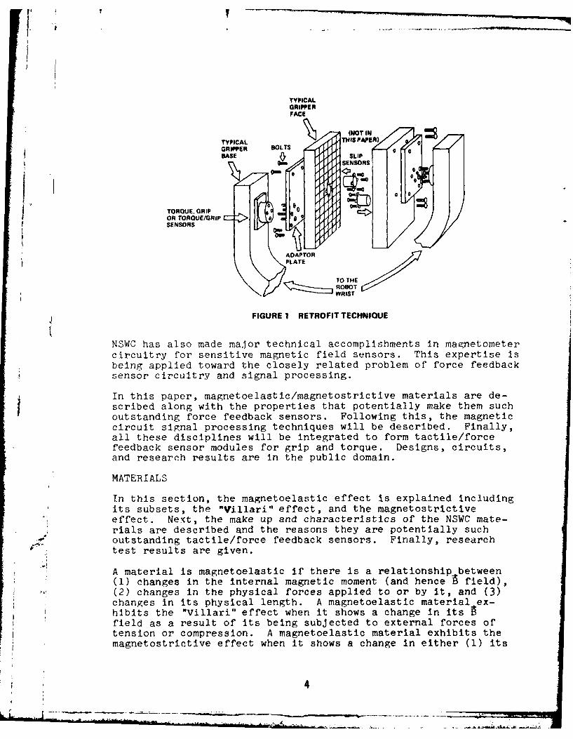
NSWC is developing high performance, simple, rugged, cost effec-tive magnetoelastic/magnetostrictive force feedback sensors formachine tools and robots. (Note figure 1.)

The Navy is facing increasingly severe manpower and skills short-ages. Costs of equipment and complexities of equipment mainte-nance are escalating. To combat this, CAD/CAM, intelligeitautomation, and robotics are depended upon to play a vital role.Tactile/force feedback sensors will be at the center of the Navyeffort.

To optimize its contribution, NSWC is pulling together a range of

disciplines, technical expertise, and experience ranging frommaterials basic research, to signal processing techniques, tomodular robotic sensor designs.

The heart of this coordinated effort is the materials basic re-search. Since the 1960's, NSWC has been performing basic researchin rare earth materials. In recent months, breakthroughs havebeen achieved which permit these materials to be used to push thestate of the art for a range of practical, high performance,tactile/force feedback sensor applications.

3

L i7

TYPICALGRIPPERFACE

(NOT INGRIPPER B3OLTS 00BASE SLIPNm mSENSORS

"o 0

TORQUE, GRIP 0 fie d eOR TORGUE/GRIP o

SENSORS

ADAPTORPLATE

TO THE~zz-zz:JROBOT

WRIST

FIGURE I RETROFIT TECHNIQUE

NSWC has also made malor technical accomplishments In magnetometercircuitry for sensitive magnetic field sensors. This expertise Isbeing applied toward the closely related problem of force feedbacksensor circuitry and signal processing.

4 In this paper, magnetoelastic/magnetostrictive materials are de-scribed along with the properties that potentially make them suchoutstanding force feedback sensors. Following this, the magneticcircuit signal processing techniques will be described. Finally,all these disciplines will be integrated to form tactile/forcefeedback sensor modules for grip and torque. Designs, circuits,and research results are in the public domain.

MATERIALS

In this section, the magnetoelastic effect is explained includingits subsets, the "Villari" effect, and the magnetostrictiveeffect. Next, the make up and characteristics of the NSWC mate-rials are described and the reasons they are potentially suchoutstanding tactile/force feedback sensors. Finally, researchtest results are given.

A material is magnetoelastic if there is a relationship between(1) changes in the internal magnetic moment (and hence A field),(2) changes in the physical forces applied to or by it, and (3)changes in its physical length. A magnetoelastic material ex-hibits the "Villari" effect when it shows a change in itsfield as a result of its being subjected to external forces oftension or compression. A magnetoelastic material exhibits themagnetostrictive effect when it shows a change in either (1) its

~4

physical length due to changes which have been induced in itsjnternal A field, or (2) the inverse-changes in its internalB field which have been induced by changes in its physicallength.

In this paper we are basically concerned with two families ofmagnetoelastic materials; amorphous ribbons - Fe7 0Co1 oB 2 0 (withsmall amounts of silicon and cobalt) and Tb. 2 7Dy, 7 3Fe 2 rods.Both materials exhibit "Villari" and magnetostrictive effects.*The amorphous ribbons are superior in "Villari" effect sensingapplications due to stretching forces and the Tb. 2 7Dy. 7 3Fe 2 rodsare superior in magnetostriction (but they can also performexcellent "Villari" effect sensing in response to compressiveforces).

This materials development was begun when NSWC scientists reasonedthat while rare earth materials possess extraordinary magneticproperties at below room temperatures, it might be possible todevelop alloys and amorphous solutions combining the rare earthswith the more classical ferrous materials to provide practicalnew materials with extraordinary performance properties. Thesematerials can be used at normal room temperature and above. Afternearly 20 years of research into this matter, the materials arenow reaching the point where they are ready for industrialapplications.

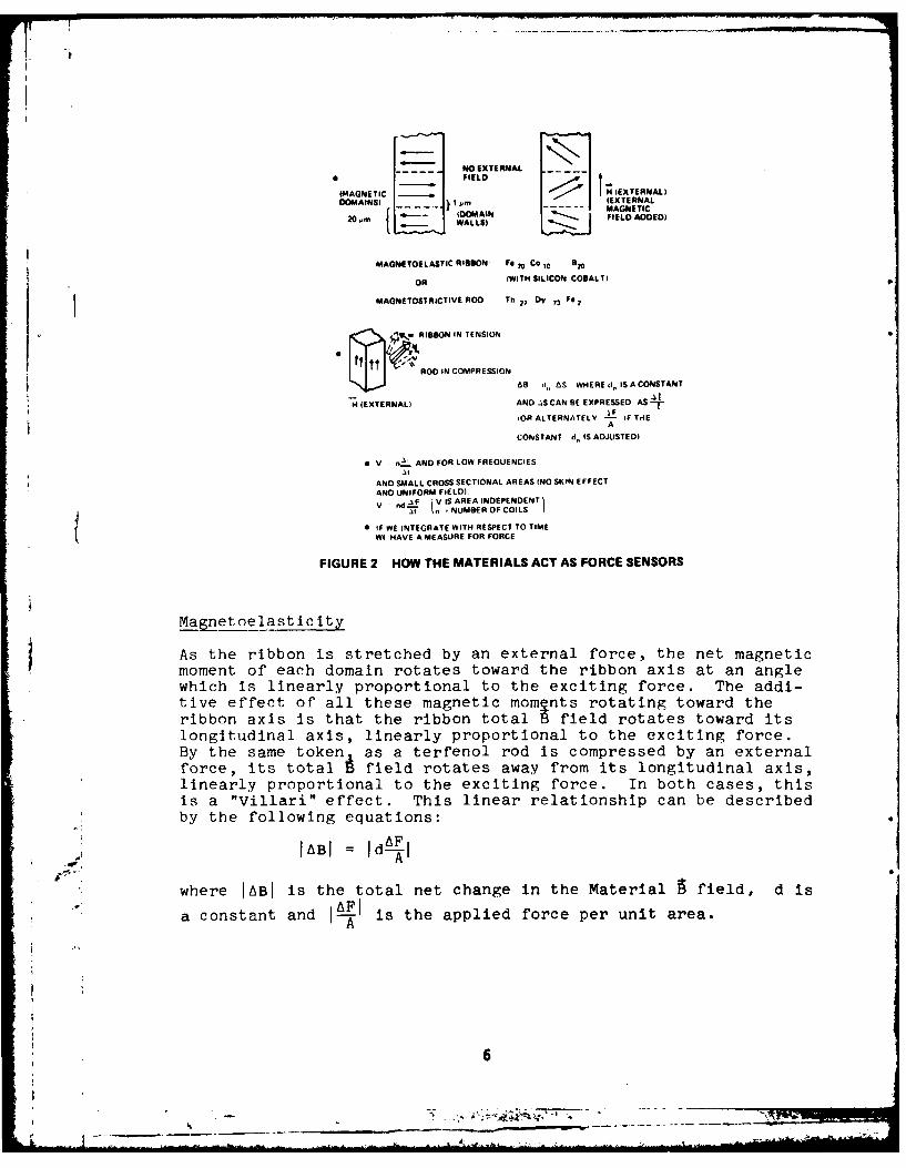
Let us now discuss how these materials act as tactile/force feed-back sensors. As shown in figure 2, the materials are firsttreated so that each internal magnetic domain lines up with itsnet magnetic moment perpendicular to the long axis of the material.At the same time, the net magnetic moment of each domain is pointedin a direction opposite to that of its neighbor's. This leaves thematerial with a total net magnetic moment of zero; thus reducingspurious effects and increasing material sensitivity. If themagnet elastic material is now biased by an external magneticfield H (either by permanent magnetic material or current) themagnetic moments rotate toward the direation of the field. Formaximum linear dynamic range, the bias H field is set such thatthe direction of the net magnetic moment of each magnetic domainis at approximately 450 to the axis of the material.

•Magnetoelastic materials research has been in process at NSWCsince the 1960's. The material "terfenol" (Tb. 2 7Dy. 7 3Fe 2 ) wasdiscovered by Dr. A. E. Clark at NSWC. Dr. H. Savage and staffhave pursued the work in perfecting the material (along withseveral applications patents). Research in another material(amorphous ribbons) was begun at NSWC by Dr. M.Mitchell and hassince been continued by Dr. Kabacoff and staff.

5

II

* FIELD-- 11111]-tHIEEXTENALLMAGNETIC E EXTERNAL)

(OMAINSI - (EXTERNALAMAGNETIC

(DOMAIN FIELD ADDED)20 m WALLS)

MAGNETOELASTIC RIBBON Fe 70 CO to B70

OR (WITH SILICON. COBALT)

MAGNETOSTRICTIVE ROD Th 27 DY 73 F0 2

-IT,- RIBBON IN TENSION

RO IN COMPRESSION

AS 1, , AS WHERE dn ISACONSTANT

H (EXTERNAL) AND .SCAN BE EXPRESSED AS--iOR ALTERNATELY ;IF THE

A

CONSTANT d, IS ADJUSTED)

0 V n"L AND FOR LOW FREGUENCIES

AND SMALL CROSS SECTIONAL AREAS (NO SKIN EFFECTAND UNIFORM FIELD).V - nd AF V IS AREA INDEPENDENT

.7 I. - NUMBER OF COILS I

* IF WE INTEGRATE WITH RESPECT TO TIMEWI HAVE A MEASURE FOR FORCE

FIGURE 2 HOW THE MATERIALS ACT AS FORCE SENSORS

Manetoelastic ity

As the ribbon is stretched by an external force, the net magneticmoment of each domain rotates toward the ribbon axis at an anglewhich is linearly proportional to the exciting force. The addi-tive effect of all these magnetic moments rotating toward theribbon axis is that the ribbon total field rotates toward itslongitudinal axis, linearly proportional to the exciting force.By the same token as a terfenol rod is compressed by an externalforce, its total A field rotates away from its longitudinal axis,linearly proportional to the exciting force. In both cases, thisis a "Villari" effect. This linear relationship can be describedby the following equations:

IABI = AdF1A

#" i~iwhere IABI Is the total net change in the Material 9 field, d is

, a constant and is the applied force per unit area.

6

-. ----. -

AF, YAl

* where y is the Young's Modulus of the material in psi and 1is the material change in length per unit length.

-kI = djAHf where (AHI is an externally applied magnetic field.

(One should recall that = A i where is the material- permeability (u OP.

Referring to figure 2, if we wrap either an amorphous ribbon or a* terfenol rod with coils of insulated wire and send current through

* the wire, a A field will be superimposed on the A field already inthe material. This will cause the amorphous ribbon and terfenol

*rods to expand or contract depending on the product of the cur-rent and the number of coils. This magnetostrictive property ismost pronounced for terfenol rods (see figure 3).

A

CLOSED PATH OF

S• INTEGRATION

4 -4

FIELDSCANCEL IN THESE REGIONS

FIELDS REINFORCE IN THIS REGION

NOT TO SCALE

FIGURE 3 H&B FIELDS IN THE MAGNETOSTRICTIVEROD

Again, we can use the j_ dlP/Af relationship. But AA Pwhere ~vi use - 4 x 10'(8) since u terfenol - 8.'"

The question then becomes how large can we make AD? Let us illus-trate by picking a few numbers. Using a current of 1 amp, a rodlength of 2 inches (5.08 cm), .25 in. diameter (.635 cm) and with2000 turns of wire around it, we will get:

• dl- I 2000 (1)

(where length is in meters). And referring back to figure 3, thissimplifies to A B (.0508)- 2000 (I amp)

Thus = .126 webers/m2

IBi = djAP/Aj; d = .25 x 10-7 webers/newton for terfenol and

1 lb = 4.44 newtons.

So = 35.9 lbs or 159 newton,

Again back to our equation

AAI = dI-L whei d - 8.6 X 102 webers/m 2

o~r

AB = 8.6 x 102/ 2-in

But AB .126 webers/m2

Thus Z = 2.93 x 10 -4 in (7f44 x 10- ' cm)

Magnetostriction

Of course one can see that increasing the product of the currentand windings increases bot: the force and the magnetostrictivetravel. (Magnetostrictior of .001 in. per inch is easilyachievable for terfenol.)

Force Sensing

There are essentially tw/ methods for force sensing using magneto-elastic materials, one I technique which measures the total forceacting on the sensor an( one which measures the rate of change ofthe force acting on the ensor.

*Values and equations rom Dr. Howard Savage's notes 4/13/81.

8

7 7,

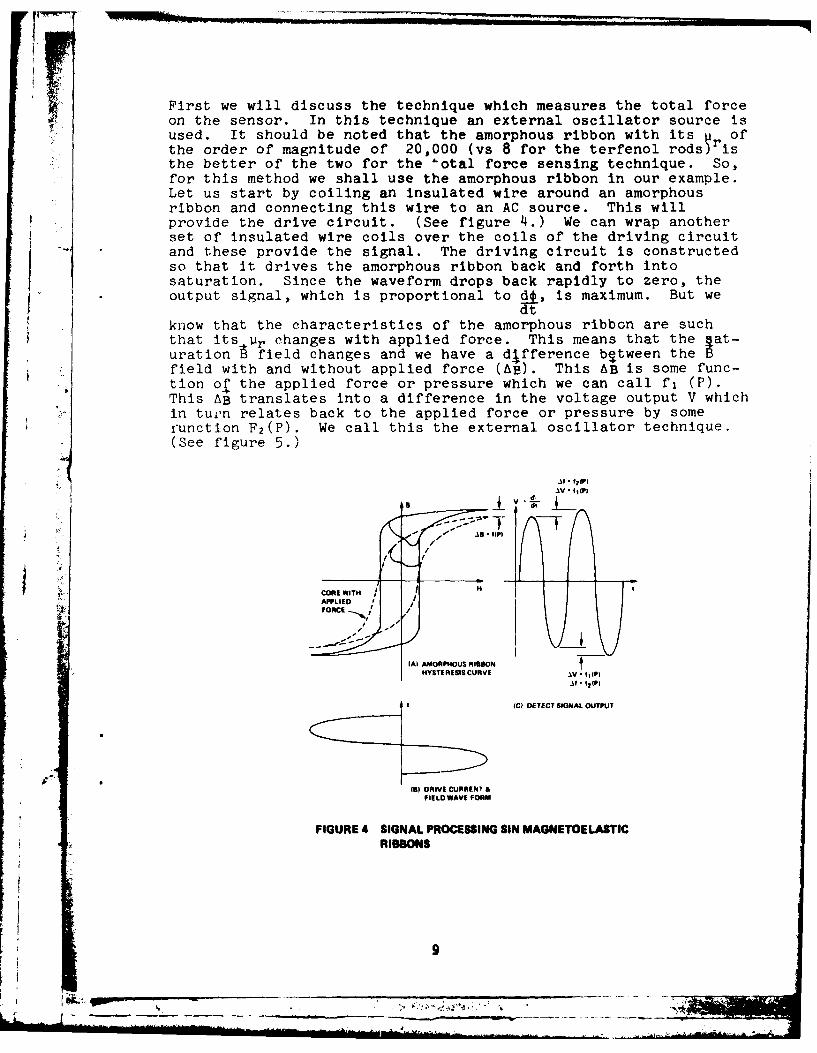
First we will discuss the technique which measures the total forceon the sensor. In this technique an external oscillator source is

used. It should be noted that the amorphous ribbon with its r ofthe order of magnitude of 20,000 (vs 8 for the terfenol rods) isthe better of the two for the 'otal force sensing technique. So,for this method we shall use the amorphous ribbon in our example.Let us start by coiling an insulated wire around an amorphous

ribbon and connecting this wire to an AC source. This willprovide the drive circuit. (See figure 4.) We can wrap anotherset of insulated wire coils over the coils of the driving circuitand these provide the signal. The driving circuit is constructedso that it drives the amorphous ribbon back and forth intosaturation. Since the waveform drops back rapidly to zero, theoutput signal, which is proportional to de, is maximum. But we

dt

know that the characteristics of the amorphous ribbon are suchthat its Pr changes with applied force. This means that the §at-uration A field changes and we have a dIfference between the Bfield with and without applied force (AB). This AB is some func-tion of the applied force or pressure which we can call f, (P).This AB translates into a difference in the voltage output V whichin tujn relates back to the applied force or pressure by somei'unction F 2 (P). We call this the external oscillator technique.(See figure 5.)

. -flP). /

CORE WITH /APPLIED

FORCE -

IA1 AMORPHOUS RIBBONHYSTERESIS CURVE AV •I

1P)

l,(PI

(C? DETECT SIGNAL OUTPUT

(BI DRIVE CURRENt &FIELD WAVE FORM

FIGURE 4 SIGNAL PROCESSING SIN MAGNETOELASTICRIBBONS

L9-

I

390 A0 10

14O KND^v 10 K

FIGURE S THE SEPARATELY EXCITED OSCILLATOR

Next we will discuss the technique which measures the derivative

of the total force (or pressure) with respect to time (). This

technique depends on the rate of change of flux 0

= f . d (s = area of ribbon or rod cross section). The

governing equation is:

V = n d¢ n = number of coilsdt V = voltage output

Looking at figure 2, we can see that we have essentially a passivesensor with one set of coils (no driving circuit). It will oper-ate at very low frequencies (to DC), those of the robotic tactileforce itself. At these low frequencies, and with the small crosssectional areas of the ribbons and rods (typically .006 in 2 ), thereis virtually no skin effect or magnetic hysteresis and theequation simplifies to:

V = n AB d's (A' d-)dt AFs

So: V = n - d2 -d A (S = A)

"V dFV =nd 2 dt

dF

Thus we can see that the voltage is proportional to the term

(o ) and the integral of 112 V dt yields the total force.(or Idt-)adteitga1

The high efficiency of the rods and ribbons (mechanical work onthe material compared to the change in magnetic field AB) makesthe derivative sensor practical.

10I ________________________________________ ________________________

r Generally the force derivative sensor provides a relatively lowvoltage, high power output. And, comparing figures 2 and 3, one

V; can see that when a terfenol rod is used there is the option of itacting either as a sensor or actuator. On the other hand, theexternal oscillator technique yields higher output voltages andthe sampling time is not critical (since total force is measured).Clearly, the preferable technique depends on the application.

Let us now discuss why these materials are potentially such goodforce feedback and tactile sensors.

Outstanding Sensitivity

Both the ribbons and the terfenol rods have demonstrated outstand-ing sensitivity. A 0.8 ratio for magnetomechanical coupling hasalready been produced at NSWC for both the rods and amorphous rib-bon and the value is expected to climb to 0.9. This 0.8 value isthe ratio of the output voltage to the voltage equivalent of theforce applied to the material. A 40 mV/V ratio was previouslyconsidered excellent.

Outstanding Dynamic Range

A conservative estimate of the ribbon's linear region for dynamicrange is +1,000 psi. It should also be noted that experiments atNSWC (for-underwater pressure sensors) have indicated that it ispossible to resolve .004 psi in a background depth of 266 psi.This means that theoretically we can expect 10 log (266/.004) =48.2 dB volts. 30 dB power or 15 dB volts is normally consideredto be excellent. The terfenol rods have a dynamic range 2 timesthat of the ribbons and are prestressed to 2,000 psi.

No Observable Mechanical Hysteresis

The amorphous ribbons and terfenol rods are, for all intents and

purposes, completely recoverable. This recoverability extends towell beyond 2 or 3 times the +1,000 psi linear dynamic range ofeach.

Outstanding Linearity

Graphs for both experiments conducted by Japanese investigators,K. Mohri and E. Sudoh, showed outstanding linear response and

* • this linearity has been duplicated at NSWC by investigatorJ. F. Scarzello.***

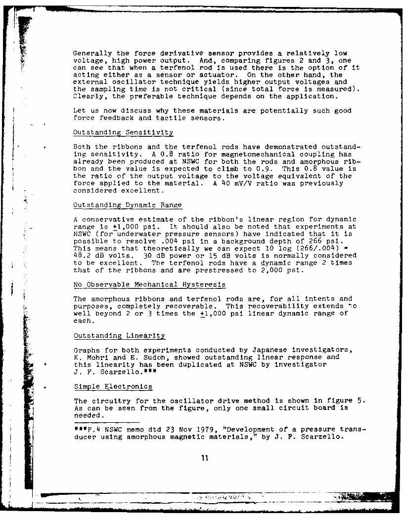
Simple Electronics

The circuitry for the oscillator drive method is shown in figure 5.As can be seen from the figure, only one small circuit board isneeded.

***P.4 NSWC memo dtd 23 Nov 1979, "Development of a pressure trans-

ducer using amorphous magnetic materials," by J. F. Scarzello.

11

.~ * .~A

Tough, Inexpensive, Corrosion Resistant and Radiation HardenedMaterials

The amorphous ribbons are tough and can stand up to 20,000 psi(13,764 newtons/cm 2 ). The rods, when prestressed to 2,000 psi(1,376 newtons/,cm 2 ) in a metal can, are also tough. Both materialscan be mass produced inexpensively. Both are extremely resistantto corrosion and radiation. But there are aspects of the materialwhich require additional investigation and/or are a bit troublesome.

Stray Fields and Voltage Offsets

This is a problem, particularly for the amorphous ribbons becausethey have such a high - (magnetic permeability) and because theyare driven by the "external oscillator" technique. NSWC ispursuing three techniques to deal with this problem: (1) puttingmagnetic shielding material around the ribbons, (2) using 2 setsof symmetrical windings so that the errors are self cancelling,and (3) using filtering and digital signal processing techniques.

Noise in the Ribbon (when operated as part of the external driveoscillator system)

4This noise tends to restrict the available dynamic range of thesystem. As a result, the materials experts at NSWC are continuingto work on improving the material and considerable progress hasbeen made. It has also been noted that the ribbons tend toresonate magnetostrictively, so selecting the proper drivefrequency can lower noise considerably. 15 KHz has yielded goodresults.

Brittlenpss in the Terfenol Rods

Very recent experiments at NSWC have resulted in terfenol rodswhich can stand 2,000 psi (1,376 newtons/cm 2 ) in tension (inaddition to high compressive capabilities). This representsstill another improvement in the breed.

Low Ur In the Terfenol Rods

Low ur and high magnetostrictive capabilities go hand in hand soonly limited progress can be made in this area. This means thatthe terfenol rods must act as derivative sensors and cannot bedriven by the separately excited oscillator technique.Temperature Stability

This has not been fully tested though stability to 100 0 C isanticipated.

12

__ _ _ _ _ _ _ _ _ _ _ _ _ _ _ _ _ _ _

SIGNAL PROCESSING

In this section, signal processing techniques will be outlinedincluding both the oscillator drive technique and the derivativemethod. Some of the expected signal processing problems andtheir usual methods of solution are addressed.

The oscillator drive method is the main signal processing tech-nique to be used in the grip, torque, and grip/torque modules.

As mentioned above, this method measures the total force or torqueas the case may be and it is simple, sensitive, and accurate. Inaddition, this technique is well understood at NSWC since it wasdeveloped for magnetometers in underwater mine and space applica-tions, and it has resulted in many major publications and patentsdating back to 1970. (For example, a magnetometer designed jointlyby NSWC and NASA Ames Research Center was a part of the equipmentdeployed on the lunar surface in the Apollo 16 Mission.)

The Relationship of Magnetometers to Robotic Force Feedback Sensors

In a magnetometer, the magnetically active element (in our case anamorphous rib on) has its A field changed by an intruding magneticfield. This X in turn changes the magnetic reluctance of theamorphous material. If the material is being excited by an oscil-lator drive, as an intruding magnetic field adds to or subtractsfrom the magnetic field in the magnetometer core, output voltagewill be affected. But as we noticed earlier, the same effect willoccur if the ribbon is physically stressed. Thus the oscillatordrive signal processing technique is equally applicable to forcefeedback sensors and magnetometers.

A Brief Description of how the Oscillator Drive ProcessingTechnique Works

A key factor is the current/field wave shape in the driving cir-cuit coils. This wave shape is such that the current/field buildsto a peak and then rapidly drops to zero. The resulting largedcan be used to provide a voltage output which is a function of

adtthe force on the ribbon (see figures 4 and 5).

* As the sensor ribbon is stretched by a robotic force or torque,* the slope of the -l curve becomes steeper and the output voltage

greater. Also, inductance is proportional to the slope of thiscurve, so a circuit which will produce a signal proportional toinductance will produce a measurable signal.

The central component of the circuit is an operational amplifier(op-amp). As a result of high amplifier gain, A, and high inputimpedance, it can be shown that the output voltage is related tothe input voltage by the ratio of feedback and input impedance.

13

= (Zb)

b a va

Suppose the input voltage is sinusoidally varying:

Va = V sin(wt)

Its magnitude is given by

IV a I V

If the input component is a resistor, and the feedback componentan inductor: then

Za = R Zb = JwL

and

IVb (wV) LI~ ~~ ~b Rhsi hc st nutne

Thus a signal is produced which is proportional to inductance.

If both ribbons are pre-tensioned, an additional force willincrease inductance in one coil, and decrease inductance in theother, both by L (figure 5).

The voltage magnitudes at points V 1 and V2 are given by

V Vw (L -AL) Vw (L +AL)

The orientation of the diodes cause the dc levels

V = Ivil V 4 = -IV21

The final op-amp adds V3 and V4 . 3IV0 = -(b) (V3 + V4 )

,* Combining the above

Vo (2Vw Rb)ALR Ra

14

___

This is a signal proportional to the difference in inductancecaused by an imbalance in ribbon tension (sensor ribbon comparedto a ref. ribbon). This simplified circuit is expanded to includea zero adjustment and ideal diodes.t Specific component valuesare shown in figure 5.

The Vo from the circuit shown in figure 5 can now be furtherprocessed. We can pick up the RMS voltage output (using perhapsa simple square law detector). In this process, the equationV° '.44 N2 f BA x 10

-8 volts

N = number of windingsf = frequencyA = area

is a good estimate of the RMS value we would expect. Since aforce on a robotic sensor int rduces a change in B using, once

again, the equation [A J = dI.jI, we will get a change in the

total voltage output of approximately:

Vrms = 4.44 N2f B A x l - volts

sinceIABI = l

dIA-I

AV x10-8

IAI =4.44 N 2 fd

Thus simply measuring the RMS voltage output will pr-' de u ththe information we reed to solve the force, or toTi'., direcciY.

The derivative technique can also be used for signal processing inany of the magnetoelastic/magnetostrictive robotic force feedbacksensors. A2 mentioned above, in the derivative technique the

equation V = n ! applies or V = n !L dAFdF dt dt

V = n dI-1. So, again, we are dealing with the rate of force

application.

tFrom "Progress Report Magnetoelastic Sensor Development," 6/15/81thru 8/15/81 Prof. R. DeMoyer and Prof. E. Mitchell, U.S. NavalAcademy, 9/15/81, pp. 11-13

-15

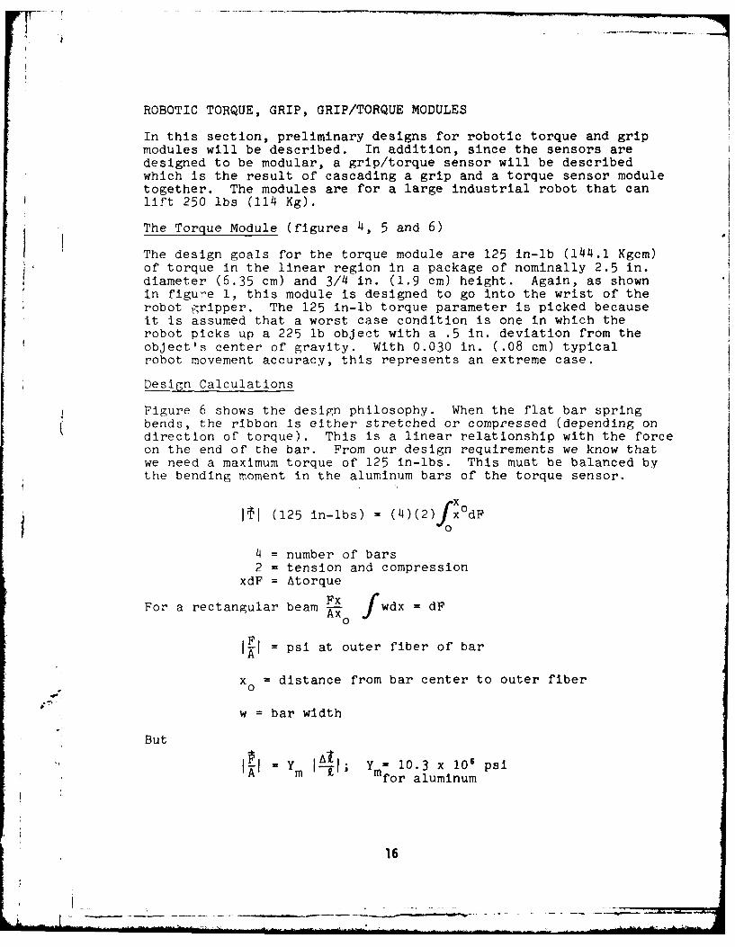
ROBOTIC TORQUE, GRIP, GRIP/TORQUE MODULES

In this section, preliminary designs for robotic torque and gripmodules will be described. In addition, since the sensors aredesigned to be modular, a grip/torque sensor will be describedwhich is the result of cascading a grip and a torque sensor moduletogether. The modules are for a large industrial robot that canlift 250 lbs (114 Kg).

The Torque Module (figures 4, 5 and 6)

The design goals for the torque module are 125 in-lb (144.1 Kgcm)of torque in the linear region in a package of nominally 2.5 in.diameter (6.35 cm) and 3/4 in. (1.9 cm) height. Again, as shownin figure 1, this module is designed to go into the wrist of therobot gripper. The 125 in-lb torque parameter is picked becauseit is assumed that a worst case condition is one in which therobot picks up a 225 lb object with a .5 in. deviation from theobject's center of gravity. With 0.030 in. (.08 cm) typicalrobot movement accuracy, this represents an extreme case.

Design Calculations

Figure 6 shows the design philosophy. When the flat bar spring

bends, the ribbon is either stretched or compressed (depending ondirection of torque). This is a linear relationship with the forceon the end of the bar. From our design requirements we know thatwe need a maximum torque of 125 in-lbs. This must be balanced bythe bending moment in the aluminum bars of the torque sensor.x

I I (125 in-lbs) = (4)(2)f xodF

4 = number of bars2 = tension and compression

xdF = Atorque

For a rectangular beam Ax fwdx = dF

JEJ= psi at outer fiber of bar

x= distance from bar center to outer fiber

w = bar width

But

=~ =m 10.3 x 106 psifor aluminum

16

HO SIn OSN

aFLAT o num /AV IT

=T.. PRO CMeE O

;MMOUSI DREAVESURFAE I OCL

FIGURE 6 ORU SENSOR

and~~~~ ~MPOV foMIopouSibosIO5N O~ni

MISO ESOLets dd o 25 x106i/in fr adEsivoshar

125 ~ ~ ~ ~ IIN 8 xOd =8l03(5)MSd

2LA WRN 125010" AV ISACWX 0 ME A43.20OIC~a wemkMtAi n idi utb 1 N hc. Ti en

thatif ur eectonic ha 30 B dnami rage, e cn pikAu

125s in-l o 25 i-lb /in the linsea to25h i-besigthrnn

1 - - -- x- (03)5)

f Ax If-

We know Vrms - 4.44 N2f BA x 10- 8 volts (CGS units)

B - d F/A

for Mks units use

F lb ttd = 11.1 Fi 1

with f = 15 KHz; Vrms required - .lmV

we get the design relationship

.0135 = F lb N2 or .00614 = FkgN 2

We will use a ribbon .2 in. wide by .002 in. thick with 0 to+1,000 psi linear dynamic range. So, at its maximum stress, itwill experience (1,000) .002(.2) = .4 lb tension or compression.This corresponds to .125 in-lbs torque on the beams. To get downto .025 in-lbs (28.9 gmcm or 37 dBV dynamic range), we need.00008 lb sensitivity in the ribbon:

.00008 N 2 = .0135

N2 = 168; use N2 = 170 turns

It will be a challenge to get the electronics to handle suchsensitivity.

At this point we will examine the results from a test prototypetorque sensor. This prototype was built oversize so as to facili-tate testing and modification. It is essentially patterned on theconcept shown in figure 6.

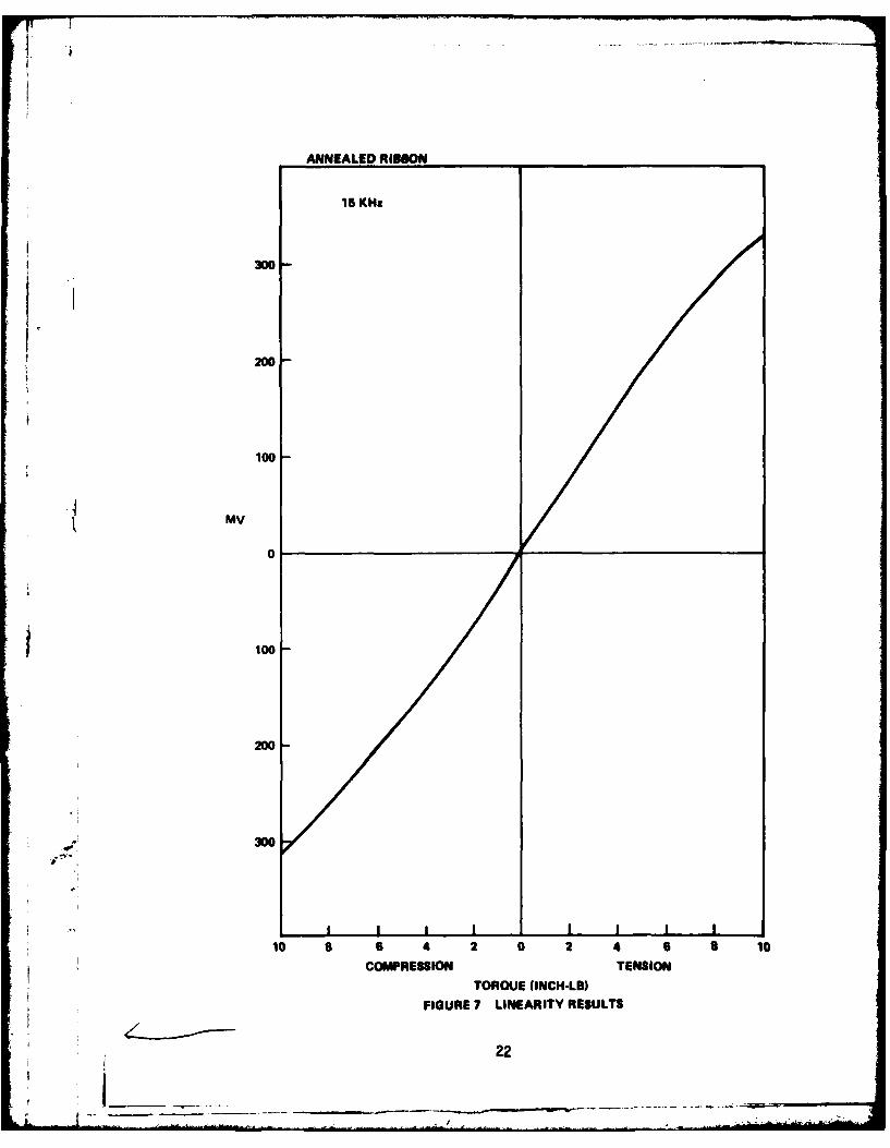
Results (see figure 7)

At 10 KHz, inductance increases with tension up to a point afterwhich it remains constant. This is true for both annealed andunannealed ribbon.

Slight deviations from linearity at the curve extremes areprobably due to the adhesive yield in shear.

Using annealed ribbon, the change in inductance effect with tensionis reversed from the unannealed version.

ttMeeting 3/23/80, Dr. Howard Savage, J. M. Vranish.

18

.J.....

The annealed ribbon can take high signal levels without saturation,and the output is a reasonably linear function of applied load inboth tension and compression.

Conclusions

The annealed ribbon excited at a frequency near its resonanceexhibits desirable properties: near linearity, large dynamic range,and high level output. The phase shift between the annealed andunannealed is due to the fact that annealed and unannealed ribbonsresonate magnetostrictively at different frequencies.

Future Work

A magnetic return path should be installed to determine if theeffects of external iron proximity can be totally eliminated.

Many trade-offs include:

Signal levelsFrequencyNumber of turns on coils

All components must be miniaturized in order to construct apractical torque/force sensor.tit

We can now show the design approach that will be taken on the gripsensor. This is the same as the torque sensor except the forcecomes straight down and the ribbons are on the top and bottom ofthe bars rather than the sides as in the torque sensor.

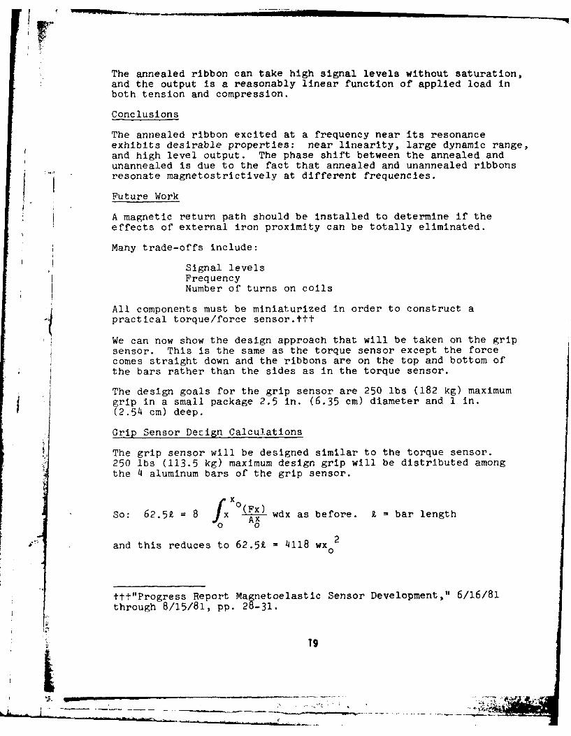
The design goals for the grip sensor are 250 lbs (182 kg) maximumgrip in a small package 2.5 in. (6.35 cm) diameter and 1 in.(2.54 cm) deep.

Grip Sensor Decign Calculations

The grip sensor will be designed similar to the torque sensor.250 lbs (113.5 kg) maximum design grip will be distributed amongthe 4 aluminum bars of the grip sensor.

So: 62.5k = 8 (Fx) wdx as before. i = bar length0f 2

and this reduces to 62.5k = 4118 wx 2

ttt"Progress Report Ma netoelastic Sensor Development," 6/16/81through 8/15/81, pp. 29-31.

1I9.,-. J

usingZ = 1 in. and picking w - 3/8 in., we get a bar thicknessof .4 in. (1.02 cm). Our electronics relationships remain thesame as for the torque sensor.

.0135 = Flb N2

If we use .008 lb in our ribbon as the minimum force to pick upat .lmV rms signal output voltage,we will need 170 coils asbefore.

Future Directions

During the first year, NSWC will continue to develop and refinethe sensor modules. This will include optimizing the amorphoussensor material for robotic applications.

In the second year, the sensor modules will be interfaced with theNSWC robot to iron out the control theory and vision coordinationquestions. Also during this year, a gripper will be designed forthe removal of high tension fasteners from Navy missiles.

In the third year, a gripper will be built and the sensor modulesinterfaced.

In the fourth year, the gripper will be interfaced to a heavy dutyindustrial robot and the combined system tested in a Naval WeaponsStation.

SUMMARY AND CONCLUSIONS

In summary, we have described the NSWC Program for developing highperformance, simple, rugged, cost effective magnetoelastic/magnetostrictive force feedback sensors for machine tools androbots in CAD/CAM operations. We have shown that the NSWC Programis a comprehensive program including basic materials research,signal processing, and robot sensor modules. We have outlined thematerials characteristics, the signal processing techniques, andthe robotic sensor designs. The basic research has been success-fully completed, and practical force feedback sensors for robotsare being constructed and debugged. The NSWC Program will signifi-cantly advance the state of the art in force feedback sensors.

BIBLIOGRAPHY

1. For materials Introduction, U.S. Navy Journal of UnderwaterAcoustics, Vol. 27, No. 1, Jan. 1977 "Introduction to HighlyMagnetostrictive Rare-Earth Materials," by Dr. A. E. Clark.

2. For Terfenol Rod Application read "The Robotic Sensor/Gripper,"J. Vranish, NSWC, Feb. 1981.

20

L L

3. For Brown Oscillator Circuits - See U. S. Patent 3,649,908,March 1982, and the publication entitled "A Miniature FluxgateMagnetometer with Subgamma Noise," presented at IEEE IntermagConference, Kyoto, Japan, April 1972.

4. Handbook of Physics, 1957, McGraw Hill.

I.

21

Z!

ANNEALED RIBBON _____________

15 K~a

200

100

MV

0

100

200

10 a 6 4 2 0 2 4 6 S 10

COMPRESSION TENSIONTOROUE (INCH-LB)

FIGURE 7 LINEARITY RESULTS

22

IMODERN CONTROL TECHNIQUES APPLICABLE TOTHE SPACE SHUTTLE MAIN ENGINE

T. C. EvattRockwell International Corporation

Rocketdyne Division

r

Next page Intentionally left blank.

23

. . .* .

AD P 0026MODERN CONTROL TECHNIQUES APPLICABLE TO

THE SPACE SHUTTLE MAIN ENGINE

T. C. EVATT

ROCKWELL INTERNATIONAL CORPORATIONROCKETDYNE DIVISIONSYSTEMS ANALYSIS

CANOGA PARK, CALIFORNIA 91304

INTRODUCTION

Historically, development of liquid propulsion rocket controlsystems has utilized classical control techniques to regulatethrust and mixture ratio. The approach taken here is to modelthe Space Shuttle Main Engine as a linear-multivariable systemwhose parameters vary with engine operating environment. Onlyinputs and noise corrupted outputs realizable at an actualengine are considered. The engine control objective centeredon controlling preburner temperature, mixture ratio and thrust(combustion pressure). An eighth order linear model with twoI actuators (valves) and their associated dynamics is derived toapply optimal linear. quadratic design methodologies to controlfuel turbine inlet temperature gradients. The design metho-dology selected to investigate and develop a feedback con-troller for these temperature grad ients is the Linear QuadraticGaussian (LQG) design philosophy.' This method is a syste-matic method of regulator control using a Kalman-Bucy filter(state estimator) to determine plant states from measured para-meters. A subset of the LQG design methodology, the LinearQuadratic Regulator (LQR) will be derived for an SSME deter-ministic model at one design point and graphical resultspresented.

The use of this modern control methodology represents anadvance in the design philosophies used in rocket engine con-trol systems. At the time of the SSME control system design inthe early 1970's, attention was given to both classical andmodern control system design methodologies. The state of theart, however, was not mature enough to use the modern controlsystems design approach for the SSME. As a result, an advancedapplication of the classical methodology was selected for thecontrol system design.

With the foreseeable increasing performance demands on theSSME, LQG control methodology that relies on linear quadraticsynthesis of regulators at different operating points is beingapplied to design an improved control system. Many papers havebeen written on engine control using Linear Quadratic Design

25

techniques. Hoff and Hall2 ,3 have discussed a control designmethodology for turbine engine control synthesis using regu-lators at a number of power levels at sea level, static condi-tions. Taiwo discussed a method of turbine controllerdesign using Zakain's method of inequalities. Merrill hasused sampled data regulators to design multivagiable controllaws for jet propulsion. Michael and Farrar0 discussed apractical and systematic linear quadratic synthesis procedure.The regulator design techniques, however, rely on full-state

availability. -.

This paper is divided into four sections. The first sectionintroduces the SSMEA'rocket engine and the techniques used tosimulate the dynamics of the SSME including linear model deri-vation. A discussion of actuator dynamics and their effect oncl. loop response is also presented. In the next section,the LQG, technique is briefly discussed with a more detaileddescription of the Linear Quadratic Regulator. A procedure isdiscussed for choosing the LQR weighting matrices. Conclusionsand recommendations follow.

SSME TURBOPUMP ROCKET ENGINE

INTRODUCTION

With the advent of the space shuttle concept in the late 60's,it became apparent that a reusable and reliable engine designwas needed. The high performance requirements of the SpaceShuttle Orbiter demanded a new state of the art in liquid pro-pellant rocket engine design. The Space Shuttle Main Engine(SSME) design uses a staged combustion power cycle (Figure 1)coupled with high combustion chamber pressures. In the SSMEstaged combustion power cycle, the propellants are partiallyburned at low mixture ratio, very high pressure, and relativelylow temperatures in the preburners to produce hydrogen-rich gasto power the turbopumps. The hydrogen-rich gas steam is thenrouted to the main injector where it is injected, along withadditional oxidizer and fuel, into the main combustion chamberat a higher mixture ratio and pressure. Liquid hydrogen isused to cool all combustion devices directly exposed to contactwith high-temperature combustion products. An electronicengine controller automatically performs checkout, start, main-stage and engine shutdown functions.

The SSME was developed especially for the Space Shuttle OrbiterVehicle, which uses three engines for launch. The SSME is areusable, high performance, liquid propellant rocket enginewith variable thrust. The engine is ignited on the ground atlaunch and operated in parallel with the solid rocket boostersduring the initial ascent phase and continues to operate forapproximately 520 seconds total firing duration. The require-ment for 55 missions totaling 7.5 hours of cumulative operating

26

J.

Mi 0 zL

U.)

mLL LA0

N LoA

0-1-

00

000uij 2!:

z L ii

tr

-JAd

ii.

IL 0- LL.

27

Ful L filbief

DUCT LEGEND Ou:?FLUID FLOW PAY"

-- Ow- mECI4AICAL LINK

.... 0 CONTROL I.O-Ct

L11--0-00- PEAT TRANSFERt LOW

PRESSURE AROS INDICATE DIRECTION PRESSUREFUEL PUftP OF PROCESS FLOW OXIDIZER

LOW LOW-PRESUR AC SURECTUR111,19TURSINE

I apui* XIDIZEROXIDIZER-aPU

VALVEVA4.vE

FUEL OXIDIZER

INJECTORII CTOPRCOMBUSTOA C SO

FIGURER 2 - NAO MDE FO DAGA28L X , *

ZER.

-UIN -.------- R - U---"E

time with varying thrust levels represented the first signi-ficant requirement for a reusable liquid rocket engine. TheSSME is a very efficient engine with a specific impulse ofapproximately 455 seconds at rated power level (RPL) (470,O00pounds of thrust altitude). The two stage combustion isapproximately 99.96% efficient. The main chamber combustir.pressure is approximately 3000 psia at rated power level. theturbopumps are direct drive, i.e., they have no gear tains.Another interesting feature of the SSME is that it ;.As'.s headpressure to supply the energy to start the engine. T'-ere areno start tanks, turbine spinners, or pyrotechnics ir.,olved Inengine start. Electrical igniters are supplied in t!.j fuel andoxidizer preburner and the main combustion chamber to initiatecombustion.

Each of the rocket engines operates at a pt.Ature ratio of 6:1,and over a throttling range of 109%-651'RPL. This provides ahigher thrust level during lift off" and the initial ascentphase, and allows orbiter acceleration to be limited to 3gduring the final ascent phase. The engines are gimballed toprovide pitch, yaw, and roll control during orbiter boost phase.

SSME HYBRID SIMULATION MODEL

The first stage in designing a feedback control law is toderive a set of differential equations that describe the systemresponse as accurately as possible. The SSME hybrid modeldeveloped by Rocketdyne on the AD-10/PDP-11 computer is thesimulation model used in this study. The engine system analogsimulation model is constructed on a component basis. Indivi-dual turbines, pumps, heat exchangers, and fluid flow passagesare characterized by equations defining component variations,dynamic relationships, and interface requirements. The systemsimulation includes all static and dynamic formulations thatare considered of importance in accurately representing overallstart, mainstage control, and cutoff behavior of the engine.

The hybr-;d model contains three subsections that are used todevelop the basic building blocks to represent all phenomena ofsignificance. The engine fuel flow system involves all physi-cal processes where hydrogen in a gas, liquid, two-phase, orsuper-critical state is handled. The oxidizer flow portion ofthe engine system involves the physical processes where oxygenis handled by the engine system prior to being involved- in anycombustion process. The hot-gas portion of the engine systemsimulation includes all component processes that involve hand-ling oxygen/hydrogen combustion products. This model containssimplifications which include perfect gas law assumptionsinstead of National Bureau of Standards Property Tables, curvefitting of some functions, and linearization of second-ordernonlinear effects. A schematic of the simulation program isshown in Figure 2.

29

---__ _ _

The analog model description represents SSME dynamics and isapplicable for simulating engine start, throttling, and cutoffdynamics at nominal conditions. The analog model differentialequations are used to develop the control linear model used insubsequent sections of the paper.

CONTROLLER REQUIREMENTS

The SSME control system is designed to meet or exceed all per-formance control requirements set by the Contract End Item(CEI) specification. Typical CEI requirements encompass theperformance criteria for startup, mainstage, and shutdown(Table 1). As can be observed in Table 1, all CEI controlrequirements are met or exceeded by the present controller.

For this study, CEI design requirements will be the ultimategoal with the added goal of minimization of temperature gradi-ents (F/s) in the preburners. Excessive temperature gradients(spikes) during engine start/cutoff can cause localized crack-ing of turbine blades (e.g., shortening of turbine blade life).

In summary, the SSME controller requirements for this study are:

1. Design a multivariable control loop which willbe capable of performing control functions on asimulated (hybrid) SSME and demonstrating super-ior performance against existing SSME controls.

2. Develop the above multivariable control loopwith the added design goal of minimizing turbineblade metal thermal gradients (thermal shock;F/s) on the SSME.

MODELING TECHNIQUES

Introduction

The solution for a nonlinear set of differential equations isdifficult or impossible to solve analytically. An approachthat will allow an approximate solution to the process equa-tions taken from the SSME hybrid model is called small distur-bance thlory, small perturbation theory, or lineari-zation.8,1 Initially, a set of steady state operating con-ditions is found from an engine balance. These determine thevalues of the state and control variables needed to maintainthe engine at the steady state operating conditions. The pro-cess equations are then linearized about the engine design

* " point. The following sections describe the linearization pro-cedure for a general set of nonlinear equations and then applythe result to the SSME analog equations discussed previously.

30

no

C, 0 CL - L N -C I-w0~~ ~ ~ 10Ni W r

4n I. In (A tA

ki -j 40 01 0 -

ILi ot-. bet o -" 0KI.- 00000 III -~ 0 4 . YW 4 -j

01 CID w- 0. Un LI 00, C C, ;no 0. Lo CA &n 0#A Wo Won .0o

COY- t"0 -Z +n 0. oni C4 L

0-0

L& taC.j 0

0~ -C i e 0 09X x 0 &A Z 00Ln 4 C In+1~.

In (,o) L.. r. K n C- CI4

In 0 0 U -Io~~~L a4 -a ON* ..0

I- $A .- in u. n- O.

Li I- n - t-In L1IA ccnI =W L* =a M K j U 6Li

In I. I n # i4 ==O M o = IIn14A .- c 1 .- - kI n I Z . m .-. I .

C 0. .1 w so CD _j C0 m .0-j'~.0 CJ ca a0.J- I .0 11 l K

a 000 0u 00oW In In *0n LA LI; Vi C;~ O n -C~ 00'

*jW -+I,,. .N*. O .0 CY T.I Pn

-C 2. P - .J +. - C.Iw,~ N -nn-

16 a a Or CwCLL) -I j L

C, ~ - " 2.69al 8. In W InX

La Ca fi A. C Lu i mw' a I to- 0. 3. Gn . 0.

#M -n . "41 o 0 CD I- w ~ w. oc K1 o

n - '# w0 m In0. W-A : m I - 0 3

= -0 . aI 00 a i = " W 00W3=Sa 1W ch L W"

.. L.8 " I - W -WOaWp- W W 0a -An 4.1W i "0 3 4A -1 0m Cal uaawa us (oa. M "a. #A. mA jb- LIJ _a ~ O.IJ. S MI

a-c.I-- x.a ~ .. . "ACO- o 0 Ws~. IL .. IL

IIC mm ,-- X. 4 z z z wrmCI mg CLI

31

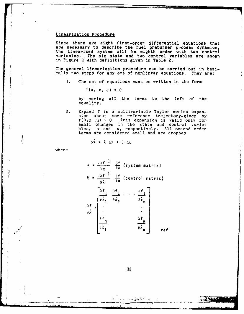
Linearization Procedure

Since there are eight first-order differential equations thatare necessary to describe the fuel preburner process dynamics,the linearized system will be eighth order with two controlvariables. The six state and two control variables are shownin Figure 3 with definitions given in Table 2.

The general linearization procedure can be carried out in basi-

cally two steps for any set of nonlinear equations. They are:

1. -The set of equations must be written in the form

f(x, x u) = 0

by moving all the terms to the left of theequality.

2. Expand f in a multivariable Taylor series expan-sion about some reference trajectory-given byf(O,x ,u) = 0. This expansion is valid only forsmall changes in the state and control varia-bles, x and u, respectively. All second orderterms are considered small and are dropped

SA = A Ax + B Au

where

A =- _df-1A(system matrix)

B = -' (control matrix)a u

af af af

9X1 x2 an

Lf

af af

1 n ref

32

- - -r-~--~-

LI)

LJ

-LJ A

3 03

X~ .4 -'

tt .aLA

ZVI = .4

S3

TABLE 2

SUMMARY OF SSME PERFORMANCE CONTROL REQUIREMENTSSTATE, CONTROL AND AUXILIARY

VARIABLE DEFINITIONS

NO. STATE DEFINITION

1 DWFPO - Fuel Preburner Oxidizer Flow Rate(lbm/s)

2 SF2 - High Pressure Fuel Turbopump Speed (RPM)

3 PMFVD - Main Fuel Valve Downstream Pressure(PSI)

4 DWFPF - Fuel Preburner Fuel Flow Rate (lbm/s)

5 DWFNBP - Primary Fuel Nozzle Bypass Flow Rate(lbm/s)

6 PC - Main Combustion Pressure (PSI)

CONTROL

7 FPOV - Fuel Preburner Oxidizer Valve Setting(3)

8 CCV - Coolant Control Valve Setting (%)

AUXILIARY

9 TFP - Fuel Preburner Temperature (OR)

'0

34

and

f ",. ax . •9 afn . . . f

;.af au eL9 i 3Xn refL

where fref means evaluated at the steady state operating point.

When applied to the sixth order model, the linear model becomes:

-2296.1 0 0 0 0 053.5 -25.0 0 -51.9 0 .081

0 0 -24.4 0 0 -32000.A = 0 0 0 -983.4 0 145.3

21826.7 0 0 -21173.7 7684.9 0

0 0 2. 0 0 261.4

F2.9xlO5 0

0 0B = 0 0

0 00 0 00 2.74xl0

1 where

AXT = ADWFPO, ASF2, APMFVD, ADWFPF, APC, ADWFNBP

= AFPOV, ACCV

function. For example, the frequency bandwidth for thrust mod-ulation will be significantly different than that for turbineinlet temperature spikes.

r5

i 35

Actuator Dynamics

For most purposes, it can be assumed that actuator dynamics donot influence the system or plant dynamics significantly. Thisis equivalent to saying that the actuator dynamics are restric-ted to high frequency (large eigenvalue) regions that implyfast response. In most instances, the actuator dynamics aresignificantly "faster" than the plant dynamics. This is nottrue for the SSME. The fuel preburner oxidizer valve and thecoolant control valve have open loop frequencies of -100 RAD/S,which is of the same order of magnitude as other system dyna-mics. Therefore, the actuator dynamics have been included inthe overall design process. The eigenvalues and the corres-ponding eigenvectors are shown in Table 3. As can be seen, theeigenvalue corresponding to the combustion pressure LPc(7684.09 RAD/S) is positive, which implies a nonminimum phasesituation. The smallest eigenvalue (-24.9 RAD/S) correspondsdirectly to LSF2, the fuel turbopump speed. The complex conju-gate pair of eigenvalues corresponds primarily to APMFVD, themain fuel valve discharge pressure. There is couplingbetween APc, ADWFPF, ODWFNBP, and APMFVD. The eigenvalue thatcorresponds to DWFPO, the oxidizer flow rate, is coupled to thecombustion temperature. The two actuator eigenvalues are loca-ted at -100 RAD/S. Mathematically, the control problem is tomove the nonminimum phase ( APc) eigenvalue to the left of thereal axis without triggering undamped oscillation of the oxi-dizer and fuel flow rates, which in turn causes the fuel pre-burner temperature to oscillate. The actuator dynamics can beapproximated as a first-order process with a time constant of10 Ms. For control Au(t) and input Ar(t), the differentialequation is

- T u(t) + 1Ar(t)

where T is the time constant.

The perturbation model for the fuel preburner oxidizer valve(AFPOV) and the coolant control valve (LCCV) is as follows:

d AFPOV(t [0 FPV(t)dt ACCV t ) T 1 ACCV(t)

0 AccvI(t)

36

r '

0000 0

41C.9 0 !co c 0 0 0

VC , C. C; C

1 0! 0Z a0 000 0

2 *0

0; ; -; C; C C; C

0 C0

ft o

to a-

o 0~ a @~t@'M 307

I

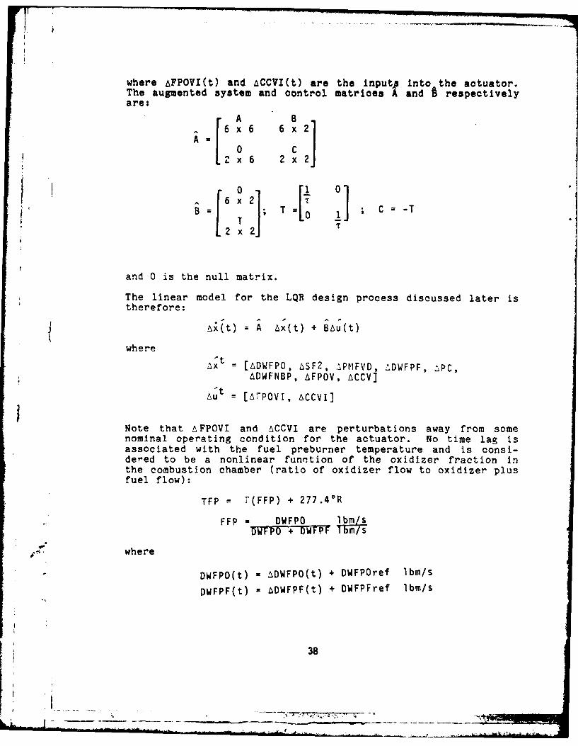
where FPOVI(t) and ACCVI(t) are the inputo into the actuator.The augmented system and control matrices A and B respectivelyare:

ABS x6c

6 x6 2 x

:I] ; C -TTL~1 TJand 0 is the null matrix.

The linear model for the LQR design process discussed later istherefore:

whee at) =A x(t) + BLutwhere

axt = [LDWFPO, LSF2, jPMFVD, .DWFPF, 2PC,

ADWFNBP, AFPOV, ACCV]

t: [=FPOVI, ACCVI]

Note that AFPOVI and ACCVI are perturbations away from somenominal operating condition for the actuator. No time lag isassociated with the fuel preburner temperature and is consi-de-ed to be a nonlinear funntion of the oxidizer fraction inthe combustion chamber (ratio of oxidizer flow to oxidizer plusfuel flow):

TFP = (FFP) + 277.4 0R

FFP = DWFPODWFPO "+ DWFPF Ibm/s

I., where

DWFPO(t) - ADWFPO(t) + DWFPOref Ibm/s

DWFPF(t) = ADWFPF(t) + DWFPFref Ibm/s

38

i __ ____

f . . . ..

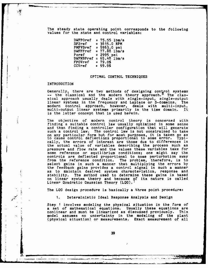
The steady state operating point corresponds to the followingvalues for the state and control variables:

DWFPOref = 75.55 ibm/sSF2ref = 3615.0 RPMPMFVDref = 5963.0 psiDWFPFref = 77.88 lbm/sPcref = 2995 psiDWFNBPref = 65.48 lbm/sFPOVref = 79.0%CCVref = 99.9%

OPTIMAL CONTROL TECHNIQUES

INTRODUCTION

Generally, there are two methods of designing control systems-- the classical and the modern theory approach. The clas-sical approach usually deals with single-input, single-outputlinear systems in the frequency and Laplace or S-domains. Themodern control approach, however, deals with multi-input,multi-output linear systems primarily in the time domain. Itis the latter concept that is used herein.

The objective of modern control theory is concerned withfinding a suitable control law usually optimized in some senseand then finding a controller configuration that will generatesuch a control law. The control law is not constrained to takeon any particular form but for most purposes, it is taken so asto cause control deflections proportional to some error. Typi-cally, the errors of interest are those due to differences inthe actual value of variables describing the process such aspressure and flow rate and the values these variables take forsome reference or equilibrium conditions; one might say the

controls are deflected proportional to some perturbation awayfrom the reference condition. The problem, therefore, is toselect gains in such a manner that multiplying the errors bythe feedback gains provides a control signal in such a manneras to maintain desired system characteristics, response andstability. The method used to determine these gains is basedon linear system theory and because ?f its nature is calledLinear Quadratic Gaussian Theory (LQG).

The LQG design procedure is basically a three point procedure:

1. Deterministic Ideal Response Analysis and Design

Step 1 involves modeling the physical situation In the form of

a set of mathematical equations. Usually these equations arenonlinear and must be lnearized as discussed previously. Thismodel assumes no uncertainty in the modeling of the plant(physical situation) or measurements. Exact measurement of all

39

I _ _i

L _ _.I .. . . . . . . ... . . . . ... . ... ... .

plant state and measurement variables is assumed. Actuator andplant dynamics are also assumed to be known exactly. The SSMEdeterministic model formulation describes the behavior of thefuel preburner state and measurement variables as well as theinteraction of the thrust (combustion pressure) with changes infuel preburner flow rates. The preburner temperature takenhere as an auxiliary variable, is assumed to be a nonlinearfunction of the oxidizer fraction in the combustion process andthe fuel temperature in the lines. For design purposes, thisnonlinear equation is used to calculate fuel preburner tempera-tures. The dynamics of the temperature are of such high fre-quency, that this dynamic effect can be ignored. The measure-ment or output variables will be the pressure and volumetricflow rate measured at the fuel flowmeter.

2. Stochastic Estimation Analysis and Design

Step 2 introduces uncertainty into the linear model to compen-sate for linearization errors as well as errors due to non-linear model uncertainty. Most plant variables in a realsystem cannot be directly measured by coj ventional techniques.Therefore, a state filter or observer9 ,O is used. Not onlyare plant variables assumed uncertain but sensor errors arealso assumed in error. These errors are described statis-tically by intensity matrices of covariance I0 .

3. Stochastic Feedback Control System Design

From Steps 1 and 2, an optimal control correction from theestimated state deviation (error) is derived. The controlleris then tested in the linear system to determine how good thecontrol gains are in meeting design goals.

In general, a control system is designed for each set oflinearized equations that describe the dynamics of the SSME inthe neighborhood of several equilibrium conditions. For thisparticular problem, the mixture ratio of 6:1 at rated powerlevel (RPL) is of interest and hence is used as the referencecondition about which to implement the controller design. Thetechnique for designing the control system is the previouslymentioned LQG theory, which provides a somewhat systematicmethod for determining a set of feedback gains. In most cases,the design for each steady state condition yields a set ofunique feedback gains. The resulting designs are then testedby observing the time responses to typical input commands. Inthis case, these commands consist of a step-type combustionpressure (thrust) or preburner fuel and oxidizer flow ratechanges.

40

NA-_

THE OPTIMAL REGULATOR

Introduction

For the SSME design point discussed previously dealing with theSSME hybrid model, a Linear Quadratic Regulator (LQR) design iscarried out that provides state feedback gains to the controlto minimize some cost function.11 The LQR controller alwaysprovides a control law that will drive perturbations or errorsfrom the ideal state and control variables to zero. It must beunderstood by the designer, however, that the LQR formulationdoes not allow constraints to be put on the control or statevariables. Such constraints, however, can be applied indirec-tly by the designer in the design process. In general, the LQRdesign procedure selects feedback gains in such a manner as tominimize the "cost" of the process in a rigid mathematicalsense.

In the following sections, the general formulation of the LQRdesign problem is presented. In addition, a procedure will bediscussed that will allow the designer to "constrain" selectedvariables in order to stay within the prescribed limits of theengine.

The Regulator Design As A Tracking Controller

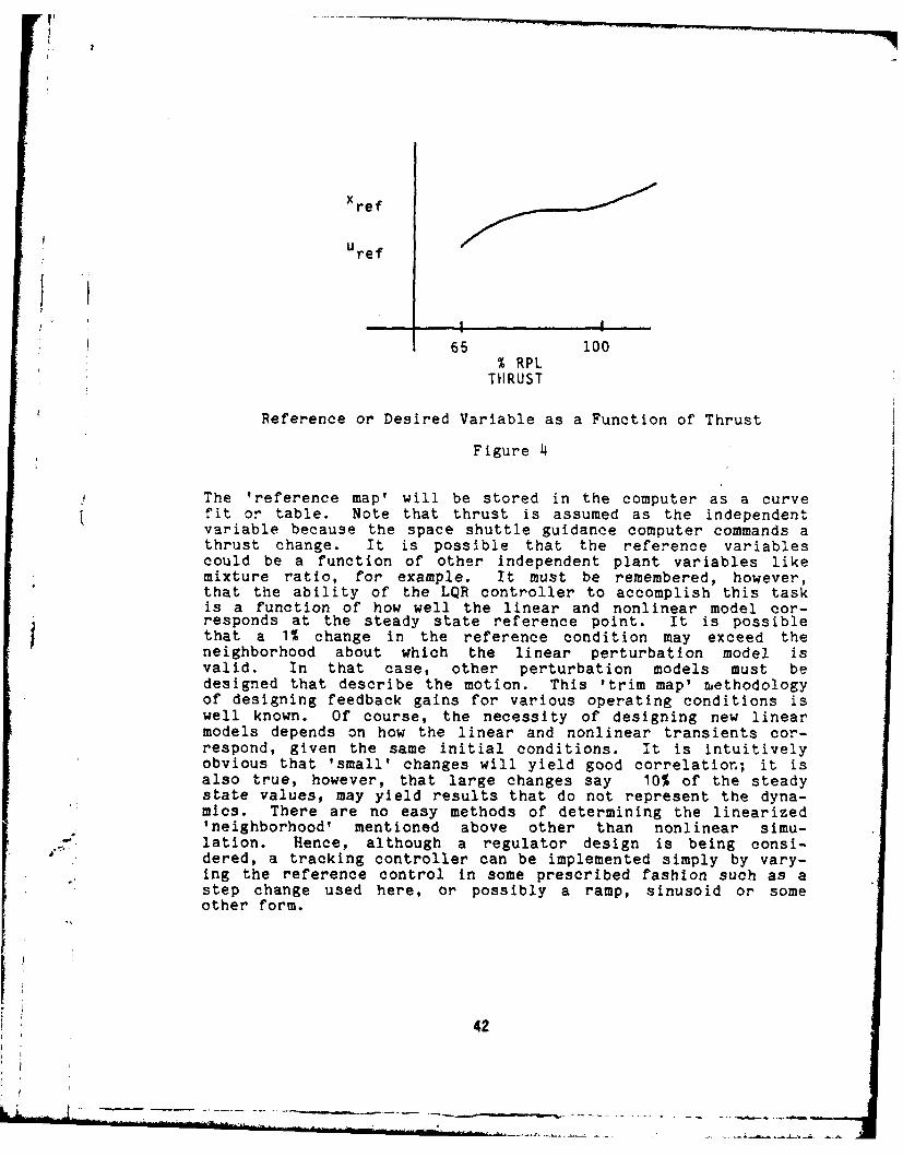
The LQR problem centers on designing a controller that keepserrors or perturbations small. However, the real problem ofinterest is that of carrying out step changes in the main com-bustion pressure, fuel and oxidizer flow rates in the fuel pre-burner in a reasonably short time while retaining good dynamiccharacteristics and at the same time not exceeding specifiedengine limits. Although these two problems appear different,they can be cast into the same form as will be shown. If theengine is operating at one steady state reference point and itis desired to change to another point, the regulator controlcan be used by simply changing the steady state referencepoint. Since the regulator tends to drive all errors to zero,it will drive the engine to the new operating point with newsteady state conditions. For example, suppose it is desired tochange the thrust level in 1% increments. For the variousthrust levels, there will be a unique set of steady state oper-ating conditions, as shown in Figure 4. This new set of steadystate operating points will then be substituted in place of theold reference points. The change in the variables in the sys-tem will then be driven to zero, and hence the engine will bedriven to the new operating point (new thrust level).

41

Xref

Uref

65 100% RPL

TiHRUST

Reference or Desired Variable as a Function of Thrust

Figure 4

The 'reference map' will be stored in the computer as a curvefit or table. Note that thrust is assumed as the independentvariable because the space shuttle guidance computer commands athrust change. It is possible that the reference variablescould be a function of other independent plant variables likemixture ratio, for example. It must be remembered, however,that the ability of the LQR controller to accomplish this taskis a function of how well the linear and nonlinear model cor-responds at the steady state reference point. It is possiblethat a 1% change in the reference condition may exceed theneighborhood about which the linear perturbation model isvalid. In that case, other perturbation models must bedesigned that describe the motion. This 'trim map' methodologyof designing feedback gains for various operating conditions iswell known. Of course, the necessity of designing new linearmodels depends on how the linear and nonlinear transients cor-respond, given the same initial conditions. It is intuitivelyobvious that 'small' changes will yield good correlation; it isalso true, however, that large changes say 10% of the steadystate values, may yield results that do not represent the dyna-mics. There are no easy methods of determining the linearized'neighborhood' mentioned above other than nonlinear simu-lation. Hence, although a regulator design is being consi-dered, a tracking controller can be implemented simply by vary-ing the reference control in some prescribed fashion such as astep change used here, or possibly a ramp, sinusoid or someother form.

42

k - . ----

Mathematical Formulation 11

Briefly stated, we wish to find a control law that will mini-mize a cost or penalty function.

J - . f- (AxTQ Ax + AUT R Au)dt (1)2 o

where Q> 0 and R >0 and hence drive perturbations in r and uto zero. This cost function is subject to the constraint thatthe variables Ax and Au must satisfy the differential equations

Ax = A Ax + B Au (2)

where A and B are constant system and control matrices,respectively. A quadratic cost functional as above is chosenbecause it penalizes large errors much more severely than smallerrors. As is clearly seen, the first term in Equation (1)penalizes errors in the state and the second term deviationsaway from the reference conditions for the control. There aretwo main reasons why Equation (1) is used. They are that it ismathematically tractable; that is, the theory has been wellestablished, and also that it leads to optimal linear feedbacksystems.

The solution to the problem of minimizing Equation (1) subjectto Equation (2) is given by a constant linear feedback matrix Kso that

Au(t) = -K Ax(t) (3)

where K = R'lBTS and S > 0 satisfies the steady state matrixRiccati equation.

-SA -ATS +SBR- BTS Q0

Existence of a unique positive definite solution to the LQRcontrol problem is guaranteed provided the nxmn "control-

*lability matrix"

[B:AB: .... : An-1B]

has rank n where n is the dimension of the A matrix and m isthe number of controls (columns in the B matrix).

Procedure

In general, the procedure for using the regulator method can bedivided into three main steps:

1. The Q and R weighting matrices must be selectedfor the cost functional. In Equation (1), notethat Q must be a -positive semi-definite matrixwhile R must be a positive definite matrix.

43

L I I I

2. The gain matrix K must be determined by solvingthe matrix Riccati equation (4) for the matrix Sand substituting the result in Equation (3).

3. The resulting control law must then be incor-porated into the original system and tested. Ingeneral, this step is carried out in two sub-steps. Initially, the controller design is triedin the linearized system for which it isdesigned, and if satisfactory characteristics areachieved, it is then tried in the original non-linear system. Most often, this controller veri-fication step is carried out using digital simu-lations of the linear and nonlinear systems on ahigh speed computer.

Although appearing straightforward, this procedure is not with-out some difficulties. In particular, problems can be encoun-tered selecting the elements of the weighting matrices in thecost function Q and R. Generally, only the diagonal elemen sare used with first guesses equal to approximately i/,where E is the maximum desired error in the variable associatedwith that term. Here then, is where the designer can initiateconsiderations for constraints on the state and control varia-bles; that is, they determine a "ball park" number for E. Mostlikely, however, step 3 reveals a dynamic response of the con-trolled or closed-loop system that is not that desired, andadjustments of the weights are necessary. Oftentimes, in orderto avoid unnecessary computer simulations of Step 3 as an aidto selection of Q and R weighting matrices, the ei~envaluesfrom the closed-loop system are used to determine various per-formance characteristics such as rise time, time-to-half ampli-tude, etc. If these characteristics are favorable, that is, ifthe closed-loop system response is "fast", then the systemresponse is simulated on a computer. If the closed-loop systemis "slow", then the weights are changed to achieve a fasterresponse. The fast and slow designations are related to therelative time it takes to achieve a steady state condition.

A method that proves to be successful in choosing the Q and Rweighting matrices is to change the diagonal terms one at atime and note changes in the closed-loop system characteristics(eigenvalues). Each new system is simulated on a computer togive an indication of how changing one element at a time in theQ and R matrices changes the closed-loop time responses.

r As mentioned earlier, the vehicle limits are not part of theLQR problem. They are, however, part of the overall designprocess. Because this system will be used as a tracking con-troller, some quick checks can be made to determine if the con-trols will exceed their prescribed limits for a given design.Since, for a step change in main combustion pressure (flowrates), all the states except for the biased variable will be

44

zero, the initial control deflections can be determined by mul-tiplying the feedback gain corresponding to the pressure changerequired by the desired change. The resulting control deflec-tion should be within the vehicle control limits. If the con-trol limit is exceeded, then the element corresponding to thecontrol in the R matrix is increased. This, in effect, pena-lizes the control.

In general, increasing diagonal elements in the Q and R ma-trices tends to penalize the variables corresponding to thoseelements. Therefore, in order to limit a state variable,increase the diagonal element in the Q matrix corresponding tothat state variable. In order to limit a control variable,increase the diagonal element in the R matrix corresponding tothat controlled variable.

This trial and error approach, augmented by the knowledge ofwhich errors are not important, all come into play when selec-ting weighting matrices. In any case, a regulator solution andhence, the corresponding feedback matrix yielding desirableclosed-loop system dynamics can be obtained with patience.

CONTROLLER DESIGN

INTRODUCTION

The Linear Quadratic Gaussian control scheme as discussed pre-viously is a relatively simple controller to implement in acomputer control system once the linearized models areobtained. For this paper, only the LQ regulator design metho-dology and implementation will be discussed. The addition ofthe Kalman-Bucy filter is not difficult and the overall"marriage" of the optimal state feedback with the Kalmaj-Bucyfilter can be found in any text on linear optimal control.

"2

The design point of 100% rated power level with the referenceconditions for the six states and two controls is used as adesign point to determine a feedback matrix, not necessarilythe only one, that will produce the desired behavior in theneighborhood of the design point. Ideally, one would like allthe feedback matrices found to be the same so that a constantgain system results. In most cases, however, the feedbackmatrices are different. Consequently, either some scheme mustbe incorporated into the controller that senses the engine'sstate and condition or some alternate scheme must be deve-loped. Although there are several variations of gain sche-duling techniques, most require some method of estimatingstates and parameters (Kalman-Bucy filter).

The LQ regulator gains are found from the commanded thrust,which is commanded by the space shuttle guidance computer.From simulation studies, a 'trim map' of state and control

45

variables as a function of thrust level can be used to 'trim'or drive the system to the new thrust level. For differentthrust levels, there will be a unique set of reference valuesfor the state and control variables. Theoretically, if thefull set of actual state and control values are at a referencecondition, the thrust level should be unique. Therefore, ifthe computer commanded a 1% change in thrust level from say 65%RPL, the computer would search a set of steady state or refer-ence state and control variables that are curve fitted or intable form for the commanded or desired values of these para-meters needed to drive the system to the new commanded thrustlevel. The feedback gains will then drive the system to thenew state and control, and hence to the commanded thrust level.

The LQ gains are found from a curve-fit or table lookup of thegains versus the thrust level. For small changes in thrustlevel, the gains should vary smoothly. Although there is noguarantee that this will occur, it has been found for vehiclecontrol that LQ gains will vary in a smooth manner if the stateand control weighing matrices do not need large adjustmentsfor good control.l 3

The LQ gains determined for the design poit model discussed inthis paper were found using ORACLS.1" This package iswell-known among the modern control community and will not bediscussed. The use of this package of routines, h6wever, isrecommended because of its simplicity in accessing variousmatrix manipulation and LQG design algorithms.

The following sections discuss the controller design for thefuel preburner linear system derived previously. A sectiondiscussing controller implementation as well as linear simula-tion results is included. Also, the effect of limiting thecontrol in the linear simulations is discussed.

LINEAR MODEL SELECTION

From past studies, it was determined that fourteen states andfive controls present in the SSME could be used to develop alinear model to describe the engine throughout the flight enve-lope. However, since the control objective was to control pre-burner temperatures, it was decided to concentrate on the fuelpreburner since thermal spikes there are more severe. Furthermodeling experience indicated that only nine state and threecontrol variables could have any dynamic effect on fuel pre-burner temperature. From an eigenstudy of the open-loop dyna-mics of the system, it was found that certain states had vir-tually no effect on preburner temperature because of the highfrequency character of their associated elgenvalues. It wasalso discovered that the associated eigenvector was dominatedby that state. Intuitively, this means that the particularstate at a high frequency equilibrates long before other varia-bles in the system. (This type of analysis can be thought of

46

as modal decomposition since the system matrix v-ielded norepeated eigenvalues and hence the Jordon matrix1 is Justthe matrix of eigenvalues.)

After eliminating the row and column in the system matrix, theelgenvalues and eigenvectors were calculated again. In thevariables deleted from the linear model representation, it wasfound that all high frequency dynamics were eliminated. It wasalso discovered that the states needed for the fuel preburnertemperatures did not have the same frequency level as the dele-ted states. The final linear system contained six state andtwo control variables. It was discovered later, however, thatthe actuator dynamics associated with the two controls were inthe same frequency range as the plant dynamics. Since there 's

no direct coupling between the actuator equations and the plantequations, the actuator poles were simply negative of theinverse of the actuator time constant (e.g., - ) taken as10 ms. The resulting eighth order system was used for the con-troller design model.

As previously discussed, the effectiveness of the control lawdepends primarily on how well the linear system represents thedynamics of the nonlinear system, since it is almost certainthat linear systems found from nonlinear simulations will beinaccurate due mainly to the fact that the nonlinear simula-tions cannot describe all dynamic variations. Also, since thelinear models are not of full-order, i.e., all the state andcontrols possible are not used, the linear control law derivedwill yield some steady-state error. Although this error shouldnot be severe, it might be advisable to include elements offurther compensation in the controller. The easiest method toimplement is to implement trim integrators on those statesexhibiting steady state error. This amounts to integrating thesteady state error over time and multiplying that by an inte-gral gain.SINGLE POINT LQR DESIGN

Since this study is a feasibility study into the applicabilityof the LQG technique toward preburner temperature control, onlyone reference or design point was chosen about which to derivea linear model. The typical design strategy for this designpoint linear system is to choose a set of Q and R weightingmatrices. Realistically, a real controller must incorporategains found for a 'trim map' of the engine operating range(e.g., varying thrust levels). For design points that arerelatively 'close' to one another, a 'middle' design point canbe used to determine a set of Q and R weighting matrices thatcan be used over the entire set of operating points to designcontrol laws. The LQR design for the one design point was car-ried out using the method described previously.The resultingoptimal design shows that a step change in Pc (main combustionpressure), which corresponds to a change in thrust level with

447

47

- . . . . . V ' J : +' : + ' + + .. . .. . .

all other deviations zero, resulted in good dynamic behaviorespecially as the model dynamics influence the fuel preburnertemperature. The linear system simulation run for a Pc chancefrom nominal of -10 psi for a time interval of 0 to .1 s isshown in Figure 5. For Pc changes greater than -10 psi, mul-tiple step changes could be made until the required step changeis made. From iterations on the Q and R diagonal weightingmatrices, a final set of gains was found using the weights

S1.01 1.010 1 1.0, 1.0, 1.0.10, 1.0101 3

The eigenvalues from the closed-loop system show considerableimprovement over those of the open-loop, as can be seen below:

EIGENVALUESOPEN-LOOP (s- 1) CLOSED-LOOP (s-1)

-24.9 -190.0-142.9 + 223.51 -951.0 + 130.01-142.9 - 223.5i -951.0 - 131.01-983.4 -1145.0 + 1285.01

-2296.1 -11 4 5 .0 - 1285.017684.9 -3323.0 + 3625.01-100.0 -3323.0 - 3625.01-100.0 -8266.5

The gains are:

AOWFPO ASF2 LPMFVD LDWFPP APCr

AFPOVI J -7.23 2.73 -8.04 10-6 7.86 -3.46

ACCVI 2.56 1.65 2.81 10- 2 -3.1 1.075

ADWFNBP AFPOV ACCV

.107 -204. .156

-1.59 156. -28.2 1

The improvement is mainly in speed of response since the elgen-values have been moved to _igher frequencies. The positiveopen-loop pole (7684.9 s') has been eliminated in theclosed-loop system. The closed-loop system elgenvalues showcomplex conjugate pairs. These elgenvalues, however, appear tobe well-damped, as can be seen in the simulation results. One

48

fr

VL

tC

aL

Id=

C)a 9

U

L .. O

(nJ

CLd

-3-

0c

ois Oil

( S W I 0 L Ua

49

cooud

a-a

0.50

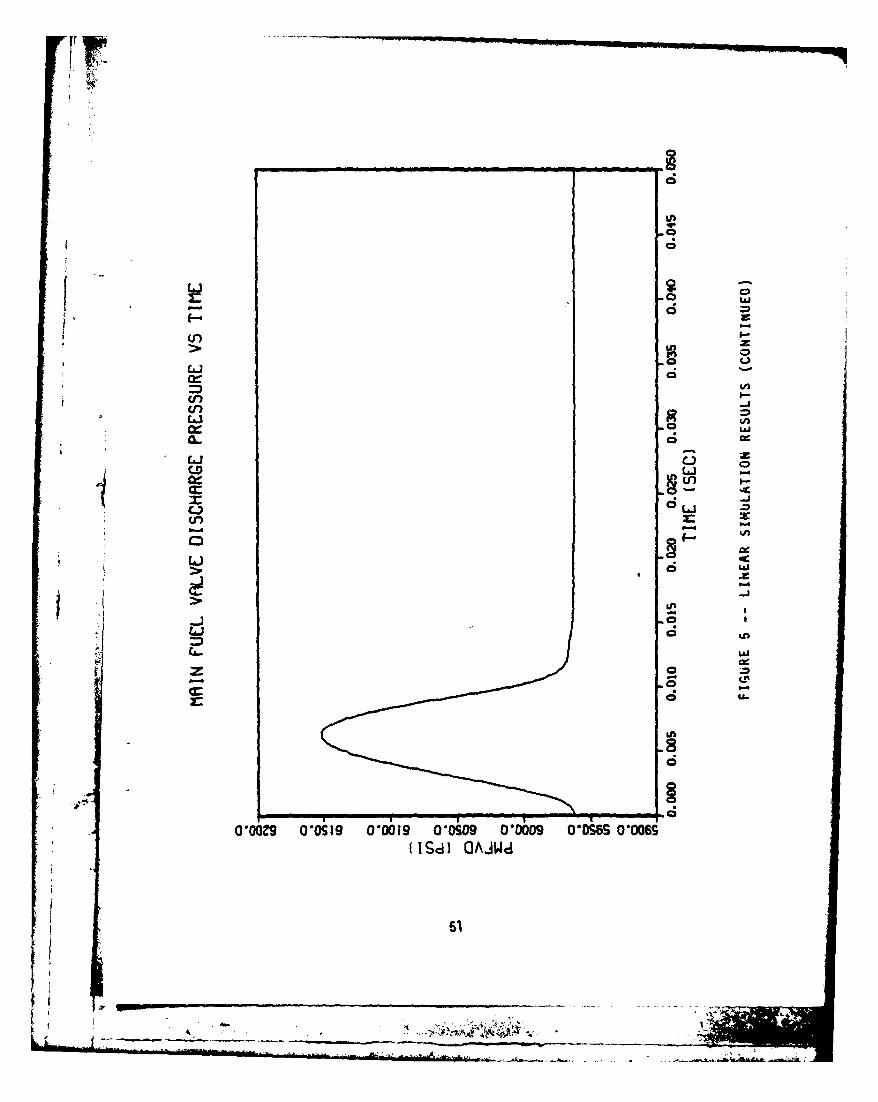
C

C$ a

Li gr a- df-S

'-4

(J*) I-z0

oLi -

aCr) I-U, -JLi

a ifl0~~

Li -% 2CD 0

I-

dLJ -JC-,

_ e-q -4

oLi

* LaJ-g-4

U,- Ia a

(dia U,

L.x

Z 0- -S

0

r C

.0

OOO~9 00S19 00019 00S09 00009 ODSBS 0006SUSd1 OAJWd

5'

.4-

LL~ A m-~-----~------- -* -

- ~ - - ~

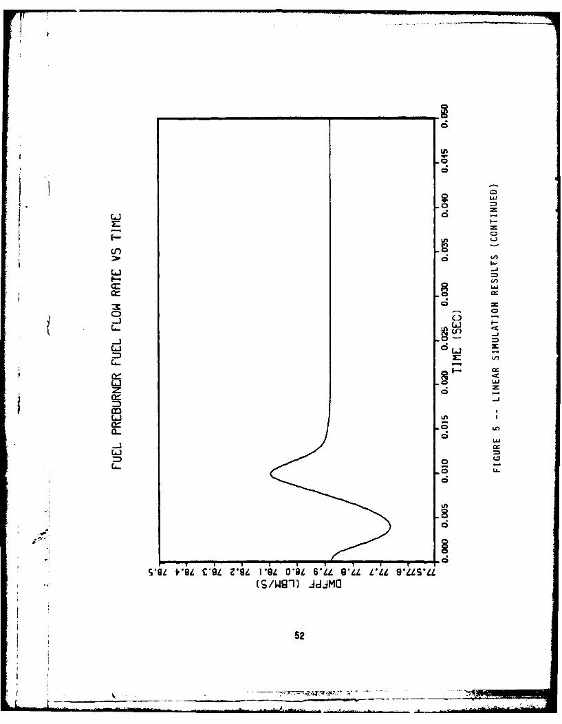
LLI

0 e

Li Li

z d

0C-

Li -h

0 - 0

VO V- i i ' ~L621 .LL2494i*(r,/Wgl JCJLi

K62 -

0mm

C3

LOA

I~I-

cz

-cc

cn-cc

a

L-

tnE

1%l5U

Ij It I ,c

53a

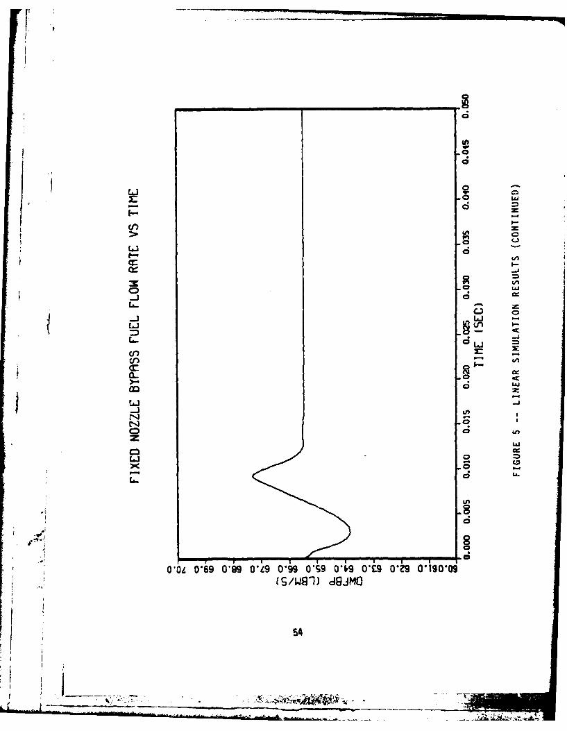
LLLJ

Z 0 wt-I-z

CC.)

cnn

Lo

0

C! ,

Lin

OIOL0*69019 OIZ 019 O'9 Ws WE OT 0010-0

54K

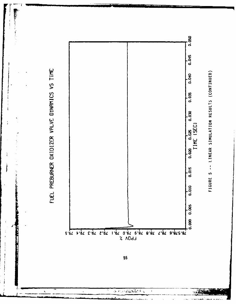
anm

c- 0

ci z1-J

00

z-J

CL

~U..

LIn

L--J

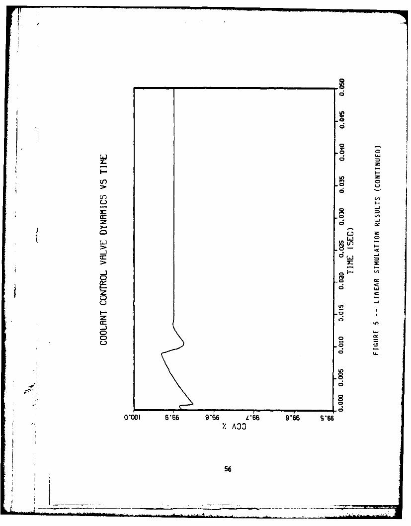
4.

(f))

C.)I-~ C

00z *L)

8

olo

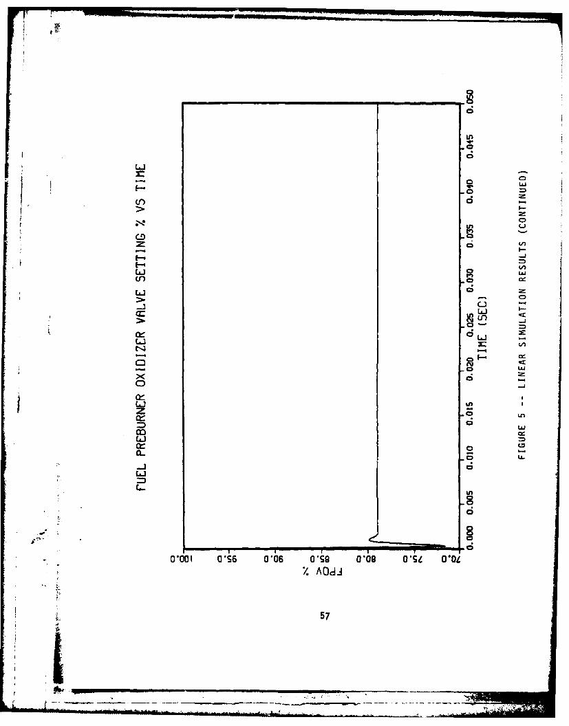
L6-

L63 CDC)

a. LI

EJV

z LO

CLC

Cl0

0100 OIS a 06 OS9 a69 -ii 0.0

AO0-*

57d U

WOM'~

V.90

0 -j

VCD

C-) C0W

L-

CD -

ca LO.

Li -

JS-

0 LL.

C) -J

0z0 0-609 *609 *6W '6060100A33,

58I

in

0 -

Ciir I-

Li -

cc

WdOM 01001 0 oo 106 ~

559

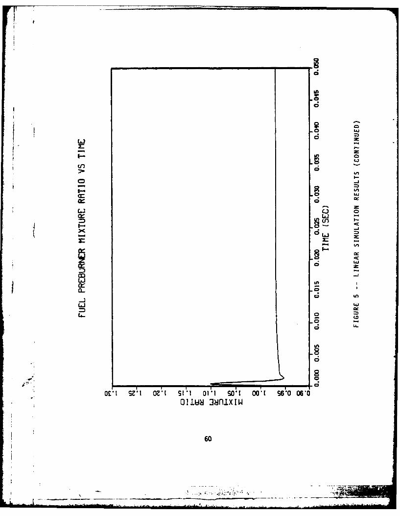
La

9

0--

o -Ju 3nx

60LI

of the major goals in this study is to control fuel preburnertemperature through oxidizer and fuel flow rate control. Sincefuel flow is difficult to regulate at this operating point(i.e., the coolant control valve is 99.9% open, which impliesmaximum fuel flow rate), fuel control will yield minimal effecton preburner temperature.

The actuator dynamics significantly affect closed-loopresponse, since commands from the feedback control law do nothave enough time to reach their steady state values before the

* next control command is input. A relatively large commandedchange in valve position will not be seen in the actuator dyna-mics response, since there is not enough time for the valve torespond (e.g., 10 ms time constant). This effect can be seendirectly by comparing the graphs of the fuel preburner oxidizerand coolant control valves setting commands with thecorresponding actuator response. For large perturbations, anonlinearity due to saturation of the valve limits the amountof valve movement that can be accomplished.

The maximum oxidizer flow rate amplitude is about 10 lbm/s,which shows up as a temperature increase of about 2000R.However, since the oxidizer flow rate changes damp out in about.03s, the preburner temperature also damps out as fast.

As the coolant control valve position is increased from 99.9%,the main fuel valve discharge pressure increases. However, theCCV limit of 100% full open causes saturation of the valve set-ting, which causes oscillation in the fuel flow rate. But,since the amplitude of the oscillation is about 0.5 lbm/s, theeffect on fuel preburner temperature is minimal. A small'ripple' can be seen in the temperature transient in the first10 ms. The commanded change in main combustion temperature of-10 psi is damped out in about 5 ms, although an overshoot of2 psi can be seen. The other transients associated with fuelflow rate, DWFNBP, DWFPF and SF2 damp out in 2 ms, the mixtureratio transient has settled in less than 2 ms.

Controller Implementation in the Nonlinear System

The feedback gains found earlier are designed using a linearsystem with constant coefficients. The variables which areinvolved with the linear system are error or perturbation vari-ables. Hence, the state error is multiplied by the gain matrixand the perturbation control is computed. In order to imple-ment this type of controller in an actual engine or in thiscase in the nonlinear engine model simulation, it is necessaryto convert actual variables into error or perturbed variables,apply the controller, then convert the perturbed control com-mands to actual control commands.

The feedback gains are implemented as in Figure 6. From thenonlinear system, the state variables x(t) are found. Thereference or steady state values, xn(t), are then subtractedfrom the current values to give the perturbed values Ax(t).

61

I,' N 7 *,. -- . ..

IVA

FIGUE 6 - FLW CHRT SOWIN LQRCONTROL LRILENTIOPROLE

62

The control law is then used to generate the perturbed controlvariables Au(t). This value is then added to the referencecontrol values, un(t), to give the actual control variableu(t) which is then limited to set actuator limits of 100%. Thefeedback matrix, K, is the LQR feedback matrix describedearlier.

CONCLUSIONS AND RECOMMENDATIONS FOR FURTHER STUDY

The following conclusions can be drawn regarding the feasi-bility of implementation of an LQR tracking control on the SSME.

1. The feasibility study was conducted with theassumption of perfect state knowledge. Measure-ments of some variables may not be available. Itis possible, however, to measure enough para-meters so that the system will be completelyobservable and hence a Kalman Filter or stochas-tic observer can be used to estimate systemparameters.

2. Linear models need to be designed at differentoperating points before any conclusions can bemade as to the control of preburner temperature,mixture ratio and thrust for different engineoperating conditions.

3. A linear model should be developed which includesboth the oxidizer and fuel preburners as well asthe main combustion chamber dynamics. A model ofthis sort will include the oxidizer flow dynamicswhich from this study affect preburner tempera-ture significantly.

This study has shown that preburner temperature control can beaccomplished using a simplified model of the preburner and theLinear Quadratic Regulator theory assuming full-state availa-bility for a typical main combustion pressure change. Furtherresearch in this control problem can be divided into the fol-lowing areas.

1. Low-order linear model derivation that wellrepresents the system dynamics at various opera-ting points. This model should include dynamicsrelevant to temperature control including thefuel and oxidizer preburners and turbines as wellas the thrust chamber dynamics. These models canbe derived through perturbation studies of a non-linear simulation model or by some piecewise ele-ments of the system and control matrices by com-* puter differentiation of the nonlinear equationevaluated at various operating conditions. Most

models generated by these methods are too large

63

* - * -

and do not contain the most convenient parameter-ization of the dynamics. Various methods can beused to derive this linear model the most attrac-tive of which involves modal decomposition whichsimply performs an elgenanalysis of thefull-state linearized digital SSME dynamicmodel. From eigenvalue and elgenvector studies,the matrix of eigenvalues should yield parti-tioned submatrices that will consist of high,middle, and low frequency dynamics. The highfrequency dynamics are assumed to be equilibrated(Aim=0) and hence reduce the model order. Somemiddle frequencies can probably be eliminatedfrom further study. It must be remembered, how-ever, that the partitioning of the system isdependent on the control designer's estimate ofthe frequency range of the control function. Forexample, the frequency bandwidth for thrust modu-lation will be significantly different than thatfor turbine inlet temperature dynamics. Actuatordynamics should also be included and realistictime delays built in to the simulation models forcontrol activity.

~. The set of low-order linearized models are thenused to design LQ-regulators.

3. A sensitivity study of the system should then beperformed to yield information concerning transi-ent changes due to varying system parameters suchas thrust for example. A sensitivity studyshould also yield clues to the type of gain sche-duling technique to be implemented.

4. A study should be perfor7-e that will develop aset of Kalman-Bucy filter ns (state estimator)assuming an observable system for each linearmodel. Gain scheduling techniques should also beinvestigated.

5. The Kalman-Bucy filters and their associatedLQ-regulator gains should then be tested on thelinear and nonlinear models for controller effec-tiveness over the flight envelope.

6. A feasibility study using performance resultmifrom above should then be performed to determineany hardware incompatibilities ignored in theabove steps. If the control designer has donehis Job correctly, a test program should beinvestigated to test the controller on a realengine.

64

This sequence is not meant to be all inclusive. Anychanges in this sequence will be a functinv if experienceas the control study progresses. This s, ,ence if fol-lowed should yield an excellent multivariaLim control lawfor the SSME that will significantly increase engineperformance.

i ACKNOWLEGEMENTS

The author wishes to express his thanks to S. Brandt forher patience and excellent typing ability. This papercould not have been completed without her. The authorwould also like to thank R. Brewster, R. Searle, E. Bekir,C. Landis and L. Sack for their technical assistance inmodeling and applying the LOR methodology to a very diffi-cult problem.

I If

.65

F

BIBLIOGRAPHY

1. Athans, M., "The Role and Use of the Stochastic Linear-Quadratic-Gaussian Problem in Control System Design.!- E..Transactions of Automatic Control, Vol. AC-16r~umbez 5,Dec. 1971

2. De Hoff, R. L., Hall, .-. ., "Design of a MultivariableController for an--Advanced Turbofan Engine," 1976 IEEEConference on Decision and Control, Clearwater BeachFlorida, Dec. 1976

3. De Hoff, R. L., Hall, W.E4 Jr., "Optimal Control of TurbineEngines," Journal of Dynamic Systems, Measurement, andControl, June 1979, Vol. 101

4. Taiwo, 0., "Design of Multivariable Controllers for anAdvanced Turbofan Engine by Zakian's Method of

* Inequalities," Journal of Dynamic Systems, Measurement, andControl, Dec 1979, Vol. 101

5. Merrill, W., "An Application of Modern Control Theory toJet Propulsion Systems," NASA Technical Memorandum, NASA TMX-71726, May 1975

6. Michael, G. and Farrar, F. (1973) "Development of OptimalControl Modes for Advanced Technology Propulsion Systems,"United Aircraft Research Laboratories (UARL) Report No.M9-11620-1

, 7. Nguyen, D. G., "Engine Balance and Dynamic Model," RockwellInternational Corporation, Rocketdyne Division, RLOO001,Rev. Ltr. G

8. Brogan, W. L., Modern Control Theory, Quantum Publishers,New York, 1974.

9. Luenberger, D. (1966) "Observers for MultivariableSystems," IEEE Transactions on Automatic Control, Vol.AC-i11.

10. Junkins, J. L, Mechanics: Dynamical Systems Introduction.i to Optimal E imation of Dynamic Systems, SiJthoff&~Noordhoff," 1975.

11. Bryson, A. E. and Ho, Y. C.: Applied Optimal Control, Ginnand Company, Waltham, Mass. 1969.

12, Kwakernaak, R., Sivan, R., Linear Optimal Control Systems,Wiley-Interscience, 1972.

66

i i_ _ _ _ _ _ _ _ _ _ _

13. Evatt, T. C., "Control Alternatives for an Unmanned FreeSwimming Submersible Vehicle", Master of Science Thesis,D-pt. of Aerospace and ocean Engineering, VPI & SU,August 1981.

14. Armstrong, E. S., Control and Systems Theory, Volume 10:

Marcel Dekker, Inc. 190.

* ~~~~~ ~ ~Nx p

RCSADsg ytmrrLn ae intltivar a lyleo tbl nk

0 1

* -

,

/

,

Next page Intentionally left blank.

* ' 6 7

VEHICLE SUSPENSION DYNAMIC OPTIMIZATION

Edward J. Haug4 Vlkram N. Sohoni

Sang S. KimHwal-G. Seong

Center for Computer Aided DesignThe University of Iowa

Next page intentionally left blank.

69

AD PO009 64VEHICLE SUSPENSION DYNAMIC OPTIMIZATION

Edward J. HaugVikram N. Sohoni

Sang S. KimHwal-G. Seong

Center for Computer Aided DesignCollege of EngineeringThe University of IowaIowa City, Iowa 52242

ABSTRACT

A vehicle suspension dynamic response design sensitivityanalysis and optimization technique is presented and illus-trated. Dynamic response measures included in the formulation,for use as the objective function or as constraints, includedriver absorbed power, driver peak acceleration, and suspensionelement travel. Design parameters available to the designerinclude suspension spring and damper characteristics, suspen-sion dimensions, and parameters in feedback control suspensionsubsystems. An adjoint variable technique that is generallyapplicable to such problems is employed and formulas for deriv-atives of dynamic response meas res with respect to designparameters are derived. Numerical results with a five degree-of-freedom vehicle model demonstrate feasibility of the methodand may serve as a guide for application to more complexmodels.

INTRODUCTION

V(ticle mobility modelling has progressed to the point thatperformance of actual or concept vehicles can be analyzed usingproven computer simulations. The NATO Reference Mobility Model(NRMM) [1] has been used extensively to evaluate vehicle ridequality and overall performance. It makes use of driverabsorbed power [2,3] as a criteria for determining maximumacceptable sustained vehicle speed over terrain and driveracceleration as a criteria for maximum acceptable vehicle speedover an obstacle. More recently, the Dynamic Analysis andDesign System (DADS) methodology has been used in detailedanalysis of vehicle dynamic response to gun firing, passageover terrain and obstacles, and weapon station stabilization(4,51.

To date, the mobility modelling methods noted above have beenused almost exclusively for evaluation of vehicles. Littleeffort has been devoted to extending these techniques as designtools. Methods of control system optimization [6] have been

71

_ _ _ _ _ _ _ _ _-_ _. . , •...

developed for mechanical system optimization [7], but have notyet been brought to bear on vehicle system design optimization.The purpose of this paper is to present and illustrate a methodthat can be used to build upon modelling methodology to obtaina design tool.

In order to be concrete in presentation of the method, a fivedegree-of-freedom vehicle model that is similar to idealiza-tions used in the NRMM is employed as an illustrative example.System equations are derived using Lagranges equations to yieldsecond order differential equations that depend on systemdesign parameters. These equations are then reduced to firstorder form, to allow easy development of design sensitivityequations. Absorbed power calculations, using a system offirst order differential equations, is then reviewed as a keyingredient in design problem formulation.

A vehicle design optimization formulation is presented tominimize driver absorbed power on a nominal road, subject tobounds on absorbed power on a rough road, driver peak accelera-tion over a discrete obstacle, suspension jounce and reboundtravel, wheel hop, and limits on design parameters. An adjointvariable method borrowed from optimal control theory [6] isthen derived for calculation of design derivatives of vehicledynamic response measures. An iterative optimization algorithm[8] is then outlined for vehicle design optimization. Its usefor solution of the five degree-of-freedom example is thenillustrated.

VEHICLE MODEL AND EXCITATION

The vehicle model used in this study is a five degree-of-free-dom (5-DOF) plane linear model shown in Fig. 1. The general-ized vehicle coordinates are the passenger seat displacementx1, the vehicle body vertical displacement x2 and rotation x3,and the front and rear wheel vertical displacements x4 and x5.The spring stiffnesses are denoted by k1 to k5 and dampingcoefficients are cI to c5 . Lengths are denoted by LI to L4 .The functions f1(t) and f2(t) represent displacements of thefront and rear wheels due to undulation in the road surface onwhich the vehicle is traveling.

The equations of motion for the vehicle are derived usingLagrange's equations of motion. In matrix form, they are

[M]X + (Chi + IKlx q(t) (1)

72

_ J

i4-

Kx

f tC x2

r i L

W 1(44L f(t

Figure 1. Five degree-of-freedom vehicle model

where

mI

/0I2

(M] m 3 (2)

0 min

L~m 5

where m3 is the pitch moment of inertia of mass m2 and

-C1 -L4 c1 0 0

(c1 +c2 +c3) (L4c I+L2c2-L3c3) -c2 -C3

[C] (L2c L 2 22L(4 1L 2+3c 3 ) -2c 2 L3c 3 3

.,: ::Symmetric (c2+4 0

•(c 3+c 5)

i 73

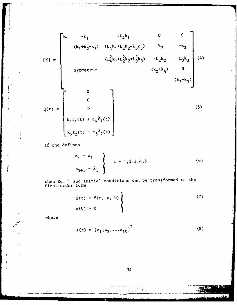
k1 k -4k 0 0

(k1 +k 2+k 3 (L 4 k1 L2 k2 -L 3k 3 ) -k 2 -

(K] -(L 2k +L 2k +L 2k) -L k2 L k3 (4)

Symmetric (k +k) 0

(k 3+k 5)

0

0

q~)0 (5)

k4 f 1 (t) + c4 t1(t)

k 5f2(t) + c5 2 (t)

If one defines

z =x

z.i =1,2,3,4,5 (6)

'5+i =

then Eq. 1 and initial conditions can be transformed to thefirst-order form

(t) = f(t, z, b) (7)

Z(0) - 0

where

z(t) [zlI1 9 2, ... Z 10]T (8)

74

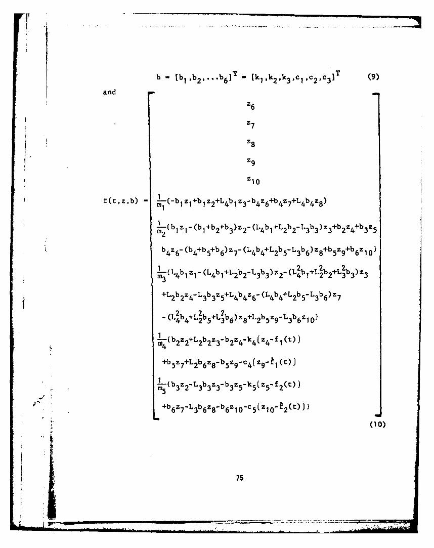
b -[b 1,b2 s**.b 6 IT [kl1 k 2 ,k 3 -cl-C 29 c3] (9)

and

z6

z 8

z9

z~o

f(tz,b) Lj-(-b z+b z+L b z3 b z +b~z+~~

L (b z -(b +b +b )z2-(L bl+L b -L b3)z+b z+b~M2

b 4 z6-(b4+tb5+b 6)z7-(L4b4+L 2b 5-L3b 6) z+b 5 z9 b 6 z10 1

1{ ( 4b1L2b- 2 2 2jj-Lb1 z-(Lb+~b-~ 3)z2-(L b +L bl+L'b3)z33412 3

+L2b 2Z4-L 3b 3 z5+L 4b4 Z6-(L 4b4+L~b 5-L 3b 6)Z7

2 2 2 )825 361

Li-b2 z 2+L 2b 2 z3-b2z4-k4(z4- f1 (t))"4

+b 5 z 7 +L 2 b 6 z8 -b 5 z 9 -c 4 ( z9 -t1 (t))J

1. (-b z -L b z -b z- k5(-f 2(t))

+b 6 ' 7 -L 3 b 6 z8 - b 6 z -c 5 (z 1 0 4t2 (t)) I

(10)

75

Numerical values of the model parameters used in this study aregiven in Table 1. The spring and damping coefficients givenfor the driver's seat and suspension will be the startingvalues for optimization.

Table 1. System Parameters

Index 1 2 3 4 5

Generalizedmasses m2 290 4500 41000 96.6 96.6(lb or l-in-sec2)

Spring coeff.k- 100 300 300 1500 1500

(lb/in.)

Damping coeff.ci 10 25 25 5 5

(lb-sec/in.)

Distance, Li 120 40 80 10(in)

In this vehicle model, the tires are modeled as pointfollowers, which are always in contact with the ground. If atensile force occurs between wheel and ground, wheel hop wouldactually occur. In the design formulation, a constraint pre-cluding wheel hop is imposed.

In vehicle dynamic response analysis, the input road conditionsare quite important. Dynamic response of the vehicle dependsstrongly on the vertical displacement history of the wheels onthe road surface. Typical road conditions are defined as asinusoidal undulation, with amplitude y0 and variable half-wavelength Ii. The front tire displacement v(y) at a locationy is defined as

yy[i 1] y i y y, i is odd

v(y) ="-1.1

y0[ i + cos,(yy yi- 4 y 4 y i is even1

-,**~ where y is a coordinate measured along the road and yi ,j-1

76

• , A.. ... .

If the constant speed of the vehicle is denoted bys, theelapsed time between front and rear tire encounter of the samepoint on the road surface is to - L1/s, where Li is thedistance between front and rear wheels. Then,

Y0 1 -cos wi(t-t)], tI f t 4 t , i is oddv(t) = (11)

Yo[1 + cos wi(t-t-) ti- I t f t , i is even

where wi ifs/l i and ti = yi/s. The vertical displacementfunction for the front wheel can therefore be defined as

v(t), 0 4 t T1 (

0 , otherwise

where T] is the time at which the road undulation ceases. Thevertical displacement of the rear wheel has the same value asthat of the front wheel, but with a time lag. That is,

f2(t) - f1(t-to) to T1 + t (13)

In this study, three different road profiles are used fordetermining the vertical displacement functions of the tires,as shown in Fig. 2. Profile (1) is a continuous sinusoidalcurve with a constant half-wavelength of 480 in. and anamplitude of yo ; 2 in. This profile represents a smooth high-way condition. Profile (2) is a continuous sinusoidal curvewith a constant half-wavelength of 60 in. and an amplitude of2 in., which represents a rough highway condition. Profile (3)is a combination of two sinusoidal curves with different half-wavelengths £i - 360 in. and £2 - 144 in. and an amplitude of5 in. This profile represents a severe bump condition.

The vehicle speeds for each road profile are as follows:

960 in/see (54.5 mile/h) for profile No. 1616 in/sec (35.0 mile/h) for profile No. 2450 in/sec (25.6 mile/h) for profile No. 3.

7?

• o

(a) profile no. 1

(b) profile no. 2

(c) profile no. 3

Figure 2. Road surface profiles

ABSORBED POWER

Absorbed power is a measure of the rate at which vibrationalenergy is absorbed by a human and is a quantity that may beused to determine human tolerance to vibration when a vehicleis negotiating rough terrain. The "absorbed power" concept wasdeveloped in the 1960's(2). although it has not been widelyused until recent years(l). In this study, the absorbed powerin the time domain is used as a measure of ride comfort.

Absorbed power equations given in the NATO Reference MobilityModel [1,2,3] are as follows:

p(t) " g(pz,b). 0 c t T

(14)p(O) - 0

where

p(t) [PIP2'' P7 ]T

78

S. ........... ......

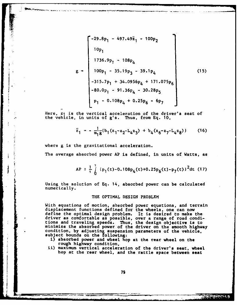
-29.8p, 497.49 1 - 10OP 2

lop1

1736.9p, - 108P4

g loop1 - 35 .19P 3 - 39.lP 4 (15)

-315.7p, + 34 .0956P4 + 171.075P6

-80.0pl - 9 1.36P4 - 30.28P5

pl - 0.108P 4 + 0.25P 6 - 6P7

Here, zl is the vertical acceleration of the driver's seat ofthe vehicle, in units of g's. Thus, from Eq. 10,

Z, F 1 -L + b}- (16)l jim b1 (zl z2-zL4z3 ) b4 (z6 -z7-L4 z8 ))

where g is the gravitational acceleration.

The average absorbed power AP is defined, in units of Watts, astTAP f (pl(t)-0.108P4(t)+O.25P6(t)-p 7 (t)l2dt (17)

0

Using the solution of Eq. 14, absorbed power can be calculated

numerically.

THE OPTIMAL DESIGN PROBLEM

With equations of motion, absorbed power equations, and terraindisplacement functions defined for the wheels, one can nowdefine the optimal design problem. It is desired to make thedriver as comfortable as possible, over a range of road condi-tions and traveling speeds. Thus, the design objective is tominimize the absorbed power of the driver on the smooth highwaycondition, by adjusting suspension parameters of the vehicle,subject bounds on the following:i) absorbed power and wheel hop at the rear wheel on the

rough highway condition,ii) maximum vertical acceleration of the driver's seat, wheel

hop at the rear wheel, and the rattle space between seat

79

and body, body and wheels, and wheels and ground on thebump road condition,

iii) design variables.

The optimal design problem may be written as follows:

Minimize *0" GIp1(t))dt (18)0

whereG(p) - {P1(t)-0.108P4 (t)+0.25P6 (t)-P 7(t)12 (19)

subject to the state equation of Eq. 7, the absorbed powerequation of Eq. 14, and the constraints

T 2*1 - f G[p 2 (t))dt - e1 < 0 (20)

02

*2 = Z f2(t) - 02 < 0, 0 < t < T (21)

*3 - "(z 5-f 2 (t)) - 03 < 0, 0 < t < T (22)

*4+( - 04 zL 0, 0t<c, (23)m 14 2 4mI 1+

*5 L (24)

*5 ' Iz 2 +L4 z 3 -z 1! 05 < O, 0 , t < T,

33 L 3*6 Iz 4 "z 2 "L2 z 3I - 06 0, 0 • t ' r, (25)

' 7 -2L 3z31 " 07 0, 0 < t 4 T, (26)

3* _ z-fl(t)l - e8 4 0 , 0 4 t < T, (27)

*9 -z3 (28)5 - f2(t) - 89 < O, 0 t 4 T

Ir *10 -(z35-f 2 (t)) - 010 0 O, 0 4 t < T (29)

where e, i - 1,2,...,10 are constraint bounds and zJ and pJare state and power solutions and j is the road profile number,defined as J-1 for the smooth highway, J-2 for the rough high-way, and j-3 for the bump, and the constraints of designbounds

80

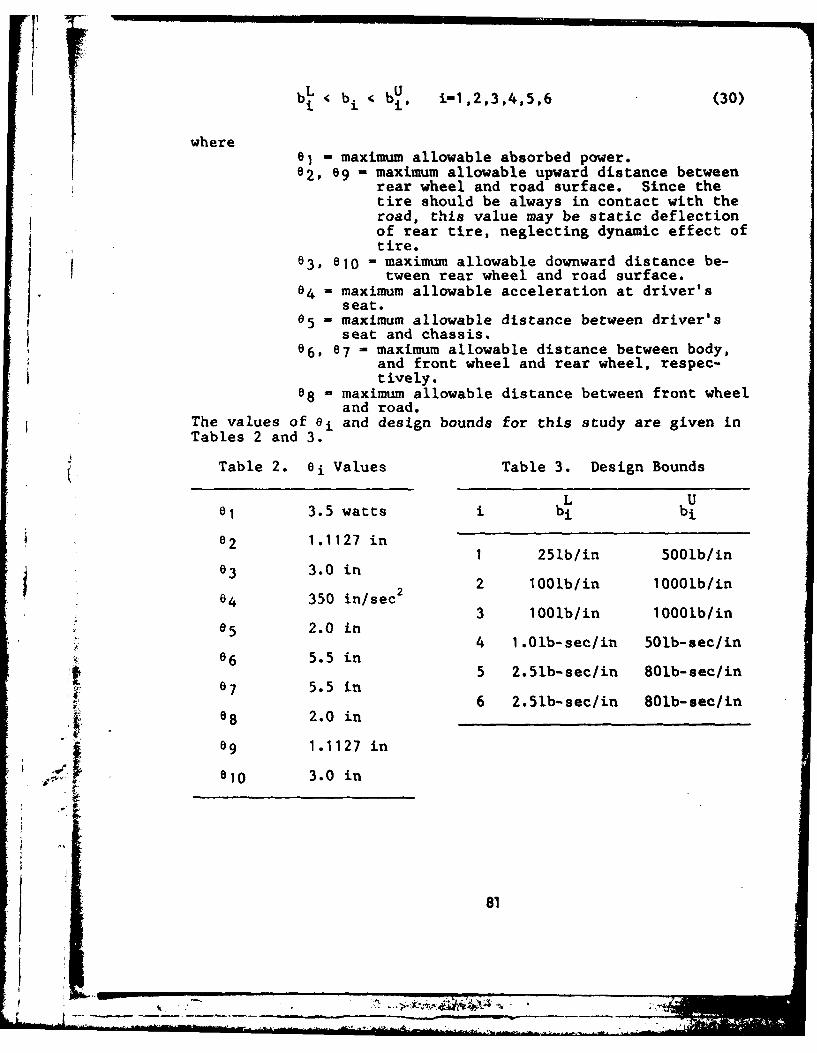
bL b biu , -1,2,3,4,5,6 (30)

where

e1 - maximum allowable absorbed power.

2 , 09 - maximum allowable upward distance betweenrear wheel and road surface. Since thetire should be always in contact with theroad, this value may be static deflectionof rear tire, neglecting dynamic effect oftire.

63, 010 - maximum allowable downward distance be-tween rear wheel and road surface.

4 - maximum allowable acceleration at driver'sseat.

65 - maximum allowable distance between driver'sseat and chassis.

e6, 67 - maximum allowable distance between body,and front wheel and rear wheel, respec-tively.

08 - maximum allowable distance between front wheeland road.

The values of ei and design bounds for this study are given inTables 2 and 3.

Table 2. oi Values Table 3. Design Bounds

L U01 3.5 watts i bi bi

6 2 1.1127 in1 25lb/in 5001b/in

e3 3.0 in

04 350 in/sec 2 2 1001b/in 10001b/in

3 100lb/in 1000lb/in8 5 2.0 in 4 1.01b-sec/in 501b-sec/in

06 5.5 in5 2.51b-sec/in 80b-sec/in

07 5.5 in6 2.5lb-sec/in 801b-sec/in

,8 2.0 in

89 1.1127 in

810 3.0 in

81

.. ~_1 _X~

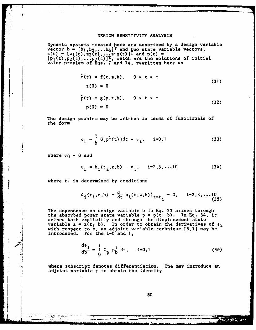
DESIGN SENSITIVITY ANALYSIS

Dynamic systems treated here are described by a design variablevector b - 1 b 2 , .. b6 ]T and two state variable vectors,zvet) tZ l(t),z2(t),...zlO(t)]T and p(t) -

[1p(t),P2(t),...p7(t)]T, which are the solutions of initialvalue problem of Eqs. 7 and 14, rewritten here as

1(t) - f(t,zb), 0 4 t c T(31)

z(O) - 0

p(t) - g(p,z,b), 0 4 t 4 (

p(O) =0

The design problem may be written in terms of functionals ofthe form

T

*i f=1 G(pi(t))dt - ei, i-O,1 (33)

where 80 - 0 and

i = hi(tizb) - ei' i-2,3,...10 (34)

where ti is determined by conditions

di(tizb) - hi(tzb)t = 0, i-2,3,...10t htti (35)

The dependence on design variable b in Eq. 33 arises throughthe absorbed power state variable p - p(t; b). In Eq. 34, it

Iarises both explicitly and through the displacement statevariable z - z(t; b). In order to obtain the derivatives of *iwith respect to b, an adjoint variable technique 16,7] may be

"* introduced. For the i-0 and 1,

d - G pb dt, i-0, (36)0 P

where subscript denotes differentiation. One may introduce anadjoint variable y to obtain the identity

82=1 _.__________-__________ ,. ... _________,- - ' " - - i : : , _

y [j-g~dt 0 (37)

Taking the derivative of Eq. 37 with respect to b, one has

T T~~pb gpPb" zzb"gb ld

0

Integrating the first term by parts gives

} [;T+.TgJpb + YTgzzb + YTgb dt0

- T (T)pb(T) - 0 (38)

since Pb(O) - 0 from Eq. 32.

4: Since Eq. 38 holds for any function y, a function y can bechosen to satisfy the following differential equation andterminal condition:

;i + gT,'! i +T Gp, 0 4 t 4 T

i-1,2 (39)Y( - 0

Equation 36 may thus be written, using Eq. 38, as

T~ iT i T ')t(- gb- gbz)dt i-0.1 (40)

0

Another adjoint variable X is introduced through the identity

-1

Ar Tijf]t -0 (41)

Taking the derivative of Eq. 41 and integrating by parts gives

83

-j -

*TXTf T TjJ+fz)zb + X fb dt -A(C)Z b(r) 0 (42)0

since zb(O) - 0. By the same reasoning as above, theadditional adjoint equation is obtainel as

ii + fTX 9 T 1, 0 4t 4T

i-1,2 (43)

A (T) -0

Thus, Eq. 40 becomes

di T ~T T-J (YIgb+A ifb )dt, 1inO,1 (40

For the second kind of functional, Eq. 34 gives

h. [ zb(ti)4 (ti)(ti)b]+hi +hi t b i-2.,...I0as Z b t (45)

*Differentiating Eq. 35 with respect to b, one obtains

[i ti +Qi Z (t )](tipb + "iz b(ti + "i 0 (46)

Since Eq. 35 is to determine ti, the coefficient Of (ti)bcannot be zero and one has

(ti) b H7 - +flj f(t.) zb(ti) a +a t (ti)

(47)

Substituting Eq. 47 into Eq. 45, one has

d*i- {h~ +0pZ a z~i + hi

z z b b (48)

84

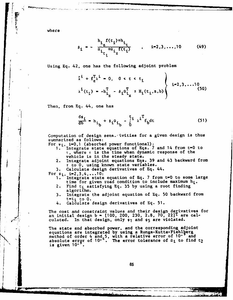
1. -.- . . ... ... ..... . . . . . . . . . .

where

hiz f(ti)+hit

2i 11z tj-i " ,i + f(ti) , i-2,3,...,10 (49)

Using Eq. 42, one has the following adjoint problem

1i + fTi _ 0, 0 t < t1 1-2,3, ...10

pin~ z (50)A (ti) -- h Hi(tizb)(

z z 1

Then, from Eq. 44, one has

d~i t 1T= + hi i+ 1 bfbdt (51)-

b b

0n i

Computation of design sensA vities for a given design is thussummarized as follows:For 4i, i-0,1 (absorbed power functional):

1. Integrate state equations of Eqs. 7 and 14 from t-0 toT, where T is the time when dynamic response of thevehicle is in the steady state.

2. Integrate adjoint equations Eqs. 39 and 43 backward fromT to 0, using known state variables.

3. Calculate design derivatives of Eq. 44.For *i, i-2,3,4,...10:

1. Integrate state equation of Eq. 7 from t-0 to some largetime for given road condition to include maximum hi.

2. Find ti satisfying Eq. 35 by using a root findingalgorithm.

3. Integrate the adjoint equation of Eq. 50 backward fromtmt i to 0.

4. Calculate design derivatives of Eq. 51.

The cost and constraint values and their design derivatives foran initial design b- [100, 200, 230, 2.8, 70, 22]T are cal-culated. In that design, only *1 and *5 are violated.

The state and absorbed power, and the corresponding adjointequations are integrated by using a Runge-Kutta-Fiehl ergmethod of order 4 and65, with a relative error of 10- andabsolute errgr of 10- 6 The error tolerance of 21 to find t2is given 10-

18

To check the validity of design derivatives, design.variationsare created by making a change of 5% in each design variable.Results for *0, *1, and *5 are given in Tables 4, 5, and 6.The predicted variations calculated by using design derivativesderived here show very good correspondence with the actualvariation, within 9% difference.

With design variation 6b - 0.05[bl,b 2 ,...b 6 ]T and multiplesbi - b0 + i6b, i-1,2,3,4, i.e., from 5% to 20% design varia-tion, the actual and predicted values of cost and constraintsare given in Figs. 3 to 13, where the solid line is actualIvalue and the dotted line is the predicted value. The pre-dicted values show good correspondence with actual values.

ITERATIVE OPTIMIZATION ALGORITHM

Many mathematical programming algorithms for solving optimiza-tion problems have been developed and evaluated for engineeringdesign optimization. In selecting an algorithm to be used, onemay base his choice on accuracy of the result, rate ofconvergence, time required for computing, computer storagerequired, and compatibility with engineering analysis methods.It is not possible, however, to order all algorithms in one andonly one way to say which is best. An algorithm may be poor asapplied to a certain class of problems, but effective inanother class. Hence it may be necessary to have a reserve ofalgorithms and to choose one, depending on the class ofproblems at hand. In this paper, the linearization method ofPshenichny [8] for optimal design of mechanical systems isused. This algorithm was originally presented in the Russianliterature, but has apparently only recently come to the atten-tion of workers in the west. Pshenichny has proved convergenceof the algorithm, using an active-set strategy that isessential in large scale mechanical optimization problems.

The general mathematical programming problem is to find b E Rnto minimize fo(b), with constraints

fi(b) 4 0, i-1,2,...,m'(52)

fi(b) - 0, i-m'+,...,m

where fi(b), i-0,1,...,m, are continuously differentiablefunctions. Note that fib) - 0 is equivalent to the in-equalities fi(b) 4 0, and -fi(b) < 0. Hence, one can limitconsiderations to the case with inequality constraints. Thus,one wishes to minimize fo(b), subject to the constraints

fi(b) 0 0, i-1,2,...,m (53)

86

............ ..................

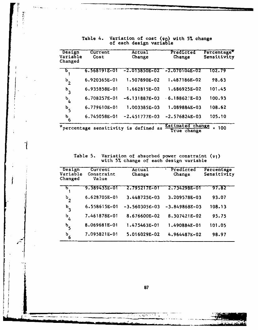
Table 4. Variation of cost (*0) with 5% changeof each design variable

Design Current Actual Predicted PercentagewVariable Cost Change Change SensitivityChanged

b 6.568191E-01 -2.013850E-02 -2.070104E-02 102.'791

b2 6.920365E-01 1.507890E-02 1.487186E-02 98.63

b 6.935858E-01 1.662815E-02 1.686925E-02 101.453b 6.708257E-01 -6.131887E-03 -6.188627E-03 100.934b 6.779610E-01 1.003385E-03 1.089884E-03 108.625b 6.745058E-01 -2.451777E-03 -2.576824E-03 105.106

*percentage sensitivity is defined aEstimated chanxe 100True change

ITable 5. Variation of absorbed power constraint (*1)

with 5% change of each design variable

Design Current Actual Predicted PercentageVariable Constraint Change Change SensitivityChanged Value

b 9.389435E-01 2.795217E-01 2.734298E-01 97.821

b 6.628705E-01 3.448725E-03 3.209578E-03 93.07, 2

b 6.558615E-01 -3.560305E-03 -3.849868E-03 108.133b 7.461878E-01 8.676600E-02 8.307421E-02 95.754

b 8.069681E-01 1.475463E-01 1.490884E-01 101.055

b 7.095821E-01 5.016029E-02 4.964487E-02 98.976

87

,AD-A126 966 PROCEEDINGS OF THE MEET ING 0F HEICOORDINATING GROUP 0ON 2MODERN CONTROL TH.U ARMY MAEREL SYSEMSARALYSISACTIVIT ABERDEEN PROVING GROG. H E COHEN JAR 83

UNCLASIE FG 4/ .N

1. i E 1

11111 L -

11111 ___ .6

MICROCOPY RESOLUTION TEST CHART14TIDNAI. BUREAU Of STANDARDS 1963-A

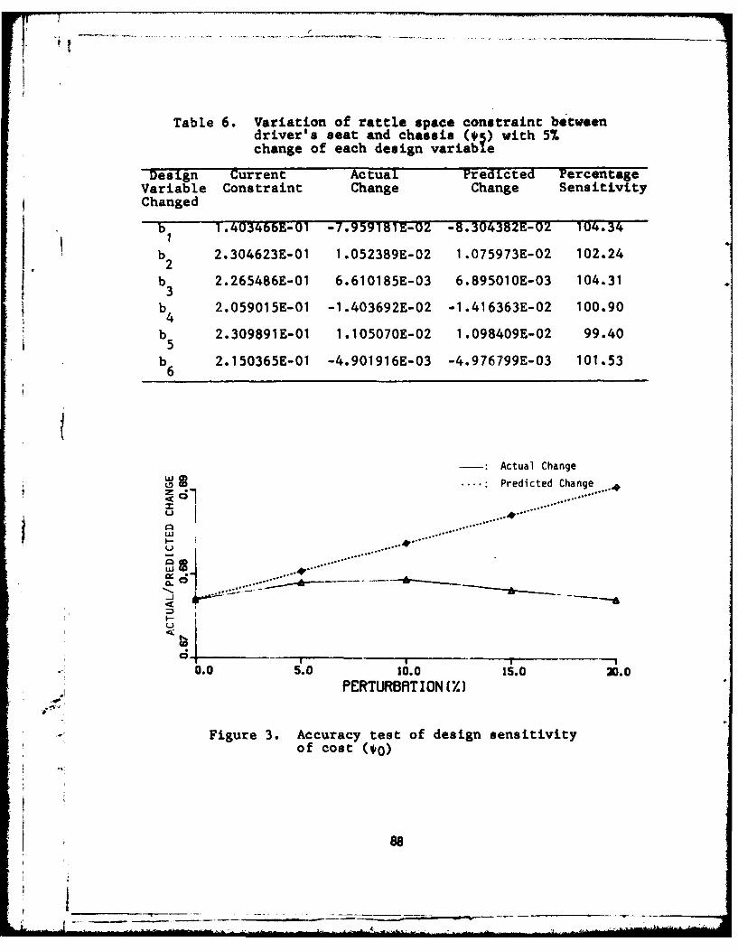
Table 6. Variation of rattle space constraint betweendriver's seat and chassis (5) with 5%change of each design variable

Design Current Actual Predicted PercentageVariable Constraint Change Change SensitivityChanged

b 1.403466E-01 -7.959181E-02 -8.304382E-02 104.34

b2 2.304623E-01 1.052389E-02 1.075973E-02 102.24

b3 2.265486E-01 6.610185E-03 6.895010E-03 104.31

b 2.059015E-01 -1.403692E-02 -1.416363E-02 100.904b 2.309891E-01 1.105070E-02 1.098409E-02 99.405b 2.150365E-01 -4.901916E-03 -4.976799E-03 101.53

-- : Actual Change

Predicted Change 4...............................

w ... ......

z C;

u.- . _ .... ....

0-.

0.0 5.0 10.0 15.0 20.0

PERTURBATION (%)

Figure 3. Accuracy test of design sensitivityof cost (*0)

~88

W ActualChange1 Predicted Change

*0.0 .016.0 15.0 20.0

Figue 4.Accuracy test of design sensitivity of absorbedpwrconstraint on rough highway (*1)

In -:Actual Change

* Predicted Change

LU

PERTURBAT ION M%

Figure 5. Accuracy teat of design sensitivity of rear wheelhop constraint on rough highway (02)

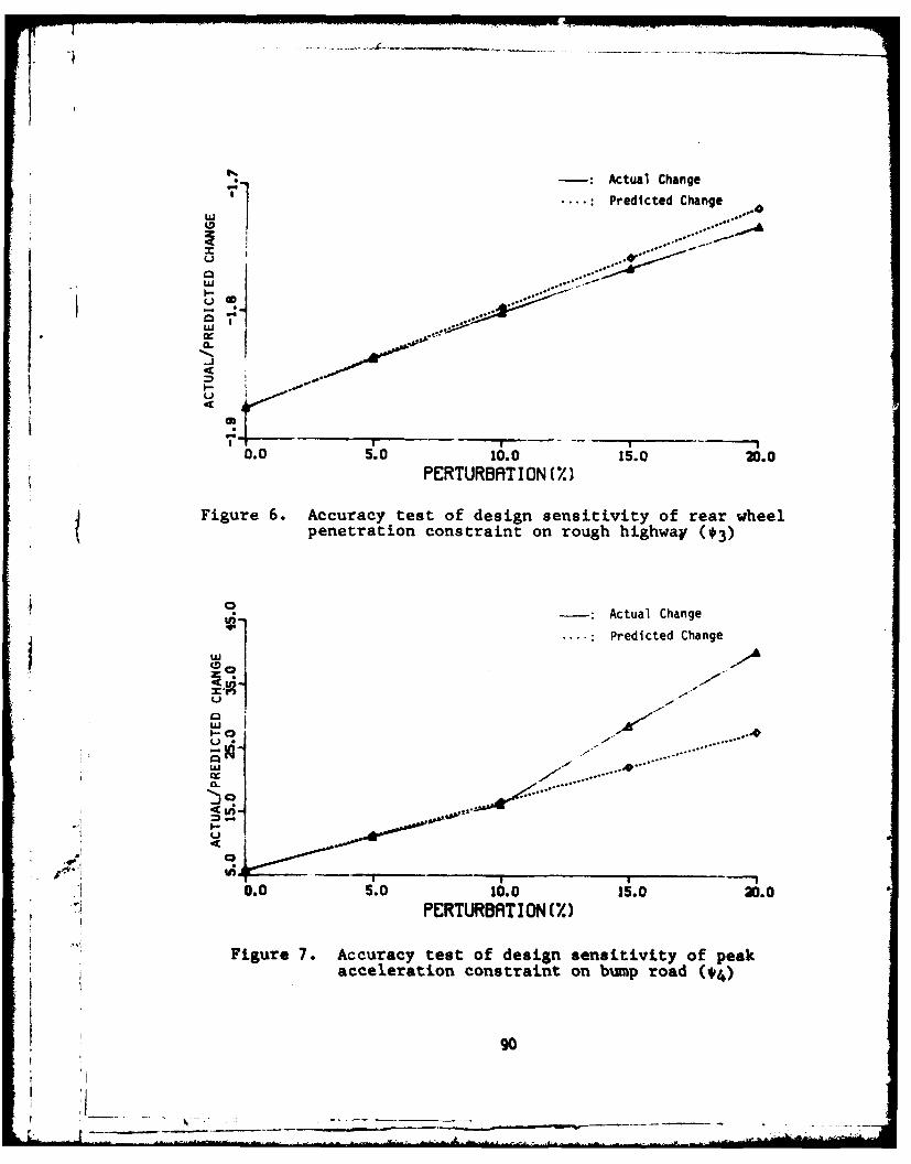
Actual Change

1 ... Predicted Change

ICL)

0o0 15.0 20.0

4 Figure 6. Accuracy test of design sensitivity of rear wheelpenetration constraint on rough highway (*3)

w I

9. Actual Change

...: Predicted Change

3

U

4Pf

.0 0 10.0 A.0 20.0JPERTURBAlTIONM%

Figure 7. Accuracy test of design sensitivity of peakacceleration constraint on bump road (*4)

90

L,- J.....

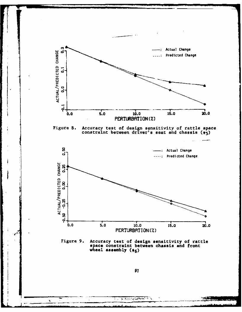
W Actual ChangePredicted Change

1.

...* . ..... . .............

0.0 5.0 10.0 15.0 20.0* PERTURBATION CX

Figure 8. Accuracy test of design sensitivity of rattle spaceconstraint between driver's seat and chassis (#5)

C-: Actual Change

* Predicted Change

C;)

* I

005.0 10.0 15.0 20.0PERTURBATIONMU.

Figure 9. Accuracy test of design sensitivity of rattlespace constraint between chassis and frontwheel assembly (06)

Actual ChangePredicted Change

U

* I I I5. 001502.

PETRATO X

Fiuet.Acrc eto dsg estvt frtlspc osrin ewe hassadrawhee aseml (7

I-

0.0 .0 0.0 5.020.0PERTURBATION (X

Figure 1. Accuracy test of design sensitivity of rtlraespace constraint between fisadrnt

wheel assembly androd )B

Predicte Change...--*

a ...... :Actual Change

Predicted Change

U)

U-.

0.0 S.0 10.015.0 2.PERTURBATIONM(.

4Figure 12. Accuracy test of design sensitivity of rear( wheel hop constraint on bump road (19)

Actual Change

... Predicted Changewj

IjJ

.4

0. 5.0 10.0 15.0 2.

PERTURBATIONM(.

Figure 13. Accuracy test of design sensitivity of rear wheelpenetration constraint on bump road (#10)

93

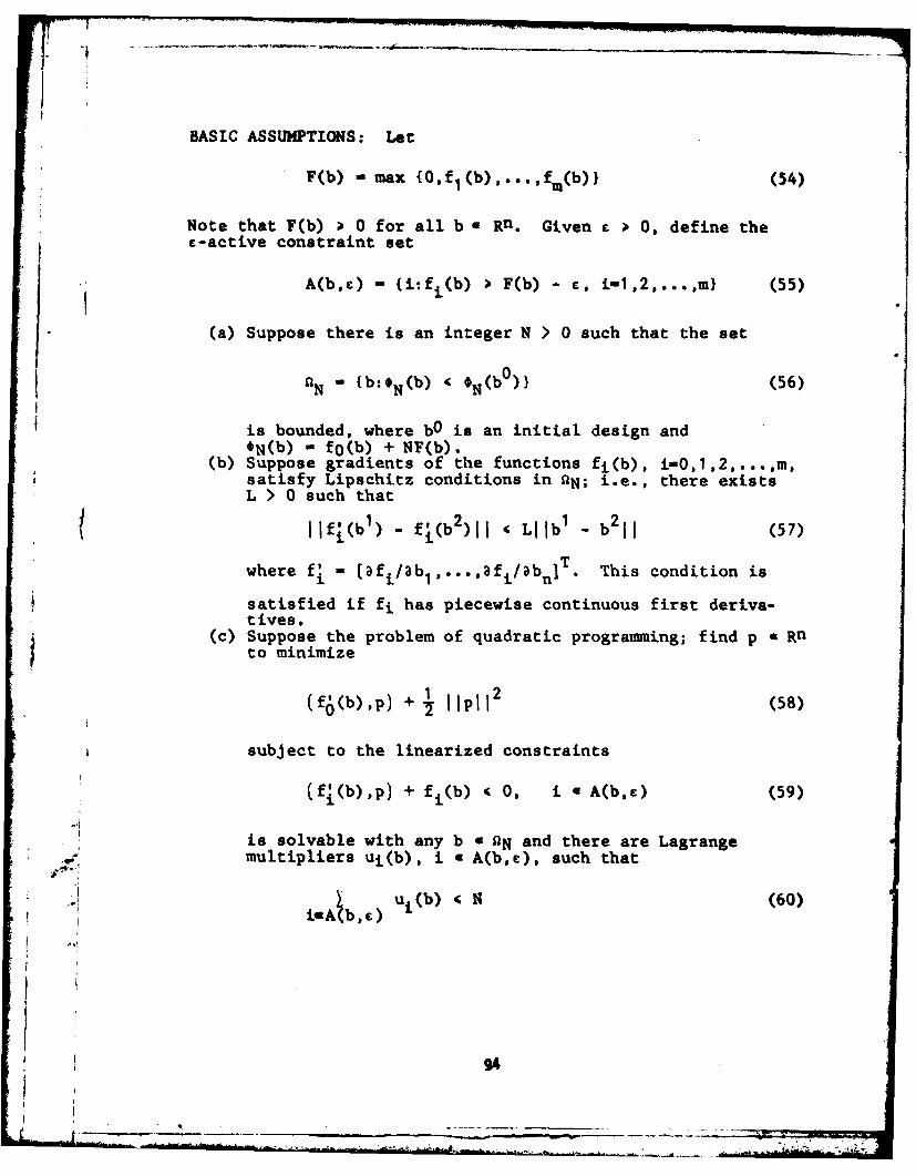
S- -. . -- " . .... . '.. .. . .

BASIC ASSUMPTIONS: Let

F(b) - max (O,fi(b) , . . . , fm(b)} (54)

Note that F(b) ) 0 for all b * Rn. Given c 0, define the

c-active constraint set

A(bc) - (i:fj(b) • F(b) - c, i-1,2,...,m) (55)

(a) Suppose there is an integer N > 0 such that the set

aN - {b:*N(b) ' *N(b 0 (56)

is bounded, where bO is an initial design and'N(b) - fo(b) + NF(b).

(b) Suppose gradients of the functions fi(b), i-0,1,2,...,m,satisfy Lipschitz conditions in ON; i.e., there existsL > 0 such that

Ilfl(b1 ) - fi(b 2 )1I e LI lb 1 - b2 11 (57)

where f- = [afi/abl,....afi/abn]T " This condition is

satisfied if fj has piecewise continuous first deriva-tives.

(c) Suppose the problem of quadratic programing; find p a Rnto minimize

(f6(b),p) + PH 2 (58)

subject to the linearized constraints

(fi(b),p) + fi(b) 4 0, i a A(b,E) (59)

is solvable with any b 4 ON and there are Lagrangemultipliers ui(b), i a A(b,E), such that

i'Ab,)ui(b) 4 N (60)ieA b,E)

-- . .. , . _ r - :, ; --- ---.. 94

i THEORETICAL ALGORITHM: Under the above hypotheses,.one may

state the following theoretical Linearizatton Algorithm of/ Pshenichny [8] :Let bU be an initial approximation and 0 < 6 < 1. For thekth iteration,(TY Solve the quadratic programming problem of Eqs. 58 and

59, with b - bk and solution pK - p(bk).(2) Find the smallest integer i such that

(bk + I pk) ( *(bk) _ 16 Pk1 2 (61)

2 2.

If this inequality is satisfied with i - i0 , let ek = 2

bk+1l bk + k

Under the basic assumptions, Pshenichny [8] has proved con-vergence criteria for the algorithm.

NUMERICAL ALGORITHM: The following numerical algorithm isintended for solving the problem of minimizing fo(b), subjectto the constraints of Eq. 52:Define

F(b) - max(0,f1(b),...,fm,(b), Ifm,+1(b)I ,...,fm(b)i)A(b,E) - {i:fi(b) o F(b) - e, i- 1,2, M

- (i: |fi(b)l -, F(b) - , i-m'+...,m)4N(b) - fo(b) + NF(b)

Select the initial approximation bO, No sufficiently large,co > 0, and 0 < 6 < 1.Step 1. In the kth iteration, solve the problem of finding uto miniml'ze

*(u) - 1f6(bk) + I uifi(bk)11 2 " ufi(bk)

k' k k kieA(b, c)uoB(b, e) i-EA(bk c)uB(b, E)

subject to ui ) 0, i A(bk,E), and ui arbitrary forafi afi

i a B(bk,e), where fj - *' n "

If the solution uk is such that #(uk) - -i, then setbk+1 - bk, ck+1 (1 /2 )Ek, and Nk+1 "Nk and return to Step 1.Otherwise, let

95

k "f0(bk) k ukif(bk) (62)k kixA(b ,C)uB(b ,C)

and go to Step 2.

Step 2. Set

bk+1 U bk + *kpk

k+1 k I

where ak is chosen equal to T and q0 is the smallest integer

for whichk (b k ) _k)kpkj112.N k (bk +q (b) --- 6k 2 q

k 2qk2

Step 3. If

kuki N k + IkI2 k~ Ui+ Ik li k Ik k ~ iI

iaA(bk ,) i.B(bk ,E) iA(b ,) iSB(bk c)

Then let Nk+1 - Nk. Otherwise, let

Nk+l = 2/ uk + I kjIieA(b, E) iaB(b,)

Step 4. If j jpk1 j is sufficiently small, terminate. Other-wise, return to Step I.

In implementing the algorithm, the derivatives fV are cal-i

culated using the adjoint variable method, which requires thatthe state and adjoint equations be solved forward and backwardin time, respectively. This is a substantial amount of com-putation that must be carried out during each optimizationiteration.

NUMERICAL RESULTS

Optimization of the vehicle suspension is carried out using thelinearization method. The initial design shown in Table 7 ischosen from Ref. 7. With the given initial design, the peak

96

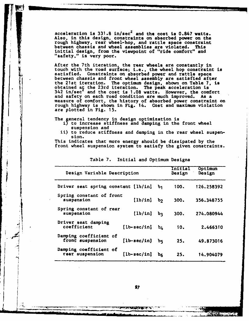
acceleration is 331.8 in/sec2 and the cost is 0.847 watts.Also, in this design, constraints on absorbed power on therough highway, rear wheel-hop, and rattle space constraintbetween chassis and wheel assemblies are violated. Thisinitial design, from the viewpoint of "ride comfort" and"safety," is very poor.

After the 7th iteration, the rear wheels are constantly intouch with the road surface; i.e., the wheel hop constraint issatisfied. Constraints on absorbed power and rattle spacebetween chassis and front wheel assembly are satisfied afterthe 21st iteration. The optimum design, shown on Table 7, isobtained ai the 23rd iteration. The peak acceleration is342 in/sec and the cost is 1.08 watts. However, the comfortand safety on each road condition are much improved. As ameasure of comfort, the history of absorbed power constraint onrough highway is shown in Fig. 14. Cost and maximum violationare plotted in Fig. 15.

The general tendency in design optimization isi)to increase stiffness and damping in the front wheel

suspension andii) to reduce stiffness and damping in the rear wheel suspen-

sion.This indicates that more energy should be dissipated by thefront wheel suspension system to satisfy the given constraints.

Table 7. Initial and Optimum Designs

Initial OptimumDesign Variable Description Design Design

Driver seat spring constant [lb/in] bj 100. 126.258392

Spring constant of frontsuspension [lb/in] b2 300. 356.348755

Spring constant of rearsuspension [lb/in] b3 300. 274.080944

Driver seat damping-j coefficient [lb-sec/in] b4 10. 2.466310

Damping coefficient offront suspension [lb-sec/in] b5 25. 49.873016

Damping coefficient of

rear suspension [lb-sec/in] b6 25. 14.904079

97 -- ----

00

CL

* Cz

00

0 .0 5.0 10.0 15.0 20.0

* ITERATION NUMBER

1Figure 14. History of absorbed power constraint (*I)

0

5. .0 10.0 15.0 20.0* ITERATION NLMIER

Figure 15. History of cost and maximum violation

CONCLUSION

The final results of the optimization, shown in Fig. 15 showthat the absorbed power over the smooth highway has beenincreased slightly, but that potential hazardous characteris-tics of the initial design have been brought under control byvirtually eliminating violations in constraints.

The success of the method for this simple dynamic system demon-strates the potential that exists in optimizing design for morecomplex and realistic systems. The computer optimizationmethod, using the adjoint variable technique has been demon-strated to be a useful tool in the design of vehicle suspen-

sion.

REFERENCES

1 Murphy, N.R. and Ahlvin, R.B. (1976), AMC-74 VehicleDynamics Module, Technical Report No. M-76-1, WaterwaysExperiment Station.

2 Pradko, F., Lee, R. and Kaluza, V. (1966), "Theory of HumanVibration Response," ASME paper.

3 Lins, W.F. (1972), Human Vibration Response Measurement,Technical Report No. 1151, US Army Tank-Automotive Command.

4 Haug, E.J., Jackson, G. and Beck, R. (1982), "Full ScaleSimulation of Large Scale Mechanical Systems," Proceedings,Fourth Meeting of the Coordinating Group on Modern ControlTheory, Oakland University, October, 1982.

5 Lance, G.M., Liang, C-G. and McCleary, M.A., "IntegratedSimulation of Vehicular Systems with Stabilization," Pro-ceedings, Fourth Meeting of the Coordinating Group on ModernControl Theory, Oakland University, October, 1982.

6 Bryson, A.E. and Ho, Y.C. (1975), Applied Optimal Control,Wiley-Halstead, New York.

7 Haug, E.J. and Arora, J.S. (1979), Applied Optimal Design,Wiley-Interscience, New York.

8 Choi, K.K., Haug, E.J., Hou, J.W. and Sohoni, V.N. (1982),"Pshenichny's Linearization Method for Mechanical System

* Optimization," Journal of Mechanical Design, to appear.

Next page Intentionally left blank.

99

....__ _ _....

COMPONENT MODE ANALYSIS OF LARGE SCALE INERTIAVARIANT MECHNAICAL SYSTEMS WITH FLEXIBLE

ELEMENTS AND CONTROL SYSTEMS

Ahmed A. Shabana and Roger A. WehageCenter for Computer Aided Design

The University of Iowa

Next page intentionally leftblank.

) |101

AD POO096 5COMPONENT MODE ANALYSIS OF LARGE SCALE INERTIA

VARIANT MECHAMICAL SYSTEMS WITH FLEXIBLEELEMENTS AND CONTROL SYSTEMS

Ahmed A. Shabana and Roger A. WehageCenter for Computer Aided Design

College of EngineeringThe University of IowaIowa City, Iowa 52242

t ! ABSTRACT

-A method is presented for transient dynamic analysis of mechan-.ical systems composed of interconnected rigid and flexible

bodies that undergo large angular displacements. Gross dis-placement of elastic bodies is represented by superpositionof local linear elastic deformation on nonlinear displacementof body reference coordinate systems. Flexible bodies are thusrepresented by combined sets of reference and local elasticvariables. Modal analysis and substructuring of the localelastic system is emploiyed to identify all modes and eliminatethe insignificant ones. Equations of motion and constraints

4are formulated in terms of a minimal set of modal and referencegeneralized coordinates, which are then dynamically adjusted toa time and inertia-variant eigenspectrum.

Control system differential equations are formulated andcoupled with mechanical system models. The composite nonlinearsystem of equations is then numerically integrated in the timedomain, to obtain complete system dynamic response. Exampleproblems are presented to demonstrate the algorithms and com-puter code. -------

1. INTRODUCTION

Dynamic analysis of large scale spatial nonlinear elasticmechanical and control systems require efficient numericalmethods. Modal techniques are desirable because they oftenallow reduction of problems with thousands of degrees of free-dom to manageable sizes. The main difficulty with analyzinginterconnected flexible mechanical systems, is that compositesystems are generally inertia-variant and their correspondingeigenspectrums are time dependent. This necessitates periodicre-evaluation of eigenvectors, an expensive process that shouldbe avoided.

To circumvent this problem, elastic properties of bodies arecharacterized locally, relative to body-fixed reference frames.When elastic displacements are small, which is often the case,they can be efficiently represented locally by modal analysis

103

.1

techniques because the local eigenspectrums are essentiallyconstant. Thus it is possible to efficiently reduce thedimension of a problem locally and then transform the muchsmaller problem to the global system and solve it usingexisting numerical methods.

The study of system flexibility has been a subject of majorinterest to many researchers. In the field of mechanics, therehave been a number of attempts to arrive at general algorithmsfor dynamic analysis of mechanisms with elastic links (1-11].However, most of these techniques assume that elastic deforma-tions do not significantly affect gross body motion. Inertiaforces of gross rigid body motion are first determined and thenintroduced as externally applied forces to the elastic model.In addition, most of these techniques are suitable for onlycertain classes of problems.

Some investigators [12-13] have solved simultaneously forcoupled gross body and elastic deformation. However, becauseof the highly nonlinear nature of these equations, these tech-niques have not utilized coordinate reduction techniques, norare they suitable for large scale systems.

A general method for dynamic analysis of large scale inertia-variant systems has been developed (14-15] which utilizes co-ordinate reduction techniques commonly employed in structuraldynamics and solves simultaneously for gross body motion andelastic deformation. The method in [14] is applied to largescalp control systems that contain elastic components. Mechan-ical systems are considered as collections of subsystems calledbodies, substructures or components.. Finite element or experi-mental methods can be used to characterize the elasticproperties of each deformable body. Energy equations of sub-elements are written separately and the elements of each body(substructure) are then assembled using a Boolean matrixapproach. The degrees of freedom of each body are then reducedusing a component mode technique. Adjacent substructures arethen interconnected using a Lagrange multiplier technique.Then a coordinate partitioning method [16] is employed toeliminate excess dependent equations of motion resilting fromimposition of the constraint equations.

2. GENERALIZED COORDINATES AND ENERGY EQUATIONS

In order to specify the configuration of a body or substructureit is necessary to define a set of generalized coordinates suchthat the global position and orientation of every infinitesimalvolume on the body is determined in terms of these generalizedcoordinates. As shown in Fig. 1 let the XYZ Cartesian coordi-nate system represent an inertial frame and the Xiy Z axesrepresent a Cartesian coordinate system rigidly attached tosome infinitesimal volume on the ith body. Using finiteelements, the ith body is divided into a number of rigidly

104

interconnected subelements. The location of an arbitraryinfinitesimal volume on the jth element of this body is definedin terms of two sets of generalized coordinates. The first setare reference coordinates locating the position of the body-fixed coordinate system relative to the inertial XYZ frame.The second set are elastic coordinates characterizing elasticdeformation of the body. Elastic coordinates represent rela-tive translational and angular displacement of infinitesimalvolumes at nodal points on the body. In addition the locationand angular orientation of every infinitesimal volume in eachelement can be approximated in terms of its elastic coordinatesand its shape function [17].

Let XijYijZij, as shown in Fig. 1, be a Cartesian coordinate

system with its origin affixed to an infinitesimal volume atsome point on the jth element of the ith body, that rotateswith this infinitesimal volume. The location of an arbitraryinfinitesimal volume, identified by the point piJ on thiselement, can be determined by specifying the position of XiYiZi

aid the location of the point p'J with respect to xiyizi. LetRI and and e' be rgspeqtively, the translational anf.rtaton-al coordinatEes of X'Y Z' with respect to XYZ... LS YJZIJ bea coordinate system parallel to the element X'3Y'JZ'J c99rdi-nate system and located at the origin of XiyiZiY Let e1J bethe nodal coordinates of the ijth element with respect toxijyijzij. 1t. ijdenote the location of point ph withrespect to XiJyiZ'J. The vector u J can be written as

7

ij ij -ij \u = e (1 X

where Oij is the shape functionof the ijth element,. Theposition of point p1J is specif-ied by

r =R + A' C'j *i0 iJeiJ / /

-(2)

where Ai(Oi) is th trtnsforma-tion matrTx from X1 YZ' to XYZ, XeiJ is the vector of elasticgeneralized coordinates of theith body defined relative to zXiyiZ i , and cij and tij are

transformation matrices from Figure 1. GeneralizedxijyijziJ to XiyiZi. Coordinates

If the rotation of XiJyiJZiJ with respect to XiYiZi is small,which is _be case for small elastic deformation, the matricesCi.] and C-J are approximately constant and Eq. 2 becomes

105

rJ Ri + A' NiJ eij (3)

where NiJ(xij, yiJ, ziJ) is the modified shape function of theijth element given by

Nij . cij *ij i1ij (4)

The kinetic energy of the ijth element is obtained fro thevelocity vector of the infinitesimal volume at point pTJ on theelement as

iJ = + A' NiJ eiJ + A' NiJ ;ij (5)

I.Pwhere (.) denotes differentiation with respect to time. Thesecond term of Eq. 5 can be expressed as

A N'J eiJ = BiJ (eieii)_i (6)

in order to isolate the velocity terms. Equation 5 is thenexpressed as

-ij = [I B ij A'Nij ] [A]iT 61 T ij ]T (7)T T (7

where I is an identity matrix. The kinetic energy o the ijthelement is obtained by integrating over the volume VI

TiJ . I f ij i T pJ dVij (8)

vii -P -p

where the mass density of the ijth element at piJ is pij andthe superscript T implies transpose of a matrix. Using vector

notation ji [_ _ _T and substituting Eq. 7 into

Eq. 8, kinetic energy becomes

Tij 1 iijT

106

4w

where MIJ , the mass matrix of the ijth element, is

M iJ P f ij B iJ T Bij TB iJ B ijT ANJ dV'J

V ij ij TT iT iT..LNJTA Ni1 AT BiJ NT N'3

(10)

The submatrix NiJ' N' associated with element elastic general-

ized coordinates is constant (see Eqs. 1 and 4).

Kinetic energy Ti of the ith body is obtained by summing ovfreach of its elements. Denoting the number of elements by n'

i

i = Ti (11)

j=1qilT i T qi i T T

In vector notation .i q [ , ,i2 in T

_q ii iq _qlM =diag (Mi I , M12, ..., M i n ), and Eq. 11 becomes

R i T -~i *i 12

The vector q is partitioned as

* *T T TA - r[ar (13)

r TT

where - [Ri, e are reference coordinates locatingei I- T ei 2 T, eiT T

xiyiz i relative to XYZ and . [e , e ... , e ] are

elastic generalized coordinates of the ith body.

Since Yis defined relative to x~izi a constant Boolean

matrix can be employed to impose constraints between adjacentelements on the ith body. These constraints in matrix form

j[ are

107

lip,_ _ - -- .---

- B: _q (14)

Differentiating Eq. 14 with respect to time and substitutinginto Eq. 12 yields

Ti 1 iTii (15)

where

Mi = BI i B (16)1 1

The kinetic energy of the ith body can be partitioned as

Ti 1t[r(--) i] r r (17)

where subscripts r and f denote reference and flexible coordi-

nates respectively. Observe that m is a constant matrix andff

also that coupling between elastic and reference coordinatesi i

exists through the nonlinear matrices mfi and tmr. Elastic andfr rf*

reference coordinates can be dynamically decoupled by neglect-ii

ing these two matrices and the dependence of B on elastic1

coordinates.

Strain energy of the ijth elastic element is given by [17]

U - f _kijTo i j dVi J (18)Vij

where ciJ and yiJ are the respective strain and stress com-" :ponenti at the-infinitesimal volume. The stress-strain

equation is given by the elastic constitutive relation

108

4________________

Oi j =GiJ3i j (19)

and the strain-displacement relation can be expressed as

EiJ = DiJuij

- DiJNi je i J (20)

where Dij is a differential operator relating strains and dis-

placements. Substituting Eqs. 19 and 20 into Eq. 18 yields

uij =1 e.. J ID.JN i GiJDiJNiJeiJdViJT

13

e _j ie' j (21)

where Kij is the ijth element stiffness matrix. The element

stiffness matrix is constant and the strain energy expression

is independent of reference coordinates because elastic

generalized coordinates are defined with respect to XiYizi.

The total strain energy of the ith body is

.TUi -T i -

U 1 [0Ri i

T qf ff qf

T iif] (22)f o f] f

ii

where Rff = diag 4ff, ff. .i

Substituting Eq. 14 into Eq. 22 and partitioning gives

.T 0 Of r

Y i T {0 (23)

109

i iiwhere _r and _f are as defined before and K is the stiffness

ffmatrix associated with the ith body elastic coordinates.

Finally virtual work of the ijth element is

aWi j - qijT6aiJ (24)

where -iJ is the vector of generalized forces associated withthe generalized coordinates _ . All forces except wgsklessconstraint forces between elements are included in SW-J. Thevirtual work of the ith body is

swi= iT iT .T T (25

i iwhere r and are respectively generalized forces associated

r fwith reference and elastic generalized coordinates.

3. SUBSTRUCTURE SYSTEM EQUATIONS OF MOTION

The composite vector of all system generalized coordinates isiT' 2T ,TT

designated as _ = a a2 ,... ,N , where N is the total

number of bodies (substructures) in the system. Nonlinearconstraint equations between adjacent substructures can bewritten in vector form as

±(_, t) - 0 (26)

where 0(_, t) - [41( , t),... ,m(S, t)IT and all equations areassumeJ to be independent. The equations of motion of the ithsubstructure can be written as [18].

d (Ti T _ (Ti )T + (Ui T - qi + OT i 0(27)

aa a aq

b where X is the vector of Lagrange multipliers.

Recall that all elastic deformation in the ith body is definedrelative to the body reference frame attached to node L whichimplies no elastic displacement at node 1. Thus

110

qf - 0 (28)

where i is the vector of elastic generalized coordinates ata~ft ]

i iT i T Tnode L. Denoting - If ,where p2_ is the set of

elastic generalized coordinates of the ith body excluding nodeX, Eq. 27 reduces to

ii)?+ 1 , t) + Piii) -

(29)

which is the general fo m of the equations of motion for theith body. The vector FT absorbs quadratic velocity terms ofEq. 27. These equations along with Eq. 26 form the constrainedequations of motion of the substructure. A coordinate reduc-tion technique is now employed to eliminate insignificantelastic degrees of freedom.

4. COORDINATE REDUCTION

Efficient solution of the system equations of motion requires atransformation from the space of system nodal elastic general-ized coordinates to the space of system modal generalized co-ordinates with lower dimension. This transformation is a con-stant mapping (19]. The problem is complicated by a timevariant system transfer function which implies that monitoringthe frequency content of external forcing functions alone isusually riot sufficient for predicting mode excitation becausethe mass matrix depends on generalized coordinates. Accord-ingly, no judgement can be made beforehand of the number ofsignificant modes to be retained for an accurate solution.

The method developed here is based on solving the eigenvalueproblem of the substructure once. From Fourier analysis of theforcing functions, an initial estimate of the number of modesto be retained is made, and during the simulation additionalelgenvectors are recalled or deleted as required. For thepurpose of determining eigenvalues and eigenvectors, if a sub-structure is assumed to vibrate freely about a reference con-figuration, Eq. 29 yields

ffflf + ffif -2 (30)

111

iwhere mi and k re the respective mass and stiffnessff f

matrices associated with the elastic coordinates. The stiff-

ness matrix 1i is positive definite because the reference co-ff

ordinate system is fixed. Equation 30 yields a set of eigen-vectors and a modal matrix. A coordinate transformation fromthe physical elastic coordinates to the modal coordinates isobtained by

Bi i i (31)f B2 A

iwhere BI is the modal matrix consisting of the eigenvectors2

obtained from Eq. 30, and i is a vector containing the modalcoordinates. Using Eq. 31 the reference and elast c general-ized coordinates are written in terms of the reference andmodal coordinates as follows

Pr00, [0 ir~ (32)

Li B 2 i)

Substitutin Eq. 32 into Eq. 29 and premultiplying by thetranspose o the matrix in Eq. 32 yields

i -i Ai T(2 )2 -P (2 , , t) -±i (2, t). (33)

R

The constraint Jacobian matrix of Eq. 33 is evaluated in termsof physical coordinates and converted to modal coordinatesusing Eq. 32 as

.Vi

[I Oi0(4-2 (P 0 B22

112

u~~~~~~ .... MN~-- ..

Equation 33 represents the reduced system of equations for theith substructure. The number of equations in Eq. 33 depends onthe number of elastic degrees of freedom required to achievethe desired accuracy.

5. CHARACTERIZATION OF PLANAR ELASTIC SYSTEMS

Figure 2 illustrates a typical jth element denoted as iJth oi.the ith body. The element X 13 axis is located at an angle OyJ

relative to the body-fixed Xi coordinate axis. The referencecoyrdiiates for this body are the tranglational variables(x, y') and the rotational variable e1 . This set of coordi-nats defines the position of the body-fixed coordinate systemXiYL relative to the inertial X-Y frame. The elastic general-ized coordinateq are defined initially with respect to a co-ordinate XiJ YiJ system which is always parallel to the elementxij yij axis with origin located at the point 01 . This set of

i0generalized coordinates is denoted by e (k - 1, ..., 6).

These coordinates are called the nodal coordinates and repre-sent the location of the nodes and slopes of reference lines atthe nodes relative to Xij yij.

The location of ap arjtrary point piJ on the ijth element,with respect to X1 yi, can be expressed as [201:

wij ij -ij (35)

where

-ij 0 0

ij 0 0

0 3 (&ij)2- 2(&iJ)3 Lij[(tij)3_-(jij)2] (36)

S.and

& ij -xiiiii (37)

113

L|

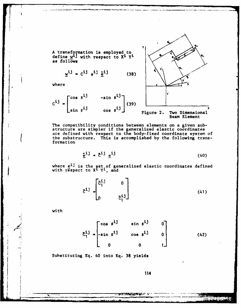
YA transformation is employed todefine wiJ with respect to Xi yi 4as follows

w. .ij =C 1 ij-_e (38)

where

C j Cos Bi -sin (9Y

C ij - (39)sin B Cos B Figure 2. Two Dimensional

Beam Element

The compatibility conditions between elements on a given sub-structure are simpler if the generalized elastic coordinatesare defined with respect to the body-fixed coordinate system ofthe substructure. This is accomplished by the following trans-formation

;_iJ =ijij (40)

where eij is the fet of generalized elastic coordinates definedwith respect to XI yi, and

jij 01iij L (41)

with

cos Bij sin 1ij~ij Bijij

6J -sinoiJ cos B j (42)

0 0 U0

Substituting Eq. 40 into Eq. 38 yields

114

- c'" ij tij eij (43)

It is important to note that the variatig in the angle oij isassumed to be small, thus the matrices C21 and CEJ are assumedconstant. Finally, Eq. 43 can be written as

wi j - Ni j e i j (44)

where

N = Cij * ij ij (45)

*ii iiThe position vector r of an arbitrary point p on the ijth

pelement can be expressed as

i j = Ri + Ai Ni j e i j (46)

where

R= x i yi]T

and

cos 0i -sin 8i

Ai fi(47)

sin ei cos 6i

Differentiating Eq. 46 with respect to time gives

riji + i NiJ eJ + Ai NiJ ij (48).21 -P - _

- ,where

.T7115

t II 1.. .*e : , _ . ;. . .

-sin 8 -o

cos 8e -sin ei

=Ai Ai (49)

and Ai ' is the partial derivative of Ai Vith respect to thereference rotational degree of freedom 01. Substituting Eq. 49

into Eq. 48 and writing r in partitioned form yieldsp

r = [I Ai'NiJe ij AiN ij ] '. (50)-p

Equation 50 is equivalent to Eq. 7 in the general formulationwith the matrix BiJ given by

Bij = Ai'Nje j (51)

The kinetic energy expression for the ijth element is given by

Ti i f .. f ij _ijT -ij dVij

ViJ - P

1 VT MiJ i j (52)

where Vii is the element volume, pij is the density of element

material qj [RiT e ee ijTT and

116

'72-- -;=: ,,. ., ,,'7

"". - _ A

I i j Ai N i j

Mij- f Pij BiJT BiJ T B'J Bij T A' NiJ dV1 JV ij

N.JT A'T NiJ T A'T BiJ NiJ T NiJ

(53)ijThe mass matrix m associated with the flexible coordi-ff

nates is the same matrix that occurs frequently in the finiteelement approach [201.

Utilizing orthonormality of Ai ' , the central term of Eq. 53becomes

f PijBiJ , iJ T piJNijTNijdVijeij

vi j- viij

=eiJiJ e i j (54)-_ lff _

Similarly

f iJ oBiJdViJ Ai J piJNiJdViJeiJ - A1'c isiJj e iJ

viJ vii (55)

-A isS ije

where

6 0 6 0 0., ij

j j s (56)-i "0 6 1 ij 0 6 -_ i

where mij and IiJ are the mass and length of the liJth element+, respectively.

117

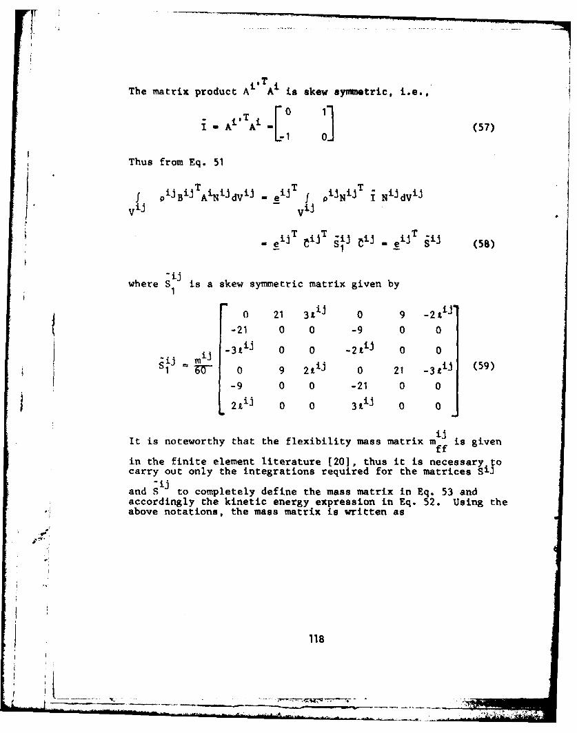
The matrix product AT At is skew symmetric, i.e.,

i- AiT -[. 13 (57)

Thus from Eq. 51

f oiJBijTAiNiJdVJ eij T f iJN i J i NiJdVi j

vii - v j

' i ._i T Cij T ii tij .eii T ii (58)

-ijwhere S is a skew symmetric matrix given by1

0 21 31 i j 0 9 -21 j

-21 0 0 -9 0 0

ij n1 -3 i j 0 0 -2 i j 0 00 9 21i j 0 21 -3 f (59)

-9 0 0 -21 0 0

2 ij 0 0 3t i j 0 0

ijIt is noteworthy that the flexibility mass matrix mif is givenffin the finite element literature [20], thus it is necessary itocarry out only the integrations required for the matrices S 3

- ijand S to completely define the mass matrix in Eq. 53 andaccordingly the kinetic energy expression in Eq. 52. Using theabove notations, the mass matrix is written as

118

Ii

i4 -

ml (symme tric)

iJ e ijT sijT AT ijTim ij (60)

(6x2) (6xl) (6K6

where I is a (2x2) identity matrix. The total kinetic energyof the ith body is given by

niri f ij

T I Tj=1

1 TM . Y~j (61)

where _qi = R i i IT represents the generalized coordinates

iof the ith substructure, qf the elastic coordinates,

mLi (symmetric)

i iT iT iT iT i i= qf S A qf mff~qf (62)

T TTS iA i S' m i_qf f f

andmi is the total mass of the substruq;ureSi is the composite matrix of the SIJ matrices of the

-individual elements

..,m is the composite matrix of the m matrices of theff ff

individual elements

* -i -iiS is the composite matrix of the S matrices of the

individual elements

f _ _

* **, *,:i

It is important to note that each of the above matrices is con-stant and the implied assembly need only be done once. This isbecause the elastic generalized coordinates of each substruc-ture are defined locally which leads to time invariant com-patibility conditions between the elements.

Neglecting shear deformation, the strain energy of the jth

element on the ith body is given by

ij 1lij jIjvi 2i'2[E + iJiJ(vi 2 JAJ(u )]dx J (63)

0

where primes indicate derivaltves with respect to xij, EiJ istbq modulus of elasticity, I J is the second area moment andAI] is the element cross-sectional area.

Using Eq. 35, Eq. 63 becomes

ij=T ij ""

U ff-iJT CijT Fij el

-- ff --Je'

1 ij T

1eiJ ij eiJ (64)

_ ff

where K f is the element stiffness matrix defined with respect

to the body-fixed coordinate system.

Again, the stiffness matrix is constant because the elasticgeneralized coordinates are defined with respect to the body-fixed coordinate system. The total strain energy of the ithbody is obtained as follows

niUi I Ui j

J-1

iT

4~i 1 0 ~

i i J iiISqf 0o Kff] _qf

_ K iTii (65)

120

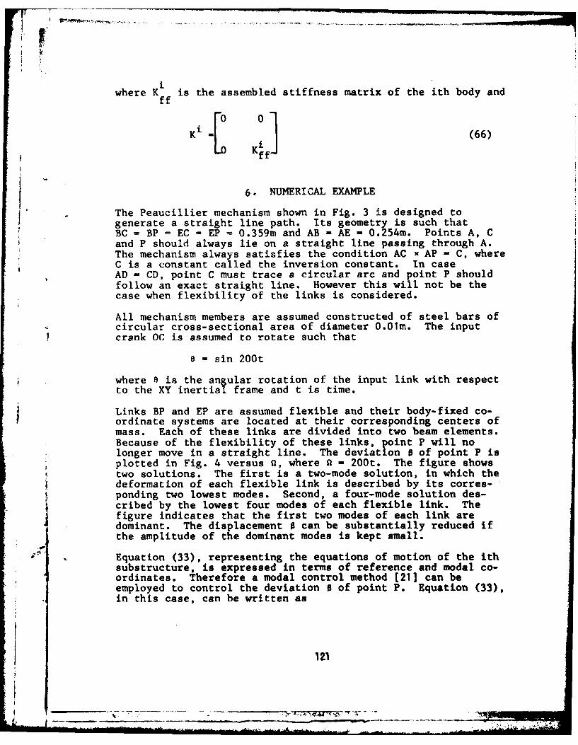
iwhere K is the assembled stiffness matrix of the ith body and

ff

K' 1f (66)

6. NUMERICAL EXAMPLE

The Peaucillier mechanism shown in Fig. 3 is designed togenerate a straight line path. Its geometry is such thatBC = BP = EC - EP = 0.359m and AB = AE - 0.254m. Points A, Cand P should always lie on a straight line passing through A.The mechanism always satisfies the condition AC x AP - C, whereC is a constant called the inversion constant. In caseAD - CD, point C must trace a circular arc and point P shouldfollow an exact straight line. However this will not be thecase when flexibility of the links is considered.

All mechanism members are assumed constructed of steel bars ofcircular cross-sectional area of diameter 0.01m. The inputcrank OC is assumed to rotate such that

e = sin 200t

where a is the angular rotation of the input link with respectto the XY inertial frame and t is time.

Links BP and EP are assumed flexible and their body-fixed co-ordinate systems are located at their corresponding centers ofmass. Each of these links are divided into two beam elements.Because of the flexibility of these links, point P will nolonger move in a straight line. The deviation B of point P isplotted in Fig. 4 versus Q, where A - 200t. The figure showstwo solutions. The first is a two-mode solution, in which thedeformation of each flexible link is described by its corres-ponding two lowest modes. Second, a four-mode solution des-cribed by the lowest four modes of each flexible link. Thefigure indicates that the first two modes of each link aredominant. The displacement 0 can be substantially reduced ifthe amplitude of the dominant modes is kept small.

Equation (33), representing the equations of motion of the ithsubstructure, is expressed in terms of reference and modal co-ordinates. Therefore a modal control method [211 can beemployed to control the deviation B of point P. Equation (33),in this case, can be written as

121

__ _ _ _ - - - -. -t~-- ~

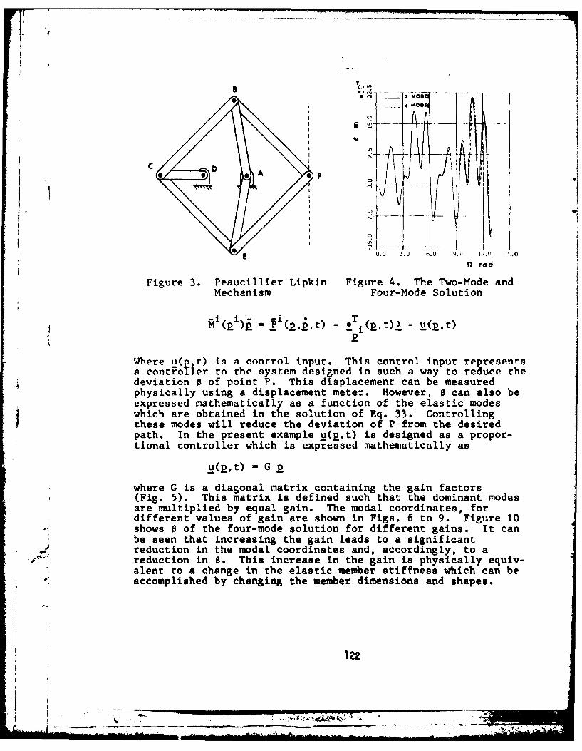
E A

..

4-

E 0.0 3.0 6.0 .I I . I,1

n rad

Figure 3. Peaucillier Lipkin Figure 4. The Two-Mode andMechanism Four-Mode Solution

i (pi)i - Pi( 2 ,2,t) ! T i(Pt)j - u( 2 ,t)

Where u( p ,t) is a control input. This control input representsa controller to the system designed in such a way to reduce thedeviation B of point P. This displacement can be measuredphysically using a displacement meter. However, B can also beexpressed mathematically as a function of the elastic modeswhich are obtained in the solution of Eq. 33. Controllingthese modes will reduce the deviation of P from the desiredpath. In the present example u(p,t) is designed as a propor-tional controller which is expressed mathematically as

- G p

where G is a diagonal matrix containing the gain factors(Fig. 5). This matrix is defined such that the dominant modesare multiplied by equal gain. The modal coordinates, fordifferent values of gain are shown in Figs. 6 to 9. Figure 10shows B of the four-mode solution for different gains. It canbe seen that increasing the gain leads to a significant

* reduction in the modal coordinates and, accordingly, to areduction in 0. This increase in the gain is physically equiv-alent to a change in the elastic member stiffness which can be

* accomplished by changing the member dimensions and shapes.

122

-T

a - 0

0 =1

a a

b.0 0 . .0 1.

n6o

G, 0 G

E ____ 010 E - - -0

00

7-4 -- 4-- 1 I

0. . ' a9.' 20,. 0.0 3.0 6.0 9.0 Pdrj "(

rodaro

Figure 7. Effect of the Gain Figure 8. Effect of the Gainon the Second Mode on the First Mode

*of Link BP of Link EP

123

AL-

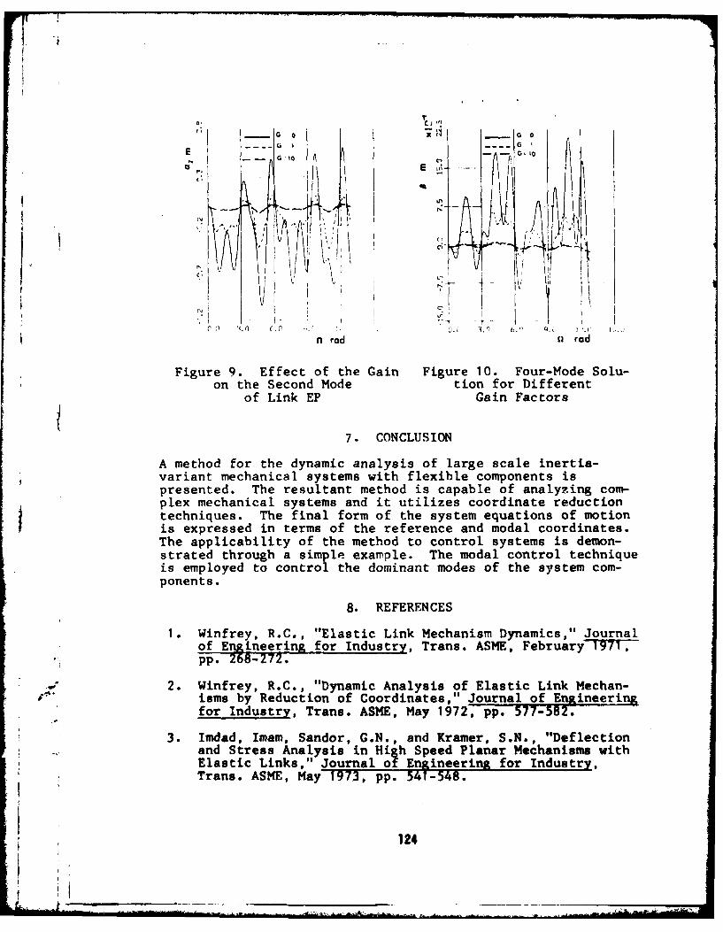
G 0

i I -

Ej E t

- -

nf rod rod

Figure 9. Effect of the Gain Figure 10. Four-Mode Solu-on the Second Mode tion for Different

of Link EP Gain Factors

7. CONCLUSION

A method for the dynamic analysis of large scale inertia-variant mechanical systems with flexible components ispresented. The resultant method is capable of analyzing com-plex mechanical systems and it utilizes coordinate reductiontechniques. The final form of the system equations of motionis expressed in terms of the reference and modal coordinates.The applicability of the method to control systems is demon-strated through a simple example. The modal control techniqueis employed to control the dominant modes of the system com-ponents.

8. REFERENCES

1. Winfrey, R.C., "Elastic Link Mechanism Dynamics," Journalof Enineerin& for Industry, Trans. ASME, February-T7Tp.268-27Z.

2. Winfrey, R.C., "Dynamic Analysis of Elastic Link Mechan-isms by Reduction of Coordinates," Journal of Engineeringfor Industry, Trans. ASME, May 1972, pp. 577-582.

3. Imdad, Imam, Sandor, G.N., and Kramer, S.N., "Deflectionand Stress Analysis in High Speed Planar Mechanisms withElastic Links," Journal of Engineering for Industry,Trans. ASME, May 1973, pp. 541-548.

124

4. Erdman, A.G., Sandor, G.N., and Oakberg, R.G., "A GeneralMethod for Kineto-Elastodynamic Analysis and Synthesis,"Journal of Engineering for Industry, Trans. ASME, November1972, pp. 1193-1205.

5. Sadler, J.P., and Sandor, G.N., "A Lumped ParameterApproach to Vibration and Stress Analysis of ElasticLinkages," Journal of Engineering for Industry, Trans.ASME, May 1973, pp. 549-557.

6. Winfrey, R.C., Anderson, R.V., and Gnilka, C.W., "Analysisof Elastic Machinery with Clearance," Journal ofEngineering for Industry, Trans. ASME, August 1973,pp. 695-703.

7. Chu, S.C., and Pan, K.C., "Dynamic Response of a High-Speed Slider-Crank Mechanism with an Elastic ConnectingRod," Journal of Engineering for Industry, May 1975,pp. 542-550.

8. Imdad, Imam, and Sandor, G.N., "High-Speed MechanismDesign - A General Analytical Approach," Journal ofEngineering for Industry, May 1975, pp. 69-67.

9. Kohli, D., Hunter, D., and Sandor, G.N., "ElastodynamicAnalysis of a Completely Elastic System," Journal ofEngineering for Industry, Trans. ASME, August, 1,77pp. 604-609.

10. Midha, A., Erdman, A.G., and Frohrib, D.A., "An Approxi-mate Method for the Dynamic Analysis of Elastic Linkage,"Journal of Engineering for Industry, Trans. ASME, May1977, pp. 449-455.

11. Midha, A. Erdman, A.G., and Forhrib, D.A., "Finite ElementApproach to Mathematical Modeling of High Speed ElasticLinkage," Mechanism and Machine Theory, 1978, Vol. 13, pp.603-618.

12. Cavin, R.K., and Dusto, A.R., "Hamilton's Principle:Finite Element Methods and Flexible Body Dynamics," AIAAJournal, Vol. 15, No. 12, December 1977, pp. 1684-160.

13. Song, J.O., and Haug, E.J., "Dynamic Analysis of PlanarFlexible Mechanisms," Computer Methods in AppliedMechanics and Engineering, Vol. 24, 1980, pp. 359-381.

14. Shabana, A.A., and Wehage, R.A., "Variable Degree of Free-* dom Component Mode Analysis of Inertia Variant Flexible

Mechanical System," submitted to ASME Journal of Mechani-cal Design, Feb. 1982.

125

f .t*

15. Shabana, A.A., "Dynamic Analysis of Large Scale InertiaVariant Flexible Systems," Doctoral dissertation, Dept. ofMech. Eng., University of Iowa, Dec. 1982.

16. Wehage, R.A., and Haug, E.J., "Generalized CoordinatePartitioning for Dimension Reduction in Analysis ofConstrained Dynamic Systems," Journal of MechanicalDesign, Vol. 104, 1982, pp. 247-255.

17. Zienkiewicz, O.C., The Finite Element Method, ThirdEdition, McGraw-Hill Book Co., 1977.

18. Goldstein, H., Classical Mechanics, Addison Wesley, 1950.

19. Bathe, K.J., and Wilson, E.L., Numerical Methods in FiniteElement Analysi s , Prentice-Hall, Englewood Clitts, N.J.,

1976.

20. Przemieniecki, J.S., Theory of Matrix Structural Analysis,McGraw-Hill, 1968.

21. Takahashi, Y., Rabin, M.J., and Auslander, D.M., Controland Dynamic Systems, Addison Wesley Publishing, I .

I

1

.

-12I"4.,

12