z o N.S.F. IfSF/RA 790212

" \

npr\~)-1130H

I- 5 · o emlnar-

z ::)

o~---­~ LJ LJ Z

~ l­

-750

V) L...-.._

REPRODUCED BY NATIONAL ·TECHNICAL INFORMATION SERVJCE

u. S. DEPARTMENT OF COMMERCE SPRINGFIELD, VA. 22161 __

, 30

ASRA INFORMATION RESOURCES NATIONAL SCIENCE FOUNDATION

t UP

, 3S

TABLE OF CONTENTS

Preface.................................................................................................................... i

Introduction.. .. .. .. .. .. .. .. .. .. .. .. .. .. . .. .. .. .. .. .. .. .. .. .. .. .. .. .. .. .. .. .. .. .. .. .. .. .. .. .. .. .. .. .. .. .. .. .. .. .. .. .. .. .. .. .. • .. .. .. .. .. .. .. .. .. .. . .. .... ii

List of Participants................................................................ 1

Prograxn ..................................................................................................................................................... ..

Quantitative prediction of strong Motion for Potential Earthquake Fault, ••.....•.•. 3

Recent Developments and Applications of Deterministic Earthquake Models: Prediction of Near-And Far-Field Ground Motion. . . . . . . . . . . . . . . . . . . .. . . . . . . . . . . . . . .. . . . . .. . . . . . 6

Application of System Identification Techniques for Local Site Characterization ..... 14

Radiated Seismic Energy and the Implications of Energy Flux Measurements for Strong Motion Seismology ............................................................................................................................... 19

Intensity and Regression ..•••.•••...••••.••.•..••.•.•••....••...•...•.•.•..•.•••.... 25

Modeling of Near-Fault Motions ....................................................... 30

A Dynamic Source Model for the San Fernando Earthquake .............................. 36

Alternative Ground Motion Intensity Measures .•....•..•.•.•..•.•..•...•.•.•..•••.••.. 39

Let's Be Mean ....................................................................... 41

Measures of High-Frequency strong Ground Motion •••••••••.••••••••••••••••••••••••••• 46

Synthesis of San Fernando Strong-Motion Records.......................................... 52

SH Propagation in a Layered Half-Space. . • • • .. . . . . . . • • . • • • . . .. . • . .. • . .. . . .. .. . . • . • . • . . • .. • .. 56

Statistics of Pulses on Strong Motion Accelerograms ..................................... 60

An Introduction to Strong-Motion Instruments and Data .................................... 65

The Application of Synthetic Seismograms to the Study of Strong Ground Motion .....•. 77

Semi-Empirical Approach to Prediction of Ground Motion Produced by Large Earthquakes. . . . . . . . . . . . . . . . . . . . . . . . . . . . . . . . . . . . . . . . . . . . . . . . . . . . . . . . . . . . . . . . . . . . . .. 80

Deterministic Modeling of Source Mechanisms Utilizing Near- and Far-field Seismic Data: The 1971 San Fernando Earthquake ........................................... 85

Occurrence of Strong Ground Motions .......................................................... 89

The Needs of the Nuclear Regulatory Commission in the Field of Strong Motion Seismology. . . . . . . . . . . . . . . . . . . . . . . . . . . . . . . . . . . . . . . . . . . . . . . . . . . . . . . . . . . . . . . . . . . . . . .. 92

Some Thoughts on the Definition of the Input Earthquake for the Seismic Analysis of Structures......................................................................................................... 95

Simulations of Earthquake Ground Motions..... . .. . • .. .. • .. . . . .. .. • • .. . . • .. .. . .. • .. • . • .. .. .. .. . . .. . .. .. • ... 98

Directions of Future Research ...................................................................................... 102

Any opinions, findings, conclusions or recommendations expressed in this publication are those of the author(s) and do not necessarily reflect the views of the National Science Foundation.

I~

PREFACE

The volume represents the Proceedings of a small Seminar - Workshop held at the Inn

at Rancho Santa Fe, near San Diego, in February 1978. The meeting was conceived in response

to a growing awareness of the mutual interest in research workers in seismology and earth-

quake engineers in the records of strong ground motion. The Seminar - Wrokshop was partly

sponsored by the geophysical and earthquake engineering research programs within the National

Science Foundation, and was jointly organized by Donald V. Helmberger of the Seismological

Laboratory and Paul C. Jennings of the Earthquake Engineering Research Laboratory, of the

California Institute of Technology. The Organizers wish to take this opportunity to acknowl­

edge the helpful assistance of Thomas Hanks, Leonard Johnson and S. C. Liu.

. ) '8

INTRODUCTION

The strong ground motion near the source of a major earthquake determines the forces

which endanger buildings and other works of construction, and at the same time is the most

detailed clue available concerning the source mechanism of the earthquake. The records

obtained of strong ground motion are, therefore, of interest to both seismologists and earth­

quake engineers, although the two disciplines have tended to look at the records quite dif­

ferently, and to pursue their examinations separately. In the past few years, however, there

has been a growing awareness of the mutual interest in strong ground motion and a number of

individuals believed there would be considerable value in convening a small group of seismolo­

gists and earthquake engineers who are doing research on strong ground motion for a Seminar -

Workshop. It was envisioned that a Seminar - Workshop would be a useful means for scientists

and engineers to discuss their mutual interests and problems, and to hear and discuss those

areas where their interests and viewpoints are different.

There are many fundamental questions in seismology and earhtquake engineering which focus

attention on the nature of strong ground motion. From the seismological viewpoint, the re­

cords of strong ground motion provide the best source of high frequency information on the way

that energy is released during the rupture process. Additionally, strong motion data has the

capability of providing a major means for determining the nature of the source mechanisms in

great earthquakes. The extent of the source mechanism, the stress drop and other parameters

of the source, and the range of complexity of source mechanisms are all capable of being stud­

ied through strong-motion records. From the engineering viewpoint the central problems are

the characterization of strong ground motion for the purpose of establishing design criteria

and the determination of the nature of the shaking in the near-field of major and great earth­

quakes. These problems are faced in the design of almost every major facility in the more

seismic areas of the country and there is not yet a consensus on how to deal with them. To

resolve these important practical problems requires a much increased understanding of strong

ground motion. A problem of mutual interest to both seismologists and earthquake engineers

is the way the earthquake motion is altered as it propagates away from the source. Seismolo­

gists have examined this problem by studies of radiation patterns under idealized conditions

and by calculating the effects of regional geology on ground motions of periods of one second

and more. Under similar assumptions, earthquake engineers have calculated the effects of

surficial soil deposits on strong ground motions of shorter period.

At a £ewinstitutionssigni£icant interaction between seismologists and earthquake engi­

neers has developed, but there is clearly a benefit to be gained by much more communication

between the two disciplines; it was the intent of the Seminar - Workshop to accelerate this

communication. It was also hoped that a number of areas of mutual interest and research need

could be identified.

This report, which contains extended abstracts of the invited papers, represents the

Proceedings and the Seminar - Workshop. The papers and the discussions at the conference

were grouped around three major areas.

ii

(1) Characterization and parameterization of strong ground motions.

(2) Simulation and modeling of strong motions: deterministic and statistical.

(3) Source mechanisms and estimation of strong motion for great earthquakes.

The invited papers are followed by a brief discussion of the directions of future

research.

iii

D. V. HeImberger

P. C. Jennings

PARTICIPANTS

Professor C. Archambeau

Mr. J. Beck

Mr. J. Boatwright

Professor B. Bolt

Professor D. Boore

Dr. M. Bouchon

Professor J. Brune

Professor A. Chopra

Professor A. Cornell

Dr. N. Donovan

Dr. J. Evernden

Dr. G. Frazier

Dr. T. Hanks

Professor G. Hart

Dr. T. Heaton

Professor D. HeImberger

Professor R. Herrmann

Professor G. Hausner

Professor P. Jennings

Professor L. Johnson

Dr. L. Johnson

Professor C. Langston

Dr. S. C. Liu

Professor E. Luco

Professor H. Kanamori

Dr. R. Matthiesen

Dr. L. Reiter

Professor J. Roesset

Professor H. Seed

Professor S. Smith

Dr. D. Tocher

Dr. R. Wiggins

1

AFFILIATION

C.LR.E.S.

Cal tech

Columbia University

U. S., Berkeley

Stanford University

M.LT.

V.C. I San Diego

U. S., Berkeley

M.LT.

Dames and Moore

U.S.G.S.

Del Mar Technical Assoc.

U.S.G.S.

D.C., Los Angeles

Caltech

Cal tech

Saint Louis University

Cal tech

Caltech

u. C., Berkeley

N.S.F., Geophysics

Pennsylvania State University

N.S.F., RANN

U.S., San Diego

Cal tech

U.S.G.S.

N.R.C.

M.LT.

U.C. I Berkeley

u. of Washington

Woodward-Clyde Consultants

Del Mar Technical Assoc.

SEMINAR-WORKSHOP ON STRONG GROUND MOTIONS

Program

Sunday, February 12

6:00 p.m.

Monday, February 13

9:00-11:00 a.m.

11:30 a.m.-l:30 p.m.

1:30-5:30 p.m.

7:00 p.m.

8:00-10:00 p.m.

Tuesday, February 14

9:00 a.m.-ll:30 a.m.

11:30 a.m.-l:30 p.m.

1:30-5:30 p.m.

7:00 p.m.

8:00 p.m.

Wednesday, February 15

9:00-11:30 a.m.

11:30 a.m.-l:30 p.m.

1:30-3:00 p.m.

Attitude Adjustment Hospitality Suite

Introductory Session

P. Jennings and D. HeImberger

NSF Sponsors - L. Johnson and C. Liu

Lunch Break

Session - Characterization of Strong Ground Motion

G. Hausner, H. Kanamori, J. Brune, C. Archambeau,

T. Hanks, B. Bolt, and R. Matthiesen.

Dinner

Session - Modeling of Strong Ground Motion

San Fernando Earthquake

M. Bouchon, C. Langston, and T. Heaton.

Session - Modeling of strong Ground Motion

J. Roesset, H. Seed, J. Luca, D. Boare,

J. Boatwright, G. Hart, and A. Chopra.

Lunch Break

Session - Modeling of Strong Ground Motion (Cont'd)

L. Johnson, R. Herrmen, R. Wiggins, J. Beck,

A. Cornell, N. Donovan, and L. Reiter.

Dinner

Informal Session - Nature of Great Earthquakes

Session - Direction of Future Research

Lunch Break

Final Session

2

QUANTITATIVE PREDICTION OF STRONG MOTION FOR

A POTENTIAL EARTHQUAKE FAULT

Keiiti Aki, Michel Bouchan

Bernard Chouet, and Shamita Das

Massachusetts Institute of Technology

We describe a new method for calculating strong motion records for a given seismic re­

gion on the basis of the laws of physics, using information on the tectonics and physical

properties of the earthquake fault.

Our method is based on a new earthquake model, called IIbarrier model," which is charac­

terized by five source parameters: fault length, width, maximum slip, rupture velocity, and

barrier interval. The first three parameters may be constrained from plate tectonics, and

the fourth parameter is roughly a constant. The most important parameter controlling the

earthquake strong motion is the last parameter, "barrier interval".

The theoretical basis for the "barrier model" comes from a study by Das and Aki (1978)

of rupture propagation when barriers of high strength material are present on the fault

plane. They showed that the following three different interactions between the crack-tip

and the barrier can occur, depending on the strength of the barrier relative to tectonic

stress.

(1) If the tectonic stress is relatively high, the barriers are broken as

the crack-tip passes.

(2) If the tectonic stress is relatively low, the crack-tip proceeds beyond

the barrier, leaving behind an unbroken barrier.

(3) If the tectonic stress is intermediate, the barrier is not broken at the

initial passage of the crack-tip, but eventually breaks due to subsequent

increase in dynamic stress.

A comparison of the slip function, obtained for the case where all the barriers are

broken as the crack-tip passes with the case in which one barrier is left unbroken, is shown

in Figures I and 2. The ubarrier model" provides an explanation for the variation of the

seismic spectra of small earthquakes with magnitude observed by Chouet, et al. (1978). It

also explains the major features of the near-field and teleseismic records of the San Fer­

nando earthquake (Bouchon, 1978) and the characteristics of surface faulting in many regions

(e.g., Wallace, 1973; Tchalenko and Berberian, 1975).

There are three methods to estimate the "barrier interval" for a given seismic region:

(1) surface measurement of slip across fault breaks; (2) model fitting with observed near­

and far-field seismograms; and (3) scaling law data for small earthquakes in the region. The

IIbarrier intervals" were estimated for a dozen earthquakes and four seismic regions by the

above three methods, as shown in Figure 3. Our preliminary results for California suggest

that the "barrier interval II may be determined if the maximum slip is given. The relation

p·SY-O

I I

P·SY-I

~--------J. ,,·,:\1 ~ n,----------, ".~! I I-z lJJ ~ lJJ U ct I. ...J Q.

~ ,

CI

CI lJJ N

~.5 , , ~

I

a:: I -T-'-, 0 1/" Z

o

,

2

,

4 _,,--:f-

.5

X,/L

, , , , ,

Fig. 1: The Value of (1 + S), a measure of

I­Z lJJ :::E w u ct ...J Q. fJ)

CI

CI .5 lJJ !:::! ...J ct :::E a:: o z

4

o X,/L

Fig. 2: Case P-SV-l, in which one barrier

material strength relative to tectonic stress exists on the fault palne (see Fig. 1 legend

is shown as a function of distance xl along for details). The crack-tip skips the barrier

the path of rupture propagation on top of the without breaking it.

figure. This is the case p-sv-O, in which

no barriers exist on the fault plane. At the

bottom, snap shots of the parallel component

displacement of the crack surface ul

(x1,o,t)

are shown as a function of xl" ul

is normal­

ized by the factor L(TO-Tf)/~ and the number

attached to each curve indicates time, t,

measured in the unit of O.5L/a, where L is

the length of the fault, a is the compres­

sional wave velocity, ~ is the rigidity, T o

is the initial tectonic stress, and Tf

is the

dynamic function of the fault plane.

4

::< 0<:

10 z

--' <! > 0:: W f-;;: 0:: W

Nobr,1891

• Kito-lzu,1930

DaS/~9~t~. _, ....... C:rriZO Plain

Wokoso - boy 1963 /So;tomo, 1931 \ T /' . / 1857 • ~. /' ottora, 1943

IZU-I~~~tO-OkY ,. .;t-Son ~rnondo(jnitiol part) -. Saitoma, 1968 -Tongo,r927 1971

/

cr Cent': -Vc~~o;o~ ~;sh;YOmo

r-~'--------''--.-------L'--~ Parkfield 0:: <! CD

0.2

• Seismic measurement of rise time

/ Scaling law of seismic spectrum

California earthquakes

10 MAXIMUM

1966

Fig. 3: Relation between the barrier interval and the maximum slip obtained by various methods

between the "barrier interval" and maximum slip varies from one seismic region to another.

For example, the interval appears to be unusually long for Kilauea, Hawaii, which may explain

why only scattered evidence of strong ground shaking was observed in the epicentral area of

the Island of Hawaii earthquake of November 29, 1975.

The stress drop associated with an individual fault segment, estimated from the barrier

interval and maximum slip, lies between 100 and 1000 bars (Figure 2). These values are about

one order of magnitude greater than those estimated earlier by the use of crack models with­

out barriers. Thus the barrier model can resolve, at least partially, the well-known discre­

pancy between the stress-drops measured in the laboratory and those estimated for earthquakes.

REFERENCES

Bouchon, M., A dynamic source model for the San Fernando earthquake, Bull. Seis. Soc. Am.,

submitted 1978.

Chouet, B., K. Aki, and M. Tsujiura, Regional variation of the scaling law of earthquake

source spectra, Bull. Seis. Soc. Am., in press, 1978.

Das, S. and K. Aki, Fault plane with barriers: a versatile earthquake model, J. Geophys. Res.

submitted 1978.

Tchalenko, J. S. and M. Berberian, Dasht-e Bayaz Fault, Iran: earthquake and earlier related

structures in bedrock, Geol. Soc. Am. Bull., 86, 703-709, 1975.

Wallace, R. E., Source fracture patterns along the San Andreas fault, Proc. Cont. Tectonic

Processes of the San Andreas Fault System, ed. by R. L. Kovach and A. Nur, Stanford

univ. Press, Geological Sci., vol. XIII, 248-250, 1973.

RECENT DEVELOPMENTS AND APPLICATIONS OF DETERMINISTIC

EARTHQUAKE MODELS: PREDICTION OF NEAR-AND

FAR-FIELD GROUND MOTION

Charles B. Archambeau

University of Colorado

There are two objectives of the work to be described. First, to provide an under­

standing of the near-field ground motion observed from earthquakes in terms of the basic

physics of the source; and second, to be able to determine critical physical variables,

such as the stress field, prior to an earthquake. From these variables it would be possible

to predict not only the probable location and size of future earthquakes, but the expected

ground motion as well, and given this ability, to actually be able to make reliable ground

motion predictions.

In attempting to realize these objectives it is clearly necessary to accurately account

for wave propagation effects in rather great detail. Thus, it is necessary to have a reason­

ably good, detailed, knowledge of the earth structure, including both anelastic and elastic

properties. Based on studies of seismic radiation from nuclear explosions, it is felt that

we have sufficiently good analytical and numerical wave propagation methods for these pur­

poses and that our knowledge of earth properties, in at least some regions, is adequate to

be able to realistica.lly account for the most important propagational effects.

Of at least equal importance for the achievement of the stated objectives (particularly

prediction) is the use of a dynamical theory for the source so that it will be possible to

relate the seismic radiation from an earthquake directly to the physical properties of the

material and the initial stress state of the medium. Both of these can, in principle be

inferred independently before the occurrence of the event. In the work to be described here

we have used the dynamical relaxation theory formulation (e.g., Archambeau, 1968; Archambeau

and Minster, 1978), and as preliminary models, the growing spherical inclusion models derived

from this theory (Archambeau, 1968; Minster, 1973). In addition, we have used dynamical

boundary conditions on the failure surface enclosing the (narrow) region in which the material

transition (failure) occurs and, in particular, the result (Archambeau and Minster, 1978)that

the rupture velocity is proportional to the stress drop.

In order to determine the detailed physical origins of the radiated field, we have con­

sidered the seismic field data from the San Fernando earthquake in rather great detail (Bache,

Barker, and Archambeau, 1978).

Figure 1 shows a schematic of the symmetry plane for the failure zone, or "fault plane",

for the event along with the sense of rupture propagation from the point of nucleation at a

depth of 11.4 km. Two relaxation theory models were used to represent these rather complex

variable stress drop events; one at the hypocenter that grew bilaterally for approximately

3 km and then extended unilaterally upward until it reached the bend in the failure plane

6

Skin

1

Pacoima Dam

1--- 7. 8--""'"+--__ 10.6"'" --l

~ "t Vf!l1t" - --.......... 2 Direction of

9 k", "-- Rupture

;::.~ ---; {

21' --.. ~ I' ., 11. 4 :kIn

~~'" X"x 1 <';, +~

.~, .. ~ ~'" X ~~ '0

~

"\ San Fernando Earthquake:

Geometry of the failure zone and location. extent and sense ~:r~~~~!~/or the two "events" used to model the complete

Pacoima Dam

'Of ~j

'1/ 'V : ,\F 18 16 14 12 10 -2 -4

Rupture Front Location

Fig. 1: Rupture velocity and stress drop plotted as functions of distance along the fault

from the hypocenter. Event 2 was started from a finite volume for the failure zone while

event 1 started from a point.

showni and a second "event" which fonns a continuation of the first beyond the bend beginning

with finite failure zone volume and high stress drop and rupture velocity, extending unilater­

ally toward the surface. The lower graph in the figure shows the variations of stress drop

and rupture velocity used, where the rupture velocity was varied directly with the stress

drop. This final composite model is the result of many iterations in fitting first the short

period far-field, then the long period moment, and finally the near-field strong motion as

observed at the Pacoima Dam receiver~ This model, therefore, simultaneously fits the long and

short period far-field and gives a good first order fit to the Pacoima velocity and displace­

ment records.

Figure 2 shows the fit to the short period (near 1 Hz) seismograms recorded at a number

of stations beyond 30° in distance (except for ATL which was near 25°) and at various azi­

muths. As can be seen, the fit is quite good, certainly for the first 10 seconds, with devi­

ations being most marked at later times at some of the stations. It is likely that some of

7

GAIN RATIO ~AINRATIO

ALfJ1 Pw,A ~Jt\.~ A...A-.Aflf'Lr. n !'I A ATL. .

KT~V~]~:1~V,:~~ ~~~~V cu~l.AAM1~A;I:~~AA/ V~'V~'V--O~Vv--v ~~·~V~VV· VV~;V-

GD~U~ffiA ~ ~M AR~k;.fl...rJ.J,~_f./V\ M\

~v v·VV¥'~V vV

O.74

V • ·PE~VY-VV\r'V;VVVV"L~9VV vv ESK

1.27 0.71

OG~tLJ\IhMl'V\Al\/\fI~rv MA!.J1 fl .• A""fV),.f,~I\-A",",Iv-.J"\ / V- "! \1W v· V V ·0.91 '" v· - V 'J'Yj r V v Y" \J v - ~.02 .. v

o 5 10 15 2025300 5 10 15 20 25 30

Fig. 2: San Fernando Earthquake: Theoretical (double event) and observed displacement at

teleseismic distances.

later 11 signal II is due to the near surface faulting, which was not included in the model, and

that most of it is "signal generated noise"~ that is, due to surface waves generated by body

wave signal arrivals in the receiver vicinity_ This phenomena was not included in the wave

propagation calculations and so would not be predicted. It was found that these short period

signals could be modeled using only the high stress drop parts of the composite event. On

the other hand, the low frequency surface waves and body waves were almost entirely controlled

by the low stress drop, low rupture velocity, dimensionally more extensive part of the failure

process.

Figure 3 shows the fit of the model predictions to the near-field strong motion data at

the Pacoima dam receiver. Clearly the fit to the first 5 to 6 sec. of the displacement record

is very good. The deviation at later times, starting near 7 sec. after the start of the sig­

nal train, is probably due to the omission from the model of the very-near surface faulting,

which involved branching into multiple faults, as well as from omission from the wave propaga­

tion calculation of the surface waves generated at the free-surface by the direct waves from

the event.

Virtually the same comments apply to the velocity data, in that the fit is fairly good

to around 5 sec. for the wave field with frequency below about 2 Hz. However, comparison of

the theoretical and observed velocity clearly shows that the model, which fits the short per­

iod far-field data very well, does not fit the higher frequency near-field data very well at

8

1000 iJ GROUND ACCELERATION

o ~~f*rlw~t\~~~r~--1000-l_ GRQUNO VELQCITY

~~~~ 50

~ ~L------ GROUND OIS?LAC~MENT

---~--gl o .----

50

o 5 SECCNOS

10 15

Fig. 3: Comparisons of the observed and predicted (dashed lines) velocity and displacement

at the Pacoima Dam site. Final fault model for the San Fernando earthquake.

all. Thus a IIfar-field model" which fits the seismic data below about 2 to 3 Hz does not

provide a very good fit to the high frequency near-field data above 3 Hz. Thus, in both the

velocity and acceleration records, the large 3-4 Hz pulse arriving at sec. and 6 sec. from

the beginning of the record are not predicted by the !lfar-field model", nor is the yet higher

frequency background signal that is evident on the acceleration records.

Because of the constraints on the model from the (band limited) far-field data and in

view of the fit to the near-field low frequency data, the only way to fit the high frequency

strong motion data is to include short intervals, of the order of .5 km., of very high stress

drops along the failure zone. The stress drops would have to be of the order of several kilo­

bars. In particular, from the data itself, it is evident that one very high stress drop

lIeventll of small dimension (about .1 kIn.) must have occurred at the hypocenter corresponding

to the initiation of failure. Similarly, a second high stress "event" of somewhat larger

dimension must have occurred at the fault bend in order to account for the high frequency

acceleration and velocity signal arriving at about 3 sec. on the seismograms. The later

arriving signals, starting at around 6 sec. and including the maximum acceleration, would

9

then be explained by a combination of (low stress drop) multiple faulting at the surface and

surface wave generation from the earlier large, high frequency signals.

These modifications of the model would alter the stress drop and rupture velocity shown

in Figure 1, so that short sections near the points (1.) and (2.) would have very high stress

drops, ·of the order of several kilobars, and correspondingly high rupture rates.

In the context of the dynamical source theory used, these results imply that earthquake

failure processes are initiated at stress levels of the order of several kilobars and that

growth of the failure zone is accomplished dynamically; that is the failure zone is dynamic­

ally driven through zones of relatively low initial stress, with this process occurring be­

cause of the high dynamic stress concentrations near the "front" (region of maximum surface

curvature) of the failure zone. Further, for stresses of this magnitude, which are of the

same order as those observed for failure under laboratory conditions, the dynamic theory re­

quires failure transition energies of the order of 107

ergs/gm (see Archambeau and Minster,

1978). This transition energy is in fact the change in the internal energy of the material

upon failure. The transition energy for melting, for example, ranges from 107

to 109

ergs/gm

in ordinary solids and probably somewhat lower for "weakened" solids. The size of the trans­

ition energy implies a nearly complete, although perhaps transient, loss of shear strength

and probable melting in the failure zone, or at least melting of some of the rock consti­

tuents. Thus, the highly variable stress drop observed for the San Fernando earthquake is

interpreted to be a consequence of the inhomogeneity of the initial, ambient, stress field

arising, at least in part, from the variability in long term strength of the material to

low strain rate loading, as well as from the elastic inhomogeneity of the medium. From this

interpretation it would follow that the failure process would initiate at a point at which

the highly inhomogeneous stress field reached a critical level of several kilobars. At the

time of failure the shear stress drop would be nearly total. The energy changes associated

with the ensuing stress relaxation must then be such that the (dynamic) energy density at the

edges of the transition zone be large enough to overcome the transition energy barrier--of

about 107

ergs/gm--in order for the process to continue. Since the energy density near the

edges of an inclusion can be much larger than the initial energy density, it is clear that

the failure zone may continue to expand into new material even when the origin stress level

was not sufficient to initiate failure there.

The conclusion is therefore, that the near-field strong motion data requires very high,

localized, stress drops along the failure zone and that it is these spatially limited, high

stress drops that result in the very high accelerations in the near-field. It is also con­

cluded that these same high stress points are the locations of failure initiation.

The second objective of predicting near-field accelerations in a deterministic fashion

becomes, under the premise that all of the previous conclusions are generally accurate, pri­

marily a question of being able to infer the initial stress field prior to an earthquake.

More accurately, prediction of the location, size, and expected radiation field of an earth­

quake in both the near- and far-fields requires the determination of the "recoverable"

10

'\

initial stress existing prior to the event. One approach that is currently being applied in­

volves using small earthquakes as events that IIsample ll the existing stress field. In parti­

cular, observations of the radiation fields from small events (foreshocks) may be used to

infer the associated stress drops. Since the events are small, it is safe to assume that the

accompanying stress changes are small perturbations in the existing background stress, so

that these stress drop determinations provide a sampling of the recoverable initial stress.

50 -J-------------------ff--l J __ ~~~ ________ _ : 234 ' ,pO

, , , , ~ : '<:

, , , ,

J -----------------J

1 SeismiC Region 19 I

Jopcm - KUriles - Komchatka ! Hypoc~r.'eu:.l Shear She'5s --1

Depth Range: O!:: Z< 20 j 3013~5~l-LJ-L-L~l-~~-L~L-~-L-L~1*5~5"-~I-LI-LI ~1-L1-L1~1~1~165

Fig. 4: Shear 9tress contou~s for Region 19 ~n the depth range 0-20 km. stress changes

estimated using .~ and Ms data. Numbers refer to event sequence numbers, the larger values

indicating the most recent events. Contours at 10, 100, 1000 bars.

11

'So -.-- - - - - -- - - - - -- - - - - - -4i~" - - _!OJ)_ - - - - - - - - - --, 262

264 " 165 QIQ 168

40

~~elsmIC RegIon 19

J1r In· Kurlles- Komcrotko

: Hypocenterol Shear Stress i : Depth Range: 40~ Z< 50 J

3O,."3-.,!5L.l.-L--'----'--'---"--'--L.,"4'"'s""--I.I-L1 --"-, -L-LLLTs5J .LL.L.LL-LL- l65

Fig. 5: Shear stress contours for Region 19 in the depth range 40-50 km. Stress changes

estimated using ~ and Ms data. Numbers refer to event sequence numbers, the larger values

indicating the most recent events. contours at 10, 100, 1000 bars.

Figures 4 and 5 illustrate recoverable stress maps for different depth ranges obtained

using this approach, with event magnitudes as the data from which stresses are estimated for

the individual events. When enough small events are available the stress estimate data can.

be contoured to provide a reasonable first order estimate. Clearly the high stress zones at

or above 1 ki1obar, are the sites for future large earthquakes. The larger the dimension

of such a very high stress zone, the larger the expected earthquake.

The stresses estimated in this way are average stresses over a volume and fluctuations

over small dimensions are not resolved. In view of the necessity of determining the rather

small spatial zones of very high stress in order to obtain good near field ground motion pre­

dictions, it is clear that a high resolution method must be used to obtain the required

stress maps. This means that many very small events must be studied and that high frequency

seismic radiation field data must be used so that the stress drop averages obtained are over

small volumes. A high frequency method of this type is presently being applied to California

micro-earthquake data. preliminary results from earlier work, using larger earthquakes in

Eurasia, suggest that the required resolution can be attained.

REFERENCES

Archambeau, C. B., General theory of Elastodynamic Source Fields, Rev. Geophys, 16, 241-288

1968.

Archambeau, C. B., The theory of Stress Wave Radiation from Explosions in Prestressed Media,

Geophys., J.R. astr. Soc., 29, 329-366, 1972, (Appendix, Geophys, J. R. astr. Soc., 31

361-363, 1973)

Archambeau, C. B., and J. B. Minster, Dynamics in Prestressed Media with Moving Phase Boundar­

ies: A Continuum Theory of Failure in Solids, Geophys. J. R. astr. Soc., ~, 65-96,

1978.

Bache, T. C., T. G. Barker and C. B. Archambeau, The San Fernando Earthquake - A Model Con­

sistent with Near-Field and Far-Field Observations at Long and Short Periods. in prepar­

ation. From: Final Report, USGS Earthquake Hazards Program, for the period Oct. I,

1976 to Sept. 30, 1977. Systems, Science and Software, LaJolla, California.

Minster, J. B., E1astodynamics of Failure in a Continuum. Ph.D. Thesis, California Institute

of Technology, Pasadena, Calif. 1973.

Minster, J. B. and A. M. Suteau, Far-Field Waveforms from an Arbitarily Expanding, Trans­

parent Spherical Cavity in a Prestressed Medium, Geophys. J. R. Soc., 50, 215-233, 1976.

13

INTRODUCTION

APPLICATION OF SYSTEM IDENTIFICATION

TECHNIQUES FOR LOCAL SITE CHARACTERIZATION

James L. Beck

California Institute of Technology

A question of concern in the earthquake-resistant design process is to what extent and

in what manner should the design response spectrum or ground motion time history be modified

to account for the influence of local soil and geological properties at the site. To inves­

tigate this problem, a model is required which characterizes the dynamics of the local medium

in terms of its geometry and material properties. For example, an alluvial-filled valley

might be modeled by an elastic region imbedded in an elastic half-space. Alternatively, to

greatly reduce the order of a linear rnbdel, the local medium might be represented by its

dominant modes.

In general, the parameters of such models for a particular site must be determined em­

pirically. If seismic records are available from the site, there is a potential for applying

system identification techniques to estimate the parameters and to make some evaluation of

the model form.

The general approach formulated in the next section would require at least one ground

motion record, the "output", at the surface of the site, together with corresponding records

which describe the "input" motion to the model. The number and location of the records neces­

sary to define the input depends on the complexity of the model. For example, for a simple

one-dimensional model with vertical wave-propagation, a record from the bottom of a bore hole

may be sufficient. In general, some difficulties may arise because a simplified model and

its associated input may not define all the input motion to the local region which contributes

to the recorded output.

IDENTIFICATION OF DYNAMIC MODELS

It is assumed that the model has been expressed in a discrete form so that its dynamics

can be written:

X(T.) = c - 1 -

where ~ is the state vector of the model: i is a function or functional specified by the

assumed form for the model; u is the input history; a is a vector of unknown parameters; and

c is the initial state, which is generally unknown.

It is assumed that the recorded output, y, consists of certain components of the state

and its rate of change over some time interval, Ti' Tf

' so that:

14

where fl and r2 are rectangular matrices which select the observed components of ~ and ~~

The term ~(t) represents the output error between the recorded response and the model re-

sponse.

The model equation above may be thought of as defining a whole class of models where

each member is given by assigning a value to the parameter vector, a. The aim is to use the

recorded input, ~, and recorded output, X, for the time interval, Ti

, Tf

' to determine the

best model in this class. The best model is defined in the output-error approach to be that

model given by the parameters ~, which minimize the scalar measure of fit:

J(~ Tf 2 2 } ~ II !.'.(t; ~, 0 II dt + II "'- - £ 0 II +

T. N(t) C 1

Here N(t), C, and A are prescribed weighting matrices, which are symmetric and positive de-

finite, and ~ and ~ are prior estimates of the parameters and initial state. In a stochas­

tic framework, N(t), c, and A would be inverse of the covariance matrices of ~(t), ~, and~.

The best model is essentially that model which minimizes a weighted mean-squared output erro~

but with some constraints governed by the size of the elements of C and A, which prevent too

large a departure from the prior estimates ~ and ~.

The problem of identifying the best model, therefore, reduces to minimizing J(~), and

this can be tackled by a number of techniques. Two major groups are the filtering methods,

which process the data sequentially and lead to sequential estimates of the parameters, and

gradient methods, which are iterative methods that use all the data at each iteration (1,2).

Regardless of how this minimization is achieved, an advantage of this formulation is

that it allows the assumed model form to be evaluated. Since the best model within the given

class is found, if the response agreement is not satisfactory, then it must be the form of

the model which is at fault.

APPLICATIONS TO LINEAR MODELS

Two applications, one with simulated data and one with real data, are given to illus­

trate the above ideas. In both cases, model parameters of a linear model were identified by

applying the formulation above. The parameters and initial state were not constrained {i.e.,

A = C = 0) and the minimization of J was carried out by a successive parameter-minimization

algorithm. The technique will be discussed in the author 1 s forthcoming Ph.D. dissertation.

Simulated Data

A ten-degree-of-freedom chain system with uniform mass, stiffness, and d~ping was sub­

jected to a base excitation given by the first 10 seconds of the N-S component of the 1940

El Centro earthquake record. This system might be used, for example, to model the propagation

of vertical SH waves in a flexible elastic layer overlying very stiff material. The acceler­

ation of the top mass, R10(t), was computed by numerically solving the relevant equations of

l5

o

gr---,----,----,----,----r----,----,---,----,----,

Fig. 1: Acceleration (---) of top

mass of uniform chain system, and

acceleration (---) of identified

four-mode model of system.

2.0 2.8 3.6 ~.~ 5.2 TIME (SEC)

motion. The time segments of the excitation and response given by Ti ~ 2.0 seconds and

6.0

Tf

~ 6.0 sec. were then used to identify the parameters of a four-mode model of the system.

The exact parameters and their estimates from the identification procedure are shown in

Table I. Figure 1 illustrates the excellent response matching achieved by the identified

model.

Mode Period (sec) DampingFactor (0/0) Participation Factor

Exact Estimate Exact Estimate Exact Estimate

1.000 1.000 5.00 4.99 1.267 1.265

0.336 0.336 5.00 5.00 -0.407 -00407

0.205 0.205 5.00 4.79 0.226 0.214

0.150 0.150 5.00 4.33 -0.143 -0.129

Table 1. Parameters estimated from the acceleration at the top of a uniform chain system with 10 degrees of freedom.

There is no measurement noise in this simulated-data case. However, there is model error

necause only a four-mode model was taken, whereas the actual system has ten participating

modes. This error has a greater effect on the parameter estimates of the higher modes be­

cause of their lower signal-to-noise ratio. The quality of the response match indicates

that a four-mode model would be a good representation of the complete system, as far as the

earthquake-induced motion of the system is concerned.

Real Data

The same algorithm employed above was applied to strong-motion accelerograph records

obtained in the Union Bank Building in Los Angeles during the 1971 San Fernando earthquake.

This building is a 42-story steel-frame structure which experienced a peak acceleration of

about 20% at mid-height during the earthquake. The longitudinal components of the digitized

sub basement and 19th floor velocity records were used to estimate the properties of the first

four dominant modes in the longitudinal direction of the building.

16

o

~r---r---r---r---r---r---,---,---,---.---,

Fig. 2: Velocity (---) at 19th

floor of Union Bank Building, and

velocity (---) of identified four ~o u

mode model of building. ~

Period Mode (sec)

1 4.42

2 1.50

3 1.12

4 0.66

~~ on N , o o

on ~s .-;;0~-'------'7;;'.-;;0----'-----;:9:-.0;:---'-------:I-:1 '-=.0=----'---:-13='".-,,0-----'----I-.JS

.0

TIME (SEC)

Damping Effective

Factor (0/0) Participation Factor

4.1 0.80

6.4 0.57

2.5 -0.41

8.0 -0.18

Table II. Param eters estimated from the velo­city record at the 19th floor of the Union Bank Building.

The values of the estimated parameters using a 10 sec. segment (Ti

= 5 sec, Tf

= 15 sec)

of the records are shown in Table II and Figure 2 shows the corresponding velocity match. All

these values, except for those of the "third modell, are consistent with what an engineer might

reasonably expect. A close inspection of the Fourier amplitude spectrum of the 19th floor

acceleration record indicates that for the third mode the identification procedure has con­

fused two close modes as one mode. These modes appear to be the third longitudinal mode, with

a period of about 1.0 sec., and the second torsional mode, with a period of about 1.25 sec.

These two modes are not particularly close in the frequency domain, so it is felt that the

erroneous results are partly due to neglecting the contribution in the model to the torsional

response from the transverse base excitation. This may therefore illustrate the potential

difficulties that could arise when some of the input to the real system is ignored in the

model.

REFERENCES

Bowles, R. L. and T. A. Straeter, System Identification Computational Considerations, in

System Identification of Vibrating Structures, W. D. Pilkeyand R. Cohne (eds), ASME, New York, 1972.

17

Distefano, N. and A. Rath, Modeling and Identification in Nonlinear Structural Dynamics, One

Degree of Freedom Models, Report No. EERC 74-15, University of California, Berkeley,

California 1974.

18

RADIATED SEISMIC ENERGY AND THE IMPLICATIONS OF ENERGY

FLUX MEASUREMENTS FOR STRONG MOTION SEISMOLOGY

John Boatwright

Lamont-Doherty Geological Observatory

and

Department of Geological Sciences

Columbia University

Recent seismological studies have illustrated that the gross amplitude and frequency con­

tent of strong ground motion can be estimated using the elementary source parameters of seis­

mic moment, source radius, and stress drop. In simple source models (Brune, 1970), only two

of these are independent, and with a constant stress drop assumption, only one is generally

taken to be M. Hanks (1976), using only an estimate of M I for the Kern County earthquake, o 0

estimated observed measures of strong ground motion for this earthquake, relative to the San

Fernando earthquake to ± 50%, at two stations in Los Angeles which recorded them both.

Even so, it is known that earthquake faulting can be considerably more complicated than

the two parameter representations of Mo and r are capable of describing. In particular,

source propagation (directivity) and the inhomogeneous faulting can have significant influ­

ence on the recorded ground motion at certain distances and azimuths. These effects are par­

ticularly well quantified in the consideration of the energy flux in a strong motion acceler­

ogram. Analysis of this energy flux, as well as providing an insight on faulting mechanisms,

leads naturally to a quantitative estimate of the radiated seismic energy of an earthquake,

Es' a somewhat neglected member of the aforementioned set of elementary source parameters.

The seismic energy flux, at x, in a body wave traveling with velocity c(x), is given by:

where p(~) is the density and u(x,t) is the ground displacement. The time history of the

energy flux in a particular body wave arrival may then be represented by a plot of the square

of the ground velocity, hereafter referred to as a v 2_plot. This transformation was intro­

duced by Hanks (1974) in a paper discussing the faulting mechanism of the San Fernando earth­

quake. His v2-Plot of the Sl6

0E component of the Pacoima Dam accelerogram eloquently dernon­

strateed the heterogeneous character of the earthquake. Despite having a generally faster

spectral falloff, the time histories of the energy flux show more detailed pulse shapes than

displacement time histories; weaker echoes are suppressed. The dependence of the source

strength on the square makes £c(~,t)more sensitive to inhomogeneities in the faulting process,

as well as to coherence or directivity effects in the radiated body waves. In the absence of

coherence effects, such as sharp stopping phases the energy flux directly reflects the energy

19

release rate of the faulting process, suggesting that measurements of the random components

of £c(~,t) could be used to constrain statistical models of earthquakes.

A number of velocity time histories and their corresponding v2-plots, obtained from

strong motion ~ccelerograph recordings of a large aftershock of the Oroville earthquake (8/3/

76, 0103, ML = 4.6), which I will refer to as event A, are shown in Figure 1. The nucleation

and stopping phases are unusually distinct, particularly in the OAP-SV and 4-SV records. These

v2

calculations, in contrast to displacement calculations, are remarkably uncontaminated by

low frequency noise or near-field effects. The velocity time history was obtained from the

accelerograms using a parabolic baseline connection which minimized the time-integrated energy

flux of the record.

The time-integrated energy flux in a particular body wave is obtained by the integration,

E (x) = r ~ (x,t) dt, c "-' J C-v

where the range of the integration should be chosen to isolate the energy flux contained in

the arrival. This measurement represents an important constraint for spectral analysis. For

any given spectral model, the measurements of low frequency level, corner frequency, and in­

tegrated square velocity provide an overdetermined system of three variables and two unknowns.

This is particularly useful if the corner frequency cannot be determined with certainty. The

quantity

where I (x) c _ u2(x,t) dt, and u (x) is the low frequency level, may be used to obtain an

c -estimate of the source radius from the approximate relation,

where v is the rupture velocity. Estimates of nS' for event A, are listed in Table 1, along

with corner frequency measurements.

The estimation of Ex from measurements of sc{x) is straightforward, although necessarily

approximate. The equation relating these quantities, analogous to the relation between moment

and low frequency level, is most

i; Here R(~,~) is the geometrical spreading factor and F

C {8,4) is the radiation pattern correc-

tion. The dependence of the radiated seismic energy on the square of the radiation pattern

correction presents a major source of uncertainty for single station anqlysis work. ec (8,4) is

'" • 0<4<4 "' .10 OAP-SV

2.70

u " w

'" '" r r u u

4.10 ,

-2.70 4 6 -2 .646

, 6 TIME. SECO"'lOS TIME SECONDS

16.352 7 .00) 17.0

'>or: -7.10 I ~

17.0 , , ,

4 6 4 £ TIME. SEtONDS nnE· SE('O~D5

S. "12 6.13<1 EBH-SV S .80 4-SV S.20

u u w w

'" '" r 5 u

-s .BO ,

-t) .20 ,

4 6 • 6 TIME, SECD"DS TTnE· SECONDS

32.625 37.628 3'3.0 38.0

-33.0 , ,

-38.0 , . • 6

T1I'1E, SECONDS TIME. SECONDS

5.30 OMC-SH 2.eo DWR-SV

u u w w

'" '" , , " G u

-5.30 ,

-2.eo , ,

4 • -2 .718 2 4 G TInE, SECOf'lOS TIME, SECONDS

27.76. 7.386 28.0

' .. ~ -28.0

, , -7.40 " , , , 4 • 4 G

TIME, SECOtolDS TIME, SECDNDS

Fig. 1

21

Table 1

station Comp U M E E (Vector Sum) Vs max2

0 s 18 s (em/sec) (10 23ergs) (10 ergs)

1 SH 80 1.0±.25 4.3±1.2 4.6

1.3 SV 140 1.0±.2 4.8±.8 1.2 6.2

3 SH 22 1.1±.3 2.l±.4 1. 2-1. 7 SV 30 .4±.5 1.0±.3 1.3 1.2-2.0 4.8

4 SH 69 .75±.15 6.9±2.4 1.4-2.3 SV 109 1.1± .15 4.4±l. 4.7 1.5 5.9

5 SH 105 .9±.lS 10.0±2.5 1.0-2.0 sv 162 1.0±.2 3.9±.8 5.5 1.5-3.0 6.5

OMC SH 170 1.1±.4 42.0=14. 21.5

3.0 SV 156 .85±.2 1. 3±. 5 2.2-4.0 11.9

OAF SH 27 2.1±1.4 19.7±16. 2.3

1.1 SV 45 .8±.1 2.1±.6 1.1 5.0

DWR SH 162 1.5±.2 50.o±42. 6.0 SV 208 .4±.8 3.7±1.8

EBH SH 178 1.15±.2 18.0±3.0 16.8 1.2-2.3

SV 168 1.5±.3 16.0±5.0 1.7 9.2

a dimensionless factor which I call the fractional energy flux. It is the ratio of the

"norma1ized"(by (FC«(),<jl)/R(::,~))2) integrated energy flux in a body wave'of wave type c, radi­

ated in a particular direction, to the total radiated seismic energy_ In his paper on the 1 ,

spectral theory of seismic sources, Randall (1973) calculated eS

= 2n for sources w~thout

directivity. Observationally and theoretically, ec

(0,¢) may systematically vary over the

focal sphere within a factor of ten for particular geometries of rupture growth and stopping.

Resolution of the nature of this variation will require substantial observational work. How­

ever, these variations, as they result from systematic variations in £c(x,t) over the focal

sphere, also have particular importance for source modeling, providing information about dir­

ectivity and the coherence of rupture healing.

The Oroville aftershock accelerograms (Hanks, 1976; Seekins and Hanks, 1977) present an \

excellent test for this data-theoretic approach. Eight large aftershocks (ML

= 4.0-4.9) were

recorded by eight or more strong motion instruments, providing substantial coverage of the

focal sphere. It is this coverage, as well as the excellent quality of most of the records,

which makes the data set a unique test for extensive source modeling work. The event for

which I will present a preliminary analysis occurred early in the aftershock sequence, and the

coverage is not as complete as it is for some of the later events. The station positions and

shear wave polarizations are presented in Figure 2. In Table 1 I have compiled moment and

22

Fig. 2

and radiated energy estimates for this event, along with corner frequency measurements and peak accelerations. The radiated energy est~tes show a strongly systematic behavior, which

is similarly reflected in pulse widths of the v2

plots of Figure 1. Considering the relative

positions of the stations on the focal sphere, it is suggested that these variations are the

result of a sUbstantial component of the unilateral rupture updip (to the east) although some

modeling work will be necessary to confirm and refine this hypothesis.

REFERENCES

Brune, J. W., Tectonic stress and the spectra of seismic shear waves from earthquakes,

J. Geophys. Res., 75 4997-5009, 1970.

Gutenberg, B., and C. F. Richter, Earthquake magnitude, intensity, energy and magnitude, 2,

Bull_ Seism. Soc. Am., ~, 105-145, 1956.

Hanks, T. C., The faulting mechanism of the San Fernando earthquake, J. Geophys. Res., 79,

1215-1229, 1974.

Hanks, T. C., Observations and estimations of long-period strong ground motion in the Los

Angeles Basin, Ear. Eng. and Str. Dyn., !, 473-488.

Randall, M. J., The spectral theory of seismic sources, Bull. Seism. Soc. Am., 64, 1133-1144,

1973.

Richards, P. G. and J. L. Boatwright, Advanced Research Project Agency semi-annual report,

contract #F0098, 1977.

Richter, C. F., Elementary Seismology, W. H. Freeman, San Francisco, Calif., 1958.

23

Thatcher, W. and T. C. Hanks, Source parameters of southern Californian earthquakes,

J. Geophys. Res., 78, 8547-8576, 1973.

seekins, L. and T. C. Hanks, Strong motion accelerograms of the Oroville aftershocks and peak

acceleration data, submitted to Bull. Seisrn. Soc. Am., 1977.

24

INTENSITY AND REGRESSION

Bruce A. Bolt

Seismographic Station

University of California

Berkeley, California

Characteristics of seismic intensity remain central to any discussion of strong ground

motion. For the great historical earthquakes, the estimation of ground motion parameters

depends upon field observations, and even in modern large earthquakes available instrumenta­

tion samples only a few points in the meizoseismal zone. Isoseismal lines often define asym­

metries and anomalies that challenge explanation by modern seismological theory and seismic

wave modeling. This discussion deals with three aspects of intensity: all of which require

more careful treatment than previously given.

INTENSITY NEAR FAULTS

A limited number of strong motion accelerograms obtained near a rupturing fault (such as

Parkfield in 1966 and Pacoima in 1971) suggest that in such cases the ground near the fault

suffers significant pulse-like motions. The pulse amplitude may not be as great as that of

the peak acceleration at high frequencies on the same accelerogram, yet because this pulse­

like motion has longer dominant periods than the high frequency peak acceleration, it carries

much greater mechanical energy capable of doing work on structures. In this regard, there is

some evidence from the 1971 San Fernando earthquake that the inelastic displacement of Olive

View hospital occurred in the fi~st few seconds of motion, during the early heave of the

ground. After this deformation, the building was not greatly affected by the following six to

eight seconds of higher frequency acceleration. As a consequence of this behavior, scaling

of spectral response using intensities dependent upon high frequency motions may be mislead­

ing, with the possiblility of either under- or over-specification of the ground motions.

Figure 1 shows an example of a synthetic accelerogram (bottom) constructed from one amplitude

spectrum and a dJ:fferent phase spectrum, in order to more closely meet the seismological re­

quirements.

MODELING OF INTENSITY

Isoseismal maps for many large earthquakes are available, which bring to light the rela­

tion between source mechanism, geological structure, and local soil conditions. The aim of

strong motion seismology is to ~eproduce, from a small number of seismic parameters, the a­

real distribution of intensity as mapped, say, in the 1906 san Francisco earthquake. These

isoseismal maps often show anomalous regions, sometimes associated with alluvial valleys, but

sometimes, surprisingly distributed in terms of expected wave attenuation. A recent example

is the asymmetry that occurred in the intensity of the 1977 Romanian earthquake. The inten-

25

sity pattern is similar to the pattern for the earthquake of November 10, 1940, that also

had its focus under the Carpathian Mountains at a depth of about 100 km (see Figure 2). Why

is the intensity low in Transylvania to the north of the Carpathians compared with the ex­

cessive shaking that occurs to the southeast? Predictions of this intensity from subduction

zone models can now be checked against the strong motion record that was obtained in Bucharest

in the 1977 earthquake.

PACOJI"A flLTEREO TO 8 HERTZ

o o ,-__ -, __________________________________________ __

l!hE~I*A: .. , 11-' ------,

~70.00 6.00 12.00 18.00 24.00 36.00 3~.00 4~.00 4B.00 r I ME - SECONDS

A-2S PI-fISE , fILTERED PACOIMA

~ r--,r-----------------------------------------------~

I~~~·'" :·~~I 0.00 7.00 14.00 21.00 2~.00 3S.00 42.00 49.00 55.00

TI HE - SECONDS

Epicenter

Fig. 1: Example (bottom) of

a synthetic accelerogram

(horizontal component) pro­

duced by combining the amp1i-

tude spectrum from one re­

corded strong motion record

(Pacoima) with the phase

spectrum of another (called

A-2S). At top is the fi1-

tered Pacoima record for

comparison (computed by

Dames and Moore) .

Fig. 2: Diagram of suggested model of the fault rupture (arrows) under the bend of the

Carpathian Mountains that produced the Romanian earthquake of 4 March, 1977. This mechan­

ism and geometry gives a general explanation of the character of the strong motion record

in Bucl1arest.

26

REGRESSION OF INTENSITY AND ACCELERATION

In engineering practice, the peak acceleration assessed for a particular site is often

derived from a predicted intensity or earthquake magnitude for the site. Correlations be­

tween observed seismic intensity, I, and peak acceleration, A, recorded on instruments in the

same area, of the form

have been derived by a number of authors. In the equation (1) the regression is done assum­

ing the intensity is error-free. In fact, intensity is a random variable with a probability

distribution. The correct procedure is to take into account the probability distribution of

intensity for each earthquake used in the regression, and use of regression model ~hich

allows for the presence of error in both the recorded acceleration (instrumental) and the

assessed intensity (field observations).

An example of the frequency distribution for the intensity in the meizoseismal zone of

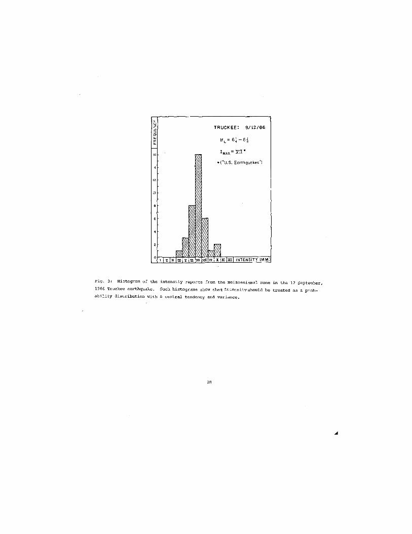
the Truckee earthquake of September 12, 1966, is given in Figure 3, If only the maximum in­

tensity recorded was used, then this earthquake would be given a maximum intensity of X,

based on landslides; if the mean intensity was used then VII is appropriate. The former

radical bias was not the procedure followed by the USC&GS, and more recently by the USGS, in

preparing intensity summaries for United States earthquakes. If the correlations between

peak acceleration and intensity are to be used for quantitative purposes as a basis for engi­

neering design, then a more appropriate statistical model must be used in making the regres­

sions between the parameters. It should be added that the same error has arisen in regress­

ing the logarithm of the fault rupture length in earthquakes to their magnitudes. This for­

mula is also used in site evaluations to determine the likely design, earthquake magnitude,

and ultimately the peak acceleration for a site. Regressions have been made assuming the

independent variable to be error-free, an assumption which is clearly false so far as ob­

served rupture lengths are concerned. (See Figure 4)

27

>­u z w ::;)

o W 0:: U.

16

14

12

10

TRUCKEE: 9/12/66

• ("U. S. Earthquakes")

Fig. 3: Histogram of the intensity reports from the meizoseismal zone in the 12 September,

1966 Truckee earthquake. Such histograms show that ~ntensityshould be treated as a prob­

ability distribution with a central tendency and variance.

28

" ~ :Ii

'3 ;;;

! ~

'" =>

~ '" ~ u

i ... o

1000,--,----,--,-----,----,---,-,-,

STRIKE- SLIP FAULT DATA

~ 10~----------.r~-~---------i

~

Fig. 4: Regression l~nes for world-wide data of surface fault rupture and magnitude of the

associated earthquake~ The order of increasing slope, the lines are (a) regression of log L

on M; (b) regression of M on log L assuming L has some error (dashed line); and (e) regres­

sion of M on log L treating L as error-free. Curves (a) and (e) are from Mark and Bonilla

(1977) •

29

MODELING OF NEAR-FAULT MOTIONS

David M. Boore

Stanford University

Stimulations of strong motion accelerograms using uniform, smoothly propagating disloca­

tions in a homogeneous half-space give records that are much too simple compared to the real

thing. To some extent this may be remedied by the inclusion of layering in the system, but

we suspect that a significant degree of randomness is characteristic of the real physics of

the source process and will have to be incorporated into realistic source models, at least

for proper representation of the high-frequency end of the spectrum. Several lines of work

are underway:

Rupture Incoherence and Directivity

computed motions are often sensitive to rupture propagation because of destructive inter­

ference of the radiated waves. The interference is particularly strong for low rupture velo­

cities at azimuths away from the direction of fault rupture. These directivity effects are

present in all theoretical computations, and if real, clearly have a first order effect on

the computed near fault motions. These effects are usually predicted from smooth, coherent

ruptures; since we feel that this coherence can be destroyed by irregularities either in

fault propagation or in the elastic parameters in the material surrounding the fault (Brune,

1976, Nur, 1978), the question arises as to the effect of this incoherence on the directivity

of the radiated waves from a fault in which rupture velocity and fault slip had statistical

distributions along a fault with segments of random length was devised. This analytic ex­

pression was checked against Monte Carlo simulations. Figures 1 and 2 show some of the re­

sults. We found that the rupture incoherence can increase the high frequency motions, as has

been pointed out by a number of other authors (e.g. Aki, 1967, 1972; Haskel, 1964, 1966; Das

and Aki, 1977), and that the azimuthal and rupture velocity dependence of directivity still

exists, and in fact can be enhanced by the incoherent faulting.

.01

.001

.01

v~1.8/3.2

d~I.O/I.O

--,..". e ~ 0 0

~ .. f~0.5 ~ ··.,.>t~1.0 w-,

10

FREQUENCY, Hz

100 1000

Fig. 1: The influence of coherence length on the

mean spectrum for the fault with random variations

of rupture velocity between 1.8 and 3.2 km/sec.

Note the flattening of the spectrum due to the in­

crease of the corner frequency associated with the

coherence length.

30

Fig. 2: The mean spectra calculated

for forward and back azimuths and three

types of faulting: smooth, coherent

faulting with 2.5 km/sec rupture velo­

city and fault flip of 1.0 units; vari-

able rupture velocity ("v vary") with

upper and lower limits of 3.2 and 1.8

km/sec, respectively; and variable

fault slip ("d vary") between limits of

0.25 and 1.75 units. In the latter two

cases the mean of the fault properties

was the same as for the smooth rupture.

Rupture length was 30 km and coherence

length was 1.0 km. A shear velocity of

3.3 km/sec was assumed. Ordinate is in

arbitrary units.

A Statistical Simulation Model

1.0,-----_

0.1

1.0 _ 1/2

(E)

0.1

0.01

0.001

.01

d vary

v vary

smooth

.1 I 10 100

FREQUENCY, Hz

1000

~ preliminary study of the 1952 Kern County earthquake showed that a multisegrnent fault

would generate realistic looking strong motion records (Figures 3 and 4). In this example

the segments were chosen to approximate a smooth rupture, and it was only the small mismatch­

es between segments that produced the complicated motions. This led to the idea of a simula­

tion model based on a complex fault with randomly varying properties (this is an extension

and improvement of the model proposed by Rascon and Cornell, 1968). The experience gained

fr.om the previously discussed study of rupture incoherence has been incorporated into a first

generation form of such a simulation model. An example of a simulation of the accelerogram

recording at Temblor during the 1966 Parkfield, California earthquake (see Figure 5 for the

geometry) is shown in Figure 6. In this Figure we compare the data (top) to a smooth rupture

and to ruptures with mean velocities of 2.5 and 2.9 km/sec which start at the epicenter and

propagate southeast to a point somewhat beyond Gold Hill. The bottom trace shows the motion

from a unidirectional rupture starting near Gold Hill and propagating along the fault away

from Temblor. As expected directivity effect is pronounced. Adding a small amount of rup­

ture to the southeast would have increased the amplitude (but not the duration) of this re­

cord.

31

5

Fig. 4: Comparison of waveforms for the Pasadena

recording of the Kern County earthquake.

",EPICENTER

\"~ARKFIELD , ,

\ '\:0 HILL ,

o 5 KM \'" '---' " eTEMBLOR , ,

"-"\

"-32

Fig. 3: Schematic of 1952 Kern County

earthquake rupture surface. Rupture

started at the left side.

~ 5[ w ~o

5 -5

b 10 (seconds)

Fig. 5: Geometry of Parkfield simula

tion.

Fig. 6: Simulation of Temblor recording with a

complex fault.

Surface Waves in Strong Motion

Temblor

Smooth Rupture

V=2.5km/5ec

V=2.9 km/sec

Rupture away

o 10 sec ~,~~~~~

r59

o

Moving away from the generation of high frequencies by complex faults, at lower fre­

quencies geologic structure can have an important influence on the motions; and for ground

displacements in particular, the dominant motions may be best described as surface waves.

We are investigating the simulation of these types of motions using straightforward modal

superposition. There are many adv~ntages to this technique: an almost arbitrarily compli-

cated layered structure can be used; P and SV type motion is as easy to generate as Sh

motion and all multiple bounces are included (this is not true of the often used Cagniard-

de Hoop technique); simulations for any source type (including propagating sources of finite

width) and distance are very inexpensive to simulate once the dispersion parameters are cal­

culated -- and these can be quickly evaluated using existing programs. Figure 7 shows an en­

couraging comparison between data (top), the complete solution for a multilayered half space

(middle, taken from Heaton and Heimberger, 1978), and our surface wave solution (bottom).

The modeling of existing data is about the only means we have of estimating the physical

properties of the faulting process (such as effective stress and rupture velocity). If the

multitude of studies of the Parkfield records is at all representative, there may be more un­

certainties in the derived fault parameters of various earthquakes than is usually acknowl­

edged. The problem is that these parameters are then accepted as being valid and used in the

33

derivation of subsequent parameters--after awhile one wonders what to believe. For example

in a recent attempt to survey the literature for determinations of rupture velocity (which

seems to have a first order effect on ground motions), I came across a table in which rup­

ture velocities of 2.3 km/sec and 3.5 km/sec were the most common entries: on closer exam­

ination almost all of these values were taken from the papers of one researcher. To illus­

trate the nonuniqueness, I repeated one of the waveform simulations using a velocity of 3.2

km/sec and a larger rise time to make up for the sharpening of the pulses due to the faster

propagation velocity. The result in Figure 8 speaks for itself. (Interestingly, the tabula­

tor pointed to this particular earthquake as one for which the rupture velocity was well con­

strained. )

The point I'm raising is that if we are to use parameters from past earthquakes to guide

our simulation of ground motions, a critical reevaluation of these derived parameters may be

necessary.

OATAf\_ ;1 di _ r ~j~-IAV~I~~V :!. ,fl···: /

,'I 2

TIME (sec)

Fig. 8,

SUM

FIFTH

FOURTH

34

Fig. 7: Data and synthetics for the transverse

component of the IVC recording of the Brawley

earthquake, 11-4-76. The range is about 33 km

and the source depth is about 7 km. Data and

Cagniard synthetic are from Heaton and HeIm­

berger (1978). {The dashed line is the Cagniard

solution.}

I.

I I

I ,

f\ ~ (Kanamori,1972) \ Rise time= 3.0 sec

\ V :: 2.3 I<mfsec

REFERENCES

Aki, K., Scaling law of earthquake source time function, Geophys, J. R. astr. Soc., 31, 3-25,

1972.

Brune, J. N. The Physics of earthquake strong motion, ch. 5 in Seismic Risk and Engineering

and Engineering Decisions (C. Lomnitz & E. Rosenblueth, ed.), Elsevier Scientific Publ.

Co., Amsterdam, 140-177, 1976.

Das, S. and K. Aki, Fault plane with barriers: a versatile earthquake model, J. Geophys. Res.

82, 5658-5670, 1977.

Haskell, N. A' I Total energy and energy spectral density of elastic wave radiation from pro­

pagating faults, Bull. Seism. Soc. Am. 54, 1811-1841, 1976

Haskell, N. A" Total energy and energy spectral density of elastic wave radiation from pro­

pagating faults, Part II. A statistical source model, Bull. Seism. Soc. Am. 56, 125-140.

Heaton, T. H. and D. V. Helmberger, Predictablility of strong ground motion in the Imperial

Valley: modeling the M 4.9, Nov. 4, 1976 Brawley earthquake, Bull. Seism. Soc. Am.,

1978, (in press) .

Nur. A., Nonuniform friction as a physical basis for earthquake mechanics: a review, subm. to

Pure and Applied Geophysics., 1978.

Rascon, o. A. and C. A. Cornell, Strong motion earthquake simulation, MIT School of Engr. Res.

R-68-15, 155 pp., 1968.

35

A DYNAMIC SOURCE MODEL FOR THE SAN FERNAtmO EARTHQUAKE

Michel Bouchan

Massachusetts Institute of Technology

We present a study of the rupture mechanism of the San Fernando earthquake. In the near­

field we model the earthquake as a two-dimensional propagating rupture in a half-space. We

synthesize the strong ground motions and accelerations at the Pacoima Dam site using the dis­

crete horizontal wave number method of Bouchon and Aki (1977). We take for the slip-time­

history on the fault plane analytical expressions which approximate the slip functions of

dynamic crack models obtained by Das and Aki (1977, 1978). These models allow for the pre­

sence of barriers or obstacles on the fault plane. Such barriers are made of high-strength

material and may remain unbroken after the passage of the rupture front. Their presence re­

sults in a strong enhancement of the high-frequency radiation. This can be seen in Figure 1

where the velocity waveforms synthesized at the Pacoima Dam site and radiated by the upper

part of the fault for a uniform dislocation model (A) and for a crack with barriers model (B)

are compared. Two major features of the Pacoima Dam accelerograms--the strong pulse associ­

ated with the beginning of the rupture, and the high-acceleration phase which arrives in the

middle of the records and lasts almost until the end of the disturbance--which are not com­

patible with a smooth rupture process are well explained by a crack with barriers model. An

example of synthesis of the ground acceleration at the Pacoima Dam site is shown in Fig. 2.

)0-.... e::; o ...J ... >

...J

~ Z o N it: o J:

A

o 2 4 6 TIME (SEC)

36

Fig. 1: R indicates the Rayleigh wave radi­

ated by the upper tip of the fault.

I" ':',..+ '-"~~~MI\~'~1 I:'

Fig~ 2: Horizontal (A) and vertical (B) accelerograms synthesized at the Pacoima Dam site

for a crack with barriers model. The beginning of the accelerograms corresponds to the

arrival of the P-wave from the hypocenter. The shear wave radiated from the hypocenter (S)

and the Rayleigh wave generated at the upper tip of the fault (R) are identified. The cut­

off frequency is 10 Hz and the total length of the signal is 9.6 sec.

The P wave shortperi:od teleseismic records are characterized by a high amplitude-short

duration first pulse indicative of a massive and localized initial rupture (Hanks, 1974). We

model this initial rupture event as an expanding circular shear crack stopping suddenly. A

comparison of the calculated pulse with the data yields a value of the source radius of the

initial rupture event of about 1.5 krn and a stress-drop on the order of 500 bars. This indi­

cates a high level of tectonic stress in the region. A rectangular fault with randomly dis­

tributed barriers is used to model the rest of the rupture process at teleseismic distance.

Such a model produces ripples on the seismograms, quite similar to the ones present on the

records.

A study of the earthquake series following the main shock shows that the aftershocks

which take place in the region where major slip occurred during the earthquake may represent

the release of some of the barriers.

Our interpretation of the rupture process is the following: the earthquake starts with

a massive and localized initial rupture indicative of a high tectonic stress. The l~ited

areal extent of this initial rupture shows the presence of barriers of very high strength in

the hypocentral region. Skipping these barriers, or partially breaking them, the rupture pro­

gresses mostly upwards, encountering a large number of barriers of small areal extent which

offer a strong resistance to the propagation of the rupture.

REFERENCES

Bouchon, M. and K. Aki, Discrete wave-number representation of seismic source wave fields,

Bull. Seis. Soc. Am., 67, 259-277, 1977.

Das, S. and K. Aki, A numerical study of two-dimensional spontaneous rupture propagation,

Geophys. J. Roy. astro. Soc., 50, 643-669, 1977.

37

DaS, S. and K. Aki, Fault plane with barriers: a versatile earthquake model, J. Geophys. Res.

1978, (in press) .

Hanks, T. C., The faulting mechanism of the San Fernando earthquake, J. Geophys. Res., 79

1215-1229, 1974.

38

ALTERNATIVE GROUND MOTION INTENSITY MEASURES

C. Allin Cornell

Massachusetts Institute of Technology

There are reasons to consider alternatives to peak acceleration (or velocity or M. M.

Intensity) as scalar measures of ground motion intensity. In particular an ordinate of the

Fourier amplitude spectrum of acceleration (at, say 1 hz) suggests itself, see Figure 1. We

study this (and other) alternatives, first, as they function as predictors of structural re­

sponse, and, second, as they can be predicted from typical event variables (magnitude, M, and

hypocentral distances, R). Together the "errors fl (statistical dispersions) in these two pre­

dictions determine how well structural response can be predicted from M and R (via a scalar

intensity measure, see Figure 2).

We compare, too, peak acceleration alone as it can be predicted directly from distance

and M. M. epicentral intensity, IO' versus its prediction from Rand IO via magnitude or via

M. M. site intensity. There are biases in the latter two paths, paths which may be necessary

in regions where strong motion data is effectively non-existant, see Figure 3.

1.4

C.O.v 1.2 ' .......

-~

C 1.0 0

B .;:: 0 > 0.8

a c 0.6 Sv Q) :g Dp ----Q) 0.4 ~ 0 U • FS(O.3)

0.2

2 % Damping

'i: 'i:

" " " " " "

Fig. 1

" "

39

/ /

/ (/

Natural frequency

280

240

'" 200 u Q)

-!( E 160 u

c:i: <I 120

80

40

0 0

A

C

\D \ \ \ \ \ ,

\ \ , , , , , ,

"

A

D

c

" '"

R, km

Fig. 2

Fig. 3

40

---------

LET I S BE MEAN

Neville C. Donovan

Dames & Moore

These notes and attachments are intended to provoke discussion, but must at the same

time be accepted as my own personal viewpoints. These views probably disagree with those of

other workshop members, and if so, useful discussion should ensue.

The first point I would like to make is a plea that we make an effort to move away from

a fixation on the search for a maximum of peak quantities associated with earthquakes. In­

stead of the premise that the peak instrumental relationship is a function of the number of

instruments deployed, we should recognize the simple statistical expectation that as the

sample gets larger, the expectation that a larger value will be obtained increases. Fortun­

ately, while we chase around looking for the extreme, we obtain a mean value that becomes in­

creasingly reliable and we gain more information about the scatter of the data values about

the reliable mean. From the statistical point of view the Pacoima Dam record is not of

special interest. If we carefully keep track of mean values together with the statistics

related to the distribution about the mean, we are proceeding in a fashion analogous to fol­

lowing the center of the road while at all times knowing how wide the road is. Other pro­

cesses lead to either an unknown position on this road, which might even approximate a random

walk, or an attempt to follow the indeterminate yet precipitous edge.

How we handle the data we have is also important. There are many ways that established

routine processes can bias data. Bollinger showed this first, but I would like to demonstrate

it also with an example where all the hard work was done by others.

The event which occurred in Washington State on December 14, 1872, has attracted a lot

of interest through its importance to nuclear power plant siting. A study supported by a

group of utilities in the pacific Northwest supplied intensity values for specific sites and

intensity isoseismals. The usual pattern of an isoseismal map is familiar, so I would like

instead to show the data in terms of Figure 1, where individual values are plotted as small

circles and the equivalent isoseismal radius value is plotted as a triangle (isoseismals

could be well approximated by a circle). The biasing produced by drawing isoseismals is read­

ily apparent by comparing the circles and the triangles positions, but let us do some least

squares fitting. Figure 2 shows the separate best fits to individual points and equivalent

radii and demonstrates that the bias in the equivalent radii method is about 3/4 of an inten­

sity--hardly a mean!

The tables attached show the difference between the mean and the value one standard de­

viation larger computed by several different investigators for three parts of the strong mo­

tion problem. These are: (1) peak acceleration, (2) velocity to acceleration ratios, and (3)

special amplification values. If one is to follow, as is often suggested, the practice of a

value one standard deviation larger than the mean value, the end spectral values could be

41

VIII~'\

~ INDIVIDUAL SJTES

I'~ . . EQUIVALENT RADIUS FROM

'I~ ~ . EX~S:::~:~~O~~NESHOWN DIOTTED

.. - .... _ ..... I I I I ~I .. ~ ~~ FROM EQUIVALENT Rt'

···~)..~·I \ FROM INDIVIDUAL POINTS "" .......... __ .

>-~ VII

VI

DECEMBER 14,1872 LAKE CHELAN, WASHINGTON

LEGEND: Fig. 1: Individual MM Intensity

versus distance data points de­

rived from historic descriptions

for December 14, 1872 Washington

state earthquake and Intensity

versus distance values obtained

from isoseismal map_

/~.l "'''''- I . . '" ., '" -'-. " I -T--

"',. I' IV

III

"0 loa 200 300 400 EPICENTRAL DISTANCE IN

Fig. 2: Lines based on least

squares fit showing the bias to at-

500 60a KILOMETERS

VIII

VII

tenuation estimate when the quiva- VI

lent isoseismal radii are sued in-

stead of individual MM Intensity

values obtained from felt report

distance. IV

III

700 800

, BIAS (AVERAGE: 0.73 UNITS TO 500 KILOMETERS)

I

FROM EQUIVA'LENT RADII

I I I ~CM INDI1VIDUAL P01INTS

I "-__. I __.

-1--

"0C----:,C:c0=---2:-'0,.,0--3'"0-0--4--'0-,-0--5""0-0--6-'-OO---70'--0--..J800

EPICENTRAL DISTANCE IN KILOMETERS

42

more than four times larger than the most probable value. Surely we have a need for knowing

both where the middle of the road is and how wide it is.

Although much research has been done, the scientific and engineering fraternities are

still unable to predict ground motions with any precision. The recorded motions from the

Humboldt Bay Nuclear plant and site response studies have been used as the basis for a Type

A (before the fact) prediction claim by using the free-field values to compute motion levels

inside the structure. The full prediction, however, would also require information regarding

the free-field motions which the present state of our knowledge is unable to do. Figure 2

shows what happens with attempts to predict the peak acceleration. All fall grossly short of

the observed motion and show that Type A claim is only valid when a substantial part of the

problem answers are known in advance. The choice of peak acceleration for this example waS

made for convenience. The actual choice of parameter for comparison is relatively minor. I

do recommend that some other parameter than peak acceleration be more widely used and dis­

cussed. Maybe we should directly measure something else!

(!)

I- 30 i'5 () a: ~ , is 20

~ a: w ...J W

8 10 <t ~ <t w a.

SCHNABEI:SEED(l973) M=5.6 a

STORAGE BLDG • . -:.> HORIZONTAL

"'"' C?-REACTOR BLDG. ... •

•

°O~~--~--L-~---L--~~ 20 40 60

KILOMETRES

Fig. 3: Instrumental peak acceleration values recorded during the June 7, 1975 Ferndale

Earthquake (Magnitude approximately 5.5 with a 20 kilometer focal depth).

43

TABLE 1

Estimates of Uncertainty

Author

a) accerleration Esteva 1970 Esteva & Villaverde 1973 Donovan* 1973 Donovan 1973 Donovan & Bornstein** 1975 Seed et a1*** 1976 McGuire 1974

b) velocity Esteva 1970 Esteva & Villaverde 1975 McGuire 1974

c) displacement McGuire 1974

San Fernando data only

" Site specific relationship ***Seed,et;.al data are sorted by site characteristics

and consider only one magnitude level

TABLE 2

standard Deviation Lognormal

1.02 0.64 0.48 0.71

0.3 -*0.5 0.34-*0.51

0.51

0.84 0.74 0.63

0.76

Ground Motion Parameter Ratios

via via via via

Newmark-Hall Seed et al Mohraz

Profile Type cm/sec/g cm/sec/g cm/sec/g L' S'

Rock 61(24)** 66(26) 61 (24) 69(27)

Stiff Soil 114 (45)

Peep Sand 140(55) 76(30) 91(36)

Alluvium 122(48) 122(48)145(57)

Factor

2.8 1.9 1.6 2.0

1.3->-1. 7 1.4-*1. 7

1.7

2.3 2.1 1.9

2.1

Standard Deviation

Factor Mohraz

L S 1.58 1.63

1.53 1.61

1.44 1.49

* Mohraz considered horizontal data in two sets. L comprises the set containing the largest horizontal component from each site and the S set contains the lower value.

**Numbers in parentheses are in units of inches/sec/g.

44

TABLE 3

spectral Uncertainty

Averaged Across Spectra Damping Level Blume-Newmark Mohraz Seed et. a1

Average 1.42 1.41

1.37 1.36 1.4

1.30 1.31

REFERENCES

Donovan, N. C., A statistical evaluation of strong motion data, including the February 9,

1971 San Fernando earthquake, proceedings of the Fifth World Conference on Earthquake

Engineering Rome, Itly, 1252-1261, June 1973.

Donovan, N. C. and A. E. Bornstein, A review of seismic risk applications, second Inter­

national Conference on Applications and Statistics and Probability in Soil and Struc­

tural Engineering, Aachen, vo.l. III, 1975

Esteva, L., Seismic Risk and Seismic Design Decisions, Seismic Design for Nuclear Power

Plants, The MIT Press (edited by Robert J. Hansen), Cambridge, Massachusetts, 142-182.

1970.

Esteva, L. and R. Villaverde, Seismic Risk, Design Spectra and Structural Reliability,

unpublished report University of Mexico, 1973.

Hall, W. J., B. Mohraz and N. M. Newmark, statistical Studies of Vertical and Horizontal

earthquake spectra, prepared for the United States Nuclear Regulatory Commission, NUREG-

003, January, 1976.

McGuire, R. K., Seismic Structural Response Risk Analysis, Incorporating Peak Response Re~

gressions on Earthquake Magnitude and Distance, School of Engineering, Massachusetts

Institute of Technology, Cambridge, R74-51 Structures Publication 99, 1974.

Mohraz, B., A Study of Earthquake Response Spectra for Different Geological Conditions, Bull.

Seism. Soc. Amer., 66, No.3, 915-935, June 1976.

Newmark, N. M. and W. J. Hall, Seismic Design Criteria for Nuclear Reactor Facilities, Pro­

ceedings of the Fourth World Conference on Earthquake Engineering, Santiago, Chile,

Vol. II, B4 37-50, 1969.

Seed, H. B., C. Ugas and J. Lysmer, Site Dependent Spectra for Earthquake-Resistant Design,

Bull. Seism. Soc. Amer., 66, No.1, 221-255, February 1976.

Seed, H. Bo, R. Murarka, J. Lysmer, and I~ M. Idriss, Relationships between Maximum Accelera­

tion, Maximum Velocity, Distance from Source and Local Site Conditions for Moderately Strong Earthquakes, Bull. Seism. Soc. Amer., 66, No.4, 1323-1342. 1976.

45

MEASURES OF HIGH-FREQUENCY STRONG GROUND MOTION

Thomas C. Hanks

united states Geological Survey

Since the first strong motion accelerograms were written more than forty years ago,

peak acceleration has been the most commonly used, single index of strong ground motion. It

has, however, been known for some time that peak acceleration need not be-~and too often can­

not be--a uniformly valid measure of strong ground motion over the entire frequency band and

amplitude range of engineering interest. The very character of the peak acceleration datum

as a short period, time-domain amplitude measurement is the principal reason for two impor­

tant limitations on its value as a measure of strong ground motion. First, for M ~ 5 earth­

quakes at close distances, taken here as a rough threshold of potentially damaging ground

motion, the period of this phase is much shorter than the faulting duration. Thus the peak

acceleration simply cannot measure gross source properties of potentially damaging and des­

tructive earthquakes, even if such data may, in a large enough set of observations, indicate

limiting conditions on the failure process in very localized regions of the fault surface.

Secondly, this same characteristic of the peak acceleration datum makes precise corrections

for wave propagation effects, including anelastic attenuation and elastic scattering, impos­

~ible except under very unusual conditions. Both of these problems, but especially the

second, are in turn responsible for the notoriously large scatter in peak acceleration data,

even through very small variations of magnitude, distance, and site conditions. And it is

this last problem that limits the utility of peak acceleration even as a measure of high­

frequency strong ground motion.

These difficulties in interpreting, manipulating, and using peak acceleration data are

widely acknowledged, I believe, by investigators of strong ground motion, whether they be en­

gineers or seismologists. My own interest in these problems has arisen in connection with

recently acquired peak acceleration data at small magnitudes (M ~ 5) and close distances

(R ~ 10 km) (Hanks and Johnson, 1976; Seekins and Hanks, 1978), and in those studies we have

discussed these issues extensively. But none of that discussion is particularly informative

about the really important issue: if peak acceleration is not a reliable measure of high­

frequency strong ground motion, as is generally agreed to be the case, then what is? In this

correspondence,' I will suggest such a measure based on simple earthquake source models that

indeed seems better than peak accelerations and perhaps might be.

Simple displacement spectral models of the far-field shear radiation of earthquakes are

specified by the long period level, Qo

' proportional to seismic moment, Mo' the corner fre­

quency, fa, proportional to reciprocal source dimension, f, (or reciprocal faulting duration,

Tdl and high-frequency' (f > fol spectral decay of the form (f/fol-Y. A variety of observa­

tions, including ~-Ms data, peak accelerations as a function of M at R ~ 10 km, the wealth

of observations for the San Fernando earthquake (at frequencies as high as 100 x fo)' as well

46

...

as single station spectral determinations for a large number of earthquakes, suggests that the y = 2 model is the one generally, although certainly not always applicable, at least in

the frequency band of engineering interest (e.g., Aki, 1967; Berrill, 1975; Tucker and Brune,

1977; Hanks, 1978).

Figure 1 presents the acceleration spectral amplitudes for the y = 2 case for far-field

shear waves for two earthquakes at the same R in the presence of anelastic attenuation. The

two earthquakes have been assigned the same stress drop ~a; in the Qo-fo notation of Hanks

and Thatcher (1972). This means

since

106 RIl f3 P 0 a

(1)

(2)

where p density. The anelastic attenuation of spectral amplitudes is taken to be of the form

exp(-~fR/QS), where f is frequency, S is shear-wave velocity, and Q is specific attenuation.

In Figure 1, f max is the frequency where the argument of the exponent is 1. Then one, non

unique interpretation of Figure 1 is that the corresponding acceleration time histories are

band limited (fa ~ f .::. fmax

)' finite duration (0':" t-R/S'::' Td), white noise. The whiteness

arises from the constant acceleration spectral amplitudes equal to Qof~ in the band

fo < f < f , but the randomness has simply been assumed. - - max

The idea that ground acceleration time histories can be taken as band limited, finite

duration, white noise is a reasonable one in view of the generally chaotic nature of strong

motion accelerograms in finite time windows and frequency bands for M ~ earthquakes. Indeed,

this same notion has been the basis for considerable work in the analysis of existing acceler­

grams and in the computation of synthetic accelerograms for more than 30 years in the engi~

neering community (e.g. Housner, 1947; Hudson, 1956; Bycroft, 1960; Housner and Jennings,

1964; Jennings et al., 1968). It is a pleasure to welcome these investigators to the com­

munity of y = 2 proponents, at this however belated date.

In any event, the root-Mean-square acceleration arms of the acceleration time history

corresponding to the acceleration spectra in Figure 1 can be obtained through an application

of Parseval's Theorem:

*In source mechanism parlance the expression "high .... frequency" means freque:ncies greater

than the corner frequency, but in the sense of structural engineering, this expression gen­

erally means vibrations at frequencies of several Hz or greater, In this study we are using

"high-frequency" in the former sense. Since corner frequencies of M ft, earthquakes are less

than 1~2 Hz, the engineering sense of this expression is contained within the seismological

one used here.

47

(3)

where aCt) is the acceleration time history, ~(W) is its Fourier amplitude spectrum, and

w is circular frequency. Ignoring contributions outside the ranges 0 ~ t-R/S ~ f ~ f rnax ,

we write (3) as

The rms acceleration is

a rms

Equations (2) and (3), together with

and

result in

a(w)

f o

a rms

a rms

1 Td

1 Td

2'1ff

! maX!2

ii(w) dw

1/2

Qo(f 2'1f)~ f < f < f o 0- -max

12 (2'1f) 2 f:,a

102 pR

f max f

o

(4)

(5)

(6)

(7)

(8)

Table 1 compares arms values estimated from (8) with those "observed" for the San

Fernando earthquake at Pacoima Dam and the Kern County earthquake at Taft. The "observed"

values are those given in Volume I of the series "Strong Motion Earthquake Accelerograms I"

corrected by (record length/Td)1/2 to estimate the (larger) a value that occurs in the rms

time interval of the S-wave arrival through the S-wave arrival plus Td" Because the accel-

erations are non zero outside of this interval, the "observed If values are overestimates of

the actual arms values, Q ~ t-R/S 2 Td" In any case, however, the agreement between the

estimated I and "observed" values is remarkable, by conventional seismological standards, in

estimating high-frequency amplitudes, being approximately 50% in the case of the San Fernando

48

..

earthquake and 20% in the case of the Kern County earthquake.

Logo at R

Fig. I: Far-field shear wave acceleration spectra at R for two constant stress drop earth­

quakes.

Table 1

Comparisons of Estimated and Observed arms Values

San Fernando Earthquake

Feb. 9, 1971, ML = 6.4

1026

dyne-em

10 Jan

50 bars

0.1 Hz

at Pacoima Dam

10 Jan

25 Hz

140 em/see2

220, 240 cm/see2

M o

r

11o

f o

R

f max

a rms

estimated

I'observed II

Kern County Earthquake

July 21, 1952, M = 7.7

2 x 1027

dyne-em

25 km

60 bars

(0.04 Hz)

at Taft, California

40 Jan

Hz

36 cm/see2

42, 42 em/sec2

There is nothing new in the suggestion that arms is an important index of strong ground

motion nor in the recognition that arms is related to the spectral amplitudes of ground mo­

tion, specifically through (3) and (5). The point I wish to emphasize is that arms can also

be related to physical parameters of the gross faulting process and source-station path,

through (8). Thus, empirical correlations of arms with other physical variables can be set

within a theoretical or predictive framework, which in turn can be used to estimate arms

49

(and therefore spectral amplitudes of high-frequency strong ground motion) in the absence

of any ground motion observations, provided one can realistically choose ~a, £0' Rand Q

for the source-station combination of interest.

Even so, the only really important issue is how well this measure of high-frequency

strong ground motion works, in both an observational and theoretical sense. Observationally,

the issue is whether or not arms determinations obtained from ground motion time histories

show less scatter than peak accelerations for the same set of other variables, specifically

M, R, and site conditions. Theoretically, the issue is whether or not we can predict, to

the desired level of accuracy the observations in terms of ~a, fa, R, and Q with appropri­

ate allowance for site conditions. The remarkably good agreement between the estimated and

"observed" arms values for the two important accelerograms discussed earlier is encouraging

in the latter connection, but considerably more effort must be devoted to both issues. The

Oroville aftershock accelerograms appear to be a particularly valuable resource for these

investigations. Finally, since (7) and (8) are built on the far-field representation of the

y = 2 model, it can be expected to fail close enough to a large enough shock, unless we speci­

fically account for the near-field effects that can (but need not) affect periods of a second

or so and longer. Otherwise we would be clever enough to break big earthquakes into small

enough analytical chunks.

REFERENCES

Aki, K., Scaling law of seismic spectrum, J. Geophys. Res., 72, 1212-1231, 1967.

Berrill, J. B., A study of high-frequency strong ground motion from the San Fernando earth­

quake, Ph.D. Thesis, California Institute of Technology, Pasadena, 1975.

Bycro£t, G. N., White noise representation of earthquakes, J. Engg. Mech. Div. ASCE, 86,

1-16, 1960.

Hanks, T.e., b-values and w-Y seismic source models, Proceedings of Conference III - Fault

Mechanics and its Relation ot Earthquake Prediction, Office of Earthquake Studies, u.s.

Geological Survey, Menlo Park, Calfiornia, 1978

Hanks, T. C., and D. A. Johnson, Geophysical assessment of peak accelerations, Bull Seismol.

Soc. Amer., 66, 959-968, 1976.

Hanks, T. C., and W. R. Thatcher, A graphical representation of seismic source parameters,

J. Geophys. Res., 77, 4393-4405, 1972.

Hausner, G. W., Characteristics of strong-motion earthquakes, Bull. Seism. Soc. AIDer" 12, 19-31, 1947.

Housner, G. W., and P. C. Jennings, Generation of artificial earthquakes, J. Engg. Mech. Div.

ASCE, 90, 113-150, 1964.

Hudson, D. W., Response spectrum techniques in engineering seismology, World Conference on

Earthquake Engineering, Berkeley, California, 1956.

Jennings, P. C., G. W. Housner, and N. C, Tsai, Simulated earthquake motions, Earthquake

Engineering Research Lab., California Institute of Technology, Pasadena, California. 1968

so

Seekins, L. c~, and T~ c. Hanks, Strong motion accelerograms of the Oroville aftershocks

and peak acceleration data, Bull. Seism. Soc. Amer~, in press, 1978.

Tucker, B. E., and J. N. Brune, Source mechanism and ~-Ms analysis of aftershocks of the

San Fernando earthquake, Geophsy. J. R. Astr. Soc., 49, 371-426, 1977.

51

SYNTHESIS OF SAN FERNANDO

STRONG-MOTION RECORDS

Thomas H. Heaton and Donald V. HeImberger

Seismological Laboratory

California Institute of Technology

Three-dimensional models of a finite fault located in a balf-space are constructed to

study the ground motions from the 9 February 1971 earthquake as observed at JPL, Palmdale,

and Lake Hughes (Array Station #4). The Cagniard-De Hoop Technique is used to compute the

ground motions due to infinitesimal point sources which are evenly distributed (0.5 km

spacing) on the fault plane. The responses are summed with time lags determined by the

assumed hypocentral solution and rupture velocity. Nonuniform fault displacement is

modeled by varying the weights of individual point sources. By investigating the motion

due to small sections of the fault it is possible to understand how various wave types

interfere to produce the motion due to the total fault. Recent modeling of teleseismic

body waves by Langston has indicated that the fault changes dip from 500 to 300 at a depth

of approximately 5 km. This feature has been incorporated into our models. The assumed

fault geometry and station locations are shown in Figure 1. In Figure 2, we display

assumed fault displacements for a preliminary moqel which is used to explain the motions

at JPL, PLM, and LKH. The overall moment for this model is 1.5 x 1026 ergs. The hypo­

center is assumed to lie in the region of maximum displacement and a rupture velocity of

1.8 km/sec (as suggested by Langston) is also assumed. Although stations LKH and JPL are

situated at roughly equal epicentra1 distances, there appears to be a dramatic difference

in the character and amplitUdes of ground motion seen for these stations. This can be

seen in Figures 3 and 4. In these figures, the synthetic ground motions for the fault

model described above are compared with the integrated accelerograms for these stations.

Because the integrated acce1erograms have been filtered with an 8 sec. Ormsby filter, the

synthetics are displayed both with and without the inclusion of this filter. Although it

appears that the particular fault model used for Figures 3 and 4 is not, in detail, correct/

it does well at explaining the differences in character and amplitude of ground motions as

seen between JPL and LKH. An examination of Figure 5 helps one to appreciate the complex

interplay between source and wave propagational effects. In this figure the fadlt is

subdivided into 5 strips each of which has a width of 4 km. Also shown are synthetic

motions (JPL, North) for a single point source located in the middle of each subfault.

Although these point sources produce easily interpreted specific arrivals, it is clear

that the JPL record results from complex and not easily interpreted interaction of both

source and propagation effects. These synthetics also demonstrate the dramatic effect

of the free-surface. Rayleigh wave and sP head wave contributions are of great importance.

52

The effects of even more complicated earth structure in these records is yet to be studied,

but detailed synthesis of records for simpler aftershocks should add some insight to this

problem.

eLKH Lake Hughes

Circular Rupture --... Front

2km

'------_.

epLM Palmdale

Assumed Fault Shape

-... Hinge Line

""-- Approx. Surface Rupture

o 5 10 km

Fig. 1: Assumed geometry for the San Fernando

Displacements given in meters

0.6

0.

..----~

~ o 2 4 km

Fig. 2: Contour map of assumed fault dis-

fault and receivers. 1 Model consists of a placements for the preliminary San Fernando

three dimensional finite fault in a half-space. model displayed in Figures 3, 4, and 5.

A Green's function technique is used to inte-

grate the exact solution for a point disloca-

tion over the rectangular grid shown. A cir-

cular rupture front propagates from an assumed

hypocenter and displacement magnitudes are pre-

scribed on the fault surface.

53

o

FS.

I.A.

5 em

Lake Hughes # 4 (LKH)

6 12 see 18

Fig. 3 and 4: Preliminary model of JPL and LKH displacement records. Massive faulting

at depth of 13 km and a rupture velocity of 1.8 km/sec. are assumed. The top trace is

the synthetic ground motion; the middle trace is the synthetic ground motion filtered

with an 8 sec Ormsby filter; and the bottom trace is the observed displacement which has

also been filtered at 8 sec. Notice the contrast between the records at JPL and LKH which

lie at approximately equal epicentral ranges.

54

Depth, km (Northj A

~ 13.0 JPL el

B 9.8 e2 C 6.7 e3 D 4.0

~ e4 --A-E 2.1 e5

SR SR S ' , " ,

~ B SP ~ P , ,

2

c -A/\ SP NP , ,

* 3

D " , 4

E ' , P SP S R .," NP 5

P- P Wave SP- S To P Head Wave NP - Near Field P Wave S- Shear Wave R- Rayleigh Wave

0 6 12 18 24 sec

Fig. 5: Decomposition of the N component of synthetic ground motion for JPL. The finite

fault is broken into 5 strips whose individual contributions are shown on the left. Re­

sponses of point sources which lie in the middle of these strips have been convolved with

both 3 sec. and 0.8 sec. triangular far-field time functions and are displayed in the

middle and on the right, respectively. By studying the point source responses, contribu­

tions of individual phases can be recognized in the synthetic for the finite fault. Notice

the complex interplay of source and wave propagational effects.

55

SH PROPAGATION IN A LAYERED HALF-SPACE

Robert B. Herrmann

saint Louis University

The formal solution of seismic wave generation and propagation by a point dislocation

earthquake source in a layered medium has been presented by Haskell (1964) and Hudson (1969).

The method assumes that the earth can be modeled by a stack of plane homogeneous layers. The

solution is obtained by performing a double integration over frequency and wavenumber of form:

u(r,~,z,t) u(k,~,z, J (kr) e- iwt dk dw • n

For a non attenuating medium, the wavenumber integration is complicated by the presence

of branch points and poles along the real k-axis. The problem can be modified through the

use of contour integration in the complex k-plane to avoid numerical problems due to these

singularities. The problem is further complicated in this case because the contour inte­

gration requires the use of the Hankel function H(2) (kr) and the modified Bessel function n

Kn(Tr). Herrmann (1977) presented a numerical solution to the SH contribution to tangential

displacements when contour integration is used. The numerical contour integration techni­

ques used provide valid results at distances as close as one-third the source depth and have

been extended to distances of 500 km and to frequencies as high as 10 Hz.

The purpose of this study is to generate realistic transverse wave time histories for

some central United States earth models in order to obtain an insight on the nature of ground

motion time histories, maximum ground motion parameters, and response spectra.

As an example of the computations, some results are given here for the simple case of a 3

single layer overlying a half~space. In the layer Sl = 3.55 km/sec and PI = 2.8 gm/cm ,

while in the half-space S2 = 4.67 km/sec and P2 = 3.3 gm/cm3

• A point vertical strike-slip

source with a seismic moment of 1.0 E 20 dyne-cm is placed at a depth of 10 km in a 40 km

thick crust p The time derivative of the dislocation time history and its corresponding

spectrum are given in Figure 1. Figures 2 and 3 show the computed displacement, velocity,

and acceleration time histories at distances of 50 km and 400 km, respectively. A low pass

filter at 1.0 Hz was used, The displacement and acceleration time histories were computed

from the velocity time history, assuming the velocity to be composed of linear segments.

Figures 4 and 5 sbow the corresponding response spectra for 0, 2, 5, and 10% damping. Of

intere$t In a preliminary interpretation is the observation that while the maximum ground

displacement, velocity, and acceleration vary as r~l OVer this distance range, the response

spectra varies as r~0,6 at certain periods, The response spectra also become more complex

with distance, just as the time histories become more complex due to the layering effects.

Herrmann (1977) showed that even a simply layered structure like this can introduce complexi­

ties in the scaling of maximum ground motion with distance due to the surface wave contri-

56

butions. Theoretical studies of this sort should provide considerable insight for the

scal~ng o~ r~al qata.

Fig. 1,

::! D2

'e '] "'" 1 0 ,

0 V2 '"

'~'] +---"~ 0 ,

<- A2 0

1, '1 '"::; ~

0 I

~ .00 ,b .00 25.00 4b .00 T - X/4.67

...

50

50

50

55.00

o

:] ~'------5.00

100

u 10-' w en

I >: u

rh.oa 55.00

10-3 ~10~-'~~~~~0~~~~

10 10' FREO (HZ)

57

~'3.~] .~

1O-4c-------,------~-----

u w (J)

"-:L 10-' u

> (J)

lL

~oo 10-6

~, -00--"'-10""""'.0"-0 -""CC. 0"'0 ---,4b'.::00,-----;,,,, .-:C00;--'1b 5. T-X/4.67

G2 R=50km

Fig. 3

u w (f)

PERIOD (SEC)

Fig. 4

10-·,r------,------r----~

"­:L 10-6e------+++¥-A.*!t,;.....--!------u

> (J)

lL

1 O-·l-----I--+-----+~----:I

G2 R=400km

PERIOD (SEC)

Fig. 5

58

REFERENCES

Herrmann, R. B., Earthquake generated SH waves in the near field and near-regional field,

Misc. Paper S-77-12, Waterways Experiment Station, Vicksburg, 94, 1977.

~askel1, N. A., Radiation pattern of surface waves from point sources in a multi-layered

medium, Bull. Seis. Soc. Am., 54, 377-393, 1964.

Hudson, J. A., A quantitative evaluation of seismic signals at teleseismic distances - II.

Body waves and surface waves from an extended source, Geophys. J. 18, 353-370, 1969.

59

STATISTICS OF PULSES ON STRONG MOTION ACCELEROGRAMS

G. W. Housner

California Institute of Technology

The strong phase of an accelerogram recorded reasonably close to the causative fault, for

example the 2/9/71 Holiday Inn record or the 5/18/40 El Centro record, has the general appear­

ance of a random function with average number of zero crossings around ten per second. Be­

tween any neighbor pair of zero crossings the area under the curve represents an acceleration

pulse, as regards to a building whose fundamental period of vibration is sufficiently long.

For example, if the pulse has an area, A, its effect on a building would be to generate an

increment of momentum mnv A, or an increment of velocity ~v = A/m, where m is the mass of

the structure and v is the velocity. Thus, an increment of kinetic energy is imparted to

the building which, in the case of a single mass structure, would be

It can be expected that a pulse of area A will have an appreciably greater effect on a build­

ing than three separate pulses each of area A/3. It is, therefore, of interest to examine

the statistics of pulse areas, particularly the occurrence of pulses of large areas.

Figure 1 shows the frequency distribution of pulse areas for the NS component of the 1940

El Centro earthquake (M ~ 7), recorded approximately four miles from the surface trace of the

causative fault. This is a normalized plot whose total area equals unity; that is, the origi­

nal histogram was divided by the total number of pulses. The largest pulse had an area that

fell between 500 and 525 mm/sec.

Figure 2 shows the frequency distribution of pulse areas for the vertical component of

the 1972 Managua earthquake. The standard deviations of vertical components are always smaller

than the standard deviations of horizontal components.

Figure 3 shows the frequency distribution of pulse areas (absolute values) for both hori­

zontal components of five strong earthquake accelerograrns. The records included are: El Centro

18 May 1940, Managua, 23 December 1972; Holiday Inn, 9 February 1971; Olympia, Washington, 18

April 1949, and Taft, California, 21 July 1952.

Figure 4 shows the corresponding frequency distribution for six less intenseaccelerograms.

The largest pulse on an accelerograrn does not necessarily have the highest value of peak

acceleration, which is another example of why peak acceleration is not a reliable measure of

intensity of ground shaking.

There are certain difficulties in formulating a completely satisfactory definition of a

pulse and relating it to the source mechanism and travel path. This makes it difficult to de­

duce information about pulse areas from first principals.

60

~ EL CENTRO SITE IMPERIAL VRLLEY.COMP~NENT SOOE '(STATISTICS OF ACC. PULSES)

__________________ 4 __ •••• ___ ~ ______________ _

flRER OF PULSE (MH/SEC.)

Fig. 1

61

~ MRNRGUR.NICRRRGUR 1972 COMPo OOWN I (STRTISTICS OF RCC. PULSES)

ISO 175 2IXJ 22S 25Q 27S 300 3:5 3SO

Fig. 2

62

~ STRTISTICS OF RCC. PULSE-RRER OF 5 LRRGE E/O (HORIlONTRL COMPONENTS ONLY)

~ ~ ~ § 0 ci ~ ci

Fig. 3 '

63

STRTISTICS aF RCC. PULSE-RRER aF 6 SMRLL E/Q CM=5-6) HaRIZaNTRL COMPaNENTS

~ 8 § § ~ ! ! .; 0 .; .; .; 0 0 .; 0 .;

100 110 120 130 ]qO ISO 160 170 180 190 200 210 220 230 2~O 250 260 270 280

ABSQLUTE PULSE -AREA( MM/SECl

Fig. 4

64

AN INTRODUCTION TO STRONG-MOTION INSTRUMENTS AND DATA

Paul C. Jennings

California Institute of Technology

INTRODUCTION

In view of the focus of the seminar upon strong ground motion, it seemed appropriate to

include in the proceedings a summary of the present status of strong-motion instruments and

of programs devoted to recording strong-motion data. Also included is a brief assessment from

the viewpoint of engineering of the data base of strong-motion records so far obtained.

INSTRUMENTS AND NETWORKS

Strong-Motion Instruments

The basic strong-motion instrument is the accelerograph which, in its most common form,

generates a film record of three mutually perpendicular components of acceleration: vertical

and two horizontal. Samples of accelerograms are shown in Figures 1 and 2. The instruments

also record an internally generated time signal and reference traces. The sensitivity is

commonly ~lg, and the instrument is self-triggering. The basic transducer typically has a

natural frequency near 25 hz and damping is of the order of 60 percent of critical. These

are nominal properties of common instruments such as shown in Figure 3, and the reader is

referred to the literature (e.g., 3) for properties of specific accelerographs. Although the

basic instrument is the three-component accelerograph, there are a number of important vari­

ations that are becoming increasingly important in strong-motion seismology. One such instru­

ment is the central recording accelerograph, which allows up to 12 channels of data to be

recorded on a single, 7-inch film strip. This instrument is particularly useful for installa­

tion in structures and in arrays, where the small size of the transducers, which are separate

from the recording mechanism, is an advantage. Another ~portant development is the digital­

recording accelerograph which has obvious advantages for data processing. Some instruments

of this type have been installed in the field and records have been obtained, but not enough

experience has been accumulated so far to place them in a category of reliability comparable

to the film-recording systems. Another modification, of particular interest to seismology,

is the addition of a timing signal. The internal timing mechanism in the instrument is supple­

mented by a WWVB receiver and associated electronics which results in a digitally encoded time

signal on the edge of the accelerogram.

The power for the accelerometers is usually provided by batteries, which are kept at

peak charge by means of slow-acting chargers connected to standard electrical outlets. Under

favorable circumstances, the accelerograph will require maintenance at intervals of 6 months

or longer. Under less favorable conditions, more frequent maintenance is required. About 90

to 95 percent of the accelerographs in a network can be expected to function properly with

proper service. Discharged batteries and problems with the film transport system are the most

common causes of difficulty. 65

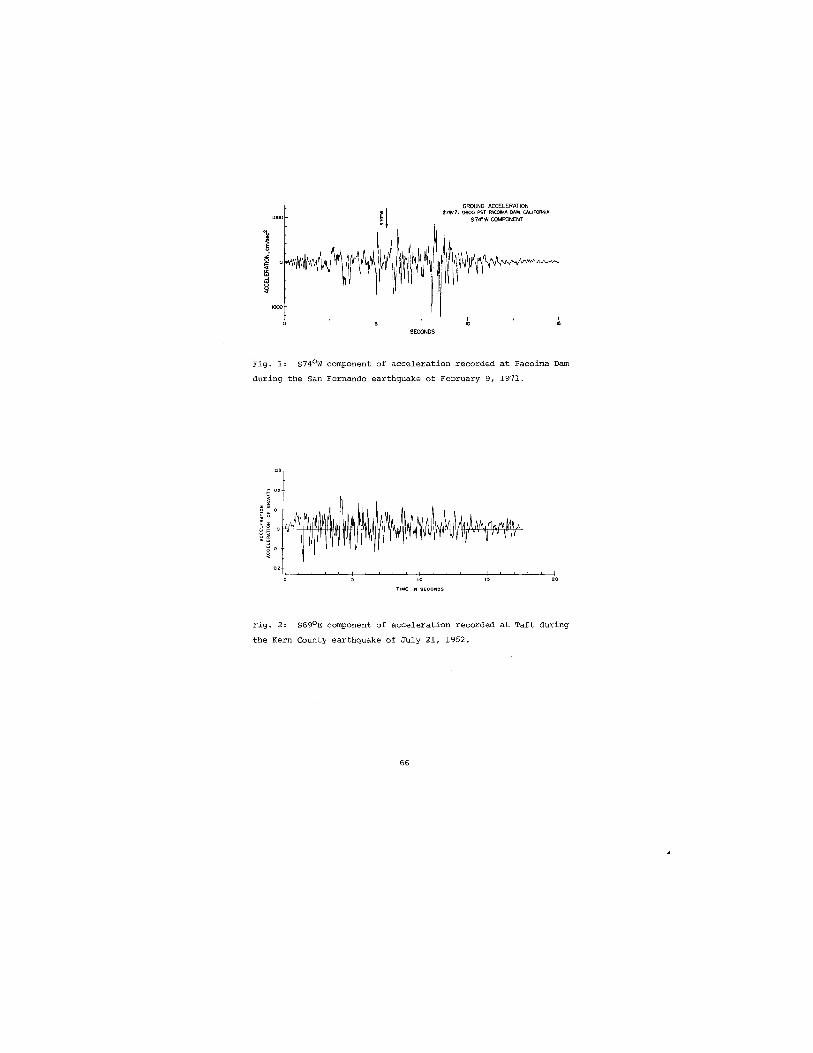
SECONDS

GROUND ACCELERATION 2/9111 0600 PST PACOIMA DAM, CALIFORNIA

S 74D W COMF'CNENT

1 10

1 ~

Fig. 1: S740W component of acceleration recorded at Pacoima Dam

during the San Fernando earthquake of February 9, 1971.

~·~--~~-L~~~-L~--~-,~~~--~~~--,~~~~~~~~io

TIME IN SECONOS

Fig. 2: S690 E component of acceleration recorded at Taft during

the Kern County earthquake of July 21, 1952.

66

Fig. 3: SMA-l Film-recording strong-motion

accelerograph.

Fig. 4: Strong-motion seismoscopes. Record is scribed on smoked glass

dish at top of instrument.

Another important strong-motion recorder is the seismoscope (S), illustrated in Figure 4.

This instrument is basically a spherical pendulum which scratches its displacement record

on a smoked watch glass, as seen in Figure 5. The natural period is commonly O~75 second

and the damping is nominally 10 percent of critical. The instrument and its properties are

such that the maximum displacement can be converted to a point on the displacement response

spectrum of the ground motion. Although it provides less information than the accelerograph,

the seismoscope has proven to be extremely reliable and in the Guatemalan earthquake of

1976, for example, provided the only significant strong-motion record. In addition to

direct reading of the instrument, there have been instances when it has been possible to

estimate the history of ground acceleration from the seismoscope response, using a higher

mode response of the transducer as a timing signal (12).

Fig. 5: Seismoscope record obtained at the University Admini­

stration building during the Guatemalan earthquake of February 4,

1976. North is to the left.

Other strong-motion instruments include such special purpose devices as peak-recording

accelerographs for nuclear powerplants, Carder "displacement" meters, elevator shut-off

mechanisms, and shut-off mechanisms (jiggle valves) for gas lines.

Status of Instrumental Networks

The principal agency involved in the deployment and maintenance of strong-motion instru­

ments, and in the processing of the records obtained, is the Seismic Engineering Branch of

the U. S. Geological Survey. This agency installs and maintains its own instruments and

performs similar services for instruments owned by other organizations. The operating

funds for the Seismic Engineering Branch are provided by the National Science Foundation

under a S-year agreement, scheduled to be renewed. Other sizeable networks are operated by

the California State Division of Mines and Geology, and by the City of Los Angeles. There

are additional, smaller networks operated by university research groups, utilities and other

organizations. Foreign accelerograph networks exist in several countries including Japan,

Mexico, Yugoslavia, Iran, Italy, New Zealand, peoples Republic of China, and Soviet Russia

among others.

As of June 1978 (9), the Seismic Engineering Branch is maintaining the following instru­

ments under its basic program:

184 USGS acce1erographs

59 accelerographs owned by other agencies

1 14-channe1 digital system

3 analog systems

20 accelerographs in foreign countries (chiefly

South and Central America), and

1 l2-channel analog system, in a foreign country.

An even larger number of accelerometers are owned by other agencies, (e.g., Corps of Engi­

neers, U. S. Bureau of Reclamation) but are maintained by the Seismic Engineering Branch

on a contract basis. This instrumentation includes:

301 acce1erographs

7 installations, with a total of 72 channels

of digitally-recorded data

4 installations, with a total of 38 channels

of analog-recorded data.

These figures give a total of 580 installations, with approximately 1864 channels of data.

The instruments are distributed thoughout the united States, with concentrations in more

seismic regions.

The Seismic Engineering Branch also owns and services approximately 150 seisrnoscopes

and maintains 25 peak recording accelerographs owned by other agencies. A few Carder dis­

placement meters are also owned and serviced by the Branch.

69

The program of the California Division of Mines and Geology was established in 1972 and

is operated by the Office of Strong-Motion Studies. The status of their installations,

as of June 30, 1978, is summarized below (13):

Installation Type Number Data Channels

Surface free-field 247 741

Down-hole free-field 18

Buildings 35 374

Dams 16 176

Bridges 3 ~ TOTALS 303 1,367

The free-field phase of the California program is approximately 50 percent completed

now, and emphasis in this phase has been shifted from general distribution throughout the

state toward the installation of special-purpose free-field instrumentation, including

linear and down-hole arrays.

The major· emphasis of the installation effort has recently been shifted to instrumenta­

tion of structures is about 10 percent complete.

The plans for the near future include instrumenting approximately 20 structures and

10 free-field sites per year, and the development of a capability for record processing

and dissemination.

The City of Los Angeles maintains a network of strong-motion instruments that have been

installed in tall buildings in accordance with the City Building Code. At the end of

August 1977 there were 158 buildings instrumented in this program, with a total of 486

three-channel accelerographs (11). The City of Los Angeles is maintaining 143 of these

buildings, while the others were maintained by other groups, including 10 serviced by

the Seismic Engineering Branch.

The remaining networks of strong-motion instruments are smaller and are generally de­

voted to special purposes of individual groups, such as the measurement of the response

of dams, the measurement of soil-structure interaction, or as complementary instrumenta­

tion for seismological research. An exception to this is the recently funded array being

installed by the University of Southern California. When completed this will comprise a

grid of about 90 accelerographs in the Los Angeles Basin.

The need for ~ncreased coverage by strong-motion instrumentation is recognized by all

seismically active countries, and there are plans underway for an international project to

install detailed arrays at selected locations in the world (7).

STRONG-MOTION DATA

Status of Strong-Motion Records

The Seismic Engineering Branch has the primary responsibility for processing, storing

and disseminating strong-motion records. They do this not only for the instruments they

70

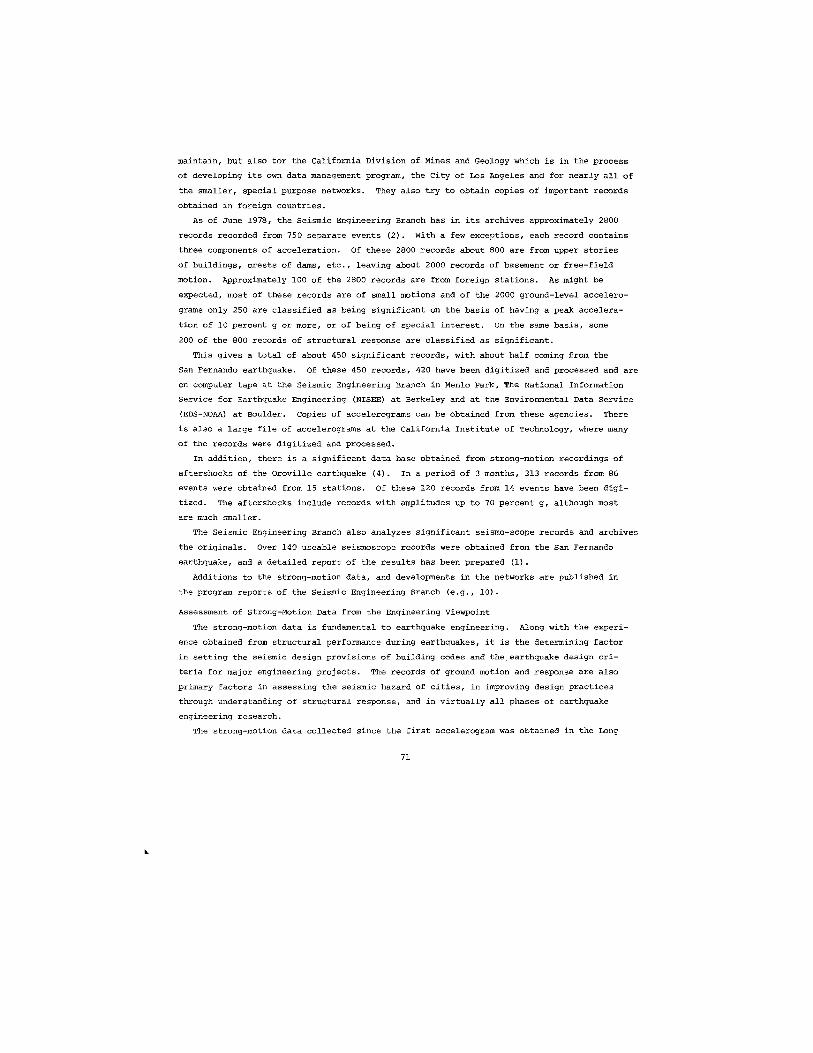
maintain, but also for the California Division of Mines and Geology which is in the process

of developing its own data management program, the City of Los Angeles and for nearly all of

the smaller, special purpose networks. They also try to obtain copies of important records

obtained in foreign countries.

As of June 1978, the Seismic Engineering Branch has in its archives approximately 2800

records recorded from 750 separate events (2). With a few exceptions, each record contains

three components of acceleration. Of these 2800 records about 800 are from upper stories

of buildings, crests of dams, etc., leaving about 2000 records of basement or free-field

motion. Approximately 100 of the 2800 records are from foreign stations. As might be

expected, most of these records are of small motions and of the 2000 ground-level accelero­

grams only 250 are classified as being significant on the basis of having a peak accelera­

tion of 10 percent g or more, or of being of special interest. On the same basis, some

200 of the 800 records of structural response are classified as significant.

This gives a total of about 450 significant records, with about half coming from the

San Fernando earthquake. Of these 450 records, 420 have been digitized and processed and are

on computer tape at the Seismic Engineering Branch in Menlo Park, The National Information

Service for Earthquake Engineering (NISEE) at Berkeley and at the Environmental Data Service

(EDS-NOAA) at Boulder. Copies of accelerograms can be obtained from these agencies. There

is also a large file of accelerograms at the California Institute of Technology, where many

of the records were digitized and processed.

In addition, there is a significant data base obtained from strong-motion recordings of

aftershocks of the Oroville earthquake (4). In a period of 3 months, 313 records from 86

events were obtained from 15 stations. Of these 120 records from 14 events have been digi­

tized. The aftershocks include records with amplitudes up to 70 percent g, although most

are much smaller.

The Seismic Engineering Branch also analyzes significant seismo-scope records and archives

the originals. Over 140 useable seismoscope records were obtained from the San Fernando

earthquake, and a detailed report of the results has been prepared (l).

Additions to the strong-motion data, and developments in the networks are published in

the program reports of the Seismic Engineering Branch (e.g., 10).

Assessment of strong-Motion Data from the Engineering Viewpoint

The strong-motion data is fundamental to earthquake engineering. Along with the experi­

ence obtained from structural performance during earthquakes, it is the determining factor

in setting the seismic design provisions of building codes and the. earthquake design cri­

teria for major engineering projects. The records of ground motion and response are also

primary factors in assessing the seismic hazard of cities, in improving design practices

through understanding of structural response, and in virtually all phases of earthquake

engineering research.

The strong-motion data collected since the first accelerogram was obtained in the Long

71

Beach earthquake of 1933 have greatly increased our understanding of the potential effects

of strong shaking and in general terms, our understanding is well-advanced. As engineers

and seismologists, we know something about the amplitude, frequency content and duration

of strong ground motion. We also have some appreciation of how these quantities are re­

lated to measures of the size of the earthquake and to the geometrical relations between

source and site. There are experimental data indicating the way th~t strong ground motion

can be affected by soil-structure interaction, by very soft soil deposits, by topography

and by the presence of surface waves. We are also in a position to make meaningful esti­

mates of some of the inherent variations that exist in strong ground shaking.

Although the general picture is encouraging, there are some very important questions

for which the data are insufficient. In addition, almost none of the points described

above are understood in sufficient detail, even given that complete understanding should

not be expected or required for applications in earthquake engineering practice. There

are two very important gaps in the data from the engineering viewpoint. First, there is

a paucity of records in the near field (e.g., ~ < 20 km) of major, potentially damaging

earthquakes. This lack of information introduces great difficulties, and occasionally

controversy, into setting the earthquake-resistant design criteria for major proJects.

The second major gap is the lack of strong motion records from a great (e.g., MS > 8)

earthquake. These earthquakes have, of course, the largest potential for disaster and

knowledge of the amplitude, duration and areal extent of strong shaking is required to deal

with the hazard posed by these extreme events. It should be pointed out also that there

are parallel gaps in our knowledge of the response of structures to ground motions in these

two categories.

There are major deficiencies in the data needed to clarify our understanding of the

effects of source mechanisms, travel paths and local conditions upop strong ground motion.

This is perhaps most apparent when relations between measures of the strength of ground

motion (e.g., peak acceleration, peak velocity, spectral intensity) and measures of dis­

tance (e.g., epicentral distance, hypocentral distance, distance to the center of the after­

shock zone) and earthquake size (e.g., local magnitude, MLI surface-wave magnitude, MS)

are investigated. Figures 6 and 7 are plots of peak acceleration and velocity, respec­

tively, for different magnitude classes. The figures illustrate the variability in the

data and suggest the difficulty in establishing simple relations among these variables.

The unsatisfactory state of present affairs is indicated by the fact that in a recent report

(6), 26 different studies were identified in which relations between peak acceleration,

magnitude and distance have been advanced. Clearly there is not yet a consensus on this

subject. An additional feature requiring experimental clarification and verification is

the effects of different source mechanisms on the strong motion. For example, theoretical

studies indicate, and some data support, the concept that thrust-type earthquakes produce

significantly stronger near field shaking than strike-slip events.

72

f­'-' 4 a: ':- 0.80 z o

~ a: w 0.60 -" w '-' ~ <i 0.40 f-Z o N

a: ~ 0.20

'" 4 W "-

o 00 A

• Magnitude 7-7.9

o Magnitude 6-6.9

Magnitude 5- 5.9

a Magnitude 4-4.9

°0~~~~'O~-L--02~0--~--3f,0~-L--~4~0--~~5~0~-L--~60~~--~7~0~-L---"80~~--~90 DISTANCE- km

Fig. 6: Peak acceleration vs. distance for four magnitude classes. Lines join the

two horizontal components of larger and closer motions.

73

120

100 u ., ~ E u • Magnitude 7-7,9 , >- 80. o Magnitude 6-6.9 I::: u .. Magnitude 5-5.9 0 o Magnitude 4-4.9 ...J W I >

60 i ...J <! r-z 0 N

0:: 40 0

I~ [1 I I

'" I g I 0

<! ! w

0:0 13io~4g "- 20 I ~ Ir 1 .. \ o ... " 0 0 f o 0 ...... o 0

00 10 20 30 40 50 60 70 80 90

DISTANCE -km

Fig. 7: Peak velocity vs. distance for four magnitude classes. Lines join the two

horizontal components of larger and closer motions.

Similarly, there is no clear professional consensus on the details of how local site

conditions can affect strong ground motion. Although there is general agreement on the quali­

tative nature of' such effects, there is a divergence of judgements on the degree of the

effects as seen in the data, the role of surface waves, and the degree to which engineering

solutions can be reliably obtained from analyses of simplified models of the phenomenon.

More strong-motion data clearly are required to further the understanding of the potential

effect of local conditions on the ground motions, and several of the strong-motion arrays

now being installed are designed to yield some of this data.

Additional strong-motion data are also needed to clarify the role of soil-structure

interaction in modifying the earthquake motion transmitted to the structure. The interaction

problems include the effects of the compliance of the foundation, the effects of embedment,

and the effects of foundations with large areas in suppressing motions of high frequency.

Some instrumental arrays now installed will provide records bearing on these problems, but

improvement is needed. For example, the effects of large foundations on high frequency mo­

tion appear to be quantitatively similar to effects soft soils are thought to have on these

motions. In the very common case of a record obtained in the base of a sizeable building

74

founded on fairly soft alluvium, it may not be possible to separate the two effects without

additional instrumentation.

Finally, it should be stated that the strong-motion data base is insufficient to deter­

mine the variability in strong ground motion under specified circumstances. The problem

arises, for example, when the level of the mean plus one standard deviation is sought for the

expected response spectra at a site of a nuclear power plant. Different investigations of

the existing data and different approaches to the assessment of the variability can lead to

significantly different results, with large economic implications for the project.

ACKNOWLEDGEMENT

The above discussion was taken with minor modification from the paper "Strong-Motion

Seismology" (8) which the author and Donald V. HeImberger prepared for presentation at the

second International Conference on Microzonation, held in San Francisco, November 26 -

December 1, 1978.

REFERENCES

1. Borrill, B. J., Seismoscope results -- San Fernando earthquake of 9 February 1971,

Chapter 3 of strong-Motion Instrumental Data on the San Fernando Earhtguake of February

9, 1971, D. E. Hudson (Ed.), Earthquake Engineering Research Laboratory, California

Institute of Technology, and Seismological Field Survey, National Oceanic and Atmospheric

Administration, U. S. Department of Commerce, Pasadena, California.

2. Brady, A. G., Personal communication, 1978.

3. Halverson, H., A technical review of recent strong motion accelerographs, Proceedings of

the Fifth Work Conference on Earthquake Engineering, I, 1046-1055, Edigraph, Rome, 1974.

4. Hanks, T. C. and L. C. seekins, Strong motion accelerograrns of the Oroville aftershocks

and peak acceleration data, Bull. Seism. Soc. Am., 68, No.3, 677-689, 1978.

5. Hudson, D. E. and W. K. Cloud, A simplified instrument ~or recording strong motion earth­

quakes, Bull. Seism. Soc. Am., ~, 159-174, 1961.

6. Idriss, I. M., State of the art -- ground motions, presented at the ASCE Earthquake Engi­

neering and Soil Dynamics Conference and Exhibit, Pasadena, California June 19-21, 1978.

7. Iwan, W. D. (Ed.), Proceedings of the International Workshop on Strong Motion Earthquake

Instrument Arrays, Honolulu, May 2-5. Earthquake Engineering Laboratory, California

Institute of Technology, 1978.

8. Jennings, P. C. and D. V. Helmberger,"Strong-Motion Seismology" presented at the second

International Conference of Microzonation, San Francisco, November 26 - December 1, 1978.

(To appear in the conference proceedings)

9. Maley, R. P., Personal communication, 1978.

10. Porcella, R. L. (Ed.), Seismic engineering program report, September - December 1977,

Geological Survey Circular 762-C, 1978.

11. Rabb, J. 0., Personal communication, 1978.

75

12. Scott, R. F., The calculation of horizontal accelerations from seismoscope records, Bull

Seism. Soc. Am., 63, No.5, 1637-1661, 1973.

13. Wooten, T.M.,Personal Communicat1on,

THE APPLICATION OF SYNTHETIC SEISMOGRAMS TO THE STUDY OF STRONG GROUND MOTION

Lane R. Johnson

University of California, Berkeley

Donald V. HeImberger

California Institute of Technology

The factors affecting strong ground motion during earthquakes can be divided into three

main areas: the source mechanism, wave propagation effects, and local site geology. In or­

der to interpret available strong motion data or make projections to strong motions that can

be expected during future earthquakes, it is important to understand how each of these factors

contributes to the strong motion. In this study, we have used a suite of synthetic seismo­

grams to arrive at some general conclusions concerning the effects that the source mechanism

and propagation have upon strong ground motion.

The basic dislocation model of an earthquake source (Burridge and Knopoff, 1964, Haskell,

1964, Haske22, 1969, Savage, 1966), is most commonly used for the purposes of modeling strong

ground motion. The effects of wave propagation are normally handled by calculating an appro­

priate Green's function and efficient methods for doing this are available (Ben-Menahem, 197~,

Helmberger, 1974, and Johnson, 1974). The combination of the source model and the Green's

function yields a synthetic record of the ground motion. Several studies have demonstrated

that reasonable assumptions about the mechanics of the source and the physical properties of

the crust lead to synthetic seismograms that closely approximate observed strong ground motion

records (Heaton and Heimberger, 1977, Heimberger and Johnson, 1977, Heimberger and Malone,

1975, Israel and Vered, 1977, Johnson and McEvilly, 1974, Savage, 1966).

Starting with the premise that synthetic seismograms have been used successfully to in­

terpret specific records of strong ground motion, the objective of this study was to deter­

mine what general conclusions about strong motion could be obtained from a systematic examin­

ation of synthetic seismograms. Synthetic seismograms were calculated in the epicentral range

of 4 to 128 km from a point dislocation source buried 8 km deep in a homogeneous elastic crust

32 km thick. In the sense that this is an oversimplified model for a realistic earthquake,

the results serve as a lower bound on the complexity to be expected in realistic ground motion.

At distances less than about four source depths, the synthetic strong motion records are

dominated by the direct P and S waves and the refracted sP wave. The near-field parts of the

elastodynamic solution are also prominent and affect primarily the interpretation of the long­

er periods of ground motion. At distances beyond about one crustal thickness, the effect of

the crust-mantle boundary becomes important and contributes to the complexity and duration of

ground motion.

Representative results are shown in Figure 1 which contains synthetic records of ground

displacement in the horizontal direction from a strike-slip type source. The transition from

a record dominated by body waves to one dominated by surface waves is clear. The large number

77

!::, (km) radial

32~

48~

64~

80~

96~

112~

128~ [

o 10 20 I ! " , ! ! !"!,, , I

T - !::,f6.2 (sec)

Fig. 1

~ c ID E ~ '" ~ " 0.1

, , , I I I I

001~1 --~~~~~~~~~~~~ 10 distance (km) 100

Fig. 2

of reflected and refracted waves with significant amplitudes is also noteworthy. For in­

stance, at a distance of 100 km, 26 different possible waves are predicted for the first 20

sec. of the record. The controlling criteria for the amplitudes of these waves are the radi­

ation pattern of the source and whether the distance is sufficient so that reflections take

place beyond critical angles.

Figure 2 summarizes the dependence of amplitude upon distance for the same type of source.

The maximum dynamic displacements are roughly constant for distances less than about one

source depth and exhibit a dependence that varies between (distan~e)-1/2 and (distance)-2 at

greater distances. The static displacements show a similar behavior except that the depend­

ence varies between (distance)-2 and (distance)-3 at large distances. At distances of about

one source depth the ratio between·the maximum dynamic and static displacements can be less

than 5.

78

REFERENCES

Ben-Menahem, A~ and M~ Vered, Extension and interpretation of the Cagniard-Pekeris method for

dislocation sources, Bull. Seise Soc. Am., 63, 1611-1636, 1973.

Burridge, R. and L. Knopoff, Body force equivalents for seismic dislocations, Bull. Seise Soc.

Am., 54, 1875-1888, 1964.

Haskell, N. A, Total energy and energy spectral density of elastic wave radiation from pro­

pagating faults, Bull. Seis. Soc. Am., 54, 1811-1841, 1964.

Heaton, T. H. and D. V. HeImberger, A study of the strong ground motion of the Borrego Moun­

tain, California, earthquake, Bull. Seise Soc. Am., 67, 315-330, 1977.

HeImberger, D. V" Generalized ray theory for shear dislocations, Bull. Seise Soc. Am., 64,

45-64, 1974.

HeImberger, D. V. and L. R. Johnson, Source parameters of moderate size earthquakes and the

importance of receiver crustal structure in interpreting observations of local earth­

quakes, Bull. Seis. Soc. Am., 67, 301-313, 1977.

HeImberger, D. V. and S. D. Malone, Modeling local earthquakes as shear dislocations in a

layered half-space, J. Geophys. Res., 80, 4881-4888, 1975.

Johnson, L. R., Green's function for Lamb's problem, Geophys. J. R. Astr. Soc., 37, 99-131,

1974.

Johnson, L. R. and T. V. MCEvilly, Near-field observations and source parameters of central

California earthquakes, Bull. Seis. Soc. Am., 64, 1855-1886, 1974.

Savage, J. C., Radiation from a realistic model of faulting, Bull. Seis. Soc. Am., 56, 577-

592, 1966.

Vered, M. and A. Ben-Menahem, Application of synthetic seismograms to the study of low-magni­

tude earthquakes and crustal structure in the northern Red Sea region, Bull. Seis. Soc.

Am., 64, 1221-1237, 1974.

79

SEMI-EMPIRICAL APPROACH TO PREDICTION OF

GROUND MOTIONS PRODUCED BY LARGE EARTHQUAKES

HiroD Kanarnori

California Institute of Technology

PROCEDURE FOR THE SYNTHESIS OF LONG-PERIOD GROUND MOTIONS PRODUCED BY GREAT EARTHQUAKES

We are primarily concerned with very long period (several seconds or longer) ground mo­

tion,generated by a great earthquake, expecially by a long transcurrent fault earthquake such

as the 1906 San Francisco or 1857 Fort Tejon earthquakes. Recent studies indicate that most

large earthquakes (e.g., Imamura, 1937; wyss and Brune, 1967; Trifunac and Brune, 1970) are

complex multiple events. For example, the 1976 Guatemalan earthquake (Kanamori and Stewart,

1978, see Figure 1) can be modeled by approximately 10 events with Ms ~ 6.5 (fault length 10

to 20 km) which occurred in sequence along the fault. Thus the ground motion from this type

of earthquake may be predicted by convolving the ground motion of the individual event with

the source function describing the space-time history of the multiple shock sequence. Re-

cent seismological studies have shown that for this period range, the ground disQlacement

caused by moderate size (fault-length ~ 20 km) earthquakes can be predicted by a Simple dis­

location model (e.g. Aki, 1968; Kanamori, 1972; Mikumo, 1973; Trifunac, 1974; Abe, 19749 ,b,1975

HeImberger and Malone, 1975; Burdick and Mellman, 1976; Langston, 1976; Langston and Butler,

1976; Heaton and HeImberger, 1977; Heaton and Helmberger, 1978). Since the individual event

of the Guatemala earthquake is probably small enough to be modeled by a simple dislocation

model, the above procedure may be useful for predicting long period ground motions produced

by a large earthquake.

A more empirical approach may also be used as follows. For the Guatemala earthquake, the

individual event is very similar to the 1968 Borrego Mountain earthquake, for which a detailed

source model has been determined (Burdick and Mellman, 1976; Heaton and HeImberger, 1977). A

recent analysis of strong motion and seismoscope records (Kartamori and Jennings, 1978; Jennings

and Kanamori, 1978) suggests that the Guatemala earthquake and the Borrego Mountain earthquake

have about the same ~ (local magnitude) indicating that the Borrego Mountain earthquake and

the individual event of the Guatemala earthquake are of about the same size at periods around

1 sec. This result suggests that long period ground motions produced by a Guatemala type

earthquake may be empirically predicted by convolving the appropriately scaled ground motion

produced by the Borrego Mountain earthquake with the source time sequence of the Guatemala

earthquake.

ESTIMATION OF THE MAXIMUM AMPLITUDE OF STRONG MOTION FROM THE LOCAL MAGNITUDE ~

Despite the recent progress in seismology, it is still very difficult to predict short­

period (eg., less that 2 sec.) ground motion by using existing methods. One possible approach

to this problem is to use the local magnitude, ML

. The local magnitude, ML

, has direct re1e-

80

Multiple Event

;10 Source time function

Analysis

----36~ 1-1-=9-1

seC-A ~ 1: ~ s(t)

-/'-+ V + '-V'--P pP sP sum

[Sit) - ~ m, 5(1-1; )]2_ minimum 1=1

COP (6=8397)

~ /---j

1 min

I 1.6 X 1026

dyne-em

KEV (6=84.5°)

~fVlAM!\~

~ 1,111111 12.5,1026

I KJF (6=87.5°)

~MI\ MA h...,A

~ I, II III I 12.2,1026

I

~ ull~I"I~I~II~1 ~I ___ 11.6,1026

dyne-em

I 1.8 xl026

dyne-em

KTG (6=68.2°)

~f'\r'\ JI!\ I'I.AMf.,

~ II I I I I III 12.1,1026

STU (6=84.2°)

~ ,,-1\\ Ivotl\ A."

~ I, I, till I I 3.0,10 26

Fig~ 1: Observed and synthetic P waves for individual WWSSN stations obtained

from the multiple shock analysis. For each station the source time series is

obtained using the source time function shown here. The surface reflections pP

and sP are included in the source time function. The resulting series is given

for each station along with the moment for the first event. The height of the

vertical bar is proportional to the moment of the individual event. 8 is the

epicentral distance.

81

vance to engineering applications because ~ is determined within the period range of great­

est engineering interest (0.3 to 2 sec.). However, ML has been traditionally determined by

using high gain seismographs (e.g., the Wood-Anderson seismograph). Hence, most of the re­

cords of very large earthquakes go off scale at short distances precluding their use in deter­

mining MLo For large earthquakes (ML ~ 5.5), ML is determined only at large distances. Since

correction for the decay of the amplitude as a function of distance is incorporated in the

ML scale, the values of ML should not depend upon the distance. However, the amplitude-dis­

tance curve used in the ML scale is calibrated by using small earthquakes so that it is not

clear whether it also applies to very large earthquakes.

It is possible that, for very large earthquakes, complex interference of seismic waves

originating from different parts of the fault plane may significantly affect the decay rate

of the maximum amplitude resulting in distance dependent ~.

Recently, Kanamori and Jennings (1978) showed that strong motion accelerograms can be

used to calculate a synthetic Wood-Anderson response by which ML can be determined at short

distances (see Figure 2)0

~ 1.5 8 "-' ~ 1.0 C> 0-

~ '" ~ '" "-' ~ <:

= C> C> ~ 1.0 X

10 20 30 40 50 60 TIME (SEC)

Fig. 2: Comparison of the record observed by a 4X torsion seismograph (upper trace)

with the 4X wood-Anderson response calculated from the strong-motion record. The re­

cords are the N-S component of the 1971 San Fernando earthquake obtained at the Seis­

mological Laboratory at the California Institute of Technology.

82

Figure 3 shows the value of ~ as a function of distance for several California earthquakes.

All the data points are obtained from ML determined from strong-motion accelerograms. Al­

though data are not complete, there is no obvious dependence of ML on distance suggesting

that the amplitude decay curve currently used is applicable to these large earthquakes. If

this is the case, the value of ML = 7.2 for the Kern County earthquake would predict a maxi­

mum amplitude on Wood-Anderson records of 440 rn at a distance of 10 kID from the epicenter

which suggests an amplitude, velocity, and acceleration of ground motion of 25 em, 2 m/sec.,

and 1.58 g respectively, if a predominant period of 0.8 sec. is assumed (see Figure 4). Be­

cause of the lack of close-in strong motion data from very large earthquakes, the above re­

sult should be considered tentative. However, this approach, when more close-in data are

obtained, will provide a useful estimate of the maximum ground motion on the basis of seis­

mological consideration.

SOY? urnondo, 197/ 7

o fDa 200

8 Kern (ounl!!, /952

7 oL------------Jo~0-----------2~0~0------

Ll, km

BorreJo fff.) /9G8

7 >40$S14S%S6>SSSXik

6'------...L.-------::-':-:----o faa 200

Lljfle Crul<, /970

50L---------~f~0~O--------~2~0~O~--­

Ll, km

Fig. 3: ~ as a function of distance

for several California earthquakes. The

hatched zone indicates the mean + one

standard deviation.

Fig. 4: The maximum displacement A, velocity V, and

acceleration a. at a distance of 10 krn as a function

M The L

solid lines are for a period of 0.8 sec.

and the dashed lines are for a period of 0.3 sec.

83

REFEREMCES

Abe, K~, Seismic displacement and ground motion near a fault: The Saitama earthquake of

September 21, 1931, J. Geophys. Res., ~, 4393-4399, 1974a.

Abe, K., Fault parameters determined by near- and far-field data: The Wakasa bay earthquake

of March 26, 1963, Bull. seis. Soc. Am., 64, 1369-1382, 1974b.

Abe, K. f Static and dynamic parameters of the Saitama earthquake of July 1, 1968, Tectonophy

sics, in press, 1975a.

Aki, K., Seismic displacement near a fault, J. Geophys. Res., Il, 5359-5376, 1968.

Burdick, L. ~., and G. R. Mellman, Inversion of the body waves from the Borrego Mountain

earthquake to the source mechanism, Bull. Sesi. Soc. Am., 66,'1485-1499, 1976.

Heaton, T. H., and D. V. HeImberger, A study of the strong ground motion of the Borrego

Mountain, California earthquake, Bull. Seise Soc. Am., 67, 315-330, 1977.

Heaton, T. H., and D. V. HeImberger, Predictability of strong ground motion in the Imperial

Valley, Bull. seis. Soc. Am., in press, 1978.

HeImberger, D. V., and S. D. Malone, Modeling local earthquakes as shear dislocations in a

layered half space, J. Geophys. Res., 80, 4881-4888, 1975.

Imamura, A., Theoretical and Applied Seismology, Maruzek, Tokyo, 358, 1937.

Jennings, P. C., and H. Kanamori, Determination of local magnitude, ML

, from seismoscope re­

cords, in preparation to be submitted to Bull. Seis. Soc. Am., 1978.

Kanamori, H., Determination of effective tectonic stress associated with earthquake faulting­

Tottori earthquake of 1943, Phys. Earth Planet. Interiors, 2' 426-434, 1972.

Kanamori, H., and G. S. Stewart, Seismological aspects of the Guatemala earthquake of Feb.

4, 1976, J. Geophys. Res., in press, 1978.

Kanamori, H., and P. C. Jennings, Determination of local magnitude, ML

, from strong motion

accelerograms, Bull. Seise Soc. Am., in press, 1978.

Langston, C. A., A body wave inversion of the Koyna, India earthquake of December 10, 1967,

and some implications for body wave focal mechanisms, J. Geophys. Res., 81, 2517-2529,

1976.

Langston, C. A., and R. Butler, Focal mechanism of the August 1, 1975, Oroville earthquake,

Bull. Seis. Soc. Am., 66, 1111-1120, 1976.

Mikumo, T., Faulting process of the San Fernando earthquake of February 9, 1971 inferred

from static and dynamic near-field displacements, Bull. Seis. Soc. Am., 63, 249-269,

1973.

Trifunac, M. D., A three-dimensional dislocation model for the San Fernando, California

earthquake of February 9, 1971, Bull. Seis. Soc. Am., 64, 149-172, 1974.

Trifunac, M. D., and J. N. Brune, Complexity of energy release during the Imperial Valley,

California, earthquake of 1940, Bull. Seis. soc. Am., 60, 137-160, 1970.

Wyss, M., and J. Brune, The Alaska earthquake of 28 March 1964: A complex multiple rupture,

Bull. Seis. Soc. Am., 22, 1017-1023, 1967.

84

DETERMINISTIC MODELING OF SOURCE MECHANISMS UTILIZING

NEAR- AND FAR-FIELD SEISMIC DATA, THE 1971

SAN FERNANDO EARTHQUAKE

Charles A. Langston

Pennsylvania state University

Depending on frequency band, instrument characteristics, distance from source, and

other factors, seismic radiation from earthquakes is categorized in many ways by both geo­

physicists and engineers. As a result of this data division, inversions for source processes

and geometry through application of deterministic models often do not utilize the possible

constraints which may occur in other data categories. Rather, many studies are very restric­

tive and apply a particular model or modeling technique to a limited data subset, thereby

increasing uniqueness problems. Recognizing that non uniqueness is the greatest problem

in all geophysical studies, it therefore seems reasonable to adopt a more global modeling

concept in which the earthquake and its physical processes assume the central focus. Models

for the earthquake must satisfy all observed data or must otherwise be discarded. An effi­

cient way to arrive at a model or set of models is to examine as much of the data as possible

to determine a set of constraints.

With this philosophy in mind, teleseismic P, SV, and SH waves recorded by the WWSS and

Canadian networks from the 1971 San Fernando earthquake were modeled in the time domain to

determine detailed features of the source as a prelude to studying the near and local field

strong motion observations. Synthetic seismograms were computed from the model of a propa­

gating finite dislocation line source imbedded in layered elastic media. The effects of

source geometry and directivity were found to be important features of the long period ob­

servation. The most dramatic feature of the model was the requirement that the fault, which

initially ruptured at a depth of 13 km as determined from pP-P times, continuously propagated

towards the free surface, first on a plane dipping 530

NE, then broke over to a 290

NE dippi.ng

fault segment. This effect is cle:arly shown in the azimuthal variation of both long period

P and SH waveforms. Figure 1 shows observed (top) and synthetic (bottom) P waveforms at 17

wwss and Canadian network stations for the final inferred fault model. The P first motion

plot is represented by the equal area projection of the lower half of the focal sphere. The

nodal planes are for the bottom (solid lines) and top (dashed lines) sections of the final

fault model. Note the prominent dilatational arrival approximately 10 seconds into the P

waveforms for stations in the northern and western azimuths. This arrival, which disappears

for stations in eastern and southern azimuths, is interpreted to be the combined effect of P,

pP, and sP from the top section of the San Fernando Fault.

Figure 2 demonstrates the good sensitivity that the long period data have for some of

the model parameters. Comparisons of theoretical waveforms with representative observed P,

85

26 MO (xiO • dyne cm) San Fernando Vertical N01lvY-1.38 T~R' OA8 .p Wlveforms

1 Nadal Planes 01 02

8 53° 29°

M8~"91 FS,#-'AO P~"0'94' ~-i~:-~ Obs. Syn.

=~ ~-~" _oc~ '\ see GE~O'88

HNR

\ GEO

::"'~:::::HSJG NAT

_/ CAR a, LPS

QUI ~ __ -'lLPB

I---50 sec-----l

Fig. 1

1--50 seC------i

Fig. 2

86

Surface &€<lk

ssw'6 t 14

Fault Geometry used

in Model calculations

• Compression P

° Dilatation P

Son GotJ'oeI Foull,Zore

6 4

A

o

8 I

- 10

Fig. 3

-2 NNE

SV, and SH waveforms are shown. The first letter of eac~ model represents the fault geometry

shown in Figure 3. Geometry U is unilateral rupture from the hypocenter to the free-surface

on the 530 dipping plane. A, B, and C designate fault plane breakover points at 9, 5, and 3

km depths, respectively. The values and 2 after each letter indicate rupture velocity in

km/sec. RUpture starts at 13 km depth and propagates up the fault. Figure 2 demonstrates

that wave duration and relative peak timing are closely related to rupture velocity. Relative

amplitudes in each waveform indicate orientation. From similar model comparisons with all the

data, the average rupture velocity from hypocenter to surface is constrained to be, at most,

1. 8 km/sec.

Results from analysis of teleseismic short period P waves suggest further constraints on

the nature of the initial rupture. Although attenuation and interference with radiation from

the fault are possible, complications, comparison of long and short period P, and short period

pP and P waves suggest that rupture was initially bilateral, or possibly, strongly unilateral

downwards, propagating to about 15 km depth. Figure 4 condenses the results of many modeling

experiments performed to e~plain the anomalously large short period P to pP amplitude ratio.

For the orientation determined from a well constrained long period fault plane solution, pP

should be as large or larger in amplitude as P for a point source or unilaterally upward pro-

0.5 \::Uniloterol up VR~1.8

00 40 eo 120 (6) 200 240 280 320 360 AZimuth. deg

Fig. 4

pagating rupture. Points shown in Figure 4 are P-pP amplitude ratios taken from a stacking

procedure and corrected for radiation pattern and the free-surface reflection coefficient.

Lines are expected amplitude ratios for models in which the rup~ure velocity was allowed to

differ for updip and downdip directions around the hypocenter. The best agreement occurs

for those models in which rupture is faster downward. Long period P-short period P wave am­

plitudes do not discriminate between these models well, except for ruling out the simple uni­

laterally upward propagation.

87

These geometrical and dynamical constraints determined from teleseismic wave shape and am­

plitude data are not totally met by any previous model determined from dynamic near-field

data. The complication of initial faulting occurring bilaterally or unilaterally downwards

qualitatively affects understanding of the initiation of faulting and state of stress in hypo­

central region. Of course, these simple models for the teleseismic data must be further modi­

fied as other constraints are determined from near-field dynamical models and other data in

an iterative procedure. It is hoped that future studies of source processes and mechanisms

will incorporate more diverse sources of data with greater effort to reduce uniqueness pro­

blems.

SELECTED REFERENCES

Langston, C. A., and D. V. HeImberger, A Procedure for Modeling Shallow Dislocation Sources,

Geophys. J. R. astr. Soc. 42, 117-130, 1975.

Langston, C. A., The February 9, 1971 San Fernando Earthquake: A Study of Source Finiteness

in Teleseismic Body Waves, Bull. Seis. Soc. Am. 68, 1978.

88

OCCURRENCE OF STRONG GROUND MOTIONS

R. B. Matthiesen

USGS, Menlo Park, CA

The availability of data from several stations at which strong motion accelerographs

have been installed for about 40 years provides for a direct evaluation of the "recurrence"

of strong ground motions at those sites. The records obtained fram the site at Hollister,

which was installed in 1944, are used for illustration. In Figure 1 the cumulative number of

events for which peak accelerations exceeded four selected values are plotted vs the year in

which the event occurred. Similar results can be obtained for each value of peak acceleration

recorded at the site. The slopes of the IIbest fitll straight lines define the "events per

year" for each value of peak acceleration, whereas the deviations from the straight lines in­

dicate the extent to which the concept of "recurrence" is not applicable. No attempt has

been made to distinguish between foreshocks, rnainshocks, and aftershocks in compiling these

data, so that clustering of the data may be an indication of foreshock or afterschock activity

associated with a mainshock. Obviously, the inclusion of such data influences the interpre­

tation of the final results.

30~----------------------~

HOLLISTER

20

10

1960 YEAR

Fig. 1

1970

HOLLISTER

O.OIILO-L...I.....L..l.L..l.lJ"I!=r,O--'-.....L...J..J...~I~

ACCELERATION - em/sec"

Fig. 2

The "events per year" as obtained from the slopes of the IIbest fitll lines can be plotted

vs each successive value of recorded peak acceleration to obtain a IIrecurrence" curve as

shown in Figure 2. Thus, the four sets of data shown in Figure I, which were selected for

illustration, represent only four of the data points shown in Figure 2. The slope of the

"recurrence" line indicates a lib" value of about -1.0, which is in agreement with values ob­

tained from regional recurrence studies ( see Algermissen and Perkins, 1976, for example).

Similar studies were made for 21 other sites. In seven cases, the recurrence curves indicate

89

D

"bl! values of about -1.0, but only in three cases is there sufficient data to place some con­

fidence in the results. Furthermore, it is significant that for 14 sites at which strong mo­

tion accelerographs have been installed for more than forty years, the amount of data is not

sufficient to define recurrence curves.

In order to extend this study of recurrence of strong ground motions to other sites, the

occurrence of MMIT = VI or greater events have been evaluated for selected sites in regions of

relatively high activity. The data set used in the evaluation was the compilation by Coffman

and von Hake (1973). This is believed to be a reasonably consistent set for most of the

country for the period from 1870 to 1970, although no such compilation can be expected to be

uniformly consistent, complete, or totally accurate. Only events of MMI = VI or greater have

been considered since lower intensities are associated with ground motions below the thres­

hold of significant strong ground motion (say, a maximum ground acceleration of 0.05 g). For

each event was approximated as a circle drawn around the epicenter, as illustrated in Figure 3.

On these maps the areas in which several strong-motion records could have been obtained are

indicated by the overlapping of the circles, and the number of events that would have caused

significant ground motions at a particular site can be determined by counting the number of

ti~es that the site is encircled by the MMI = VI contours.

CUMMULATIVE NUMBER OF EVENTS

18700 i5 ;:; !'l

1880 ~ ~

1890 1i ~ ~

"' 0 ::> I-

~ -<

~ \ 1930

\ 1940

1950

1980

1970 LONGITUDE - degrees

Fig. ~ Fig. 4

By identifying the events associated with the MMI = VI contours encircling a site, a

history of possible strong-motion recording at any specific site may be projected, and the

cumulative number of events vs the date of projected recording may be plotted. If the con­

cept of "recurrence" has meaning, such projected histories should indicate a linear relation

between the number of events and the date of Occurrence. The projected history at Hollister

9Q

is shown in Figure 4. This is in agreement with the actual history of strong motion record­

ing at the site since 1940, but indicates a quiescent period from 1906 to 1940. Hollister is

near the southern end of the 1906 fault rupture. This suggests that the state of stress in

the Hollister area was relieved by the 1906 event and that the present rate of 4 years per

event is "back to normal".

This brief study of the occurrence of strong ground motions indicates that the concept

of "recurrence" applies in a limited sense to many sites, but when looked at with a jaundiced

eye the conclusions are the same as those stated by McGuire (1977): " ••. the most recent past

is the best indicator of seismic activity in the near future, ••• ", but " •.• a large amount of

data cannot be indiscrinirnately thrown together to calculate a mean activity rate .. "

REFERENCES

Algerrnissen, S. T. and D. M. Perkins, A Probabilistic Estimate of Maximum Acceleration in

Rock in the Contiguous United States, USGS, Open File Report 76-416, 1976.

Coffman, J. L. and C. A. von Hake, Earthquake History of the United States, NOAA, Publication

41-1, 1973.

McGuire, Robin K., Insights from the Chinese Catalog of Stationary Models Used for Seismic

Hazard Assessment, USGS, Open File Report 77-715.

91

THE NEEDS OF THE NUCLEAR REGULATORY COMMISSION IN THE

FIELD OF STRONG MOTION SEISMOLOGY

LEON REITER

u.s. Nuclear Regulatory Commission

The Nuclear Regulatory Commission (NRC) looks to the seismological and engineering

community to help develop methods that provide reliable estimates of earthquake induced

ground motion at different levels of risk for various sites throughout the country_ These

estimates should be in a form permitting effective use by geotechnical and structural engi­

neers in the evaluation of sites and the design of structures for nuclear related facilities.

Our needs generally parallel other engineering needs except that most nuclear facilities

must be designed to be safe at very low levels of acceptable risk. Much recent research in

strong motion seismology has been related directly or indirectly to nuclear power plant de­

sign so that our needs and problems have had an impact upon the trends within the science

as a whole.

The problems we see today and the questions that we believe need answering can be

divided into areas related to the earthquake source, seismic wave type and propagation, site

effects, and engineering input.

EARTHQUAKE SOURCE

The most difficult problem we face today is estimating strong motion in the vicinity

of the earthquake source, i.e., the near-field. No nuclear power plant is intentionally

placed near a known earthquake source or "capable" fault but subsequent investigations have

revealed new faults and resulted in reass~ssment of some old faults. The Humboldt Bay,

Diablo Canyon, San Onofre, and Vallecitos sites in California are the prime examples. In

order to determine whether facilities at these sites are sufficiently safe as designed, need

to be upgraded or need to be abandoned, requires an assessment of motion near earthquake

sources where we have few measurements most of which are from small earthquakes. One approach

has been to extrapolate inward from records taken at longer epicentral distances. How valid

can this approach be when the particular physical and geometric configuration of the source,

which apparently is dominant in controlling the near-field motion, is of secondary importance

in the far-field. Are the more elegant theoretical models and numerical procedures for cal­

culating the motion from these models in a stage where their results can be considered re­

liable?

Other aspects of the earthquake source problem relate to the eastern u.S. It has been

postulated that intraplate earthquakes hav~ higher stress drops than interplate earthquakes.

If so can we expect and should we design for the increased amplitudes at the high frequencies

believed to be associated with increased stress drops? While earthquakes in the East cannot

be associated with surface faulting and the larger events appear to be occurring at hypo-

central depths of at least 10 kilometers, there are several occurrences of small near sur­

face events that have resulted in very small felt areas of relatively high intensity. The

magnitude 3.8, Intensity VII, event of August 14, 1965 in Cairo, Illinois is one such ex­

ample. It is believed to have had a focal depth of approximately 1 km. These events l.ave

not been associated with structure. What magnitude may these events reach and what charac­

terizes their ground motion?

WAVE TYPE AND PROPAGATION

Most present techniques such as those used to estimate soil response utiljze models

of ground motion which assume a predominance of vertically propagating, horizontally polar­

ized shear waves. Studies of records such as those from the San Fernando earthquake show

the importance of other types of waves, particularly surface waves. We must obtain better

quantitative estimates of the different wave types involved in strong ground motion and

the impact these will have upon structural design. To what extent does the existence of

horizontally propagating waves result in the reduced effectiveness of an earthquake upon

structures with large foundations? To what extent does the existence of these waves also

result in rocking or torsional motions not previously considered?

A regional propagation difference is apparent between the eastern and western u.S.

The much larger felt areas for similar sized earthquakes in the East necessitates consider­

ation of the effect of distant (greater than 100 km) large events such as New Madrid. In

what ways is damaging ground motion from these earthquakes different than that from sources

less than 100 km away? Is increasing the long period part of the design response spectrum

enough to account for the lower attenuation? If so, how much?

SITE DEPENDENCE

The most frequent problem we face is that of how to incorporate differences in site

geology into estimates of free-field ground motions. Several investigators have classi­

fied sites in three or four broad categories and have shown differences in ground motion

parameters such as peak acceleration and spectral shape associated with each category. The

variation within each category however is rather large and it is not clear how significant

the differences are. Investigations NRC has funded indicate that the surficial classifi­

cation of accelerometer site conditions often is not confirmed by borings made in field

investigations. All the comparative studies show relatively higher acceleration at rock

for periods less than 0.5 sec. Since most safety related structures at nuclear power plants

have periods equal to or less than 0.5 sec., does this mean it is less safe to build on rock

than on soft sites? Observations of earthquake damage do not sup~ort this conclusion. Given

the existing data base and state of our knowledge with respect to strong motion recording

sites, how detailed a categorization is possible?

Along with differences in site properties the effects of depth upon ground motion are

also of great importance. Present techniques of deconvolution need to be more uniformly

specified as to what ground motion is used and where the input is assumed. Are the present

computational techniques adequate in providing estimates within a wide enough period range?

Some individuals utilizing these techniques complain of irrational results which they attri­

bute to the computational techniques. What are the limiting conditions to which deconvolu­

tion may be presently applied? Ground motion at depth is not only a problem with respect to

foundations several tens of feet below the surface but is also of critical importance in the

design of waste repositories at depths of hundreds or even thousands of feet.

ENGINEERING INPUT

Most present methods utilize standard response spectral shapes whose absolute level

is determined by peak acceleration. The relatively high peak accelerations associated with

some damaging earthquakes raises serious questions as to the validity of this approximation.

Should we use other peak parameters such as velocity and displacement? Should we as some of

us have suggested use a lower lIeffective ll acceleration? If so how may this parameter be re­

liably estimated? Should we abandon reference values completely and go directly to each

spectral ordinate given source and site characteristics? All the above questions assume that

the response spectrum and related time history are seismological inputs that adequately de­

scribe ground motion far engineering purposes. Long durations however are not adequately re­

flected in the response spectra required by the NRC and are believed to be a critical factor

in determining damage from large earthquakes. HOw, and to what extent, should duration of

strong motion be incorporated into seismological input? Does it require a change in instru­

mentation so as to make a more faithful recovery of ground displacement? What is the dura­tion to be considered in liquefaction studies?

Finally, any designed structures including those relate~ to nuclear facilities entail

the acceptance of some risk. Very often the most minimal of risks have to be weighed against

other societal factors. Estimating these risks is a difficult and complex problem. The

ability to place expected earthquake ground motion into a quantitative probabilistic frame­

work would be an important contribution to arriving at both reasonable and reliable estimates

of this risk.

SOME THOUGHTS ON THE DEFINITION OF THE INPUT E~RTHQUAKE

FOR THE SEISMIC ANALYSIS OF STRUCTURES

Jose M. Roesset Massachusetts Institute of Technology

It has become customary in the seismic analysis of special structures, such as nuclear

power plants, to define the input earthquake by a maximum ground acceleration (resulting from

a seismic risk study with varying degrees of sophistication) and a family of smoothed univer­

sal response spectra. These spectra represent an envelope of the results for a collection of

real earthquakes with different characteristics. One or more artificial earthquakes are then

generated so as to match (more or less closely) the specified spectra, sealed to the desired

peak ground acceleration. The motions are assumed to occur at the free-surface of the soil

in the free-field (without disturbance .by the structure).

This procedure is based on a series of simplifications which may be justified for an

approximate design, but which appear inconsistent with the degree of refinement sought in the

other phases of the analysis. The inconsistencies become more striking and may lead to un­

realistic results when more complex met~odologies, such as the use of probabilistic formula­

tions or nonlinear dynamic analyses, are implemented. Efforts to improve this situation have

not been, however, very successful in the past.

It would appear that more logical alternatives would be possible if we had the ability

to construct realistic earthquake motions as a function of source mechanism, magnitude, epi­

central distance, and overall geological and local soil conditions. One could then, in the

seismic risk analysis, consider separately the various possible sources and derive for each

one a probable motion, instead of lumping them together under the assumption of similar char­

acteristics.

The specification of the design earthquake at the free-surface of the soil within the

present procedure is reasonable when the soil can be classified as firm ground or with sim­

ilar general characteristics as the sites at which the various records used to construct the

envelope spectra were obtained. The use of these spectra for rock or for a very soft soil

deposit would be, however r unrealistic.

Given the motion at the surface, it is normally necessary to make some assumptions as to

the kind of waves that constitute the earthquake. For an embedded foundation, if the sub­

structure method or three-step approach is used, it is first necessary to determine compat­

ible motions (including rotations) at the foundation level, considering a massless foundation

(this is the so-called kinematic interaction or wave scattering problem). But even if the

foundation is at the surface and the input motion is applied directly at the base (including

the soil compliances to account for soil structure interaction effects), one is in fact assum­

ing implicitly that the horizontal motions are due to shear waves propagating vertically and

the vertical motions are caused by vertically polarized P waves. When using the direct

95

SIMULATIONS OF EARTHQUAKE GROUND MOTIONS

Ralph A. Wiggins, Gerald A. Frazier,

Joel Sweet, and Randy J. Apsel

Delta Associates

A study has been undertaken to find a simple computer model that will simulate strong

motion records near strike-slip earthquakes. The ultimate application for these simulations

is for engineering design of structures. Hence, the study has been focused primarily on

modeling response spectra at frequencies from 1. to 20. hz. The computer model has been

tested by predicting response spectra for the 1940 Imperial Valley, 1966 Parkfield, and 1976

Brawley ftarthquakes.

The computer model that has been developed for simulating earthquakes is partitioned

into three basic steps as described below.

FRACTURE SIMULATION

A three dimensional finite element code (SWIS) was used in. conjunction with analytical

solutions and laboratory experiments to provide information on how fault slip occurs during

an earthquake (Archuleta and Frazier, 1978). Experiments performed on compressed rock

specimens indicate that shear fracture occurs when the shear stress exceeds some limiting

value in the neighborhood of one kbar. (The actual failure strength depends on rock composi­

tion, loading rate, the presence of cracks, confining pressure, and interspersed fluid.) The

fracture strength of rocks can then be related to the maximum velocity of particles on the

fault surface near the crack tip.

The physics ·of spontaneous shear fracture is contained in our characterization of fault

slip. The following parameters are pertinent:

(a) Rupture Velocity: The rupture initiates at a point on the fault surface

and spreads at a velocity which is taken as a fraction of the local shear

wave velocity. sensitivity studies have been performed with rupture velocity

varying from 50% to 90% of the shear wave velocity, the upper limit being set

at the Rayleigh wave velocity according to fracture mechanics.

(b) Dynamic Stress Drop: Large particle accelerations occUr at points on the

fault where new crack surface is being produced due to concentrations in

stress. Immediately following the production of new crack surface, the

shear stress drops to a lower value almost instantaneously. This effect is

characterized in the slip function by a peak in the slip velocity at rupture

initiation. This rapid slip, which can be related to dynamic stress drop

using simplified mechanics, occurs for a brief interval of time while the

crack extends a few tens of meters.

98

(c) Static Stress Drop: The static stress drop is a measure of the average

difference in shear stress before and after an earthquake. The average

final offset on the fault is linearly related to the static stress drop

when the rupture area is held constant. After the initial peak, the

slip velocity drops to a uniform value consistent with the static stress

drop and rise time.

(d) Rise Time: Rise time is a measure of the duration of fault slip at a

single point. SWIS calculations indicate that the rise time is controlled

by the time it takes for information from non sliding portions on the fault

surface to propagate to points where sliding is occurring. On the average,

the rise time appears to be the time it takes for the shear wave velocity

to traverse the fault width.

(e) Spatial Variations: In an actual earthquake, slip characteristics inevitably

vary in some complex manner over the fault surface. In an effort to minimize

the number of earthquake parameters the same slip function is used for all

points on the rupture surface.

WAVE PROPAGATION

An analytical code (PROSE) has been developed to propagate seismic waves in horizontally

layered, viscoelastic earth. The method accurately synthesizes the multiplicity of waves

that arise in a horizontally layered medium over the frequency range from 0.1 to 20. Hz.

Green1s functions are obtained using the appropriate geologic layering for wave contributions

that result from rapid slip over small fault segments which are distributed over the surface

of impending rupture. Several hundred of these Green's functions are obtained for a single

earthquake to insure accurate simuiation of the seismic energy that radiates from all por­

tions of the rupture surface.

The earth's crustal structure is characterized by horizontal, viscoelastic layers to a

depth in excess of 20 km. Each layer is defined by the parameters: layer thickness, dens­

ity, shear wave velocity, compressional wave velocity, and quality factor (Q). The quality

factor for each layer is empirically related to the shear-wave velocity using both seismic

evidence and laboratory data for guidelines. For cases in which conflicting evidence occurs,

we have chosen to rely on that evidence with the largest quality factor, i.e., we use the

smallest material attenuation that is consistent with the available data.

GROUND MOTION

The fault slip, based on calculations by SWIS, is combined with the wave propagation

produced by PROSE to produce synthetiC earthquake motions using a convolution code (FALTUNG).

The prescription of fault slip is convolved both in time and space over the rupture surface,

with the elementary solutions from PROSE to produce synthetic ground motion at selected

99

points on the earth's surface over the frequency range from 0.1 to 20. Hz.

VALIDATION STUDIES

The range of validity of the computer mOdel has been tested by simulating three past

earthquakes Brawley (1976), Imperial Valley (1940), and Parkfield (1966). For all three

earthquakes best fits are obtained for a rupture velocity of 90% of the shear wave velocity,

a dynamic stress drop of 0.5 kbars, and a rise time set to the travel-time for shear waves

to traverse the smallest fault.

Brawley -- Ground motions are modeled at an epicentral distance of 33 krn

using a 1.8 km-square rupture surface at a hypocentral depth of 7 km. A

sufficiently good match is obtained between computed (see Heaton and Heimberger,

1977) and recorded ground motion to validate both the computer model and the

geologic model for Imperial Valley. Sensitivity studies indicate that an

adequate match with recorded signals depends critically on the size and depth

of the rupture.

Imperial Valley -- Ground motions are computed at the El Centro recording

station using a bilateral rupture which initiates 12.3 kID to the southeast

of the recording station. This rupture extends over a length of 48 km and

a width of 12 km. Although an adequate fit to the response spectra is ob­

tained by a linear bilateral rupture, the fit to the coda is improved by use·

of a rupture propagating along the crooked path of mapped surface break.

Parkfield Comparisons of the observed and computed response spectra show

excellent agreement for the horizontal components of Stations 5, 8, and 12,

using a 32 km long rupture with a width of 9 km. The computed vertical com­

ponents are uniformly high in the mid-frequency range, but give good fits

near the extreme frequencies of 0.1 and 20. Hz. Station is so close to the

fault that most of its response depends on local rupture properties, which

are not resolved in this study. The geologic structure on the NE side of the

fault is not the same as on the SW side; however, the fit to the Temblor

Station is good.

As discussed above, some aspects of fault slip may be complicated beyond our ability

to understand them in detail; however, rather uncomplicated characterizations can be used

which explain earthquake data over a broad range of frequencies. Based on these studies,

we conclude that our computer models can provide useful estimates of the frequency content

of site specific ground motions for earthquake design purposes.

REFERENCES

Archuleta, Ralph J., and Gerald Frazier, 1978. Three-dimensional numerical simulations

of dynamic faulting in a half-space: B.S.S.A., in press.

100

Heaton, Thomas H. and Donald V. HeImberger, 1977, Predictability of Strong Ground Motion

in the Imperial Valley:

in press.

Modeling the M4.9, November 4, 1976, Brawley Earthquake:

101

DIRECTIONS OF FUTURE RESEARCH

As the Seminar-Workshop progressed, it became apparent that the major emphasis was on

the Seminar portion, i.e., the mutual education of earthquake engineers and seismologists

concerning the research work done by others. As a result, the final workshop session on the

directions of future research tended to concentrate on a few points where opportunities for

future research were clearly seen by all participants. Other directions, probably equally

promising, were not discussed as much because many of the participants had not yet had time

to reflect upon the things they had learned in the preceding discussions.

Although the na~ure of the Seminar-Workshop precluded a systematic examination of the

directions of future research, some of the points of mutual interest that emerged in the dis­

cussion are summarized below:

1. Modeling of Strong Ground Motion. Recent developments in research have made

Seismologists believe that reliable modeling of ground motion is possible for

periods of one-second and longer, using deterministic models of source mechanisms

and travel paths. Earthquake engineers on the other hand, have made considerable

progress in empirical and statistical modeling of strong ground motion. The

combination of these appr~aches seems promising and some interesting results

are already starting to come forth.

2. Transmission of Strong Ground Motion. Earthquake engineers have developed

simplified methods of analyses for assessing the earthquake response of soil

profiles, buried pipelines, buildings with significant soil-strucbure interaction,

etc., under the action of different type waves. For example, vertically polar­

ized SH-motions are often assumed, and occasionally Rayleigh or Love waves. There

is a need to incorporate more seismological information and insight into these

processes so that more realistic partitioning of the energy into different wave

types can be performed.

3. The use of Aftershocks. The recent studies of the Oroville earthquake sequence

have shown that much significant information of interest to both engineers and

seismologists can be gained from measuring strong motion aftershocks. Because

the location of strong aftershocks is known once the main shock occurs, and

because there is a general assurance of obtaining many strong-motion accelero­

grams in a period of weeks or months, the increased study of aftershocks appears

quite promising.

4. The Characterizations of Earthquake Motion for Design. Earthquake engineers and

Seismologists are heavily involved in the determination of the earthquake-resis­

tant design criteria for major projects, such as larqe dams and nuclear power­

plants, LNG facilities, etc. The improved characterization of the earthquakes

and resulting ground motions that are critical to the design of the facilities

is an area of promising research with potentially large benefits.

102