ifrs enforcement for banks: the case of value relevance of the fair value hierarchy

UNIVERSITÀ DEGLI STUDI DI PAVIA

DIPARTIMENTO DI SCIENZE ECONOMICHE ED AZIENDALI

Corso di Laurea Magistrale in International Business and Economics

IFRS ENFORCEMENTS FOR BANKS: THE CASE OF VALUE RELEVANCE OF THE FAIR VALUE HIERARCHY

Relatore: Tesi di Laurea di: Prof. EMANUEL BAGNA CLAUDIA UDROIU Correlatore: Matricola 395642 Prof.ssa CAROLINA CASTAGNETTI

Anno Accademico 2012/2013

3

ABSTRACT

La capacità informativa del bilancio di un’azienda rappresenta un’importante

elemento per i soggetti operanti nel mercato. In particolare, la categoria degli

strumenti finanziari misurati al fair value costituisce una componente fondamentale

nella valutazione delle banche. Con l’introduzione della “Gerarchia del fair value”,

suddetti strumenti vengono presentati in nota integrativa secondo una gerarchia

composta di tre livelli, al fine di dettagliare nel migliore dei modi la determinazione

del loro fair value. Oltre all’introduzione della “Gerarchia del fair value”, le autorità

di vigilanza sovranazionali e nazionali emanano i cd. “IFRS Enforcements”, tramite i

quali si raccomanda la massima trasparenza e precisione nella descrizione degli

strumenti finanziari e dei loro componenti.

Le finalità del presente elaborato sono di verificare se l’emanazione di Enforcements

abbia avuto un impatto (positivo) sulla valutazione di tali strumenti e

conseguentemente, sulla valutazione delle banche da parte del mercato. In particolar

modo ci si concentra sulla valutazione degli strumenti il cui fair value è determinato

in base a modelli di stima interni all’azienda, che incorporano informazioni non

pubblicamente disponibili (iscritti al livello 3 della gerarchia).

Dapprima si è dimostrato che le attività e le passività iscritte ai livelli 1 e 2 (le cui

misurazioni provengono teoreticamente da fonti maggiormente attendibili)

contribuiscono in maniera rilevante alla valutazione di mercato delle banche. Tale

risultato vale anche per le passività iscritte a livello 3. Le attività iscritte a livello 3

invece, contribuiscono alla determinazione del prezzo di mercato solamente quando

l’indicatore di profittabilità “Return on tangible equity” non viene considerato. Da

ultimo, viene corroborata l’ipotesi riguardante il miglioramento della valutazione

con riguardo alle passività di livello 3, in virtù dell’emanazione degli Enforcements.

Tali strumenti presentano un impatto sul prezzo di mercato notevole in termini

numerico statistici (coefficiente molto vicino al valore teorico di -1). Inoltre, questo

impatto è maggiore, sia in confronto a risultati precedentemente trovati nella

letteratura, sia in confronto agli effetti attribuiti al livello 1 e al livello 2.

4

ABSTRACT

Informativeness of financial statements is of great importance to market

participants. Particularly, financial instruments measured at fair value represent a

relevant category in market valuation of banks. As of requirements of amendments

to IFRS 7, concerning the “Fair value hierarchy”, those instruments have to be

disclosed according to a three level hierarchy, in order to present detailed

information about the determination of related fair values. Along with the hierarchy,

national and supranational authorities issue “IFRS Enforcements”, with the purpose

of drawing more attention on the need of transparency and precision of disclosures

concerning financial instruments.

The aim of this thesis is to determine whether issuance of such Enforcements have

had (positive) effects on investors’ perceived values of these instruments and

consequently, on market values of banks. Focus is especially, on estimation

determined fair values, thus fair values that are calculated through unobservable

assumptions and entity internal estimation methods (level 3).

First of all, it is proved that level 1 and level 2 (theoretically, the most reliable fair

values) assets and liabilities and level 3 liabilities are relevant for explaining market

values. Level 3 assets instead, are value relevant only when the indicator “Return on

tangible equity” is not considered. Secondly, it is proved that IFRS Enforcements

have had a positive impact on investors’ valuation of level 3 liabilities: these

instruments have a large impact (very close to the theoretical value) on the market

value of banks. Moreover, this effect is larger even in comparison with level 1 and

level 2 effects.

5

TABLE OF CONTENTS

INTRODUCTION .......................................................................................................................................................... 7

1. REGULATION FRAMEWORK ABOUT FINANCIAL INSTRUMENTS AND FAIR

VALUE MEASUREMENT ........................................................................................................................................ 11

1.1 Measurement of financial assets and financial liabilities ....................................................... 14

1.2 Fair Value Hierarchy ............................................................................................................................. 16

1.3 IFRS Enforcement documents – 2009/2010 ............................................................................... 22

1.4 Bank of Italy, Consob, Isvap Enforcement concerning application of

IAS/IFRS .................................................................................................................................................................. 23

2. RELATED LITERATURE ................................................................................................................................ 25

2.1. Value relevance of fair value accounting ....................................................................................... 25

2.1.1 An European study ........................................................................................................................ 29

2.2. Research concerning value relevance of level 1, 2 and 3 ........................................................ 31

2.2.1. Two European studies ................................................................................................................. 40

2.3. Literature: conclusions ........................................................................................................................ 41

3. STATISTICAL MODEL .................................................................................................................................... 43

3.1. Research questions and hypothesis development .................................................................... 43

3.2. Sample and variables description .................................................................................................... 45

3.3. Statistical regressions ........................................................................................................................... 48

4. RESEARCH RESULTS ..................................................................................................................................... 55

4.1. Regression results (1)........................................................................................................................... 55



4.4. Summary of regression results ......................................................................................................... 61

CONCLUSIONS ........................................................................................................................................................... 65

REFERENCES ............................................................................................................................................................. 67

APPENDIX ................................................................................................................................................................... 71

7

INTRODUCTION

Fair value measurement, the opponent accounting method of amortized cost, has

sustainers and critics. Supporters, on one hand, argue than it improves timeliness

and it provides the true current value of assets and liabilities, thus revealing risks

better than amortized cost. Opponents, on the other hand, claim that this accounting

method provides misleading values due to the possible use of estimation models and

that it increases earnings and equity volatility. Even more so, when it is referred to

financial instruments of banks. Some categories of financial instruments have to be

mandatorily measured at fair value, therefore imprecise measurement lead to wrong

recorded values (both in the Balance Sheet and in the Profit or Loss) and also to

consequences on investors’ allocation decisions. Therefore, information contained in

financial statements has to be presented in such a way, that market participants

perceive it as being precise, free of error, useful and of quality.

The two big accounting standards boards (IASB and FASB), which have in latter

times expanded the use of fair value accounting, have reached their aim of

convergence and consistency, through issuance of very similar financial reporting

standards concerning fair value measurements. Although doubts regarding

interpretation of some of these provisions still remain, both standard setters have

provided detailed general guidance concerning financial instruments, and

concerning the measurement and disclosures of assets and liabilities recorded at fair

value.

In 2007 in the US, had became effective the introduction of the “Fair value

Hierarchy” requiring disclosures of financial assets and liabilities according to a

three level hierarchy. Two years later, in 2009 the IASB too, has introduced almost

identical provisions of a fair value hierarchy in which: level 1 includes quoted prices

in active markets, level 2 includes prices determined with use of observable data

and level 3 includes model estimated values calculated through use of non

observable assumptions. In other words, (when markets are active) level 1 is

expected to reflect the highest reliability of related fundamental values, level 2 lower

reliability and level 3 the lowest. Undoubtedly level 2 and level 3 financial

8

instruments have had a relevant role in the 2007 financial crisis given the high

amount of these instruments recorded in financial statements of banks, and their

features of illiquidity. Nevertheless, some of these instruments, at that time where

valued AAA by rating agencies. Level 3 assets are, in other words, the hardest to put

value on, thus are the most illiquid.

The main purpose of accounting regulators is transparency of financial statements

in order to provide usefulness to market participants’ investment decisions.

Therefore are required enhanced disclosures about financial instruments measured

at fair value. Accounting enforcers and authorities, in order to ensure the correct

trend of financial markets, issued also a number of IFRS Enforcements to draw

attention on the vital importance, for transparency purposes, of disclosing in detail

all movements concerning level 3 instruments (additionally to the fair value

hierarchy, entities should disclose also a table of “Movements in and out level 3

instruments”.

Since the introduction of the fair value hierarchy, in the US, a number of researches

has been held on fair value hierarchy, related disclosures in levels and their impact

on the market value of the entity (e.g. Song et al. (2010), Goh et al. (2009), Kolev

(2008)). In Europe, until now only few studies have been done (Fietcher (2010), Di

Martino (2011), Bosch (2012)). Only two of these studies test the effect of each level

of the hierarchy on market values of entities. The question is: do investors take into

account financial instruments disclosed at levels 1, 2 and 3 in valuing an entity? Yes,

they do. It has been demonstrated that the three levels are differently priced by

investors. Most studies have shown that level 3 is the less priced, but some have also

presented good results (a lower discount) for this category. This lower discount of

these level 3 assets could be explained by the unreliability of markets (that is, not

available quoted prices or not active markets) to determine asset values: in this case,

investors could trust more an estimated value. A further explanation could be

referred to the requirements of enhanced disclosures particularly about level 3

instruments (Di Martino (2011)). And detailed disclosures are a consequence of

issuance by national and supranational authorities of IFRS Enforcement documents,

9

as mentioned above, in order to ensure a high degree of precision and transparency

of financial statements.

This latter assertion leads to the aim of this thesis. Preliminarily, general value

relevance (that is, useful information) of financial instruments disclosed by levels is

tested. But the primary aim is to test whether enforcements issued by authorities

have had some kind of (positive) effect on the perceptions of investors about level 3

assets, which should be the least reliable ones.

To this purpose, were used data gathered from the 2010 – 2011 annual reports of

European listed banks. The sample has 83 observations. To capture the market value

of banks it was made use of the indicator “Price to tangible book value” (P/TBV), and

all considered variables were scaled by the Tangible Book Value (TBV). Were made

three tests, in order to take into account different effects. Level 1 and level 2 assets

and liabilities resulted to be value relevant for investors, and their impact on P/TBV

is very similar. Level 3 assets are found to be value relevant only in one out of the

three tests, and within this test, related impact on P/TBV is quite interesting. But the

most noticeable outcome is related to level 3 liabilities, which confirm value

relevance in all three tests and what’s more, related impact on the P/TBV is far

larger than impact of level 1 and level 2.

The first chapter presents the framework of accounting regulation concerning

financial instruments classification and provisions about fair value measurements

with focus on fair value hierarchy, related issues and IFRS Enforcements. The second

chapter provides a review of previous literature and findings concerning value

relevance and reliability of fair value and fair value hierarchy, with special focus on

researches held during the financial crisis. The third chapter presents the research

questions, the hypothesis, a description of the sample, of variables and the formal

regressions. The fourth chapter presents the regression results and related

comments.

11

1. REGULATION FRAMEWORK ABOUT FINANCIAL INSTRUMENTS AND FAIR VALUE MEASUREMENT

The European Union has agreed on the adoption of International accounting

standards (IAS/IFRS) in 2002. Authorities decided that, starting from 1st January

2005, IAS/IFRS would have mandatorily been applied to consolidated financial

statements of listed companies. Prior to this date, European countries adopted

national General Accepted Accounting Principles (GAAP).

One of the relevant issues, with which IAS/IFRS deal, is fair value measurement.

Particular importance is given to fair value measurement of financial instruments,

given their more and more complex nature and their relevant impact on financial

statements (both on balance sheets and income statements) of banks. Moreover, for

financial institutions, along with the IAS/IFRS adoption, the percentage of financial

instruments measured at fair value have increased (Bagna, 2009). Therefore, in

November 2006, the IASB1 (International Accounting Standards Board) has issued a

discussion paper, on the strength of regulation contained in Financial Accounting

Standard 157 – Fair Value Measurements (FAS 157), in order to express its views

concerning fair value measurements2.

IASB had based its provisions on FAS 157, because of its consistency with other

regulation contained in International Financial Reporting Standards (IFRS)

concerning fair value measurements. Since that year, when also a Memorandum of

Understanding between the IASB and the FASB had been published, the two Boards

have improved their commitment in creating “a common set of high quality global

1 The IFRS foundation is a not-for-profit independent organization, that works in the public interest.

Through IASB, its standard setting body, it develops and issues a set of worldwide accepted

international financial reporting standards (called IAS/IFRS).

2 In September 2006, the FASB (Financial Accounting Standards Board) issued Statement no. 157

“Fair Value Measurements”, related to fair value measurement of assets and liabilities. It deals with

definition, framework for measurement, three-level fair value hierarchy and expanding disclosures

about fair value. Now, under FASB’s new Accounting Standards Codification System, Statement n. 157

has been codified as Topic 820.

12

accounting standards”. The purpose was so, to improve convergence between the

two sets of accounting provisions.

In March 2009, the IASB issued amendments to IFRS 7. The name of the document is

“Improving disclosures about financial instruments (Amendments to IFRS 7 -

Financial Instruments: Disclosures)” and it provides a complement to IAS 32 –

“Financial Instruments: Presentation” and to IAS 39 – “Financial Instruments:

Recognition and Measurement” (the latter is going to be replaced by IFRS 9. IFRS 9

was first issued in November 2009 and was afterwards updated. The last update is

of September 2012 and it is effective for annual periods beginning on or after 1

January 2015. Until then, IAS 39 is the standard currently in use).

The scope of amendments to IFRS 7 was bidirectional: on the one hand, it addressed

enhanced disclosure requirements about valuations, methodologies and uncertainty

related to financial instruments recorded at fair value and on the other hand it

enhanced existing disclosure requirements with respect to the nature and the extent

of liquidity risk (IASB, 2009).

The decision of issuance of such provision was driven by requests of users of

financial standards and other interested parties that, given the hard economic

situation of that period, needed “enhanced disclosures” according to IAS 39 -

Financial instruments. Moreover, they asserted that financial statements had to be

improved because their interpretation and application have not been easy, given the

complex nature of some requirements.

As far as concerns fair value measurement disclosures, the document introduced the

“Fair value hierarchy”. According to this hierarchy, classification of assets and

liabilities recorded at fair value is related to the nature of inputs3 used to measure

their prices. IFRS 7 was also amended in October 2010 and in December 2011, in

order to require entities to further enhance disclosures about financial instruments

and about netting arrangements related to financial assets and financial liabilities

respectively.

3 Inputs are the assumptions that market participants would use in pricing an asset or a liability (Cfr.

IFRS 13, Appendix A).

13

Regarding the combined work of the two Boards, in June 2010 IASB issued a

proposal of requirements of quantitative analysis disclosures relating to

unobservable inputs used to measure fair values. Also FASB exposed amendments to

Topic 820 (former SFAS 157) concerning this issue. Finally, in May 2011 the project

of convergence was completed by the issuance on the part of IASB, of IFRS 13 – Fair

Value Measurements and on the part of FASB, of a revised Topic 820.

All kind of requirements and guidance about fair value measurement and

disclosures about financial and non-financial assets and liabilities which are to be

measured according to fair value hierarchy are now of new issued IFRS 13 concern.4

This standard is effectively applied starting from 1 January 2013 and it represents

the result of the Boards’ cooperative effort in achieving the convergence goal; a

common framework on how to measure fair value for entities around the world had

been completed.5

Moreover, beyond improving convergence between the two sets of accounting

requirements, IFRS 13 seeks (through establishing a single source of guidance) to

reduce the often claimed complexity of application and improve comparability and

consistency in fair value measurements and related disclosures about fair value

hierarchy. There is an important addition to be done: within these provisions, the

definition of fair value doesn’t change6. The purpose is to aloud users of financial

statements (market participants like investors, creditors and other interested

4 See IFRS 7: Par. 27 and Par. 27B dealing with Fair Value Hierarchy have been deleted. Fair Value

Hierarchy is, since May 2011, part of IFRS 13 requirements. However, in this thesis it is going to be

referred to IFRS 7, since IFRS 13 is not applied by banks at the research date (annual reports

2010/2011).

5 Cfr. IFRS 13, Par. IN 7. However some differences between the two set of regulations remain (e.g. US

GAAP does not require a quantitative sensitivity analysis of changes in unobservable inputs of

valuation techniques for level 3 instruments, while IFRS does).

6 Fair value is defined as a sort of exchange price (exit price) under determined market conditions. It

is the price that would be received to sell an asset or paid to transfer a liability in an orderly

transaction (that is, not a forced liquidation or distressed sale) between market participants at the

measurement date (Topic 820, GAAP). IASB’s definition of fair value is: the amount for which an asset

could be exchanged or a liability settled, between knowledgeable, willing parties, in an arm’s length

transaction. So, the fair value is not necessarily equal to the price at which the entity had acquired the

instrument. Therefore, in contrast with historical cost accounting, in a fair value view, past related

transactions or events are relevant only to determine predicted values of future cash flows.

14

parties) to be provided with expanded information (disclosures) for a better

assessment of valuation techniques and inputs used by entities to measure their

own assets and liabilities. In other words, the expressed goal of financial accounting

standards is to allow investors and creditors to make proper decisions of “resource

allocation”, being aware of the riskiness of possible investment decisions.

1.1 Measurement of financial assets and financial liabilities

IAS 39, the currently in use accounting standard (as a reminder, it will be replaced

by IFRS 9 starting 1 January 2015), requires financial assets and liabilities to be

initially recognized, when the entity becomes party to the contractual provisions of

the instrument. While initial measurement is at fair value, subsequent measurement

depends on the nature of the instrument.

IAS 39 requires subsequent measurement for financial assets to be classified within

one of the following categories:

1) Financial assets at fair value through profit or loss. These instruments are

divided into two subgroups. The first one is “Held for trading”, which includes

financial assets that are held for selling purposes within a short period of

time. The second one is “Other financial assets designated at fair value

through profit or loss”7. These assets have to be always measured at fair

value and changes of fair values must be recognized in the profit or loss

statement.

2) Loans and receivables. The nature of these instruments is non-derivative and

they presume fixed or determinable payments. They are measured at

amortized cost using the effective interest method.

7 Here the “fair value option” is applied. Fair value option is the possibility of recording financial instruments at fair value, unless they are held for trading within a short period of time.

15

3) Held-to-maturity financial assets. They are non-derivative financial assets

with fixed or determinable payments. The entity has an intention and ability

to hold them until maturity and they have to be measured at amortized cost

with the effective interest method.

4) Available for sale financial assets. They are non-derivative financial assets

and have to be measured at fair value and they are all non-derivative

instruments, which are classified neither within held to maturity, financial

assets at fair value through profit or loss or loans and receivables. They are

recorded in the financial statements for an uncertain period of time. Gains or

losses of fair values must be recognized in equity.

Financial liabilities instead, are classified within the following categories:

1) Financial liabilities at fair value through profit or loss. It has 2 subcategories:

“Held for trading” and “Other financial liabilities designated at fair value

through profit or loss”. They have to be measured at fair value and changes of

fair values have to be recognized in the profit or loss statement.

2) Other financial liabilities measured at amortized cost using the effective

interest method. Here are included all financial liabilities that are not

recognized at fair value through profit or loss.

Furthermore, all derivative financial instruments must be accounted for at fair value.

Summarizing, financial assets and liabilities that must be measured at fair value are

held for trading, designated at fair value, available for sale and derivatives8.

Finally, as mentioned above, the “fair value option” (see note 7) may be used for

instruments which are normally recognized at amortized cost, but only if the fair

value is reliably determinable, if the use of this measurement has the purpose of

8“ Available for sale” and “Held to maturity” categories are eliminated in the new IFRS 9.

16

reducing an accounting mismatch or when a group of instruments is managed and

its performance is valued by the management on a fair value basis.

All financial instruments recorded at fair value (mandatorily or through fair value

option) have to be disclosed according to the 3 level fair value hierarchy.

1.2 Fair Value Hierarchy

As stated in both sets of accounting standards, IFRS and US GAAP, fair value

measurement reflects current market participants assumptions about the future

economic inflows associated with an asset and future economic outflows associated

with a liability. It attempts to answer a hypothetical question such as: “What are my

assets or liabilities worth today?” (Shaffer, 2010). Since the theoretical definition of

this accounting method makes reference to a market, fair value measurement is not

entity-specific, it rather focuses on market factors. Indeed, the meaning of “fair

value”, used by IASB in its standards, generally is “market price”9.

IFRS 7 requires specific fair value disclosures for classes of financial assets and

liabilities. This is mostly because, even though in a general interpretation “fair value”

means “market price”, sometimes may happen that a market price is not readily

available, or it does not effectively reflect the real value. Therefore, a hypothetical

price (i.e. the cash equivalent of the hypothetical market value) has to be found, and

its calculation is to be based on predictive mathematical models (the so called

“mark-to-model”).

According to methods used to calculate a price for an instrument, entities are

required to classify assets and liabilities into a fair value hierarchy, which states the

following:

9 Therefore, the term “mark-to-market” has often been used as a synonym for “fair value”. With the

issuance of disclosure requirements of the hierarchy, mark-to-market is now generally used to

indicate level 1 financial instruments, while mark-to-model is used to indicate level 3 instruments.

17

• Level 1 assets and liabilities:

Have to be measured based upon unadjusted quoted prices in active markets for

identical assets or liabilities. This is the best evidence of a reliable fair value

measurement. A principal market or the most advantageous market for the

instrument has to be determined10. These prices don’t have to be adjusted, thus if

they are, this would represent an indication of a different pricing method and

consequently, the instrument would be categorized within a lower level of the fair

value hierarchy.


Have to be measured based upon inputs other than quoted prices included in Level

1, directly or indirectly observable (based on market data – e.g. expected volatility,

expected dividend yield, risk-free interest rate). Observable inputs used to measure

level 2 instruments may be quoted prices for similar assets in active markets, quoted

prices for identical assets in inactive markets and market corroborated inputs.

Adjustments to inputs are permitted, but shall not be based on unobservable inputs

which are significant to the valuation in its entirety, otherwise this would lead to the

insertion of the instrument within level 3.


Shall be measured using unobservable inputs, but this is a residual category.

Instruments are classified within level 3, only if relevant observable inputs are not

available. Anyway, any unobservable input should reflect assumptions that market

participants would make in pricing the asset or the liability. Assumptions about risks

have to be taken into consideration: they relate to risks about valuation techniques

and measurement uncertainty, since instruments included in this category are

mostly based on internally developed models.

10 A principal market is the market with the greatest volume and level of activity for the instrument.

The most advantageous market is the market that maximizes the amount that would be received to

sell the asset or minimizes the amount that would be paid to transfer the liability.

18

Level 1 measurement is therefore, the best available measure: if a market is active

and orderly transactions take place in it, observed market prices give evidence of the

most precise, objective and fast way to determine fair value of assets. Most

important, pricing according to quoted market prices in active markets guarantees

to third parties, i.e. investors and creditors, that also risk features (e.g. market risk,

liquidity risk, information risk, non-performing risk) are included in the price.

Nevertheless, the issue is not straightforward, when taking into account the meaning

of active markets: “An active market is a market in which transactions for the asset

or liability take place with sufficient frequency and volume to provide pricing

information on a ongoing basis” (IASB, 2011). According to this definition, problems

of reliability may arise, when markets are not active and transactions are not

orderly11. Paragraph 2.1. deals with this issue more in detail.

11 Examples of not orderly transactions are sales deriving from forced liquidations or distressed sales

(e.g. in case of bankruptcy). When transactions are not orderly, there is sufficient time to induce

potential buyers to decrease the price they are willing to pay. Then, in a distressed sale, the seller

may be forced to agree on a price that could be lower than the value of the asset, only because the

LEVEL 1:

- Quoted prices for identical assets in active markets

LEVEL 2:

- Quoted prices for similar assets in active markets

- Quoted prices for identical assets in inactive markets

- Market-corroborated inputs

- Other observable inputs

LEVEL 3:

- Unobservable inputs

19

Level 2 and level 3 fair value measurements are determined using market related

inputs or valuation techniques, which should maximize the use of observable inputs

and minimize the use of unobservable ones12. The level within which an asset or a

liability should be settled is determined according to observability and significance

of inputs used to measure it. As an example, if unobservable inputs are used and

they are significant to the entire valuation, instruments are qualified as level 313. If

observable inputs, which don’t require significant adjustments based on

unobservable inputs are used, the asset or the liability shall be qualified within level

2.

For this reason, it is necessary an extensive disclosure in the notes explaining

assumptions and methods used to estimate fair values or changes in methods used

during the current year with respect to the previous year. Concluding, according to

standard setters, a valuation technique should reflect current market conditions and

use risk adjustments (premiums or discounts) that market participants would use in

pricing the asset.

time within which the transaction has to be concluded is shortened (KPMG, First Impressions: Fair

Value Measurement, 2011).

12 Examples of valuation techniques are exposed in IFRS 13: three widely used techniques are the

market approach (use of market prices for identical or similar assets), the cost approach (amount

that would be required currently to replace the service capacity of an asset) and the income approach

(present value of expected future cash flows). Other present value techniques may be used too (e.g.

the discount rate adjustment and the expected cash flows method) (IASB, 2011).

13 IFRS 13 par. 84 states: “ An adjustment to a Level 2 input that is significant to the entire

measurement might result in a fair value measurement categorized within Level 3 of the fair value

hierarchy, if the adjustment uses significant unobservable inputs.”

20

Observable inputs, significant inputs and third parties’ pricing

services

Some important issues should be explained more in detail, and these are the

concepts of “observable input”, “significant input” and “third parties’ pricing

services”.

An input is observable if it is developed using market data, such as publicly available

information about actual events or transactions, and that reflects the assumptions

that market participants would use when pricing the asset or the liability. Examples

of markets which provide observable inputs are exchange markets, dealer markets,

principal to principal markets. (IASB, 2011).

As far as concerns the significance of an input, IFRS 7 doesn’t expressively state

what are the conditions according to which precisely to determine whether an input

is significant or not. In any case, if a “lower” input is included in the estimation

procedure of an asset or a liability, this may be significant, otherwise perhaps the

entity wouldn’t have taken into consideration the eventuality of using it. However,

assessing this procedure, requires judgment and careful analysis including analysis

of factors specific to the asset or the liability.

Another issue regards prices obtained from third parties (pricing services or

brokers). Using third parties services to estimate prices does not change the

categorization within the fair value hierarchy. The reasoning is always the same:

inputs matter most. Therefore, it is necessary an understanding of the source, the

third party has used in providing the price. Level 1 sources are quoted prices in

active markets and level 2 and 3 sources use valuation models and adjustments to

observable inputs. Lastly, if after the valuation, there has been a decrease in the

volume or level of activity of the asset or the liability, the entity has to evaluate if

prices provided reflect orderly transactions or if the valuation techniques used to

estimate the price are in line with market participants’ assumptions (IASB, 2009).

21

Concerning third parties valuations of assets and liabilities, a number of debates are

held. For instance, King14’s assertion goes against the general idea about the fair

value hierarchy. From his perspective the hierarchy has a negative critical view

towards valuation techniques that use income approach and cost approach , thus

FASB (and consequently, IASB too) is attributing less reliability than they really

have, to these two methods. He explains that there is no “the” value for an asset or a

liability, because “valuation is an art, not a science”, that is different appraisers will

arrive to different results when valuing the same instrument. This happens because

professional judgment and thus different assumptions are inherent to each valuation

process. And one cannot prove a judgment is correct and univocal. When markets

are not available, at least one among all the assumptions about the past, the future,

the hypothetical markets, the hypothetical use of the asset that hypothetical

knowledgeable market participants would do, will differ across different valuation

methods. He states: “every appraiser has at least one key assumption” (King, 2006).

Other points of view are totally different: there is a general agreement on the

possibility that small adjustments of assumptions in valuation methods may bring to

totally different results. Not only results may differ hugely one from another, but

also their range of possible estimates may be very wide. But in this case, a

measurement cannot be considered reliable. For Ernst & Young a measurement

using a valuation technique is reliable if and only if, through the use of different

reasonable methods and assumptions, not significantly different estimates of fair

value are given. The key explanation is that users of financial statements should be

provided with the most objective information possible, not with management’s view

of what predictions should b. Or at least, the best information about subjective

measurements should be provided. This point of view is more in line with the

objective-oriented point of view of accounting standards regulators.

Therefore, par. 27 and 27B of IFRS 7 amended requires enhanced disclosures

especially about level 3 measurements: valuation techniques and changes in

valuation techniques, a sensitivity analysis of the fair value to changes in

14 King A. is the vice chairman of Marshall & Stevens, an American firm of appraisers. A similar point

of view is expressed by. Martin R. D et al. (2006).

22

unobservable inputs and transfers in and out of each level15. Is then important

disclosing the effect of level 3 measurements on “Profit or loss” or “Other

comprehensive income” and the reconciliations from the opening balance sheets to

the closing balance sheets. Ernst & Young claims that “these criteria are important,

because the IASB believes that all movements in fair value measurement from one

balance sheet to the next deserve to be regarded as components of a company’s

performance (the Comprehensive income) – with the result that changes in fair

value translate directly into performance gains and losses” (Ernst&Young, 2005).

1.3 IFRS Enforcement documents – 2009/2010

The effects of the financial crisis after 2008 started to be reflected in a higher degree

of uncertainty about financial and economic situation of entities, particularly

financial institutions. Therefore, in 2008 the Committee of European Securities

Regulators (CESR)16, after reviewing IFRS 7 and related disclosures, issued the

statement “Fair value measurement and related disclosures of financial instruments

in illiquid markets”. The purpose of this document is to stress and ensure the proper

use of disclosures when dealing with financial instruments in line with IFRS 7.

Back in 2005, CESR had established a forum where its members and all national

accounting enforcers meet and discuss important issues about enforcements to

accounting standards within European countries. This forum is named EECS

(European Enforcers’ Coordination Sessions) and its main purpose is “[…] to co-

15 A table including movements in and out level 3 should be disclosed. Focus is mainly on level 3

Instruments, since disclosures about level 1 and level 2 can be relatively easy. As indicated above,

Level 3, given its illiquid and uncertain nature, a certain level of judgment and attention to factors

that are specific to each asset or liability. As a matter of fact, the new IFRS 13 par. 94 states that “the

number of classes (of assets and liabilities) may need to be greater for fair value measurements

categorized within level 3” (IASB, 2011).

16 Since January 2011 CESR became ESMA – European Securities and Markets Authorities. Even

though ESMA is independent of the EU institutions, its overall purposes are the “protection of

investors and the insurance of well functioning financial markets in the European Union” (ESMA’s

website). It contributes to the consistent application of IFRS by providing guidelines and

recommendations. Summarizing ESMA’s aim is the supervisory convergence in the EU securities

markets, and issuance of IFRS Enforcements is a relevant part of its activity.

23

ordinate the enforcement activities of member states in order to foster and maintain

the investor confidence” (CESR, 2010).

Financial instruments are a main issue given times of financial crisis, especially

those recorded at fair value. Because of this, during 2009 EECS met several times

and discussed the decisions submitted by its members in order to increase

convergence of national enforcements with respect to IFRS. Afterwards, CESR

published a statement “Application of disclosure requirements related to financial

instruments in the 2008 Financial Statements”. It is a study held on 96 European

financial institutions in order to assess the adequacy of disclosures for financial

instruments. Other identical studies were held in 2009, 2010 and 2011 with

purposes of comparison between results each year. In fact, quality of disclosures on

financial instruments improved year on year, even though further improvements

could be done especially in disclosing information concerning level 3 financial

instruments (ESMA 2012).

1.4 Bank of Italy, Consob, Isvap Enforcement concerning application

of IAS/IFRS

To stay in line with this commitment, in March 2010 an Enforcement document has

been issued in Italy by a coordinating committee of Bank of Italy, Consob and

Isvap17. Specifically, the Enforcement draws attention on disclosures about

impairment test, about contractual provisions on financial debt, debt restructuring

and fair value hierarchy. This document is an appeal to entities to “pay attention” to

IAS/IFRS requirements, in order to provide all necessary detailed information. On

the other side, entities claim the fact that they don’t accomplish requirements in a

satisfactory way, because of the not straightforward interpretation of some

17 Since January 2013, Isvap (Institution for the security of private and of social interest insurances)

has been dissolved. All its powers have been transferred to the new established IVASS (Institution for

the security of insurance companies).

24

expressions used in accounting standards18. In any case, this document recalls, with

regard to fair value hierarchy, the need to correctly determine and disclose the

specific level according to the weight of used inputs (observable and unobservable),

any changes in inputs with respect to the previous period, transfers between level 1

and 2, in and out level 3 and reasons for these transfers and a sensitivity analysis for

level 3 measurements. Therefore, there is no new provision, that this document

requires with respect to IFRS 7: it merely calls attention on the precise and correct

use of the international financial standards when disclosing financial instruments,

since precision is of vital importance for market participants.

As said above, ESMA has already reported improvement of accounting information

year after year since the application of IAS/IFRS in Europe in 2005. But since

financial instruments are a particular asset category on which there was and there is

most focus, the aim of this thesis is to test whether Enforcements of ESMA (along

with the Italian enforcement document) has had some sort of impact on investors’

perceptions about financial assets and liabilities measured at fair value. If it hasn’t,

results are generally going to be in line with results of the literature. If it has, a

smaller discount with respect to the theoretical values of 1 for the assets and -1 for

liabilities is expected for level 3, given the higher confidence of investors after the

issuance of IFRS Enforcements. But firstly, in order to provide a basis of comparison,

previous literature is going to be analyzed

18 This issue is solved step by step also through meetings between ESMA, which provides feedback

about uncertain interpretation, and the IFRS Interpretation Committee (CESR, 2010).

25

2. RELATED LITERATURE

2.1. Value relevance of fair value accounting

IFRS Framework distinguishes between relevance and reliability of information

included in accounting reporting. Information is relevant when it helps investors

and creditors in making their “ressource allocation” decisions, thus when reporting

information is reflected in the value and riskiness of the entity. A measurement is

then considered reliable when it is free of material errors and bias (IASC, 2001).

There are two different views in literature about fair value accounting in which the

trade-off between relevance and reliability is one of the major debates: the fair value

view (supporters of fair value) and the alternative view (opponents to fair value).

The first one argue that fair value improves timeliness and transparency in

comparison with other accounting methods. Indeed, fair value is defined as being

the “exit” price of an asset or a liability: it is not the price at the acquisition date, but

the price for which the asset would be sold or the liability transferred at the

measurement date. This is where fair value gives proof of its timeliness. It has to be

so, since the role of accounting reporting is to serve investors in capital markets; and

achieving this goal is more probable within markets that are orderly (i.e. when

market prices are the best measure of intrinsic fundamental values). In this sense

fair value accounting is laudable for transparency purposes. Of note, for fair value

supporters relevance is of primary importance and reliability comes next

(Whittington, 2008). This claim is, in fact, supported by empirical results of working

papers and researches run on fair value accounting. Value relevance of fair value

assets and liabilities is generally demonstrated19. Concerns of investors and

creditors, instead are reflected through the reliability of those instruments.

This is the reason why arguments against this accounting method exist too. Fair

value involves orderly transactions and market participants, but what if an active

19 Accounting information is considered value relevant when it has the predicted association with

market value of equity, (Song, 2010) thus it is sufficiently significant to be reflected in share prices.

26

market couldn’t be determined? As long as quoted market prices in an active market

are available, there is little room for unobservable inputs and information is

generally reliable, but with no active market and no orderly transactions, market

prices are misleading and different kind of problems may arise. Reliability issues are

to be taken into consideration too. Opponents to fair value accounting claim that this

lack of reliability leads to scarce relevance of assets held for a long period because

their prices are distorted over time and become imprecise. So is reliability “more

important” than value relevance?

According to Ernst and Young, reliability is even considered as a precondition in

order to allow reporting information to be value relevant. Ernst and Young claims

that reliability assumes top significance in situations in which observed market

prices are not available (i.e. level 3 measurements). Thus, they state that the IASB

should explain in accounting standards why relative low reliable measurements

should be considered as relevant to be used for financial reporting purposes

(Ernst&Young, 2005). However, as stated above, most of studies run on this topic

have proved the value relevance of all fair value measurements, even of the least

reliable ones.

The issue could be seen from a simpler point of view: that is, remembering that

perfect and competitive markets exist only theoretically. In line with this shared

opinion, fair value accounting may achieve its goals only from a theoretical point of

view. Having said that, professor Whittington however argues that members of the

alternative critical view, which relates mostly to the real world of market, didn’t

however provide a simple and coherent alternative solution (Whittington, 2008).

Another concern of the alternative view is whether or not fair value accounting plays

an important role in contributing to worsening economic situation in times of

economic downturn (when in fact, markets are anything but perfect; they are rather

illiquid and transactions often are not orderly). Literature has proved that it plays

little or no role20.

20 For instance, at the end of 2008, Citigroup held on its balance sheet a value of level 3 assets equal to

455% of the value of its tangible common equity. Bank of America and JP Morgan were at 121% and

164% respectively. In 2012 things have changed: shares were much lower, of about 40% (see New

27

Basically, the argument of opponents to fair value accounting is that this

measurement method, through asset write-ups in good economic times, leads banks

to increasing their leverage. Then, in downturns they turn to be more vulnerable and

increase the crisis negative effect, also through contagion. Historical cost accounting

instead, doesn’t allow write-ups in good times, therefore doesn’t lead to higher

leverage and vulnerability in bad times. But a bank could however increase its

leverage in booms under historical cost accounting by selling an asset and retaining

a small claim in it. Therefore, the issue of leverage and consequent higher

vulnerability during economic downturns is not necessarily related to fair value

accounting (Laux & Leuz, 2009). On the contrary, it has been argued more than once

that this accounting method helps identifying problems and imminent crisis in

advance.

Concluding, the key issue seems to be the a priori transparency provided by

financial statements, rather than measuring assets at fair value. Procyclical events

may be indeed correlated with transparency and disclosure information, when this

is not enough for investors in order to assess the riskiness of financial instruments.

And this occurs in both cases: when these are or are not recorded at fair value. As

already stated, international accounting regulation expressively states that objective

of financial reporting is to provide useful information in order to allow investors and

creditors, which are the focus group of the IFRS attention, to make their “resource

allocation” decisions. Therefore, it is responsibility of entities, not of standard

setters to determine which is the best way to ensure transparency and, in case of

market downturns, to ensure stability for the industry. (Barth & Landsman, 2010).

Turn back to the inactive markets argument and take into consideration an illiquid

market, in which prices don’t reflect fundamental values of assets and liabilities21.

York Times, may 2012). But is fair value and level 3 assets really part of the financial crisis engine, or

it depends more on transparency of bank financial statements? See e.g. Ryan (2008), Laux and Leuz

(2010), Shaffer (2010). These working papers are in line with fair value accounting view and sustain

the “not responsibility” of fair value in worsening economic downturns.

21 To explain this scenario take as an example the economic and financial crisis in 2007. During this

period there have been assertions that to determine fair values it had been taken into consideration

the last transaction price on the market without paying attention to other issues like whether the

market was or not orderly or whether the transaction was or not driven by a forced sale (Shaffer,

28

Within this scenario, a price has to be estimated either by using observable market-

related inputs (probably distorted) or by using firm internally developed models

which base their procedure on unobservable assumptions (probably biased). In fact,

inherent to estimation procedures (especially those who use managerial

assumptions), are some risks: measurement error, intentional or unintentional

manipulation of data, in one word information risk. The result is that reliability of

estimations is mined. Thus in serious circumstances, estimated fair values may give

rise to perverted balance sheets and income statements.

Concerning this problem, SFAS 157 Fair Value Measurements specifies how to

estimate fair values and limits potential power of managers in manipulating

estimation data. For example, managers are required to adjust observed prices,

when these are provided by not identical assets, to obtain prices which reflect

features specific to their assets. Furthermore, also the IASB Advisory Panel (2008)

emphasizes the fact that market prices cannot be ignored. But this seems to be a

“dog chasing its own tail”, since the issue remains always the same: market prices

yes, but this means unreliable market prices when the market isn’t active or

liquidity risk is high. Many, indeed have argued that although model inputs are

subject to managerial bias, their advantage is that are able to give more reliable

estimates than market inputs when markets are inactive or reflect a higher liquidity

risk (e.g. Ryan (2008), Altamuro&Zhang (2012)). Others, instead have argued that

historical cost accounting could be the best solution (Allen & Carletti, 2007) . Lastly,

some have concluded that when market prices don’t reflect real values, marking-to-

market is of any use; the only way to report relevant information are honest entity-

based disclosures (Burkhardt & Strausz, 2006) .

Actually, from a management-oriented point of view, when marking-to-model is

adopted, tasks of managers are not easy too: “they should somehow determine how

2010). Indeed, during a financial crisis banks may be forced to sell their assets at a price that doesn’t

reflect their fair value, in order to be in line with regulatory capital constrains. On the other hand,

accounting standards setters are quite restrictive about when managers may deviate from observed

market prices: they even stress that an illiquid market is not necessarily a reason for not taking into

consideration observed prices. Anyway “it is difficult to write fair value accounting standards that

provide the flexibility when it is needed and constrain managers’ behavior when it is not needed”

(Laux & Leuz, 2009).

29

hypothetical market participants might use the assets in their own operations and

the assets’ value in use to those firms, so that the price they might pay can be

estimated” (Benston, 2008). And carrying on this process is costly.

2.1.1 An European study

The only study about overall value relevance of fair value instruments held by IFRS

European entities adopters (most studies are held on US GAAP entities adopters) is

exposed in a discussion paper written by Fietcher and Novotny-Farkas (2011). This

research contributes to general fair value accounting research, by testing effects of

fair value accounting on investors’ pricing of banks. These banks are based in

different geographical positions, and the time window is of three years: 2006, 2007,

2008. Here are considered three selected regions: EU15 (European member

countries prior to 1May 2004), other European countries and the rest of the World.

The model distinguishes among categories of financial instruments (available for

sale, held for trading and designated at fair value through profit or loss) and it tests

effects of these categories on the market value of equity of a sample of 322 financial

institutions. Additionally, the authors run a further study controlling for low and

high regulatory quality features. Finally, they test changes in estimated coefficients

at different stages of the financial crisis.

Results are different according to the provenience of banks; the reason may be

because of the different interpretation across countries of the accounting standards.

While in the U.S.A. interpretation of US GAAP is far much likely to be unique all over

the country, in Europe and other countries, previous national GAAP are now

compared with IAS/IFRS regulation. Anyway, fair value is generally value relevant,

but coefficients across institutional factors differ. Moreover, non-mandatorily fair

value adoption (fair value option, which involves the “designated at fair value

through profit or loss” category) is discounted in countries with lower regulatory

30

quality22. Lastly, value relevance of these instruments has decreased with the

worsening of the economic crisis. These results demonstrate that fair value is

relevant for investors’ purposes, but its reliability is weakened in times of economic

instability, and this is in line with other studies concerning fair value accounting.

Remarkable are the results found in EU15 banks: valuation coefficients are not

statistically different from predicted values of 1 and -1 and distinguishing between

low and high regulatory regimes doesn’t provide any difference for the value

relevance of fair value estimates. On the contrary, in the rest of the world the

discount is larger in both cases: for overall fair value with respect to non-fair value

asset and liabilities, and particularly when controlling for low regulatory quality

countries. Furthermore, valuation coefficients decreased earlier in EU15 than in

other countries (already in 2007), which is an evidence of the fact that these EU15

countries have been hit firstly by the economic crisis.

The general idea in literature is that even though, through several empirical

research, has been assessed that fair value measurement is a relevant accounting

method for investors (among the first researchers, Barth, Beaver, & Landsman,

(1996)), they however discount financial instruments book values according to

concerns about lower or higher degree of reliability they perceive about these

assets.23 Critics about fair value claim that even though fair value may be value

relevant during times of market stability, it may lack relevance and reliability during

times of instability. Thus relevance and reliability of fair value accounting method

are seen as a trade-off especially when deviating from market prices: the best

solution would be relying on market quoted prices, but only within an active market.

Furthermore, even in times of relative market stability pricing of assets using

22 Of note, when an entity decides to record at fair value an instrument, it is aware that changes in fair

values will impact the income statement and the equity, because these changes have to be ascribed in

profit or loss.

23 Studies about value relevance of fair value approach are: Barth (1994); Barth, Beaver and

Landsman (1996); Eccher et al. (1996); Beaver et al. (2003) among others.

Studies of Kolev (2008), Goh (2009), Lev and Zhou (2009), Song (2010) focus on value relevance of

each of the three levels of fair value hierarchy, but they too, demonstrate correlation between stock

prices and total net assets as a whole recorded at fair value too..

31

unobservable assumptions may however lack of reliability and provoke investors’

concern about information assymetry, due to a higher degree of private, and not

public, information.

2.2. Research concerning value relevance of level 1, 2 and 3

Investors and creditors, so, generally perceive as value relevant all information

recorded at fair value.24 Further questions are: how much subjectivity do they

perceive within level 2 and mostly level 3 fair values? To what extent do they

discount these amounts? Do they discount also level 1 asset prices, in times of

economic downturn and not orderly markets?

Until today some studies have been carried on this specific topic25. All of them deal

with information risk and differentials of risk perception across the three levels.

Regression models are created in order to test the link between stock prices of

entities (mostly financial institutions), amount of instruments disclosed within the

fair value hierarchy and other firm fundamentals (such as leverage, other assets,

etc.). Often authors control for firm governance quality, using specific indicators of

“ex-ante” quality, with the purpose of splitting the sample in low and high quality

governance of institutions. This control for “other than firm fundamentals”

demonstrates in the end, that the discont applied by investors for lower levels assets

(e.g. lower correlation between stock price and amount of instruments held at level

2 and mostly level 3) is mitigated for entities that exhibit more “quality features”.

24 A simple, but important assertion to point out is that accounting rules as a whole are value relevant

because we live in an imperfect market. In a perfect market, without information asymmetry,

reporting market values would be superfluous (Beaver, 1981).

25 Excluding Song (2010), Goh (2009), Kolev (2008), Di Martino (2011) and Bosch (2012) few other

authors have dealt with value relevance of fair value disclosed by levels. Baruch&Nan (2009) studied

the impact of the three levels on investors reactions to 44 political and economic events of the last

worldwide financial crisis. Altamuro&Zhang (2012) test the differences between level 2 and level 3 in

reflecting intrinsic value of the mortgage servicing rights. Others are Riedl and Serafiem (2011) and

Liao (2011). All these studies, however lead to results that are directly correlated to the effect of the

last global crisis.

32

Goh, Ng and Yong (2009) focus their study on information risk. Their research

points to find out how come lack of trading for some assets exists, even though firms

are able to provide fair value estimates of their prices. If fair value estimates are

perceived to be the mirror of underlying value of an asset, trading of instruments

should be continuous and frequent. Are marked-to-market assets (level 1) priced

differently from marked-to-model assets (level 2 and level 3)? The answer is yes and

the reasons are concerns of investors about illiquidity and information risk. The

authors run a regression between stock price and assets disclosed under the three

levels of the fair value herarchy, of a selected sample of financial institutions. They

found out first, that the coefficients of levels 1, 2 and 3 are 0.85, 0.63, 0.49

respectively, and second, that the level 2 coefficient estimate is not significantly

different from the level 3 coefficient estimate26.

This result reflects the investors’ discounting of financial instruments, according to

the nature and observability of inputs and assumptions used for measurement. As

predicted, reliability of level 2 and level 3 assets is lower than reliability of level 1

assets, therefore discounting of level 2 and 3 is higher than discounting of level 1.

Theoretically, level 1 shouldn’t be discounted because it reflects observable market

prices, but a reason its coefficient is not equal to one (one dollar of assets is not

priced proportionally to one dollar of share price) also because, the period in which

Goh has run this study was a period of economic downturn: investors were aware

that market prices (i.e. level 1 instruments) didn’t reflect fundamental values of

instruments.

Then the authors run another regression including additional variables reflecting

capital ratios and presence of Big 4 auditors for each bank. Results are coherent with

predictions: level 3 assets for banks with higher capital ratios and audited by one of

the Big 4 auditors has now a higher estimated coefficient. In line with literature,

features like capital ratios, quality of corporate governance and external auditing

26 This study is taken across quarters of 2008. More interestingly, he finds coefficient of level 3

significantly different from 0 in the first quarter (which proofs the value relevance of mark-to-model

fair value prices), but in the following two quarters, this value becomes only marginally different

from 0 (also because of the crisis consequences).

33

services (“quality features”) mitigate concerns of investors about riskiness and

reliability of a bank’s fair value financial assets.

Goh has shown that, given their intrinsic measurement subjectivity, “mark-to-

model” assets (i.e. level 2 and level 3) are discounted with respect to “mark-to-

market” assets (level 1).

Remarkable is that, even if these prices have to be estimated and estimation

procedure lacks in precision by definition, management has a fundamental role

in determining to what extent estimations can be considered as reliable.

Managers make predictions not only about the future performance of the asset,

but also about other variables which are included in the prediction model. As an

example, Schwarz (2011) speaks about certain features that should always be

part of a valuation model when estimating, for example, the value of instruments

composed of subprime mortgages (e.g. likelihood the house prices becomes flat

or decline, the geographical dispersion of the instrument, the location of the

price stagnation, etc.).

The most common way to derive inputs for a model is looking at historical data.

More generally, demand, interest rates, economic growth rates etc., are of great

importance for estimations. Looking at historical data to derive predictions is the

basis, but events that have rarely happened shouldn’t be excluded. Furthermore,

these variables may change frequently, therefore frequent adjustments may be

MANAGEMENT BIAS

MEASUREMENT ERRORS

INACCURATE MODELS

INFORMATION RISK

INVESTORS' DISCOUNT

34

needed. In this case, perceived value of level 3 assets, which require most

adjustments, may be at risk of huge discounts and even of being discarded as

“junk assets”. Is it really so?

Kolev’s (2008) research question goes precisely in this sense. He attempts to find

out if level 3 instruments are really perceived as being “junk assets”, thus being

“marking-to-myth”. He uses word pun to show his purpose of shedding light on

whether investors perceive mark-to-model assets as, actually being of

discarding; if level 2 (whose prices are estimated using both observable and

unobservable inputs) and most of all, level 3 fair values are too unreliable and

therefore not value relevant. His conclusion concerning value relevance of assets

and liabilities recorded at fair value is coherent with the vast majority of studies

about value relevance of fair value: there is evidence of significant positive

association between stock prices and estimations of each of the three levels

independently. There is also evidence of positive correlation between stock price

and total assets recorded at fair value. This means that even though valuations

are not determined according to unadjusted market prices for identical assets,

investors don’t discard marking-to-model assets as being “marking-to-myth”.

Anyway, as predicted, level 2 and 3 coefficient estimates are lower than marking-

to-market coefficient estimates and correlation between stock prices and levels

of the hierarchy are high for level 1, smaller for level 2 and the smallest for level

3. However, using the coefficient of level 1 as a benchmark, the author calculates

a maximum difference between level 1 and 3 estimates of only 35%. As expected,

when running a test of equality between estimated coefficients of level 1 and

estimated coefficients of level 3, the result is negative. This result changes when

running the same test and controlling for two more variables which account for

higher equity capital of the bank and valuation services for level 3 assets

provided by external third parties (these variables account for ex-ante

information quality of banks). A change of point estimates was expected, but only

to a certain extent. What the author finds instead, is that difference between

coefficients of level 1 and coefficients of level 3 is now statistically equal to zero.

This would mean that features which account for the fact that the entity presents

35

high information quality about its assets not only mitigate concerns about level 3

assets, but even remove them totally27. Kolev finally finds out that level 2

estimated coefficients are significantly lower than level 1 estimated coefficients,

but the difference is statistically significant only between level 1 and level 3.

In a study run by Song et al. (2010), a similar result is found: value relevance of

level 1 and 2 is higher than value relevance of level 3. The author finds similar

estimates of level 1 and level 2 coefficients, and even close to the theoretical

value of 1 (“dollar-to-dollar” pricing). He focuses on information asymmetry

between preparers and users of financial statements, thus once more, on

discounts made by investors in valuating reported fair values. Investors again

have concerns about reliability of fair values measured through unobservable

inputs. This effect can be mitigated by the strength of corporate governance: a

weaker corporate governance is positively correlated with greater perceived

information asymmetry. Therefore, for banks with low corporate governance28,

level 1 and 2 appear to be value relevant, while level 3 doesn’t. Song finds

evidence of strong impact of corporate governance on investors’ pricing of level

2 and level 3. Specifically, there is no impact on pricing of level 1 assets, but there

is a relevant increase in level 2 and level 3 point estimates, which brings them

close to the predicted value of 1 (-1 for liabilities).

Similarly to Song, also Liao (2010) investigates whether the fair value hierarchy

can be associated with information asymmetry. The novelty of his research is the

use of quarterly bid-ask spreads as proxies for information asymmetry. That is,

Liao tests whether total net assets and net assets disclosed by levels, are

positively or negatively correlated with the bid-ask spread29. In other words, if

27 This result should be interpreted with caution because there is only a small number of banks which

use third parties’ services in order to estimate fair values of level 3 assets.

28 To describe corporate governance Song uses a standardized variable which takes into

consideration, among others, the number of independent Board members, the number of financial

experts in the audit committee, etc.

29 Using the bid-ask spread as a proxy for information asymmetry is explained by the fact that, when

uninformed investors perceive the risk of information asymmetry, they try to increase the bid-ask

spread to protect themselves against possible losses deriving from trading with more informed

investors. Thus, the bid-ask spread is higher when more information asymmetry is perceived.

36

the accounting standard has the power to improve informativeness of fair value

(in this case, SFAS 157), then the relationship between the bid-ask spread and

the financial instruments differs across hierarchy levels. This hypothesis is

validated: specifically, the relation with the bid-ask spread (information

asymmetry) is positive for all three levels, but the value of this relation changes

from one level to another.

Furthermore, also total net assets as a whole are positively correlated with

information asymmetry. This means that investors perceive some information

asymmetry about all assets recorded at fair value, even about level 1

instruments. This result is similarly interpreted to results of other studies that

didn’t find a “dollar-to-dollar” pricing of all fair value levels (e.g. Song (2010)).

Negative correlation, then is found between information asymmetry and

variables which control for size, stock price and capital ratio Tier I of banks,

which confirms the importance of such ex-ante “quality factors” on investors’

valuation of an entity and its assets.

Riedl and Serafiem (2011), instead estimate the firm equity beta starting from

the CAPM model. Then they decompose it in two parts in order to analyze the

part that captures information asymmetry, thus information risk. They test the

relationship between this measure and the three levels of the hierarchy. SFAS

157 and IFRS 7 require a higher information quality, through enhanced

disclosures for financial instruments, therefore the authors test the link between

improvement of disclosure and the entity’s cost of capital. If the latter is high, it is

a consequence of higher information risk, which means higher beta values. The

authors actually find increasing betas (increasing cost of capital) across

portfolios of assets designed at levels 1, 2 and 3. To the extent that information

risk increases with increasing levels, the conclusion is that level 3 assets lead to a

higher cost of capital with respect to level 1 and level 2.

Secondly, the authors give once more prove of how improving “ex-ante”

information quality (having a higher level of analysts following, lower forecasts

errors and dispertion, and higher market capitalization) mitigates the risk

perceived about assets measured through unobservable inputs. Within this test,

37

no difference is perceived across levels for higher information quality

institutions, while for lower information quality institutions this difference is

significant.

Lev and Zhou (2009) argue that the classification in levels informs on liquidity

risk. They test this claim using correlation between a set of political and

economic events (that occurred during the last four months of 2008) and

changes in raw returns observed on the stock exchange of financial and non-

financial firms. Each event (e.g. statement of Wells Fargo to purchase Wachovia,

Fed cuts on interest rates, Citi Group rescue etc.)30 is classified whether as a

liquidity shrinking or as a liquidity expanding event and has a few trading days

window. Returns on the stock exchange are measured as a mean of daily

cumulative raw returns over the relative time window.

The authors give proof of correlation between stock returns and events.

Particularly, market reactions have been negative for the liquidity-constraint

events and positive for the liquidity-expansive events in both financial and non

financial sectors. As far as concerns the 3 levels hierarchy, for non-financial firms

there has been a worse reaction regarding level 2 and level 3 liabilities with

respect to reaction to level 1, when liquidity-constraint events had occurred. Also

for financial firms, in which most fair value assets are level 2 and 3, reaction has

been more marked, specifically for level 3.31 The opposite holds for liquidity-

expanding events. That said, investors perceive liquidity risk and react

consequently. Thus, they discount the second and third level because those levels

provide information on higher liquidity risk.

Again, concerning illiquid markets, the last US study on reliability of mark-to-

model versus mark-to-market fair values that I am going to mention, goes

partially against (or at least mitigates) the negative results for level 3

instruments, found by Lev and Zhou (2009). It is a test that proves enhanced

30 Five groups of events are used: “Distress”, “Policy”, “Rescue”, “Fed”, “Capital infusion” . While the

first two are liquidity-constraining, the last two are liquidity-expanding.

31 Financial institutions’ liabilities are mostly insured by the Federal Deposit Insurance Corporation

(FDIC). Therefore no reaction was found, for liabilities of financial firms.

38

information capability of mark-to-model methods in inactive, illiquid markets

compared with mark-to-market. That is, when the market is not active and

trading of an instrument is infrequent, use of managerial discretion is more

informative for investors than the sole use of mark-to-market, simply because

referring to market prices doesn’t give a true reflection of fundamental values of

instruments.

Altamuro & Zhang (2012) studied the mortgage servicing rights and the

correlation between the persistence of fees (as a proxy for future cash flows) and

fair value of the mortgage.32 The results are in line with their conjectures: during

periods of infrequent trading and illiquidity, mark-to-model methodology gives a

fair value estimation that is more closely reflected by future cash flows arising

from this instrument. Accounting regulators give less importance to estimation

methodologies and managerial discretion, to the extent that FAS 157 even

emphasize that illiquidity is not a sufficient reason to ignore market prices. But

the matter is that managers have more information than regulators and this

information is reliable, if properly used, when prices provided by markets are

not a reflection of real fundamental values.

Mark-to-model and structured finance

Structured finance33 is another relevant topic when analyzing mark-to-model

assets and liabilities. Structured instruments, by definition, are “unique” because

32 MSR are the rights of serving a mortgage and are sold by the lender to another party. This party

commits himself to collecting monthly payments and forwarding interests and principal to the lender.

MSR market is not small, but it is not considered active because of the infrequent trading of these

instruments. MSR give rise to cash flows for the lender, thus a service fee is paid, to the buyer of

rights, by him. Theoretically the present value of future fee cash flows should be reflected by the MSR

fair value at the balance sheet date.

33 Structured finance and securitization have two different meanings. Securitization is the process of

pooling similar financial instruments (e.g. loans, mortgages) which are not usually sold in an active

market. Afterwards, securities with claims against these underlying instruments are issued. The aim

is removing them from the balance sheet of the issuer and transferring the risk of default of original

instruments from the issuer to the purchaser. Structured finance instead, concerns the conversion of

these otherwise risky assets, in low risk rated ones, in order to increase the probability of their

39

of the distinctiveness of the underlying instruments upon which they are issued

(e.g. loans, mortgages). Therefore, they always include in their estimation a

certain degree of modeling34. It is a difficult task to find quoted prices for values

of these instruments and as well known, securitization and derivatives (the

structured instruments) have been an important problem of the last financial

crisis.

To shed light on these opaque instruments, Schwarz (2011) creates a simple

model based on tranches of derivatives and related probabilities of default

through which he explains to what extent small errors in modeling structured

instruments can lead to catastrophic consequences. His model basically uses the

present value technique, which is one of the measurement methods that can be

used to estimate level 3 instruments, as provided by SFAS157 and IFRS 7.

Specifically, the most intuitive error is not including systematic risk, which by its

non-diversifiable nature, leads to declines in senior tranches when all underlying

instruments (e.g. subprime mortgages, as of the 2007 financial crisis) go bad.

Indeed, senior tranches go very well when the model doesn’t account for

systematic risk: they have a very low probability of default. But when systematic

risk is taken into account (which is actually a proxy for a bad economic period),

while probability of default of the safest senior tranches increases (even by 25

times), probability of default of junior and mezzanine tranches decreases. The

problem is that lower level tranches are usually held by hedge funds or

institutions which are used to bear high degrees of risk. On the contrary,

superior level tranches, which should be safer, are usually held by more risk-

adverse individual investors.

That’s why a wrong, imprecise model can reduce overall social welfare. A

measurement model has to incorporate all features that help explaining the real

settlement among investors. The purpose is receiving cash and transferring risks from one’s own

balance sheet.

34 In 2003, Warren Buffet claims about derivatives: “The range of derivative contracts is limited only

by the imagination of man (or sometimes, so it seems, of madmen)”. […] It is like “you want to write a

contract speculating on the number of twins to be born in Nebraska in 2020. No problem, at a price

you will easily find an obliging counterparty.”

40

risk it reflects. So, even though a manager or a rating agency doesn’t use private

information and discretion to their own benefit (earnings management), simple

small errors may miss the real explanation of the value of that instrument. The

problem with derivative products is that they magnify risks of underlying

instruments in both ways, upward and downward. That’s why the consequences

may be enormous. And derivatives are always measured at fair value level 2 and

3. They are a time bomb especially for highly leveraged financial institutions.

2.2.1. Two European studies

As already claimed, Di Martino (2011) and Bosch (2012) held the unique

researches on the distinct impact of the three levels on market values of

European entities (specifically, of European banks).

Di Martino (2011) found level 1 instruments to be value relevant, thus providing

useful information to investors. These instruments, particularly present a market

premium of 10% with respect to the total value. In his first test he also found that

level 2 and level 3 instruments are not value relevant, that is not providing

additional quality to information needed by the market. Moreover, of interest is

the negative impact of level 3 instruments (which hypothetically is discounted,

but positive), that is interpreted with a discount of the value of banks for

investors.

Interesting results are found when running a test that included also effects of

further disclosure about level 3 instruments (the required “Movements in and

out level 3 instruments”). Banks which provide this enhanced disclosure invert

the market negative perception about level 3. In other words, these banks

present a higher market value compared with those banks that don’t provide

such further disclosure. In this sense, investors perceive as useful this

information.

Bosch (2012) is the most recent study concerning this topic. He uses a sample of

EU27 banks and make the same kind test about value relevance and reliability of

41

fair value hierarchy. He finds all levels to be value relevant, with level 3 being the

least reliable one.

What is important is that, like Fietcher (2010), he divides the sample in member

countries of EU15 and Other European Countries and finds divergent results

from one sample to another. In particular, while in EU15 all levels are value

relevant and estimated values of each level converge with related expected

values, in other European countries the outcome is different. For these countries,

levels are generally priced less and their estimated values diverge more from the

expected values. This is evidence of the fact that different regulatory qualities

drive different market perceptions.

2.3. Literature: conclusions

Summarizing all the most recent findings, disclosures proposed by IFRS 7 and

SFAS 157 are informative for investors. Value relevance has several times been

tested and the overall conclusion is that enhancing disclosures requirements

enhances information for users of financial statements. Generally, instruments

measured using observable inputs (level 1) are priced more than level 2 and

level 3 instruments. They are not, anyway, priced at 100% their reported value.

The explanation of this result is that the period of time during which almost all

tests have been conducted was a period of inactive markets, characterized by

deviations of prices from their fundamental values. Investors knew that market

prices were distorted. Furthermore, there is a general concern about fair value

financial instruments: as seen above, opinions are conflicting towards fair value

versus other methods of measurement (e.g. amortized cost).

However, pricing differs across levels to the extent that level 1 is anyway, priced

higher than the other two levels. Level 3 for some authors is even discounted as

42

much as level 2 (e.g. Goh (2009)). But generally admitted is that level 3

instruments are discounted the most35.

Also prior to the introduction of the fair value hierarchy, fair value accounting

has been demonstrated to be value relevant, but since the adoption of the new

provisions, investors have had a more precise way to analyze an entity. Another

relevant additional conclusion is that when investors consider also the quality of

corporate governance, and the quality of provenience of reported values, their

risk perception changes. That is, investors price level 3 instruments more, when

an entity performs specific standards of “ex-ante” quality information, with

respect to an entity that doesn’t reach these standards. Some authors even find

that considering “quality features” leads to a perceived value of level 3 assets

equal to the perceived value of level 2 and level 1, thus a total annulment of the

previous higher discount (Song, 2010; Riedl and Serafiem, 2011).

All studies (with exception of the three European studies), have been made in the

U.S.A., using U.S. GAAP provisions as a basis. As already stated at the beginning of

this thesis, IFRS and U.S. GAAP have reached convergence with regard to fair

value measurement and related disclosures, by issuing convergent provisions on

this topic. Therefore, the two sets of principles are more identical than similar

(with few little exceptions), thus U.S. literature is very helpful for comparison

purposes of outcome of the present analysis.

35 As a reminder, Altamuro and Zhang (2012) find mark-to-model as being a good measure in illiquid

markets.

43

3. STATISTICAL MODEL

3.1. Research questions and hypothesis development

The tested model is going to show if, with respect to fair value hierarchy of

financial instruments, recent enforcements of IFRS (for financial information

reported in the 2010 and 2011 annual reports) have had some mitigating impact

on the lower perceived value of fair value instruments. Particularly, level 2 and

level 3 assets as of previous literature are perceived as reflecting less than level 1

the theoretical pricing of “one dollar-for-one dollar”. This is due, as mentioned

above, to the nature of inputs used in measuring fair value. Consequently, the

issue is related discretion of management in using private information to provide

estimates. Discretion of management and measurement errors are more

probable within level 3, but sometimes level 2 and level 3 are seen as a macro

category because of the common deviation from quoted prices in active markets.

There is widely accepted belief that also level 1 is deviating from quoted prices in

active markets, not because quoted prices aren’t used to measure it, but because

during the tested periods markets were not totally active. Therefore, none of the

previous studies has found a full 100% “one dollar for one dollar” valuation for

either level 1, 2 or 3. If it was so, related coefficients would be equal to 1. This is a

theoretical value and it means that an 1% change in value of assets is reflected in

an 1% change in perception of investors about the value of the whole entity.

After 2008 and the start of the financial crisis, as summarized above, European

and national institutions issued enforcements concerning classification and

disclosures of financial instruments as provided by IAS/IFRS. These

enforcements regard 2009 onwards annual reports in order to provide investors

with all relevant information about the financial situation of entities. The stress

is most on financial instruments because of their importance in the crisis and

particularly, in the banking sector. Have these recalls and recommendations

about enhanced precision produced any effects on market capitalizations of

European banks? Have markets perceived enforcements as being useful? Do

44

market participants believe that banks have actually taken into account enforced

provisions and did this attention generated better informing disclosures about

financial instruments?

These are the research questions. Upon these questions, underlying hypothesis

have been computed too. The belief is that the work of ESMA and national

enforcers’ is not useless. More specifically, the supposition is that market

participants generally give credit to institutions that work in order to ensure

transparency in financial markets and believe that their guidelines are taken into

account by entities. Even more so that, if financial institutions wouldn’t comply

with required quality of disclosures, they would fall afoul of sanctions carried on

by “watchdogs” (the supervisory authorities). So, if this hypothesis is accepted,

the result will be that while the perceived values of all instruments disclosed by

levels won’t however fully reflect the amount recorded in the financial

statements (thus, statistically speaking, point estimates of regression coefficients

related to such variables won’t be equal to 1 for assets and -1 for liabilities), the

perceived value of level 3 assets and liabilities will better reflect related recorded

values, than level 2 and level 1 do (thus, level 3 coefficient estimates will be more

close to 1 and -1). This hypothesis is supported by the fact that the enforcements

have special regard to the most opaque, level 3 financial instruments.

Before testing this issue, a more general issue has to be once more tested, that is

the value relevance of all financial instruments recorded at fair value. The belief

is that the result of this preliminary test will be in line with previous literature,

since most authors reached this conclusion, and there is no need to think that

something has meanwhile changed: in other words, investors actually believe

that fair value measurement for financial instruments is value relevant.

Finally, within this assumption, is taken for granted that hierarchy disclosures

required by IFRS 7 are informative for market participants. Different levels

reflect different methods of valuation. This means that across levels, different

discounts are supposed to be found, in line with literature.

45

Formally speaking, the preliminary hypothesis is the following:

(H1) Even though the perceived value of assets and liabilities differs across

levels, all instruments disclosed by levels are perceived to be value relevant.

The main hypothesis of this test is the following:

(H2) Mark-to-model values present, on average, a lower discount for 2010 and

2011 financial statements compared to discounts previously found in literature,

thanks to the recently issued IFRS enforcements concerning the fair value

hierarchy.

3.2. Sample and variables description

Data on accounting values were gathered from both 2010 and 2011 consolidated

financial statements of banks, closing at December 31st, that are directly

downloadable from the entities’ websites. 36

The sample originally was made of 46 European listed banks, but later some

banks were excluded. Three financial institutions didn’t provide all necessary

information and other 2 banks provided useful information only for one of the

two periods, therefore were included only in one of the two yearly data. Finally,

for the research purposes, 42 banks were maintained for the year 2011 and 41

banks for the year 2010. Most number of banks were selected from Italy, United

Kingdom, Spain (see Table 1 for the distribution of banks across countries). The

final sample was computed putting together data for both years. It has 83

observations.

36 Only financial statements of an Italian Mediobanca S.P.A., closes at 31/06.

46

Country Banks Country Banks Italy 8 Austria 2 Spain 6 Germany 2 UK 5 Norway 1

France 4 Belgium 1 Sweden 4 Finland 1

Switzerland 3 Portugal 1 Denmark 3 Ireland 1

Table 1. Number of banks by country.

All financial institutions disclosed information about financial instruments

recorded at fair value in line with IFRS 7, for both years. Subject of the research

are total amounts of fair value financial assets and financial liabilities disclosed

by level. This data, along with the amount of total loans (interbank loans +

customer loans), of other than intangible assets not recorded at fair value, of

customer deposits and of other liabilities, are independent variables in the

statistical regressions subject matter of the research. Market capitalization (as of

31/12/2010 and 31/12/2011) is the dependent variable. The results will show

to what extent amounts of assets and liabilities of European listed financial

institutions in 2010 and 2011 influence the market values of these entities.

In Table 2 are displayed average data about percentage of level 1, 2 and 3 assets

(liabilities) on total amounts of assets at fair value (liabilities at fair value), and

percentage of total assets at fair value (liabilities at fair value) on total amount of

assets (liabilities) as of the balance sheet.

47

ASSETS LIABILITIES

Level 1 Level 2 Level 3 Level 1 Level 2 Level 3

2010 46% 50% 4% 14% 83% 3%

TOT FV 32% 21%

2011 43% 53% 4% 12% 86% 2%

TOT FV 32% 22%

Table 2. Shares of fair value assets (liabilities) by level on total fair value assets (liabilities) and shares

of total fair value assets (liabilities) on total assets (liabilities) as of the balance sheet.

These data are calculated on an average percentage basis across financial

institutions. For example, for the “ASSETS - column” are displayed percentages of

level 1, 2 and 3 on total fair value assets in 2010 and 2011. The same holds for

the “LIABILITIES – column”. “Tot FV” is an average value of total assets recorded

at fair value divided by the amount of total assets as of balance sheets for each

year. Of note, almost 95% of assets disclosed at fair value are distributed

similarly among levels 1 and 2 (level 2 is however prevailing) in both years.

Liabilities, instead present an 85% disclosed at level 2, while level 1 accounts for

a noticeable smaller share. Level 3 instruments represent a small share of all fair

value instruments.

In order to point out the high importance of fair value instruments, table 3

presents data on an average basis about the impact of assets and liabilities,

disclosed by levels, on the tangible book value (common equity less intangible

assets)37.

37 TBV = tangible book value = tangible common equity = common equity – intangible assets.

48

L1 assets/tbv

L2 assets/tbv L3 assets/tbv L1 liab./tbv L2 liab./tbv L3 liab/tbv

Min 0,28x

0,19x 0 0 0,25x 0

Max 11,83x

30,83x 1,90x 7,00x 25,83x 0,98x

Mean 3,03x

5,85x 0,30x 0,75x 5,28x 0,13x

Table 3. Instruments disclosed by level divided by tangible common equity (31/12/2011

data).

There is a reassuring evidence of the lower impact of level 3 instruments on

tangible common equity, with respect to the impact of other levels: on average,

level 3 assets represent 30% of TBV and level 3 liabilities represent 13%. Data

for level 2 assets and liabilities are more alarming (level 2 instruments are about

5 times higher than the tangible common equity). The maximum values within

the sample are even more critical: level 2 assets represent a maximum value

equal to 31 times the TBV, and level 2 liabilities represent a maximum value of

26 the TBV38.

3.3. Statistical regressions

All regression variables are scaled by the tangible book value, otherwise called

net tangible assets, to allow for homoscedasticity and not to account for

differences of size across different bank. The indicator P/TBV is used, because it

reflects the perception of investors about the value of equity. So, if market

capitalization is higher than the tangible book value (and the indicator is higher

than 1), then if the bank would sell all its assets at a price equal to the assets

38To make an example, banks which are settled in Italy, Spain, UK, and France (the first three

countries by number of banks in the sample) on average, hold level 2 assets/TBV with the

following percentages: Italy – 150%, Spain – 181%, UK – 750%, France – 1306%. Furthermore,

37% of the sample (computed with 2011 data) have negative level 2 net assets (assets less

liabilities).

49

value recorded on its balance sheet, would have a gain39. Finally, using the

tangible book value provides a more cautious measure with respect to the simple

book value40.

With these variables initially three regressions were created. One that gathers

together results for both years and other two that account for each year

separately.

1. The first regression, that controls exclusively for amounts of assets and

liabilities is, therefore, the following:

Pi/TBVi = α + β1*AFV1i/TBVi + β2*AFV2i/TBVi + β3*AFV3i/TBVi +

β4*LOANSi/TBVi + β5*OTHAi/TBVi + β6*LFV1i/TBVi + β7*LFV2i/TBVi +

β8*LFV3i/TBVi + β9*DEPi/TBVi + β10*OTHLi/TBVi + ε

Where:

P is the share price multiplied by the total shares (total market capitalization of

the bank). AFV1(LFV1), AFV2(LFV2), AFV3(LFV3) are assets (liabilities) at level

1, level 2, level 3, LOANS are the interbank loans + net loans41, OTHA are other

assets (i.e. not disclosed at fair value) excluding the intangible assets, DEP are the

total customer deposits, OTHL are remaining liabilities not disclosed at fair

value.

2. The second regression, which accounts also for each year separately is:

39 Of note, in the present sample, P/TBV values range between 0.22 and 2.92 in 2011 and

between 0.26 and 3.66 in 2010.

40 This measure gives an advantage in the sense that it can be used also in the future (to

determine, e.g. the price of the entity), when the goodwill or the brands won’t necessarily have

the same value. This implies that it is more difficult for intangible assets to have a precise value,

because this value can change easily.

41 Net loans are total loans to customers reduced by possible default losses and unearned interest

income.

50



β8*LFV3i/TBVi + β9*DEPi/TBVi + β10*OTHLi/TBVi + β11*YEAR + ε

Where YEAR is a dummy variable, that is equal to 0 for the 2010 data, and equal

to 1 for the 2011 data.

3. The third regression takes into account the impact of YEAR and of an

additional variable (ROTE):



β8*LFV3i/TBVi + β9*DEPi/TBVi + β10*OTHLi/TBVi + β10*ROTEi + β11*YEAR + ε

Where ROTE is the Return on Tangible Equity. It measures how well an entity is

producing profit with the invested equity, not accounting for intangibles.

Investors usually compare similar companies, by comparing their ROTE rates in

order to see which one performs better. ROTE is computed with the following

formula:

NET INCOME

ROTE =

COMMON EQUITY – INTANGIBLES

Using hypothesis summarized above and the regression equations, testing and

accepting the first hypothesis (H1) means that coefficient estimates assigned to

assets and liabilities of each level (β1, β2, β3, β6, β7, β8) are statistically significant.

Testing and accepting the second hypothesis (H2), means that coefficient

estimates of level 3 instruments is higher than coefficient estimates of levels 2

and 1 or, at least they have a reasonable lower discount compared with

discounts resulting from previous literature.

Table 2 summarizes the predicted signs of all the model variables.

51

VARIABLE (1) PREDICTED

SIGN (2) PREDICTED

SIGN (3) PREDICTED

SIGN AFV1/TBV + + + AFV2/TBV + + + AFV3/TBV + + +

LOANS/TBV + + + OTHA/TBV + + + LFV1/TBV - - - LFV2/TBV - - - LFV3/TBV - - - DEP/TBV - - -

OTHL/TBV - - - YEAR +/- +/- ROTE +

Table 4. Predicted signs of variables.

In tables 2 and 3 are presented descriptive statistics of variables.

Numbers show that on average the indicator “Price to tangible book value”

(P/TBV) is 66% higher in 2010 compared to 2011. This implies that market

participants have put a higher discount on banks during 2011, perhaps due to a

global negative view of investors’ confidence.

Standard deviation of this variable is also noticeably higher in 2010. This implies

that the indicator varies within the sample more in 2010 than in 2011, and this

higher variance could partially explain the increase in investors’ valuation of

banks in 2010.

Mean of LFV1/TBV and LFV3/TBV are less than 1 in both years, while on average

level 2 liabilities are approximately 5 times higher than the tangible book value

(for 2010 the value is equal to 4.68 and for 2011 to 5.28). This gives evidence of

the high amount of level 2 liabilities that banks generally hold. As far as concerns

assets, amounts of level 2 is also high, but level 1 accounts for a substantial share

too (it is not so for liabilities).

52

Descriptive statistics*

P/TBV LOANS AFV1 AFV2 AFV3 OTHA DEP LFV1 LFV2 LFV3 OTHL ROTE

Mean 0.7823 15.2089 3.0271 5.8543 0.2982 1.0803 9.1095 0.7498 5.2808 0.1261 7.8750 0.0065

Median 0.6512 14.1356 2.3844 3.5084 0.1538 1.1330 8.3652 0.2989 2.7603 0.0216 7.3337 0.0594

StdDev 0.5245 6.1889 2.0388 6.2330 0.3800 2.7174 3.4344 1.2541 5.5312 0.2260 4.6330 0.1570

Min 0.2216 6.9938 0.2784 0.1912 0.0000 -4.4663 1.8332 0.0000 0.2482 0.0000 1.1702 -0.6019

Max 2.9183 44.1371 11.8343 30.8309 1.9037 8.7061 21.9468 7.0022 25.8314 0.9832 27.5055 0.1524

P1% 0.23 7.09 0.59 0.22 0.00 -4.36 2.34 0.00 0.27 0.00 1.35 -0,4936

P99% 2.51 35.67 10.14 26.23 1.64 8.70 19.51 5.62 22.95 0.89 23.49 0,1477

Table 5. Descriptive statistics – 2011.


Mean 1.1812 15.2009 3.3900 5.3212 0.3092 1.0889 9.2659 0.9021 4.6752 0.1447 7.8977 0,0880

Median 1.0931 15.1193 2.6831 2.8473 0.1622 1.0511 9.4327 0.3360 2.8045 0.0319 7.1075 0,0905

StdDev 0.7011 5.7655 2.4170 5.7579 0.4231 3.1607 3.4189 1.5594 4.9380 0.2573 4.3855 0,0658

Min 0.2649 6.7298 0.3419 0.2459 0.0000 -7.3681 1.8153 0.0000 0.1711 0.0000 0.2757 -0,1703

Max 3.6599 38.9075 12.7764 29.4672 2.0775 9.0641 21.8754 8.7825 23.7799 1.2451 23.2499 0,2091

P1% 0.29 7.28 0.55 0.25 0.00 -6.24 2.25 0.00 0.19 0.00 1.00 -0,1096

P99% 3.54 33.14 11.60 23.22 1.81 8.82 19.55 7.04 19.64 1.01 20.88 0,2029

Table 6. Descriptive statistics – 2010.

*All variables are scaled by TBV.

53

On average, level 1 instruments (both assets and liabilities) have decreased from

one year to another and interestingly level 2 instruments have increased.

Particularly, from 2010 to 2011, level 1 assets decrease by 12% and level 1 liabilities

decrease by 20%. Level 2 assets and liabilities increase by 9% and 11% respectively.

Evidence of these changes can also be drawn from percentages presented in table 2.

Level 3 instruments have basically remained the same.

Of note is also that no banks have no level 2 liabilities, while there is at least one

bank that has no level 1 (and no level 3) liabilities. Since for the purpose of the test,

data are gathered together from both years, descriptive statistics for these data (of

note, all variables are still scaled by the tangible book value) as a whole, is

summarized in Table 7.


Mean 0,98 15,20 3,21 5,59 0,30 1,08 9,19 0,83 4,98 0,14 7,89 0,05

Median 0,87 14,33 2,43 3,04 0,16 1,12 8,86 0,34 2,80 0,03 7,13 0,08

Std dev 0,65 5,95 2,23 5,97 0,40 2,93 3,41 1,41 5,22 0,24 4,48 0,13

Min 0,22 6,73 0,28 0,19 0,00 -7,37 1,82 0,00 0,17 0,00 0,28 -0,60

Max 3,66 44,14 12,78 30,83 2,08 9,06 21,95 8,78 25,83 1,25 27,51 0,21

Table 7. Descriptive statistics – all data.

55

4. RESEARCH RESULTS

A formal statistical regression has been run using Excel 2007. As already mentioned,

observations for years 2010 and 2011 were used together in order to enhance the

sample size. Firstly, were not made any controls to keep into account for different

years. Next, a dummy variable was introduced. Finally, also the return on tangible

equity ratio (ROTE) was included in the model. In the following figure, results of (1)

are briefly presented.

4.1. Regression results (1)

In the following table, results of the first regression (1) are briefly summarized:

R squared: 23%

Adj. R squared:13%

VARIABLE Coefficients Signif.

Intercept 0,160 78%

LOANS/TBV 0,546 6%

AFV1/TBV 0,707 2%

AFV2/TBV 0,687 2%

AFV3/TBV 0,778 7%

OTHA/TBV 0,533 6%

DEP/TBV -0,582 6%

LFV1/TBV -0,681 3%

LFV2/TBV -0,694 2%

LFV3/TBV -0,983 8%

OTHL/TBV -0,623 4%

Table 8. Regression results (1).

56

First of all, the total fitting of the regression (R2) is not very high: R square is 23%

and corrected R square is 13%, even though statistics for the overall significance of

the model (F statistics) has a good value (see tables in the appendix for detailed

regression results). Moreover, also the individual significance of each variable (with

the exception of the intercept) presents good values, with significance values of level

1 and 2 coefficients that perform the best: these estimates are significant at about

98% level.

Some preliminary considerations are to be pointed out about coefficients of variable

“LOANS/TBV” (Loans) and “DEP/TBV” (Customer deposits).

Loans present a β that is equal to 0.546, lower than the theoretical value of 1, in

other words a 50% discount. This implies a lower than “dollar-to-dollar” pricing of

these assets. Loans are recorded at amortized cost, and cannot be devalued unless a

default probability arises (the so called “non-performing loans”). Prerequisite of

devaluation is an objective evidence of one or more occurred events after the initial

recognition of the asset (IAS 39). If a probability of default arises, the loan value is

calculated with a higher interest rate. This higher rate is given by an increased

spread and an increased risk. In such a case, the value of the loan would decrease.

The loan has to be recorded in the balance sheet, but as already said, it has to be

valued at amortized cost (that is a higher value than its fair value calculated with the

increased interest rate). Therefore, if don’t occur sure events, that imply the

probability that the loan could become a non-performing loan, the loan will be

recorded at a higher value than its real underlying value. The differential between

the amortized cost and the loan fair value has to be recorded in “bad debts

provision” and the value of the certain payable amount is given by the residual part

(the difference between amortized cost and the amount in “bad debts provision”).

Concluding, loans are discounted because their book value may be higher than their

real value.

As far as concerns “Customer deposits”, the related β coefficient estimate is equal to

-0,582. These liabilities too, are not priced in line with their book value, therefore

market put a discount also upon this category. This is due to the fact that banks have

a benefit of gain by paying to customers interest rates on their deposits, that are

57

lower compared to the market interest rate. Thereafter at this latter interest rate,

banks do investments (issue loans). That is, financial institutions, in order to obtain

a gain, issue loans and invest themselves at a higher rate than the interest rate they

remunerate customers for doing business (opening deposits) with them. Market

participants perceive the benefit that banks obtain by offering low interest rates on

deposits, therefore they price this category with a discount.

Focusing on results for coefficients estimates of level 3 instruments (in the

regression equation, β3 and β8), remarkable is the highest value of liabilities

estimated coefficient, (almost equal to -1) with respect to coefficients of level 2 and

level 1. Of note is that level 1 and level 2 liabilities have very similar coefficients (and

very similar standard errors), suggesting that level 3 are considered far more

different with respect to the first two levels of the hierarchy.

As for the asset category (β1, β2, β3), differentials between level 1 and 2, and level 3

is smaller. Here coefficient estimates of level 1 and 2 are 0,707 and 0,687

respectively - once again they display very similar values - while level 3 coefficient is

higher (0,778) but not so high as for liabilities.

Of note is that level 3 standard errors are higher than standard errors of level 1 and

level 2, and also the significance test (p-value – “signif” column) shows that

estimates of level 3 are significant at a 92% level for liabilities (93% level for assets),

with a p-value of 0.08 (0.07 for assets).

The good significance level of all coefficients confirms the preliminary hypothesis

(H1) within a global 92% confidence level: all fair value instruments are value

relevant for investors’ purposes. Moreover, the predicted negative sign for liabilities

and positive for assets is in line with results. Coefficients, as predicted are not equal

to their theoretical value of 1 (-1), although level 3 liabilities coefficient is very close

to this value. However this proximity with the theoretical value (coefficient of level 3

liabilities is - 0,94) is to be interpreted cautiously, because of the higher standard

errors and p-values with respect to other variables.

However, this high coefficient estimate for level 3 would lead to not refusing also the

second hypothesis (H2). There is evidence of a good improvement in investors’

58

valuation of level 3 liabilities for the years 2010 and 2011: the coefficient is higher

than the coefficient related to level 1 and level 2, and it is close to the theoretical

value. Also level 3 assets present a good estimate (0.778), higher than coefficients of

level 1 and level 2. This improvement is supposed to be correlated with commitment

of ESMA and national enforcers and the issuance of IFRS enforcements, with

particular regard to level 3 fair value disclosures. As a consequence of enforcements,

entities disclose in detail each component related to level 3 instruments, in order to

improve reliability of this category.


Results of the second regression (2), which accounts for different year effects, are

briefly summarized below42:

R squared: 29%

Adj. R squared: 19%

VARIABLE Coefficients Signif.

Intercept 0,577 33%

YEAR -0,326 2%

LOANS/TBV 0,418 14%

AFV1/TBV 0,566 5%

AFV2/TBV 0,550 7%

AFV3/TBV 0,609 15%

OTHA/TBV 0,405 15%

DEP/TBV -0,449 13%

LFV1/TBV -0,546 7%

LFV2/TBV -0,551 7%

LFV3/TBV -0,856 12%

OTHL/TBV -0,491 9%


42 Of note, YEAR attributes 0 to data gathered from 2010 annual reports, and 1 to data gathered from

2011 annual reports.

59

With the introduction of a dummy variable which accounts for different years, R2

and adjusted R2 of the model improve by 6%. The overall significance (F statistics)

improves too. This result implies the benefit of using multiple variable regression:

with the inclusion of new variables, total model explaining power is enhanced.

However, globally now coefficients are less significant with respect to the first

regression. Particularly, only dummy YEAR, level 1 and level 2 and OTHL present

significance at a 90% level.

Looking at point estimates, coefficients of “LOANS” and of “DEP” now present even a

higher discount, but their individual significance is lower with respect to the first

test (p-values are 0.14 and 0.13 respectively). Dummy YEAR presents a negative

value (-0,326), which would imply that, if all other coefficients were equal to 0, value

of the dependent variable (P/TBV) would be directly attributed only to the intercept

and to this negative value. In other words, in 2011, it is estimated a higher discount

of market values of banks, compared to 2010. In this case, no precise conclusions

can be drawn, since the intercept is not significant.

Coefficients of level 1 and level 2 instruments remain highly significant with respect

to other variables, in line with the first regression. Their point estimates remain

once more very similar (equal to about 0.55 both for assets and liabilities).

Significance of level 3 instruments, instead worsen and also point estimates are

lower. Specifically, for level 3 assets difference between related coefficient and level

1 and 2 coefficients is only of 5% (for level 3 liabilities, difference is of 30%).

60


Results of the third regression, which accounts for each year separately, and also for

the effects of return on tangible equity, are briefly summarized below:

R squared: 34%

Adj. R squared: 23%

VARIABLES Coefficients Signif.

Intercept 0,456 43%

ROTE 1,256 3%

YEAR -0,231 9%

LOANS/TBV 0,413 14%

AFV1/TBV 0,544 5%

AFV2/TBV 0,511 8%

AFV3/TBV 0,512 22%

OTHA/TBV 0,396 15%

DEP/TBV -0,441 13%

LFV1/TBV -0,511 9%

LFV2/TBV -0,509 8%

LFV3/TBV -0,864 11%

OTHL/TBV -0,477 9%


Coefficient of ROTE is higher than 1 and its significance level is good (p-value 0.03).

This implies that “Return on tangible equity” is a good indicator for market

participants to settle a price on the entity.

LOANS and DEP confirm their discounts and present almost identical values of point

estimates and significance levels, similarly to regression (2). Dummy YEAR is also

significant at 91% level and confirms its negative corrective impact of the intercept.

Focusing on results about fair value assets and liabilities, is remarkable the

worsening of the significance related to level 3 assets compared to previous

regressions: the related p-value is equal to 0.22, thus it cannot be considered

significant at a 90% level, like all other fair value instruments. Level 1, level 2 assets

and level 3 liabilities have similar estimates and p-values to those found in

regression (2). Finally, level 1 and level 2 liabilities present a discount of 50%

61

(higher than in previous regressions) at a 91% and 92% significance level,

respectively.

Concluding, general results as far as concerns fair value instruments don’t change

drastically, with the exception of level 3 assets variable which turns to be

statistically not significant at a 90% confidence interval. On one hand, introduction

of a new variables improve general fitting of the model, on the other hand

coefficients (particularly those related to level 3) become individually significant at a

lower level.

4.4. Summary of regression results

Summarizing, coefficient estimates of level 1 and level 2 instruments are very close

one to each other in all three regressions. In order to gather approximate estimate

differentials across the three levels, the following table displays features of

coefficients of level 3 instruments, compared to level 1 and level 243.

ASSETS LIABILITIES

Regression Difference

between L3 and (L1 and L2)

Difference between L3 and

(L1 and L2)

(1) Higher than L1

and L2 of ~ 0,08

Higher than L1

and L2 of ~ 0,30

(2) Higher than L1

and L2 of ~ 0,05

Higher than L1

and L2 of ~ 0,30

(3) Like L2, lower

than L1 (but p-

value=0,22)

Higher than L1

and L2 of ~ 0,36

Table 11. Coefficient approximate differences.

Difference is evident for liabilities, level 3 presents a lower investors’ discount of

about 30% compared to level 1 and level 2 (thus, an improvement of the level 3

impact on market value of banks).

43 Results are presented in absolute values.

62

After the three tests, general conclusions can be drawn:

Further variables introduction improves the overall explaining power of the model

variance. Precisely, R2 improves by 10% in the third test compared to the first one.

Significance of individual variables however, generally performs better when

including less variables.

Loans and deposits are always discounted and ROTE proves a high positive impact on

market values.

Dummy YEAR has a negative estimated coefficient, therefore proves a market

discount for 2011, compared with 2010. Further precise conclusions cannot be

drawn, since the intercept is not significative. Therefore it is not possible to correctly

quantify this discount.

Level 1 and level 2 instruments have very similar coefficient estimates, with similar

standard errors. This result is in line with results found in the study run by Song et

al. (2010), and Goh et al. (2009).

Level 3 assets have the lowest significance value, suggesting that value relevance of

these instruments is lower than value relevance of other levels. However, out of the

first test, level 3 assets presented a significance level. With introduction of further

variables, related p-value worsened.

Level 3 liabilities instead, perform better and present a coefficient estimate very

close to its theoretical value (-1). Therefore, this would be evidence of higher

heterogeneity in investors’ valuation of fair value liabilities, than of assets. Putting it

differently, valuation of instruments is less similar across levels for liabilities than

for assets (although p-value related to the latter is higher).

Seems like ESMA and national enforcers have generated (through IFRS

enforcements) a positive impact on investors’ perception about level 3 liabilities,

which are supposed to be disclosed more in detail than prior to the issuance of such

enforcements. This result is partially in line with results found by De Martino G.

(2012). He initially finds value relevance evidence related to level 1 only. Moreover,

63

he even finds a negative impact of level 3 instruments on value of banks. But

secondly, with the introduction of a new variable, that accounted for enhanced

disclosures about level 3 instruments44, related coefficient turned out to be

significant and positive. So, enhanced disclosures about these instruments (which

are a direct consequence of IFRS enforcements) decrease the information

asymmetry and totally change the final outcome.

Regarding the two hypothesis of this research, as far as concerns liabilities, (H1)

(concerning the value relevance of fair value instruments) and (H2) (concerning the

improvement of investors’ pricing of level 3 after the issuance of enforcements) are

accepted at approximately 90% significance level. Related coefficient estimates are

higher than those of level 1 and level 2, and close to 1 (-1).

For assets, value relevance of level 3 is not verified in all three tests. An

improvement in pricing level 3 assets (H2) with respect to previous literature is

seen by looking at coefficient point estimates, but p-values of 0.15 and 0.22 may run

against the value relevance of these instruments.

A partial explanation for the lower value relevance of level 3 assets45, may be related

to the introduction of the new variable “Return on tangible equity”. ROTE is directly

and positively correlated with P/TBV (Bagna, 2012) and perhaps, it incorporates a

large share of significance (thus, value relevance) of level 3 assets. In other words,

when market participants perceive great importance of ROTE for their economic

decisions, it seems like they attribute level 3 assets no additional useful information.

Moreover, ROTE already accounts for changes in fair values46.

In any case, the high impact of level 3 liabilities (and its relatively good p-value) is

still remarkable, both in numerical terms and as far as concerns its economic

interpretation. It seems like IFRS Enforcements are a widely helpful instrument for

investors.

44 Disclosure regarding the “Movements in and out of level 3 category”.

45 Is to remember that in the first regression, level 3 assets were even more significant and value

relevant than level 3 liabilities.

46 Which, as a remainder, have to be recorded in the profit or loss statement.

65

CONCLUSIONS

In recent years, fair value accounting has acquired remarkable importance

compared to prior the adoption of international financial reporting standards.

Particularly, International Accounting Standards Board has judged that enhanced

disclosures concerning fair value financial instruments were needed, given their

complex nature and their weight, especially on balance sheets and income

statements of financial institutions. Starting from November 2009, European entities

disclose financial instruments in the notes of consolidated balance sheets, through a

three level hierarchy, that classifies fair value assets and liabilities according to the

nature of inputs (publicly observable or non observable) used to determine related

values. Particularly, top priority is given to observable market prices for identical

instruments (level 1). If market evolution cannot be considered regular,

determination of fair value is to be done by considering the best available

observable assumptions (level 2). Finally, if this is possible neither, private

management’s information along with internally developed fair value estimates are

used (level 3).

Literature has generally demonstrated the value relevance of instruments recorded

at fair value (that is, they provide useful information to investors for purposes of

entity valuation). Reliability of reported values is a more complex issue when

dealing with fair value accounting, especially with regard to fair value hierarchy.

Therefore, in order to ensure informativeness of reported values, were issued a

number of documents stressing the importance of proper disclosures and drawing

attention on precision and transparency, especially when disclosing level 3 (the

most opaque) assets and liabilities. These documents are the so called IFRS

Enforcements.

The aim of this thesis was to test whether purposes of IFRS enforcements,

concerning disclosures of fair value hierarchy, has had a positive impact on

investors’ valuation of a sample of European banks in 2010 and 2011.

66

This research, however presents some caveats. One element regards the gathering of

data. Financial institutions present financial information in many different ways,

within the sample. While some banks disclose instruments precisely, for some

others for instance, pooling financial instruments in order to classify them within

the hierarchy is not straightforward.

Another element is given by the reduction of the sample size, because not all banks

provided all necessary information. Therefore, increasing the sample size could have

provided individual variable significance at a higher confidence interval

Nevertheless, three different statistical tests were made and, regarding level 1 and

level 2 instruments, results show that their impacts on the market value of banks are

similar: both are value relevant and both are discounted by investors, of

approximately 30% (out of the first test) and of 50% (out of the second and the third

test).

As far as concerns level 3 liabilities, were found convergent results too. In other

words, the outcome of all three tests is coherent with the research hypothesis:

investors perceive level 3 liabilities as being value relevant, and price them with a

lower discount than prior to the issuance of IFRS Enforcements (while previous

literature found higher discounts of level 3 compared to discounts of the other two

levels, in the present research it is found a lower discount for level 3, compared to

the other two levels).

As far as concerns assets, related value relevance was not fully confirmed in two out

of the three tests. This result may partially be attributed to the “Return on tangible

equity” ratio, which accounts for a great share in bank valuations. Thus on the one

side, when investors account for this profitability indicator, in pricing of an entity,

while they account for level 1 and level 2 assets and liabilities and also for level 3

liabilities, they may not fully account for level 3 assets, despite IFRS enforcements.

On the other side, ROTE already incorporates elements of fair value, since gains and

losses of fair values have to be recorded in the income statement.

67

REFERENCES

Allen, F., & Carletti, E. (2007). Mark-to-Market Accounting and Liquidity Pricing.

Working paper.

Altamuro, J. M., & Zhang, H. (2012). Financial reporting of fair value based on

managerial inputs versus market inputs: Evidence from Mortgage servicing

rights. Working Paper.

Bagna, E. (2009). Intangibili e valore nelle banche. Università degli Studi di Trieste -

Sede Amministrativa del Dottorato di Ricerca - Tesi di dottorato.

Bagna, E. (2012). La valutazione delle banche. Milano: Egea.

Barth, M. E., & Landsman, W. E. (2010). How did Financial Reporting Contribute to

the Financial Crisis? European Accounting Review.

Barth, M. E., Beaver, W., & Landsman, W. R. (1996). Value-Relevance of Banks' Fair

Value Disclosures under SFAS No. 107. The Accounting Review, pp. 513-537.

Benston, G. J. (2008). The shortcomings of fair-value accounting described in SFAS

157. Journal of Accounting and Public Policy, pp. 101-114.

Bosch, P. (2012). Value relevance of the fair value hierarchy of IFRS 7 in Europe -

How reliable are mark-to-model fair values? Working Paper.

Burkhardt, K., & Strausz, R. (2006). The effect of Fair vs. Book Value Accounting on

Banks. Working paper.

CESR. (2010). Activity Report on IFRS Enforcement 2009. Paris.

Consob, Isvap, & Bancad'Italia. (2010). Documento n.4 del 3 marzo 2010. Tavolo di

coordinamento fra Banca d'Italia, Consob ed Isvap in materia di applicazione

degli IAS/IFRS. pp. 12 - 13.

Di Martino, G. (2011). La value relevance del fair value accounting nel settore

bancario europeo. Università degli studi di Trieste - Tesi di dottorato.

Eavis, P. (2012, May 25). The dark nooks in JP Morgan's fortress balance sheet. New

York Times.

Eccher, E. A., Ramesh, K., & Thiagarajan, S. R. (1996). Fair value discolures by bank

holding companies. Journal of accounting and economics, pp. 79-117.

Ernst&Young. (2005). How Fair is fair value? London.

68

ESMA. (2011). Activity report on IFRS enforcement 2010. Paris.

Fietcher, P., & Meyer, C. (2011). Pricing of fair values during the financial crisis:

International evidence. Working paper.

Goh, B. W., Ng, J., & Yong, K. O. (2009). Market Pricing of Banks' Fair Value Assets

Reported under SFAS 157 during the 2008 Economic Crisis. Working Paper.

ESMA website. Available at:. (http://www.esma.europa.eu/).

IASB. (2009). Improving disclosures about Financial Instruments (amendments to

IFRS 7 - Financial Instruments: Disclosures). Project Report.

IASB. (2009). International Accounting Standard no. 32 - Financial Instruments:

Presentation. London, UK.

IASB. (2009). International Accounting Standard no. 39 - Financial Instruments:

Recognition and Measurement. London, UK.

IASB. (2011). International Financial Reporting Standard 13 - Fair value

Measurements. IASC Foundation, London., UK.

IASC. (2001). Framework for the Preparation and Presentation of Financial

Statements. IASB Framework. London, UK.

King, A. M. (2006). Fair Value for Financial Reporting. New Jersey: John Wiley & Sons.

Kolev, K. (2008). Do investors perceive Marking-to-Model as Marking-to-Myth?

Early evidence from FAS 157 Disclosure. Working Paper. New York University.

KPMG. (2009). IFRS Practice Issues: Fair Value Hierarchy.

KPMG. (2011). First Impressions: Fair Value Measurement.

Lanchester, J. (2010). I.O.U. Why everyone owes everyone and no one can pay. In L.

J.. New York: Simon and Schuster.

Landsman, W. (2007). Is Financial Accounting Information Relevant and Reliable?

Evidence from Capital Market Research. Accounting and Business Research,

Special Issue: pp. 19-30.

Laux, C., & Leuz, C. (2009). The crisis of Fair Value Accounting: making sense of the

recent debate. Center for Financial Studies, Working paper.

Laux, C., & Leuz, C. (2010). Did Fair Value Accounting contributed to the Financial

Crisis? Journal of Economic Perspectives.

69

Lev, B., & Zhou, N. (2009). Unintended Consequence: Fair Value informs on Liquidity

Risk. Working paper.

Liao, L., Morris, R., Tang, Q., & Kang, H. (2010). Information Assymetry of Fair Value

Accounting and Loan Loss Provisions during the Global Financial Crisis.

Working paper.

Martin, R. D., Rich, J. S., & Wilks, T. J. (2006). Auditing Fair Value Measurements: A

Synthesis of Relevant Research. Accounting Horizons, (Vol. 23, pp. 287-303).

Nelson, K. K. (1996). Fair value accounting for commercial banks: an empirical

analysis of SFAS 107. The accounting Review, vol. 71, n. 2, pp. 161-182.

Serafiem, G., & Riedl, E. (2011). Information Risk and Fair Values: an Examination of

Equity Betas. Journal of accounting research, Vol. 49.

Shaffer, S. (2010). Fair value accounting: villain or innocent victim. Exploring the

links between fair value accounting, bank regulatory capital and the recent

financial crisis. Federal Reserve Bank of Boston.

Song, C. J., Thomas, W. B., & Yi, H. (2010). Value Relevance of FAS 157 Fair Value

Hierarchy Information and the Impact of Corporate Governance Mechanisms.

The Accounting Review.

Walton, P. (2007). The Routledge Companion to Fair Value and Financial Reporting.

London: Routledge Companion.

Whittington, G. (2008). Fair Value and the IASB/FASB Conceptual Framework: an

Alternative View. The Accounting Foundation, 139-168.

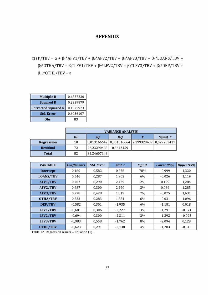
71

APPENDIX

(1) P/TBV = α + β1*AFV1/TBV + β2*AFV2/TBV + β3*AFV3/TBV + β4*LOANS/TBV +

β5*OTHA/TBV + β6*LFV1/TBV + β7*LFV2/TBV + β8*LFV3/TBV + β9*DEP/TBV +

β10*OTHL/TBV + ε

Multiple R 0,4837230

Squared R 0,2339879

Corrected squared R 0,1275973

Std. Error 0,6036107

Obs. 83

VARIANCE ANALYSIS

DF SQ MQ F Signif. F

Regression 10 8,013166642 0,801316664 2,199329437 0,027233417

Residual 72 26,23290483 0,3643459

Total 82 34,24607148

VARIABLE Coefficients Std. Error Stat. t Signif. Lower 95% Upper 95%

Intercept 0,160 0,582 0,276 78% -0,999 1,320

LOANS/TBV 0,546 0,287 1,902 6% -0,026 1,119

AFV1/TBV 0,707 0,290 2,439 2% 0,129 1,284

AFV2/TBV 0,687 0,300 2,290 2% 0,089 1,285

AFV3/TBV 0,778 0,428 1,819 7% -0,075 1,631

OTHA/TBV 0,533 0,283 1,884 6% -0,031 1,096

DEP/TBV -0,582 0,301 -1,935 6% -1,181 0,018

LFV1/TBV -0,681 0,306 -2,227 3% -1,291 -0,071

LFV2/TBV -0,694 0,300 -2,311 2% -1,292 -0,095

LFV3/TBV -0,983 0,558 -1,762 8% -2,094 0,129

OTHL/TBV -0,623 0,291 -2,138 4% -1,203 -0,042

Table 12. Regression results – Equation (1).

72

(2) Pi/TBV i = α + β1*AFV1 i/TBV i + β2*AFV2 i/TBV i + β3*AFV3 i/TBV i + β4*LOANS i/TBV i +

β5*OTHA i/TBV i + β6*LFV1 i/TBV i + β7*LFV2 i/TBV i + β8*LFV3 i/TBV i + β9*DEPi/TBV i +

β10*OTHL i/TBV i + β11*YEAR + ε


Squared R 0,2946485



Obs. 83

VARIANCE ANALYSIS


Regression 11 10,09055 0,917323 2,696276 0,00588334

Residual 71 24,15552 0,340219

Total 82 34,24607

VARIABLE Coefficients Std. Error Stat t Signif. Lower 95% Upper 95%

Intercept 0,577 0,587 0,984 33% -0,593 1,748

YEAR -0,326 0,132 -2,471 2% -0,589 -0,063

LOANS/TBV 0,418 0,282 1,481 14% -0,145 0,981

AFV1/TBV 0,566 0,286 1,983 5% -0,003 1,136

AFV2/TBV 0,550 0,295 1,862 7% -0,039 1,138

AFV3/TBV 0,609 0,419 1,453 15% -0,227 1,445

OTHA/TBV 0,405 0,278 1,458 15% -0,149 0,960

DEP/TBV -0,449 0,296 -1,519 13% -1,038 0,140

LFV1/TBV -0,546 0,301 -1,818 7% -1,146 0,053

LFV2/TBV -0,551 0,296 -1,863 7% -1,141 0,039

LFV3/TBV -0,856 0,541 -1,581 12% -1,935 0,223

OTHL/TBV -0,491 0,286 -1,713 9% -1,062 0,080


73

(3) Pi/TBV i = α + β1*AFV1 i/TBV i + β2*AFV2 i/TBV i + β3*AFV3 i/TBV i + β4*LOANS i/TBV i +

β5*OTHA i/TBV i + β6*LFV1 i/TBV i + β7*LFV2 i/TBV i + β8*LFV3 i/TBV i + β9*DEPi/TBV i +

β10*OTHL i/TBV i + β10*ROTEi + β11*YEAR + ε


Squared R 0,3407836



Obs. 83

VARIANCE ANALYSIS


Regression 12 11,67049905 0,972541588 3,015556366 0,00187011

Residual 70 22,57557242 0,322508177

Total 82 34,24607148

VARIABLES Coefficients Std. Error Stat t Signif. Lower 95% Upper 95%

Intercept 0,456 0,574 0,794 43% -0,689 1,601

ROTE 1,256 0,567 2,213 3% 0,124 2,387

YEAR -0,231 0,136 -1,707 9% -0,502 0,039

LOANS/TBV 0,413 0,275 1,503 14% -0,135 0,961

AFV1/TBV 0,544 0,278 1,953 5% -0,012 1,099

AFV2/TBV 0,511 0,288 1,774 8% -0,063 1,085

AFV3/TBV 0,512 0,410 1,247 22% -0,307 1,331

OTHA/TBV 0,396 0,271 1,463 15% -0,144 0,936

DEP/TBV -0,441 0,288 -1,531 13% -1,014 0,133

LFV1/TBV -0,511 0,293 -1,742 9% -1,095 0,074

LFV2/TBV -0,509 0,289 -1,763 8% -1,084 0,067

LFV3/TBV -0,864 0,527 -1,639 11% -1,915 0,187

OTHL/TBV -0,477 0,279 -1,711 9% -1,034 0,079


74

LEVEL/TOT. FV ASSETS LEVEL/TOT. FV LIABILITIES

BANK A.L1/TOT A.L2/TOT A.L3/TOT L.L1/TOT L.L2/TOT L.L3/TOT

Banca Monte dei Paschi di Siena S.p.A. 49,19% 49,79% 1,02% 1,43% 98,40% 0,17%

Banca Popolare dell'Emilia Romagna S.C.A.R.L. 71,99% 15,57% 12,43% 0,02% 98,13% 1,85%

Banca Popolare di Milano S.C.A.R.L. 73,11% 19,43% 7,46% 6,13% 90,84% 3,03%

Banco Bilbao Vizcaya Argentaria S.A. 58,14% 40,69% 1,17% 12,49% 87,45% 0,06%

Banco de Sabadell S.A. 75,70% 22,03% 2,28% 0,00% 86,75% 13,25%

Banco Espirito Santo S/A 39,02% 59,86% 1,12% 0,00% 100,00% 0,00%

Banco Popolare S.C. 69,80% 26,72% 3,49% 59,40% 40,60% 0,01%

Banco Popular Espanol S.A. 77,75% 13,45% 8,80% 0,68% 62,88% 36,43%

Banco Santander S.A. 49,89% 49,36% 0,75% 11,08% 88,78% 0,14%

Bank of Ireland Ord Stk EUR0.64 73,79% 25,33% 0,88% 0,00% 96,59% 3,41%

Barclays PLC 11,86% 83,97% 4,17% 5,70% 92,57% 1,73%

BNP Paribas S.A. 35,96% 60,95% 3,09% 16,69% 78,65% 4,65%

Commerzbank AG 18,40% 79,60% 2,00% 9,54% 89,88% 0,58%

Credit Agricole S.A. 48,11% 49,85% 2,04% 8,56% 90,34% 1,09%

Credit Suisse Group AG 41,08% 50,24% 8,69% 25,47% 67,35% 7,18%

Danske Bank A/S 37,39% 61,70% 0,91% 65,23% 33,94% 0,83%

Deutsche Bank AG 11,80% 84,19% 4,01% 6,59% 91,90% 1,51%

DNB ASA 40,40% 35,87% 23,72% 0,00% 99,92% 0,08%

Erste Group Bank AG 43,53% 55,76% 0,71% 1,23% 98,75% 0,02%

HSBC Holdings PLC 43,66% 54,60% 1,74% 22,99% 74,57% 2,44%

Intesa Sanpaolo S.p.A. 60,93% 37,06% 2,01% 10,04% 88,90% 1,06%

Julius Baer Gruppe AG 50,40% 49,60% 0,00% 46,66% 53,34% 0,00%

Jyske Bank A/S 69,87% 29,30% 0,83% 1,77% 98,23% 0,00%

KBC Group N.V. 67,19% 28,22% 4,59% 12,83% 69,68% 17,48%

Lloyds Banking Group PLC 51,50% 45,51% 2,99% 1,31% 98,31% 0,37%

Mediobanca Banca di Credito Finanziario 59,68% 31,99% 8,33% 19,33% 67,37% 13,31%

National Bank of Greece S.A. 28,99% 69,59% 1,41% 0,23% 99,46% 0,30%

Natixis 32,83% 60,06% 7,11% 16,44% 82,97% 0,60%

Nordea Bank AB 26,10% 70,77% 3,13% 19,66% 79,20% 1,14%

Pohjola Bank Plc 65,48% 31,45% 3,07% 1,17% 96,11% 2,72%

Raiffeisen Bank International AG 52,48% 46,64% 0,88% 16,48% 83,52% 0,00%

Royal Bank of Scotland Group Plc 16,60% 81,40% 2,00% 5,53% 93,72% 0,75%

Skandinaviska Enskilda Banken AB 38,01% 59,96% 2,04% 31,61% 59,49% 8,90%

Societe Generale 42,83% 54,24% 2,93% 4,16% 89,50% 6,34%

Standard Chartered PLC 35,85% 62,54% 1,61% 9,64% 89,48% 0,88%

Svenska Handelsbanken A 59,64% 39,18% 1,17% 47,12% 52,78% 0,10%

Swedbank AB 24,01% 75,91% 0,08% 25,82% 74,17% 0,00%

Sydbank A/S 4,68% 93,71% 1,62% 0,12% 99,88% 0,00%

UBS AG 24,97% 71,50% 3,53% 8,17% 87,47% 4,35%

UniCredit S.p.A. 38,61% 56,56% 4,83% 10,38% 86,64% 2,98%

Unione di Banche Italiane SCpA 80,37% 18,01% 1,62% 18,79% 81,21% 0,00%

Table 15. First three columns: shares of level 1, level 2, level 3 assets on total fair value assets. Last

three columns: shares of level 1, level 2, level 3 liabilities on total fair value liabilities. (data from

2010 annual reports)

75

LEVEL/TOTAL FV ASSETS LEVEL/TOTAL FV LIABILITIES

BANK A.L1/TOT A.L2/TOT A.L3/TOT L.L1/TOT L.L2/TOT L.L3/TOT

Banca Monte dei Paschi di Siena S.p.A. 49,55% 49,56% 0,90% 3,70% 96,21% 0,09%

Banca Popolare dell'Emilia Romagna S.C.A.R.L. 75,55% 13,43% 11,02% 0,00% 98,53% 1,47%

Banca Popolare di Milano S.C.A.R.L. 67,85% 24,21% 7,94% 2,07% 94,99% 2,93%

Banco Bilbao Vizcaya Argentaria S.A. 49,30% 49,40% 1,30% 10,41% 89,55% 0,04%

Banco de Sabadell S.A. 77,99% 20,16% 1,85% 3,91% 83,27% 12,82%

Banco Espirito Santo S/A 30,26% 68,27% 1,46% 0,00% 100,00% 0,00%

Banco Popolare S.C. 64,73% 32,41% 2,86% 51,30% 48,70% 0,00%

Banco Popular Espanol S.A. 75,63% 15,96% 8,42% 0,00% 93,84% 6,16%

Banco Santander S.A. 40,76% 58,88% 0,36% 8,39% 91,47% 0,14%

Bank of Ireland Ord Stk EUR0.64 69,28% 27,78% 2,94% 0,02% 97,31% 2,67%

BANKIA S.A. 46,08% 46,80% 7,13% 1,86% 98,14% 0,00%

Barclays PLC 12,44% 83,54% 4,02% 4,30% 93,93% 1,77%

BNP Paribas S.A. 27,15% 69,63% 3,22% 14,43% 81,21% 4,36%

CaixaBank S.A. 64,50% 33,38% 2,13% 15,57% 84,39% 0,04%

Commerzbank AG 24,96% 72,81% 2,23% 8,27% 91,02% 0,71%

Credit Agricole S.A. 36,87% 61,08% 2,06% 6,69% 92,76% 0,55%

Credit Suisse Group AG 35,34% 55,93% 8,74% 22,19% 71,82% 5,99%

Danske Bank A/S 34,67% 64,05% 1,28% 54,74% 43,83% 1,43%

Deutsche Bank AG 9,53% 86,90% 3,57% 4,65% 94,05% 1,30%

DNB ASA 16,69% 66,29% 17,02% 0,00% 99,94% 0,06%

Erste Group Bank AG 42,63% 56,91% 0,47% 0,74% 99,24% 0,02%

HSBC Holdings PLC 38,80% 59,44% 1,75% 18,33% 80,01% 1,65%

Intesa Sanpaolo S.p.A. 57,80% 40,16% 2,04% 5,31% 93,48% 1,21%

Julius Baer Gruppe AG 62,41% 37,59% 0,00% 24,49% 75,51% 0,00%

Jyske Bank A/S 56,26% 42,83% 0,91% 1,05% 98,95% 0,00%

KBC Group N.V. 61,37% 30,05% 8,57% 13,15% 67,78% 19,07%

Lloyds Banking Group PLC 52,94% 43,91% 3,15% 3,85% 95,20% 0,95%

Mediobanca Banca di Credito Finanziario S.p.A. 61,14% 28,11% 10,74% 38,92% 45,44% 15,64%

Natixis 23,32% 72,81% 3,87% 12,29% 87,63% 0,08%

Nordea Bank AB 23,55% 74,57% 1,88% 14,63% 84,92% 0,45%

Pohjola Bank Plc 58,22% 39,35% 2,43% 0,69% 96,53% 2,77%

Raiffeisen Bank International AG 49,87% 49,52% 0,60% 4,84% 94,35% 0,81%

Royal Bank of Scotland Group Plc 14,44% 83,70% 1,86% 4,60% 94,56% 0,83%

Skandinaviska Enskilda Banken AB 35,19% 63,94% 0,87% 26,49% 71,50% 2,00%

Societe Generale 34,85% 62,86% 2,28% 3,73% 91,05% 5,23%

Standard Chartered PLC 29,81% 68,25% 1,94% 6,01% 93,58% 0,42%

Svenska Handelsbanken A 51,98% 47,47% 0,55% 39,08% 60,89% 0,04%

Swedbank AB 23,15% 76,80% 0,05% 27,52% 72,48% 0,00%

Sydbank A/S 3,61% 94,86% 1,53% 0,07% 99,93% 0,00%

UBS AG 19,41% 77,08% 3,51% 5,50% 90,70% 3,80%

UniCredit S.p.A. 26,74% 67,93% 5,33% 6,44% 90,42% 3,14%

Unione di Banche Italiane SCpA 75,57% 22,72% 1,71% 15,63% 84,37% 0,00%

Table 16. First three columns: shares of level 1, level 2, level 3 assets on total fair value assets. Last

three columns: shares of level 1, level 2, level 3 liabilities on total fair value liabilities (data from 2011

annual reports).

76

2010 2011

BANK FVA/TA FVL/TL FVA/TA FVL/TL

Banca Monte dei Paschi di Siena S.p.A. 23,04% 25,39% 23,20% 23,15%

Banca Popolare dell'Emilia Romagna 7,39% 5,30% 8,17% 7,81%

Banca Popolare di Milano S.C.A.R.L. 22,75% 3,73% 20,87% 5,84%

Banco Bilbao Vizcaya Argentaria S.A. 22,72% 7,86% 22,71% 10,01%

Banco de Sabadell S.A. 12,33% 1,27% 14,64% 1,53%

Banco Espirito Santo S/A 22,68% 15,70% 22,39% 19,56%

Banco Popolare S.C. 13,01% 24,74% 14,44% 24,60%

Banco Popular Espanol S.A. 10,69% 1,68% 9,69% 2,05%

Banco Santander S.A. 23,88% 18,03% 23,07% 17,01%

Bank of Ireland Ord Stk EUR0.64 19,22% 12,75% 16,51% 14,11%

BANKIA S.A. - - 27,10% 9,95%

Barclays PLC 46,71% 40,35% 50,95% 44,17%

BNP Paribas S.A. 52,97% 38,36% 52,03% 41,34%

CaixaBank S.A. - - 22,13% 5,62%

Commerzbank AG 39,06% 30,63% 36,63% 30,96%

Credit Agricole S.A. 41,60% 23,95% 43,58% 28,33%

Credit Suisse Group AG 56,52% 42,77% 51,49% 40,35%

Danske Bank A/S 53,03% 35,42% 58,15% 40,16%

Deutsche Bank AG 61,07% 46,37% 61,62% 48,94%

DNB ASA 29,12% 30,05% 32,14% 33,51%

Erste Group Bank AG 16,34% 4,56% 18,30% 5,86%

HSBC Holdings PLC 43,35% 28,15% 42,52% 29,14%

Intesa Sanpaolo S.p.A. 26,78% 12,76% 27,10% 13,52%

Julius Baer Gruppe AG 45,14% 18,50% 34,70% 13,21%

Jyske Bank A/S 38,57% 17,15% 35,55% 16,25%

KBC Group N.V. 33,87% 19,69% 28,07% 21,41%

Lloyds Banking Group PLC 25,20% 7,30% 25,03% 9,01%

Mediobanca Banca di Credito Finanziario S.p.A. 32,95% 9,79% 30,05% 11,84%

National Bank of Greece 15,65% 3,89% - -

Natixis 42,61% 36,46% 55,99% 47,96%

Nordea Bank AB 45,58% 35,56% 52,13% 39,98%

Pohjola Bank Plc 28,27% 6,08% 30,81% 8,92%

Raiffeisen Bank International AG 13,50% 7,92% 15,56% 10,18%

Royal Bank of Scotland Group Plc 54,08% 46,52% 58,55% 52,84%

Skandinaviska Enskilda Banken AB 23,06% 10,67% 22,89% 11,35%

Societe Generale 49,38% 33,20% 46,32% 34,97%

Standard Chartered PLC 28,23% 14,11% 28,80% 15,34%

Svenska Handelsbanken A 14,76% 10,04% 13,44% 9,29%

Swedbank AB 51,52% 26,44% 47,22% 22,91%

Sydbank A/S 46,24% 27,73% 48,19% 32,61%

UBS AG 52,71% 44,86% 50,23% 45,42%

UniCredit S.p.A. 23,25% 14,51% 25,22% 15,74%

Unione di Banche Italiane SCpA 10,51% 1,84% 9,34% 2,34%

Table 17. Shares of fair value assets (fair value liabilities) on total assets (total liabilities).

ifrs enforcement for banks: the case of value relevance of the fair value hierarchy

Documents

tesi di dottorato

mortgage servicing rights

bad debts provision

tangible equity ratio

effective interest method

future cash flows

observed market prices

ante information quality