ieor e4602: quantitative risk management spring 2016 2016...
TRANSCRIPT

IEOR E4602: Quantitative Risk Management Spring 2016c© 2016 by Martin Haugh
Basic Concepts and Techniques of RiskManagement
We introduce the basic concepts and techniques of risk management in these lecture notes. We will closelyfollow the content and notation of Chapter 2 of Quantitative Risk Management by McNeil, Frey and Embrechts.This chapter should be consulted if further details are required.
1 Risk Factors and Loss Distributions
Let ∆ be a fixed period of time such as 1 day or 1 week. This will be the horizon of interest when it comes tomeasuring risk and calculating loss distributions. Let Vt be the value of a portfolio at time t∆ so that theportfolio loss between times t∆ and (t+ 1)∆ is given by
Lt+1 := − (Vt+1 − Vt) . (1)
Note that we treat a loss as a positive quantity so, for example, a negative value of Lt+1 denotes a profit. Thetime1 t value of the portfolio depends of course on the time t value of the securities in the portfolio. Moregenerally, however, we may wish to define a set of d risk factors, Zt := (Zt,1, . . . , Zt,d) so that Vt is a functionof t and Zt. That is
Vt = f(t,Zt)
for some function f : R+ × Rd → R. In a stock portfolio, for example, we might take the stock prices or somefunction of the stock prices as our risk factors. In an options portfolio, however, Zt might contain stock factorstogether with implied volatility and interest rate factors. Now let Xt := Zt − Zt−1 denote the change in thevalues of the risk factors between times t and t− 1. Then we have
Lt+1(Xt+1) = − (f(t+ 1,Zt + Xt+1)− f(t,Zt)) (2)
and given the value of Zt, the distribution of Lt+1 then depends only on the distribution of Xt+1.
1.1 Linear Approximations to the Loss Function
Assuming f(·, ·) is differentiable, we can use a first order Taylor expansion to approximate Lt+1 with
L̂t+1(Xt+1) := −
(ft(t,Zt)∆ +
d∑i=1
fzi(t,Zt) Xt+1,i
)(3)
where the f -subscripts denote partial derivatives. The first order approximation is commonly used when Xt+1 islikely to be small. This is often the case when ∆ is small, e.g. 1/365 ≡ 1 day, and the market is not too volatile.Second and higher order approximations also based on Taylor’s Theorem can also be used. It is important tonote, however, that if Xt+1 is likely to be very large then Taylor approximations of any order are likely to workpoorly if at all.
1When we say time t we typically have in mind time t∆.

Basic Concepts and Techniques of Risk Management 2
1.2 Conditional and Unconditional Loss Distributions
When we discuss the distribution of L̂t+1 it is important to clarify exactly what we mean. In particular, we needto distinguish between the conditional and unconditional loss distributions. Consider the series Xt of risk factorchanges and assume that they form a stationary2 time series with stationary distribution FX. We also let Ftdenote all information available in the system at time t, including {Xs : s ≤ t} in particular. We then have thefollowing two definitions.
Definition 1 The unconditional loss distribution is the distribution of Lt+1 given the time t composition ofthe portfolio and assuming the CDF of Xt+1 is given by FX.
Definition 2 The conditional loss distribution is the distribution of Lt+1 given the time t composition of theportfolio and conditional on the information in Ft.
It is clear that if the Xt’s are IID then the conditional and unconditional distributions coincide. For long timehorizons, e.g. ∆ = 6 months, we might be more inclined to use the unconditional loss distribution. However, forshort horizons, e.g. 1 day or 10 days, then the conditional loss distribution is clearly the appropriate distribution.This would be particularly true in times of high market volatility when the unconditional distribution would bearlittle resemblance to the true conditional distribution.
Example 1 (A Stock Portfolio)Consider a portfolio of d stocks with St,i denoting the time t price of the ith stock and λi denoting the numberof units of this stock in the portfolio. If we take log stock prices as our factors then we obtain
Xt+1,i = lnSt+1,i − lnSt,i
and
Lt+1 = −d∑i=1
λiSt,i(eXt+1,i − 1
).
The linear approximation satisfies
L̂t+1 = −d∑i=1
λiSt,iXt+1,i = −Vtd∑i=1
ωt,iXt+1,i
where ωt,i := λiSt,i/Vt is the ith portfolio weight. If Xt+1,i has mean vector µ and variance-covariance matrix
Σ then we obtain Et[L̂t+1
]= −Vtω′µ and Vart
(L̂t+1
)= V 2
t ω′Σω. Note that µ and Σ could refer to the
first two moments of either the conditional or unconditional loss distribution.
Example 2 (An Options Portfolio)The Black-Scholes formula for the time t price of a European call option with strike K and maturity T on anon-dividend paying stock satisfies
C(St, t, σ) = StΦ(d1) − e−r(T−t)KΦ(d2)
where d1 =log(St
K
)+ (r + σ2/2)(T − t)σ√T − t
, d2 = d1 − σ√T − t
Φ(·) is the CDF of the standard normal distribution, St is the time t price of the underlying security and r is therisk-free interest rate. While the Black-Scholes model assumes a constant volatility, σ, in practice an impliedvolatility, σ(K,T, t), that depends on the strike, maturity and current time, t, is observed in the market.
Consider now a portfolio of European options all on the same underlying security. The portfolio may alsocontain a position in the underlying security itself. If the portfolio contains d different options with a position of
2A time series, Xt, is strongly stationary if (Xt1 , . . . ,Xtn ) is equal in distribution to (Xt1+k, . . . ,Xtn+k) for alln, k, t1, . . . , tn ∈ Z+. Most risk factors are assumed to be stationary.

Basic Concepts and Techniques of Risk Management 3
λi in the ith option, then
Lt+1 = −λ0(St+1 − St) −d∑i=1
λi (C(St+1, t+ 1, σ(Ki, Ti, t+ 1)− C(St, t, σ(Ki, Ti, t))) (4)
where λ0 is the position in the underlying security. Note that by put-call parity we can assume that all optionsare call options. We can also use the linear approximation technique to approximate Lt+1 in (4). This wouldresult in a delta-vega-theta approximation. For derivatives portfolios, the linear approximation technique basedon the first-order Greeks is often inadequate and second order approximations involving gamma and possiblyvolga and vanna are often employed.
For risk factors, we can again take the log stock prices but it is not clear how to handle the implied volatilities.There are several possibilities:
1. One possibility is to assume that the σ(K,T, t)’s simply do not change. This is not very satisfactory but iscommonly assumed when historical simulation3 is used to approximate the loss distribution and historicaldata on the changes in implied volatilities are not available.
2. Let each σ(K,T, t) be a separate factor. In addition to approximately doubling the number of factors, aparticular problem with this approach is that the implied volatilities are not free to move aroundindependently. In fact the assumption of no-arbitrage imposes strong restrictions on how the impliedvolatility surface may move. It is therefore important to choose factors in such a way that thoserestrictions are easily imposed when we estimate the loss distribution.
3. There are d implied volatilities to consider and in principal this leads to d factors, albeit with restrictionson how these factors can move. We could use dimension reduction techniques such as principalcomponents analysis (PCA) to identify just two or three variables that explain most of the movements inthe volatility surface.
4. As an alternative to PCA, we could parameterize the volatility surface with just a few parameters andassume that only those parameters can move from one period to the next. The parameterization shouldbe such that the no-arbitrage restrictions are easy to enforce. The obvious candidates would be factorsthat represent the level, term structure and skew of the implied volatility surface.
Example 3 (A Bond Portfolio)Consider a portfolio containing quantities of d different default-free zero-coupon4 bonds where the ith bond hasprice Pt,i, maturity Ti and face value equal5 to 1. Let st,Ti
denote the continuously compounded spot interestrate for maturity Ti so that
Pt,i = exp(−st,Ti(Ti − t)).If there are λi units of the ith bond in the portfolio, then the total portfolio value is given by
Vt =
d∑i=1
λi exp(−st,Ti(Ti − t)).
Assume now that we only consider the possibility of parallel changes in the spot rate curve. Then if the spotcurve moves by δ the portfolio loss satisfies
Lt+1 = −d∑i=1
λi (exp(−(st+∆,Ti + δ)(Ti − t−∆)) − exp(−st,Ti(Ti − t)))
≈ −d∑i=1
λi (st,Ti(Ti − t) − (st+∆,Ti
+ δ)(Ti − t−∆)) . (5)
3See Section 3.4There is no loss of generality here since we can decompose a default-free coupon bond into a series of zero-coupon bonds.5There is also no loss of generality in assuming a face value of 1 since we can compensate by adjusting the quantity of each
bond in the portfolio.

Basic Concepts and Techniques of Risk Management 4
We therefore have a single risk factor, δ, that we can use to study the distribution of the portfolio loss. Notethat if we assume that ∆ is small so that st+∆,Ti
≈ st,Tithen we can further approximate the right-hand-side of
(5) to obtain
Lt+1 ≈ δ
d∑i=1
λi(Ti − t). (6)
We can use (how?) (5) or (6) to hedge parallel changes in the spot rate curve. Note that this is equivalent tohedging using the Fisher-Weil duration of the portfolio. Had we used a second-order approximation to theexponential function in deriving (5) then we would introduce the standard concept of convexity.
While hedging against parallel shifts in the spot rate curve often leads to good results, in practice the spot ratecurve tends to move in a non-parallel manner and more sophisticated6 hedging techniques produce superiorresults.
2 Risk Measurement
2.1 Approaches to Risk Measurement
We now outline several approaches to the problem of risk measurement.
Notional Amount Approach
This approach to risk management defines the risk of a portfolio as the sum of the notional amounts of theindividual positions in the portfolio. Each notional amount may be weighted by a factor representing theperceived riskiness of the position. While it is simple, it has many weaknesses. It does not reflect the benefits ofdiversification, does not allow for any netting and does not distinguish between long and short positions.Moreover, it is not always clear what the notional amount of a derivative is and so the notional approach can bedifficult to apply when such derivatives are present in the portfolio.
Factor Sensitivity Measures
A factor sensitivity measure gives the change in the value of the portfolio for a given change in the factor.Commonly used examples include the Greeks of an option portfolio or the duration and convexity of a bondportfolio. These measures are often used to set position limits on trading desks and portfolios. They aregenerally not used for capital adequacy decisions as it is often difficult to aggregate these measures acrossdifferent risk factors and markets.
For an example consider an option with time t price C that is written on an underlying security with priceprocess St. We assume the time t price, C, is a function of only St and the implied volatility, σt. Then a simpleapplication of Taylor’s Theorem yields
C(S + ∆S, σ + ∆σ) ≈ C(S, σ) + ∆S∂C
∂S+
1
2(∆S)2 ∂
2C
∂S2+ ∆σ
∂C
∂σ
= C(S, σ) + ∆S δ +1
2(∆S)2 Γ + ∆σ vega.
where we have omitted the dependence of the various quantities on t. We therefore obtain
P&L ≈ δ∆S +Γ
2(∆S)2 + vega ∆σ
= delta P&L + gamma P&L + vega P&L . (7)
6For example, methods based on principal components analysis (PCA) are often used in practice. We will study PCA whenwe study dimension reduction techniques.

Basic Concepts and Techniques of Risk Management 5
When ∆σ = 0, we obtain obtain the well-known delta-gamma approximation which is often used, forexample, in historical Value-at-Risk (VaR) calculations. Note that we can also write (7)
P&L ≈ δS
(∆S
S
)+
ΓS2
2
(∆S
S
)2
+ vega ∆σ
= ESP× Return + $ Gamma× Return2 + vega ∆σ (8)
where ESP denotes the equivalent stock position or “dollar” delta. Note that it is easy to extend thiscalculation to a portfolio of options on the same underlying security. It is also straightforward7 to extend theseideas to derivatives portfolios written with many different underlying securities.
Depending on the particular asset class, investors / traders / risk managers should always know their exposureto the Greeks, i.e. dollar delta, dollar gamma and vega etc. It is also very important to note that approximationssuch as (8) are local approximations as they are based (via Taylor’s Theorem) on “small” moves in the riskfactors. These approximations can and indeed do break down in violent markets where changes in the riskfactors can be very large.
Scenario or Stress Approach
The scenario approach defines a number of scenarios where in each scenario the various risk factors are assumedto have moved by some fixed amounts. For example, a scenario might assume that all stock prices have fallen by10% and all implied volatilities have increased by 5 percentage points. Another scenario might assume the samemovements but with an additional steepening of the volatility surface. A scenario for a credit portfolio mightassume that all credit spreads have increased by some fixed absolute amount, e.g. 100 basis points, or some fixedrelative amount, e.g. 10%. The risk of a portfolio could then be defined as the maximum loss over all of thescenarios that were considered. A particular advantage of this approach is that it does not depend on probabilitydistributions that are difficult to estimate. In that sense, the scenario approach to risk management isvery robust and should play a vital role in any financial risk management operation.
Figure 1: P&L for an Options Portfolio on SP5X under Stresses to Underlying and Implied Volatility
Figure 1 shows the P&L under various scenarios of an options portfolio with the S&P500 as the underlyingsecurity. The vertical axis represents percentage shifts in the price of the underlying security whereas thehorizontal axis represents absolute changes in the implied volatility of each option in the portfolio. For example,we see that if the S&P500 were to fall by 20% and implied volatilities were to all rise by 5 percentage points,then the portfolio would gain 8.419 million dollars (assuming that the numbers in Figure 1 are expressed in units
7And we shall do this when we discuss dimension reduction methods in a later set of lecture notes.
Basic Concepts and Techniques of Risk Management 6
of 1, 000 dollars). When constructing scenario tables as in 1 we can use approximations like (8) to check forinternal consistency and to help identify possible bugs in the software.
While scenario tables are a valuable source of information there are many potential pit-falls associated withusing them. These include:
1. Identifying the relevant risk factors
While it is usually pretty clear what the main risk factors for a particular asset class are, it is quite possiblethat a portfolio has been constructed so that it is approximately neutral to changes in those risk factors.Such a portfolio might then only have (possibly very large) exposures to secondary risk factors. It isimportant then to include shifts in these secondary factors in any scenario analysis. The upshot is that thethe relevant risk factors depend on the specific portfolio under consideration rather than just the assetclass of the portfolio.
2. Identifying “reasonable” shifts for these risk factors
For example, we may feel that a shift of −10% is plausible for the S&P 500 because we know fromexperience that such a move, while extreme, is indeed possible in a very volatile market. But how do wedetermine plausible shifts for less transparent risk factors? The answer typically lies in the use of statisticaltechniques such as PCA, extreme-value theory, time series methods, common sense(!) etc.
A key role of any risk manager then is to understand what scenarios are plausible and what scenarios are not.For example, in a crisis we would expect any drop in the price of the underlying security to be accompanied by arise in implied volatilities. We would therefore pay considerably less attention to the numbers in the upper leftquadrant of Figure 1.
Measures Based on Loss Distribution
Many risk measures such as value-at-risk (VaR) or conditional value-at-risk (CVaR) are based on the lossdistribution of the portfolio. Working with loss distributions makes sense as the distribution contains all theinformation you could possibly wish to know about possible losses. A loss distribution implicitly reflects thebenefits of netting and diversification. Moreover it is easy to compare the loss distribution of a derivativesportfolio with that of a bond or credit portfolio, at least when the same time horizon is under consideration.However, it must be noted that it may be very difficult to estimate the loss distribution. This may be the casefor a number of reasons including a lack of historical data, non-stationarity of risk-factors and poor model choiceamong others.
2.2 Value-at-Risk
Value-at-Risk (VaR) is the most widely used risk measure in the financial industry. Despite the many weaknessesof VaR, financial institutions are required to use it under the Basel II capital-adequacy framework. In addition,many institutions routinely report their VaR numbers to shareholders, investors or regulatory authorities. VaR isa risk measure based on the loss distribution and our discussion will not depend on whether we are dealing withthe conditional or unconditional loss distribution. Nor will it depend on whether we are using the true lossdistribution or some approximation to it. We will assume that the horizon, ∆, has been fixed and that therandom variable L represents the loss on the portfolio under consideration over the time interval ∆. We will useFL(·) to denote the cumulative distribution function (CDF) of L. We first define the quantiles of a CDF.
Definition 3 Let F : R→ [0, 1] be an arbitrary CDF. Then for α ∈ (0, 1) the α-quantile of F is defined by
qα(F ) := inf{x ∈ R : F (x) ≥ α}.
Note that if F is continuous and strictly increasing, then qα(F ) = F−1(α). For a random variable L with CDFFL(·), we will often write qα(L) instead of qα(FL). Using the fact that any CDF is by definitionright-continuous, we immediately obtain the following result.
Lemma 1 A point x0 ∈ R is the α-quantile of FL if and only if (i) FL(x0) ≥ α and (ii) FL(x) < α for allx < x0.

Basic Concepts and Techniques of Risk Management 7
Definition 4 Let α ∈ (0, 1) be some fixed confidence level. Then the VaR of the portfolio loss at theconfidence level, α, is given by VaRα := qα(L), the α-quantile of the loss distribution.
Example 4 (The Normal and t Distributions)Because the normal and t CDFs are both continuous and strictly increasing, it is straightforward to calculatetheir VaRα. If L ∼ N(µ, σ2) then
VaRα = µ+ σΦ−1(α) where Φ is the standard normal CDF. (9)
By the previous lemma, this follows if we can show that FL(VaRα) = α. But this follows immediately from (9).
If L ∼ t(ν, µ, σ2) so that (L− µ)/σ has a standard t distribution with ν > 2 degrees-of-freedom, then
VaRα = µ+ σt−1ν (α) where tν is the CDF for the t distribution with ν degrees-of-freedom.
Note that in this case we have E[L] = µ and Var(L) = νσ2/(ν − 2).
VaR has several weaknesses:
1. VaR attempts to describe the entire loss distribution with a single number and so significant information isnot captured in VaR. This criticism does of course apply to all scalar risk measures. One way around thisis to report VaRα for several different values of α.
2. There is significant model risk attached to VaR. If the loss distribution is heavy-tailed, for example, but anormal distribution is assumed, then VaRα will be severely underestimated as α approaches 1. Afundamental problem with VaR and other risk measures based on the loss distribution is that it can bevery difficult to estimate the loss distribution. Even when there is sufficient historical data available thereis no guarantee that the historical data-generating process will remain unchanged in the future. Forexample, in the buildup to the sub-prime housing crisis it was clear that the creation and selling of vastquantities of structured credit products could change the price dynamics of these and related securities.And of course, that is precisely what happened.
3. VaR is not a sub-additive risk measure so that it doesn’t lend itself to aggregation. For example, letL = L1 +L2 be the total loss associated with two portfolios, each with respective losses, L1 and L2. Then
qα(FL) > qα(FL1) + qα(FL2) is possible. (10)
In the risk literature this is viewed as being an undesirable property as we would expect somediversification benefits when we combine two portfolios together. Such a benefit would be reflected by thecombined portfolio having a smaller risk measure than the sum of the two individual risk measures.
An advantage of VaR is that it is generally easier8 to estimate. This is true when it comes to quantileestimation in general as quantiles are not very sensitive to outliers. This is not true of other risk measures suchas CVaR which we discuss below. Despite this fact, it becomes progressively more difficult to estimate VaRα asα gets closer to 1. Extreme Value Theory (EVT) can be useful in these circumstances, however, and we willreturn to EVT in later lectures.
The value of ∆ that we use in practice generally depends on the application. For credit, operational andinsurance risk, ∆ is often on the order of 1 year. For financial risks, however, typical values of ∆ are on theorder of days, with 1 and 10 days being very common.
8This assumes of course that we have correctly specified the appropriate probability model so that the second weaknessabove is not an issue. This assumption is often not justified!
Basic Concepts and Techniques of Risk Management 8
2.3 Expected Shortfall (ES) / Conditional Value-at-Risk (CVaR)
We now define expected shortfall which is also commonly referred to as conditional value-at-risk (CVaR).
Definition 5 For a portfolio loss, L, satisfying E[|L|] <∞ the expected shortfall at confidence level α ∈ (0, 1)is given by
ESα :=1
1− α
∫ 1
α
qu(FL) du.
The relationship between ESα and VaRα is therefore given by
ESα :=1
1− α
∫ 1
α
VaRu(L) du
from which it is clear that ESα(L) ≥ VaRα(L). A more well known representation of ESα(L) holds when FL iscontinuous.
Lemma 2 If FL is a continuous CDF then
ESα :=E [L; L ≥ qα(L)]
1− α= E [L | L ≥ VaRα] . (11)
Proof: See Lemma 2.13 in McNeil, Frey and Embrechts. The proof is straightforward and relies on thestandard result that the random variable F−1
L (U) has distribution FL when U ∼ Uniform(0, 1).
Example 5 (Expected Shortfall for a Normal Distribution)
We can use (11) to compute the expected shortfall of an N(µ, σ2) random variable. In particular we can checkthat
ESα = µ + σφ(Φ−1(α)
)1− α
(12)
where φ(·) is the PDF of the standard normal distribution.
Example 6 (Expected Shortfall for a t Distribution)
Let L ∼ t(ν, µ, σ2) so that L̃ := (L− µ)/σ has a standard t distribution with ν > 2 degrees-of-freedom. Thenas in the previous example it is easy to see that ESα(L) = µ+ σESα(L̃). It is straightforward using directintegration to check that
ESα(L̃) =gν(t−1ν (α)
)1− α
(ν + (t−1
ν (α))2
ν − 1
)(13)
where tν(·) and gν(·) are the CDF and PDF, respectively, of the standard t distribution with νdegrees-of-freedom.
Exercise 1 Prove (13).
Remark 1 The t distribution has been found to be a much better model of stock (and other asset) returnsthan the normal model. In empirical studies, values of ν around 5 or 6 are often found to fit best.
The Shortfall-to-Quantile Ratio
One method of comparing VaRα and ESα is to consider their ratio as α→ 1. It is not too difficult to see that inthe case of the normal distribution, ESα/VaRα → 1 as α→ 1. However, ESα/VaRα → ν/(ν − 1) > 1 in thecase of the t distribution with ν > 1 degrees-of-freedom. Figure 2 displays the shortfall-to-quantile ratio for thenormal distribution and t distribution with 4 degrees of freedom.
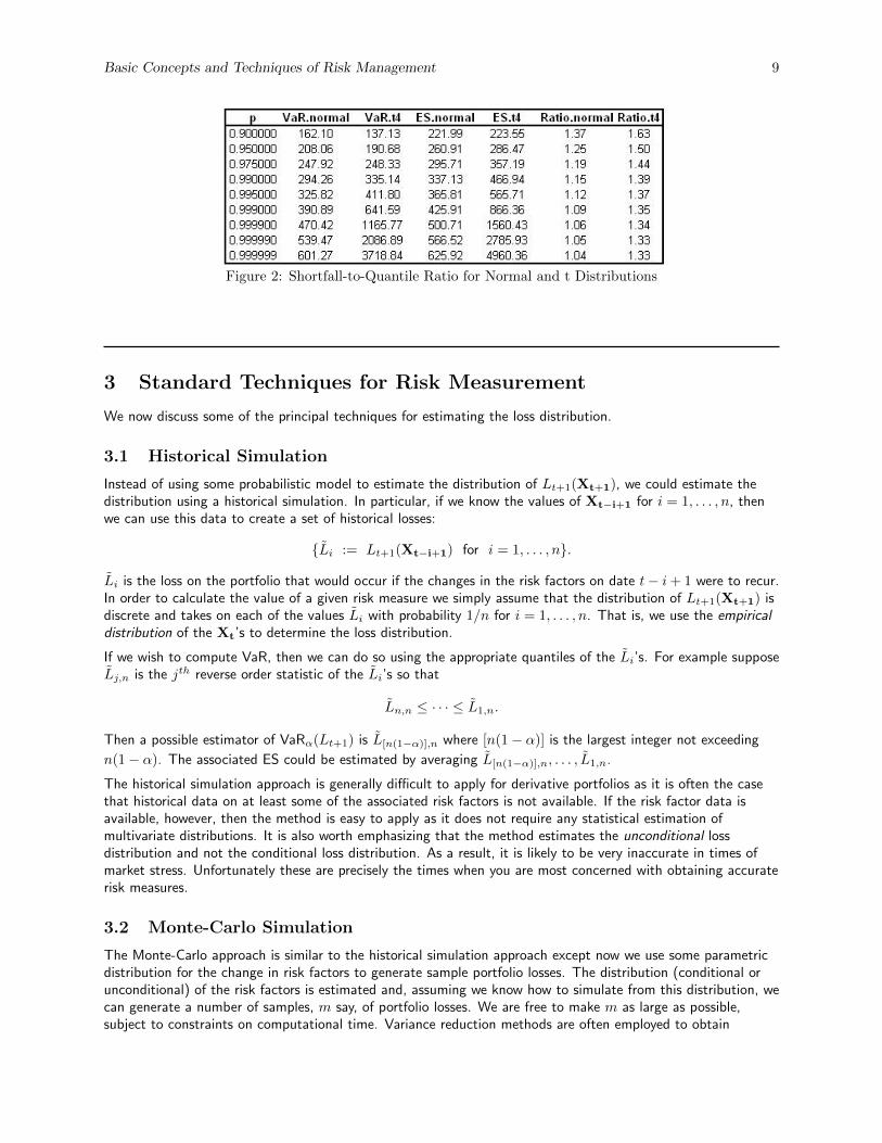
Basic Concepts and Techniques of Risk Management 9
Figure 2: Shortfall-to-Quantile Ratio for Normal and t Distributions
3 Standard Techniques for Risk Measurement
We now discuss some of the principal techniques for estimating the loss distribution.
3.1 Historical Simulation
Instead of using some probabilistic model to estimate the distribution of Lt+1(Xt+1), we could estimate thedistribution using a historical simulation. In particular, if we know the values of Xt−i+1 for i = 1, . . . , n, thenwe can use this data to create a set of historical losses:
{L̃i := Lt+1(Xt−i+1) for i = 1, . . . , n}.
L̃i is the loss on the portfolio that would occur if the changes in the risk factors on date t− i+ 1 were to recur.In order to calculate the value of a given risk measure we simply assume that the distribution of Lt+1(Xt+1) isdiscrete and takes on each of the values L̃i with probability 1/n for i = 1, . . . , n. That is, we use the empiricaldistribution of the Xt’s to determine the loss distribution.
If we wish to compute VaR, then we can do so using the appropriate quantiles of the L̃i’s. For example supposeL̃j,n is the jth reverse order statistic of the L̃i’s so that
L̃n,n ≤ · · · ≤ L̃1,n.
Then a possible estimator of VaRα(Lt+1) is L̃[n(1−α)],n where [n(1− α)] is the largest integer not exceeding
n(1− α). The associated ES could be estimated by averaging L̃[n(1−α)],n, . . . , L̃1,n.
The historical simulation approach is generally difficult to apply for derivative portfolios as it is often the casethat historical data on at least some of the associated risk factors is not available. If the risk factor data isavailable, however, then the method is easy to apply as it does not require any statistical estimation ofmultivariate distributions. It is also worth emphasizing that the method estimates the unconditional lossdistribution and not the conditional loss distribution. As a result, it is likely to be very inaccurate in times ofmarket stress. Unfortunately these are precisely the times when you are most concerned with obtaining accuraterisk measures.
3.2 Monte-Carlo Simulation
The Monte-Carlo approach is similar to the historical simulation approach except now we use some parametricdistribution for the change in risk factors to generate sample portfolio losses. The distribution (conditional orunconditional) of the risk factors is estimated and, assuming we know how to simulate from this distribution, wecan generate a number of samples, m say, of portfolio losses. We are free to make m as large as possible,subject to constraints on computational time. Variance reduction methods are often employed to obtain

Basic Concepts and Techniques of Risk Management 10
improved estimates of the required risk measures. While Monte-Carlo is an excellent tool, it is only as good asthe model used to generate the data: if the distribution of Xt+1 that is used to generate the samples is poor,then the Monte-Carlo samples will be of little value.
3.3 Variance-Covariance Approximations
In the variance-covariance approach we assume that Xt+1 has a multivariate normal distribution so that
Xt+1 ∼ MVN (µ,Σ) .
We also assume that the linear approximation in (3) is sufficiently accurate. Writing
L̂t+1(Xt+1) = −(ct + bt>Xt+1) for a constant scalar, ct, and constant vector, bt, we therefore obtain that
L̂t+1(Xt+1) ∼ N(−ct − bt
>µ, bt>Σbt
).
We can now use our knowledge of the normal distribution to calculate any risk measures of interest. Note thatthis technique can be either conditional or unconditional, depending on how µ and Σ are estimated.
The strength of this approach is that it provides a straightforward analytically tractable method of determiningthe loss distribution. It has several weaknesses, however. Risk factor distributions are often9 fat- or heavy-tailedbut the normal distribution is light-tailed. As a result, we are likely to underestimate the frequency of extrememovements which in turn can lead to seriously underestimating the risk in the portfolio. This problem isgenerally easy to overcome as there are other multivariate distributions that are also closed under linearoperations. In particular, if we assume that Xt+1 has a multivariate t distribution so that
Xt+1 ∼ t (ν, µ,Σ)
then we obtainL̂t+1(Xt+1) ∼ t
(ν,−ct − bt
>µ, bt>Σbt
).
where ν is the degrees-of-freedom of the t-distribution. A more serious problem with this approach is theassumption that the linear approximation will work well. This is generally not true for portfolios of derivativesecurities or other portfolios where the portfolio value is a non-linear function of the risk-factors. It is alsoproblematic when the time horizon ∆ is large. We can also overcome this problem to some extent by usingquadratic approximations to Lt+1 instead of linear approximations and then using Monte-Carlo to estimate therisk measures of interest.
3.4 Evaluating the Techniques for Risk Measurement
An important task of any risk manger is to constantly evaluate the risk measures that are being reported. Forexample, if the daily 95% VaR is reported then we should see the daily losses exceeding the reported VaRapproximately 95% of the time. Indeed, suppose the reported VaR numbers are calculated correctly and let Yibe the indicator function denoting whether or not the portfolio loss in period i exceeds VaRi, the correspondingVaR for that period. That is
Yi =
{1, Li ≥ VaRi;0, otherwise.
If we assume the Yi’s are IID, then∑ni=1 Yi should be Bin(n, .05). We can use standard statistical tests to see if
this is indeed the case. Similar tests can be constructed for ES and other risk measures.
More generally, it is important to check that the true reported portfolio losses are what you would expect giventhe composition of the portfolio and the realized change in the risk factors over the previous period. Forexample, if you know the delta and vega of your portfolio at time ti−1 and you observe the change in theunderlying and volatility factors between ti−1 and ti, then the actual realized gains or losses should beconsistent with the delta and vega numbers. If they are not, then further investigation is required. It may be
9We will define light- and heavy-tailed distributions formally when we discuss multivariate distributions.
Basic Concepts and Techniques of Risk Management 11
that (i) the moves required second order terms such as gamma, vanna or volga or (ii) other risk factorsinfluencing the portfolio value also changed or (iii) the risk factor moves were very large and cannot be capturedby any Taylor series approximation – see the related discussion below (8). Of course one final possibility is thatthere’s a bug in the risk management system!
4 Other Considerations
In this section we briefly describe some other issues that frequently arise in practice. We will return to some ofthese issues at various points throughout the course.
4.1 Risk-Neutral and Data-Generating Measures
It is worth emphasizing that in risk management, we generally want to generate loss samples using the trueprobability measure, P . This is in contrast to security pricing where we use a risk-neutral or equivalentmartingale measure, Q. Sometimes, however, we need to use both probability measures. Imagine for example, aportfolio of complex derivatives that we can only price using Monte-Carlo. In order to estimate the lossdistribution, we would then (i) generate samples of the change in risk factors using P and (ii) for each suchsample, compute the resulting value of the portfolio by running a Monte-Carlo using Q.
4.2 Data Risk
When using historical data to either estimate probability distributions or run a historical simulation analysis, forexample, it is important to realize that the data may be biased in several ways. For example, survivorship bias isa common problem: the stocks that exist today are more likely to have done well than the stocks that no longerexist. So when we run a historical simulation to evaluate the risk of a long stock portfolio, say, we are implicitlyomitting the worst returns from our analysis and therefore introducing a bias into our estimates of the variousrisk measures. We can get around this problem if we can somehow include the returns of stocks that no longerexist in our analysis. We also need to be mindful of biases that arise due to data mining or data snoopingwhereby people trawl through data-sets looking for spurious data patterns to justify some investment strategy.The newsletter scam is a classic example of what can go wrong! In some cases, selection bias may be presentinadvertently. Regardless, one should always be alert to the possibility of these biases.
4.3 Multi-Period Risk Measures and Scaling
It is often necessary to report risk measures with a particular investment horizon in mind. For example, manyhedge funds are required by investors to report their 10-day 95% VaR and the question arises as to how thisshould be calculated. They could of course try to estimate the 10-day VaR directly. However, as hedge fundstypically calculate a 1-day 95% VaR anyway, it would be convenient if they could somehow scale the 1-day VaRin order to estimate the 10-day VaR. Before considering this problem, it is worth emphasizing one of the implicitassumptions that we make when calculating our risk measures:
The Constant Portfolio Composition Assumption: The risk measures are calculated by assuming thatthe portfolio composition does not change over the horizon [t∆, (t+ 1)∆].
Indeed regulatory requirements typically require that VaR be calculated under this assumption. While this isusually ok for small values of ∆, e.g. 1 day, it makes little sense for larger values of ∆, e.g. 10 days, duringwhich the portfolio composition is very likely to change. In fact in some circumstance the portfolio compositionmust change. Consider an options portfolio where some of the options are due to expire before the interval, ∆,elapses. If the options are not cash settled, then any in-the-money options will be exercised resultingautomatically in new positions in the underlying securities. Regardless of how the options settle, the returns onthe portfolio around expiration will definitely not be IID. It can therefore be very problematic scaling a 1-day

Basic Concepts and Techniques of Risk Management 12
VaR into a 10-day VaR in these circumstances. More generally, it may not even make sense to consider a 10-dayVaR when you know the portfolio composition is likely to change dramatically.
When portfolio returns are IID and factor changes are normally distributed then a square-root scaling rule can bejustified. In this case, for example, we could take the 10-day VaR equal to
√10 times the 1-day VaR. This
follows from Example 4 with µ = 0 and the assumption of continuously compounded returns. But this kind ofscaling can lead to very misleading results when portfolio returns are not IID normal, even when the portfoliocomposition does not change.
4.4 Model Risk
Model risk can arise when calculating risk measures or estimating loss distributions. For example, if we areconsidering a portfolio of European options then there should be no problem in using the Black-Scholes formulato price these options as long as we use appropriate volatility risk factors with appropriate distributions. Butsuppose instead that the portfolio contains barrier options and that we use the corresponding Black-Scholesmodel for pricing these options. Then we are likely to run into several difficulties as the model is notoriouslybad. It is possible, for example, that reported risk measures such as delta or vega will have the wrong sign!Moreover, the range of possible barrier option prices is limited by the assumption of constant volatility. A moresophisticated model would allow for a greater range of prices, and therefore losses. A more obvious example ofmodel risk is using a light-tailed distribution to model risk factors when in fact a heavy-tailed distribution shouldbe used.
4.5 Data Aggregation
A particularly important topic is the issue of data aggregation. In particular, how do we aggregate risk measuresfrom several trading desks or several units within a firm into one single aggregate measure of risk? This issuearises when a firm is attempting to understand its overall risk profile and determining its capital adequacyrequirements as mandated by regulations. One solution to this problem is to use sub-additive risk measures thatcan be added together to give a more conservative measure of aggregate risk. We will return to this topic whenwe discuss coherent measures of risk.
Another solution is to simply ignore the risk measures from the individual units or desks. Instead we could try todirectly calculate a firm-wide risk number. This might be achieved by specifying scenarios that encompass thefull range of risk-factors to which the firm is exposed or using the variance-covariance approach with many riskfactors. The resulting mean vector, µ, and variance-covariance matrix, Σ, may be very high-dimensional,however. For a small horizon, ∆, it is generally ok to set µ = 0 but it will often be very difficult to estimate Σdue to its high dimensionality. In that case factor models and other techniques can often be used to constructmore reliable estimates of Σ.
4.6 Liquidity Risk
Liquidity risk is a very important source of risk particularly if we need to unwind a portfolio. We may know the“fair” market price of the portfolio in a given scenario but will we be able to transact or unwind at that priceshould the scenario occur? If we expect bid-ask spreads to be tight in that scenario then it is indeed reasonableto assume that we can unwind at approximately the “fair” price. But if the scenario is an extreme scenario thenit’s possible the bid-ask spreads will have widened substantially so that transacting at the fair price will beimpossible. This situation can be exacerbated if many firms hold similar portfolios and are all “rushing for theexits“ at the same time. In that event enormous losses can be incurred in the act of unwinding the portfolio.This is the “crowded trade” phenomenon and it was a source of many of the extreme losses that occurredduring the 2008 crisis.
Liquidity risk is difficult to model but does need to be accounted for if many firms also hold a similar positionand we expect that we may need to unwind our position should the scenario occur. One way to account for thisis to model the bid-ask spread in the various scenarios and use these to compute an “unwind” P&L in additionto the market P&L (which does not assume unwinding is necessary and will take the fair price to be themid-point of the bid-ask spread.)
Basic Concepts and Techniques of Risk Management 13
4.7 P&L Attribution
Risk management is typically about understanding the risks in a portfolio in anticipation of future changes in theunderlying risk factors. In contrast, P&L attribution is a backward-looking process where the goal is tounderstand what risk factor (changes) have contributed to the P&L that has been realized between times t andt+ 1. There are at least a couple of approaches to solving this problem. Consider, for example, a Europeanoption on a stock or index:
1. One approach is based on local approximations via Taylor’s Theorem. Let Returnt,t+1 and ∆σt,t+1 denotethe changes in risk-factors (in this example the underlying return and change in implied volatility) between
times t and t+ 1. We can then use (8) to obtain a predicted P&L, P&Lpredt,t+1, as a function of the Greeksat time t and the changes in risk-factors:
P&Lpredt,t+1 ≈ ESPt × Returnt,t+1 + $ Gammat × Return2t,t+1 + vegat∆σt,t+1. (14)
Note that P&Lpredt,t+1 is the P&L we would predict for the period [t, t+ 1] standing at time t if we knewwhat the changes in risk factors were going to be over that period. Once time t+ 1 arrives we can observethe realized P&L, P&Lrealt,t+1. We can then write this as
P&Lrealt,t+1 = P&Lpredt,t+1 + εt,t+1 (15)
where εt,t+1 is defined to be whatever value makes (15) true. Ideally εt,t+1 would be very small so thatthe predicted P&L given by (14) accounts for almost all of the realized P&L. Note that we can then use(14) to attribute the P&L to delta (ESP), gamma and vega respectively. If εt,t+1 is large, however, thenthe attribution has performed poorly. In that case we would need to include other risk factors, e.g. thetafor the (deterministic) passage of time or a dividend factor to account for changes in expected dividends,or else include other second-order sensitivities such as volga, vanna etc. Even then, however, becauseapproximations like (14) are only valid for “small” changes in the risk factors, it is quite possible that thisapproach will fail in extremely volatile markets such as those encountered at the height of the financialcrisis in 2008.
2. An alternative is to use a more global approach that is not based on the (mathematical) derivatives, i.e.the Greeks, that are required by a Taylor series approximation. Such an approach is coarser than the localapproach but it will work in extremely volatile markets as long as all important risk factors are included inthe analysis.