ieee transactions on visualization and computer graphics, vol. 11

Creating and Simulating Skeletal Musclefrom the Visible Human Data Set

Joseph Teran, Eftychios Sifakis, Silvia S. Blemker,

Victor Ng-Thow-Hing, Cynthia Lau, and Ronald Fedkiw

Abstract—Simulation of the musculoskeletal system has important applications in biomechanics, biomedical engineering, surgery

simulation, and computer graphics. The accuracy of the muscle, bone, and tendon geometry as well as the accuracy of muscle and

tendon dynamic deformation are of paramount importance in all these applications. We present a framework for extracting and

simulating high resolution musculoskeletal geometry from the segmented visible human data set. We simulate 30 contact/collision

coupled muscles in the upper limb and describe a computationally tractable implementation using an embedded mesh framework.

Muscle geometry is embedded in a nonmanifold, connectivity preserving simulation mesh molded out of a lower resolution BCC lattice

containing identical, well-shaped elements, leading to a relaxed time step restriction for stability and, thus, reduced computational cost.

The muscles are endowed with a transversely isotropic, quasi-incompressible constitutive model that incorporates muscle fiber fields

as well as passive and active components. The simulation takes advantage of a new robust finite element technique that handles both

degenerate and inverted tetrahedra.

Index Terms—Finite volume methods, constructive solid geometry, physically-based modeling.

�

1 INTRODUCTION

SIMULATION of anatomically realistic musculature andflesh is critical for many disciplines, including biome-

chanics, biomedical engineering, and computer graphics,where it is becoming an increasingly important component ofany virtual character. Animated characters must have skinthat deforms in a visually realistic manner. However, thecomplexity of the interaction of muscles, tendons, fat, andother soft tissueswith the enveloping skin andour familiaritywith this type ofmotionmake these animations difficult if notimpossible to create procedurally. In biomechanics andbiomedical engineering, accurate descriptions of musclegeometry are needed to characterize muscle function.Knowledge of such quantities asmuscle length, line of action,and moment arm is essential for analyzing a muscle’s abilityto create forces, produce joint moments, and actuate motion[32]. For example, many studies use knowledge of musclelengths [1] and moment arms [2] to analyze muscle functionfor improving diagnosis and treatment of people withmovement disabilities.

In order to create realistic flesh deformation for

computer graphics characters, anatomy-based modeling

techniques of varying resolutions are typically applied.

These models are generally composed of an underlyingskeleton whose motion is prescribed kinematically (frommotion capture or traditional animation) and a model thattransmits motion of the underlying skeleton to tissuedeformation. The model for this interaction can havevarying levels of detail. For example, [25] maps jointconfigurations to skin deformers that procedurally warpthe surface of the character. The work in [43] and [35] usedanatomically-based models of muscles, tendons, and fattytissue to deform an outer skin layer. The deformation of themuscle and tendon primitives was based on musclecharacteristics such as incompressibility, but dynamiceffects were not included. An obvious improvement to thisapproach is to include dynamic effects based on musclemechanics, as in [9], [22], [37], which incorporatedtheoretical muscle dynamic models (e.g., the relationbetween force, length, and velocity in muscle) using theequations of solid mechanics to simulate muscle contrac-tion. However, in [9], [37], computational complexityrestricted the application of their techniques to only a fewmuscles at a time. Hirota et al. [22] simulated more tissuesin the knee, but the dynamics were simulated quasistati-cally, ignoring the visually appealing effects of ballisticmotion and inertia.

Musculoskeletal simulations inbiomechanics typically fallinto two categories: simulations of simple models for manymuscles composing a large region of the body (e.g., the upperlimb or lower extremity) or highly detailed muscle modelsthat can only be simulated a fewmuscles at a time. Commonmuscle models compute accurate muscle moment arms andmuscle/tendon lengths, but only resolve the average muscleline of action [13], [18].However, it is difficult to represent thepath of a muscle with complex geometry because it requiresknowledge of how, as joints move, themuscle changes shapeand interacts with underlying muscles, bones, and other

IEEE TRANSACTIONS ON VISUALIZATION AND COMPUTER GRAPHICS, VOL. 11, NO. 3, MAY/JUNE 2005 317

. J. Teran, E. Sifakis, C. Lau, and R. Fedkiw are with the Computer ScienceDepartment, Stanford University, Gate Computer Science Bldg., Stanford,CA 94305-9020.E-mail: {jteran, sifakis, cindabin}@stanford.edu, [email protected].

. S.S. Blemker is with the Bioengineering Department, Stanford University,James H. Clark Center, Room S-355, 318 Campus Dr., Stanford, CA94305-5450. E-mail: [email protected].

. V. Ng-Thow-Hing is with the Honda Research Institute USA, 800California St., Suite 300, Mountain View, CA 94041.E-mail: [email protected].

Manuscript received 13 Apr. 2004; revised 12 Oct. 2004; accepted 2 Nov.2004; published online 10 Mar. 2005.For information on obtaining reprints of this article, please send e-mail to:[email protected], and reference IEEECS Log Number TVCG-0037-0404.

1077-2626/05/$20.00 � 2005 IEEE Published by the IEEE Computer Society

structures. These simplified models typically require theconstruction of elaborate “wrapping” surfaces and “viapoints” to resolve contact with other muscles and bones incompensation for simplifying muscles as piecewise linearbands. These simplified models of contact are difficult toconstruct robustly as they require an a priori knowledgeof the contact environment that is not always available.More detailed muscle models do not suffer from thesedifficulties, but are burdened by computational complex-ity. Typical examples are [44] and [19], which used modernnonlinear solid mechanics to recreate the stress anddeformation, although only a few muscles with simplifiedgeometry were considered and the simulations were carriedout quasistatically to avoid the stringent time step restric-tions characteristic of explicit schemes.

We present a framework that can be used to createhighly realistic virtual characters while still allowing forbiomechanically accurate simulation of large musclegroups. We present a pipeline for creating musculoskeletalmodels from the segmented visible human data set thatallows for the creation of highly detailed models of muscle,tendon and bone. We demonstrate this by creating amusculoskeletal model of the upper limb. Then, we embedeach high resolution muscle geometry in a nonmanifold,uniform simulation mesh. The embedding mesh is com-prised of identical, well-conditioned elements, thus sig-nificantly relaxing the time step restriction, allowing us toavoid quasistatic simulation. Since the elements in eachmesh are identical, we only need to store the materialcoordinates of a single undeformed tetrahedron per muscleas opposed to storing material information for everyelement in the mesh. Contact is treated directly based onmuscle geometry as opposed to procedurally created, error-prone wrapping surfaces. The inclusion of inertia forceswhile performing the simulations in [37] illustrated theimportance of the tendonous connective tissue networksthat wrap muscle groups. In response to this phenomenon,we incorporate the effects of these tissues in a contact/collision algorithm that works between the high-resolutiongeometry and the low-resolution simulation mesh.

2 RELATED WORK

Terzopoulos et al. [39], [38] simulated deformable materials,including the effects of elasticity, viscoelasticity, plasticity,and fracture. Although they mentioned that either finitedifferences or the FEM could be used, they seemed to prefera finite difference discretization. Subsequently, [20] advo-cated the FEM for simulating a human hand grasping a balland, since then, a number of authors have used the FEM tosimulate volumetric deformable materials.

Chen and Zelzer [9] used the FEM, brick elements, andthe constitutive model of [45] to simulate a few muscles,including a human bicep. Due to computational limitationsat the time, very few elements were used in the simulation.Wilhems and Van Gelder [43] built an entire model of amonkey using deformed cylinders as muscle models. Theirmuscles were not simulated, but, instead, deformedpassively as the result of joint motions. Scheepers et al.[35] carried out similar work developing a number ofdifferent muscle models that change shape based on the

positions of the joints. They emphasized that a plausibletendon model was needed to produce the characteristicbulging that results from muscle contraction. A recent trendis to use the FEM to simulate muscle data from the visiblehuman data set, see, e.g., [46], [22], [14], [15].

In order to increase the computational efficiency, anumber of authors have been investigating adaptivesimulation. Debunne et al. [10] used a finite differencemethod with an octree for adaptive resolution. This waslater improved in [12] using a weighted finite differenceintegration technique (which they mistakenly referred to as“finite volume”) to approximate the Laplacian and thegradient of the divergence operators. Debunne et al. [11]used FEM with a multiresolution hierarchy of tetrahedralmeshes and Grinspun et al. [21] refined basis functionsinstead of elements.

3 MODEL CREATION

Geometrically accurate musculoskeletal models are desiredin graphics, biomechanics, and biomedical engineering.However, the intricacy of the human anatomy makes itdifficult to procedurally create models of the musculatureand skeleton. As a consequence, researchers have turned tovolume data from actual human subjects as a source forgeometry. One such source is the visible human data set,which consists of high-resolution images of millimeter-spaced cross sections of an adult male [41]. We use asegmented version of this data to create the muscle, tendon,and skeleton geometry for our simulations. Using thesegmented anatomy information, we first create level setrepresentations of each tissue intended for simulation.Unfortunately, the segmented data often contains imperfec-tions or is unfit for creating a reasonable simulation mesh.We repair each tissue using simple level set smoothingtechniques (see, e.g., [31]) and/or CSG operations. Atetrahedralized volume is then produced for each muscle(including tendon) and a triangulated surface is producedfor each bone (see Fig. 1). Both of these are created using theimplicit surface meshing framework of [27], [7].

Once the muscle, tendon, and bone geometries have beencreated, we encode necessary additional information intoeach muscle representation including material heterogene-ity (tendon is stiffer than muscle and does not undergoactive contraction) as well as spatially varying muscle fiberdirections. Additionally, the kinematic structure of theunderlying skeleton must be created to drive skeletalmotion. Finally, boundary conditions are specified to attachmuscle and tendon to bone.

3.1 Level Set Extraction

Due to the large amount of noise and occasional inaccura-cies present in the segmented data, creating our modelbegins with examining and fixing such problems. We relyon a dual explicit/implicit representation of the musclegeometry to facilitate the repair process. We first create alevel set representation of each tissue we wish to simulateusing the visible human data. This data consists of gray-scale images of 1.0 mm axial slices of the entire body withindividual tissues and bones assigned different values.Information of this type naturally converts to Heaviside

318 IEEE TRANSACTIONS ON VISUALIZATION AND COMPUTER GRAPHICS, VOL. 11, NO. 3, MAY/JUNE 2005

descriptions of each individual tissue. The meshing algo-rithm we use to create the explicit geometric representations(tetrahedralized volume or triangulated surface) as well asthe level set procedures we use to smooth noisy datarequire a signed distance function which we generate usingthe fast marching method [40], [36].

After the level sets are generated, slice-by-slice contoursculpting is used to repair problem regions. First, each sliceof a generated level set is viewed graphically to check forand eliminate errors that would otherwise interfere witheither the anatomical accuracy of our model or thealgorithm for the subsequent meshing process. We thenuse basic level set smoothing techniques such as motion bymean curvature (see, e.g., [31]) to eliminate any furthernoise automatically.

3.2 Meshing Bone and Muscle

Once the level sets are free of the inaccuracies and noisepresent in the original data, we use them to construct atriangulated surface representation of each bone and atetrahedralized volume representation of each muscle [27],[7]. The tetrahedral mesh generation algorithm begins bypartitioning all of space with a body-centered cubic (BCC)tetrahedral lattice and extracting the subset of the tetra-hedra that intersect with the object volume defined by thelevel set. Then, a red green mesh subdivision algorithm isused to refine the initial mesh to an appropriate level ofdetail, using both curvature and surface information asrefinement criteria. Extra care is taken with elements nearthe boundary in order to obtain a well-conditioned

simulation mesh. Finally, using either a mass spring orfinite element model, the boundary nodes of the mesh arecompressed toward the zero isocontour of the signeddistance function. For the triangulated surfaces used forthe rigid bodies, this procedure is carried out with thesurface of the BCC lattice.

3.3 Tendon and Bone Attachment Designation

A major flaw in the segmented data set is that a largeamount of tendon tissue is absent. For example, thesegmented biceps data lacks any information about thedistal tendon and its proximal tendons are underresolved.In order to add missing tendon tissue to each muscle mesh,we make use of both explicit and implicit representations ofeach muscle. While explicit representations allow for moreefficient and accurate graphical rendering of objects,implicit representations are advantageous for Booleanoperations. Our method for regenerating missing tendontissue for a given muscle mesh makes use of simple CSGmethods on graphically positioned tendon primitives. Aftera set of tendon primitives is positioned in relation to amuscle mesh where its missing tendon tissue should be, theunion of the tendon primitives and the muscle mesh iscalculated and converted into a new level set (see Fig. 2).This new level set then undergoes another iteration of theediting, smoothing, and meshing processes describedabove. Due to the efficiency of the level set creation andtetrahedral meshing algorithms, the cost of this seconditeration is reasonable. The result of this step is an improvedtetrahedralized volume representation for each muscle that

TERAN ET AL.: CREATING AND SIMULATING SKELETAL MUSCLE FROM THE VISIBLE HUMAN DATA SET 319

Fig. 2. Musculotendon mesh creation using CSG to repair errors in the bicepts tendons. Heterogeneous tendon tetrahedra are selected using the

Fig. 1. Musculoskeletal model created from the visible human data set. Tendons are shown in pink. There are about 10 million tetrahedra in the

approximately 30 muscles depicted.

includes both the muscle tissue and all of its associated

tendon tissue.To improve the accuracy of our model during simula-

tion, it is necessary not only to include tendons in the

tetrahedronmeshes, but also to differentiate betweenmuscle

and tendon tissue as well as to define muscle-bone attach-

ment regions. Therefore, we define subregions within each

muscle mesh to represent muscle tissue, tendon tissue, and

bone attachment regions. Tetrahedra designated as muscle

are influenced by muscle activations, whereas those desig-

nated as tendon remain passive during simulation. Further-

more, tendon tissue is an order of magnitude stiffer than

muscle tissue. Tendon often extends into the belly of certain

muscles, forming an internal layer of passive tissue to which

the activemuscle fibers attach. This layer of connective tissue

is known as an aponeurosis and can play a large role inmany

muscle functions [33], [16]. We take extra care to model this

layer when selecting the regions of the muscle/tendon

geometry to designate as tendon. Additionally, we rigidly

attach tetrahedrons in the origin and insertion regions of each

musclemesh to their corresponding bones. Tetrahedrons that

are designated as attached to bone are used to set Dirichlet

boundary conditions during simulations.Our method for defining the subregions described above

involves graphically selecting portions of the mesh to be

tendon or bone attachment tetrahedra, leaving the remain-

ing tetrahedra designated as muscle. In general, we use

closed triangulated surfaces to select groups of tetrahedra

making use of anatomy texts for anatomical accuracy.

However, a good initial guess can be calculated by simply

using a proximity threshold of the tetrahedra to a particular

bone. We correct this guess by growing regions initially

selected based on mesh connectivity as well as by graphical

selection. See Fig. 3.

3.4 B-Spline Fiber Representation

Muscle tissue fiber arrangements vary in complexity from

being relatively parallel and uniform to exhibiting several

distinct regions of fiber directions. We use B-spline solids to

assign fiber directions to individual tetrahedrons of our

muscle simulation meshes, querying the B-spline solid’s

local fiber direction at a spatial point corresponding to the

centroid of a tetrahedron as in [29].B-spline solids have a volumetric domain and a compact

representation of control points, qijk, weighted by B-spline

basis functions BuðuÞ; BvðvÞ; BwðwÞ:

Fðu; v; wÞ ¼Xi

Xj

Xk

Bui ðuÞBv

jðvÞBwk ðwÞqijk;

whereF is a volumetric vector functionmapping thematerialcoordinates ðu; v; wÞ to their corresponding spatial coordi-nates. Taking the partial derivatives of Fwith respect to oneof the three material coordinates @F=@u, @F=@v, @F=@wproduces an implicit fiber field defined in the materialcoordinate direction. In [29], one of these directions alwayscoincidedwith the local tangent of themuscle fiber located atthe spatial position corresponding to the material coordi-nates. The inverse problem of finding the material coordi-nates for a given spatial point can be solved using numericalroot-finding techniques to create a fiber query function

XðxÞ ¼ @FðF�1ðxÞÞ=@m@FðF�1ðxÞÞ=@m

�� ;with m ¼ fu; v; wg depending on the parameter chosen andthe fiber directions normalized. The functionX describes anoperation that first inversely maps the spatial points back totheir corresponding material coordinates ðu; v; wÞ and thencomputes the normalized fiber direction at that point.

We created these B-spline solids based on anatomy texts,however, working with anatomy experts as in [29] or usingfiber information from scanning technologies would im-prove accuracy. Additionally, using a fiber primitivetemplate as was done in [3] would also improve accuracyand simplify the process.

3.5 Skeletal Motion

Bones are naturally articulated by ligaments and other softtissues that surround them. However, we consider theinverse problem: a kinematic skeleton that drives themotion and contraction of the muscles and tendonsattached to it. The joint spaces used to create a realistickinematic structure involve intricate couplings of revoluteand prismatic components resulting from the geometriccomplexity and redundancy of the muscles, tendons, andligaments that articulate the bones. Fortunately, there ismuch existing literature dedicated to the joint structures inthe human body. We turned to the results of [17] to createthe kinematic structure of the upper limb. In [17], the visiblemale was used to create a skeleton model of the rightshoulder, elbow, and wrist. Anatomical landmarks werethen used to identify joint centers and to set up localcoordinate frames for each of the bones. State of the art jointmodels with 13 overall degrees of freedom were used todescribe the relative motion of the sternum, clavicle,


Fig. 3. Bone attachment process for the subscapularis and scapula. Constrained tetrahedra are shown in yellow, tendon tetrahedra are shown in

pink. Bone attachment regions are determined by proximity and from anatomy texts.

scapula, humerus, radius, and ulna. Using the same virtual

anatomy, we were able to directly incorporate their results.Additional work was done in [18] to create a muscle

model in the upper limb based on the Obstacle Set method

for computing musculo-tendon paths, see Fig. 4 (left). This

model for muscle length and moment arm computation

assumes constant cross-sectional stress and simplifies the

muscles to average lines of action. Basic geometric

primitives like cylinders and spheres are used as collision

objects to compute the paths of muscles as they collide with

bones and other tissues. With this infrastructure in place,

we use an inverse dynamics analysis with the results of [37]

to compute activations for the muscles in the right upper

limb. These techniques work with both motion capture and

traditional animation.

4 FINITE VOLUME METHOD

4.1 Force Computation

The Finite Volume Method provides a simple and

geometrically intuitive way of integrating the equations

of motion with an interpretation that rivals the simplicity

of mass-spring systems. However, unlike masses and

springs, an arbitrary constitutive model can be incorpo-

rated into the FVM.In the deformed configuration, consider dividing up the

continuum into a number of discrete regions, each

surrounding a particular node. Fig. 5 depicts two nodes,

each surrounded by a region. Suppose that we wish to

determine the force on the node xi surrounded by the

shaded region �. Ignoring body forces for brevity, the force

can be calculated as

f i ¼D

Dt

Z�

�vdx ¼I@�

tdS ¼I@�

��ndS;

where � is the density, v is the velocity, and t is the surface

traction on @�. The last equality comes from the definition of

theCauchy stress��n ¼ t. Evaluationof theboundary integral

requires integrating over the two segments interior to each

incident triangle. Since �� is constant in each triangle and the

integral of the local unit normal over any closed region is

identically zero (from the divergence theorem), we have

I@�1

��ndS þI@�2

��ndS þI@T1

��ndS þI@T2

��ndS ¼ 0;

where @T1 and @T2 are depicted in Fig. 6 (left).More importantly, we have

I@�1

��ndS þI@�2

��ndS ¼ �I@T1

��ndS �I@T2

��ndS;

indicating that the integral of ��n over @�1 and @�2 can be

replaced by the integral of ��n over @T1 and @T2. That is,

for each triangle, we can integrate over the portions of its

edges incident to xi instead of the two interior edges @�1

and @�2. Moreover, even if @�1 and @�2 are replaced by an

arbitrary path inside the triangle, we can replace the

integral over this region with the integral over @T1 and

@T2. We choose an arbitrary path inside the triangles that

connects the midpoints of the two edges incident on xi, as

shown in Fig. 6 (right). Then, the surface integrals are

simply equal to ��n1e1=2 and ��n2e2=2, where e1 and e2are the edge lengths of the triangles. Thus, the force on node

xi is updated via

f iþ ¼ � 1

2�� e1n1 þ e2n2ð Þ:


Fig. 4. The leftmost figure shows the piecewise linear muscle models with wrapping surfaces to model muscle contact in inverse dynamics

calculations. Larger muscles have multiple contractile regions with individual activations and these must be embedded in the tetrahedron meshes for

simulation (rightmost figures).

Fig. 5. FVM integration regions. Fig. 6. Integration over a triangle.

In three spatial dimensions, given an arbitrary stress ��,regardless of the method in which it was obtained, weobtain the FVM force on the nodes in the following fashion:Loop through each tetrahedron, interpreting �� as theoutward pushing “ multidimensional force.” For each face,multiply by the outward unit normal to calculate thetraction on that face. Then, multiply by the area to find theforce on that face and simply redistribute one-third of thatforce to each of the incident nodes. Thus, each tetrahedronwill have three faces that contribute to the force on each ofits nodes, e.g., the force on node xi is updated via

f iþ ¼ � 1

3�� a1n1 þ a2n2 þ a3n3ð Þ:

Note that the cross product of two edges is twice the area ofa face times the normal, so we can simply add one-sixth of�� times the cross product to each of the three nodes.

4.2 Piola-Kirchhoff Stress

A deformable object is characterized by a time dependentmap � from undeformed material coordinates X todeformed spatial coordinates x. We use a tetrahedron meshand assume that the deformation is piecewise linear, whichimplies �ðXÞ ¼ FXþ b in each tetrahedron. For simplicity,consider two spatial dimensions where each element is atriangle. Fig. 7 depicts amapping� froma triangle inmaterialcoordinates to the resulting triangle in spatial coordinates.We define edge vectors for each triangle as dm1

¼ X1 �X0,dm2

¼ X2 �X0, ds1 ¼ x1 � x0, and ds2 ¼ x2 � x0. Note thatds1 ¼ FX1 þ bð Þ � FX0 þ bð Þ ¼ Fdm1

and, likewise, ds2 ¼Fdm2

so that F maps the edges of the triangle in materialcoordinates to the edges of the triangle in spatial coordinates.Thus, ifweconstruct2� 2matricesDmwith columnsdm1

anddm2

, and Ds with columns ds1 and ds2 , then Ds ¼ FDm orF ¼ DsD

�1m . The matrix F is known as the deformation

gradient and conveys all the necessary information todetermine the material response to deformation since thetranslational component of � does not induce any stress. Inthree spatial dimensions,Dm andDs are 3� 3matrices withcolumns equal to the edge vectors of the tetrahedra. Note thatD�1

m can be be precomputed and stored for efficiency.Often, application of a constitutive model will result in a

second Piola-Kirchoff stress, S, which can be converted to aCauchy stress via �� ¼ J�1FSFT , where J ¼ detðFÞ. Usingthis equality and the identity an ¼ JF�TAN, we can write

f iþ ¼ � 1

3P A1N1 þA2N2 þA3N3ð Þ;

where P ¼ FS is the first Piola-Kirchhoff stress tensor, theAi are the areas of the undeformed tetrahedron facesincident to Xi, and the Ni are the normals to thoseundeformed faces.

Since the Ai and Ni do not change during thecomputation, we can precompute and store these quantities.Then, the force contribution to each node can be computedas gi ¼ Pbi, where the bi are precomputed and the force oneach node is updated with f iþ ¼ gi. Moreover, we can savenine multiplications by computing g0 ¼ �ðg1 þ g2 þ g3Þinstead of g0 ¼ Pb0. We can compactly express thecomputation of the other gi as G ¼ PBm, where G ¼ðg1;g2;g3Þ and Bm ¼ ðb1;b2;b3Þ. Thus, given an arbitrarystress S in a tetrahedron, the force contribution to all fournodes can be computed with two matrix multiplicationsand six additions for a total of 54 multiplications and42 additions. A similar expression can be obtained for theCauchy stress, G ¼ ��Bs, where Bs is computed usingdeformed (instead of undeformed) quantities. Unfortu-nately, Bs cannot be precomputed since it depends on thedeformed configuration.

4.3 Comparison with FEM

Using constant strain tetrahedra, linear basis functions Ni,etc., a Eulerian FEM derivation [5] leads to a forcecontribution of

gi ¼Ztet

��rNiTdv:

A few straightforward calculations lead to

G ¼Ztet

��D�Ts dv ¼ ��D�T

s v ¼ ��B̂Bs

using our compact notation. Here, v is the volume of thedeformed tetrahedron and B̂Bs ¼ vD�T

s .Now, consider DT

s Bs from the FVM formulation. Sincethe rows of DT

s are edge vectors and the columns of Bs areeach the sum of three cross-products of edges divided by 6,we obtain a number of terms that are triple products ofedges divided by 6. Each of these terms is equal to either 0or �v and the final result is DT

s Bs ¼ vI. That is, Bs ¼vD�T

s ¼ B̂Bs and, in this case, of constant strain tetrahedra,linear basis functions, etc. (see, e.g., [30], [28]), FVM andFEM are identical methods.

D�Ts is the cofactor matrix of DT

s divided by thedeterminant and since DT

s is a matrix of edge vectors, itsdeterminant is a triple product equal to 6v. That is, B̂Bs ¼vD�T

s computes the volume twice even though it cancelsout, resulting in a cofactor matrix times 1=6. Thus,Bs can becomputed with 27 multiplications and 18 additions, for atotal of 54 multiplications and 42 additions to compute theforce contributions using the Cauchy stress.

Muller et al. [28] point out that a typical FEM calculation,such as in O’Brien and Hodgins [30], requires about288 multiplications. Instead, they use QR-factorization, loopunrolling, and the precomputation and storage of 45 num-bers per tetrahedron to reduce the amount of calculation toa level close to our 54 multiplications. However, in thesecond Piola-Kirchhoff stress case that they consider, weonly need to store nine numbers per tetrahedron (as


Fig. 7. Undeformed and deformed triangle edges.

opposed to 45). Moreover, in the Cauchy stress case thatthey do not consider, it is not clear that their optimizationscould be applied without an expensive calculation totransform back to a second Piola-Kirchhoff stress. On theother hand, using the geometric intuition we gained fromFVM that led to the cancellation of v (that other authorshave not noted [30], [28]), we once again need only54 multiplications and this time do not need to precomputeand store any extra information at all.

4.4 Invertible Finite Elements

Motivated by our geometric FVM formulation, Irving et al.[23] introduced a strategy that allows one to robustlytreat inverted or degenerate tetrahedra via a new polarSVD technique that expresses the deformation gradient ina space that makes it a diagonal matrix. In this doublyrotated space, one can readily extend any constitutivemodel into the degenerate and inverted regime in afashion that results in smooth force behavior that opposesdegeneracy and inversion.

To extend constitutive models to degenerate elements,[23] makes use of the newly proposed polar SVD ofF ¼ UF̂FVT , where U and V are rotation matrices and F̂Fis a diagonal matrix. The inverting elements framework isapplied in the following fashion: First, VT rotates thetetrahedron from material coordinates into a coordinatesystem where the deformation gradient is conveniently adiagonal matrix. Similarly, UT rotates the tetrahedron fromspatial coordinates into this same space. Typically, re-searchers work to find the polar decomposition that givesthe rotation relating material space to world space.Removing this rotation produces a still-difficult-to-work-with symmetric deformation gradient. In contrast, the polarSVD gives two rotations, one for the material spacetetrahedron and one for the world space tetrahedron. Afterapplying these, the deformation gradient has a much moreconvenient diagonal form. In practice, the polar SVD is usedto find the diagonal deformation gradient, to apply theconstitutive model and the FVM forces in diagonal space instandard fashion, and then map the forces on the nodesback to world space using U. The beauty of working in aspace that has a diagonal deformation gradient is that it istrivial to extend constitutive models to work for degenerateand inverted elements.

We display the robustness of the inverting FVMalgorithm which was developed from the geometric FVMframework. An exceptionally soft torus is dropped to theground and crushed flat by its own weight. The Young’smodulus is then substantially increased, causing it to jumpfrom the ground and into the air, demonstrating thatsimulation can proceed despite large numbers of invertedand degenerate elements. The results are shown in Fig. 8.

The simulation environment for large muscle groups canbe quite volatile. In regions like the shoulder girdle, musclesare constantly in contact with other muscles, tendons, andbones. In addition, the kinematic skeleton subjects them toan extreme range of boundary conditions. An additionalcomplication comes from the errors in modeling thecomplex structure of the glenohumeral and sternoclavicularjoints that determine the motion of the clavicle, scapula andhumerus relative to the sternum. Errors inherent in

modeling these joints can cause spurious configurations ofthe musculature that can cause tetrahedra in the computa-tional domains involved to invert. Perfectly recreating thejoint kinematics in the region might alleviate these issues,however, it is prohibitively difficult. Rather, we employ theinverting FVM/FEM framework. This algorithm allowselements to arbitrarily invert and return to more reasonableconfigurations later in the simulation, enabling simulationsto progress that would have otherwise ground to a halt.

5 CONSTITUTIVE MODEL FOR MUSCLE

Muscle tissue has a highly complex material behavior—it isa nonlinear, incompressible, anisotropic, hyperelastic ma-terial and we use a state-of-the-art constitutive model todescribe it with a strain energy of the following form:

W I1; I2; �; ao; �ð Þ ¼ F1 I1; I2ð Þ þ U Jð Þ þ F2 �; �ð Þ;

where I1 and I2 are deviatoric isotropic invariants of thestrain, � is a strain invariant associated with transverseisotropy (it equals the deviatoric stretch along the fiberdirection), ao is the fiber direction, and � represents thelevel of activation in the tissue. F1 is a Mooney-Rivlinrubber-like model that represents the isotropic tissues inmuscle that embed the fasicles and fibers, UðJÞ is the termassociated with incompressibility, and F2 represents theactive and passive muscle fiber response. F2 must take intoaccount the muscle fiber direction ao, the deviatoric stretchin the along-fiber direction �, the nonlinear stress-stretchrelationship in muscle, and the activation level. The tensionproduced in a fiber is directed along the vector tangent tothe fiber direction. The relationship between the stress inthe muscle and the fiber stretch has been established usingsingle-fiber experiments and then normalized to representany muscle fiber [45]. This strain energy function is basedon [42] and is the same as that used in [37].

This model does have some notable limitations. Muscleundergoes history-dependent changes in elasticity, such asstrain hardening, and has a force/velocity relationship inaddition to force/length dependence [45], [34]. Addition-ally, we neglect any model for anisotropic shear behaviorrelative to the fiber axis. Our model includes only what isnecessary to produce bulk length-based contraction alongthe muscle fiber directions. Given the large number of


Fig. 8. Deformable torus simulated with the inverting FVM. A torus with

near zero strength collapses into a puddle. When the strength is

increased, the torus recovers.

colliding and contacting muscles we wish to simulate, theeffects of these phenomena on the bulk muscle deformationare subtle at best. However, when focusing on more specificbehavior in a more localized region of muscle, e.g.,nonuniform contraction of the biceps, as in [33], it wouldbe useful to add the effects of these phenomena. Note thatour framework readily allows for a more sophisticatedconstitutive model such as that proposed in [4].

The diagonalized FEM framework of [23] is mostnaturally formulated in terms of a first Piola-Kirchoff stress.A stress of this type corresponding to the above constitutivemodel has the form

P ¼ w12F� w2F3 þ ðp� pfÞF�1 þ 4JccT ðFfmÞfmT

Jc ¼ detðFÞ�13; Jcc ¼ J2

c ; I1 ¼ JccC; � ¼ffiffiffiffiffiffiffiffiffiffiffiffiffiffiffiffiffiffifm

TCfm

q

w1 ¼ 4Jccmatc1; w2 ¼ 4J2ccmatc2; w12 ¼ w1 þ I1W2

p ¼ KlogðJÞ; pf ¼ 1

3ðw12TrðCÞ � w2TrðC2Þ þ T�2Þ:

Here, F is the deformation gradient,C ¼ FTF is the Cauchystrain, and fm is the local fiber direction (in materialcoordinates). matc1 and matc2 are Mooney-Rivlin materialparameters and K is the bulk modulus. T is the tension inthe fiber direction from the force length curve (see [45]).Typical values for these parameters are:

matc1 ¼ 30000Pa ðmuscleÞ;matc1 ¼ 60000Pa ðtendonÞ;matc2 ¼ 10000Pa ðmuscle and tendonÞ;

K ¼ 60000Pa ðmuscleÞ; K ¼ 80000Pa ðtendonÞ;T ¼ 80000Pa:

This formula holds throughout both the muscle and tendontetrahedra, however, the tendons are passive (no activestress). Note that tendon is considerably stiffer than muscle.Modeling this inhomogeneity is essential for generatingmuscle bulging during contraction (as well as for accuratelycomputing the musculotendon force generating capacity).Also, large muscles, like the deltoid, trapezius, triceps, andlatissimus dorsi, have multiple regions of activation. That is,muscle contraction and activation is nonuniform in themuscle. In general, the effects of varying activation within amuscle can be localized to a few contractile units in eachmuscle. For example, each head of the biceps and tricepsreceive individual activations (see Fig. 4).

Fascia tissues wrap individual muscles and musclegroups and are made up of fibrous material with a stiffnesssimilar to that of tendon. These elastic sheaths hold themuscles together and, as a result, keep the muscle near theunderlying skeleton during motion. The stiffness of theseconnective tissues must be incorporated into the muscleconstitutive model. One approach is to make each muscleinhomogeneously stiff near the muscle boundary (i.e.,similar material to tendon). However, we simply add anadditional resistance to elongation in the constitutive modelto encourage resistance to stretching on the boundary of themuscles. This is done by adding in an additional linearlyelastic stress into the diagonalized form of the constitutivemodel during elongation. The problematic effects of largerotations associated with linear elasticity are naturallyremoved in the diagonalized setting, see [23]. Elongation

is identified when the diagonalized deformation gradientvalues are greater than 1.

6 EMBEDDING FRAMEWORK

The human musculature is geometrically complex andcreating a visually realistic model requires many degrees offreedom. Our upper limb model has over 30 muscles madeup of over 10 million tetrahedra. The simulation of such amodel is hindered by both its overall size and the time steprestriction imposed by the smallest tetrahedron in the mesh.To reduce the computational cost, our system uses adynamic Free Form Deformation embedding scheme. Thesimulation mesh is created by overlaying a BCC lattice onthe high resolution geometry (as in [27], [7]). For eachparticle on the surface of the initial high resolutiontetrahedralized volume, we compute its barycentric coordi-nates in the low resolution tetrahedron that contains it anduse these to update the high resolution geometry duringsubsequent simulation.

Our BCC embedding approach gives rise to severalsubstantial benefits. The BCC grid size we used led to atenfold reduction in the size of the simulation mesh, fromabout 10 million to about one million tetrahedra. Mostimportantly, the time step restriction for stability wasrelaxed by a factor of 25 owing to the regular structure ofthe BCC tetrahedra and the elimination of poorly shapedelements. These combined facts enabled the full finiteelement simulation of the whole upper limb musculature atrates of 4 minutes per frame on a single CPU Xeon 3.06Ghzworkstation. Substantial RAM savings are also achievedsince all simulation tetrahedra are identical up to a rigidbody transform, eliminating the need to store the rest statematrix on an individual tetrahedron basis. Only one reststate tetrahedron is stored per muscle.

The embedding process can potentially change thetopology of the original high resolution geometry sincethe original connectivity of the input geometry is projectedto the connectivity of the embedding coarse tetrahedra.Cases where parts of the high resolution geometry attemptto separate but cannot since they are embedded in the samecoarse tetrahedron (see Fig. 9) are particularly frequent inour musculoskeletal simulation, for example, in the con-cavity between the two heads of the bicep. To some extent,this change of topology is inevitable as we are reducing thenumber of degrees of freedom. Nevertheless, we proposelimiting the undesirable topology changes by relaxing someconstraints on the embedding mesh. In particular, we allowit to be nonmanifold and to possess multiple copies ofnodes corresponding to the same location in space in afashion similar to the “virtual node algorithm” of [26].

Consider a coverage of our high resolution geometry bya manifold tetrahedral mesh, as illustrated in Fig. 9a. Wenote that the fragment of the high-resolution geometry thatis contained within each tetrahedron might consist ofseveral disjoint connected components, as is the case inthe two rightmost elements of our example. In order toavoid connecting such disjoint material fragments byembedding them in the same tetrahedral element, we createa copy of the original tetrahedron for each one of them, asshown in Fig. 9 (middle). All tetrahedra thus created are


completely disjoint in the sense that we assign a different

copy of each vertex of the original mesh to each duplicate

tetrahedron that contains it. We subsequently assign each

connected material fragment within an original tetrahedron

to a different one of its newly created copies.In the second phase of our algorithm, we rebuild the

connectivity of our mesh by collapsing vertices on adjacent

tetrahedra that should correspond to the same degree of

freedom. In particular, when two of the newly created

tetrahedra exhibit material continuation somewhere across

their common face, their corresponding vertices are

identified. Such pairs are indicated with double arrows in

Fig. 9b. For each corresponding pair of vertices on the

common boundary of two materially contiguous tetrahedra,

we collapse the two vertices onto a single one using a

union-find data structure for the vertex indices. The

resulting tetrahedron mesh is nonmanifold in general, as

illustrated in Fig. 9c.After our mesh generation process we project the fiber

directions, inhomogeneities (tendonmaterial), andboundary

conditions (origins and insertions) from the high resolution

mesh to the coarse simulationmesh. Using a BCC covering of

space as our generator mesh provides for an efficient

implementation as most point location or tetrahedron

intersection queries can be performed in constant and linear

time, respectively. We note that, in our current implementa-

tion, the mesh generation is a static process performed prior

to the beginning of the simulation, although the described

technique extends to a dynamic context if the topology of our

input geometry is changing in time.

7 FASCIA AND CONNECTIVE TISSUES

Skeletal muscles are contained in a network of connective

tissue, much of which is fascia, that keeps them in tight

contact during motion. Without modeling these constraints,

dynamic models will have difficulties with ballistic motion

and exhibit spurious separation, as shown in Fig. 10. Our

fascia model enforces a state of frictionless contact between

muscles. It is similar in spirit to [24], [8], [6], which all used

“sticky” regions in one sense or another to create (possibly

temporary) bonds between geometry in close proximity.The fascia framework works in the context of the

embedding techniques presented in Section 6. First, we

find all intersections between the high resolution muscle

surface and the edges of the BCC simulation mesh and label

these embedded nodes. The primitives in our fascia model

are line segments (links) that connect each embedded node

to its closest point (anchor) on the high resolution surface of

each nearby muscle. Links between each embedded node

and all its neighboring muscles within a certain distance are

initially created and their anchors are maintained as the

closest points of the corresponding muscle surfaces during

simulation. Each time step, the link corresponding to the

closest anchor is selected as the active one and dictates the

contact response.


Fig. 9. (a) Illustration of a topology-offending embedding scenario. (b) Individual connected components of material within the same element areassigned to distinct copies of the original. Vertices on common boundaries of elements that exhibit material continuity (indicated by arrows) areconsidered equivalent. (c) Collapsing equivalent vertices leads to the final nonmanifold simulation mesh.

Fig. 10. (a) Muscle simulations without fascia and (b) with fascia show the effects of inertia forces in the absence of connective tissue. Note, for

example, the spurious separation of muscles in the forearm (a).

Every time step, the fascia links are used to adjust theBCC mesh. Each embedded node has a position xemb andvelocity vemb which can be compared to the position xa andvelocity va of its anchor. Ideally, we need the positions andvelocities along the normal direction to the surface at theanchor position to match closely. Thus, we compute a newdesired position and velocity for the embedded point:

~x0x0emb ¼ ~xxemb þ �½ð~xxa �~xxembÞ � ~NN�~NN

~v0v0emb ¼ ~vvemb þ �½ð~vva �~vvembÞ � ~NN�~NN:

The embedded particle and the anchor should optimallymeet halfway with � ¼ � ¼ :5, although we cannot moveeither of these points since they are both enslaved by theirembedding BCC lattices. Thus, we first compute the desiredposition and velocity changes for all embedded particlesand map these to the BCC mesh in a second step. Theanchor end of each link does not inflict any correction onthe neighboring muscle as that effect is accomplished by thelinks originating on that particular muscle. We found valuesof � ¼ 0:1 and � ¼ 0:5 to work well in practice andattenuate them as the length of a link surpasses a giventhreshold.

In the second step, we map the desired state of theembedded nodes to the BCC mesh. For each node on theBCC mesh, we look through all its edges to find embeddednodes and change the position and velocity of this BCCnode using the average desired change recorded by theembedded nodes. See [26] for more details.

Fig. 10 shows a comparison of a simulation with andwithout fascia. The effects of the connective tissues and theproblems that inertia forces can cause in their absence areevident in the muscles of the forearm that wobble around,unnaturally separating from the bone.

8 SIMULATING SKELETAL MUSCLE

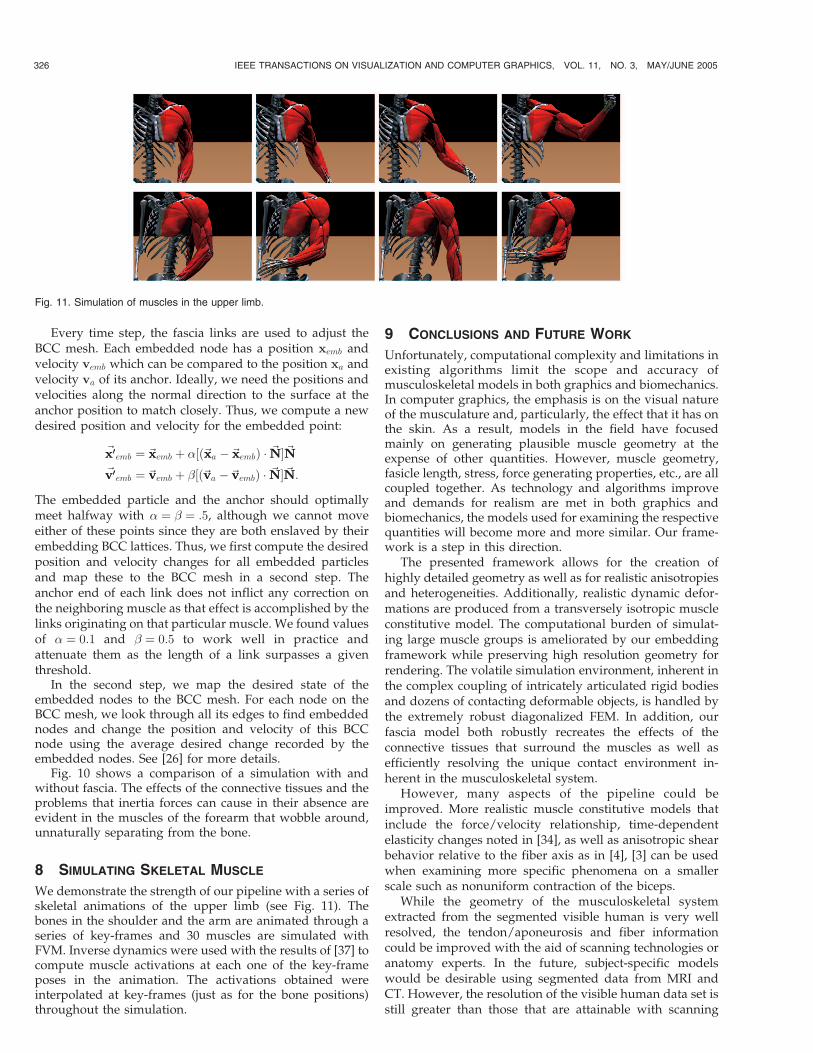
We demonstrate the strength of our pipeline with a series ofskeletal animations of the upper limb (see Fig. 11). Thebones in the shoulder and the arm are animated through aseries of key-frames and 30 muscles are simulated withFVM. Inverse dynamics were used with the results of [37] tocompute muscle activations at each one of the key-frameposes in the animation. The activations obtained wereinterpolated at key-frames (just as for the bone positions)throughout the simulation.

9 CONCLUSIONS AND FUTURE WORK

Unfortunately, computational complexity and limitations inexisting algorithms limit the scope and accuracy ofmusculoskeletal models in both graphics and biomechanics.In computer graphics, the emphasis is on the visual natureof the musculature and, particularly, the effect that it has onthe skin. As a result, models in the field have focusedmainly on generating plausible muscle geometry at theexpense of other quantities. However, muscle geometry,fasicle length, stress, force generating properties, etc., are allcoupled together. As technology and algorithms improveand demands for realism are met in both graphics andbiomechanics, the models used for examining the respectivequantities will become more and more similar. Our frame-work is a step in this direction.

The presented framework allows for the creation ofhighly detailed geometry as well as for realistic anisotropiesand heterogeneities. Additionally, realistic dynamic defor-mations are produced from a transversely isotropic muscleconstitutive model. The computational burden of simulat-ing large muscle groups is ameliorated by our embeddingframework while preserving high resolution geometry forrendering. The volatile simulation environment, inherent inthe complex coupling of intricately articulated rigid bodiesand dozens of contacting deformable objects, is handled bythe extremely robust diagonalized FEM. In addition, ourfascia model both robustly recreates the effects of theconnective tissues that surround the muscles as well asefficiently resolving the unique contact environment in-herent in the musculoskeletal system.

However, many aspects of the pipeline could beimproved. More realistic muscle constitutive models thatinclude the force/velocity relationship, time-dependentelasticity changes noted in [34], as well as anisotropic shearbehavior relative to the fiber axis as in [4], [3] can be usedwhen examining more specific phenomena on a smallerscale such as nonuniform contraction of the biceps.

While the geometry of the musculoskeletal systemextracted from the segmented visible human is very wellresolved, the tendon/aponeurosis and fiber informationcould be improved with the aid of scanning technologies oranatomy experts. In the future, subject-specific modelswould be desirable using segmented data from MRI andCT. However, the resolution of the visible human data set isstill greater than those that are attainable with scanning


Fig. 11. Simulation of muscles in the upper limb.

technologies. Thus, given the additional difficulty of

segmenting the scanned data, a reasonable alternative

approach is to use the model created from the visible

human data set and to deform (or morph) it to match a

specific subject or body type using anatomical landmarks

similar to [15].

ACKNOWLEDGMENTS

This research was supported in part by a US Office of NavalResearch (ONR) YIP award and a PECASE award (ONRN00014-01-1-0620), a Packard Foundation Fellowship, aSloan Research Fellowship, ONR N00014-03-1-0071, ONRN00014-02-1-0720, US Army Research Office (ARO)DAAD19-03-1-0331, US National Science Foundation(NSF) DMS-0106694, NSF ITR-0121288, NSF IIS-0326388,NSF ACI-0323866, NSF ITR-0205671, US National Institutesof Health (NIH) HD38962, and by Honda Research InstituteUSA. In addition, Joseph Teran and Silvia S. Blemker wereeach supported in part by an NSF Graduate ResearchFellowship and Eftychios Sifaki was supported by aStanford Graduate Research Fellowship.

REFERENCES

[1] A. Arnold, S. Blemker, and S. Delp, “Evaluation of a DeformableMusculoskeletal Model for Estimating Muscle-Tendon Lengthsduring Crouch Gait,” Computer-Aided Surgery, vol. 29, pp. 263-274,2001.

[2] A. Arnold and S. Delp, “Rotational Moment Arms of the MedialHamstrings and Adductors Vary with Femoral Geometry andLimb Position: Implications for the Treatment of InternallyRotated Gait,” J. Biomechanics, vol. 34, pp. 437-447, 2001.

[3] S. Blemker, “3D Modeling of Complex Muscle Architecture andGeometry,” PhD thesis, Stanford Univ., June 2004.

[4] S. Blemker, P. Pinsky, and S. Delp, “A 3D Model of MuscleReveals the Causes of Nonuniform Strains in the Biceps Brachii,”J. Biomechanics, 2004.

[5] J. Bonet and R. Wood, Nonlinear Continuum Mechanics for FiniteElement Analysis. Cambridge Univ. Press, 1997.

[6] R. Bridson, S. Marino, and R. Fedkiw, “Simulation of Clothingwith Folds and Wrinkles,” Proc. 2003 ACM SIGGRAPH/Euro-graphics Symp. Computer Animation, pp. 28-36, 2003.

[7] R. Bridson, J. Teran, N. Molino, and R. Fedkiw, “Adaptive PhysicsBased Tetrahedral Mesh Generation Using Level Sets,” 2004.

[8] J.T. Chang, J. Jin, and Y. Yu, “A Practical Model for Hair MutualInteractions,” Proc. ACM SIGGRAPH Symp. Computer Animation,pp. 77-80, 2002.

[9] D. Chen and D. Zeltzer, “Pump It Up: Computer Animation of aBiomechanically Based Model of Muscle Using the Finite ElementMethod,” Computer Graphics (SIGGRAPH Proc.), pp. 89-98, 1992.

[10] G. Debunne, M. Desbrun, A. Barr, and M-P. Cani, “InteractiveMultiresolution Animation of Deformable Models,” Proc. Euro-graphics Workshop Computer Animation and Simulation 1999, 1999.

[11] G. Debunne, M. Desbrun, M. Cani, and A. Barr, “Dynamic Real-Time Deformations Using Space & Time Adaptive Sampling,”Proc. SIGGRAPH 2001, vol. 20, pp. 31-36, 2001.

[12] G. Debunne, M. Desbrun, M.-P. Cani, and A. Barr, “AdaptiveSimulation of Soft Bodies in Real-Time,” Proc. Computer Animation2000, pp. 133-144, May 2000.

[13] S. Delp and J. Loan, “A Computational Framework for Simulatingand Analyzing Human and Animal Movement,” IEEE ComputingIn Science and Eng., vol. 2, no. 5, pp. 46-55, 2000.

[14] F. Dong, G. Clapworthy, M. Krokos, and J. Yao, “An Anatomy-Based Approach to Human Muscle Modeling and Deformation,”IEEE Trans. Visualization and Computer Graphics, vol. 8. no. 2, Apr.-June 2002.

[15] J. Fernandez, F. Mithraratne, S. Thrupp, M. Tawhai, and P.Hunter, “Anatomically Based Geometric Modeling of the Muscu-lo-Skeletal System and Other Organs,” Biomechanics and Modelingin Mechanobiology, vol. 3, 2003.

[16] T. Fukunaga, Y. Kawakami, S. Kuno, K. Funato, and S. Fukashiro,“Muscle Architecture and Function in Humans,” J. Biomechanics,vol. 30, 1997.

[17] B. Garner and M. Pandy, “A Kinematic Model of the Upper LimbBased on the Visible Human Project (VHP) Image Dataset,”Computer Methods in Biomechanics and Biomedical Eng., vol. 2,pp. 107-124, 1999.

[18] B. Garner and M. Pandy, “Musculoskeletal Model of the UpperLimb Based on the Visible Human Male Dataset,” ComputerMethods in Biomechanics and Biomedical Eng., vol. 4, pp. 93-126,2001.

[19] A.J.W. Gielen, P.H.M. Bovendeerd, and J.D. Janssen, “A ThreeDimensional Continuum Model of Skeletal Muscle,” ComputerMethods in Biomechanics and Biomedical Eng., vol. 3, pp. 231-244,2000.

[20] J.-P. Gourret, N. Magnenat-Thalmann, and D. Thalmann, “Simu-lation of Object and Human Skin Deformations in a GraspingTask,” Computer Graphics (SIGGRAPH Proc.), pp. 21-30, 1989.

[21] E. Grinspun, P. Krysl, and P. Schroder, “CHARMS: A SimpleFramework for Adaptive Simulation,” ACM Trans. Graphics(SIGGRAPH Proc.), vol. 21, pp. 281-290, 2002.

[22] G. Hirota, S. Fisher, A. State, C. Lee, and H. Fuchs, “An ImplicitFinite Element Method for Elastic Solids in Contact,” ComputerAnimation, 2001.

[23] G. Irving, J. Teran, and R. Fedkiw, “Invertible Finite Elements forRobust Simulation of Large Deformation,” Proc. 2004 ACMSIGGRAPH/Eurographics Symp. Computer Animation, pp. 131-140,2004.

[24] S. Jimenez and A. Luciani, “Animation of Interacting Objects withCollisions and Prolonged Contacts,” Modeling in ComputerGraphics–Methods and Applications, Proc. IFIP WG 5.10 WorkingConf., B. Falcidieno and T.L. Kunii, eds., pp. 129-141, 1993.

[25] A. Mohr and M. Gleicher, “Building Efficient, Accurate CharacterSkins from Examples,” ACM Transa. Graphics, vol. 22, no. 3,pp. 562-568, 2003.

[26] N. Molino, J. Bao, and R. Fedkiw, “A Virtual Node Algorithm forChanging Mesh Topology during Simulation,” ACM Trans.Graphics (SIGGRAPH Proc.), vol. 23, pp. 385-392, 2004.

[27] N. Molino, R. Bridson, J. Teran, and R. Fedkiw, “A Crystalline,Red Green Strategy for Meshing Highly Deformable Objects withTetrahedra,” Proc. 12th Int’l Meshing Roundtable, pp. 103-114, 2003.

[28] M. Muller, L. McMillan, J. Dorsey, and R. Jagnow, “Real-TimeSimulation of Deformation and Fracture of Stiff Materials,”Computer Animation and Simulation ’01, Proc. Eurographics Work-shop, pp. 99-111, 2001.

[29] V. Ng-Thow-Hing and E. Fiume, “Application-Specific MuscleRepresentations,” Proc. Graphics Interface 2002, W. Sturzlinger andM. McCool, eds., pp. 107-115, 2002.

[30] J. O’Brien and J. Hodgins, “Graphical Modeling and Animation ofBrittle Fracture,” Proc. SIGGRAPH ’99, vol. 18, pp. 137-146, 1999.

[31] S. Osher and R. Fedkiw, Level Set Methods and Dynamic ImplicitSurfaces. New York: Springer-Verlag, 2002.

[32] M. Pandy, “Moment Arm of a Muscle Force,” Exercise and SportScience Rev., vol. 27, 1999.

[33] G. Pappas, D. Asakawa, S. Delp, F. Zajac, and J. Drace, “Nonuni-form Shortening in the Biceps Brachii during Elbow Flexion,”J. Applied Physiology, vol. 92, no. 6, 2002.

[34] R. Schachar, W. Herzog, and T. Leonard, “Force Enhancementabove the Initial Isometric Force on the Descending Limb of theForce/Length Relationship,” J. Biomechanics, vol. 35, 2002.

[35] F. Scheepers, R. Parent, W. Carlson, and S. May, “Anatomy-BasedModeling of the Human Musculature,” Computer Graphics(SIGGRAPH Proc.), pp. 163-172, 1997.

[36] J. Sethian, “A Fast Marching Level Set Method for MonotonicallyAdvancing Fronts,” Proc. Nat’l Academy of Science, vol. 93, pp. 1591-1595, 1996.

[37] J. Teran, S. Blemker, V. Ng, and R. Fedkiw, “Finite VolumeMethods for the Simulation of Skeletal Muscle,” Proc. 2003 ACMSIGGRAPH/Eurographics Symp. Computer Animation, pp. 68-74,2003.

[38] D. Terzopoulos and K. Fleischer, “Modeling Inelastic Deforma-tion: Viscoelasticity, Plasticity, Fracture,” Computer Graphics(SIGGRAPH Proc.), pp. 269-278, 1988.

[39] D. Terzopoulos, J. Platt, A. Barr, and K. Fleischer, “ElasticallyDeformable Models,” Computer Graphics (Proc. SIGGRAPH ’87),vol. 21, no. 4, pp. 205-214, 1987.


[40] J. Tsitsiklis, “Efficient Algorithms for Globally Optimal Trajec-tories,” IEEE Trans. Automatic Control, vol. 40, pp. 1528-1538, 1995.

[41] US Nat’l Library of Medicine, “The Visible Human Project,” 1994,http://www.nlm.nih.gov/research/visible/.

[42] J. Weiss, B. Maker, and S. Govindjee, “Finite-Element Impementa-tion of Incompressible, Transversely Isotropic Hyperelasticity,”Computer Methods in Applied Mechanics and Eng., vol. 135, pp. 107-128, 1996.

[43] J. Wilhelms and A. Van Gelder, “Anatomically Based Modeling,”Computer Graphics (SIGGRAPH Proc.), pp. 173-180, 1997.

[44] C.A. Yucesoy, B.H. Koopman, P.A. Huijing, and H.J. Grootenboer,“Three-Dimensional Finite Element Modeling of Skeletal MuscleUsing a Two-Domain Approach: Linked Fiber-Matrix MeshModel,” J. Biomechanics, vol. 35, pp. 1253-1262, 2002.

[45] F. Zajac, “Muscle and Tendon: Properties, Models, Scaling, andApplication to Biomechanics and Motor Control,” Critical Reviewsin Biomedical Eng., vol. 17, no. 4, pp. 359-411, 1989.

[46] Q. Zhu, Y. Chen, and A. Kaufman, “Real-Time Biomechanically-Based Muscle Volume Deformation Using FEM,” ComputerGraphics Forum, vol. 190, no. 3, pp. 275-284, 1998.

Joseph Teran received the BS degree inmathematics from the University of California,Davis, in 2000 and and is currently pursuing thePhD degree in scientific computing at StanfordUniversity. His research interests include physi-cally-based animation, computational biomecha-nics, numerical methods for solids mechanics,and collision detection.

Eftychios Sifakis received the BSc degree incomputer science in 2000 and the BSc degree inmathematics in 2002 from the University ofCrete, Greece, and is currently pursuing thePhD degree in computer science at StanfordUniversity. He has published a number ofresearch papers in computer vision and imageanalysis. His current research focuses oncomputer graphics, physically-based simulation,and facial expression analysis.

Silvia S. Blemker received the BS and MSdegrees in biomedical engineering from North-western University, Evanston, Illinois, in 1997and 1999, respectively, and the PhD degree inmechanical engineering from Stanford Univer-sity, Stanford, California, in 2004. She iscurrently a research associate in the Bioengi-neering Department at Stanford University. Herresearch interests include neuromuscular bio-mechanics, movement disorders, musculoske-

letal modeling and simulation, medical imaging, and constitutivemodeling. She is a member of the American Society of Biomechanicsand the International Society for Magnetic Resonance in Medicine.

Victor Ng-Thow-Hing received the MSc andPhD degrees in computer science in 1994 and2001, respectively, from the University of Tor-onto, where he was a member of the DynamicsGraphics Project Lab. He is currently a researchscientist at the Honda Research Institute inMountain View, California. His research inter-ests include 3D muscle modeling, biomechanicalmusculoskeletal simulation, humanoid robotmotion skill acquisition, computational paleontol-

ogy, and software architectures for animation and simulation. He hasbeen a member of the program committee for the Symposium onComputer Animation since 2002 and has served as an executive boardmember of the International Society of Biomechanics Technical Groupon Computer Simulation since 2001.

Cynthia Lau received the BS in computerscience from Stanford University in 2004 andreceived the MS degree in computer sciencewith a systems specialization from Stanford inJanuary 2005. During her undergraduatestudies, she was awarded the President’sAward for Academic Excellence and member-ship in Phi Betta Kappa. As a graduatestudent, she participated in research in com-puter graphics with Professor Ronald Fedkiw

at Stanford University. She will be employed as a CoreTech softwareengineer at Adobe Systems, Inc. in San Jose, California, beginningin February 2005.

Ronald Fedkiw received the PhD degree inmathematics from the University of CaliforniaLos Angeles (UCLA) in 1996 and did postdoc-toral studies both at UCLA in mathematics andat Caltech in aeronautics before joining theStanford University Computer Science Depart-ment. He was awarded a Packard FoundationFellowship, a Presidential Early Career Awardfor Scientists and Engineers (PECASE), a SloanResearch Fellowship, a US Office of Naval

Research Young Investigator Program Award (ONR YIP), a Robert N.Noyce Family Faculty Scholarship, two distinguished teaching awards,etc. Currently, he is on the editorial board of the Journal of ScientificComputing, IEEE Transactions on Visualization and Computer Gra-phics, and Communications in Mathematical Sciences, and heparticipates in the reviewing process of a number of journals andfunding agencies. He has published more than 55 research papers incomputational physics, computer graphics, and vision, as well as a newbook on level set methods. For the past three years, he has been aconsultant with Industrial Light + Magic.

. For more information on this or any other computing topic,please visit our Digital Library at www.computer.org/publications/dlib.


ieee transactions on visualization and computer graphics, vol. 11

Documents