ieee transactions on signal processing 2 …bpence/bayes_estimation_gpc_for_peer... · recursive...

IEEE TRANSACTIONS ON SIGNAL PROCESSING 2

Recursive Bayesian state and parameter estimation

using polynomial chaos theoryBenjamin L. Pence, Jeffrey L. Stein, and Hosam K. Fathy.

Abstract—This paper joins polynomial chaos theory withBayesian estimation to recursively estimate the states and un-known parameters of asymptotically stable, linear, time invariant,state-space systems. This paper studies the proposed algorithmsfrom a pole/zero locations perspective. The estimator has fixedpole locations that are independent of the estimation algorithm(and the estimated variables). Only the estimator zero locationsare affected by estimation. This paper uses a 3rd order differen-tial equation to study the behavior of the proposed estimator.It uses pole/zero maps and Bode plots to observe how thepolynomial chaos based estimators vary the system zero locationsto make the expanded polynomial chaos output most like (in someBayesian sense) the 3rd order system output.

Index Terms—Estimation, Bayesian Inference, Poles and Zeros,Bode Plot, Polynomial Chaos Theory.

I. INTRODUCTION

THIS paper combines generalized polynomial chaos theory

[1] with Bayesian estimation (see Chapter 12 of [2])

for a recursive solution to parameter and state (including

initial state) estimation in state space systems. Because of the

Bayesian estimation framework, this paper’s methods are able

to recursively calculate statistical characteristics (e.g., standard

deviation, confidence intervals) of the parameter estimates as

well as the most likely parameter values. This is an advantage

compared to earlier estimators by the authors [3] and [4] which

used the maximum likelihood estimation framework.

As a fundamental property, the proposed estimator has fixed

pole locations but variable zero locations. Polynomial chaos

theory determines the (fixed) estimator pole locations. Hence,

the estimator pole locations are independent of the estimated

variables. The estimation algorithm varies only the zero loca-

tions to calculate the estimates of the unknown parameters and

states. To help illustrate this fundamental property, Section 5

uses a simulation example to study the proposed estimators

from a frequency domain and pole/zero locations perspective.

State filtering approaches [5] such as extended Kalman

filtering, unscented Kalman filtering, and particle filtering,

may also be used to recursively estimate the unknown pa-

rameters and states of state space systems. To estimate the

system parameters, these state-filtering approaches treat the

unknown static parameters as dynamic states (usually with

zero dynamics). This generally increases the nonlinearity of

the system. In the proposed approach of this paper, linearity

is preserved. In some cases, the methods of this paper may be

B. L. Pence is with the Department of Mechanical Engineering, Universityof Michigan, Ann Arbor, MI, 48109 USA e-mail: [email protected].

H. K. Fathy is with Pennsylvania State University, and J. L. Stein is withthe University of Michigan.

easier to tune than the state filtering approaches [3]. As another

advantage, the proposed approach has the ability to treat

unknown initial states as estimation parameters and update

their values recursively as new data arrive. Perhaps the main

limitation of the proposed approach, however, relates to its

computational demand, especially for systems with a large

number of unknown parameters.

The following paragraphs review existing approaches that

use polynomial chaos theory as a framework for estimating

unknown parameters of dynamic state space systems. This

review groups the various estimators into 4 categories: (a) non-

recursive or batch estimators, (b) recursive observer/Kalman

filter based estimators, (c) recursive instantaneous cost esti-

mators, and (d) recursive Bayesian or maximum likelihood

estimators (without observers/Kalman filters) - the approach

of this paper fits into this last category.

Batch estimators calculate estimates of unknown parameters

by evaluating an entire set or batch of data as opposed to

updating the estimates iteratively as data arrive. Blanchard

et al. proposed a batch Bayesian parameter estimator for

linear and nonlinear state space systems that selects estimates

based on the maximum a posteriori criterion [6]. Another

batch estimator proposed by Blanchard et al. [7] called the

“whole-set-of-data-at-once” approach, combines polynomial

chaos theory with the extended Kalman filter. Blanchard

et al. report that the “whole-set-of-data-at-once” approach

yields better results than the recursive or so-called “one-

time-step-at-a-time” approach also developed by Blanchard et

al. Marzouk and Xiu [8] proposed a Bayesian approach to

estimate parameters of systems governed by partial differential

equations; they provided a valuable study on the convergence

of the polynomial chaos based estimators. Their work used

the stochastic collocation approach and extended earlier but

similar work [9] which used the Galerkin method.

Recursive estimators calculate system parameters iteratively

as new data arrive. Polynomial chaos theory has been com-

bined with state observers to recursively predict estimates of

the system states and then update the state predictions when

measurements of the output signals become available. These

observers can also estimate unknown system parameters if

the unknown parameters are explicitly treated as dynamic

system states. Blanchard et al. combined polynomial chaos

theory with the extended Kalman filter for state and parameter

estimation [7]. Li and Xiu proposed a polynomial chaos based

ensemble Kalman filter [10]. Saad et al. also proposed a

polynomial chaos based ensemble Kalman filter for system

identification and monitoring [11], and Smith et al. [12] com-

bined polynomial chaos theory with the Luenberger observer


for state estimation.

Southward developed a unique framework for recursive

parameter estimators based on polynomial chaos theory [13].

Southward’s method recursively calculates parameter esti-

mates by searching in the direction of gradients of instan-

taneous quadratic cost functions. Shimp [14] and the authors

[15] applied Southward’s method to the problem of real-time

vehicle mass estimation.

The proposed algorithms of this paper recursively seek

parameter estimates that satisfy some Bayesian optimality

criteria. However, they do not use state observers or Kalman

filters like the methods above. Instead, polynomial chaos

theory propagates parametric uncertainty through the dynamic

system, and Bayesian estimation theory is applied directly to

the stochastic system output to calculate parameter estimates.

Dutta and Bhattacharya also proposed a Bayesian estimator

based on polynomial chaos theory [16]. Unlike the methods of

this paper, however, their estimator requires the inner products

in the estimation algorithm to be recomputed at each time

step. The authors proposed a maximum likelihood approach to

recursive parameter estimation using polynomial chaos theory

in [3]. This paper extends the earlier work by the authors

but uses the Bayesian framework instead of the maximum

likelihood framework.

The following section provides an overview of generalized

polynomial chaos theory. Section 3 discusses pole/zero char-

acteristics of the proposed estimator. Section 4 derives the

recursive estimation algorithms. Section 5 uses an example

system with pole/zero maps and Bode plots to study the

proposed estimators, and Section 6 provides a summary and

conclusions.

II. GENERALIZED POLYNOMIAL CHAOS (GPC) THEORY

The generalized polynomial chaos (gPC) framework is

essential to the methods of this paper. It is already well-

established in the literature and is not considered a contribution

of this paper; a summary for linear systems is presented

here, however, to provide a foundation for the proposed

contributions. The gPC framework was developed by Xiu and

Karniadakis [1] building on groundbreaking work by Ghanem

and Spanos [17] and the conceptualization by Wiener [18].

Consider the following Linear-Time-Invariant (LTI), state-

equations:

x = Ax+Bu (1)

x(0) = x0. (2)

The vector x ∈ Rns contains the system states which have

initial conditions x0. The matrices A ∈ Rns×ns and B ∈

Rns×nu and the initial state vector x0 may be functions of

an unknown parameter vector θ ∈ Rnp . The input vector u ∈

Rnu is known and time-varying. The “dot” notation signifies

the derivative with respect to time t. This paper assumes that

the state equations are asymptotically stable for all possible

realizations of θ.

The output yk ∈ Rny is described by a linear, time-invariant,

discrete-time equation:

yk = Cx(tk) + vk. (3)

The output vector yk contains the observations on the

system at time tk. The matrix C ∈ Rny×ns may be a function

of the unknown parameters θ. The vector vk ∈ Rny represents

a Gaussian noise sequence with known covariance matrix

Rk ∈ Rny×ny .

The unknown parameters are viewed as being functions of

chaos (random) variables ξ = [ξ1 ξ2 . . . ξnp], i.e., θ = θ(ξ).

The chaos variables ξi are independently identically distributed

(IID), and the joint density function is ρ(ξ) =∏np

i=1 ρ(ξi)where ρ(ξi) is the distribution of the ith random variable

ξi. Parametric uncertainty leads to uncertainty in the system

states. Therefore, x(t) = x(t, ξ) is also a function of the chaos

variables.

Using the gPC framework, the unknown parameters θ(ξ)and system states x(t, ξ) are expanded in terms of orthogonal

polynomial basis functions Φα(ξ) : Rnp → R.

θ(ξ) =S∑

|α|=0

θαΦα(ξ) =r

∑

i=0

θiΦi(ξ), (4)

x(t, ξ) =

S∑

|α|=0

xα(t)Φα(ξ) =r

∑

i=1

xi(t)Φi(ξ). (5)

The expansion coefficients for the unknown parameters are

θi ∈ Rnp . The state expansion coefficients are xi(t) : R

+ →R

ns . Here, the vector α := [α1, . . . , αnp] is an np-dimensional

multi-index, and |α| is the sum of the vector elements, i.e.

|α| = α1 + . . . + αnp. Each element αi, i = 1, . . . , np of α

can take on a non-negative integer value between 0 and S. The

purpose of the second summation in (4) and (5) is to show

that the total number, r, of terms in the expansion is generally

not S + 1, rather it is calculated by (see [1]):

r =(S + np)!

S!np!. (6)

Under certain assumptions (see [1]), Equations (4) and

(5) become exact in the L2 sense as S → ∞. An infinite

expansion is not computationally attainable, so truncation is

necessary, and (4) and (5) are, in general, only approximations.

The paper by Xiu and Karniadakis [1] suggests how to select

the basis functions Φi(ξ). The parameter expansion coeffi-

cients θi, i = 1, . . . , r are chosen such that the distribution

of the parameter expansion (4) is the closest approximation to

the prior distribution ρ(θ) in some sense (e.g., by matching

certain statistical moments). Therefore, θi is known for all

i. Polynomial chaos theory solves for the coefficients xi(t)of the polynomial chaos state expansion (5) via the Galerkin

approach [17]. The Galerkin approach solves for the expansion

coefficients xi(t) by projecting the expanded state equations -

equations resulting from substituting (4) and (5) into (1) and

(2) - onto the polynomial chaos basis functions Φi(ξ) i.e.,

〈 ˙x(t, ξ), Φi(ξ)〉 = 〈A(ξ)x(t, ξ) +B(ξ)u(t), Φi(ξ)〉,

〈x(0), Φi(ξ)〉 = 〈x0, Φi(ξ)〉, i = 1, . . . , r. (7)

This projection removes the dependence on ξ, and the

resulting deterministic state equations have the state-expansion

coefficients xi(t) as the new state variables. The inner product


〈F (ξ), G(ξ)〉 is an np-dimensional integral of the product of

F (ξ) and G(ξ), evaluated over the event space of the random

variables ξ:

〈F (ξ), G(ξ)〉 :=

∫

G(ξ)F (ξ)W (ξ)dξ. (8)

The weighting function W (ξ) depends on the choice of

polynomial basis functions, and is generally equal to the prior

distribution ρ(ξ) of the chaos variables ξ [1].

The state-expansion of Equation (5) can be written as

the following matrix-vector product with the elements of

the vector state-expansion coefficients xi(t), i = 1, . . . , r as

elements of a single column vector X(t) (see [3]):

x(t, ξ) = P(ξ)X(t). (9)

In summary, applying the Galerkin projection (7) results in

r independent sets of deterministic state-equations. Evaluating

the deterministic dynamic equations results in known trajecto-

ries of the time dependent state-coefficients xi(t), i = 1, . . . , rwhich are then recombined - using (9) or (5) - with the random

variable dependent parts Φi(ξ), i = 1, . . . , r to obtain the

complete stochastic solution x(t, ξ).

III. POLES AND ZEROS OF GPC EXPANDED SYSTEMS

The r independent sets of deterministic state-equations can

be combined into one system of equations. The resulting set

of state equations is linear and time invariant:

X = AgPCX +BgPCu. (10)

The matrices AgPC ∈ Rrns×rns and BgPC ∈ R

rns×nu and

the initial conditions X(0) follow from Equation (7). This

polynomial chaos expanded system, Equation (10), is not a

function of ξ, but is deterministic.

The pole locations of the proposed estimator are the com-

plex eigenvalues of AgPC . They are fixed, i.e., they are

independent of ξ, and they are independent of the estimated

value of ξ.

The state equations are deterministic, but the polynomial

chaos output equation is a function of ξ:

yk(ξ) = CgPC(ξ)X(tk). (11)

Here CgPC(ξ) : Rnp → R

ny×rns is defined as CgPC(ξ) :=C(θ(ξ))P (ξ), where θ(ξ) is replaced by its polynomial chaos

expansion (4). Because the output equation is a function of

ξ, the zero locations of the polynomial chaos system are

functions of ξ (see page 15 of [19]). The proposed estimation

approach seeks the value of ξ, i.e. ξk, such that the polynomial

chaos system output yk(ξk) ∈ Rny is most like the true

system output yk in some optimal Bayesian sense (maximum

a posteriori or minimum mean squared error).

IV. RECURSIVE PARAMETER ESTIMATION

This section derives the recursive parameter update laws

for estimating the values of the random variables ξ given the

system output observations. The estimates of the unknown

parameters θ(ξ) are then calculated using (4) and the state

estimates are calculated using (5) or (9). Optimal Bayesian

estimation requires that the polynomial chaos approximations

in (4) and (5) are exact. As mentioned above, this requirement

is satisfied as the number of expansion terms goes to infinity

[1] (see also [8] and [9]). In practice, the expansion must be

truncated after a finite number of terms, and thus the parameter

estimates via this method are suboptimal.

Bayes rule [20] describes how a prior parameter distribution

ρ(ξ) : Rnp → R of a random vector ξ ∈ R

np evolves to

its posterior parameter distribution ρ(ξ|y0:k) : Rnp → R. The

posterior distribution ρ(ξ|y0:k) is conditioned on all of the sys-

tem observations y0:k up through time tk. One representation

of Bayes rule is as follows:

ρ(ξ|y0:k) =1

∫

L(ξ|y0:k)ρ(ξ)dξL(ξ|y0:k)ρ(ξ). (12)

The function L(ξ|y0:k) : Rnp → R is the likelihood

function, and for additive Gaussian noise assumptions, it is

defined as follows (see Chapter 12 of [2]):

L(ξ|y0:k) =k∏

τ=0

ρ(yτ |ξ)

∝ exp{−1

2

k∑

τ=0

(yτ − yτ (ξ))TR−1

τ (yτ − yτ (ξ))}. (13)

Here, L(ξ|y0:k) : Rnp → R is the scalar likelihood at

time tk of the unknown parameters ξ conditioned on y0:k.

The function ρ(yk|ξ) is the conditional probability of the

observation yk at time tk given ξ. In general, yk ∈ Rny

is the argument of ρ(yk|ξ), but in calculating the likelihood

(13), ξ becomes the argument of ρ(yk|ξ) : Rnp → R and

yk is assumed to be given. The vector yk(ξ) ∈ Rny is the

output of the stochastic model (11). The maximum likelihood

estimate ξ is the realization of ξ that maximizes the likelihood

function (13). The maximum likelihood estimation approach

was studied in [3]. If the time summation in the exponent

of (13) can be calculated iteratively, the likelihood function

(13) and hence the Bayesian posterior density (12) can also

be calculated iteratively. The time summation in the exponent,

i.e., the negative log-likelihood, can be written as follows [4]:

Jk(ξ) :=1

2

k∑

τ=0

(yτ − yτ (ξ))TR−1

τ (yτ − yτ (ξ)). (14)

The earlier work by the authors [3] describes how to cal-

culate Jk(ξ) : Rnp → R iteratively. Polynomial chaos theory

and the linearity of the output model (3) enable separation

of the time and unknown parameter parts of the equation to

make this recursion possible. By substituting (11) into (14)

and performing a few algebraic manipulations, the function

Jk(ξ) can be written as:

Jk(ξ) =1

2

ny∑

i=1

ny∑

j=1

(Dy(i)y(j)

k − 2C(i)gPCD

Xy(j)

k

+ C(i)gPCD

XXT

k (C(j)gPC)

T ). (15)

In Equation (15), the term DGk is defined

as DGk :=

∑k

τ=0[R−1τ ](i,j)Gτ where Gk ∈


{y(i)k y

(j)k , X(tk)y

(j)k , X(tk)(X(tk))

T }. The scalar term

[R−1k ](i,j) is the jth element in the ith row of the inverse

covariance matrix R−1k . Also, the scalar y(l) is the lth element

of the observation vector yk and C(l)gPC is the lth row of

the output matrix CgPC(ξ). Equation (15) can be updated

recursively from time tk to tk+1 since DGk+1 = DG

k +Gk+1,

and Gk is not a function of ξ. Hence, using (15), the

Bayesian posterior distribution can be calculated recursively

and evaluated at time tk for any realization of ξ; it can be

written in terms of the function Jk(ξ) as follows:

ρ(ξ|y0:k) =1

∫

exp{−Jk(ξ)}ρ(ξ)dξexp{−Jk(ξ)}ρ(ξ). (16)

Given the posterior density, the estimate of ξ is found by

calculating either the Minimum Measn Squared Error (MMSE)

estimate or the Maximum A Posteriori (MAP) estimate. The

MMSE estimate of the parameter vector ξ is calculated as

follows (see pages 350-354 of [21]):

ξ(MMSE)k = E{ξ|y0:k}

=1

∫

exp{−Jk(ξ)}ρ(ξ)dξ

∫

exp{−Jk(ξ)}ρ(ξ)dξ. (17)

Both np-dimensional integrals in (17) are integrated over the

event space of ξ. Because these integrals must be evaluated at

each time step, the MMSE estimator is more computationally

demanding than the MAP estimator. Monte Carlo integration

(see Section 6.12 of [22]) or other numerical integration

techniques can be applied to evaluate these integrals.

The MAP estimate of the unknown parameter vector ξ is

the realization of ξ that maximizes the posterior distribution

ρ(ξ|y0:k). Since the denominator of (16) is constant with

respect to ξ, the MAP estimator is given by

ξ(MAP )k = argmax

ξ

exp{−Jk(ξ)}ρ(ξ). (18)

Using the monotonic property of the logarithm function, the

MAP estimator also satisfies the following equation [20]:

ξ(MAP )k = argmin

ξ

{Jk(ξ)− log(ρ(ξ))}. (19)

The same recursive optimization strategies used in [3] for

maximizing the likelihood function can also be applied in this

paper to minimize Jk(ξ) − log(ρ(ξ)) and hence recursively

calculate ξ(MAP )k .

Higher order moments of the estimated posterior distribution

ρ(ξ|y0:k) can also be calculated. The mth moment is calcu-

lated as follows:

E{ξm|y0:k}

=1

∫

exp{−Jk(ξ)ρ(ξ)dξ

∫

ξm exp{−Jk(ξ)}ρ(ξ)dξ. (20)

These higher order moments provide valuable information

characterizing the statistical posterior distribution of the un-

known parameters. For example, the posterior variance is

calculated using the MMSE estimate and the second order

moment by var(ξ) = E{ξ2|y0:k} − (ξ(MMSE)k )2. Like the

MMSE estimate, calculations of the higher order moments

require evaluating integrals at each time step and thus require

more computational resources.

Because of polynomial chaos theory, the Bayesian posterior

density can be calculated recursively. Numerical integration

calculates MMSE estimates of ξ, and/or optimization strategies

calculate MAP estimates of ξ. State and parameter estimates

follow from Equations (4) and (5).

V. EXAMPLE

This section uses a third order differential equation to study

the proposed estimator from a pole/zero locations perspective.

For simplicity, this example only considers one unknown

parameter. The third order system is as follows:

x = Atx+BTu

yk = CTx(tk) + vk

AT :=

0 0 −11 0 −20 1 −a2

, BT :=

110

CT :=[

0 0 1]

(21)

This system of equations is asymptotically stable for a2 >1/2. This example assumes that the true value for a2 is

unknown, however, prior knowledge suggests that a2 could be

any value between 1 and 10 with equal probability. The mea-

sured (and hence known) input u is generated using a Gaussian

sequence generator with zero mean and unit variance. The

unknown noise sequence vk is generated using a Gaussian

sequence generator with zero mean and 0.0006 variance. This

corresponds to a signal-to-noise ratio (variance of yk − vkdivided by variance of vk) of 4.0.

Because the prior distribution of a2 is uniform, the ex-

pansion polynomials Φi(ξ), i = 1, . . . , r are the Legendre

polynomials (see [1], [23]) and the prior distribution of ξis uniform over the interval [−1, 1]. A Legendre polynomial

chaos expansion of the system of Equation (21) results in the

following expanded system of equations in which the state vec-

tor X contains the polynomial chaos expansion coefficients:

X = AgPCX +BgPCu

yk(ξ) = CTP(ξ)X(tk)

AgPC :=

07×7 07×7 −I7I7 07×7 −2I7

07×7 I7 −A33

BgPC :=

106×1

1013×1

CT :=[

0 0 1]

P(ξ) :=

Φ1 · · ·Φr 0 · · · 0 0 · · · 00 · · · 0 Φ1 · · ·Φr 0 · · · 00 · · · 0 0 · · · 0 Φ1 · · ·Φr

(22)

The highest order of the Legendre polynomials in the poly-

nomial chaos expansion was chosen (somewhat arbitrarily) to


be six, hence there are seven expansion terms (i.e. r = 7) per

original state resulting in a total of 21 states in the expanded

system (22). An ad hoc approach to determine an acceptable

value for the polynomial order is to start with a small value

and then iterate until the change in the resulting parameter

estimates between iterations is acceptably small. The term I7is the 7 × 7 identity matrix and 0j×l is the zero matrix with

dimensions j × l. The term A33 is calculated as follows:

A33

= Adiag

〈Φ1, a2Φ1〉〈Φ1, a2Φ2〉 · · · 〈Φ1, a2Φ7〉〈Φ2, a2Φ1〉〈Φ2, a2Φ2〉 · · · 〈Φ2, a2Φ7〉

......

. . ....

〈Φ7, a2Φ1〉〈Φ7, a2Φ2〉 · · · 〈Φ7, a2Φ7〉

Adiag =

δ1 0 · · · 00 δ2 · · · 0...

.... . .

...

0 0 · · · δ7

δi = 〈Φi,Φi〉−1. (23)

Note that a2 = 11/2 + 9ξ/2 is an exact polynomial chaos

expansion of a2 in the sense that the prior distributions of a2and a2 are identically distributed between 1 and 10. Thus only

two polynomial chaos expansion terms are needed to represent

a2 exactly (see Equation (4)).

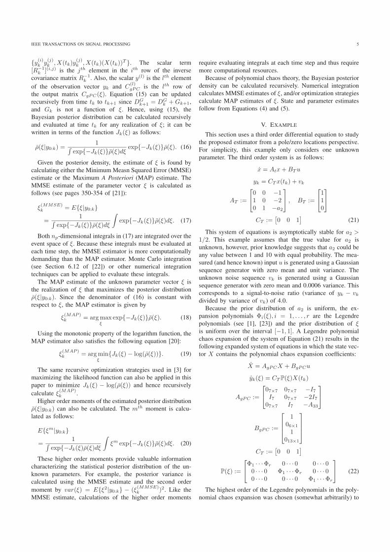
The matrix AgPC and its eigenvalues are deterministic. The

eigenvalues of AgPC are the poles of the polynomial chaos

system of Equation (22). Figure 1 shows these pole locations

on the same graph as a root locus plot of the pole locations of

the original 3rd order system of Equation (21) for all possible

values of a2 ∈ [1, 10]. For this example, the poles of the

polynomial chaos system (generated automatically using the

Galerkin projection) land almost exactly on top of the locus of

the original system. This result is independent of the estimated

value of ξ.

A. Output Disturbance Only

The square markers in Figure 1 show the pole locations for

the 3rd order system for the choice a2 = 3.6737. Admittedly,

this choice is contrived so that the 3rd order system poles

correspond almost exactly - accurate to at least 4 decimal

places - to three of the polynomial chaos system poles.

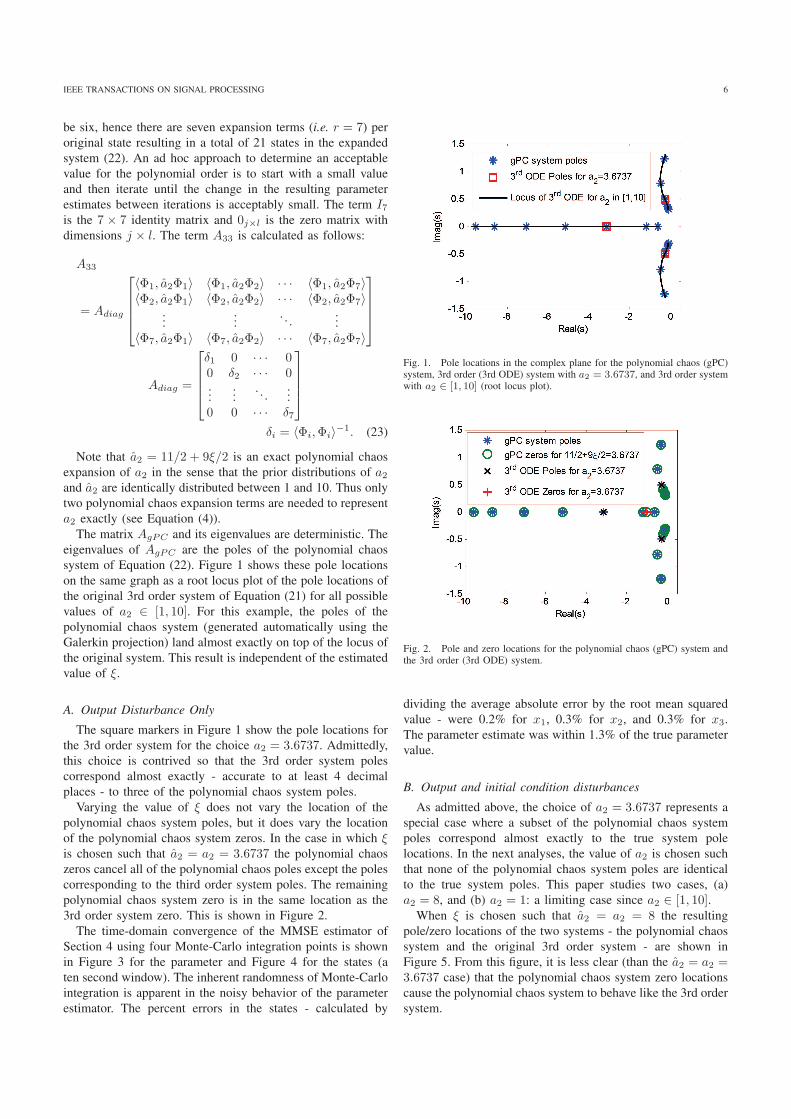
Varying the value of ξ does not vary the location of the

polynomial chaos system poles, but it does vary the location

of the polynomial chaos system zeros. In the case in which ξis chosen such that a2 = a2 = 3.6737 the polynomial chaos

zeros cancel all of the polynomial chaos poles except the poles

corresponding to the third order system poles. The remaining

polynomial chaos system zero is in the same location as the

3rd order system zero. This is shown in Figure 2.

The time-domain convergence of the MMSE estimator of

Section 4 using four Monte-Carlo integration points is shown

in Figure 3 for the parameter and Figure 4 for the states (a

ten second window). The inherent randomness of Monte-Carlo

integration is apparent in the noisy behavior of the parameter

estimator. The percent errors in the states - calculated by

Fig. 1. Pole locations in the complex plane for the polynomial chaos (gPC)system, 3rd order (3rd ODE) system with a2 = 3.6737, and 3rd order systemwith a2 ∈ [1, 10] (root locus plot).

Fig. 2. Pole and zero locations for the polynomial chaos (gPC) system andthe 3rd order (3rd ODE) system.

dividing the average absolute error by the root mean squared

value - were 0.2% for x1, 0.3% for x2, and 0.3% for x3.

The parameter estimate was within 1.3% of the true parameter

value.

B. Output and initial condition disturbances

As admitted above, the choice of a2 = 3.6737 represents a

special case where a subset of the polynomial chaos system

poles correspond almost exactly to the true system pole

locations. In the next analyses, the value of a2 is chosen such

that none of the polynomial chaos system poles are identical

to the true system poles. This paper studies two cases, (a)

a2 = 8, and (b) a2 = 1: a limiting case since a2 ∈ [1, 10].When ξ is chosen such that a2 = a2 = 8 the resulting

pole/zero locations of the two systems - the polynomial chaos

system and the original 3rd order system - are shown in

Figure 5. From this figure, it is less clear (than the a2 = a2 =3.6737 case) that the polynomial chaos system zero locations

cause the polynomial chaos system to behave like the 3rd order

system.


Fig. 3. Convergence of the MMSE estimator for the parameter a2.

The hypothesis that zero placement causes the polynomial

chaos system to behave like the 3rd order system is verified

from a Bode plot comparison of the two systems. The Bode

plots of the two systems are shown in Figure 6.

The time-domain convergence of the proposed MAP es-

timator of Section 4 is shown in Figure 7 and Figure 8.

In this simulation experiment, an additional disturbance was

introduced: the initial value of x3 was set to one (unknown

to the estimator which assumes that x3(0) = 0). The transient

performance of the estimator was affected, but as expected

(see Appendix A1 of [24]), the steady-state performance was

relatively unaffected as seen in Figure 7 and Figure 8. Figure 7

and Figure 8 show the convergence of the proposed MAP

estimator for two cases: (a) the estimator knows about the

initial condition disturbance x3(0) = 1, and (b) the estimator

erroneously assumes all initial conditions are zero. Even with

the unknown initial condition disturbance, the largest average

error in the state estimates was less than 4%. The parameter

estimate converged to within less than 1% of the true value.

C. Output and input (state) disturbances

When ξ is chosen such that a2 = a2 = 1 the resulting

pole/zero locations of the two systems are shown in Figure 9.

A Bode plot comparing the two systems is shown in Figure 10.

The Bode plots of the two systems do not match as well in

the frequency range [0.5, 2] radians per second as at other

Fig. 4. True and estimated states in the window [60, 70] seconds.


frequencies. However, the polynomial chaos system closely

matches the original 3rd order system at most frequencies.

This result (and the authors’ experience in general) suggests

that the performance of the polynomial chaos based estimators

degrades near the limits (especially for systems with multiple

unknown parameters).

The time-domain convergence of the proposed MMSE es-

timator of Section 4 is shown in Figure 11 and Figure 12.

In this simulation experiment, an additional disturbance - this

time on the input signal - was introduced. The true system

input was u as usual, but the measured signal (i.e. the signal


Fig. 6. Bode plot of the 3rd order (3rd ODE) and polynomial chaos systemsfor a2 = a2 = 8.

Fig. 7. Parameter convergence of the MAP estimator under the assumptionsx3(0) = 1 (solid line) and x3(0) = 0 (dotted line). The true initial conditionwas x3(0) = 1. The dashed line shows the true parameter value.

used by the estimator) was u + w. The noise sequence wwas generated using a Gaussian sequence generator with zero

mean and variance 0.25. This corresponds to an input signal-

Fig. 8. True and estimated states under the assumptions x3(0) = 1 (dot-dashline) and x3(0) = 0 (solid line). The true initial condition was x3(0) = 1.The dashed line corresponds to the true states.


to-noise ratio of four (variance of u divided by variance of

w). Figure 11 and Figure 12 show the convergence of the

parameter and state estimators for two cases: (a) without the


Fig. 10. Bode plot of the true (3rd ODE) system and the polynomial chaos(gPC) system.

added disturbance w, and (b) with the added disturbance w.

The largest average error, 22%, is in the estimate of state x2

under the input disturbance w. Without the input disturbance

the error in state x2 is about 13%. Even without the additional

disturbance w, the errors for this (limiting) case are greater

than for the previous cases in Sections 4.1 and 4.2. The

parameter estimate converged within 1% of the true value.

VI. CONCLUSION

This paper used polynomial chaos theory to derive new re-

cursive approaches to Bayesian state and parameter estimation

of linear time-invariant systems. It used a pole/zero and Bode

plot analysis to study the proposed estimators for a 3rd order

system with one unknown parameter. This study observed

that the expanded polynomial chaos system had eigenvalues

located on the root locus of the original 3rd order system.

The proposed estimator selected realizations of the unknown

parameter to strategically place the polynomial chaos system

zeros. This zero placement caused the higher order polynomial

chaos system to closely match the 3rd order system (as seen

in the Bode plots and the pole/zero maps). This paper showed

the convergence of the polynomial chaos estimator for the

state and parameter estimates under three different types of

disturbances: output signal noise only, output signal noise plus

initial condition disturbances, and output signal noise plus

input signal noise (i.e. state disturbances). In each case, the

parameter estimate converged to within less than 10% error.

APPENDIX

A COMMENT ON NUMERICAL IMPLEMENTATION

This section provides a useful note on numerical imple-

mentation of the MMSE and higher-order-moments estimators

Equations (17) and (20) respectively. First note, however, that

the MMSE estimator of (17) is a special case of the higher

Fig. 11. Parameter convergence for two cases: output disturbance only (Solidline) and output and input disturbance (dotted line). The dashed line showsthe true parameter value.

order moment estimator of (20) with m = 1. Therefore, the

same numerical techniques that apply to (20) also apply to

(17). The difficulty in numerically evaluating Equations (17)

and (20) is as follows: because the objective function Jk(ξ) is

essentially the summation over time of the squared difference

between y and y (see Equation (14)), its value may tend to

positive infinity as time increases. The exponential functions

in (17) and (20) quickly (exponentially) converge to zero as

the magnitude of Jk(ξ) increases. Thus, the integrals in the

numerator and denominator of (17) and (20) quickly become

smaller than the precision of the computer, and Equations (17)

and (20) have the numerical problem of dividing zero by zero.

To avoid this issue of dividing zero by zero, this section for-

mulates Equation (20) in the following manner by multiplying

by one:

E{ξm|y0:k}

=

∫

ξm exp{−Jk(ξ)}ρ(ξ)dξ∫

exp{−Jk(ξ)}ρ(ξ)dξ

exp{Jk(ξ(MMSE)k−1 )}

exp{Jk(ξ(MMSE)k−1 )}

. (24)

Here, Jk(ξ(MMSE)k−1 ) is the current cost of the previous

MMSE estimate ξ(MMSE)k−1 . The term exp{Jk(ξ

(MMSE)k−1 )}

is constant with respect to ξ and can be moved inside the


Fig. 12. True and estimated states. The dot-dash line is for output disturbanceonly. The solid line is for both output and input (state) disturbances. Thedashed line is the true state.

integrals of (24). The equation can then be written

E{ξm|y0:k}

=

∫

ξm exp{−Jk(ξ) + Jk(ξ(MMSE)k−1 )}ρ(ξ)dξ

∫

exp{−Jk(ξ) + Jk(ξ(MMSE)k−1 )}ρ(ξ)dξ

. (25)

The term in the exponent −Jk(ξ) + Jk(ξ(MMSE)k−1 ) is small

for some ξ (its value is zero for ξ = ξ(MMSE)k−1 and thus

Equation (25) avoids the problem of dividing zero by zero

assuming ξ(MMSE)k−1 is one of the numerical integration points.

REFERENCES

[1] D. Xiu and G. Karniadakis, “The wiener-askey polynomial chaos forstochastic differential equations,” SIAM J. on Scientific Computing,vol. 24, pp. 619–644, 2002.

[2] T. Moon and W. Stirling, Mathematical Methods and Algorithms for

Signal Processing. New Jersey: Prentice-Hall, Inc, 2000.[3] B. Pence, H. Fathy, and J. Stein, “Recursive maximum likelihood

parameter estimation for state space systems using polynomial chaostheory,” Automatica, vol. (accepted, preprint available at http://www-personal.umich.edu/ bpence/), 2011.

[4] ——, “A maximum likelihood approach to recursive polynomial chaosparameter estimation,” in Proc. 2010 American Control Conference -

ACC 2010, Baltimore, MD, USA, 30 June-2 July 2010.[5] D. Simon, Optimal State Estimation: Kalman, H infinity, and Nonlinear

Approaches. New Jersey: John Wiley and Sons Inc., 2006.[6] E. Blanchard, A. Sandu, and C. Sandu, “A polynomial-chaos-based

bayesian approach for estimating uncertain parameters of mechanicalsystems,” 19th Int. Conf. on Des. Theory and Method.; 1st Int. Conf.

on Micro- and Nanosys.; and 9th Int. Conf. on Adv. Vehicle Tire Tech.,

Parts A and B, vol. 3, pp. 1041–1048, 2008.[7] ——, “A polynomial chaos-based kalman filter approach for parameter

estimation of mechanical systems,” Paper no. 061404, ASME J. of

Dynamic Systems Measurement and Control, Special Issue on Physical

System Modeling, vol. 132, 2010.[8] Y. Marzouk and D. Xiu, “A stochastic collocation approach to bayesian

inference in inverse problems,” Comm. in Comp. Physics, vol. 6, pp.826–847, 2009.

[9] Y. Marzouk, N. Najm, and L. Rahn, “Stochastic spectral methods forefficient bayesian solution of inverse problems,” J. Comp. Physics, vol.224, pp. 560–586, 2007.

[10] J. Li and D. Xiu, “A generalized polynomial chaos based ensemblekalman filter with high accuracy,” J. of Comp. Physics, vol. 228, pp.5454–5694, 2009.

[11] G. Saad, R. Ghanem, and S. Masri, “Robust systemidentification of strongly non-linear dynamics using apolynomial chaos based sequential data assimilationtechnique,” Col. of Tech. Papers, 48th AIAA/ASME/

ASCE/AHS/ASC Struc., Struc. Dyn. and Mat. Conf., vol. 6, pp.6005–6013, 2007.

[12] A. Smith, A. Monti, and F. Ponci, “Indirect measurements via apolynomial chaos observer,” IEEE Trans. on Instr. and Meas., vol. 56,pp. 743–752, 2007.

[13] S. Southward, “Real-time parameter id using polynomial chaos expan-sions,” Proc. of ASME Int. Mech. Eng. Congress and Expo., vol. 9, pp.1167–1174, 2008.

[14] S. Shimp, “Vehicle sprung mass identification using an adaptivepolynomial-chaos method,” Masters Thesis, 2008.

[15] B. Pence, H. Fathy, and J. Stein, “A base-excitation approach to poly-nomial chaos-based estimation of sprung mass for off-road vehicles,”Proc. ASME Dyn. Sys. and Control Conference 2009, vol. DSCC2009,n PART A, pp. 857–864, 2010.

[16] P. Dutta and R. Bhattacharya, “Nonlinear estimation of hypersonic statetrajectories in bayesian framework with polynomial chaos,” Journal of

Guidance, Control, and Dynamics, vol. 33, pp. 1765–1778, 2010.[17] R. Ghanem and P. Spanos, Stochastic finite elements: A spectral ap-

proach. New York: Springer-Verlag, 1991.[18] N. Wiener, “The homogenous chaos,” Amer. J. Math., vol. 60, pp. 897–

936, 1938.[19] C.-T. Chen, Linear System Theory and Design, 3rd Edition. New York

Oxford: Oxford University Press, 1999.[20] E. Blanchard, A. Sandu, and C. Sandu, “Parameter estimation for

mechanical systems via an explicit representation of uncertainty,” Engi-

neering Computations, vol. 26, pp. 541–569, 2009.[21] J. A. Gubner, Probability and Random Processes for Electrical and

Computer Engineers. New York: Cambridge University Press, 2006.[22] H. M. Antia, Numerical Methods for Scientists and Engineers, 2 ed.

Boston: Birkhauser Verlag, 2002.[23] A. D. Poularikas, The Handbook of Formulas and Tables for Signal

Processing. Boca Raton: CRC Press LLC, 1999.[24] B. Pence, “Recursive parameter estimation using polynomial chaos

theory applied to vehicle mass estimation for rough terrain,” Ph.D.dissertation, Univ. of Michigan, USA, 2011. [Online]. Available:http://www-personal.umich.edu/ bpence/

ieee transactions on signal processing 2 …bpence/bayes_estimation_gpc_for_peer... · recursive...

Documents