ieee transactions on power delivery 1 … transactions on power delivery 1 accurate impedance...

IEEE TRANSACTIONS ON POWER DELIVERY 1

Accurate Impedance Calculation for Undergroundand Submarine Power Cables using MoM-SO and a

Multilayer Ground ModelUtkarsh R. Patel, Student Member, IEEE, and Piero Triverio, Member, IEEE

Abstract—An accurate knowledge of the per-unit lengthimpedance of power cables is necessary to correctly predictelectromagnetic transients in power systems. In particular, skin,proximity, and ground return effects must be properly estimated.In many applications, the medium that surrounds the cableis not uniform and can consist of multiple layers of differentconductivity, such as dry and wet soil, water, or air. We introducea multilayer ground model for the recently-proposed MoM-SOmethod, suitable to accurately predict ground return effects insuch scenarios. The proposed technique precisely accounts forskin, proximity, ground and tunnel effects, and is applicable to avariety of cable configurations, including underground and sub-marine cables. Numerical results show that the proposed methodis more accurate than analytic formulas typically employedfor transient analyses, and delivers an accuracy comparableto the finite element method (FEM). With respect to FEM,however, MoM-SO is over 1000 times faster, and can calculatethe impedance of a submarine cable inside a three-layer mediumin 0.10 s per frequency point.

Index Terms—Electromagnetic transients, broadband cablemodeling, series impedance, skin effect, proximity effect, groundeffects, multilayer ground model.

I. INTRODUCTION

Electromagnetic transients, commonly induced by phenom-ena such as lightning and breakers operation, are a majorsource of power failures in today’s power systems [1]. In orderto understand and mitigate these transients, power engineersrely upon electromagnetic transient (EMT) simulation tools.EMT tools need broadband models for all network componentsincluding cables, which are increasingly used by the powerindustry. Broadband cable models [2], [3], [4] can be obtainedonly if the per-unit-length (p.u.l.) impedance and admittance ofthe cable are accurately known. In particular, such parametersmust precisely account for the frequency-dependent behaviourof the cable caused by skin, proximity and ground effects.

Most EMT tools use analytic formulas [5], [6] to com-pute cable impedance. Unfortunately, these formulas neglectproximity effects, which are strong in cables because of the

Manuscript received ...; revised ...This work was supported in part by the KPN project ”Electromagnetic

transients in future power systems” (ref. 207160/E20) financed by the Nor-wegian Research Council (RENERGI programme) and by a consortium ofindustry partners led by SINTEF Energy Research: DONG Energy, EdF,EirGrid, Hafslund Nett, National Grid, Nexans Norway, RTE, Siemens WindPower, Statnett, Statkraft, and Vestas Wind Systems.

U. R. Patel and P. Triverio are with the Edward S. RogersSr. Department of Electrical and Computer Engineering, University ofToronto, Toronto, M5S 3G4 Canada (email: [email protected],[email protected]).

tight spacing between conductors. Proximity factors [7] can beapplied to account for proximity effects on cable resistance.However, these factors do not account for proximity effectson the cable inductance, and are limited to certain geometriesand material parameters.

Numerical tools based on the finite-element method (FEM)[8], [9], [10], [11] or conductor partitioning [12], [13], [14],[15] capture proximity effects inside the cable. However, thesetechniques require a fine discretization of the cable crosssection in order to accurately capture skin effect, which leadsto a large number of unknowns and long computational time.

In various fault scenarios, current flows through the groundthat surrounds the cable. Often, the ground surrounding thecable is non-uniform, and can only be modelled using multiplelayers. For example, submarine cables are surrounded bylayers of air, sea, and seabed, all with different materialproperties. In such scenario, the current flows inside eachlayer depending on each layer’s conductivity. Therefore, itis important to include effects of multilayer ground in cablemodels.

In most EMT tools, ground effects in underground cablesare included through an approximation [16] of Pollaczek’sformulas [17]. These formulas can only model a surroundingmedium made up of two half-spaces, with the top layer beingair, and the bottom layer being either soil or water. Pollaczek’sformulas cannot accurately capture effects of a multilayerground. Several authors have developed analytic multilayerground models [18], [19], [20]. These formulas must beused in conjunction with either analytic formulas or FEMto account for cables’ internal impedance [5]. FEM-basedtechniques [21] can model multilayer ground, while includingskin and proximity effects. However, their computational costis very high because a very large region around the cablemust be meshed in order to accurately estimate ground returnimpedance.

In [22], [23], we presented an efficient technique calledMoM-SO that computes proximity-aware p.u.l. impedanceparameters of cables made up of round solid and hollow(tubular) conductors. Our technique was later refined in [24]to include the effects of single-layer ground and tunnels.The efficiency of MoM-SO stems from the use of a surfaceadmittance representation of the cable. The surface admittanceoperator of the cable allows one to model the entire cablewith a single equivalent current distribution on the boundaryof the cable. The advantage of this is that we do not needto discretize the cross-section of the cable. Instead, only the


edges of the cable are discretized, which leads to significantcomputational savings. With MoM-SO, ground effects areaccounted for through the Green’s function of the surroundingmedium. In this paper, we extend the technique to include aflexible multilayer ground model where the user can specifyan arbitrary number of soil layers with different conductivity.Numerical results demonstrate the superior accuracy of theproposed model, and how it can simplify the task of modelinga power cable in a non-uniform soil.

This paper is organized as follows. Section II defines theproblem and the notation. In Sec. III, we review the surfaceadmittance formulation presented in [24]. Then, in Sec. IV,multilayer ground effects are included via a multilayer Green’sfunction. The final expressions for p.u.l. impedance inclusiveof skin, proximity, and ground effects are provided in Sec. V.Section VI validates the proposed technique against FEM, andshows the importance of an accurate modeling of proximityand ground effects.

II. PROBLEM DEFINITION

Our goal is to compute the p.u.l. impedance of undergroundand submarine power cables. In order to handle a large numberof scenarios, we will devise a method applicable to cables withthe following characteristics:• any number of conductors, either solid or hollow, in

arbitrary position and with arbitrary conductivity. Hollowconductors can be used to compactly represent an entiresheath or armour. Alternatively, individual strands canbe also represented with solid conductors, owing to theexcellent scalability of the proposed method;

• a surrounding medium made by an arbitrary number ofhorizontal layers with arbitrary conductivity, as shownin Fig. 1. This versatile ground model can be used todescribe ground effects in a large number of scenarios.For example, in a shallow submarine cable, the electro-magnetic field produced by certain transients propagatespartially in air, partially in water, and partially in ground.Such scenario can be easily described in the adoptedground model using the top-most layer to represent air,a middle layer for water, and the bottom-most layer forseabed;

• the presence of a hole or tunnel around the cable can bemodelled;

• multiple cable systems, possibly buried in different holes,can be also modelled in order to investigate mutualcoupling.

For the sake of clarity, to describe the proposed method,we consider a cable made up of P solid round conductors, allwith the same conductivity σ, permittivity ε, and permeabilityµ. Hollow conductors and conductors with different propertiescan also be handled, as shown in [24]. Conductor p is centeredat (xp, yp), and has outer radius ap. All P conductors areplaced inside a tunnel of radius a centered at (x, y), asillustrated in Fig 1. The hole consists of a lossless materialwith permittivity ε, and permeability µ. The surroundingmedium is made up of L layers, as shown in Fig. 1. Layer lhas conductivity σl, permittivity εl, and permeability µl. The

layer 1 (ε1, µ1, σ1)

layer L (εL, µL, σL)y = yL = −∞

y = yL−1

y = ys

y = ys−1

y = y1

y = y0 =∞y

x

(x, y)a

c

ρθ

ap

cpθp

(xp, yp)

layer s (εs, µs, σs)

conductors (ε, µ, σ)

hole (ε, µ)

Fig. 1. Cross-section of a simple cable made up of two solid conductorsinside a hole. The medium surrounding the hole is modelled as L horizontallayers with different conductivity, permittivity, and permeability.

σ1, µ1, ε1

σs, µs, εs

σL, µL, εL

µ, ε µ, ε

J(p)s (θp)

y

x

σ1, µ1, ε1

σs, µs, εs

σL, µL, εL

σs, µs, εs

Js(θ)

y

x

c

Fig. 2. Left panel: simplified problem after the application of the equivalencetheorem to the conductors. Right panel: problem after the application of theequivalence theorem to the hole.

top- and bottom-most layers, which are semi-infinite in they-direction, are denoted as layer 1 and L, respectively. Thelayer in which the cable resides is denoted as layer s.

We are interested in computing the P × P p.u.l. resistanceR(ω) and inductance L(ω) matrices that appear in the Teleg-rapher’s equation

∂V

∂z= − [RRR(ω) + jωLLL(ω)] I , (1)

where vectors V =[V1 V2 . . . VP

]Tand I =[

I1 I2 . . . IP]T

contain the potential Vp and the currentIp in each conductor, respectively.

III. SURFACE FORMULATION FOR THE CABLE

In order to compute the cable impedance, we first apply thesurface admittance formulation introduced in [25], [22]. Thisformulation reduces the complexity of the problem signifi-cantly, since a complex cable configuration can be describedusing a single equivalent current distribution. In this section,the surface formulation is briefly reviewed, and more detailscan be found in [22], [23], [24].


A. Surface Admittance for Round Conductors

We first expand the electric field on the boundary ofeach conductor using a truncated Fourier series. For the p-th conductor, this expansion is

Ez(θp) =

Np∑n=−Np

E(p)n ejnθp , (2)

where E(p)n are the Fourier coefficients of the electric field.

The azimuthal coordinate θp is used to trace the bound-ary of conductor p, as shown in Fig. 1. In (2), Np de-notes the number of harmonics used to represent the elec-tric field distribution. For most practical cases, Np = 4is sufficient [22], [26]. The coefficients of the electric fieldon all the conductors are collected into a global vector

E =[E

(1)−N1

. . . E(1)N1

. . . E(P )−NP

. . . E(P )NP

]T. Next,

we replace all conductors with the surrounding hole medium,and introduce an equivalent current density on their boundaryin order to keep the electric field outside the conductorsunchanged. This transformation, illustrated in the left panel ofFig. 2, is enabled by the equivalence theorem [27]. As for theelectric field in (2), the equivalent current for each conductoris expanded in a truncated Fourier series

J (p)s (θp) =

1

2πap

Np∑n=−Np

J (p)n ejnθp . (3)

The current coefficients J(p)n for all conduc-

tors are collected into a column vector J =[J(1)−N1

. . . J(1)N1

. . . J(P )−NP

. . . J(P )NP

]T. As shown

in [25], [22], the equivalent current coefficients J are relatedto E by a surface admittance operator Ys

J = YsE . (4)

This compact relation, which can be derived analytically forboth solid [25], [22] and hollow [23] round conductors, issufficient to completely describe the conductors’ influence onthe cable impedance.

B. Surface Admittance for a Cable-Hole System

The geometry of the problem can be further simplified byapplying the equivalence theorem a second time to the holeboundary. We first introduce the Fourier expansion of themagnetic vector potential on the hole boundary

Az(θ) =

N∑n=−N

An ejnθ . (5)

Using the equivalence theorem [27], we replace the entire holewith the surrounding medium, i.e. having the same materialparameters of layer s. An equivalent current density Js(θ) isintroduced on the hole boundary, and expressed in Fourierseries

Js(θ) =1

2πa

N∑n=−N

Jn ejnθ , (6)

Is

y = ys−1y = y′y = ys y = ys−2 y0 =∞yL−1yL = −∞

ZL, γL Zs+1, γs+1

Zs, γs Zs, γs

Zs−1, γs−1 Z1, γ1

Fig. 3. Equivalent transmission line model used to represent the multilayersurrounding medium. Each layer is modelled as a segment of transmissionline.

where N controls the number of harmonics used to representthe cable-hole system. The hole equivalent current Js(θ) isfound with the following relation [24]

J = YsA + TJ , (7)

where J =[J−N . . . JN

]Tand A =[

A−N . . . AN

]T. From (7), we can recognize two

contributions to the equivalent hole current. The first termin (7) is analogous to the surface admittance operator of roundconductors (4), and models an empty hole. The second termin (7) accounts for the presence of the cable conductors insidethe hole. The transformation matrix T, maps the equivalentconductor currents (3) onto the boundary of the hole. Analyticexpressions for Ys and T can be found in [24].

IV. MULTILAYER GROUND MODEL

Using the equivalence theorem, we have restored the ho-mogeneity of the problem in each layer, as shown in the rightpanel of Fig. 2. In this equivalent configuration, the Green’sfunction can be conveniently used to relate currents andelectromagnetic fields, and determine the cable impedance.We relate the vector potential and equivalent current on thehole boundary through the magnetic vector potential integralequation [27]

Az(θ) = −µs∫ 2π

0

Js(θ′)Gg

(r(a, θ), r(a, θ′)

)adθ′ , (8)

where the integral kernel Gg(., .) is the Green’s function of themultilayer medium shown in the right panel of Fig. 2. Positionvector r(a, θ) traces the contour of the hole.

A. Multilayer Green’s function

The Green’s function Gg is related to the z-oriented mag-netic vector potential Az(x, y) due to a z-oriented pointsource placed at (x′, y′). The Green’s function of a multilayermedium can be found from the nonhomogeneous Helmholtzequation [28], [29]

∇2Gg(x, y) + k2sGg(x, y) = δ(x− x′, y − y′) (9)

in layer s, where the δ-function is centered at (x′, y′) and ks =√ωµs(ωεs − jσs) is the wave number inside the layer. In all

other layers, the Green’s function satisfies the homogeneousHelmholtz equation

∇2Gg(x, y) + k2lGg(x, y) = 0 , (10)


where kl =√ωµl(ωεl − jσl) is the wavenumber inside layer

l. To solve (9) and (10), we apply the Fourier transform withrespect to x to obtain

∂2

∂y2Gg(βx, y)− (β2

x−k2s)Gg(βx, y) = ejβxx′δ(y−y′) (11)

in layer s, and

∂2

∂y2Gg(βx, y)− (β2

x − k2l )Gg(βx, y) = 0 (12)

in layer l 6= s, where

Gg(βx, y) =

∫ ∞−∞

Gg(x, y)ejβxxdx . (13)

It can be shown [28], [29] that solving (11) and (12) isequivalent to solving the equivalent transmission line (TL)circuit shown in Fig. 3. In this TL model, each layer ofthe background medium is modelled as a segment of TL,with length equal to the height of the layer, characteristicimpedance Zl =

(β2x − k2l

)−1/2, and propagation constant

γl =√β2x − k2l . The point source in (9) is modelled as a

current source Is = ejβxx′

located at y = y′. In the TL modelof Fig. 3, the voltage along the line is equal to the spectraldomain Green’s function Gg(βx, y).

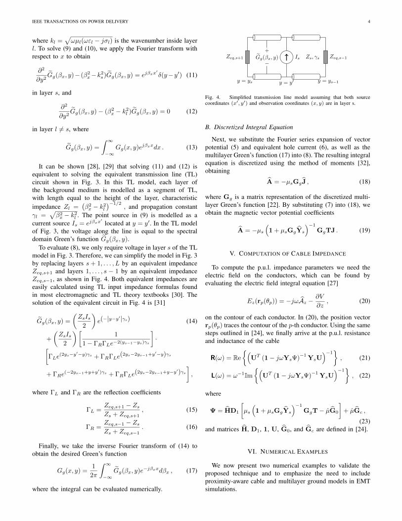
To evaluate (8), we only require voltage in layer s of the TLmodel in Fig. 3. Therefore, we can simplify the model in Fig. 3by replacing layers s + 1, . . . , L by an equivalent impedanceZeq,s+1 and layers 1, . . . , s − 1 by an equivalent impedanceZeq,s−1, as shown in Fig. 4. Both equivalent impedances areeasily calculated using TL input impedance formulas foundin most electromagnetic and TL theory textbooks [30]. Thesolution of the equivalent circuit in Fig. 4 is [31]

Gg(βx, y) =

(ZsIs

2

)e(−|y−y

′|γs) (14)

+

(ZsIs

2

)[1

1− ΓRΓLe−2(ys−1−ys)γs

]·[

ΓLe(2ys−y′−y)γs + ΓRΓLe

(2ys−2ys−1+y′−y)γs

+ ΓRe(−2ys−1+y+y

′)γs + ΓRΓLe(2ys−2ys−1+y−y′)γs

],

where ΓL and ΓR are the reflection coefficients

ΓL =Zeq,s+1 − ZsZs + Zeq,s+1

, (15)

ΓR =Zeq,s−1 − ZsZs + Zeq,s−1

. (16)

Finally, we take the inverse Fourier transform of (14) toobtain the desired Green’s function

Gg(x, y) =1

2π

∫ ∞−∞

Gg(βx, y)e−jβxxdβx , (17)

where the integral can be evaluated numerically.

Zeq,s+1 Zeq,s−1

y = ys y = y′ y = ys−1

Zs, γsIsGg(βx, y)

+

−

Fig. 4. Simplified transmission line model assuming that both sourcecoordinates (x′, y′) and observation coordinates (x, y) are in layer s.

B. Discretized Integral Equation

Next, we substitute the Fourier series expansion of vectorpotential (5) and equivalent hole current (6), as well as themultilayer Green’s function (17) into (8). The resulting integralequation is discretized using the method of moments [32],obtaining

A = −µsGgJ , (18)

where Gg is a matrix representation of the discretized multi-layer Green’s function [22]. By substituting (7) into (18), weobtain the magnetic vector potential coefficients

A = −µs(1 + µsGgYs

)−1GgTJ . (19)

V. COMPUTATION OF CABLE IMPEDANCE

To compute the p.u.l. impedance parameters we need theelectric field on the conductors, which can be found byevaluating the electric field integral equation [27]

Ez(rp(θp)) = −jωAz −∂V

∂z, (20)

on the contour of each conductor. In (20), the position vectorrp(θp) traces the contour of the p-th conductor. Using the samesteps outlined in [24], we finally arrive at the p.u.l. resistanceand inductance of the cable

RRR(ω) = Re

(UT (1− jωYsΨ)

−1YsU

)−1, (21)

LLL(ω) = ω−1Im(

UT (1− jωYsΨ)−1

YsU)−1

, (22)

where

Ψ = HD1

[µs

(1 + µsGgYs

)−1GgT− µG0

]+ µGc ,

(23)and matrices H, D1, 1, U, G0, and Gc are defined in [24].

VI. NUMERICAL EXAMPLES

We now present two numerical examples to validate theproposed technique and to emphasize the need to includeproximity-aware cable and multilayer ground models in EMTsimulations.


10 m

1 m

seabed (ε3 = 15 ε0, µ3 = µ0, σ3 = 0.05 S/m)

air (ε0, µ0)

sea (ε2 = 81 ε0, µ2 = µ0, σ2 = 5 S/m)

Fig. 5. Three-core cable used for validation in Sec. VI.

TABLE ITHREE-CORE CABLE OF SEC. VI-A: GEOMETRICAL AND MATERIAL

PARAMETERS

Core radius = 11.6 mm, ρ = 1.7241 · 10−8 Ω · mInsulation t = 15 mm, εr = 2.3

Metallic Sheath t = 0.22 mm, ρ = 2.20 · 10−7 Ω · m,Jacket t = 4 mm, εr = 2.3

Outer Armor t = 8 mm, r = 80 mm, ρ = 2.86 · 10−8 Ω · m.Armor Insulation t = 3 mm, εr = 2.3

100

102

104

106

2

4

6

Frequency [Hz]

Ind

uct

ance

p.u

.l.

[mH

/km

]

100

102

104

106

100

102

104

Frequency [Hz]

Res

ista

nce

p.u

.l.

[Ω/k

m]

Fig. 6. Cable system of Sec. VI-A: zero-sequence inductance (top panel), andresistance (bottom panel) obtained with MoM-SO (), FEM (·), and analyticformulas ( ). Cable screens are left open.

A. Example #1 - Three-Core Cable

1) Cable Geometry and Material Parameters: The firstexample consists of a three-core cable buried under a shallowsea. The cable geometry is shown in Fig. 5. The geometricaland material properties of the cable are listed in Table I[33]. The surrounding medium is modelled using L = 3layers. The top layer models air. The second layer modelsthe sea, with height of 10 m, conductivity σ2 = 5 S/mand electrical permittivity ε2 = 81 ε0, which are typical forsea water [34]. The bottom layer represents a seabed withconductivity σ3 = 0.05 S/m and permittivity ε3 = 15 ε0 [34].Since the conductors inside the cables are touching each other,significant proximity effects between them are expected [35].

100

102

104

106

0.2

0.25

0.3

0.35

0.4

Frequency [Hz]

Indu

ctan

ce p

.u.l

. [m

H/k

m]

100

102

104

106

100

Frequency [Hz]

Res

ista

nce

p.u

.l. [Ω

/km

]

Fig. 7. As in Fig. 6, but when a positive-sequence excitation is applied tothe core conductors.

2) Impedance Validation: We first calculated the 7 × 7impedance matrix of the cable using the proposed MoM-SO approach. In MoM-SO, the discretization parameters Npand N were set to 4. Next, we repeated the computationwith a commercial FEM solver (COMSOL Multiphysics [36]),following the approach presented in [21]. In order to reproduceskin effect adequately, boundary layer elements were used tofinely mesh the conductor edges. In FEM, we also used theinfinite element domain to truncate the surrounding medium. Atotal of 228,538 elements were required in the FEM simulationto mesh the cable and the surrounding medium. Finally,we calculated the impedance of the cable with the analyticformulas (cable constants [5]) that are implemented in mostEMT tools.

In order to facilitate the comparison of the results obtainedwith MoM-SO, FEM, and analytic formulas, we reduced the7 × 7 impedance matrix to a 3 × 3 matrix by assuming thatthe screens and the armor of the cable are open at bothends1, i.e. we assumed that there is zero net current inside thescreens and armor. Figures 6 and 7 show the cable inductanceand resistance obtained with MoM-SO, FEM, and analyticformulas when zero- and positive-sequence excitations areapplied to the core conductors. An excellent agreement be-tween the results obtained with the proposed MoM-SO methodand FEM can be observed. Analytic formulas instead returninaccurate parameters in both cases. In the case of positivesequence excitation (Fig. 7), inaccuracy is mainly attributedto the neglection of proximity effects. In the zero sequencecase (Fig. 6) inaccuracy is due to proximity effects and thelack of an accurate multilayer ground model.

3) Timing Comparison: The simulation times to calculatethe impedance of the cable are summarized in Table II. FEMtook 190 s per frequency to calculate the impedance of thiscable. On the other hand, MoM-SO took just 0.09 s perfrequency to calculate the impedance parameters with the same

1This assumption is made only to simplify the comparison of the cableparameters, and will not be used in the subsequent transient simulations.


TABLE IIEXAMPLE OF SEC. VI-A: CPU TIME REQUIRED TO COMPUTE THE

IMPEDANCE AT ONE FREQUENCY*

Test Case MoM-SO FEM Speed-upThree-layers 0.089 s 190 s 2136 X

*Simulations were run on a system with 16 GB memoryand 3.40 GHz processor.

1 km

Vcore1Vsheath1

+−1 p.u.

2Ω 0 ms

2Ω

Fig. 8. Setup for transient analysis for the example considered in Sec. VI-A4.

0 0.02 0.04 0.06 0.08 0.10

0.5

1

1.5

Time [ms]

Volt

age

[p.u

.]

0 0.02 0.04 0.06 0.08 0.1−0.05

0

0.05

0.1

Time [ms]

Volt

age

[p.u

.]

Fig. 9. Cable System of Sec. VI-A: Core 1 and sheath 1 voltages obtainedwith MoM-SO ( ) and analytic formulas ( ) for the setup shown in Fig. 8.

accuracy.

4) Transient Simulation: Next, we compare the transientwaveform predicted with analytic formulas and MoM-SO. Weconsider the setup in Fig. 8 where a unit step excitation isapplied to the core conductor of the top-right single core cablein Fig. 5. We created two universal line models [4] for the ca-ble. The first model was derived from the impedance obtainedwith MoM-SO, while the second model was derived fromthe impedance calculated with analytic formulas. For bothmodels, shunt admittance was calculated using the formulasfrom [37]. Figure 9 shows the transient voltages Vcore1 andVsheath1 predicted with MoM-SO and analytic formulas. Thesheath voltage predicted with analytic formulas significantlydeviates from the waveforms predicted with MoM-SO, as aresult of the neglection of proximity and multilayer groundeffects. These results show how the proposed method can leadto more accurate transient results with respect to existing EMTtools, which are mostly based on analytic formulas.

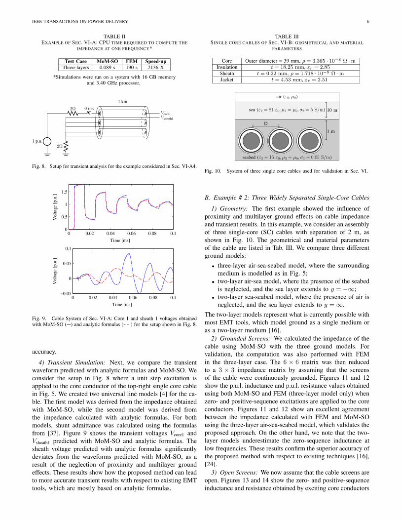
TABLE IIISINGLE CORE CABLES OF SEC. VI-B: GEOMETRICAL AND MATERIAL

PARAMETERS

Core Outer diameter = 39 mm, ρ = 3.365 · 10−8 Ω · mInsulation t = 18.25 mm, εr = 2.85

Sheath t = 0.22 mm, ρ = 1.718 · 10−8 Ω · mJacket t = 4.53 mm, εr = 2.51

10 m

D

1 m

seabed (ε3 = 15 ε0, µ3 = µ0, σ3 = 0.05 S/m)

air (ε0, µ0)

sea (ε2 = 81 ε0, µ2 = µ0, σ2 = 5 S/m)

Fig. 10. System of three single core cables used for validation in Sec. VI.

B. Example # 2: Three Widely Separated Single-Core Cables

1) Geometry: The first example showed the influence ofproximity and multilayer ground effects on cable impedanceand transient results. In this example, we consider an assemblyof three single-core (SC) cables with separation of 2 m, asshown in Fig. 10. The geometrical and material parametersof the cable are listed in Tab. III. We compare three differentground models:• three-layer air-sea-seabed model, where the surrounding

medium is modelled as in Fig. 5;• two-layer air-sea model, where the presence of the seabed

is neglected, and the sea layer extends to y = −∞;• two-layer sea-seabed model, where the presence of air is

neglected, and the sea layer extends to y =∞.The two-layer models represent what is currently possible withmost EMT tools, which model ground as a single medium oras a two-layer medium [16].

2) Grounded Screens: We calculated the impedance of thecable using MoM-SO with the three ground models. Forvalidation, the computation was also performed with FEMin the three-layer case. The 6 × 6 matrix was then reducedto a 3 × 3 impedance matrix by assuming that the screensof the cable were continuously grounded. Figures 11 and 12show the p.u.l. inductance and p.u.l. resistance values obtainedusing both MoM-SO and FEM (three-layer model only) whenzero- and positive-sequence excitations are applied to the coreconductors. Figures 11 and 12 show an excellent agreementbetween the impedance calculated with FEM and MoM-SOusing the three-layer air-sea-seabed model, which validates theproposed approach. On the other hand, we note that the two-layer models underestimate the zero-sequence inductance atlow frequencies. These results confirm the superior accuracy ofthe proposed method with respect to existing techniques [16],[24].

3) Open Screens: We now assume that the cable screens areopen. Figures 13 and 14 show the zero- and positive-sequenceinductance and resistance obtained by exciting core conductors


100

102

104

106

0

2

4

6

Frequency [Hz]

Indu

ctan

ce p

.u.l

. [m

H/k

m]

100

102

104

106

10−1

100

Frequency [Hz]

Res

ista

nce

p.u

.l. [Ω

/km

]

Fig. 11. Cable system of Sec. VI-B: zero-sequence p.u.l. inductance (toppanel) and resistance (bottom panel) obtained with the three-layer air-sea-seabed model in MoM-SO (), three-layer air-sea-seabed model in FEM (·),two-layer air-sea model ( ), and two-layer sea-seabed model ( ). Thescreens are continuously grounded.

100

102

104

106

0

0.5

1

Frequency [Hz]

Ind

uct

ance

p.u

.l.

[mH

/km

]

100

102

104

106

10−1

100

Frequency [Hz]

Res

ista

nce

p.u

.l. [Ω

/km

]

Fig. 12. As in Fig. 11, but when a positive-sequence excitation is appliedto the core conductors.

with zero- and positive-sequence currents. The parametersobtained with MoM-SO match very well the reference FEMresults. The two-layer air-sea model produces inadequateresults because at low frequencies the zero-sequence induc-tance is underestimated, and at high frequencies the positive-sequence inductance is underestimated. The two-layer sea-seabed model is more accurate than the air-sea model, but stillunderestimates the zero-sequence inductance at low frequency.It should be noted that the two layer sea-seabed model cannotbe utilized in some EMT tools that require the conductivity ofthe top layer to be zero.

4) Timing Comparison: In MoM-SO, discretization pa-rameters N and N were set to 4. In FEM, the cable andsurrounding medium were meshed with 255,380 elements.The timing results for both FEM and MoM-SO simulations

100

102

104

106

0

2

4

6

Frequency [Hz]

Indu

ctan

ce p

.u.l

. [m

H/k

m]

100

102

104

106

100

Frequency [Hz]

Res

ista

nce

p.u

.l. [Ω

/km

]

Fig. 13. Cable system of Sec. VI-B: zero-sequence inductance (top panel),and resistance (bottom panel) obtained with the three-layer air-sea-seabedmodel in MoM-SO (), three-layer air-sea-seabed model in FEM (·), two-layer air-sea model ( ), and two-layer sea-seabed model ( ). Cablescreens are left open.

100

102

104

106

0.4

0.6

0.8

1

Frequency [Hz]

Ind

uct

ance

p.u

.l.

[mH

/km

]

100

102

104

106

10−5

100

105

Frequency [Hz]

Res

ista

nce

p.u

.l.

[Ω/k

m]

Fig. 14. As in Fig. 13, but when a positive-sequence excitation is appliedto the core conductors.

TABLE IVEXAMPLE OF SEC. VI-B: CPU TIME REQUIRED TO COMPUTE THE

IMPEDANCE AT ONE FREQUENCY*

Test Case MoM-SO FEM Speed-upThree-layers 0.108 s 179 s 1661 X

*Simulations were run on a system with 16 GB memoryand 3.40 GHz processor.

are summarized in Table IV. MoM-SO takes only 0.1 s perfrequency, and is 1661 times faster than FEM, which requiresalmost three minutes per frequency.

5) Transient Simulation: We now consider the transientresponse of the cable when there is a phase-to-ground faultat the receiving end of the cable as shown in Fig. 15. Thisexample is adopted from [38]. The top panel of Fig. 16 showsthe fault current Ifault in Fig. 15 predicted with the air-sea,


2 km

Vs R1 R1R2

0 ms Ifault

Fig. 15. Setup for transient analysis for the example considered inSec. VI-B5. Voltage source is Vs = 169kV, R1 = 10Ω, and R2 = 100Ω.

0 5 10 15 20 25 30 35

−100

0

100

200

Cu

rrent

[kA

]

Time [ms]

0 5 10 15 20 25 30 350

5

10

Err

or

%

Time [ms]

Fig. 16. Top panel: fault current Ifault computed for the configuration inFig. 15 using the following ground models: three-layer air-sea-seabed model( ), two-layer air-sea model ( ), and two-layer sea-seabed model ( · ).Bottom panel: error between the two-layer models and the three-layer model.

the air-sea-seabed, and the sea-seabed model. The bottompanel of Fig. 16 shows the relative error between the two-layer models and the three-layer model, which is taken asgold standard. Error exceeds 10% when the air-sea model isused, and reaches 8% if the sea-seabed model is used. Whichtwo-layer model provides the most accurate results cannot beestablished a priori, as it depends on how and where the cableis installed. When using such models, an EMT engineer mustthus decide on a case-by-case basis which model should beused. With MoM-SO, this dilemma is avoided, and accuratecable parameters can be obtained in less than a second for allconfigurations. These improvements make cable modeling aneasier and less-error prone task, accessible to a wider audienceof power engineers.

VII. CONCLUSION

A multilayer ground model was proposed for the MoM-SOapproach for cable impedance calculation. With the proposedmodel, the non-uniformity of the medium which surroundssubmarine and underground cables can be accurately takeninto account. Numerical results show that the proposed methodleads to better transient predictions than analytic formulascurrently used in most electromagnetic transient simulators.While the level of achievable accuracy is comparable to afinite elements analysis, MoM-SO is more than 1000 times

faster than finite elements. Moreover, it is simpler to use, sinceit is fully automated and avoids meshing-related issues. Webelieve that these improvements make accurate cable modelinga simpler task for both transients experts as well as powerengineers in general.

VIII. ACKNOWLEDGEMENT

Authors thank Dr. Bjørn Gustavsen (SINTEF Energy Re-search, Norway) for providing the test cases in Sec. VI.

REFERENCES

[1] A. Ametani, N. Nagaoka, Y. Baba, T. Ohno, Power System Transients:Theory and Applications. Boca Raton, FL: CRC Press, 2013.

[2] J. R. Marti, “Accurate modelling of frequency-dependent transmissionlines in electromagnetic transient simulations,” IEEE Trans. Power App.Syst., no. 1, pp. 147–157, 1982.

[3] T. Noda, N. Nagaoka and A. Ametani, “Phase domain modeling offrequency-dependent transmission lines by means of an ARMA model,”IEEE Trans. Power Del., vol. 11, no. 1, pp. 401–411, 1996.

[4] A. Morched, B. Gustavsen, M. Tartibi, “A universal model for accuratecalculation of electromagnetic transients on overhead lines and under-ground cables,” IEEE Trans. Power Del., vol. 14, no. 3, pp. 1032–1038,1999.

[5] A. Ametani, “A general formulation of impedance and admittance ofcables,” IEEE Trans. Power App. Syst., no. 3, pp. 902–910, 1980.

[6] L.M. Wedephol, and D.J. Wilcox, “Transient analysis of undergroundpower-transmission systems. System-model and wave-propagation char-acteristics,” Proc. IEEE, vol. 120, no. 2, pp. 253–260, Feb. 1973.

[7] Filipe Faria da Silva and Claus Leth Bak, Electromagnetic Transientsin Power Cables. Springer, 2013.

[8] J. Weiss, Z.J. Csendes, “A one-step finite element method for multicon-ductor skin effect problems,” IEEE Trans. Power App. Syst., no. 10, pp.3796–3803, 1982.

[9] S. Cristina and M. Feliziani, “A finite element technique for multicon-ductor cable parameters calculation,” IEEE Trans. Magn., vol. 25, no. 4,pp. 2986–2988, 1989.

[10] B. Gustavsen, A. Bruaset, J. Bremnes, and A. Hassel, “A finite elementapproach for calculating electrical parameters of umbilical cables,” IEEETrans. Power Del., vol. 24, no. 4, pp. 2375–2384, Oct. 2009.

[11] S. Habib and B. Kordi, “Calculation of Multiconductor UndergroundCables High-Frequency Per-Unit-Length Parameters Using Electromag-netic Modal Analysis,” IEEE Trans. Power Del., pp. 276–284, 2013.

[12] A. Ametani and K. Fuse, “Approximate method for calculating theimpedances of multiconductors with cross section of arbitrary shapes,”Elect. Eng. Jpn., vol. 112, no. 2, 1992.

[13] E. Comellini, A. Invernizzi, G. Manzoni., “A computer program fordetermining electrical resistance and reactance of any transmission line,”IEEE Trans. Power App. Syst., no. 1, pp. 308–314, 1973.

[14] P. de Arizon and H. W. Dommel, “Computation of cable impedancesbased on subdivision of conductors,” IEEE Trans. Power Del., vol. 2,no. 1, pp. 21–27, 1987.

[15] A. Pagnetti, A. Xemard, F. Paladian and C. A. Nucci, “An improvedmethod for the calculation of the internal impedances of solid and hollowconductors with the inclusion of proximity effect,” IEEE Trans. PowerDel., vol. 27, no. 4, pp. 2063 –2072, Oct. 2012.

[16] O. Saad, G. Gaba, and M. Giroux, “A closed-form approximation forground return impedance of underground cables,” IEEE Trans. PowerDel., vol. 3, pp. 1536–1545, 1996.

[17] F. Pollaczek, “On the field produced by an infinitely long wire carryingalternating current,” Elektrische Nachrichtentechnik, vol. 3, pp. 339–359,1926.

[18] D. A. Tsiamitros, G. K. Papagiannis, and P. S. Dokopoulos, “EarthReturn Impedances of Conductor Arrangements in Multilayer Soils PartI: Theoretical Model,” IEEE Trans. Power Del., vol. 23, no. 4, pp. 2392–2400, Oct 2008.

[19] D. Tsiamitros, G. Papagiannis, and P. Dokopoulos, “Earth returnimpedances of conductor arrangements in multilayer soils–part ii: Nu-merical results,” Power Delivery, IEEE Transactions on, vol. 23, no. 4,pp. 2401–2408, Oct 2008.

[20] T. A. Papadopoulos, G. K. Papagiannis, and D. P. Labridis, “A gen-eralized model for the calculation of the impedances and admittancesof overhead power lines above stratified earth,” Electric Power SystemsResearch, vol. 80, no. 9, pp. 1160–1170, 2010.


[21] Y. Yin and H. W. Dommel, “Calculation of frequency-dependentimpedances of underground power cables with finite element method,”IEEE Trans. Magn., vol. 25, no. 4, pp. 3025–3027, 1989.

[22] U. R. Patel, B. Gustavsen, and P. Triverio, “An Equivalent SurfaceCurrent Approach for the Computation of the Series Impedance of PowerCables with Inclusion of Skin and Proximity Effects,” IEEE Trans.Power Del., vol. 28, pp. 2474–2482, 2013.

[23] ——, “Proximity-Aware Calculation of Cable Series Impedance forSystems of Solid and Hollow Conductors,” IEEE Trans. Power Delivery,vol. 29, no. 5, pp. 2101–2109, Oct. 2014.

[24] U. R. Patel and P. Triverio, “MoM-SO: a Complete Method for Com-puting the Impedance of Cable Systems Including Skin, Proximity, andGround Return Effects,” IEEE Trans. Power Del., 2015, (in press).

[25] D. De Zutter, and L. Knockaert, “Skin Effect Modeling Based on aDifferential Surface Admittance Operator,” IEEE Trans. Microw. TheoryTech., vol. 53, no. 8, pp. 2526 – 2538, Aug. 2005.

[26] U. R. Patel, B. Gustavsen, and P. Triverio, “Application of the MoM-SO Method for Accurate Impedance Calculation of Single-Core CablesEnclosed by a Conducting Pipe,” in 10th International Conference onPower Systems Transients (IPST 2013), Vancouver, Canada, July 18–202013.

[27] C. Balanis, Antenna Theory: Analysis and Design, 3rd ed. Wiley, 2005.[28] N. Fache, F. Olyslager, and D. De Zutter, Electromagnetic and circuit

modelling of multiconductor transmission lines. Clarendon Press, 1993.[29] K. A. Michalski and J. R. Mosig, “Multilayered media Green’s functions

in integral equation formulations,” IEEE Trans. Antennas Propag.,vol. 45, pp. 508–519, 1997.

[30] D. K. Cheng, Field and Wave Electromagnetics (2nd Edition). PrenticeHall, 1989.

[31] F. M. Tesche and T. Karlsson, EMC analysis methods and computationalmodels. John Wiley & Sons, 1997.

[32] R. Harrington, Time-Harmonic Electromagnetic Fields. McGraw-Hill,1961.

[33] ABB, “XLPE Submarine Cable Systems,” ABB Group, Tech. Rep.,2014. [Online]. Available: www.abb.com

[34] A. Martinez and A. P. Byrnes, “Modeling dielectric-constant values ofgeologic materials: An aid to ground-penetrating radar data collectionand interpretation,” Bulletin of the Kansas Geological Survey, p. 16,2001.

[35] U. R. Patel and P. Triverio, “A Comprehensive Study on the Influenceof Proximity Effects on Electromagnetic Transients in Power Cables,”in 11th International Conference on Power Systems Transients (IPST2015), Cavtat, Croatia, 2015.

[36] COMSOL Multiphysics. COMSOL, Inc. [Online]. Available:https://www.comsol.com/

[37] J. Martinez-Velasco, Power System Transients. Parameter Determina-tion. CRC Press, 2010.

[38] T.-C. Yu and J. R. Martı, “A robust phase-coordinates frequency-dependent underground cable model (zcable) for the emtp,” IEEE Trans.Power Del., vol. 18, no. 1, pp. 189–194, 2003.

Utkarsh R. Patel (S’13) received the B.A.Sc. andM.A.Sc. degrees in Electrical Engineering from theUniversity of Toronto in 2012 and 2014, respec-tively. Currently, He is pursuing the Ph.D. degree inElectrical Engineering at the same institution. Hisresearch interests are applied electromagnetics andsignal processing.

Piero Triverio (S’06 – M’09) received the M.Sc.and Ph.D. degrees in Electronic Engineering fromPolitecnico di Torino, Italy in 2005 and 2009, re-spectively. He is an Assistant Professor with theDepartment of Electrical and Computer Engineeringat the University of Toronto, where he holds theCanada Research Chair in Modeling of ElectricalInterconnects. His research interests include signalintegrity, electromagnetic compatibility, and modelorder reduction. He received several internationalawards, including the 2007 Best Paper Award of the

IEEE Transactions on Advanced Packaging, the EuMIC Young Engineer Prizeat the 13th European Microwave Week, and the Best Paper Award at the IEEE17th Topical Meeting on Electrical Performance of Electronic Packaging.

ieee transactions on power delivery 1 … transactions on power delivery 1 accurate impedance...

Documents