ieee transactions on geoscience and remote · pdf fileieee transactions on geoscience and...
TRANSCRIPT
IEEE TRANSACTIONS ON GEOSCIENCE AND REMOTE SENSING, VOL. X, NO. X, AUGUST 2016 1
Forest Change Detection in Incomplete SatelliteImages with Deep Neural Networks
Salman H Khan, Xuming He, Fatih Porikli, and Mohammed Bennamoun
Abstract—Land cover change monitoring is an important taskfrom the perspective of regional resource monitoring, disastermanagement, land development and environmental planning.In this study, we analyze imagery data from remote sensingsatellites to detect forest cover changes over a period of 29years (1987−2015). Since the original data is severely incompleteand contaminated with artifacts, we first devise a spatiotemporalinpainting mechanism to recover the missing surface reflectanceinformation. The spatial filling process makes use of the availabledata of the nearby temporal instances followed by a sparseencoding based reconstruction. We formulate the change detec-tion task as a region classification problem. We build a multi-resolution profile of the target area and generate a candidate setof bounding box proposals that enclose potential change regions.In contrast to existing methods that use handcrafted features,we automatically learn region representations using a deepneural network in a data-driven fashion. Based on these highlydiscriminative representations, we determine forest changes andpredict their onset and offset timings by labeling the candidateset of proposals. Our approach achieves state-of-the-art averagepatch classification rate of 91.6% (an improvement of ∼ 16%)and mean onset/offset prediction error of 4.9 months (an errorreduction of 5.0 months) compared to a strong baseline. We alsoqualitatively analyze the detected changes in the unlabeled imageregions, which demonstrate that the proposed forest changedetection approach is scalable to new regions.
Index Terms—Change detection, Multi-temporal spectral data,Remote sensing, Deep learning, Image inpainting.
I. INTRODUCTION
Ecosystem management and socioeconomic studies at re-gional, national and international scale require the detectionand monitoring of land cover changes. In particular, for-est change detection is crucial for continuous environmen-tal monitoring to closely investigate pressing environmentalissues such as natural resource depletion, biodiversity lossand deforestation. Change detection can also provide essentialinformation to help in disaster management, policy making,area planning and efficient land management. In Australiaalone, forests occupy 125 million hectares, which correspondsto 16% of the total continent’s land and nearly 3% of the totalforest area in the world. Forests are regularly disturbed bysignificant changes, e.g., during 2006-07 to 2010-11, an areaof approximately 39 million hectares was destroyed by fires
S. H. Khan is with the Data61-CSIRO and the Australian National Univer-sity (ANU), Canberra ACT 0200, Australia. Email:[email protected]
X. He is with the ShanghaiTech University, Pudong Xinqu, ShanghaiShi, China. This work was performed when he was with Data61/ANU.Email:[email protected]
F. Porikli is with the Australian National University, Canberra ACT 0200,Australia. Email:[email protected]
M. Bennamoun is with the University of Western Australia, Crawley WA6009, Australia. Email:[email protected]
and 9 thousand hectares were yearly harvested in Australia[1]. These disturbances need to be frequently monitored andanalyzed to develop competent response procedures for forestecosystems.
Current studies using medium spatial resolution satelliteimagery usually perform a synoptic analysis over a tem-poral scale of one or more years [2–5]. The traditionallyused Landsat imagery based systems work at a longer timescale due to their low coverage across the globe and lowrepeat frequency in contrast to the coarse spatial resolutionsatellite imagery sources e.g., Moderate-Resolution ImagingSpectrometer (MODIS), National Oceanic and AtmosphericAdministration (NOAA), and Advanced Very High ResolutionRadiometer (AVHRR). Moreover, climate and weather condi-tions (e.g., continuous cloud cover) significantly restrict theacquisition of quality land cover data.
In this work, we introduce an automatic solution for forestmonitoring at a sub-annual level for applications that requirea more frequent analysis, including grazing land management,crops safety examinations, and natural hazard analysis. Oursolution is also applicable to regions undergoing a rapid forestregeneration (thus requiring a more frequent analysis) to avoidexcessive omission error [6]. We utilize the publicly accessibleLandsat data and monitor changes at a much finer timescale of2 months as opposed to several years. The primary challenge,however, is the severe missing data problem in the Landsatimagery due to limited camera aperture, cloud occlusion andsensor artifacts. To address this issue, we propose a two-stagestrategy for the fine-grain change detection task (see Fig. 1).In the first stage, we take a data-driven approach to fill in themissing spatial data and achieve higher temporal resolutionfrom the available Landsat spectral data sequences (Sec. IV).Our technique is based on image inpainting using sparseencoding. The key idea here is to exploit the temporal andspatial continuity of the underlying events and use statistics ofthe observed image patches to fill in small gaps (Sec. IV-A,IV-B). The resulting high temporal resolution image sequencesenable us to analyze data at a much finer temporal scale.
After obtaining the inpainted time-lapse satellite imagery,we tackle the change detection problem in the second stage.We focus on two sub-problems under the scope of changedetection. The first is the detection of multiple classes andinstances of change events in a specified region. The secondis the estimation of the start and end time of the detectedchange event. For this purpose, we consider the unconstrainedchange discovery in a large geographic area by selecting class-independent change event candidate regions, and predicting thelikelihood of certain change event types along-with their start

IEEE TRANSACTIONS ON GEOSCIENCE AND REMOTE SENSING, VOL. X, NO. X, AUGUST 2016 2
Raw
Tim
e-se
ries
Sate
llit
e Im
ager
y Data Recovery
(Sec. IV)Change Detection
(Sec. V)
Image Gap filling
Recovery via Masked Sparse Reconstruction
Candidate Change Regions Prediction
Proposal Refinement
Deep Neural Net for Automatic Feature
Learning (temporal+spatial)
Multi-resolution Area Profile Generation
Thin Cloud Removal
Fig. 1: An overview of our approach for change detection inincomplete satellite images.
and end times. Our main contributions are threefold:
• In contrast to the existing approaches that rely stronglyon expert’s domain knowledge to extract features, weemploy a deep learning approach to automatically capturethe most appropriate features from the inpainted imagedata at the finer temporal scale (Sec. V). Such deepneural network based approaches have shown superiorperformance in most computer vision tasks such as clas-sification, detection, and segmentation [7–10], and areparticularly suitable for representing signals and theirspatiotemporal context.
• Unlike the traditional pixel-based local change detectiontechniques [11–14], our method incorporates contextualinformation in the form of spatial, spectral and temporalrelationships in a novel deep convolutional neural net-work (CNN) model (Sec. V-C). Thus, our method canbe categorized among the object-based change detectionmethods that are more robust than their pixel-basedcounterparts [15].
• Conventional object-based change detection methodsheavily rely on image segmentation, which often leads toover (excessively large regions) and under (incorrectly toosmall) partitioning of change areas [4, 16]. To alleviatethis problem, we generate change box proposals andselect a candidate set with the help of multi-resolutionarea profiles (Sec.V-A,V-B).
As a case-study, we analyze time-series satellite imageryof the north-east region of Melbourne, Victoria, Australia(Sec. III). Our region-of-interest is a rectangular section withan area of 20,016.1 km2 (7,728.2 mi2) lying between alatitude and longitude of 36000′00.0”S 146000′00.0”E and38000′00.0”S 147000′00.0”E. We detect potential change re-gions in this area and predict their onset and offset timings.Since annotations are available for only a few selected changeregions, we perform both a quantitative and qualitative analysisto assess the performance of our approach on both labeledand unlabeled patches, respectively. Through extensive exper-iments, we show that our approach outperforms all baselinetechniques by a significant margin. Our method attains a mean-IOU score of 84.9% and an average recall rate of 77.7% for thetemporal change detection and patch-wise classification tasks.
In terms of the start and end time predictions for detectedchange events, our method predicts the onset and offset timeswith an average error margin of ∼3 months and ∼6 months,respectively. This performance is remarkably better than thecurrent state-of-the-art approaches, which yield error marginsin years scale (Sec. VI-D).
The rest of the paper is organized as follows. We discussrelated literature in the next section (Sec. II). Data descriptionis provided in Sec. III and data recovery approach is detailedin Sec. IV. Next, we explain our change detection approach inSec. V. The experimental results are reported in Sec. VI andthe paper finally concludes in Sec. VII.
II. RELATED WORK
The prevalent approaches for change detection in remotelysensed data can be categorized into two major classes; low-level local approaches and object-based approaches [4]. Thelow-level approaches use statistical indices derived from thepixel values of spectral images [17]. They are limited topixel-level analysis, thus they remain agnostic to the valuablecontextual information. A conventional approach to pixel-levelchange detection directly compares the contrast of bi-temporal(pair of) images acquired at selected dates when high-qualitydata was available [18]. Similarly, [11] extracts spectral indicesto compare and detect changes in a pair of images. To studyseasonal trends in multiple images, the temporal trajectories ofcoarse to moderate spatial-resolution spectral data have alsobeen analyzed [12]. [19] proposed a pixel-level forest trendindex and studied its performance on the Australian continentLandsat imagery. Compared to our approach, they performanalysis at a much coarse temporal scale (only 10 imagesduring 1989-2006) and work on clean data acquired duringdry seasons.
Other pixel-level change detection techniques use a vege-tation index [20, 21], change vectors [22], spectral mixtureanalysis [23] and local texture [13]. Machine learning basedclassifiers such as Multi-layer Perceptron [24], Decision Trees[25] and Support Vector Machine (SVM) [14] have also beenused for pixel-level change detection. However, these methodsmainly use handcrafted features based on domain expertise.
The object-based approaches consider the contextual infor-mation by working on the homogeneous pixels, which areusually grouped together based on their appearance (spectralinformation), location and/or temporal properties [15]. One ofthe earliest work in object based change detection also uses thegeometrical information of urban structures for object basedanalysis [26]. In most cases, standard unsupervised segmenta-tion and grouping procedures are used to generate such pixelclusters [27]. Since these approaches work on region or objectlevel, they are less prone to spectral variability, geo-referencingeffects and errors in detecting land cover changes comparedto pixel-level approaches [4]. Some object based approaches[13, 28] directly compare objects from different images toaccount for changes. In contrast, the approaches from [29]and [30] compare the extracted objects for change detectiononly after they are categorized into one of the desired classes.
One problem with object-based methods is that they heavilydepend on the segmentation methods used for the generation

IEEE TRANSACTIONS ON GEOSCIENCE AND REMOTE SENSING, VOL. X, NO. X, AUGUST 2016 3
20 km 20 km
Db-37: [370S,1460E]-[380S,1470E] Db-36: [360S,1460E]-[370S,1470E]
Fig. 2: The two study regions (left and right) for change detection are forests in Victoria, Australia (courtesy of Google Maps).
of objects [15, 31]. Not all objects generated in this manner areof the same size, and therefore over and under segmentationerrors lead to less accurate change detection results [4]. Toavoid such errors, we propose to generate bounding boxcandidates at multiple scales to detect interesting changesof varying sizes. Moreover, existing works use hand-craftedfeatures or spectral indices derived from the objects for changemonitoring [18, 31]. In contrast, this work automatically learnsuseful feature representations and predicts change likelihoodsusing a deep neural network.
Spectral remote sensing data suffers from several artifactsand various approaches have been proposed in the literature forpreprocessing and data recovery [32, 33]. The preprocessingtechniques deals with problems such as image registrationfor mosaic generation and the radiometric, atmospheric andtopographic corrections needed to improve raw spectral data[34, 35]. From the perspective of frequent change analysis,a more crucial issue is the recovery of data missed due tosensor errors, seasonal and weather conditions. Data recoveryapproaches normally use image inpainting, multi-spectral andmulti-temporal information [36].
Image inpainting approaches (e.g., [37, 38]) give visuallypleasing results, however they fail to recover very large regionsof missing data and the recovered information is not reliablefor change analysis. Multi-spectral approaches (e.g., [39, 40])use spectral information from other bands or sensors (e.g.,MODIS in [41]) to estimate missing information in the LandsatETM+ (Enhanced Thematic Mapper Plus) images. However,the spectral bands from other sensors suffer from differencesin spatial resolution and bandwidths. The method in [42],called Automated Cloud Cover Assessment (ACCA), uses thereflective and thermal properties of the captured image for
cloud cover estimation. This technique fails for the case of thincirrus clouds (present at higher altitudes) because of their weakthermal signature. Compared to ACCA, Function of Mask(Fmask) [31] method for cloud and their shadow detectionperforms slightly better but still misses very thin cirrus clouds.Two types of auxiliary images are used by [33] to combinethe high-frequency and the low-frequency information for datarecovery.
Our approach for data recovery lies under the category ofmulti-temporal imagery based methods. These methods relyon both the temporal and spatial contextual information andwork best for the recovery of large missing regions. Onesuch approach from [32] assumes that land cover changesare insignificant over a short time-duration and use cloud-free patches to recover contaminated data. Similarly, otherapproaches (e.g., [43–45]) present sophisticated methods toperform data recovery across temporal domain by either re-adjusting the patch statistics or directly predicting the inten-sities. In contrast to these approaches, our method performsdata recovery using reliable temporal information and canalso recover regions contaminated by transparent clouds. Fur-thermore, the proposed approach is fairly straightforward anduses multi-resolution profiles which keep the recovered dataconsistent and reliable for valid change analysis.
The combination of complementary information obtainedfrom multiple remote sensors has also been studied in theliterature to remove mutual inconsistensies [46]. This provesto be useful because different data modalities have varyingmeasurement resolutions, failure rates and sensitivity to atmo-spheric conditions (e.g., cloud cover). Shen et. al[47] fusedhigh frequency and high spatial-resolution data streams toleverage the benefits of both for surface urban heat island anal-

IEEE TRANSACTIONS ON GEOSCIENCE AND REMOTE SENSING, VOL. X, NO. X, AUGUST 2016 4
Feb‐99 Nov‐01 Aug‐04 Apr‐07 Jan‐10 Oct‐12 Jul‐15
1
3
5
7
9
11
13
15
17
19
21
23
25
27
29
31
33
35
37
39
41
43
45
47
49
51
53
55
57
59
61
63
65
67
Timeline for the Change EventsChan
ge Regions Iden
tified by the Experts
Fire Incidents Harvest Incidents
Fig. 3: Gantt chart of the fire and harvest incidents in the regions of interest identified during the period 1999-2015. Fireregions are usually recovered in a shorter period compared to the harvest regions.
ysis. Multi-sensory information was jointly used to producebetter estimates of urban growth maps in densely populatedregions [48]. Fablet and Rousseau [49] suggested an inpaintingapproach to benefit from the mutual strengths of microwaveand infrared measurements for sea surface temperature. Apartfrom applications in geophysical analysis, interpolation ofmissing data using multiple data sources has also been used inbiophysical monitoring e.g., vegetation mapping [50]. Differ-ent to these approaches, we only consider output from a singleremote sensor to interpolate missing information to enablemore frequent forest cover analysis.
More recently, convolutional neural networks (CNN) havebeen used for object detection and segmentation in remotelysensed multi-spectral images [16]. Penatti et. al [51] found thatdeep features that are extracted from a network pretarined onregular color images, generalize very well to satellite images.Transfer learning paradigm has also been investigated to learnbetter representations from remotely sensed data. Gueguenand Hamid [52] used a CNN model, fine-tuned on a largenumber of satellite images, for damage detection. Multi-scaleconvolutional architectures were also learned to obtain pixel-
level segmentation in satellite images [53]. Among otherapplications, CNN models have been used for high-resolutionremotely-sensed scene classification [54, 55], road networksegmentation [56] and vehicle detection [57]. In contrast tothese techniques, our approach deals with change detection inforest cover and provides a mechanism to extract and combinelocalized feature representations using a CNN.
III. STUDY AREA
We analyzed a 222.4 × 90.0 km2 rectangular area in thenorth-east of Melbourne city in Victoria, Australia (Figure 2).The remote sensing satellite data is provided by the AustralianReflectance Grid (ARG) from the Geoscience Australia (GA).ARG is a medium resolution (0.000250 ∼= 25m) grid ofsurface reflectance data based on United States GeologicalSurvey’s (USGS) Landsat TM/ETM+ imagery. To make thedata comparable, robust physical models of [59, 60] are used toremove the differences caused due to sensor geometry, surfacegeometry, sun and atmospheric characteristics. With each ofthe surface reflectance image, a corresponding map of pixelquality flags is provided. For each grid cell, this map indicates

IEEE TRANSACTIONS ON GEOSCIENCE AND REMOTE SENSING, VOL. X, NO. X, AUGUST 2016 5
Fig. 4: Examples of artifacts in the data. There exist large regions of missing data along with strong clouds and their shadows.SLC-off artifacts are shown in the two right-most images which appear as slanted wedge-shaped regions of missing data (figurebest seen when enlarged). Artifacts constitute almost 75.9% of the data.
the presence or absence of null values, band saturation, cloudsand cloud shadows. The processed reflectance data is referredto as the Landsat Nadir Bidirectional Reflectance DistributionFunction (BRDF)-Adjusted (NBAR) images.
The flags included in the pixel quality map are shownin Table I. Notice that, the two cloud flags are included inthe map based on two different methods. The first clouddetection method used is the ACCA algorithm of [42, 58].The second cloud detection method used is the Fmask algo-rithm proposed by [31]. Fmask utilizes Top of AtmosphereReflectance (TOAR) for cloud detection and performs betterthan the ACCA algorithm. Therefore, in this work, we useclouds detected with the Fmask algorithm during the prepro-cessing phase. It is important to note that very thin clouds arestill missed by both methods and therefore we describe ourapproach to remove such clouds in Sec. IV-C.
The study area is divided into two regions of equal di-mensions. Since the available data of both regions belongsto different time-ranges, we refer to the region betweencoordinates 37000′00.0”S 146000′00.0”E and 38000′00.0”S147000′00.0”E as Db-37 and the region between co-ordinates 36000′00.0”S 146000′00.0”E and 37000′00.0”S147000′00.0”E as Db-36. For Db-37, we have a time lapsesequence between 1999-2015 (17 years) of surface reflectancedata and the corresponding pixel quality maps. For Db-36, we
TABLE I: The flags included in the pixel quality map availablewith the Landsat NBAR images. The remaining bit locationsare not currently used.
Bit Position Flag Purpose
0-4 Respective band 1-5 is saturated5 Band 6-1 is saturated6 Band 6-2 is saturated7 Band 7 is saturated8 Contiguity (No Null Values)9 Land or Sea
10 Clouds (ACCA [42, 58])11 Clouds (Fmask [31])12 Cloud shadows (ACCA)13 Cloud shadows (Fmask)14 Topographic Shadow
have surface reflectance data and pixel quality maps for years1987-2014 (28 years).
The remote sensing data is labeled with two types of forestchanges, namely harvests and fire incidents. During the periodof 17 years in the region Db-37, a total of 99 incidents weremanually identified by experts, out of which 50 were fireincidents while the remaining 49 were harvest incidents. These99 change incidents happened at 68 distinct sites. Similarly,a total of 49 incidents were recorded in Db-36 during the 28years period, out of which 14 were fire incidents while 35were harvest incidents. These change events took place at 29different sites. The Gantt chart representation for both typesof annotations in Db-37 is shown in Figure 3. Note that thefire incidents usually last for a much shorter period (and alsorecover quickly) compared to the harvest incidents.
IV. DATA RECOVERY
The data under investigation contains several artifacts dueto which land cover is not always visible in the ARG (seeexamples in Figure 4). These artifacts include missing sur-face reflectance data, heavy clouds and saturated channels inremotely sensed data. Moreover, black stripes (wedge shapedgaps) appear in the Landsat-7 ETM+ imagery due to the failureof the scan line corrector (SLC) in 2003. There is no temporalrelationship between the missing data locations, i.e., theselocations do not remain consistent at different instances oftime. To illustrate by an example, approximately 40.7% ofthe total reflectance data in the Db-37 is missing while nearly35.2% of the data is cloudy. For land cover change analysisand detection, it is necessary to remove these artifacts, whichmake a staggering ∼75.9% of the reflectance data in Db-37.In the current work, we do not aim to remove light cloudshadows or topographical shadows, which also create visualartifacts but are not as severe as the artifacts described above.
To fill-in the missing data and the residual cloudy regions,we design a three-stage image completion process that exploitsthe redundancy in the raw image data. The first stage dealswith large gaps by assessing the reliability of data alongthe temporal domain (Sec. IV-A). The second stage performsa spatial refinement to remove noisy data and ensure spa-tially consistency (Sec. IV-B). The last stage performs furtherrefinement by removing very thin and transparent clouds
IEEE TRANSACTIONS ON GEOSCIENCE AND REMOTE SENSING, VOL. X, NO. X, AUGUST 2016 6
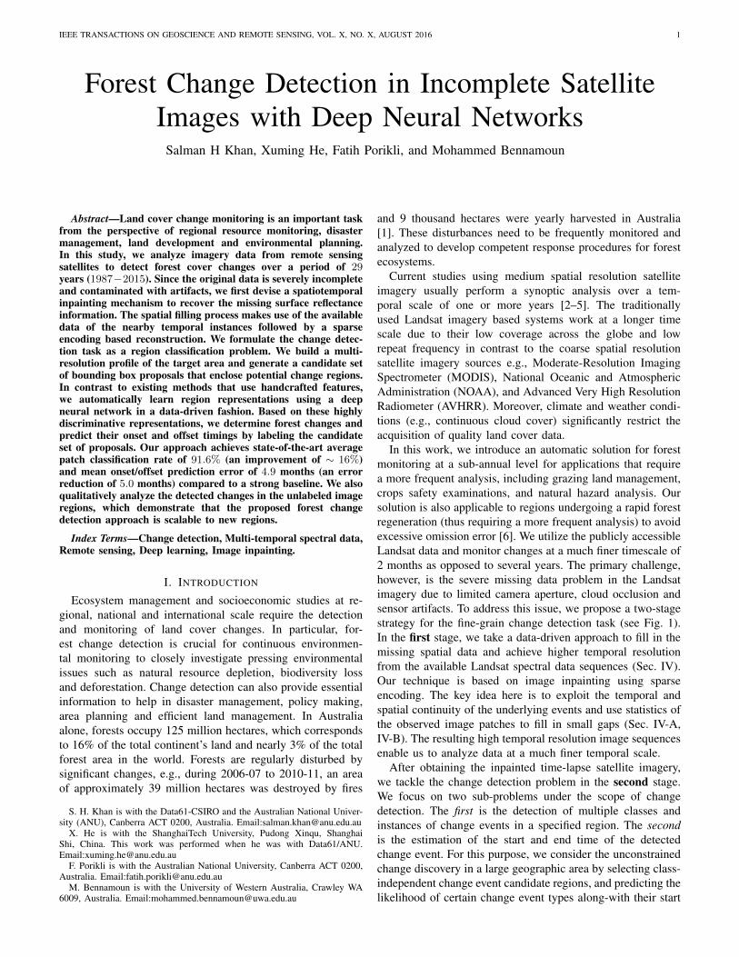
Fig. 5: Data recovery results on single frames: The top row shows raw spectral data, which suffers from several artifactsincluding weather conditions. The bottom row illustrates our recovered images, which are visually more pleasing and moresuitable for further analysis.
(Sec. IV-C). These three stages are elaborated in the followingsections.
A. Gap Filling
In the first stage, we fuse the reliable data along the temporaldimension to generate one representative image for a period ofapproximately two months using the corresponding flags in theavailable pixel quality map. Then, we construct a mean imagefrom the representative images to obtain a yearly backgroundprofile, which we employ consecutively to fill the remainingmissing pixels in the original images. In our experiments, thistemporal strategy yields better performance than pixel-wiseinterpolation that only uses spatial information leading intoadditional artifacts. Since the original satellite images wereacquired at an average frequency of 12 days, this stage canfill in a large percentage of missing pixels without affectingforest change events, which are usually slower processes.
B. Masked Sparse Reconstruction
In the second stage, we further enhance the image framesusing masked sparse reconstruction to enforce the spatialconsistency and remove possible artifacts generated from thefirst stage. We elaborate our approach below.
Given a set of input images {I}1×N , we first extract samesize overlapping patches with dimensions s× s and a uniformstep of p. These patches form a set P = {pi}Mi=1, wherenormally M is a considerably large number. To make thedictionary learning step computationally feasible, we randomlychoose a relatively smaller set of patches denoted by P ={pi}mi=1. Typically, the learned dictionary is composed of r
basis vectors, where r << m1. The objective minimizedduring the dictionary learning process is defined as follows:
minD∈C
1
m
m∑i=1
minαi∈Rr
(1
2‖ pi −Dαi ‖22
)+λ ‖ αi ‖1 +γ ‖ αi ‖22
(1)where, λ and γ are the regularization parameters which enforcea sparse solution for αi. The set C is the constraint set ofmatrices defined as follows:
C = {D ∈ Rq×r s.t., ‖ dj ‖22≤ 1, j ∈ [1, r]}. (2)
The above constraints on the basis vectors (columns of dictio-nary D) avoid arbitrary large values in the learned dictionary.Notice that, we form an over-complete dictionary by settinga small patch size (s), therefore r > s2. The sparse codingproblem posed in Eq. 1 is solved using the online dictionarylearning algorithm of [61].
Once a dictionary has been learned, each image patch pi canbe reconstructed using a sparse combination of basis vectorsin D. However, as discussed in Sec. IV, the spectral data hassevere artifacts and it is quite possible that some of the regionsare still not fully recovered during the first-stage inpaintingprocedure. If we perform a normal reconstruction step using allthe pixels in a given patch, it will lead to errors because someof the patch information may not be valid (appearing usuallyas black regions). Therefore, during the sparse reconstructionstep, we only reconstruct the valid regions (original valid dataand the recovered regions in the inpainting step in Sec. IV-A)
1In our experiments, the following parameter settings were used: s =8, p = 2,m = 5 × 10⁵ and r = 512. The total number of patches (M )were ∼ 2.0× 10⁹ and ∼ 3.8× 10⁹ for Db-37 and Db-36 respectively.
IEEE TRANSACTIONS ON GEOSCIENCE AND REMOTE SENSING, VOL. X, NO. X, AUGUST 2016 7
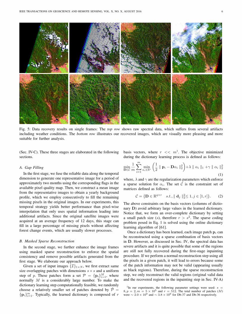
Fig. 6: Left: Gap filling output, Right: The masked sparse re-construction step reduces noise and removes boundary effectscaused by the gap filling.
and do not include the missing pixels in the approximationprocess (Eq. 3). This step fills in small regions of missingdata and removes abrupt changes in pixel contrast since thedictionary D is constructed from only clean patches. Theobjective function for this recovery step can be formulatedas follows:
minαi∈Rr
1
2‖Mi(xi −Dαi) ‖22 +λ′ ‖ αi ‖0, ∀i ∈ [1,M ],
(3)where, λ′ is a regularization parameter to enforce sparsity,Mi ∈ R is a mask defined as a diagonal matrix: Mi =diag(βi) and βi ∈ {0, 1}s
2×1. The mask Mi encodes thevalidity of each pixel. More precisely, the pixels that are notrecovered during the first stage of recovery process are markedas invalid pixels.
The optimization problem in Eq. 3 is solved using theorthogonal matching pursuit (OMP) algorithm [62]. A finalcomplete image is obtained by combining all the small patchespi and performing an averaging operation over overlappedregions. Finally, note that the sparse reconstruction step isperformed individually for each channel of the reflectance databy learning a separate dictionary. This preserves the distinctinformation in each spectral band and ensures a consistentrecovery of the missing information. The improvement isillustrated via an example in Fig. 6.
C. Thin Cloud Removal
The third stage of our data recovery addresses the residualthin clouds in the recovered images. At this stage, all themissing data regions are filled-in, however, some partially-missing regions can still occur due to the thin clouds. Notethat, state-of-the-art cloud detection methods (ACCA andFmask) fail to find thin layers of clouds. Besides, the pixelquality map (Sec. III) does not indicate their location. Thesetranslucent regions cause problems during the later stages ofchange detection (e.g., region proposal generation). Therefore,we devise an efficient approach based on color heuristics toremove the thin clouds (Figure 7).
In the forest region under consideration, thin clouds appearin the Band 1 of the surface reflectance data (blue pixels inFigure 4). More importantly, these thin clouds appear anddisappear abruptly and do not occupy one spatial location
Time-lapse
Sequence of
Images
Yearly Profile
Overall
Background
Profile
Year 1Year 2Year N
Information
Flow for Cloud
Removal
Cloud
Detection
using
Generated
Profile
Cloud
Detection
using
Generated
Profile
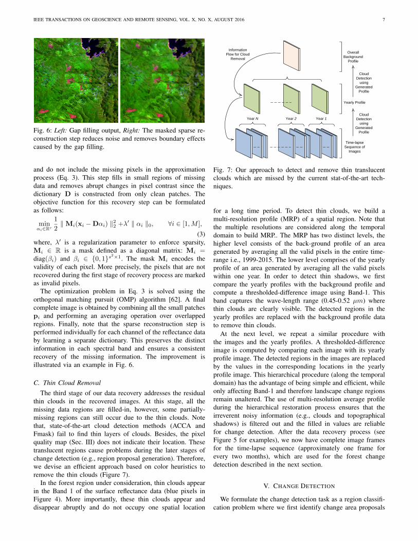
Fig. 7: Our approach to detect and remove thin translucentclouds which are missed by the current stat-of-the-art tech-niques.
for a long time period. To detect thin clouds, we build amulti-resolution profile (MRP) of a spatial region. Note thatthe multiple resolutions are considered along the temporaldomain to build MRP.. The MRP has two distinct levels, thehigher level consists of the back-ground profile of an areagenerated by averaging all the valid pixels in the entire time-range i.e., 1999-2015. The lower level comprises of the yearlyprofile of an area generated by averaging all the valid pixelswithin one year. In order to detect thin shadows, we firstcompare the yearly profiles with the background profile andcompute a thresholded-difference image using Band-1. Thisband captures the wave-length range (0.45-0.52 µm) wherethin clouds are clearly visible. The detected regions in theyearly profiles are replaced with the background profile datato remove thin clouds.
At the next level, we repeat a similar procedure withthe images and the yearly profiles. A thresholded-differenceimage is computed by comparing each image with its yearlyprofile image. The detected regions in the images are replacedby the values in the corresponding locations in the yearlyprofile image. This hierarchical procedure (along the temporaldomain) has the advantage of being simple and efficient, whileonly affecting Band-1 and therefore landscape change regionsremain unaltered. The use of multi-resolution average profileduring the hierarchical restoration process ensures that theirreverent noisy information (e.g., clouds and topographicalshadows) is filtered out and the filled in values are reliablefor change detection. After the data recovery process (seeFigure 5 for examples), we now have complete image framesfor the time-lapse sequence (approximately one frame forevery two months), which are used for the forest changedetection described in the next section.
V. CHANGE DETECTION
We formulate the change detection task as a region classifi-cation problem where we first identify change area proposals
IEEE TRANSACTIONS ON GEOSCIENCE AND REMOTE SENSING, VOL. X, NO. X, AUGUST 2016 8
H
W
W/4H/4
W/8H/8
H/16 W/16
1
2
3
4
41 2 3
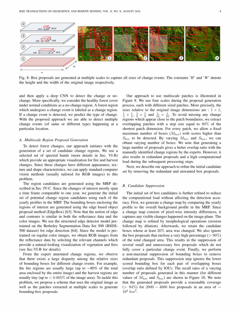
Fig. 8: Box proposals are generated at multiple scales to capture all sizes of change events. The constants ’H’ and ’W’ denotethe height and the width of the original image respectively.
and then apply a deep CNN to detect the change or no-change. More specifically, we consider the healthy forest coverunder normal conditions as a no-change region. A forest regionwhich undergoes a change event is labeled as a change region.If a change event is detected, we predict the type of change.With the proposed approach we are able to detect multiplechange events (of same or different type) happening at aparticular location.
A. Multiscale Region Proposal Generation
To detect forest changes, our approach initiates with thegeneration of a set of candidate change regions. We use aselected set of spectral bands (more details in Sec. VI-B)which provide an appropriate visualization for fire and harvestchanges. Since these changes have different appearance, tex-ture and shape characteristics, we can apply standard computervision methods (usually tailored for RGB images) to thisproblem.
The region candidates are generated using the MRP de-scribed in Sec. IV-C. Since the changes of interest mostly spana time frame comparable to one year, we generate the initialset of potential change region candidates using each of theyearly profiles in the MRP. The bounding boxes enclosing theregions of interest are generated using the edge based objectproposal method (EdgeBox) [63]. Note that the notion of edgeand contours is similar in both the reflectance data and thecolor images. We use the structured edge detector model pre-trained on the Berkeley Segmentation Data Set 500 (BSDS-500 dataset) for edge detection [64]. Since the model is pre-trained on regular color images, we obtain RGB images fromthe reflectance data by selecting the relevant channels whichprovide a natural-looking visualization of vegetation and fires(see Sec.VI-B for details).
From the expert annotated change regions, we observethat there exists a large disparity among the relative sizesof bounding boxes for different change events. For example,the fire regions are usually large (up to ∼80% of the totalarea enclosed by the entire image) and the harvest regions areusually tiny (up to < 0.005% of the image area). To tackle thisproblem, we propose a scheme that uses the original image aswell as the patches extracted at multiple scales to generatebounding-box proposals.
Our approach to use multiscale patches is illustrated inFigure 8. We use four scales during the proposal generationprocess, each with different sized patches. More precisely, thesizes relative to the original image dimensions are : 1 × 1,14 ×
14 , 1
8 ×18 and 1
16 ×116 . To avoid missing any change
regions which appear close to the patch boundaries, we extractoverlapping patches with a step size equal to 80% of theshortest patch dimension. For every patch, we allow a fixedmaximum number of boxes (Mbox) with scores higher thanSbox to be detected. By varying Mbox and Sbox, we canobtain varying number of boxes. We note that generating alarge number of proposals gives a better overlap ratio with themanually identified change regions by the experts. However, italso results in redundant proposals and a high computationalload during the subsequent processing steps.
Next, we describe our approach to refine the initial candidateset by removing the redundant and unwanted box proposals.
B. Candidate Suppression
The initial set of box candidates is further refined to reducethe computational load without affecting the detection accu-racy. First, we generate a change map by comparing the yearlyprofile to the overall background profile in the MRP. Sincea change map consists of pixel-wise intensity differences, itcaptures any visible changes happened on the image plane. Thechange map is refined by morphological operations (erosionfollowed by dilation). Afterwards, we retain the candidateboxes whose at least 20% area was changed. We also ignorethe box proposals that enclose a very high percentage (> 90%)of the total changed area. This results in the suppression ofseveral small and unnecessary box proposals which do notfully cover a particular change event. Finally, we performa non-maximal suppression of bounding boxes to removeredundant proposals. This suppression step ignores the lowerscored bounding box for each pair of overlapping boxes(overlap ratio defined by IOU). The recall rates of a varyingnumber of proposals generated in this manner (for differentvalues of Mbox and Sbox) are shown in Figure 10. We notethat the generated proposals provide a reasonable coverage(> 94%) for 2000 − 4000 box proposals in an area of ∼104 km2.
IEEE TRANSACTIONS ON GEOSCIENCE AND REMOTE SENSING, VOL. X, NO. X, AUGUST 2016 9
3x3x3
(@64)
3x3x3
(@128)
3x3x3
(@256)
3x3x3
(@512)
3x3x3
(@512)
7x7
(@4096)
1x1
(@4096)
(@N
o. o
f C
ha
ng
e C
lasse
s+
1)
F’(i)
Convolution
Layer
Max-pooling
Layer
Fully Connected
Layer
Soft-max
Loss Layer
Data
BlobsKey:
F(i-t)
F(i)
F(i+t)
P(i)
P(i-t)
P(i+t)
Ma
x-p
oo
ling
(alo
ng
th
e te
mp
ora
l
do
ma
in)
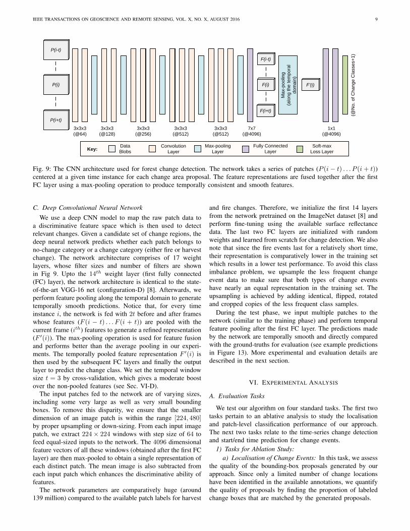
Fig. 9: The CNN architecture used for forest change detection. The network takes a series of patches (P (i − t) . . . P (i + t))centered at a given time instance for each change area proposal. The feature representations are fused together after the firstFC layer using a max-pooling operation to produce temporally consistent and smooth features.
C. Deep Convolutional Neural NetworkWe use a deep CNN model to map the raw patch data to
a discriminative feature space which is then used to detectrelevant changes. Given a candidate set of change regions, thedeep neural network predicts whether each patch belongs tono-change category or a change category (either fire or harvestchange). The network architecture comprises of 17 weightlayers, whose filter sizes and number of filters are shownin Fig 9. Upto the 14th weight layer (first fully connected(FC) layer), the network architecture is identical to the state-of-the-art VGG-16 net (configuration-D) [8]. Afterwards, weperform feature pooling along the temporal domain to generatetemporally smooth predictions. Notice that, for every timeinstance i, the network is fed with 2t before and after frameswhose features (F (i − t) . . . F (i + t)) are pooled with thecurrent frame (ith) features to generate a refined representation(F ′(i)). The max-pooling operation is used for feature fusionand performs better than the average pooling in our experi-ments. The temporally pooled feature representation F ′(i) isthen used by the subsequent FC layers and finally the outputlayer to predict the change class. We set the temporal windowsize t = 3 by cross-validation, which gives a moderate boostover the non-pooled features (see Sec. VI-D).
The input patches fed to the network are of varying sizes,including some very large as well as very small boundingboxes. To remove this disparity, we ensure that the smallerdimension of an image patch is within the range [224, 480]by proper upsampling or down-sizing. From each input imagepatch, we extract 224× 224 windows with step size of 64 tofeed equal-sized inputs to the network. The 4096 dimensionalfeature vectors of all these windows (obtained after the first FClayer) are then max-pooled to obtain a single representation ofeach distinct patch. The mean image is also subtracted fromeach input patch which enhances the discriminative ability offeatures.
The network parameters are comparatively huge (around139 million) compared to the available patch labels for harvest
and fire changes. Therefore, we initialize the first 14 layersfrom the network pretrained on the ImageNet dataset [8] andperform fine-tuning using the available surface reflectancedata. The last two FC layers are initialized with randomweights and learned from scratch for change detection. We alsonote that since the fire events last for a relatively short time,their representation is comparatively lower in the training setwhich results in a lower test performance. To avoid this classimbalance problem, we upsample the less frequent changeevent data to make sure that both types of change eventshave nearly an equal representation in the training set. Theupsampling is achieved by adding identical, flipped, rotatedand cropped copies of the less frequent class samples.
During the test phase, we input multiple patches to thenetwork (similar to the training phase) and perform temporalfeature pooling after the first FC layer. The predictions madeby the network are temporally smooth and directly comparedwith the ground-truths for evaluation (see example predictionsin Figure 13). More experimental and evaluation details aredescribed in the next section.
VI. EXPERIMENTAL ANALYSIS
A. Evaluation Tasks
We test our algorithm on four standard tasks. The first twotasks pertain to an ablative analysis to study the localisationand patch-level classification performance of our approach.The next two tasks relate to the time-series change detectionand start/end time prediction for change events.
1) Tasks for Ablation Study:a) Localisation of Change Events: In this task, we assess
the quality of the bounding-box proposals generated by ourapproach. Since only a limited number of change locationshave been identified in the available annotations, we quantifythe quality of proposals by finding the proportion of labeledchange boxes that are matched by the generated proposals.

IEEE TRANSACTIONS ON GEOSCIENCE AND REMOTE SENSING, VOL. X, NO. X, AUGUST 2016 10
b) Patch-level Change Classification: For this task, wetreat the change detection problem as a classification task.Therefore, for a given time-lapse sequence, we treat eachframe as an independent instance and predict whether or nota change happened in a given frame. For evaluation, we usethe overall accuracy and the recall measure averaged over theclasses.
2) Tasks for Change Detection:a) Time-series Change Detection: For this task, we make
use of the temporal information while making change predic-tions. To enforce a temporal consistency in the predictions, weperform feature fusion in a small window defined over featurescomputed for the same region at adjacent time instances.We also, smooth the output predictions from the baselineapproaches to have a uniform detection pattern. The evaluationmetric used for this case is the average intersection over union(IOU) score obtained over all the labeled change regions.
b) Change On/Offset Prediction: In this task, the onsetand offset of a change event is predicted for a given region.Information across multiple time instances is used to predicta smooth change sequence and to avoid multiple noisy spikesin the prediction. For evaluation, we use the mean taxi-cabdistance for both the onset and offset points of change eventpredictions.
B. Experimental SettingsIn all our results, we report performances on the complete
dataset including both the original and the recovered regions.It is important to note that the recovered regions make a sig-nificant portion of the dataset under investigation and thereforemake the change detection highly challenging. We perform 10fold cross-validation by keeping the train vs. test split to 90%vs. 10%. Mutually exclusive sets of change locations are usedfor training and testing procedures, and care has been takento ensure that an event does not split between the train andthe test set.
We use a combination of bands 5, 4 and 1 from theLandsat 7 imagery and bands 6, 5, and 2 from the Landsat 8imagery for training and testing. These band combinations forLandsat 7 and 8 are suitable for natural-looking visualizationof vegetation and fires (see Figures 5, 14 and 15). The healthy,dry and sparse vegetation appears in bright green, orange andbrown colors respectively. Grasslands appear in light greencolor while water is usually blue. The fire regions appearin dark red color. Since these band combinations provide anatural looking visualization of forest cover, we can applystandard computer vision algorithms and pre-trained modelson the spectral data.
To enhance the contrast of the image, we perform a uniformrescaling of the red, green and blue channels within theranges of 0.0055-0.0463, 0.0132-0.0600 and 0.0029-0.0175,respectively. This helps in the feature extraction process andthe uniform mapping ensures that multiple frames remaincomparable to each other for multi-temporal analysis.
C. Baseline ApproachesWe compare our approach with strong baselines which
use popular handcrafted features and strong machine learning
classifiers. These baselines are described next.1) Handcrafted Features for Classification: We use dense
Scale Invariant Feature Transform (SIFT) descriptors as abaseline for change detection. Based on these features, weexperiment with three classifiers: i) linear support vectormachine (SVM) for max-margin classification, ii) kernel SVMfor nonlinear classification, and iii) random forest (RF) forensemble learning based classification. For the kernel SVM,we use the efficient homogeneous kernel mapping [65] toapproximate the χ2 kernel. The SIFT descriptors are computedon a dense grid and the classifier is directly trained on theselocal features. Note that this was feasible because the pixellabelling of the change regions is known within each patch.During the testing phase, we classify a given image patchas a change region if at least 15% of the SIFT descriptorsare classified as the fire or harvest change. This percentagewas set using cross-validation experiments, which providedapproximately equal true-positive and true-negative rates.
2) Bag-of-Visual-Words (BoW) for Classification: For theBoW baseline, we use dense SIFT as local features andefficiently compute a dictionary using the k-means clustering.The number of bins is set to 600 by cross validation. Allthe features are then represented in terms of associations withthe dictionary atoms. A conventional BoW model does notpreserve the spatial information. However, this informationcan be useful to categorize change patterns with distinctiveshapes. Therefore, to incorporate the spatial information, weuse disjoint spatial bins to compute histograms which are thenstacked together to obtain a final representation. Similar to theprevious baseline, we use linear SVM, χ2-kernel SVM, andRF classifier for prediction.
D. Results
1) Ablative Analysis: We first evaluate the performance ofour bounding-box proposal generation scheme on the Db-37region. The varying number of bounding-box proposals affectthe amount of coverage for the labeled change regions. Thetrend is illustrated in Figure 10. We consider a successfulmatch between the ground-truth bounding-box and the gener-ated proposal if their IOU > 0.1. We generate different numberof bounding-box proposals by changing values of the constantsMbox and Sbox. The higher number of box proposals providemore coverage but also require more computational resourcesfor further processing. To make a balanced choice, we setMbox = 30 and Sbox = 0.05 in our experiments to generate∼1900 box proposals, which cover 94% of the labeled changeregions.
We have also experimented with other box proposal gen-eration methods and analyzed their performance comparedto EdgeBox. These box proposal methods include selectivesearch [66], constrained parametric min-cuts (CPMC [67])and objectness measure [68]. The parameters of these modelswere set to generate nearly the same number of boxes asgenerated by the EdgeBox. In the cases where the numberof generated boxes was very large (e.g., objectness measure),we only considered the box proposals with the highest scorefor evaluation. For each of these methods, we recorded the
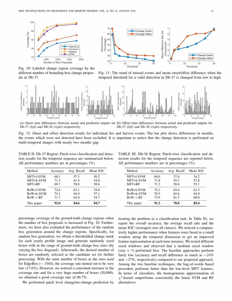
IEEE TRANSACTIONS ON GEOSCIENCE AND REMOTE SENSING, VOL. X, NO. X, AUGUST 2016 11
Number of Box Proposals0 1000 2000 3000 4000
Cov
erag
e (%
)
20
40
60
80
100
ObjectnessSel-SearchEdgeBoxCPMC
Fig. 10: Labeled change region coverage by thedifferent number of bounding-box change propos-als in Db-37.
Threshold0 10 20 30
Mis
sed
Eve
nt
Per
cent
age
10
20
30
40
50
60
70Change OnsetChange Offset
Threshold0 10 20 30
Mea
n D
iffer
ence
with
the
Gro
und-
trut
h
1
2
3
4
5
6
7
Change OnsetChange Offset
Fig. 11: The trend of missed events and mean onset/offset difference when thetemporal threshold for a valid detection in Db-37 is changed from low to high.
Change Events0 10 20 30 40 50 60 70 80
Ons
et T
ime-
Diff
eren
ce
(M
onth
s)
0
2
4
6
8
10
Change Events0 10 20 30 40
Ons
et T
ime-
Diff
eren
ce
(M
onth
s)
0
2
4
6
8
10
12
(a) Onset time differences between actual and predicted outputs forDb-37 (left) and Db-36 (right) respectively.
Change Events0 10 20 30 40 50 60 70 80
Offs
et T
ime-
Diff
eren
ce
(M
onth
s)
0
5
10
15
20
25
Chnage Events0 10 20 30 40
Offs
et T
ime-
Diff
eren
ce
(M
onth
s)
0
5
10
15
20
(b) Offset time differences between actual and predicted outputs forDb-37 (left) and Db-36 (right) respectively.
Fig. 12: Onset and offset detection results for individual fire and harvest events. The bar plot shows differences in months,the events which were not detected have been excluded. It is important to notice that the change detection is performed onmulti-temporal images with nearly two months gap.
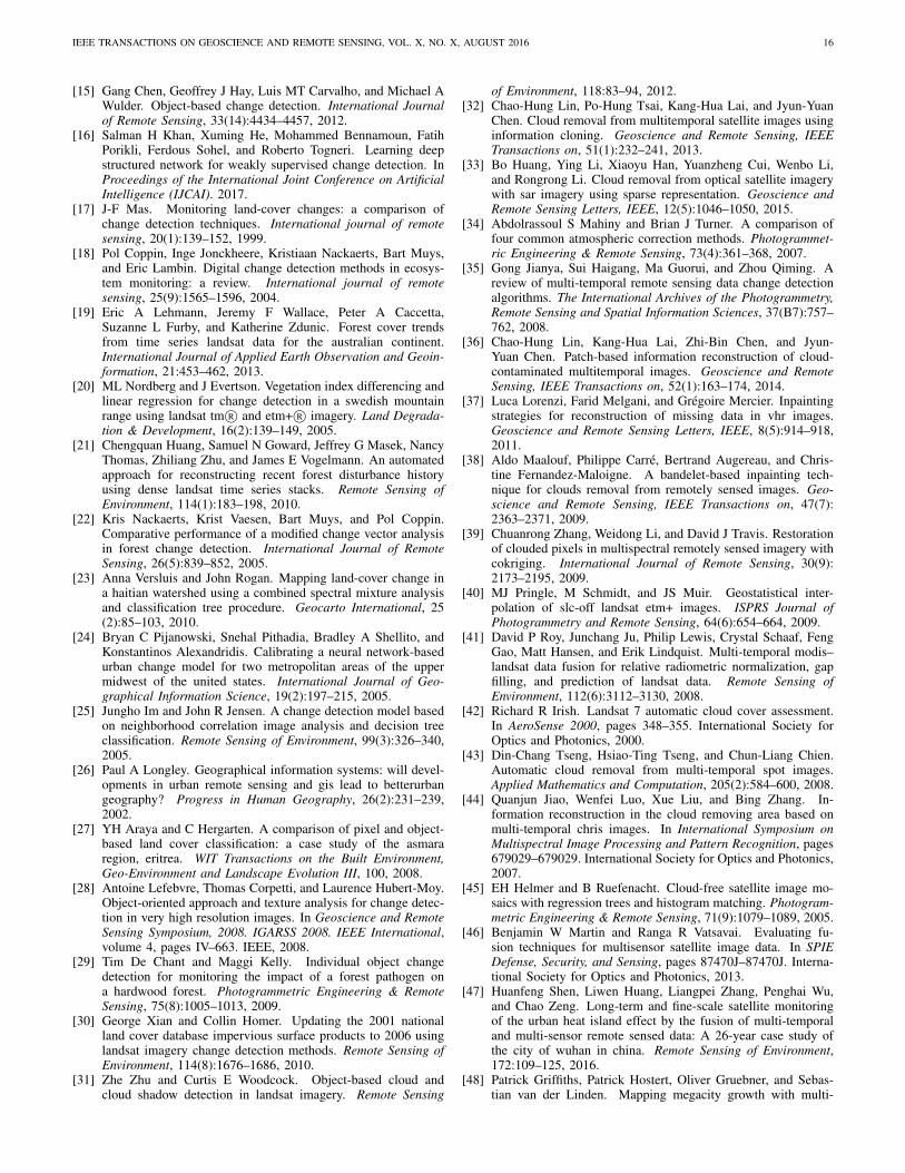
TABLE II: Db-37 Region: Patch-wise classification and detec-tion results for the temporal sequence are summarized below.All performance numbers are in percentages (%).
Method Accuracy Avg. Recall Mean IOU
SIFT+l-SVM 68.1 57.3 50.2SIFT+k-SVM 71.3 61.4 54.8SIFT+RF 69.7 58.8 50.6
BoW+l-SVM 72.6 63.1 54.8BoW+k-SVM 74.1 64.9 57.1BoW + RF 71.7 64.0 54.7
This paper 92.0 84.6 84.7
percentage coverage of the ground-truth change regions whenthe number of box proposals is increased in Fig. 10. Further-more, we have also evaluated the performance of the randombox generation around the change regions. Specifically, forrandom box generation, we obtain a thresholded change maskfor each yearly profile image and generate randomly sizedboxes with in the range of ground-truth change box sizes (byvarying the box diagonal). Afterwards, the desired number ofboxes are randomly selected as the candidate set for furtherprocessing. With the same number of boxes as the ones usedfor EdgeBox (∼ 1900), the coverage rate turned out to be verylow (17.6%). However, we noticed a consistent increase in thecoverage rate and for a very huge number of boxes (50,000),we obtained a good coverage rate of 86.7%.
We performed patch level change/no-change prediction by
TABLE III: Db-36 Region: Patch-wise classification and de-tection results for the temporal sequence are reported below.All performance numbers are in percentages (%).
Method Accuracy Avg. Recall Mean IOU
SIFT+l-SVM 69.0 57.0 54.2SIFT+k-SVM 71.8 59.3 57.8SIFT+RF 71.3 58.6 55.1
BoW+l-SVM 74.2 63.0 61.5BoW+k-SVM 76.5 65.6 64.9BoW + RF 73.9 61.5 60.0
This paper 91.3 70.8 85.4
treating the problem as a classification task. In Table II), wereport the overall accuracy, the average recall rate and themean IOU (averaged over all classes). We noticed a compara-tively higher performance when features were fused in a smallwindow along the temporal dimension to get an improvedfeature representation at each time instance. We tested differentsized windows and observed that a medium sized window(size = 7) performed best. The baseline approaches performfairly low (accuracy and recall difference as much as ∼24%and ∼27%, respectively) compared to our proposed approach.Among the two baseline techniques, the bag-of-words basedprocedure performs better than the low-level SIFT features.In terms of classifiers, the homogeneous approximation ofχ2-kernel outperforms consistently the linear SVM and RFalternatives.
IEEE TRANSACTIONS ON GEOSCIENCE AND REMOTE SENSING, VOL. X, NO. X, AUGUST 2016 12
TABLE IV: Our results for onset/offset detection and compar-isons with several baseline techniques are reported for Db-37region. The error units are months (Mn) and it is defined asthe mean taxicab distance.
Method Onset Error (Mn) Offset Error (Mn)
SIFT+l-SVM 8.7 ± 4.1 15.1 ± 7.5SIFT+k-SVM 8.3 ± 4.1 14.9 ± 7.2SIFT+RF 8.9 ± 4.3 15.9 ± 7.7
BoW+l-SVM 7.4 ± 3.6 13.5 ± 6.9BoW+k-SVM 7.1 ± 3.4 12.6 ± 6.8BoW + RF 7.4 ± 3.7 13.8 ± 7.1
This paper 3.2 ± 2.3 5.5 ± 5.5
TABLE V: Onset/offset detection results and comparisons withseveral baseline techniques are reported for Db-36 region.
Method Onset Error (Mn) Offset Error (Mn)
SIFT+l-SVM 9.2±3.7 17.4±7.7SIFT+k-SVM 8.4±3.8 15.5±7.0SIFT+RF 9.0±3.5 17.5±7.7
BoW+l-SVM 7.8±3.5 14.2±6.0BoW+k-SVM 6.8±3.1 12.9±5.7BoW + RF 7.5±3.3 14.4±6.1
This paper 4.1 ± 2.7 6.9 ± 4.8
2) Change Detection Results: For the temporal changedetection task, since it is highly unlikely to have forestchanges taking place abruptly at close-by time instances, wefurther smooth the output predictions made by the baselineprocedures. For this purpose we used a uni-dimensional me-dian filter with a comparatively higher window size of 5(equivalent to ∼10 months data). We note that the outputsfrom our CNN based approach with feature fusion are alreadysmooth and do not need further processing. Therefore, ourfinal classification and detection results which are reported inTables II and III use feature level fusion but do not use anyoutput prediction smoothing. Sample results of ground-truthand predicted sequences for the case of fire and harvest eventsare shown in Figure 13. Our approach provides temporally-smooth labelings and it was able to detect multiple changesof similar and different types occurring at a particular changesite.
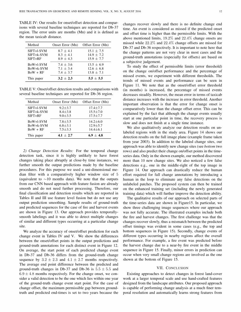
We analyze the accuracy of onset/offset prediction for eachchange event in Tables IV and V. We show the differencesbetween the onset/offset points in the output predictions andground-truth annotations for each distinct event in Figure 12.On average, the start point of each predicted change eventin Db-37 and Db-36 differs from the ground-truth changesequence by 3.2 ± 2.3 and 4.1 ± 2.7 months respectively.The average end point difference between the predicted andground-truth changes in Db-37 and Db-36 is 5.5 ± 5.5 and6.9± 4.8 months respectively. For the change onset, we con-sider a valid detection to be the one which lies within one yearof the ground-truth change event start point. For the case ofchange offset, the maximum permissible gap between ground-truth and predicted end-times is set to two years because the
changes recover slowly and there is no definite change endtime. An event is considered as missed if the predicted onsetand offset time is higher than the permissible limits. With theabove mentioned limits, 19.2% and 22.4% change onsets aremissed while 22.2% and 22.4% change offsets are missed forDb-37 and Db-36 respectively. It is important to note here thatthe change patterns are not very clear in most cases and theground-truth annotations (especially for offsets) are based ona subjective judgement.
To study the effect of permissible limits (error threshold)on the change on/offset performance and the percentage ofmissed events, we experiment with different thresholds. Thetrends of missed events and performance can be seen inFigure 11. We note that as the onset/offset error threshold(in months) is increased, the percentage of missed eventsdecreases steadily. However, the mean error in terms of taxicabdistance increases with the increase in error threshold. Anotherimportant observation is that the error for change onset iscomparatively lower than the change offset error. This can beexplained by the fact that although the change events usuallystart at one particular point in time, the recovery process isslow and does not finish at a single time instance.
We also qualitatively analyze our detection results on un-labeled regions with in the study area. Figure 14 shows ourdetection results on the full image plane (example frame takenfrom year 2003). In addition to the labeled change sites, ourapproach was able to identify new change sites (see bottom tworows) and also predict their change on/offset points in the time-series data. Only in the shown example, our method discoveredmore than 10 new change sites. We also noticed a few falsedetections e.g., one in the middle-right of the top image inFigure 14. Our approach can drastically reduce the humaneffort required for full change annotations by introducing ahuman in the loop to eliminate any false detections on theunlabeled patches. The proposed system can then be trainedon the enhanced training set (including the newly generatedtraining data) which will further improve the detection ability.
The qualitative results of our approach on selected parts ofthe time-series data are shown in Figure15. In particular, weshow three challenging image sequences where our approachwas not fully accurate. The illustrated examples include boththe fire and harvest changes. The first challenge was that thechanges recover slowly, thus a mismatch between the predictedoffset timings was evident in some cases (e.g., the top andbottom sequences in Figure 15). Secondly, change events ofdifferent types occurring in nearby regions affect the overallperformance. For example, a fire event was predicted beforethe harvest change due to a near-by fire event in the middlesequence in Figure 15. Finally, minor errors in prediction canoccur when very small change regions are involved as the oneshown at the bottom of Figure 15.
VII. CONCLUSION
Existing approaches to detect changes in forest land-coverwork at a larger temporal scale and use hand-crafted featuresdesigned from the landscape attributes. Our proposed approachis capable of performing change analysis at a much finer tem-poral resolution and automatically learns strong features from

IEEE TRANSACTIONS ON GEOSCIENCE AND REMOTE SENSING, VOL. X, NO. X, AUGUST 2016 13
0 20 40 60 80 100 120 140
Prediction time-line
Actual time-line
Frame Number
(a)
0 20 40 60 80 100 120 140
Prediction time-line
Actual time-line
Frame Number
(b)
0 20 40 60 80 100 120 140
Prediction time-line
Actual time-line
Frame Number
(c)
0 20 40 60 80 100 120 140
Prediction time-line
Actual time-line
Frame Number
(d)
0 20 40 60 80 100 120 140
Prediction time-line
Actual time-line
Frame Number
(e)
0 20 40 60 80 100 120 140
Prediction time-line
Actual time-line
Frame Number
(f)
No Change Harvest Event Fire Event
Fig. 13: (a-f) Sample results of the ground-truth change patterns and the change sequences predicted by our approach. In eachplot, the top bar shows ground truth, and the bottom bar shows prediction from our approach.
the raw surface reflectance data. To achieve a finer temporalresolution, we perform data inpainting using the reliable datavalues and sparse coding. For change detection, our approachworks on the object-level by identifying a candidate set ofchange regions using multi-resolution area profiles. We useboth spatial and temporal contextual information in the deepCNN model which helps in making better predictions. Ourmethod can precisely localize the change regions and predicttheir on/offset timings accurately within an error margin of 3to 6 months. In future, the possibility of creating a large-scaleannotated dataset will be investigated. This will enable thetraining of large-scale data driven models from scratch. Sinceinteresting changes are scarce in practical settings, we willalso investigate class-imbalanced learning of deep networksfor change detection [69].
ACKNOWLEDGEMENTS
The authors would like to thank Geoscience Australia for providingthe data and expert annotations. We gratefully acknowledge the sup-port of NVIDIA Corporation with the donation of the Tesla K40 GPUused for this research. This work is supported by Data61/CSIRO,UWA through IPRS, and under the Australian Research Council’sDiscovery Projects funding scheme (project DP150104645).
REFERENCES
[1] ABARES. Australias state of the forests five-yearly report 2013.Australian Bureau of Agricultural and Resource Economicsand Sciences (ABARES), Department of Agriculture, AustralianGovernment, 2013.
[2] Robert E Kennedy, Zhiqiang Yang, and Warren B Cohen.Detecting trends in forest disturbance and recovery using yearlylandsat time series: 1. landtrendrtemporal segmentation algo-rithms. Remote Sensing of Environment, 114(12):2897–2910,2010.
[3] Matthew C Hansen and Thomas R Loveland. A review of largearea monitoring of land cover change using landsat data. Remotesensing of Environment, 122:66–74, 2012.
[4] Masroor Hussain, Dongmei Chen, Angela Cheng, Hui Wei, andDavid Stanley. Change detection from remotely sensed images:
From pixel-based to object-based approaches. ISPRS Journalof Photogrammetry and Remote Sensing, 80:91–106, 2013.
[5] Txomin Hermosilla, Michael A Wulder, Joanne C White,Nicholas C Coops, and Geordie W Hobart. Regional detection,characterization, and attribution of annual forest change from1984 to 2012 using landsat-derived time-series metrics. RemoteSensing of Environment, 170:121–132, 2015.
[6] Ross S Lunetta, David M Johnson, John G Lyon, and JillCrotwell. Impacts of imagery temporal frequency on land-coverchange detection monitoring. Remote Sensing of Environment,89(4):444–454, 2004.
[7] Salman H Khan, Mohammed Bennamoun, Ferdous Sohel, andRoberto Togneri. Automatic shadow detection and removalfrom a single image. IEEE transactions on pattern analysisand machine intelligence, 38(3):431–446, 2016.
[8] Karen Simonyan and Andrew Zisserman. Very deep convolu-tional networks for large-scale image recognition. arXiv preprintarXiv:1409.1556, 2014.
[9] Jonathan Long, Evan Shelhamer, and Trevor Darrell. Fullyconvolutional networks for semantic segmentation. In Proceed-ings of the IEEE Conference on Computer Vision and PatternRecognition, pages 3431–3440, 2015.
[10] Salman H Khan, Munawar Hayat, Mohammed Bennamoun,Roberto Togneri, and Ferdous A Sohel. A discriminativerepresentation of convolutional features for indoor scene recog-nition. IEEE Transactions on Image Processing, 25(7):3372–3383, 2016.
[11] George Xian, Collin Homer, and Joyce Fry. Updating the 2001national land cover database land cover classification to 2006by using landsat imagery change detection methods. RemoteSensing of Environment, 113(6):1133–1147, 2009.
[12] A Kawabata, K Ichii, and Y Yamaguchi. Global monitoringof interannual changes in vegetation activities using ndvi andits relationships to temperature and precipitation. InternationalJournal of Remote Sensing, 22(7):1377–1382, 2001.
[13] Daniel Tomowski, Manfred Ehlers, and Sascha Klonus. Colourand texture based change detection for urban disaster analysis.In Urban Remote Sensing Event (JURSE), 2011 Joint, pages329–332. IEEE, 2011.
[14] Chengquan Huang, Kuan Song, Sunghee Kim, John RG Town-shend, Paul Davis, Jeffrey G Masek, and Samuel N Goward.Use of a dark object concept and support vector machinesto automate forest cover change analysis. Remote Sensing ofEnvironment, 112(3):970–985, 2008.

IEEE TRANSACTIONS ON GEOSCIENCE AND REMOTE SENSING, VOL. X, NO. X, AUGUST 2016 14
Fig. 14: This figure shows detection results on the complete image plane encompassing the forest area under investigation.We show some examples of change regions (bottom two rows) which were not labeled by the experts, yet our algorithm wassuccessfully able to detect them.

IEEE TRANSACTIONS ON GEOSCIENCE AND REMOTE SENSING, VOL. X, NO. X, AUGUST 2016 15
Idx:712 2
50 100 150 200 250 300
20
40
60
80
100
120
140
Idx:722 2
50 100 150 200 250 300
20
40
60
80
100
120
140
Idx:732 2
50 100 150 200 250 300
20
40
60
80
100
120
140
Idx:742 2
50 100 150 200 250 300
20
40
60
80
100
120
140
Idx:752 2
50 100 150 200 250 300
20
40
60
80
100
120
140
Idx:762 2
50 100 150 200 250 300
20
40
60
80
100
120
140
Idx:772 2
50 100 150 200 250 300
20
40
60
80
100
120
140
Idx:782 1
50 100 150 200 250 300
20
40
60
80
100
120
140
Idx:792 1
50 100 150 200 250 300
20
40
60
80
100
120
140
Idx:802 1
50 100 150 200 250 300
20
40
60
80
100
120
140
Idx:812 1
50 100 150 200 250 300
20
40
60
80
100
120
140
Idx:822 1
50 100 150 200 250 300
20
40
60
80
100
120
140
Idx:832 1
50 100 150 200 250 300
20
40
60
80
100
120
140
Idx:841 1
50 100 150 200 250 300
20
40
60
80
100
120
140
Idx:851 1
50 100 150 200 250 300
20
40
60
80
100
120
140
Idx:861 1
50 100 150 200 250 300
20
40
60
80
100
120
140
Idx:871 1
50 100 150 200 250 300
20
40
60
80
100
120
140
Idx:881 1
50 100 150 200 250 300
20
40
60
80
100
120
140
(a)Idx:501 1
10 20 30 40 50 60 70 80
5
10
15
20
25
30
Idx:511 1
10 20 30 40 50 60 70 80
5
10
15
20
25
30
Idx:521 1
10 20 30 40 50 60 70 80
5
10
15
20
25
30
Idx:531 1
10 20 30 40 50 60 70 80
5
10
15
20
25
30
Idx:541 2
10 20 30 40 50 60 70 80
5
10
15
20
25
30
Idx:551 2
10 20 30 40 50 60 70 80
5
10
15
20
25
30
Idx:561 2
10 20 30 40 50 60 70 80
5
10
15
20
25
30
Idx:571 2
10 20 30 40 50 60 70 80
5
10
15
20
25
30
Idx:581 2
10 20 30 40 50 60 70 80
5
10
15
20
25
30
Idx:593 2
10 20 30 40 50 60 70 80
5
10
15
20
25
30
Idx:603 2
10 20 30 40 50 60 70 80
5
10
15
20
25
30
Idx:613 3
10 20 30 40 50 60 70 80
5
10
15
20
25
30
Idx:623 3
10 20 30 40 50 60 70 80
5
10
15
20
25
30
Idx:633 3
10 20 30 40 50 60 70 80
5
10
15
20
25
30
Idx:643 3
10 20 30 40 50 60 70 80
5
10
15
20
25
30
Idx:653 3
10 20 30 40 50 60 70 80
5
10
15
20
25
30
Idx:663 3
10 20 30 40 50 60 70 80
5
10
15
20
25
30
Idx:673 3
10 20 30 40 50 60 70 80
5
10
15
20
25
30
(b)Idx:552 2
2 4 6 8 10 12 14
2
4
6
8
10
12
14
16
Idx:562 2
2 4 6 8 10 12 14
2
4
6
8
10
12
14
16
Idx:572 2
2 4 6 8 10 12 14
2
4
6
8
10
12
14
16
Idx:582 2
2 4 6 8 10 12 14
2
4
6
8
10
12
14
16
Idx:592 2
2 4 6 8 10 12 14
2
4
6
8
10
12
14
16
Idx:602 2
2 4 6 8 10 12 14
2
4
6
8
10
12
14
16
Idx:611 2
2 4 6 8 10 12 14
2
4
6
8
10
12
14
16
Idx:621 2
2 4 6 8 10 12 14
2
4
6
8
10
12
14
16
Idx:641 2
2 4 6 8 10 12 14
2
4
6
8
10
12
14
16
Idx:661 2
2 4 6 8 10 12 14
2
4
6
8
10
12
14
16
Idx:671 2
2 4 6 8 10 12 14
2
4
6
8
10
12
14
16
Idx:681 2
2 4 6 8 10 12 14
2
4
6
8
10
12
14
16
Idx:701 2
2 4 6 8 10 12 14
2
4
6
8
10
12
14
16
Idx:711 2
2 4 6 8 10 12 14
2
4
6
8
10
12
14
16
Idx:721 2
2 4 6 8 10 12 14
2
4
6
8
10
12
14
16
Idx:731 2
2 4 6 8 10 12 14
2
4
6
8
10
12
14
16
Idx:741 2
2 4 6 8 10 12 14
2
4
6
8
10
12
14
16
Idx:751 2
2 4 6 8 10 12 14
2
4
6
8
10
12
14
16
(c)
Fig. 15: Three small portions of patch sequences are shown in the above figure. The ground-truth and the predicted change/no-change labels are shown on the top left corner in blue color and red color respectively. The digits 1, 2 and 3 on top-leftrepresent no change, fire and harvest respectively.
IEEE TRANSACTIONS ON GEOSCIENCE AND REMOTE SENSING, VOL. X, NO. X, AUGUST 2016 16
[15] Gang Chen, Geoffrey J Hay, Luis MT Carvalho, and Michael AWulder. Object-based change detection. International Journalof Remote Sensing, 33(14):4434–4457, 2012.
[16] Salman H Khan, Xuming He, Mohammed Bennamoun, FatihPorikli, Ferdous Sohel, and Roberto Togneri. Learning deepstructured network for weakly supervised change detection. InProceedings of the International Joint Conference on ArtificialIntelligence (IJCAI). 2017.
[17] J-F Mas. Monitoring land-cover changes: a comparison ofchange detection techniques. International journal of remotesensing, 20(1):139–152, 1999.
[18] Pol Coppin, Inge Jonckheere, Kristiaan Nackaerts, Bart Muys,and Eric Lambin. Digital change detection methods in ecosys-tem monitoring: a review. International journal of remotesensing, 25(9):1565–1596, 2004.
[19] Eric A Lehmann, Jeremy F Wallace, Peter A Caccetta,Suzanne L Furby, and Katherine Zdunic. Forest cover trendsfrom time series landsat data for the australian continent.International Journal of Applied Earth Observation and Geoin-formation, 21:453–462, 2013.
[20] ML Nordberg and J Evertson. Vegetation index differencing andlinear regression for change detection in a swedish mountainrange using landsat tm R© and etm+ R© imagery. Land Degrada-tion & Development, 16(2):139–149, 2005.
[21] Chengquan Huang, Samuel N Goward, Jeffrey G Masek, NancyThomas, Zhiliang Zhu, and James E Vogelmann. An automatedapproach for reconstructing recent forest disturbance historyusing dense landsat time series stacks. Remote Sensing ofEnvironment, 114(1):183–198, 2010.
[22] Kris Nackaerts, Krist Vaesen, Bart Muys, and Pol Coppin.Comparative performance of a modified change vector analysisin forest change detection. International Journal of RemoteSensing, 26(5):839–852, 2005.
[23] Anna Versluis and John Rogan. Mapping land-cover change ina haitian watershed using a combined spectral mixture analysisand classification tree procedure. Geocarto International, 25(2):85–103, 2010.
[24] Bryan C Pijanowski, Snehal Pithadia, Bradley A Shellito, andKonstantinos Alexandridis. Calibrating a neural network-basedurban change model for two metropolitan areas of the uppermidwest of the united states. International Journal of Geo-graphical Information Science, 19(2):197–215, 2005.
[25] Jungho Im and John R Jensen. A change detection model basedon neighborhood correlation image analysis and decision treeclassification. Remote Sensing of Environment, 99(3):326–340,2005.
[26] Paul A Longley. Geographical information systems: will devel-opments in urban remote sensing and gis lead to betterurbangeography? Progress in Human Geography, 26(2):231–239,2002.
[27] YH Araya and C Hergarten. A comparison of pixel and object-based land cover classification: a case study of the asmararegion, eritrea. WIT Transactions on the Built Environment,Geo-Environment and Landscape Evolution III, 100, 2008.
[28] Antoine Lefebvre, Thomas Corpetti, and Laurence Hubert-Moy.Object-oriented approach and texture analysis for change detec-tion in very high resolution images. In Geoscience and RemoteSensing Symposium, 2008. IGARSS 2008. IEEE International,volume 4, pages IV–663. IEEE, 2008.
[29] Tim De Chant and Maggi Kelly. Individual object changedetection for monitoring the impact of a forest pathogen ona hardwood forest. Photogrammetric Engineering & RemoteSensing, 75(8):1005–1013, 2009.
[30] George Xian and Collin Homer. Updating the 2001 nationalland cover database impervious surface products to 2006 usinglandsat imagery change detection methods. Remote Sensing ofEnvironment, 114(8):1676–1686, 2010.
[31] Zhe Zhu and Curtis E Woodcock. Object-based cloud andcloud shadow detection in landsat imagery. Remote Sensing
of Environment, 118:83–94, 2012.[32] Chao-Hung Lin, Po-Hung Tsai, Kang-Hua Lai, and Jyun-Yuan
Chen. Cloud removal from multitemporal satellite images usinginformation cloning. Geoscience and Remote Sensing, IEEETransactions on, 51(1):232–241, 2013.
[33] Bo Huang, Ying Li, Xiaoyu Han, Yuanzheng Cui, Wenbo Li,and Rongrong Li. Cloud removal from optical satellite imagerywith sar imagery using sparse representation. Geoscience andRemote Sensing Letters, IEEE, 12(5):1046–1050, 2015.
[34] Abdolrassoul S Mahiny and Brian J Turner. A comparison offour common atmospheric correction methods. Photogrammet-ric Engineering & Remote Sensing, 73(4):361–368, 2007.
[35] Gong Jianya, Sui Haigang, Ma Guorui, and Zhou Qiming. Areview of multi-temporal remote sensing data change detectionalgorithms. The International Archives of the Photogrammetry,Remote Sensing and Spatial Information Sciences, 37(B7):757–762, 2008.
[36] Chao-Hung Lin, Kang-Hua Lai, Zhi-Bin Chen, and Jyun-Yuan Chen. Patch-based information reconstruction of cloud-contaminated multitemporal images. Geoscience and RemoteSensing, IEEE Transactions on, 52(1):163–174, 2014.
[37] Luca Lorenzi, Farid Melgani, and Gregoire Mercier. Inpaintingstrategies for reconstruction of missing data in vhr images.Geoscience and Remote Sensing Letters, IEEE, 8(5):914–918,2011.
[38] Aldo Maalouf, Philippe Carre, Bertrand Augereau, and Chris-tine Fernandez-Maloigne. A bandelet-based inpainting tech-nique for clouds removal from remotely sensed images. Geo-science and Remote Sensing, IEEE Transactions on, 47(7):2363–2371, 2009.
[39] Chuanrong Zhang, Weidong Li, and David J Travis. Restorationof clouded pixels in multispectral remotely sensed imagery withcokriging. International Journal of Remote Sensing, 30(9):2173–2195, 2009.
[40] MJ Pringle, M Schmidt, and JS Muir. Geostatistical inter-polation of slc-off landsat etm+ images. ISPRS Journal ofPhotogrammetry and Remote Sensing, 64(6):654–664, 2009.
[41] David P Roy, Junchang Ju, Philip Lewis, Crystal Schaaf, FengGao, Matt Hansen, and Erik Lindquist. Multi-temporal modis–landsat data fusion for relative radiometric normalization, gapfilling, and prediction of landsat data. Remote Sensing ofEnvironment, 112(6):3112–3130, 2008.
[42] Richard R Irish. Landsat 7 automatic cloud cover assessment.In AeroSense 2000, pages 348–355. International Society forOptics and Photonics, 2000.
[43] Din-Chang Tseng, Hsiao-Ting Tseng, and Chun-Liang Chien.Automatic cloud removal from multi-temporal spot images.Applied Mathematics and Computation, 205(2):584–600, 2008.
[44] Quanjun Jiao, Wenfei Luo, Xue Liu, and Bing Zhang. In-formation reconstruction in the cloud removing area based onmulti-temporal chris images. In International Symposium onMultispectral Image Processing and Pattern Recognition, pages679029–679029. International Society for Optics and Photonics,2007.
[45] EH Helmer and B Ruefenacht. Cloud-free satellite image mo-saics with regression trees and histogram matching. Photogram-metric Engineering & Remote Sensing, 71(9):1079–1089, 2005.
[46] Benjamin W Martin and Ranga R Vatsavai. Evaluating fu-sion techniques for multisensor satellite image data. In SPIEDefense, Security, and Sensing, pages 87470J–87470J. Interna-tional Society for Optics and Photonics, 2013.
[47] Huanfeng Shen, Liwen Huang, Liangpei Zhang, Penghai Wu,and Chao Zeng. Long-term and fine-scale satellite monitoringof the urban heat island effect by the fusion of multi-temporaland multi-sensor remote sensed data: A 26-year case study ofthe city of wuhan in china. Remote Sensing of Environment,172:109–125, 2016.
[48] Patrick Griffiths, Patrick Hostert, Oliver Gruebner, and Sebas-tian van der Linden. Mapping megacity growth with multi-
IEEE TRANSACTIONS ON GEOSCIENCE AND REMOTE SENSING, VOL. X, NO. X, AUGUST 2016 17
sensor data. Remote Sensing of Environment, 114(2):426–439,2010.
[49] Ronan Fablet and Francois Rousseau. Non-local super-resolution of missing data in multi-sensor observations of seasurface geophysical fields. In IGARSS 2015: IEEE InternationalGeoscience and Remote Sensing Symposium, pages TUP–PJ,2015.
[50] Kevin C Guay, Pieter SA Beck, Logan T Berner, Scott J Goetz,Alessandro Baccini, and Wolfgang Buermann. Vegetationproductivity patterns at high northern latitudes: a multi-sensorsatellite data assessment. Global change biology, 20(10):3147–3158, 2014.
[51] Otavio AB Penatti, Keiller Nogueira, and Jefersson A dosSantos. Do deep features generalize from everyday objects toremote sensing and aerial scenes domains? In Proceedings ofthe IEEE Conference on Computer Vision and Pattern Recog-nition Workshops, pages 44–51, 2015.
[52] Lionel Gueguen and Raffay Hamid. Large-scale damage de-tection using satellite imagery. In Proceedings of the IEEEConference on Computer Vision and Pattern Recognition, pages1321–1328, 2015.
[53] Martin Langkvist, Andrey Kiselev, Marjan Alirezaie, and AmyLoutfi. Classification and segmentation of satellite orthoimageryusing convolutional neural networks. Remote Sensing, 8(4):329,2016.
[54] Fan Hu, Gui-Song Xia, Jingwen Hu, and Liangpei Zhang.Transferring deep convolutional neural networks for the sceneclassification of high-resolution remote sensing imagery. Re-mote Sensing, 7(11):14680–14707, 2015.
[55] Munawar Hayat, Salman H Khan, Mohammed Bennamoun, andSenjian An. A spatial layout and scale invariant feature repre-sentation for indoor scene classification. IEEE Transactions onImage Processing, 25(10):4829–4841, 2016.
[56] Jun Wang, Jingwei Song, Mingquan Chen, and Zhi Yang. Roadnetwork extraction: a neural-dynamic framework based on deeplearning and a finite state machine. International Journal ofRemote Sensing, 36(12):3144–3169, 2015.
[57] Xueyun Chen, Shiming Xiang, Cheng-Lin Liu, and Chun-HongPan. Vehicle detection in satellite images by hybrid deepconvolutional neural networks. IEEE Geoscience and remotesensing letters, 11(10):1797–1801, 2014.
[58] Richard R Irish, John L Barker, Samuel N Goward, and TerryArvidson. Characterization of the landsat-7 etm+ automatedcloud-cover assessment (acca) algorithm. PhotogrammetricEngineering & Remote Sensing, 72(10):1179–1188, 2006.
[59] Fuqin Li, David LB Jupp, Shanti Reddy, Leo Lymburner,Norman Mueller, Peter Tan, and Anisul Islam. An evaluationof the use of atmospheric and brdf correction to standardizelandsat data. Selected Topics in Applied Earth Observationsand Remote Sensing, IEEE Journal of, 3(3):257–270, 2010.
[60] Fuqin Li, David LB Jupp, Medhavy Thankappan, Leo Lym-burner, Norman Mueller, Adam Lewis, and Alex Held. Aphysics-based atmospheric and brdf correction for landsat dataover mountainous terrain. Remote Sensing of Environment, 124:756–770, 2012.
[61] Julien Mairal, Francis Bach, Jean Ponce, and Guillermo Sapiro.Online learning for matrix factorization and sparse coding. TheJournal of Machine Learning Research, 11:19–60, 2010.
[62] Stephane G Mallat and Zhifeng Zhang. Matching pursuitswith time-frequency dictionaries. Signal Processing, IEEETransactions on, 41(12):3397–3415, 1993.
[63] C Lawrence Zitnick and Piotr Dollar. Edge boxes: Locatingobject proposals from edges. In European Conference onComputer Vision 2014, pages 391–405. Springer, 2014.
[64] Piotr Dollar and C. Lawrence Zitnick. Structured forests for fastedge detection. In Proceedings of the International Conferenceon Computer Vision, 2013.
[65] A. Vedaldi and A. Zisserman. Efficient additive kernels viaexplicit feature maps. In Proceedings of the IEEE Conference
on Computer Vision and Pattern Recognition, 2010.[66] Jasper RR Uijlings, Koen EA van de Sande, Theo Gevers, and
Arnold WM Smeulders. Selective search for object recognition.International journal of computer vision, 104(2):154–171, 2013.
[67] Joao Carreira and Cristian Sminchisescu. Cpmc: Automatic ob-ject segmentation using constrained parametric min-cuts. IEEETransactions on Pattern Analysis and Machine Intelligence, 34(7):1312–1328, 2012.
[68] Bogdan Alexe, Thomas Deselaers, and Vittorio Ferrari. Mea-suring the objectness of image windows. IEEE Transactions onPattern Analysis and Machine Intelligence, 34(11):2189–2202,2012.
[69] Salman H Khan, Mohammed Bennamoun, Ferdous Sohel,and Roberto Togneri. Cost sensitive learning of deep fea-ture representations from imbalanced data. arXiv preprintarXiv:1508.03422, 2015.
Salman Khan (M’15) received the B.E. degree inelectrical engineering from the National Universityof Sciences and Technology (NUST), Pakistan, in2012, and the Ph.D. degree from The University ofWestern Australia (UWA), in 2016. He was a Vis-iting Researcher with National ICT Australia, CRL,during the year 2015. He is currently a Research Sci-entist with Data61 (CSIRO) and an Adjunct Lecturerwith Australian National University (ANU) since2016. His research interests include computer vision,pattern recognition and machine learning.
Xuming He received the Ph.D. degree in computerscience from the University of Toronto, Canada, in2008. He was an Adjunct Research Fellow with Aus-tralian National University from 2010 to 2016. Heheld a post-doctoral position with the University ofCalifornia at Los Angeles, USA, from 2008 to 2010.He joined National ICT Australia and was a SeniorResearcher from 2013 to 2016. He is currently anAssociate Professor with the School of InformationScience and Technology, ShanghaiTech University.His research interests include semantic image and
video segmentation, 3-D scene understanding, visual motion analysis, andefficient inference and learning in structured models.
Fatih Porikli (M’99-F’13) received the Ph.D. degreefrom New York University in 2002. He was theDistinguished Research Scientist with MitsubishiElectric Research Laboratories. He is currently aProfessor with the Research School of Engineering,Australian National University and a Chief Scientistat the Global Media Technologies Lab at Huawei,Santa Clara. He has authored over 150 publications,coedited two books, and invented 66 patents. Hisresearch interests include computer vision, patternrecognition, manifold learning, image enhancement,
robust and sparse optimization and online learning with commercial appli-cations in video surveillance, car navigation, robotics, satellite, and medicalsystems. He was a recipient of the Research and Development 100 Scientist ofthe Year Award in 2006. He received five Best Paper Awards at premier IEEEconferences and five other professional prizes. He is serving as the AssociateEditor of several journals for the past 12 years.
Mohammed Bennamoun received his M.Sc. degreein control theory from Queen’s University, Kingston,Canada, and the Ph.D. degree in computer visionfrom Queen’s University/Queensland University ofTechnology (QUT), Brisbane, Australia. He lecturedRobotics at Queen’s University and then joined QUTin 1993 as an Associate Lecturer. He is currently aWinthrop Professor and has been the Head of theSchool of Computer Science and Software Engineer-ing, The University of Western Australia (UWA),Perth, Australia for five years (2007−2012). He has
published over 300 journal and conference publications and secured highlycompetitive national grants from the Australian Research Council (ARC). Hisareas of interest include control theory, robotics, object recognition, artificialneural networks, signal/image processing, and computer vision.