ieee transactions on geoscience and remote …...ieee transactions on geoscience and remote sensing,...
TRANSCRIPT
IEEE TRANSACTIONS ON GEOSCIENCE AND REMOTE SENSING, VOL. GE-24, NO, I, JANUARY 1986
Detection and Evaluation of Plant Stresses for CropManagement Decisions
RAY D. JACKSON, PAUL J, PINTER, JR., ROBERT J. REGlNATO, AND SHERWOOD B. IDSO
99
Abstract-The ability to quantitatively assess crop conditions usin~remotely sensed data would not only improve yield forecasts but wouldalso provide information that would be useful to farm managers inmakin~ day-to-day mana~ement decisions. Experiments were con-ducted using ~round-based radiometers to relate spectral response tocrop canopy characteristics. It was found that radiometrically mea-sured crop temperature, when compared with a reference tempera-ture, was related to the de~ree of plant stress and could indicate theonset of stress. Reflectance based ve~etation indices, on the other hand,were not sensitive to the onset of stress but were useful in evaluatingthe consequences of stress as expressed in chan~in~ quantities of greenphytomass. Anatomical and physiological chan~es occur within plantcells when plants are stressed and increase the amount of reflected ra-diation. However, canopy geometrical chan~es may alter the amount ofradiation that reaches a radiometer, complicatin~ the interpretation ofspectral response to stress. Timeliness, frequency of covera~e, and res-olution are three factors that must be considered when satellite-basedsensors are used to evaluate crop conditions for farm mana~ement ap-plications.
1. INTRODUCTION
THE POTENTIAL yield of any crop can be realizedonly when water, nutrient, and environmental condi-
tions are optimum, and if disease and insect problems areminimized or prevented. Whenever plant growth is re-tarded by less than optimum conditions, the plants are saidto be stressed. The word "stress", although difficult todefine from a physiological point of view, is commonlyused to signify any effect on plant growth that is detri-mental. The term "crop condition" implies an evaluationof the degree of stress. Visual assessment of crop stressis qualitative at best, with the terms "good" or "poor"frequently used to describe crop condition.
The quantification of plant stress using remotely senseddata was a major objective of several research projectsconducted under the AgRISTARS program. Although theresearch goal was to quantify crop stress using satellitedata, it was necessary to conduct a number of experimentsusing ground-based radiometers. These instruments wereused over controlled plots with known stress conditionsand with known plant and soil parameters to obtain thedata base required to relate the remotely sensed measure-ment to a degree of crop stress.
During the course of the experiments it became appar-
ManuscriptreceivedMay25, 1985; revisedAugust 10. 1985,The authorsare with the U,S, Departmentof Agriculture.Agricultural
Research Service. U,S, Water Conservation Laboratory, Phoenix. AZ85040,
IEEE LogNumber8406220,
ent that a number of factors can complicate the assessmentof stress when interpreting remotely sensed data. Ob-viously, some frame of reference is required if a numericalvalue is to be assigned to a stress condition. Furthermore,the spectral response of plant canopies is related to geo-metrical as well as physiological factors. In some cases,differences in spectral response of two plant canopies maybe due to leaf orientation, not to different stress condi-tions. When plants are stressed leaves may droop and curl,causing geometrical as well as physiological changes thataffect the radiation received by a remote sensor.
The results obtained using ground-based instrumentsshould prove useful for improving stress assessment tech-niques using satellite data. A quantitative measure of stressfrom space platforms would not only improve our abilityto forecast yields, but would also provide informationwhich would aid farm managers in making day-to-daymanagement decisions.
This report discusses some research results concerningthe detection and quantification of plant stresses by re-mote means, examines some complicating factors in theinterpretation of data, and assesses progress made inadapting remote sensing technology to provide day-by-dayinformation on soil and crop conditions for use by farmoperators in making farm management decisions.
II. DETECTION AND QUANTIFICATIONOF PLANT STRESS
Thermal-IR techniques can be used to detect and, insome cases, quantify plant stress. Although plant temper-atures can indicate the occurrence of stress, they cannotidentify its cause. If transpiration is restricted because ofa deficit of water (water stress) [I], or by the reduction ofthe number of conducting vessels by disease or insects (bi-ological stress) [2], or by high salinity in the soil water(salinity stress) [3], the net result is an increase in planttemperature.
When plants are stressed, physiological changes thattake place within leaves may alter their light absorptionand transmittance properties. This, along with plant ge-ometry changes such as wilting and leaf curl, can affectthe amount of reflected and emitted radiation that reachesa remote sensor. Often, by the time stress can be ascer-tained by measurements of reflected solar radiation, visualsigns are evident, and yield reducing damage has alreadyoccurred. Thus, plant temperatures indicate the onset anddegree of stress at a particular time, whereas reflected so-lar measurements integrate the effects of stress over time.
U.S. Government work not protected by U.S. copyright
lOll IEEE TRANSArTIONS ON GEOSCIENCE AND RE\lOTE SEt\SING. VOL. GE-24. NO. I. JANLARY 19R6
A. Water Stress
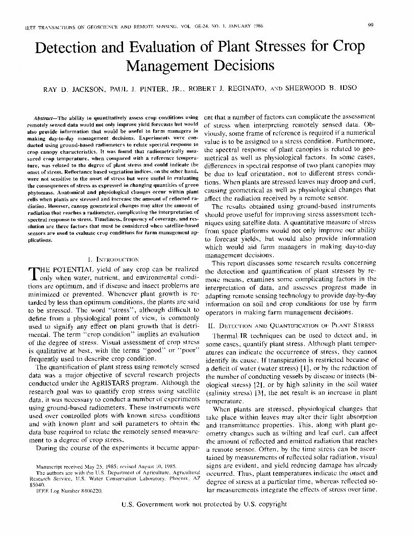
VAPOR PRESSURE DEFICIT CKPA)Fig. l. Theoretical relationship between the canopy-air temperature dif-
ference and air vapor pressure deficit. Numbers at the end of the linesindicate the value oj"the canopy resistance (r,) used t<)r the calculations.
that the canopy-air temperature difference is linearly re-lated to the air vapor pressure deficit (VPD). This rela-tion, derived from energy balance considerations, can beexpressed as 14], [II]
(I)
(2)
so
500
'Y (I + r/r(/)
Ll + 'Y(I + r/r(/)
VPD
~ + 'Y(I + r/rJ
LJVZLJa::LJLLLL~0
[l.
L -5LJf--
::':<r:
-10I>-[l.az<r:v -, 5
-200
where r" and r, are the aerodynamic and canopy resis-tances (s . m-I
), R" is the net radiation (W . m-2), pCp
the volumetric heat capacity of air (J . m-3 • C-1), 'Y isthe psychrometric constant (Pa . C-I), and ~ is the slopeof the temperature-saturated vapor pressure relation (Pa .C-I).
For well-watered plants the canopy resistance (r,) is lowbut usually not zero [13]. Assuming that 5 s . m - I is rep-resentative of r, at potential evapotranspiration, T, - T(/was calculated as a function of VPD. Results of these cal-culations are given in Fig. I. Also ~:hown are lines for r,= 50,500, and 00, which correspond to moderate, severe,and infinite stress, respectively. When r, = 00, (I) reducesto
which shows that the upper limit of plant temperature isdependent on the aerodynaP.1ic resistance and the net ra-diation.
The point B in Fig. I represents a measured value of Tc- TO' The points A and C represent the values of T, - T(/that would occur if the plants were under maximum andminimum stress, at a particular value of VPD. A cropwater stress index (CWSI) was defined as the ratio of thedistances BC/AC [!OJ, [II]. The mathematical equivalent
The potential of using infrared thermometers to mea-sure canopy temperatures was demonstrated over two de-cades ago II], [41. Since then, four indices, based on in-frared temperature measurements, have been proposed forthe quantification of plant water stress. They arc: stress-degree-day (SOD) [51, [6], which is the canopy-air tem-perature difference measured post-noon near the time ofmaximum heating; the canopy temperature variability(CTV) [71, [8], which is the variability of temperaturesencountered in a field during a particular measurement pe-riod; the temperature-stress-day (TSD) [9], which is thedifference in canopy temperature between a stressed cropand a nonstressed reference crop; and the crop water stressindex (CWSI) 110], [II j, which includes the vapor pres-sure deficit of the air in relating the canopy and air tem-perature difference to water stress. Although these indiceswere developed to quantify water stress, they are usefulfor evaluating any type of stress that causes a rise of planttemperature.
In the development of the stress-degree-day, it was as-sumed that effects of environmental factors (such as vaporpressure, net radiation, and wind) would be largely man-ifested in the canopy temperature, and that the differencebetween the canopy temperature (7;) and the air temper-ature (TJ would be a relatively useful indicator of plantwater stress. It was later demonstrated that the SOD wasinsufficient to assess water stress in corn [7]. Gardner etal. 17] showed that stressed corn plants were below airtemperature much of the time, and suggested that cornmay be more sensitive to water stress than wheat. Theyalso suggested that canopy-air temperature differencesmay be soil, crop, and climate specific.
The basis for the canopy temperature variability (CTV)index is that soils are inherently nonhomogeneous, caus-ing some areas within a field to become stressed beforeothers. Consequently, canopy temperatures would show agreater variability as water becomes limiting than theywould under well watered conditions. This variability canbe used to signal the onset of water deficits [7], [12].Gardner et al. [7] found standard deviations of 0.3°C infully irrigated plots of corn. In nonirrigated plots, thestandard deviation was as great as 4.2 DC. They concludedthat plots which exhibited a standard deviation above 0.3°Cwere in need of irrigation.
The difference in temperature between a stressed plotand a well watered plot (called the temperature stress day(TSD) by Gardner et al. 181) can also be used as a waterstress indicator. Clawson and Blad [9J tested this conceptas to its usefulness for scheduling irrigations. Their cornplots were irrigated when the average of all canopy tem-peratures measured in the stressed plot during a particulartime period were I DC warmer than the average canopytemperatures of the well watered plot. These experimentsindicated that both methods, the CTV and the TSD, couldbe used to evaluate water stress.
The crop water stress index (CWSI) is based on the fact
JACKSON e/ al.: DETECTION AND EVALUATION OF PLANT STRESS
wVZw0::wLLLL
C;Q
Ci -5f-
::<r:I -10
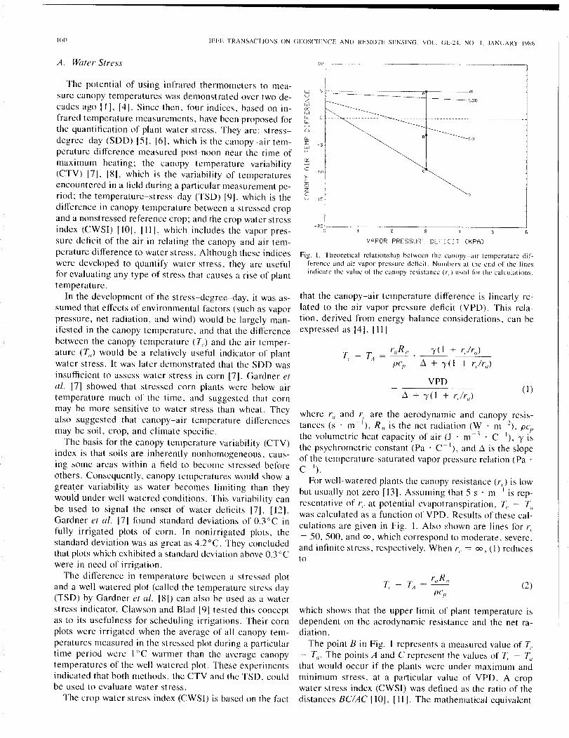
>-Qaz<r::: SLOPE =-1.96V -15 INTER = 0.58
Rt2 = O. 92
-20 oVAPOR PRESSURE DEFICIT CKPA)
101
30
0
~ 25<I:oc0 20Woc"-0W ISoc<I:ocL.... toZ
oc<I: 5WZ
030 60 90 120 150
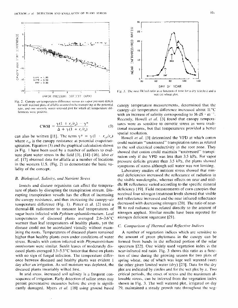
DAY or YEARFig. 3. The near-IR/red ratio as a function of time j()r a dry (circles) and a
wet (x) wheat plot.
Fig. 2. Canopy-air temperature difference versus air vapor pressure deficitfor well-watered plots of alfalfa assumed to be transpiring at the potentialrate, and one severely water-stressed plot for which all temperature dif-ferences were positive.
)'(1 + r/ra) - )'*
Ll + )' (1 + r/ra)
can also be written [11]. The term )'* = )' (1 + r,/r(/)where r(i' is the canopy resistance at potential evapotran-spiration. Equation (3) and the graphical calculation shownin Fig. 1 have been used by a number of authors to eval-uate plant water stress in the field [3], [14]-[16]. Idso etal. [17] obtained data for alfalfa at a number of locationsin the western U.S. (Fig. 2) to demonstrate the basic va-lidity of the concept.
B. Biological, Salinity, and Nutrient Stress
Insects and disease organisms can affect the tempera-ture of plants by disrupting the transpiration stream. Dis-rupting transpiration vessels has the effect of increasingthe canopy resistance, and thus increasing the canopy-airtemperature difference (Fig. 1). Pinter et al. [2] used athermal-IR radiometer to measure leaf temperatures ofsugar beets infected with Pythium aphanidermatum. Leaftemperatures of diseased plants averaged 2.6-3.6°Cwarmer than leaf temperatures of healthy plants, yet thedisease could not be ascertained visually without exam-ining the roots. Temperatures of diseased plants remainedhigher than healthy plants even under conditions of waterstress. Results with cotton infected with Phymatotrichumomnivorum were similar. Sunlit leaves of moderately dis-eased plants averaged 3.3-5.3°C hotter that those on plantswith no sign of fungal infection. The temperature differ-ence between diseased and healthy plants was evident Iday after an irrigation. As soil moisture was depleted, thediseased plants invariably wilted first.
In arid areas, increased soil salinity is a frequent con-sequence of irrigation. Early detection of saline areas maypermit preventative measures before the crop is signifi-cantly damaged. Myers et al. [18] using ground based
CWSI (3)
canopy temperature measurements, determined that thecanopy-air temperature difference increased about 11°Cwith an increase of salinity corresponding to 16 dS . m -1.
Recently, Howell et al. [3] found that canopy tempera-tures were as sensitive to osmotic stress as were tradi-tional measures, but that temperatures provided a betterspatial resolution.
Howell et at. [31 determined the VPD at which cottoncould maintain "unstressed" transpiration rates as relatedto the soil electrical conductivity in the root zone. Theyshowed that cotton could maintain "unstressed" transpi-ration only if the VPD was less than 3.5 kPa. For vaporpressure deficits greater than 3.5 kPa, the plants showedsymptoms of stress although soil water was not limiting.
Laboratory studies of nutrient stress showed that min-erai deficiencies increased the reflectance of radiation inthe visible wavelengths, whereas effects on near and mid-dle IR reflectance varied according to the specific mineraldeficiency [19]. Field measurements of corn canopies thatreceived four nitrogen treatment levels showed that visiblered reflectance increased and the near infrared reflectancedecreased with decreasing nitrogen [20]. The ratio of near-IR to red radiance was related directly to the amount ofnitrogen applied. Similar results have been reported fornitrogen deficient sugarcane [21].
C. Comparison of Thermal and Reflective Indices
A number of vegetation indices which are sensitive tothe amount of green phytomass in the canopy can beformed from bands in the reflected portion of the solarspectrum 1221. One widely used vegetation index is thenear-infrared red ratio. Fig. 3 shows this ratio as a func-tion of time during the growing season for two plots ofspring wheat, one of which was kept well watered (wet)the other given limited water (dry) [23]. Data for the dryplot are indicated by circles and for the wet plot by x. Twocritical periods, the onset of stress and the maximum al-lowable stress, can be inferred from the vegetation indexshown in Fig. 3. The well watered plot, irrigated on day79, maintained a steady growth rate throughout the veg-
102IEEE TRANSACTIONS ON GEOSCIENCE AND RE\IOTE SENSING, VOL GE-24. NO. 1. JANUARY 1986
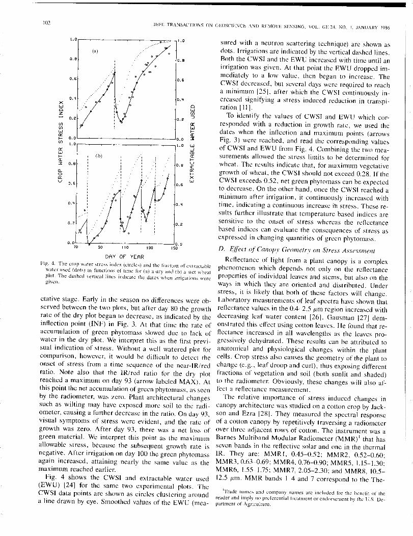
DAY or YEARFig. 4. The crop water "tress index (circles) and the fraction of extractable
water used (dots) as functions of time lur (a) a drv and (b) a wet wheatplot. The dashed vertical lines indicate the dates ~vhen irrigations weregiven.
etative stage. Early in the season no differences were ob-served between the two plots, but after day 80 the growthrate of the dry plot began to decrease, as indicated by theinflection point (INF) in Fig. 3. At that time the rate ofaccumulation of green phytomass slowed due to lack ofwater in the dry plot. We interpret this as the first previ-sual indication of stress. Without a well watered plot forcomparison, however, it would be di ftlcult to detect theonset of stress from a time sequence of the near-IR/redratio. Note also that the IR/red ratio for the dry plotreached a maximum on day 93 (arrow labeled MAX). Atthis point the net accumulation of green phytomass, as seenby the radiometer, was zero. Plant architectural changessuch as wilting may have exposed more soil to the radi-ometer, causing a further decrease in the ratio. On day 93,visual symptoms of stress were evident, and the rate ofgrowth was zero. After day 93, there was a net loss ofgreen material. We interpret this point as the maximumallowable stress, because the subsequent growth rate isnegative. After irrigation on day 100 the green phytomassagain increased, attaining nearly the same value as themaximum reached earlier.
Fig. 4 shows the CWSI and extractable water used(EWU) [24] for the same two experimental plots. TheCWSI data points are shown as circles clustering arounda line drawn by eye. Smoothed values of the EWU (mea-
'Trade names and company names are included f,)r the benefit of thereader and imply no preferential treatment or endorsement by the U.S. De-partment of Agriculture.
sured with a neutron scattering technique) are shown asdots. Irrigations are indicated by the vertical dashed lines.Both the CWSI and the EWU increased with time until anirrigation was given. At that point the EWU dropped im-mediately to a low value, then began to increase. TheCWSI decreased, but several days were required to reacha minimum [25], after which the CWSI continuously in-creased signifying a stress induced reduction in transpi-ration [II].
To identify the values of CWSI and EWU which cor-responded with a reduction in growth rate, we used thedates when the inflection and maximum points (arrowsFig. 3) were reached, and read the corresponding valuesof CWSI and EWU from Fig. 4. Combining the two mea-surements allowed the stress limits to be determined forwheat. The results indicate that, for maximum vegetativegrowth of wheat, the CWSI should not exceed 0.28. If theCWSI exceeds 0.52, net green phytomass can be expectedto decrease. On the other hand, once the CWSI reached aminimum after irrigation, it continuously increased withtime, indicating a continuous increase ih stress. These re-sults further illustrate that temperature based indices aresensitive to the onset of stress whereas the reflectancebased indices can evaluate the consequences of stress asexpressed in changing quantities of green phytomass.
D. Effect of Canopy Geometry on Stress Assessment
Reflectance of light from a plant canopy is a complexphenomenon which depends not only on the reflectanceproperties of individual leaves and stems, but also on theways in which they are oriented and distributed. Understress, it is likely that both of these factors will change.Laboratory measurements of leaf spectra have shown thatreflectance values in the 0.4--2.5 {tm region increased withdecreasing leaf water content [26]. Gausman [271 dem-onstrated this effect using cotton leaves. He found that re-flectance increased in all wavelengths as the leaves pro-gressively dehydrated. These results can be attributed toanatomical and physiological changes within the plantcells. Crop stress also causes the geometry of the plant tochange (e.g., leaf droop and curl), thus exposing differentfractions of vegetation and soil (both sunlit and shaded)to the radiometer. Obviously, these changes will also af-fect a reflectance measurement.
The relative importance of stress induced changes incanopy architecture was studied on a cotton crop by Jack-son and Ezra [28]. They measured the spectral responseof a cotton canopy by repetitively traversing a radiometerover three adjacent rows of cotton. The instrument was aBarnes Multiband Modular Radiometer (MMR)! that hasseven bands in the reflective solar and one in the thermalIR. They are: MMRI, 0.45-0.52; MMR2, 0.52-0.60;MMR3, 0.63-0.69; MMR4, 0.76-0.90; MMR5, 1.15-1.30;MMR6, 1.55-1.75; MMR7, 2.05-2.30; and MMR8, 10.5-12.5 ILm. MMR bands 1-4 and 7 correspond to the The-
1.0
0.8
0.6
O.~QW(f)
0.2::)0::Wt-<I:
0.0 3
1.0 W.-JCD<I:t-
0.8 V<I:0::t-XW
0.6
O.~
0.2
0.015013011090
xWQZ•.....(f)(f)W0::t- 0.0(f)
1.00::w
(b)t- I , ,<I: , I ,3: 0.8
,I ,, I ,
0-I .' ,I ., ,
0 , , ,0:: I I IV I I
0.6 , ,, II,,,
o.~ ,,,0' ,,

JACKSON el al.: DETECTION AND EVALUATION OF PLANT STRESS 103
Fig. 6. Reflectance factor as a function of wavelength as measured overwater lily, guayule, and water.
WAUELENGTH2.42.01.51.20.8
(L 0.5r'2 0.4L;a:LL
1100
& MMR 1
[3 MMR 2e MHR 3
x MMR '"., MMR S
_MMR 6
• MMR 7
+ MMR 8
103010000930
20
-300900
-20
W 10
'"Z<I:IuI- 0--Zwu0:::r -10
TIME or DAYFig. 5. Observed changes in cotton canopy reflectance and temperature as
a function of time after plants were stressed by severing the main stemnear the soil. Data are expressed as a percentage of energy reflected oremitted at the same time from two adjacent rows of cotton that were notstressed
matic Mapper bands 1-4 and 7, MMR6 to TM5, andMMR8 to TM6.
After an initial sequence of measurements, the stems ofthe center row of cotton were cut at a point just above thesoil. Care was taken to minimize disturbance of the can-opy structure. The cut plants were supported by woodendowels that had been inserted in the soil and to which thestems had been tied the previous day. The subsequent des-iccation of plants within this row was followed by com-paring its reflectance and emittance with a control row.
Visual signs of wilting were apparent almost immedi-ately after cutting. The uppermost leaves began to curland droop first, exposing normal appearing leaves below.Then wilting progressed slowly to the lower leaves. At theend of the experiment even the lowermost leaves showedsigns of wilt. As a consequence of wilting, the geometryof the canopy rapidly changed. Prior to cutting the leaveswere predominately horizontal. As wilting progressed theleaves became more vertical. The laboratory analysis ofGausman [27] had indicated that reflectance increased inall wavelengths with increasing water stress due to phys-iological changes of the leaves. Field results indicate thatthe reflectance may increase at some wavelengths and de-crease at others, depending on the geometry changes thataccompany stress. The data in Fig. 5 show that, for thisvariety of cotton, geometry changes playa major role indetermining reflectance properties of canopies. The re-flectance of six of the seven reflected solar bands de-creased as the cotton leaves dehydrated and the leaf angleschanged from horizontal to vertical. Our explanation issimilar to that of Holben et al. [29] in that, due to leafdroop, first surface reflections were scattered into the can-opy with less radiance reaching the sensor held above thecanopy. For the six bands, geometric effects overshad-owed the increased reflectance that occurred due to phys-iological changes.
Reflectance in the red (0.63-0.69 Jim) showed a net in-crease. The same geometrical factors were active, but thephysiological changes were apparently greater. Radiationin this band (known as the chlorophyll absorption band) isabsorbed by green leaves and provides the energy to com-bine carbon dioxide and water in the complex biochemicalprocess of photosynthesis. In a recent review, Krieg [30]concluded that the first effect of a reduction in water avail-ability would be a reduction in this biochemical processwhich would subsequently trigger the closure of stomatato reduce the exchange of carbon dioxide and water withthe atmosphere. Our hypothesis is that the sudden inter-ruption of transpiration immediately affected the photo-synthesis process causing some of the red radiation thatwas previously absorbed to be reflected back to the envi-ronment.
On a percentage basis, the visible bands reacted as rap-idly to a suddenly induced stress as did the temperature(Fig. 5). A water absorption band (2.05-2.35 Jim) de-creased by 17 percent within 10 min of a suddenly inducedstress, whereas the red band (0.63-0.67 Jim) increased byabout 12 percent within the same time period. The near-IR (0.76-0.90 Jim) showed the least percent change. Thisresult is contrary to the results of Holben et al. [29] whofound that the near-IR was the most sensitive to stress. Ingeneral, our results support the statement of Knipling [26]that the visible reflectance region is as sensitive to stressas is the near infrared region. However, in the visible re-gion the reflectance values are sufficiently small that stresscaused changes may not be detectable in an operationalmode.
Although the reflectance factor for water in all TMbands is low (Fig. 6), the mid-IR bands (1.55-1.75 Jim and2.05-2.35 Jim) are proportedly sensitive to liquid water inplant tissues. On this basis, one could assume that thesebands would be useful in detecting water stress in plants.Yet, even when liquid water is present in a scene, the ge-ometry of the scene components can be the dominant fac-tor and can cause confusion in interpreting the data. Forexample, the bidirectional reflectance factor was mea-sured over a water surface containing water lilies (Nupharluteum Sibth. & Sm.) and over a stand of the drought

104 IEEE TRANSACTIONS ON GEOSClENCE AND REMOTE SENSING, VOL. GE-24, NO. I. JANUARY 1986
Fig. 7. Relative usefulness of remotely sensed data to fanners in relationto time from acquistion to delivery in usable form.
adapted desert shrub, guayule (Parthenium argentatumGray). The water lily leaves covered about 80 percent ofthe surface area, leaving about 20 percent water exposed.The guayule shrubs were about 0.5 m tall, approaching80-90 percent cover, and in need of water. At first glanceone would think that the reflectance factor for the mid-IRbands over the water lily would be small due to absorptionby the water surface and the liquid water in the large greenleaves. However, the reflectance factor (measured at nadir)for water lily was greater than for guayule in all bandsexcept the red (Fig. 6). The flat water lily leaves causedradiation to be reflected upward toward the radiometer,whereas the guayule canopy caused more radiation to bescattered horizontally than vertically. This extreme casedemonstrates the fact that canopy geometry must be ac-counted for when interpreting reflectance factor data.
UlUJWZ~:=Jl~W1.0
w>
sT IME CDAYS)
10
ACQUISITION FREQUENCY (DAYS)Fig. 8. Relative usefulness of remole1y sensed data to farmers in relalion
to frequency of coverage.
optimum data delivery time of minutes, and a maximumtime of a few hours.
20
1.01.0WZ~:=Ju...W1.0:=JW>r-<I:~LJa:
0 10
B. Frequency of Coverage
Frequency of coverage is another important aspect. Fig.8 shows a hypothetical relationship between usefulness andfrequency. For farm management, the maximum useful-ness would obtain if continuous coverage were available.During the growing season crop conditions continouslychange. In arid areas, irrigation may be required every 7to 20 days. A system with a 16-day repeat time wouldprovide little useful information. Also, cloud conditionsmay increase the time period between acquistions. Con-tinuous coverage would be the optimum, with once a daycoverage as a mInImum.
C. Resolution
The resolution requirements for a farm managementsystem are dependent upon the particular application forthe data. For a farm with relatively uniform soils and aminimum field size of about 40 acres, the 30 x 30 m res-olution of a sensor such as the Thematic Mapper may be
III. REMOTE SENSING AS A FARM MANAGEMENT TOOL
Thermal infrared radiometry is extensively used by re-searchers for plant water stress assessment and is begin-ning to be used by farm operators. At present, portions offields are surveyed with hand-held instruments that dis-play surface temperature. The degree of stress is inferredby comparison with other fields or by combining the tem-peratures with ancillary data such as air temperature andvapor pressure. Surface temperatures derived from satel-lite data have been used for qualitative stress assessmentin a research mode, but operational systems have not yetbeen developed. Using ground based instruments to coveran entire farm is prohibitive from the point of view of timeand manpower requirements.
Reflected solar radiation has been extensively measuredusing hand-held and boom-mounted instruments for re-search purposes. Satellite data are being used for yieldforecasting and qualitative crop condition assessment.Vegetation maps derived from NOAA's AVHRR data havebeen produced for the continent of Africa [31], and areroutinely produced for the U.S. [32]. This type of infor-mation is very useful for detecting large scale vegetationchanges but is not sufficient for providing crop conditionassessment at the farm field level. In order to accomplishthe latter, problems of timeliness, frequency of coverage,and spatial resolution of a space-based system must be ad-dressed.
A. TimelinessTimeliness is perhaps the most important requirement
for a farm management remote sensing system. Fig. 7 isa hypothetical relation that shows how the usefulness ofremotely sensed data decays with time. To obtain maxi-mum usefulness, the data must be available within min-utes, This may appear extreme, but farm operations mustbe carried out when crop conditions demand. A remotesensing system that required, say, 5 days after acquisitionfor data delivery would be essentially useless for indicat-ing when to irrigate, because yield reducing damage wouldhave occurred by the time water could be applied. A re-mote-sensing system for farm management would have an

JACKSON et al.: DETECTION AND EVALUATION OF PLANT STRESS
adequate. However, this is usually not the case. Manyfields are considerably smaller than 40 acres, and soil het-erogeneity across fields causes plant growth differences.As an example, during irrigation, areas with low waterinfiltration may not have the root zone replenished withwater, whereas areas of high intake would. The irrigationprogram for that field would probably be decided on thebasis of availability and cost of water and the current crop.A farmer may decide to over irrigate the high intake areasto assure good crop development over the entire field. Un-der limited water conditions the high intake areas may beused as the indicator of when to irrigate with the loweryields on the other areas accepted. Considering a numberof factors, it appears that a resolution of 5 X 5 m wouldbe optimum, with 20 X 20 m acceptable, if sensor designconstraints will not allow a smaller figure.
IV. CONCLUDING REMARKS
Methods for detecting and quantifying crop stress usingground-based instruments are reasonably well developed.The identification of the cause of stress remains ambigu-ous. Water stress, being more ubiquitous, is usually thefirst suspect when stress is detected. However, nutrientdeficiencies may cause stress symptoms that can be con-fused with water stress. When stress is caused by morethan one factor, remotely sensed data may not provideenough information to identify the factors. For example,spectral detection of nutrient deficiencies have been dem-onstrated only when they were known to exist. Little, ifany, work has been reported that specifically identified anutrient deficient crop when the cause of the stress wasnot known beforehand. Similar statements would hold forbiological and salinity stress detection. It is obvious thatadditional research will be required to resolve this prob-lem.
The effect of canopy geometry on spectral response hasbeen long known, but studied relatively little. A numberof models are available that demonstrate the result of can-opy architectural changes. However, the measurement ofleaf angles required to characterize the canopy geometryin a field crop is difficult and tedious. The comparison ofthe reflectance values for water lily and guayule discussedin a previous section clearly demonstrated the importanceof canopy architecture in determining the spectral re-sponse of crops. This complexity should not be ignored.
Reaching the goal of quantitatively assessing stress fromspace platforms will also require continued research. Theproblem of correcting for atmospheric effects on remotelysensed data has, and is being, addressed by several re-search groups. Until adequate methods for these correc-tions are made operational, stress assessment from spacewill remain largely qualitative.
Finally, the utilization of data from space platforms foraiding farm operators in day-to-day management deci-sions has yet to be realized. Although the benefits to ag-riculture of space technology have been expounded sincethe launch of the first Landsat satellite and have been verybeneficial in some areas, they have not yet materialized
105
for farm management. No space system is now in placethat can provide data concerning crop conditions with thefrequency of coverage, and resolution in time to initiateremedial procedures before yields are significantly re-duced.
REFERENCES
111 C. B. Tanner, "Plant temperatures." Agron. 1.. vol. 55. pp. 210-211.1963.
121 P. J. Pinter. Jr .. M. E. Stanghellini. R. J. Reginato. S. B. Idso, A. D.Jenkins. and R. D. Jackson. "Remote detection of biological stressesin plants with infrared thermometry." Science. vol. 205. pp. 585-587,1979.
13] T. A. Howell, J. L. Hatfield, J. D. Rhoades, and M. Meron. "Re-sponse of the crop water stress index to salinity." Irrig. Sci., vol. 5,pp. 25-36, 1984.
[4] J. L. Monteith and G. Szeicz. "Radiative temperature in the heat bal-ance of natural surfaces," Quart. J. Royal Meteorol. Soc., vol. 88.pp. 496-507, 1962.
15J S. B. 1dso, R. D. Jackson. and R. J. Reginato. "Remote sensing ofcrop yields," Science, vol. 196, pp. 19-25. 1977.
16] R. D. Jackson, R. J. Reginato. and S. B. Idso. "Wheat canopy tem-perature: A practical tool for evaluating water requirements." WaterResour. Res., vol. 13. pp. 651-656. 1977.
17] B. F. Gardner, B. L. Blad, and D. G. Watts, "Plant and air temper-atures in differentially irrigated corn," Agric. Mereorol., vol. 25, pp.207-217, 1981.
18J B. F. Gardner, B. L. Blad, D. P. Garrity. and D. G. Watts, "Rela-tionships between crop temperature, grain yield, evapotranspirationand phenological development in two hybrids of moisture stressed sor-ghum." Irrig. Sci., vol. 2, pp. 213-224, ]981.
19] K. L. Clawson and B. L. Blad, "Infrared thermometry for schedulingirrigation of corn," Agron. 1., vol. 74, pp. 311-316, 1982.
110] S. B. Idso, R. D. Jackson, P. J. Pinter, Jr., R. J. Reginato, and J. L.Hatfield, "Normalizing the stress degree day for environmental vari-ability," Agric. Meterorol., vol. 24, pp. 45-55, 1981.
(] 1] R. D. Jackson, S. B. Idso, R. J. Reginato, and P. J. Pinter, Jr., "Can-opy temperature as a crop watcr stress indicator." Water Resour. Res.,vol. 17, pp. 1133-1138, 1981.
[12] A. R. Aston, and C. H. M. van Bavel, "Soil surface water depletionand leaf temperature," Agron. J., vol. 33, pp. 44]-444, 1972.
1131 c. H. M. Van Bavel and W. L. Ehrler, "Water loss from a sorghumfield and stomatal control," Agron. 1., vol. 60, pp. 84-86, 1968.
[14] J. L. Hatfield, "The utilization of thermal infrared radiation measure-ments from grain sorghum crops as a method of assessing their irri-gation requirements," Irrig. Sci .. vol. 3, pp. 259-268, 1983.
1151 F. S. Nakayama and D. A. Bucks, "Application of a foliage temper-ature based crop water stress index to guayule." 1. Arid Environ.,vol. 6, pp. 269-276, 1983.
[16] R. J. Reginato, "Field quantification of crop water stress," Trans.Amer. Soc. Agric. Eng., vol. 26, pp. 772-775, 781, 1983.
[17] S. B. Idso, R. J. Reginato. D. C. Reicosky, and J. L. Hatfield, "De-termining soil-induced plant water potential depressions in alfalfa bymeans of infrared thermometry," Agron. J., vol. 73, pp. 826-830,1981.
[18] V. l. Myers, D. L. Carter, and W. J. Rippert, "Remote sensing forestimating soil salinity, " 1. Irrig. Drain. Div., Amer. Soc. Civil Eng. ,vol. 92, pp. 59-68, 1966.
[19] A. H. AI-Abbas. R. Barr, J. D. Hall, F. L. Crane, and M. F. Baum-gardner, "Spectra of normal and nutrient deficient maize leaves,"Agron. J., vol. 66, pp. 16-20, 1974.
120] G. Walburg, M. E. Bauer, C. S. T. Daughtry, and T. L. Housley,"Effects of nitrogen nutrition on the growth, yield, and reflectancecharacteristics of corn canopies," Agron. J., vol. 74, pp. 677-683,1982.
(21] R. D. Jackson, C. A. Jones, G. Uehara, and L. T. Santo, "Remotedetection of nutrient and water deficiencies in sugarcane under vari-able cloudiness," Remote Sensing Environ., vol. II, pp. 327-331,1981.
122] C. J. Tucker, "Red and photographic infrared linear combinations formonitoring vegetation," Remote Sensing Environ., vol. 9, pp. 169-182, 1979.
123\ R. D. Jackson and P. J. Pinter, Jr., "Detection of water stress in wheatby measurement of reflected solar and emitted thermallR radiation,"
106IEEE TRANSACTIONS ON GEOSCIENCE ANI) REMOTE SENSING. VOL. GE-24. NO. I. JANUARY 1986
in Proe. 11111'/'11.Co!lolillilllll Oil Speelml SiR/Will res oj' Objects ill Re-111011'Sl'lIsil1R (Avignon. France). pp. 399-406, 1981.
124J L. F. Ratli!f. J. T. Ritchie. and D. K. Cassel, "Field-measured limitsof soil waleI' availability as relaled to laboratory-measured proper-ties." Soil Sci. Soe. Allier. 1., vol. 47. pp. 770-775, 1983.
125J R. D. Jackson. "Soil moisture inferences from thermal infrared mea-surements of vcgetation temperatures," IEEE Tral1s. Geosei. RemoleSellsillR, vol. GE-20, pp. 282-286, 1982.
1261 E. B. Knipling, "Physical and physiological basis for the reftectanceof visible and near-infrared radialion from vegetation," ROllole Sells-illR Em·iroll., vol. I. pp. 155-159, 1970.
127] H. W. Gausman, "Leaf reflectance of near-infrared," PholoRramlll.EIIRIlR· Relllole Sel1sillR, vol. 40, pp. 183-/91, 1974.
1281 R. D. Jackson and C. E. Ezra, "Spectral response of cotton 10 sud-denly induced water stress," 1111. .I. Relllote Sellsil1R, vol. 6, pp. 177-185, 1985.
129] B. N. Holben, J. B. Schutt, and J. E. McMurtrey, III, "Leaf waterstress detection utilizing thematic mapper bands 3, 4, and 5 in soybeanplants." 1111.1. Relllole SellsillR, vol. 4, pp. 289-297, 1983.
130J D. R. Kreig, "Photosynthetic activity during stress," ARrie. WcllcrMRIIII., vol. 7, pp. 249-263, 1983.
[31] C. J. Tucker, J. R. G. Townshend, and T. E. Goff, "African landcoverclassification using satellite data," Seiellce, vol. 277. pp. 369-375,1985.
132J J. D. Tarpley, S. R. Schneidcr, and R. L. Moncy, "Global vegetationindices from Ihc NOAA-7 Metcorological Satellite," .I. Climale Appl.Met., vol. 23, pp. 491-494. 1984.
*
Ray D, Jackson received the B.S. degree fromUtah State University, Logan. in 1956, Ihe M.S.degree from Iowa State University, Ames, in 1957,and the Ph.D. degree from Colorado State Uni-versity, Fort Collins, in 1960, all in soil physics.
He has been at the U.S. Water ConservationLaboratory, Phoenix, AZ, since 1960. His earlyresearch was concerned with the simultaneous flowof water and heat in soils and the evaporation ofwater from soils and plants. He is now involvedwith developing remote-sensing techniques to
measure evapotranspiration and to quantify water and nutrient stress incrops. His professional interests include most aspects of remote sensingapplied to agriculture.
Paul Pinter received the Ph.D. degree in zoologyfrom Arizona State University in 1976, specializ-ing in the influence of crop canopy microclimateon the development. physiology, and survival ofeconom ically important insect pests.
He joined the Soil-Plant-Atmosphere SystemsResearch Unit at the U.S. Water ConservationLaboratory, USDA-ARS, in 1977 where his re-search has tiJCused on identifying remote-sensingtechniques t{Jr the early detection and quantifica-tion of plant stresses, water requirements, and crop
yields. He is currently studying the effect of plant stress on the diurnalpatterns of crop canopy reflectance factors.
*Robert J. Reginato received the B.S. degree insoil management and conservation from the Uni-versity of California, Davis, the M.S. degree inagronomy from the University of Illinois. and thePh.D. degree in soil scicnce from the Univcrsityof Calit()rnia, Rivcrside.
He has been with the USDA-ARS Water Con-servation Laboratory in Phoenix, AZ, since 1959as a Soil Scientist. His research interests involvethe physics of water movement in soils, the controlof seepage from canals and ponds, the use of nu-
clear radiation devices to measure density and watcr content of soils, and,most recently, the use of emitted thermal radiation to assess crop strcss andto estimate evapotranspiration.
*Sherwood B. Idso received the Ph. D. degree Insoil science from the University of Minnesota in1967.
In that same year he joined the staff of the U.S.Water Conservalion Laboratory in the USDA'sAgricultural Research Servicc, where he is cur-rently working as a Research Physicist. He alsocurrently holds Adjunct Professorships in the De-partments of Geology, Geography, Botany, andMicrobiology at Arizona State University. He hasworked for many years in the area of remote-sens-
ing technology as applied to agriculture. He is also deeply involved in bothclimatic and biological research related to the effects of the rapidly risingcarbon dioxide content of Earth's atmosphere.
IEEE TRANSACTIONS ON GEOSCIENCE AND REMOTE SENSING, VOL. GE-24, NO. I, JANUARY 1986
Vegetation Assessment Using a Combination ofVisible, Near-IR, and Thermal-IR AVHRR Data
VICTOR S. WHITEHEAD, WILLIAM R. JOHNSON, ANDJAMES A. BOATRIGHT
107
Abstract- Twelve-hour temperature difference (thermal inertia)maps generated by rectifying and registering ascending (day) passesand descending (night) passes of the NOAA-7 Advanced Very High Res-olution Radiometer (AVHRR) are compared to vegetation index mapsgenerated from the visible and near IR data from the day pass of thatsatellite. There appears to be significant and unique information con-cerning surface characteristics in the temperature difference data onthe l-km scale of the AVHRR. A scatter diagram is provided whichshows the pattern of day-night temperature difference compared tovegetation index for irrigated agriculture, dry rangeland, lakes, wetareas and burned rangeland. A detailed description of the techniquesemployed to provide the day-night temperature maps is provided.
I. INTRODUCTION
OVERTHECOURSEof AgRISTARS, research and tech-nique development were hampered by the lack of an
accurate yet easy-to-use means to rectify and register ascene viewed from one sensor or one perspective to an-other view of the same scene obtained through a differentsensor or from a different perspective. In response to thisneed, a task was jointly defined by the Early Warning/Crop Condition Assessment Project and the Foreign CropAssessment Project within AgRISTARS to provide an ac-curate, flexible, and easy-to-use technique to rectify andregister scenes viewed from different perspectives,through different sensors, at different times, to each otherand to common map projections. The results of this task[1] made possible the analysis upon which this paper isbased. It has provided the opportunity to view, at a reso-lution of 1 km, the spatial pattern of day~night tempera-ture difference that occurs at the surface, (sometimes re-ferred to as thermal inertia) and to overlay this pattern onthe maps of other surface characteristics. This paper de-scribes the pattern of day-night temperature difference intwo distinctly different climatic regimes, southeast Texasin spring and north Texas and Oklahoma in summer' andit compares the patterns in day-night temperature d'iffer-ence to that of a vegetative index.
It is the intent of this paper to demonstrate that signif-icant information relative to vegetation is available in theday-night temperature difference on a scale of I km and
Manuscript received April 12, 1985.V. S. Whitehead is with NASA Johnson Space Center, Houston, TX
77058.w. R. Johnson and J. A. Boatright are with the Lockheed Engineering
and Management Services Company, Houston, TX.IEEELog Number8406234.
that this could be provided now on a daily operational ba-SIS.
II. BACKGROUNDThermal inertia is the resistance of a material to tem-
perature change, an indicator of which is the time-depen-dent variation in temperature over a full heating/coolingcycle. The thermal inertia within the interface of the top-most layer of soil and the air and covering vegetation isaffected by both the relatively permanent characteristicsof the soil, landform and geological setting, and the tran-sients such as soil moisture, ventilation, vegetative coverand stress, albedo, and atmospheric radiation properties.Research in application of mapping thermal inertia usingairborne thermal scanners performed in the late 1960'sand 1970's indicated studies of geology, vegetation andcrops, soil moisture and snow mapping would benefit fromthis additional dimension in remote sensing information[5]. During this period considerable research was alsoperformed on the information content of thermal inertiarelative to crop condition using ground based information[3]. Following these favorable results and the analysis ofthermal imagery from early NOAA and NIMBUS seriessatellites, the Heat Capacity Mapping Mission (HCMM)was conceived (1974) and launched (1978) in a researchprogram to address the specific objectives of:
1) producing thermal maps at optimum times for ther-mal inertia measurements to be used in discriminat-ing rock types and mineral resource locations;
2) measuring plant canopy temperatures at frequent in-tervals to determine the transpiration of water andplant stress;
3) measuring soil moisture effects by observing thetemperature cycle in soils;
4) mapping thermal effluents, both natural and man-made, and determining thermal gradients in largewater bodies;
5) predicting water runoff by using frequent coverageof snowfields; and
6) monitoring the effects of urban heat islands on cli-matology.
The HCMM which operated from April 1978 to Sep-tember 1980 was an unqualified success in providing the"proof of concept" for these objectives. The HCMM An-thology [6] provides a comprehensive summary of the
0196-2892/86/0100-0107$01.00 © 1986 IEEE
108IEEE TRANSACTIONS ON GEOSCIENCE AND REMOTE SENSIN(;, VOL CiE-24, NO. I, JANUARY 19X6
TABLEICHARACTERISTICS OF AYHRR AND HCMM RADIOMETER
(From 16],)
Spectrall)drtllS
1111 crumeters
I'VHRR 1 U.:'tW - U.odU, U.l2o - 1.lUUj J.SSU - J.~jU4 1U. uu - II. jUU) 11. SUU - It. ,UU
SpatldlReso lut 1 un
Kn
1.u
R(~ped teye Ie
t1 j u rrrd I . Ii
GroundCoverdye
Krn
JUUU
tized data from the AVHRR on the NOAA series satel-lites. These data are processed initially to provide percentalbcdo values for channels one and two (no sun angle cor-rection) and radiance values (mW /(m2 . sr . cm -I)) forchannel 4. Albedo and radiance values are calculated usingthe calibration coefficients provided in each logical re-cord. The radiance values of channel 4 are converted tobrightness temperature by using the inverse of Planck'sradiation equation
HCM~ . So - 1.11u. 0 li.S
u. b (1iLJrndl, e~'ery .J~-Ib ddYS
710
T (tjCoV
~+ CIV1/E)
The channel 4 central wave numbers for NOAA -6, -7, and-8 are 912.14, 927.22, and 914.305, respectively.
For the data discussed here no atmospheric absorptionor path radiance corrections have been applied. Also, ra-diation tempertature is equivalent black-body radiationtemperature at the aperture, i.e., emissivity is assumedunity, which could result in a temperature several degreesCelsius different than would be observed in situ. This er-ror is minimized by taking the day-night difference, how-ever.
B. ICARUS-Image Correction and Registration UtilitvSystem
ICARUS is a software system implemented in FOR-TRAN 77 (IBM YS/CMS FORTRAN) which provides theuser with interactively controlled, remote sensor imagedata preprocessing capabilities. In this case "preprocess-ing" includes geometric correction of systematic distor-tions and rectification of an image to a base map projec-tion.
ICARUS was initially developed to provide a NASA/
A. Imagery Products
All processed imagery has pixel values which rangefrom zero to 255. Channels I and 2 imagery consists ofpixels whose values are ten times the percent albedo, i.e ..15.6 albedo has a pixel value of 156.
When delta temperature (2 P,M. to A,M, local solar time)imagery is generated, the temperature difference in cen-tigrade is computed, multiplied by 5, and added to 50 toexpand the data to fill the dynam ic range of the display.When delta temperatures (day-to-day + I, or night-to-night + I) are computed, the temperature difference incentigrade is multiplied by 20, and added to 100.
Vegetative Index Number (VIN) imagery is generatedby subtracting the channel I albedo from the channel 2albedo, multiplying by 10, and adding to 100.
value of thermal inertia data from this system for severaldisciplines and gives a representative sample of the some115 sets of temperature difference and thermal inertia datathat have been processed from the HCMM. The documentalso notes several of the shortcomings with the HCMMdata. The HCMM Project Scientist summarized the primelessons from HCMM in the following recommendation forfollow on systems:
I) sampling two or more times a day is necessary;2) more frequent revisits than those of HCMM are
needed;3) HCMM spatial resolution was marginally adequate
(the text indicates that for some applications higherspatial resolution is required, but for applications in-volving regional analysis coarser resolution is ac-ceptable) ;
4) HCMM noise equivalent 6, T was adequate;5) HCMM calibration was not adequate;6) scientific data should not he in an operational pipe-
line;7) thermal flux for the atmosphere needs to be deter-
mined separately from surface features.
The first five of these recommendations are addressedhere by compromising on spatial resolution. Through useof the NOAA Advanced Very High Resolution Radiometer(AVHRR) system, which has a spatial resolution satisfac-tory for some applications, temporal sampling, revisits,NE 6, T, and calibration are all improved over HCMM.The procedure can be implemented now using existing realtime AVHRR data to provide day/night and day/day tem-perature difference mapping. When used with vegetationindex maps generated from the daytime data, a direct linkbetween vegetation and thermal inertia is estahlished. Acomparison of the AVHRR and HCMM is given in TableI.
III. AVHRR DATA PROCESSINGPROCEDURES
This section describes the procedures used in going fromthe standard NOAA AVHRR Local Area Coverage tape tothe maps of thermal inertia and vegetative index discussedlater. Channels 1,2, and 4 are used.
The NOAA Polar Orbiter Data User Guide 141 detailsthe record and file structure of the Local Area Coverage/High Resolution Picture Transmision (LAC/HRPT) digi-
where
TE
v
is the temperature (K),is the energy value (irradiance at instrument ap-
ertu re),is the central wave number of channel filter
(cm -4),
1.1910659 X 10⁻⁵ mW/(m2 . sr' cm-4), and1.438833 (cm . K).
WHITEHEAD ('I al.: VEGETATlON ASSESSMENT USING A COMBI:-lATlON 01' DATA109
JSC capability to rectify NOAA AYHRR images to usablebase maps. Data from Landsat Multispectral Scanner(MSS) and Thematic Mapper (TM) sensors can be ac-cepted. Image data are accepted from user-specified diskfiles in band-sequential format, and outputs are written toanother specified file in a similar band-sequential format.
Image data can be accepted in or converted to any ofthe following map projections: orbiting scanner (rawAYHRR data, for example), Universal Transverse Merca-tor map, Hotine Oblique Mercator map (as used forLandsat-2, 3 MSS), Space Oblique Mercator map (as usedfor Landsat-4, 5, TM or MSS), Albers Equal Area map,Lambert conformal conic map, Mercator map, polar ster-eographic map, cylindrical equal-spaced map, or polyconicmap projection.
A centered n row by m column rectangular grid of out-put space coordinates are mapped, point-by-point, into in-put image coordinates. The input image locations corre-sponding to output pixels within a grid cell are determinedby two-dimensional linear interpolation.
Image data resampling can be selected from an array oftwo-dimensional techniques: two-dimensional (four-point)resampling, nearest neighbor (NN), bilinear (BL), frac-tion NN/BL, cubic (with zero slopes), and cosine bell(with zero slopes).
In the analysis performed here the Icarus program isused in the following manner. Earth rotation effects arecorrected based on a nominal circular NOAA satellite or-bit in a plane of fixed inclination to the Equator. Earthcurvature effects are corrected based on an oblate sphe-roid Earth model. The image space is related to the Earthspheroid by a single user-entered tie-point. The uncer-tainty in the tie-point is about one line and pixel; the plat-form attitude uncertainty yields about 1500-m uncertaintyin nadir position; and the geometric correction model ac-curacy is about 1500 m over a 2048 X 2048 AYHRRscene. (A full scene Landsat MSS or TM image and anextracted AYHRR subscene near nadir will overlay withinabout 1500 m when both are corrected to a common mapbase utilizing ICARUS.)
Once the initial extraction has been performed on theimage, the second phase ofIcarus processing begins. Thisstep involves the point-by-point mapping of a rectangulargrid of output locations into input image coordinates toregister the extracted image to the desired map. Theaforementioned tie-point and scene parameters can be usedto define the orientation and positional displacement of theimagery relative to the map. At this juncture of the pro-cessing, the user employs one of the resampling methodsto register the image to the map. During resampling theprecise input image location corresponding to a particularoutput pixel location is determined by two-dimensionallinear interpolation among the four mapping grid verticessurrounding that pixel.
The Albers Equal Area Projection was selected as beingideally suited for gridding data in a network fashion. Bydefinition, scenes with the same number of pixels andscanlines represent equal areas over the surface of the
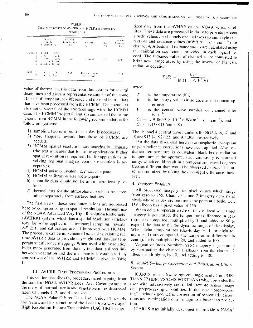
Fig. I. AYHRR (channel 4) thermal pattern of southeast Texas at about 2AM. April 25. 1983. Brightness proportional to relative equivalent black-body radiation temperature.
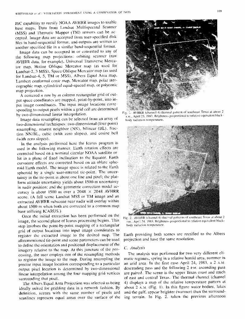
Fig. 2. AYHRR (channel 4) thermal patterns of southeast Texas at about 2PM .• April 24. 1983. Brightness proportional to relative equivalent black-body radiation temperature.
Earth providing both scenes are rectified to the Albersprojection and have the same resolution.
C. AnalysisThe analysis was performed for two very different cli-
matic regimes, spring in a relative humid area, summer inan arid area. In the first case April 24, 1983, a 2 AM.
descending pass and the following 2 P.M. ascending passare pai red. The scene is the upper Texas coast and muchof east and central Texas. The thermal channel (channel4) displays a map of the relative temperature pattern atabout 2 A.M. (Fig. I). In this figure water bodies, lakesand the gulf, appear brighter (warmer) than the surround-ing terrain. In Fig. 2, taken the previous afternoon

110IEEE TRANSACTlOT\S ON GEOSCIENCE AND REMOTE SENSING, VOL. UE-24. NO. I. JANUARY IlJ86
Fig, 3, AVHRR (channel 4) day-night thermal difference pattern, Bright-ness proportional to relative diflcrence,
(2 P,M,), a reversal of that pattern is shown, A subset ofthe pixels of each view was selected for processing Icarusby defining four corner points as shown by the boxes inthese figures. Note that the corners of the boxes are nearto but not necessarily at the same geographic position inthe two views. Using the satellite ephermeris data pro-vided in the header, Icarus was then used to register thetwo views to a geographic map base (in this example anAlbers Equal Area Projection was employed). Resamplingwas performed by using the nearest neighbor technique.A single tie-point was selected and the two views regis-tered and differenced.
The map of day-night temperature difference is shownin Fig. 3. Temperature differences in the lakes (R-12) andbays (T-23) are very small, of the order of 1°C. The forestto the north of Galveston Bay (Q-15) consisting of mixedpine and hardwood shows a modest 14°-lrc difference.The prairie to the upper left side of the figure (0-7) showsa difference of 20° -23°C and the bare soil prepared forplanting in the Brazos bottoms (0-10 to G-15) (ropelikebright area to left of figure) and the rice land lower right(W-19) show the greatest differences, 25°-28°C.
Paralleling the temperature difference pattern a mea-sure of vegetation was derived from the daylight pass bydifferencing (channel 2-channel 1) [2]. This difference isshown in Fig. 4. (The brighter the pixel the more vege-tated it is.) Here, the bare soil in the Brazos Bottoms andthe rice land appear very dark. Some major transportationarteries with their development appear in the vicinity ofHouston, bottom center right. Note that the registrationobtained between ascending and descending passesthrough ICARUS (Fig. 3) is degraded little if any fromthat obtained from the simultaneous view (Fig. 4). Com-parison of values of individual pixels in these figures sug-gests that for land surfaces higher values of vegetation in-
Fig, 4. Gray-McCrary vegetation index (AVHRR Channel 2-Channel I) atabout 21',\1., April 24, 1983, Brighlness propl1l1ional 10 relative vegeta-tion contribution.
Fig, 5, Vegctation index, north Texas and southwest Oklahoma, as ob.servcd at 2 P.M, Septcmber 3, IlJ83, White is highly vegetatcd, blacklittle vegetation. Clouds, mid-right and lower righL and lakes appear inblack,
dex are associated with lower values of temperaturedifference and vice versa as would be expected with theevapotranspiration of actively growing vegetation.
The second scene, depicted in Figs. 5~7, is north Texasand southwest Oklahoma during the late summer of 1983,For reference Oklahoma City is at X-6, Fort Worth at X-18, Lubbock at C- [3 and Amarillo at C-5. The vegetationindex shows high values along the eastern edge of theframe in Fig. 5, and also in the high plains between Lub-bock and Amarillo along the western edge. Patches of high
WHITEHEAD ef al.: VEGETATION ASSESSMENT USING A COMBINATION OF DATAIII
1 B
+ t
IV. CONCLUSIONS AND RECOMMENDATION
There appears to be significant and unique informationconcerning vegetation in thermal inertia data on this scale.The technology to study thermal inertia and its relation tovegetation cover on a coarse scale (1 plus km pixels) nowexists. The satellites to acquire the data are in place andare now providing data daily. The software and proce-dures are formulated and can be made available to inter-ested scientists. In performing this early study and in thedetailed follow-up now in progress we have found compli-cations in attempts to track the patterns described here in
values appear over the remainder of the scene but in gen-eral values are low indicating the poor state of vegetationin the unirrigated rangeland. Note for later discussion, thepattern of "lakes" in the vicinity of Wichita Falls P-B.
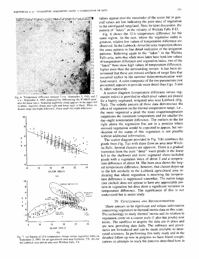
Fig. 6 shows the 12-h temperature difference for thesame region. To the east, where the vegetative index isgreatest, relative low values of temperature difference areobserved. In the Lubbock-Amarillo area inspection showsthe same pattern in fine detail indicative of the irrigationpatterns. Referring again to the "lakes" in the WichitaFalls area. note that while most lakes have both low valuesof temperature difference and vegetation index, two of the"lakes" here show high values of temperature difference,higher even than the surrounding terrain. It has been de-termined that these are instead artifacts of range fires thatoccurred earlier in the summer (telecommunication withland owner). A color composite of the two parameters (notpresented) appears to provide more detail than Figs. 5 and6, taken separately.
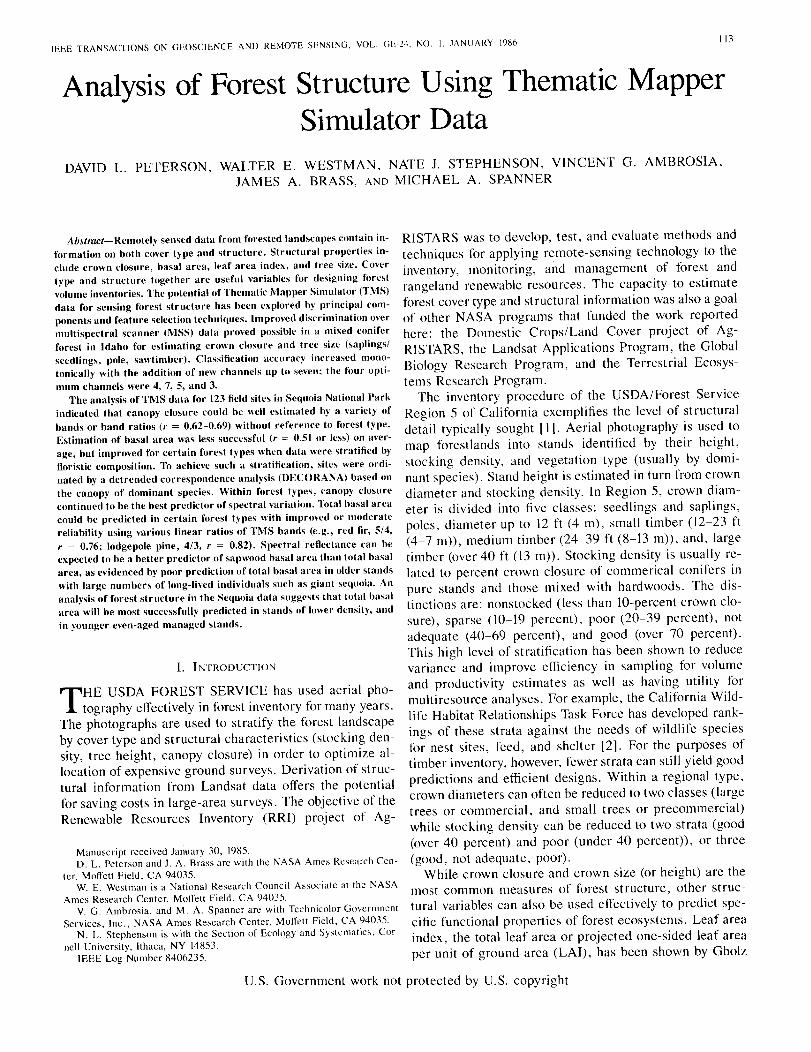
A scatter diagram (temperature difference versus veg-etation index) is provided in which pixel values are plottedfor a highly vegetated, irrigated area near Lubbock (Fig.7(a)). The orderly pattern of these data demonstrate theeffect of vegetation on the diurnal temperature range, i.e.,the more vegetated a pixel the more evapotranspirationsuppresses the maximum temperature and the smaller theday-night temperature difference. The outliers to the farright above the regression line are in a position wherestressed vegetation would be expected to appear, but ver-ification of the status of this vegetation is not possiblewithout additional information.
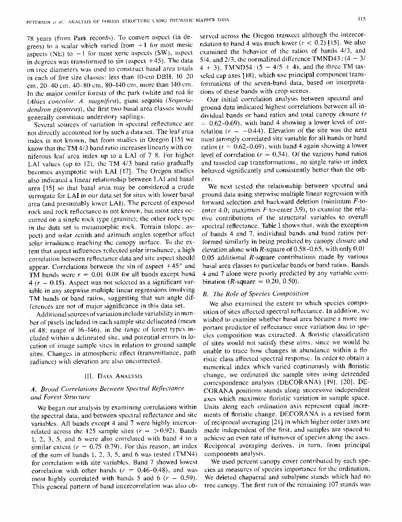
The scatter diagram provided in Fig. 7(b) combines thepixels from Fig. 7(a) with those from an area near Witch-ita Falls. Several clusters are apparent. There is a gradualtransition from the pure "deep" water pixels in the lowerleft to the shallower and more vegetated shore-includedpixels with a vegetation index of about 2 and a tempera-ture difference of about 14. The burn area shows the larg-est temperature difference, however, that cluster slopes upto the left similarly to the Lubbock agricultural area in-dicating that where vegetation is returning the tempera-ture difference is suppressed somewhat. The native range(not circled) does not appear to have any appreciable pat-tern in vegetation but does show a significant variation intemperature difference. The significance of this is notunderstood but is under study.
26
2422
1814
DEL'TEMf' (DEG.C)
18 28
DEL lUI' (DEG.Cl
(a)
18
16
-2
18
U 4
u
(b)
Fig. 7. (a) Pattern of 12-h temperature change versus vegetative index onSeptember 3, 1983, for an agricultural area near Lubbock, TX. (b) Forthe Lubbock area and an area near Witch ita Falls, TX.
'lAFig. 6. Temperature difference between 2 P.M., September 3, 1983, and 2
A.M., September 4, 1983, generated by differencing the ICARUS prod-ucts for those times. Scattered nighttime cloud appears in the upper leftin white. Daytime clouds mid-right and lower right in black. White in-dicates large day/night difference, black small day/night difference.

112IEEE TRANSACTIONS ON GEOSCIENCE AND REMOTE SENSING, VOL. GE-24, NO. I, JANUARY 1986
time. This is due in part to changes in atmospheric char-acteristics that affect the evapotranspiration rate and inpart to the difference in viewing geometry that affects thevegetation index. These problems are solvable and need tobe addressed before the full potential of this approach tovegetation condition assessment can be realized. The ap-plication of this technique to problems such as monitoringdrought and rangeland productivity changes should be at-tempted once these improvements are made,
REFERENCES
[I] J. A. Boatright and W. M. Bradley, "Image correction and registrationutility system," ICARUS Design Document, Lockheed Engrg. andManagement Services Co., 1985.
[2] T. I. Gray and D. G. McCrary, "AVHRR radiometer data estimationfor use in monitoring vegetation." in Extended Abstracts 15th Con!Agriculture and Meteorol., Amer. Meteorology Soc., 1981.
[3] R. D. Jackson, S. B. Idso, R. J. Reginato, and P. 1. Pinter, Jr., "Canopytemperature as a water stress indicator," Water Resour. Res., vol. 17,1981.
[4] K. B. Kidwell, NOM Polar Orbiter Data User's Guide, NOAA, NES-DIS, NCDC, SDSD, Washington, DC, 1983.
[5] J. C. Price, "Estimation of regional scale evapotranspiration throughanalysis of satellite thermal infrared data," IEEE Trans. Geosci. Re-mote Sensing, vol. GE-20, 1982.
[6] N. M. Short and L. M. Stuart, "The heat capacity mapping missionanthology," NASA SP-46.
Victor S. Whitehead received the B.A. degree inphysies and math from Baylor University, the M.S.degree in meteorology from Texas A & M Uni-versity, College Station, and the Ph.D. degree inengineering sciences from the University of Okla-homa.
Sinee 1968, he has been employed at the NASAJohnson Space Center, Houston, TX, in a varietyof Earth Observations Program and Remote Sens-ing Program Assignments, including LACIE andAgRISTARS.
*William R. Johnson received the B.S. degree in meteorology from the Uni-versity of Chicago and the M. S. degree in meteorology from Florida StateUniversity.
He is a Principal Scientist at Lockheed Engineering and ManagementServiees Company, Houston, TX. His current assignment involves deter-mination of information content for land-inventory tasks. Formerly, heserved as a Meteorology Consultant during Skylab missions.
*James A. Boatwright received the B.S. degree in physics from Texas A&MUniversity, College Station, in 1965.
He is currently a Systems Engineer with Lockheed Engineering andManagement Services Company, Houston, TX. He has contributed to thedevelopment of several Earth Resources image-processing systems for theNASA Johnson Space Center since 1965. The ICARUS system is the latestof these, and incorporates his "orbiting seanner" map projection to rectifyNOAA AVHRR (or similar) images to the Earth's surface.
IEEE TRANSACTIONS ON GEOSCIENCE AND REMOTE SENSING, VOL. GE-24, NO. 1. JANUARY 1986113
Analysis of Forest Structure Using Thematic MapperSimulator Data
DAVID L. PETERSON, WALTER E. WESTMAN, NATE 1. STEPHENSON, VINCENT G, AMBROSIA,JAMES A. BRASS, AND MICHAEL A, SPANNER
Abstmct-Remotely sensed data from forested landscapes contain in-formation on both cover type and structure. Structural properties in-clude crown closure, basal area, leaf area index, and tree size. Covertype and structure together are useful variables for designing forestvolume inventories. The potential of Thematic Mapper Simulator (TMSldata for sensing forest structure has been explored by principal com-ponents and feature selection techniques. Improved discrimination overmultispectral scanner (MSS) data proved possible in a mixed coniferforest in Idaho for estimating crown closure and tree size (saplings!seedlings, pole, sawtimber). Classification accuracy increased mono-tonically with the addition of new channels up to seven; the four opti-mum channels were 4, 7, 5, and 3.
The analysis of TMS data for 123 field sites in Sequoia National Parkindicated that canopy closure could be well estimated by a variety ofbands or band ratios (r = 0.62-0.69) without reference to forest type.Estimation of basal area was less successful (r = 0.51 or less) on aver-age, but improved for certain forest types when data were stratified byfloristic composition. To achieve such a stratification, sites were ordi-nated by a detrended correspondence analysis (DECORAC'lA) based onthe canopy of dominant species. Within forest types, canopy closurecontinued to be the best predictor of spectral variation. Total basal areacould be predicted in certain forest types with improved or moderatereliability using various linear ratios of TMS bands (e.g., red fir, 5/4,r = 0.76; lodgepole pine, 4/3, r = 0.82). Spectral reflectance can beexpected to be a better predictor of sapwood basal area than total basalarea, as evidenced by poor prediction of total basal area in older standswith large numbers of long-lived individuals such as giant sequoia. Ananalysis of forest structure in the Sequoia data suggests that total basalarea will be most successfully predicted in stands of lower density, andin younger even-aged managed stands.
L INTRODUCTION
THE USDA FOREST SERVICE has used aerial pho-tography effectively in forest inventory for many years,
The photographs are used to stratify the forest landscapeby cover type and structural characteristics (stocking den-sity, tree height, canopy closure) in order to optimize al-location of expensive ground surveys, Derivation of struc-tural information from Landsat data offers the potentialfor saving costs in large-area surveys. The objective of theRenewable Resources Inventory (RRI) project of Ag-
Manuscript reccived January 30, 1985.D. L. Peterson and J. A. Brass are with the NASA Ames Research Cen-
ter. Moffett Field, CA 94035.W. E. Westman is a National Research Council Associate at the NASA
Ames Research Center, Moffett Field, CA 94035.V. G, Ambrosia, and M. A. Spanner are with Technicolor Government
Services, Inc., NASA Ames Research Center, Moffett Field, CA 94035.N. L. Stephenson is with the Section of Ecology and Systematics, Cor-
nell University, Ithaca, NY 14853.IEEE Log Numbcr 8406235.
RISTARS was to develop, test, and evaluate methods andtechniques for applying remote-sensing technology to theinventory, monitoring, and management of forest andrangeland renewable resources. The capacity to estimateforest cover type and structural information was also a goalof other NASA programs that funded the work reportedhere: the Domestic Crops/Land Cover project of Ag-RISTARS, the Landsat Applications Program, the GlobalBiology Research Program, and the Terrestrial Ecosys-tems Research Program.
The inventory procedure of the USDA/Forest ServiceRegion 5 of California exemplifies the level of structuraldetail typically sought [I]. Aerial photography is used tomap forestlands into stands identified by their height,stocking density, and vegetation type (usually by domi-nant species). Stand height is estimated in turn from crowndiameter and stocking density. In Region 5, crown diam-eter is divided into five classes: seedlings and saplings,poles. diameter up to 12 ft (4 m), small timber (12-23 ft(4-7 m)), medium timber (24-39 ft (8-13 m)), and, largetimber (over 40 ft (13 m)). Stocking density is usually re-lated to percent crown closure of commerical conifers inpure stands and those mixed with hardwoods. The dis-tinctions are: nonstocked (less than 10-percent crown clo-sure), sparse (10-19 percent), poor (20-39 percent), notadequate (40-69 percent), and good (over 70 percent).This high level of stratification has been shown to reducevariance and improve efficiency in sampling for volumeand productivity estimates as well as having utility formulti resource analyses. For example, the California Wild-life Habitat Relationships Task Force has developed rank-ings of these strata against the needs of wildlife speciesfor nest sites, feed, and shelter [2]. For the purposes oftimber inventory, however, fewer strata can still yield goodpredictions and efficient designs. Within a regional type,crown diameters can often be reduced to two classes (largetrees or commercial, and small trees or precommercial)while stocking density can be reduced to two strata (good(over 40 percent) and poor (under 40 percent)). or three(good, not adequate, poor).
While crown closure and crown size (or height) are themost common measures of forest structure, other struc-tural variables can also be used effectively to predict spe-cific functional properties of forest ecosystems. Leaf areaindex, the total leaf area or projected one-sided leaf areaper unit of ground area (LAI), has been shown by Gholz
U.S. Government work not protected by U.S. copyright

114IEEE TRANSACTIONS ON GEOSCIENCE ;\1\0 REMOTE SENSING. VOL. GE-24. :-.10. I, JANUARY 19X6
[4] to be an effective predictor of aboveground net primaryproductivity (NPP). The prediction of NPP was obtainedfor temperature coniferous forests of the Pacific North-west having a one-sided LAI range from one to twenty.Leaf area index is not being used to predict growth by theForest Service as yet, probably due to the difficulty inmeasuring LAI over large regions. Instead, the strata al-ready described are used with yield tables to derive growthestimates. Our own efforts to estimate leaf area index byremote sensing are cited below.
Earlier experience with Landsat MSS data [5]-[ 12J ledus to develop the hypothesis that the variance in a remote-sensing image of a forested area will be due as much tovariation in structural properties of communities (crownclosure, tree size, tree spacing, leaf area) as to variationsin species klbundance and cover type. Indeed, the "noise"of forest structure can contribute to the loss of classifica-tion accuracy 113[. As the spatial resolution of sensors isincreased from 60 to 30 m, there should be an increase invariance as the resolution size approaches the natural fre-quency of canopy structural characteristics, such as crowndiameter. Therefore, Thematic Mapper data might be ex-pected to contain increased structural information at theloss of cover type classification accuracy. For timber vol-ume estimation, this is an acceptable, perhaps preferred,tradeoff as structural properties are more closely associ-ated with functional variables like net primary productiv-ity and state variables like volume.
II. SIMULATED THEMATIC MAPPER ANALYSES
A. Forest Structure in Clearwater National Forest,Idaho
A region from the Clearwater National Forest in north-ern Idaho was chosen for analysis in the Renewable Re-sources Inventory program of AgRISTARS to evaluatethe capabilities of the Thematic Mapper. Simulated TM(TMS) data were acquired for this mixed-conifer in-tensely-managed forest. A complete range of regrowthconditions exists here. Similar results arose from both aprincipal components analysis and a Monte Carlo simu-lation selecting features (channels) that optimize for ac-curacy of classification of a training data set. A classifi-cation scheme and appropriate training sites were selectedpurposely to highlight structural features (good/poorstocking; seedlings/saplings, poles, sawtimber) as well asthe harvesting patterns and other cover conditions in thearea. Channel 4 (760-900 nm), channel 7 (thermal:10 400-12 500 nm), channel 5 (1530-1730 nm), andchannel 3 (630-690 nm) were the optimal bands, in thatorder, to explain scene variance. Training site statisticswere used to classify the scene by maximum likelihoodtechniques. Classification accuracy for seven-channel 30-m TMS data were found to be superior to a four optimumchannel (3, 4, 5, 7) 30-m data set. These in turn consist-ent~y outperformed a simulated three-channel MSS dataset. The Monte Carlo technique showed that the classi-fication accuracy increased monotonically as each new
channel up to the full seven was added to the analysis.Virtually no stand dimensional data were available for thissite. Thus further analyses to establish the particularst ructural or other variable contributing most strongly tothese results were not possible 114]. This study laid thegroundwork for further research at two new locations forwhich carefully measured structural properties were ob-tained. Results of a study in Oregon have been reportedelsewhere 115]; we discuss below our most recent effortsin the montane forests of California.
B. Forest Structure in Sequoia National Park,Cal~fornia
Sequoia National Park, in the southern Sierra Nevada,represents a particularly complex vegetation mosaic, rang-ing from chaparral shrubland and broad-leaved forest tomontane and subalpine coniferous forest stands. Most ofthe vegetation has not been logged in the past 95 years,resulting in mixed-age mixed-species stands characteristicof natural, rather than heavily managed, forest land-scapes. Airborne Thematic Mapper (ATM) data were ob-tained over ]20 O.I-ha and 3 0.02-ha sites for whichground data were available in the Park. The ground datawere collected by N. L. Stephenson during 1982-1983.The data included information on species composition inthe canopy, canopy closure, and basal area by species. Wesought to determine the extent to which the forest struc-tural variables influenced, and in turn could be predictedby, the spectral data.
C. Collection and Refinement qf Spectral Data
ATM data (flight 83-164) were collected on September2, 1983, between 1l :40 AM. and 12: 16 PM. (solar noon).The Daedalus Airborne Thematic Mapper (ATM) wasflown aboard a NASA U-2C aircraft at 19 800 m, alongfour N-S trending flight lines of 16.6-km swath width. Thescan angle of the sensor was 430 with 716 pixels per scanline. Ground resolution with an IFOV of 1.3 mrad at themean Park elevation of 2300 m was 23.2 m. The ATMacquires twelve channels of information of which the sevensimulated TM bands were used: channel I (450-520 nm),2 (520-600 nm), 3 (630-690 nm), 4 (760-900 nm), 5(1530-1730 nm), 6 (2100-2300 nm), and 7 (10.4-12.5 jLm).
Because the sun angle was not in the plane of the flightline, the proportion of reflected radiation coming from theground and from atmospheric backscattering changed withscan angle. These limb brightening conditions were cor-rected by a column-averaging program in which valuesaway from the scanner nadir were corrected for averagedeviation from scene nadir values [16].
D. Collection and Re,finement of Ground Data
The following information was available for each of the123 sites for which spectral data were collected: elevation,slope, aspect, total canopy closure (percent), percent ofcanopy dominated by each species, abundance of domi-nant tree species in each of 12 diameter at breast height(DBH) classes, and date of most recent fire within the past
PETERSON 1'1 al .. ANALYSIS OF FOREST STRUCTURE USING THEMATiC MAPPER DATA /15
78 years (from Park records). To convert aspect (in de-grees) to a scalar which varied from + I for most mesicaspects (NE) to - I for most xeric aspects (SW), aspectin degrees was transformed to sin (aspect +45). The dataon tree diameters was used to construct basal area totalsin each of five size classes: less than lO-cm DBH, lO-20cm, 20-40 cm, 40-80 cm, 80-140 cm, more than 140 cm.In the major conifer forests of the park (white and red fir(Abies concolor, A. magnifica), giant sequoia (Sequoia-dendron gigantea)), the first two basal area classes wouldgenerally constitute understory saplings.
Several sources of variation in spectral reflectance arenot directly accounted for by such a data set. The leaf areaindex is not known, but from studies in Oregon [15] weknow that the TM 4/3 band ratio increases linearly with co-niferous leaf area index up to a LAI of 7-8. For higherLAI values (up to 12), the TM 4/3 band ratio graduallybecomes asymptotic with LAI [17]. The Oregon studiesalso indicated a linear relationship between LAI and basalarea [15] so that basal area may be considered a crudesurrogate for LAI in our data set for sites with lower basalarea (and presumably lower LAI). The percent of exposedrock and rock reflectance is not known, but most sites oc-curred on a single rock type (granite); the other rock typein the data set is metamorphic rock. Terrain (slope, as-pect) and solar zenith and azimuth angles together affectsolar irradiance reaching the canopy surface. To the ex-tent that aspect influences reflected solar irradiance, a highcorrelation between reflectance data and site aspect shouldappear. Correlations between the sin of aspect + 45 0 andTM bands were r = 0.01-0.08 for all bands except band4 (r = 0.15). Aspect was not selected as a significant var-iable in any stepwise multiple linear regressions involvingTM bands or band ratios, suggesting that sun angle dif-ferences are not of major significance in this data set.
Additional sources of variation include variability in num-ber of pixels included in each sample site delineated (meanof 48; range of 16-146), in the range of forest types in-cluded within a delineated site, and potential errors in lo-cation of image sample sites in relation to ground samplesites. Changes in atmospheric effect (transmittance, pathradiance) with elevation are also uncorrected.
III. DATAANALYSIS
A. Broad Correlations Between Spectral Reflectanceand Forest Structure
We began our analysis by examining correlations withinthe spectral data, and between spectral reflectance and sitevariables. All bands except 4 and 7 were highly intercor-related across the 125 sample sites (r = >0.92). Bands1, 2, 3, 5, and 6 were also correlated with band 4 to asimilar extent (r = 0.75-0.79). For this reason, an indexof the sum of bands 1, 2, 3, 5, and 6 was tested (TMN4)for correlation with site variables. Band 7 showed lowestcorrelation with other bands (r = 0.46-0.48), and wasmost highly correlated with bands 5 and 6 (r = 0.59).This general pattern of band intercorrelation was also ob-
served across the Oregon transect although the intercor-relation to band 4 was much lower (r < 0.2) [15]. We alsoexamined the behavior of the ratios of bands 4/3, and5/4, and 2/3, the normalized difference TMND43 : (4 - 3/4 + 3), TMND54: (5 - 4/5 + 4), and the three TM tas-seled cap axes [18], which use principal component trans-formations of the seven-band data, based on interpreta-tions of these bands with crop scenes.
Our initial correlation analysis between spectral andground data indicated highest correlations between all in-dividual bands or band ratios and total canopy closure (r= 0.62-0.69), with band 4 showing a lower level of cor-relation (r = - 0.44). Elevation of the site was the nextmost strongly correlated site variable for all bands or bandratios (r = 0.62-0.69), with band 4 again showing a lowerlevel of correlation (r = 0.34). Of the various band ratiosand tasseled cap transformations, no single ratio or indexbehaved significantly and consistently better than the oth-ers.
We next tested the relationship between spectral andground data using stepwise multiple linear regression withforward selection and backward deletion (minimum F-to-enter 4.0; maximum F-to-enter 3.9), to examine the rela-tive contributions of the structural variables to overallspectral reflectance. Table I shows that, with the exceptionof bands 4 and 7, individual bands and band ratios per-formed similarly in being predicted by canopy closure andelevation alone with R-square of 0.58-0.65, with only 0.01-0.05 additional R-square contributions made by variousbasal area classes to particular bands or band ratios. Bands4 and 7 alone were poorly predicted by any variable com-bination (R-square = 0.20, 0.50).
B. The Role of Species CompositionWe also examined the extent to which species compo-
sition of sites affected spectral reflectance. In addition, wewished to examine whether basal area became a more im-portant predictor of reflectance once variation due to spe-cies composition was extracted. A floristic classificationof sites would not satisfy these aims, since we would beunable to trace how changes in abundance within a flo-ristic class affected spectral response. In order to obtain anumerical index which varied continuously with floristicchange, we ordinated the sample sites using detrendedcorrespondence analysis (DECORANA) [19], [20]. DE-CORANA positions stands along successive independentaxes which maximize floristic variation in sample space.Units along each ordination axis represent equal incre-ments of floristic change. DECORANA is a revised formof reciprocal averaging [21] in which higher order axes aremade independent of the first, and samples are spaced toachieve an even rate of turnover of species along the axes.Reciprocal averaging derives, in turn, from principalcomponents analysis.
We used percent canopy cover contributed by each spe-cies as measures of species importance for the ordination.We deleted chaparral and subalpine stands which had notree canopy. The first run of the remaining lO7 stands was
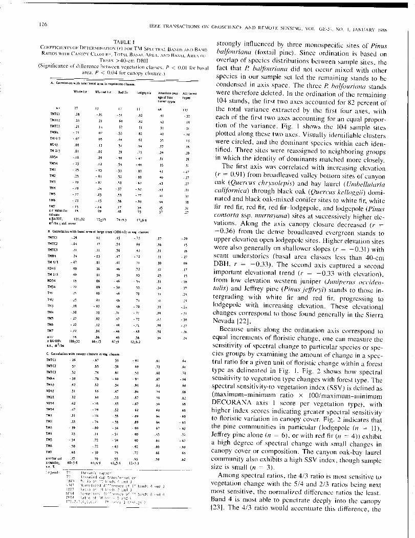
116IEEE TRANSACTIONS ON GEOSCIENCE AND REMOTE SENSI'JG, VOL. GE-24, NO. I, JANUARY 19R6
A. Cot"reli.tion with totil! basal ou-ea in vegetation dUlles.
While fir Wh/red [if Red fir Lodgepole AbliOlute ltVer- All forest
age of four typesrorest tYP85
Legend: Tr1 The'lldtic Illap:Jer
TC Tasse1('d truns~orrlidtionT\14.'3 Ra t jrJ of 4 and 3WJ43 NCYTIalizcd d'ffer('n,~e of bands 4 and 3T,"123 Ra t'i 0 of :-n [:,'1'ld5 2 Clno 3ND54 'lorr:Ii',lized di ffC:'rel~ce of Tn cdnds ;'nd 4TM5u. :;;iltio of TM bJrds 5 and 4HH,2,3,4,5,6,7 TV bi',nds 1 thl"oJ]h 7
strongly influenced by three monospecific sites of Pinushalfouriana (foxtail pine). Since ordination is based onoverlap of species distributions between sample sites, thefact that P. halfouriana did not occur mixed with otherspecies in our sample set led the remaining stands to becondensed in axis space. The three P. ha~louriana standswere therefore deleted. In the ordination of the remaining104 stands, the first two axes accounted for 82 percent ofthe total variance extracted by the first four axes. witheach of the first two axes accounting for an equal propor-tion of the variance. Fig. I shows the 104 sample sitesplotted along these two axes. Visually identifiable clusterswere circled, and the dominant species within each iden-tified. Three sites were reassigned to neighboring groupsin which the identity of dominants matched more closely.
The first axis was correlated with increasing elevation(r = 0.91) from broadleaved valley bottom sites of canyonoak (Quercus chrysolepis) and bay laurel (Umhel/ulariacalifornica) through black oak (Quercus kelloggii) domi-nated and black oak-mixed conifer sites to white fir, whitefir-red fir, red fir, red fir-lodgepole, and lodgepole (Pinuscontorta ssp. murrayana) sites at successively higher ele-vations. Along the axis canopy closure decreased (r =-0.36) from the dense broad leaved evergreen stands toupper elevation open lodgepole sites. Higher elevation siteswere also generally on shallower slopes (r = - 0.31) withscant understories (basal area classes less than 40-cmDBH, r = -0.33). The second axis captured a secondimportant elevational trend (r = -0.33 with elevation),from low elevation western juniper (Juniperus occiden-talis) and Jeffrey pine (Pinus jetlreyi) stands to those in-tergrading with white fir and red fir, progressing tolodgepole with increasing elevation. These elevationalchanges correspond to those found generally in the SierraNevada [22].
Because units along the ordination axis correspond toequal increments of floristic change, one can measure thesensitivity of spectral change to particular species or spe-cies groups by examining the amount of change in a spec-tral ratio for a given unit of floristic change within a foresttype as delineated in Fig. I. Fig. 2 shows how spectralsensitivity to vegetation type changes with forest type. Thespectral sensitivity-to-vegetation index (SSV) is defined as(maximum-minimum ratio X 100/maximum-minimumDECORANA axis I score per vegetation type), withhigher index scores indicating greater spectral sensitivityto floristic variation in canopy cover. Fig. 2 indicates thatthe pine communities in particular (lodgepole (n = II),Jeffrey pine alone (n = 6), or with red fir (n = 4)) exhibita high degree of spectral change with small changes incanopy cover or composition. The canyon oak-bay laurelcommunity also exhibits a high SSV index, though samplesize is small (n = 3),
Among spectral ratios, the 4/3 ratio is most sensitive tovegetation change with the 5/4 and 2/3 ratios being nextmost sensitive, the normalized difference ratios the least.Band 4 is most able to penetrate deeply into the canopy[23 J. The 4/3 ratio would accentuate this difference, the
2\
.24
103
-.32
19
31
- 30
I)
18
.20
-.29
-31
- 27
- 27
- 27
-31
-)3
-30
-3127
- 29
.15
28
-27
09
17
15
- 2b
- 27
-.31
-.30
- 27
-.28
.2<
-M
.bl
.70
- bb
.60
66
b2
b8
-68
-,60
-.bl
- b3
- 32
-.b7
- b9
- b5
b2
<2
31
42
35
)7
29
31
33
.1H
.2537
Al
<J
40
40
A)
37
36
.31
31
3032
25
31
.3'y~
\b
bl
35
.39
.)7
.39
30
J4
.72
.bO
.b7
.b3
70
58
58
60
M
M
67
A5
.M
.b9
bO
59
.82
31
-.82
82
8<
73
II
-.82
·47
-.44
-.83
- 83
- 82
71
-.72
b9
A2
-.72
71
.72
63
- 5'-53
70
-,70
-.71
-72
-.71
-.18
5b12~Jd
17
-51
60
57
-.53
.H
.52
39
- 50
-.5'
-.53
- 52
-.53
- '5
5'50
-.47
.41
.'8
3b
-.46
-.50
,b
4b
- .6
-31
-<7
-.07
05
.13
.02
- 09
-12
- 03
- 01
21 - 37 -.82
-.0' - 'B -.77
- 15 - 5b -.80
-.14 .17 .)409 48 73
13
-.01
21
14
07
02
17
II
-03
01
08
- 01
-.Ob
- 09
00
.01
- 03
.23
-.02
-12
-.04
06bb~15
27
-.28
-OJ21
-.21
-.07
.00
-01
- 18
-23
-25
-.25
- 19
TMTCI
TMTC2
TMTCl
TMN4
TM4/3
N043
TM 213
ND5'
TM5'
TMI
TM2
TM3
1M4 -.2~
TM~ -,27
TMb -.23
1M? -.15xr-valuelor .18columnxBATOT. 121.32m2/hl.!.. std. error -
B. Correlation with basal area of large trees (08H>40' in veg. classes
TM2 l~
TM3 -.19
TM. -.30
TM5 - 27
TMb -22
TM7 -.22
TMTCI - 29
TMTC2 -.04
TMTC3 .21
TMN4 - 24
TM 4/3 -.07
ND13 .00
1M 213 .00
ND5' - 18
TM54 -.22
1M! 2~
x/rl 18x BA40P. I 08~335.8., m2iblC. Cocrelation with canopy closure in Vet- c1uses
TMTCI - 26
TMTC2 57
TMTC3 52
TMN4 -.39
TMi3 .42
ND43 51
TM23 32
NOH - 42
TM5<i - 47
TMJ -.31
TM2 -.33
TM3 -_39
TM4 23
TM5 -.3'
TM6 -.50
TM7 -.63
-.b7 -59 - 91
.85 58 89
.74 61 .51
-76 -60 -91
82 .H .94
.86 .7 .9'
80 .33 .87
-.78 -.15 -.67
- 79 - 52 -.b2
-.78 ~.~8 -89
-7. ·.58 -.89
-.80 - 58 - 90
.14 - 51 - 90
- 72 - 59 90
-.72 -.b3 -.92
- 30 - 75 -72
xh/for col 37 .70 55 85x canclo.!- 60.:!.,3.6 41~"9 41.0.<1 t2.:!..3.3
-•• -., %~--~~_. __ .__ .__..._--~~-~_ .._------~-~~~-
TABLE ICOEFFICIENTS OF DETERMINATIOI\ (r) FOR TM SPECTRAL BA:'ms AI\IJ BAND
RATIOS WITH CANOPY CUlSLTRF. TOTAL BASAL AREA. AI\IJ BASAL. ARIA 01'
TREES >40-cm DBH
(Significance of ditlcrence between vegetation classes, P < O.Ot klr basalarea. P < 0.04 for canopy closure.)
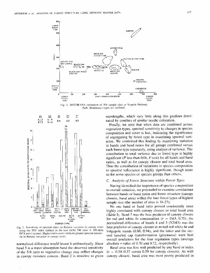
PETERSON et al .. ANALYSIS OF FOREST STRL'CTURE USING THEMATIC MAPPER DATA 117
600
LOWERELEVA-
TION
500JUNIP~
400
N
~ 300
"
JEFFREY PINE
WHITE FIR- QJEFFREY PINE
O CSREDFIR-JEFFREY PINE
CANYON OAK
BAY LAUREL BLACK OAK ••• ~:.
200 ~/~~ coBLACK OAK-MIXED WHITE FIR WHITE- FIR~ ~.:. RED FIR
CONIFER RED FIR •
100
HIGHERELEVA·TION
LODGEPOLE
LOWERELEVA
TlON
100 200 300 400 500AXIS 1 ORDINATION SCORE
600 700 BOO
HIGHERELEVATIQN
Fig. 1. DECORANA ordination of ]04 sample sites at Sequoia NationalPark. Dominance types arc outlined.
8
14[;J
oCANYON I OAK - I WHITE I LODGE IRED FIR -I ALLOAK - BAY MIXED FIR - POLE JEFFREY TYPESLAUREl CONIFER RED FIR PINE PINE COMBINED
BLACK WHITE RED FIR WHITE JEFFREYOAK FIR FIR - PINE
JEFFREY
PINE
FOREST TYPE
Fig. 2. Sensitivity of spectral ratios to floristic variation in canopy coverusing the SSV index defined in the text (delta TM ratio x IOO/deltaDCA axis 1 scores). Higher index scores indicate greater spectral sensitiv-ity to floristic variation in canopy cover.
wavelengths, which vary little along this gradient domi-nated by conifers of similar needle coloration.
Finally, we note that when data are combined acrossvegetation types, spectral sensitivity to changes in speciescomposition and cover is lost, indicating the significanceof segregating by forest type in examining spectral vari-ation. We confirmed this finding by examining variationin bands and band ratios for all groups combined versuseach forest type separately, using analysis of variance. Thecontribution to total variance due to forest type is highlysignificant (P less than 0.01, F-test) for all bands and bandratios, as well as for canopy closure and total basal area.Thus the contribution of variations in species compositionto spectral reflectance is highly significant, though moreso for some species or species groups than others.
C. Analysis of Forest Structure within Forest TypesHaving identified the importance of species composition
to overall variation, we proceeded to examine correlationsbetween bands or band ratios and forest structure (canopyclosure, basal area) within the four forest types of highestsample size (the number of sites is 11-27).
No one band or band ratio proved consistently mosthighly correlated with canopy closure or total basal area(Table I). Band 7 was the best predictor of canopy closurefor red and white fir communities (r = 0.63, 0.75); thenormalized difference of bands 4 and 3 (ND43) was thebest predictor of canopy closure in mixed red-white fir andlodgepole stands (0.86, 0.94), and the latter and the sec-ond tasseled cap transformation (greenness) were bestoverall predictors for the four vegetation types (averageabsolute r-value of 0.70 and 0.72, respectively).
Basal area was less well predicted by any band or index(r = 0.34-0.37 versus 0.59 for canopy closure). As withcanopy closure, basal area was most poorly predicted in
[]
4/3
[';J I2l [l] []4-3 5-4 5/4 2/3I 4+3 5+4
~
,i
I;;-;
I
millI~
~~
xUJ 7Clzzoi= 6<t>-UJ
"UJ
~ 5o>;->>-> 4i=iiizUJrn-' 3<ta:>-uUJg; 2
normalized difference would lessen it arithmetically. Sinceband 5 is a water absorption band the observed sensitivityof the 5/4 ratio to vegetative change may reflect changesin canopy moisture content. Band 2 is sensitive to green
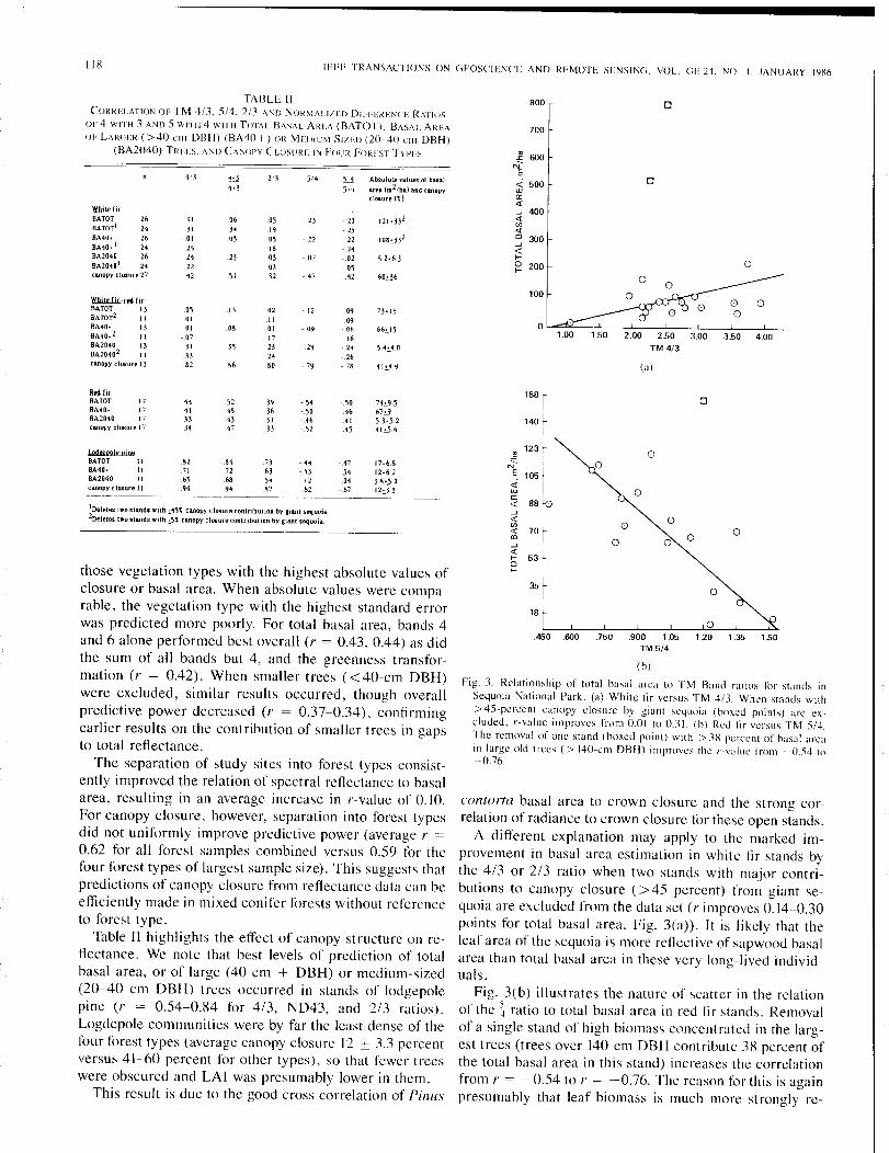
118 IEEE TRANSACTIONS ON GEOSCIENCE AND REMOTE SENSI!\G, VOL GE24. NO.1. JANUARY 1986
(b)
Fig. 3. Relationship of total basal arca to TM Band ralios lilr stands inSequoia National Park. (a) White fir vcrsus TM 413. When stands with> 45-pcrcent canopy closure by giant scquoia (boxed points) arc ex-cluded, r-value improves from 0.01 to O.3!. (h) Red fir versus TM 5/4.Thc rcmoval of onc stand (boxed point) with > 3~ perccnt of basal areain largc old trces (> 140-cm DBH) improves thc r-value from -0.54 to-0.76.
contorta basal area to crown closure and the strong cor-relation of radiance to crown closure for these open stands,
A different explanation may apply to the marked im-provement in basal area estimation in white fir stands bythe 4/3 or 2/3 ratio when two stands with major contri-butions to canopy closure (> 45 percent) from giant se-quoia are excluded from the data set (r improves 0,14-0.30points for total basal area, Fig, 3(a», It is likely that theleaf area of the sequoia is more reflective of sapwood basalarea than total basal area in these very long-lived individ-uals,
Fig, 3(b) illustrates the nature of scatter in the relationof the ~ ratio to total basal area in red fir stands, Removalof a single stand of high biomass concentrated in the larg-est trees (trees over 140-cm DBH contribute 38 percent ofthe total basal area in this stand) increases the correlationfrom r = -0,54 to r = -0,76, The reason for this is againpresumably that leaf biomass is much more strongly re-
1.35 1.50.450 .600 .750 .900 1.05TM 5/4
800 0
7eo
~ 600~N
Er
<t 500wa::<t..J 400<tU)«on 300..J«I-
00 200I-
00
1000 00
01.00 1.50 2.00 2.50 3.00 3.50 4.00
TM 4/3
(a)
158 r.
140
~ 123~
N
E<t'wa::«..J«U)
«on..J«I-0I-
4/3 U 2/3 ')/4 U Absolute values or bual4-3 5" a.rea Im2/hl.l and canopy
closure (1)
White fir121~J32BA TOT 26 01 06 .05 23 ~23
BATor I ,. 31 J4 19 .2)BAtiO. 26 -.01 01 0' -22 -22 IOS~332BA-"O.I ,. 2S 18 -24BA2040 26 24 .23 03 -.07 - 02 82,63BA20iOI 24 22 03 05canopy closure 27 42 51 32 -.47 - 42 60;,3,6
WbileJir-red firBATOT 13 05 13 02 .Il - 09 73:!:J5SA TOT2 II .01 -II 09BA40. 13 01 08 -01 ~.O9 - 06 66,11BA40.2 II - 07 - 17 16BA20iO 13 31 31 23 - 29 -24 '.4:.4.0BA20402 11 33 .24 - 26canopy closure 13 82 86 80 - 79 - 78 41 •.49
Il&l.ir.BATOT 17 4' .52 39 oj; - 50 74,95BA40· 17 41 48 36 '.50 - 46 67,9BA2040 17 33 43 31 - 46 - 41 53-52canopy closure 17 34 47 33 -52 -45 41-54
Lodlleoole DineBATOT 11 .82 84 .73 -<4 -.47 17,6.8BA40. 11 71 72 63 - 53 -54 12,6.2BAlOiO 11 65 68 j; 12 .04 38-5.0canopy closure I J 94 94 87 - 62 -.67 12033--------------_.-
IOeletes two stands with £.451 canopy closure contribution by giant SeqUOiL2Deletes two stands wilh 2,5% clUlopy closure cOfluiburion by giant seqUOia.
TABLE IICORREl.ATlON OF TM 4/3, 5/4, 2/3 Ar\O NOR\1AI.I/FO D1HTRENCE RATIOS
OF 4 WITH 3 AND 5 WITH 4 WITH TOTAL BASAL ARh\ (BATCH). BASAL AREA
01" LAR(;ER (> 40 cm DB H) (BA40+) OR MEIlIUM-SII.EIJ (20-40 cm DBH)
(8A2040) TRH:S. A'IIJ CA'IOI'Y CLOSURE ,'< FOUR FORFST TYPFS
those vegetation types with the highest absolute values ofclosure or basal area, When absolute values were compa-rable, the vegetation type with the highest standard errorwas predicted more poorly, For total basal area, bands 4and 6 alone performed best overall (r = 0,43, 0,44) as didthe sum of all bands but 4, and the greenness transfor-mation (r = 0,42), When smaller trees «40-cm DBH)were excluded, similar results occurred, though overallpredictive power decreased (r = 0.37-0,34), confirmingearlier results on the contribution of smaller trees in gapsto total reflectance,
The separation of study sites into forest types consist-ently improved the relation of spectral reflectance to basalarea, resulting in an average increase in r-value of 0,10,For canopy closure, however, separation into forest typesdid not uniformly improve predictive power (average r =
0,62 for all forest samples combined versus 0,59 for thefour forest types of largest sample size). This suggests thatpredictions of canopy closure from reflectance data can beefficiently made in mixed conifer forests without referenceto forest type,
Table II highlights the effect of canopy structure on re-flectance, We note that best levels of prediction of totalbasal area, or of large (40 cm + DBH) or medium-sized(20-40 cm DB H) trees occurred in stands of lodgepolepine (r = 0,54-0,84 for 4/3, ND43, and 2/3 ratios),Logdepole communities were by far the least dense of thefour forest types (average canopy closure 12 ± 3,3 percentversus 41-60 percent for other types), so that fewer treeswere obscured and LAl was presumably lower in them.
This result is due to the good cross correlation of Pinus
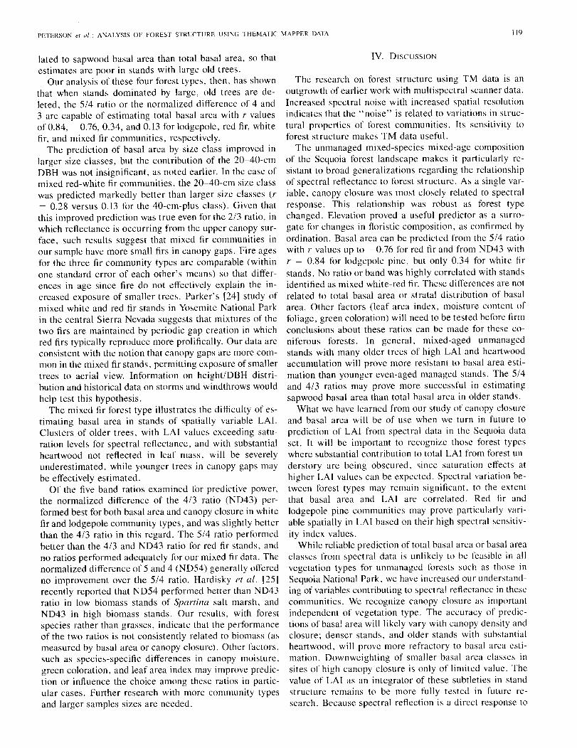
PETERSON et al.: ANALYSIS OF FOREST STRUCTURE USIl\G THEMATIC YlAPPER DATA 119
lated to sapwood basal area than total basal area, so thatestimates are poor in stands with large old trees.
Our analysis of these four forest types, then, has shownthat when stands dominated by large, old trees are de-leted, the 5/4 ratio or the normalized difference of 4 and3 are capable of estimating total basal area with r valuesof 0.84, -0.76,0.34, and 0.13 for lodgepole, red fir, whitefir, and mixed fir communities, respectively.
The prediction of basal area by size class improved inlarger size classes, but the contribution of the 20-40-cmDBH was not insignificant, as noted earlier. In the case ofmixed red-white fir communities, the 20-40-cm size classwas predicted markedly better than larger size classes (r= 0.28 versus 0.13 for the 40-cm-plus class). Given thatthis improved prediction was true even for the 2/3 ratio, inwhich reflectance is occurring from the upper canopy sur-face, such results suggest that mixed fir communities inour sample have more small firs in canopy gaps. Fire agesfor the three fir community types are comparable (withinone standard error of each other's means) so that differ-ences in age since fire do not effectively explain the in-creased exposure of smaller trees. Parker's [24] study ofmixed white and red fir stands in Yosemite National Parkin the central Sierra Nevada suggests that mixtures of thetwo firs are maintained by periodic gap creation in whichred firs typically reproduce more prolifically. Our data areconsistent with the notion that canopy gaps are more com-mon in the mixed fir stands, permitting exposure of smallertrees to aerial view. Information on height/DBH distri-bution and historical data on storms and windthrows wouldhelp test this hypothesis.
The mixed fir forest type illustrates the difficulty of es-timating basal area in stands of spatially variable LAI.Clusters of older trees, with LAI values exceeding satu-ration levels for spectral reflectance, and with substantialheartwood not reflected in leaf mass, will be severelyunderestimated, while younger trees in canopy gaps maybe effectively estimated.
Of the five band ratios examined for predictive power,the normalized difference of the 4/3 ratio (ND43) per-formed best for both basal area and canopy closure in whitefir and lodgepole community types, and was slightly betterthan the 4/3 ratio in this regard. The 5/4 ratio performedbetter than the 4/3 and ND43 ratio for red fir stands, andno ratios performed adequately for our mixed fir data. Thenormalized difference of 5 and 4 (ND54) generally offeredno improvement over the 5/4 ratio. Hardisky et at. [25]recently reported that ND54 performed better than ND43ratio in low biomass stands of Spartina salt marsh, andND43 in high biomass stands. Our results, with forestspecies rather than grasses, indicate that the performanceof the two ratios is not consistently related to biomass (asmeasured by basal area or canopy closure). Other factors,such as species-specific differences in canopy moisture,green coloration, and leaf area index may improve predic-tion or influence the choice among these ratios in partic-ular cases. Further research with more community typesand larger samples sizes are needed.
IV. DISCUSSION
The research on forest structure using TM data is anoutgrowth of earlier work with multispectral scanner data.Increased spectral noise with increased spatial resolutionindicates that the "noise" is related to variations in struc-tural properties of forest communities. Its sensitivity toforest structure makes TM data useful.
The unmanaged mixed-species mixed-age compositionof the Sequoia forest landscape makes it particularly re-sistant to broad generalizations regarding the relationshipof spectral reflectance to forest structure. As a single var-iable, canopy closure was most closely related to spectralresponse. This relationship was robust as forest typechanged. Elevation proved a useful predictor as a surro-gate for changes in floristic composition, as confirmed byordination. Basal area can be predicted from the 5/4 ratiowith r-values up to -0.76 for red fir and from ND43 withr = 0.84 for lodgepole pine, but only 0.34 for white firstands. No ratio or band was highly correlated with standsidentified as mixed white-red fir. These differences are notrelated to total basal area or stratal distribution of basalarea. Other factors (leaf area index, moisture content offoliage, green coloration) will need to be tested before firmconclusions about these ratios can be made for these co-niferous forests. In general, mixed-aged unmanagedstands with many older trees of high LAI and heartwoodaccumulation will prove more resistant to basal area esti-mation than younger even-aged managed stands. The 5/4and 4/3 ratios may prove more successful in estimatingsapwood basal area than total basal area in older stands.
What we have learned from our study of canopy closureand basal area will be of use when we turn in future toprediction of LAI from spectral data in the Sequoia dataset. It will be important to recognize those forest typeswhere substantial contribution to total LAI from forest un-derstory are being obscured, since saturation effects athigher LAI values can be expected. Spectral variation be-tween forest types may remain significant, to the extentthat basal area and LAI are correlated. Red fir andlodgepole pine communities may prove particularly vari-able spatially in LAI based on their high spectral sensitiv-ity index values.
While reliable prediction of total basal area or basal areaclasses from spectral data is unlikely to be feasible in allvegetation types for unmanaged forests such as those inSequoia National Park, we have increased our understand-ing of variables contributing to spectra! reflectance in thesecommunities. We recognize canopy closure as importantindependent of vegetation type. The accuracy of predic-tions of basal area will likely vary with canopy density andclosure; denser stands, and older stands with substantialheartwood, will prove more refractory to basal area esti-mation. Downweighting of smaller basal area classes insites of high canopy closure is only of limited value. Thevalue of LAI as an integrator of these subtleties in standstructure remains to be more fully tested in future re-search. Because spectral reflection is a direct response to

120 IEEE TRANSACTIONS 01\ GEOSCIENCE AND REMOTE SENSING. VOL. GE-24. NO. I. JANUARY 1986
*
*
David L. Peterson received the B.S. and M.S. de-grees in mechanical engineering from the Univer-sity of Utah and Stanl(lrd University, respectively.
He is a Principal Investigator in biogeochemi-cal cycling in terrestrial ecosystems through theuse of modeling and rcmote sensing I(lr the Eco-systems Science and Technology Branch of theNASA Ames Research Center, \1ofrett Ficld, CA.Hc is currently Project Manager for the TemperateEcosystcms Project I(lr NASA. He is conductingrClllotc~scnsing research for f()Tcst inventory and
mapping, I(lrest structural information. leaf area index, and the biochemicalcontents of I()rest canopies.
*
120] M. O. Hill and H. G. Gauch, Jr., "Detrended correspondence anal-ysis: An improved ordination technique," Vegetalio, vo!. 42, pp. 47-58, 1980.
121) M. O. Hill "Reciprocal averaging: An eigenvector method of ordi-nation," J. Fco/.. vo!. 6], pp. 237-249, 1973.
1221 P. W. Rundel, D. J. Parsons, and D. T. Gordon, "Montane and sub-alpine vegetation of the Sierra Nevada and CaS('ade Ranges," in kr-reslri,,1 k"gelalion oj'Calij()/'I1i", M. G. Barbour, 1. Major, Eds. NewYork: Wiley. 1977, pp. 559-600.
1231 J. \1. Norman and P. G. Jarvis, "Photosynthesis in Sitka Spruce, 111.Me,tsurements of canopy structure and radialion environment," J.AI'I'/. Eco/.. vol. II, pp. 375-348. 1974.
1241 A. J. Parker, "Environmental and historical faclors alrecting red andwhite fir regeneration in ecotonal {(lrests," "')reSI Sci., 1985.
1251 M. A. Hardisky. F. C. Daiber, C T. Roman. and V. Klemas, "Re-mote sensing of biomass and annual net aerial primary productivity ofa salt marsh," Rell/ole Sellsillg Enviroll., vol. 16, pp. 91--106.1984.
*
Walter E. Westman received the Ph,D. degree incommunity and ecosystem ecology from CornellUniversity in 1971.
He taught in the Department of Botany at theUniversity of Queensland from 1972 to 1974, theUrban Planning Program at U.C.L.A. from 1975to 1976, and the Departillent of Geography at theUniversity of Calil()fJlia, Los Angeles, fmm 197610 1984 where he was a Full Prot"cssor of Ecosys-tem Analysis and Conservation. He is currently aNational Research Council Resident Research As-
sociate at the NASA Ames Research Center, Moffett Field, CA. He haswritten two books and nUll1erous research articles on vegetation ecology andenvironmental studies. He is currently researching the remote sensing of,ur pollution damage to native vegetation.
Nate .I. Stephenson is currently working toward the M.S. degree in theSection of Ecology and Systematics at Cornell University.
The field data cited in this paper were collected as part of a more exten-sive gradient analysis of the vegetation of Sequoia National Park that hc isconducting as part of his M.S. study.
Vincent G. Ambrosia received the B.S. degree ingeography, specializing in remote sensing, fmmCarroll College, WI. in 1978 and the \1.S. degreein geography, specializing in remote sensing, fromthe University of Tennessee-Knoxvillc in 1980.
He is currently with Technicolor GovernmentServices, Inc., at the NASA Ames Research Cen-ter. Molfett Field, CA, where he is a ResearchScientist. At Ames, he has completed severalprojects involving remote-scnsing research in tim-ber modeling and inventory. His current research
interests include the use of thermal sensor data I(lr biomass eonHagrationand nutrient cycling, and developing multivariate techniques I()J'quantifyingland cover changes using remotely sensed data.
REFERENCES
leaf mass rather than wood mass, there is reason to expectimproved predictions of LAI over those for total basal area.
II] U.S. Forest Service, Compar/II/(,II/IIl\'(,II/ory Allltlvsis. Regioll.5 C I.A.Ham/hook, March 19, 1979. Timher Management Stall'. Region 5,USDA/Forest Service, San Francisco, CA, 1979.
121 K. E. Mayer, "A review of selected remote sensing and computertechnologies applied to wildlife hahitat inventories," Cali/iJl"lIia Fishalld GalliC, vo!. 70, no. 2, pp. 102.. 112. 1984.
13] J. J. Goebel and K. O. Schmude. "Planning the SCS national re-sources inventory," in Proc. Arid L(/ild Reso(/rce Illvell/ories W()rk-shop (La Paz, Mexico, Dec. 1-5, 1980).
141 H. L. Gholz, "Environmentallimits on ahoveground net primary pro-duction, leaf area, and hiomass in vegetation zoncs of the Pacificnorthwest," Em!og.\', vo!. 63, pp. 469-481. 1982.
15] P. G. Langley, "Multistage sampling of earth resources with aerialand space photography," in MOllilorillg t'(/r/h Resourc('.I./i'Olll Aircmf!alld Spacl'Cm/i, R. N. Colwell, Ed. NASA SP-275, 1971. pp. 129-141.
161 D. L. Peterson, D. Noren, and G. Gnauck. "Method and results ofthree unequal probability multistage sampling designs for timber vol-ume in the Pacific northwest," in Proc. 1111.COIlt: Rell('ll'Ohie Re-source Invenloric5; for Monitoring Changes {Jilt! '/h'J1ds (Soc. Amcr.Foresters, Corvallis. OR). pp. 326-329. Aug. 1983.
171 J. A. Brass, W. C. Likens. and R. R. Thornhill, "Wildland inventoryand resource modeling for Douglas and Carson City Countics, "'evadausing Landsat data and digital terrain data." NASA Tech. Paper 2137,Mar. 1983.
181 V. G. Amhrosia, D. L. Peterson, and J. A. Brass, "Volume estimaliontechniques for Pinyon pine/Utah juniper woodlands using Landsat dataand ground inf(mnation," in Proc. 1111.COllI RelleH'(/!)!e ResourceIII1'e!/lories F'r MOlli/orillg Challges alld "{)-ellds (Soc. of Amer. For-esters, Corvallis. OR), pp. 188-192. Aug. 1983.
191 A. R. Forhes, L. Fox, III. and K. E. Mayer. "Forest resource clas-si fication of the 'VlcCloud ranger dist riel, McCloud. CA using I.andsatdata," Final Rep., USDA/Forest Scrvice, EM-7145-2, Washin~ton,DC, 1980. '
110] D. L. Peterson, "Remote sensing technology applied to (()rest assess-ment in Calil(lrnia." in Adv(/Ilces ill Space Research, vol 3. no. 2.New York: Pergamon, 1983. pp. 19.,-197.
1I11 L. Fox, III, and K. E. Mayer, "Forest resource assessment of HUIl1-hok11 County, CA," Final Rep., NASA Grant NSG-2341, HumboldtState Univ., Arcata. CA, 1981.
[121 N. H. Pillsbury and J. A. Brass,"A Landsal classilication of the I()r-cst resources of Tahoe National Forest and adjacent I()rest lands ofCalil(lrnia," Final Rep., NASA Agreement NCA20R678-001. Calif'.Polytechnic Univ., San Luis Obispo. CA, 1982.
113] B. L. Markham and J. R. G. Townsend, "Land cover classificationaccuracy as a function of sensor spatial resolution," in Proc. !51h 1111.Symp. Rell/ote Sensing t'nl'ironlllelli (ERIM, Ann Arhor. MO, pp.1079-1090, 1981.
114] M. A. Spanner, J. A. Brass, and D. L. Peterson, "Fcature selectionand the information content of thematic mapper simulator data for for-est structural assessment," It'r,'F Tmlls. Ceosci. Rell/ote Sellsing, vol.GE-22, no. 6, pp. 482-489, Nov. 1984.
115] M. A. Spanner, K. Teuber, W. Acevedo, D. L. Peterson, S. W. Run-ning, D. H. Card, and D. A. Mouat. "Remote sensing of the Icaf areaindex of temperate coniferous {()rests," in Pmc. !984 M"chille 1'1'0-ces.ling Relllole!.\' Sensed D"hl S\'1111'-(West Lafayette, 11\, June 12-14, 1984), pp. 362-370.
116] R. S. Latty, "Empirical models f(,r the adjustment of scan angie-de-pendent variations in measured radiancc," Techno!. ApplicationsBranch, Ames Research Center, Technicolor Governmcnt Services.internal memo, 1982.
1171 M. A. Spanner, D. L. Petcrson, M. 1. Hall, R. C. Wrigley, D. H.Card, and S. W. Running, "Atlilospheric efrects on the remote sensingestimation of t(lrest leaf arca index." in Proc. !81h /111.S."'I1!). ReilloleSensing EI1\'ironlllcl1t (Paris, France, Oct. 1--5, 1484).
118J E. P. Crist and R. C. Cicone, "A physically--based transl(lrInation ofthematic mapper data-The TM tasseled cap." IFEE Trans. Cmsci.Remole Sensing, vo!. GE-22, no. 3, pp. 256-263, 1984.
119] M. O. Hill, "DECORANA. A FORTRAN program I(lr detrendcdcorrespondence analysis and reciprocal averaging," Cornell Univ ..Ithaca, 1979.

PETERSON et al.: ANALYSIS OF FOREST STRUCTURE USING THEMATIC MAPPER DATA 121
James A. Brass received the B.S. and M.S. de-grees in forest resources, specializing in remotesensing, from the University of Minnesota.
He is currently a Research Scientist in the Eco-system Science and Technology Branch at theNASA Ames Research Center, Moffett Field, CA.He has investigated and applied remote sensing toforest inventory, wildland mapping, and land-usemonitoring in the western United States. He hasdeveloped spatial modeling studies using geo-graphic information systems for soil conservation,
fire-hazard mapping, and reforestation potential. He is currently workingon the effects of biomass combustion on the biogeochemical cycling of nu-trients and the radiometric characterization of fire events using remote-sensing techniques.
Michael A. Spanner received the B.A. degree ingeography from Sonoma State University and theM.A. degree in geography from the University ofCalifornia, Santa Barbara, specializing in remotesensing.
He is currently a Research Scientist for Tech-nicolor Government Services, Inc. at the NASAAmes Research Center, Moffett Field, CA. He hasinvestigated the application of geographic infor-mation systems and remote sensing to soil-lossprediction. His current research is in developing
relationships between the leaf area index and biochemical contents on forestcanopies to Thematic Mapper and Airborne Imaging Spectrometer data.
Mr. Spanner is a member of the American Society of Photogrammetry.
'I
122 IEEE TRANSACTIONS ON GEOSCIENCE AND REMOTE SENSING. VOL. GE-24. NO. I. JANUARY 1986
A Correlation and Regression Analysis of PercentCanopy Closure Versus TMS Spectral Response
for Selected Forest Sites in the San JuanNational Forest, Colorado
M. KRISTINE BUTERA
Abstract- This investigation tested the correlation of canopy closurewith the signal response of individual Thematic Mapper Simulator(TMSl bands for selected forest sites in the San Juan '\iational Forest,Colorado. Ground truth consisted of a photointerpreted determinationof percent canopy closure of 0-100 percent for 32 sites. The sites se-lected were situated on plateaus at an elevation of approximately 3 kmwith slope,,; 10 percent. The predominant tree species were ponderosapine and aspen. The mean TMS response per band per site was calcu-lated from data acquired by aircraft during mid-September, 1981. Acorrelation analysis of TMS response versus canopy closure resulted inthe following correlation coefficients for bands 1-7, respectively: -0.757,-0.663, -0.666, -0.088, -0.797, -0.597, -0.763. Two model regres-sions were applied to the TMS data set to create a map of predictedpercent forest canopy closure for the study area. Results indicated per-cent predictive accuracies of 71, 74, and 57 for percent canopy closureclasses of 0-25, 25-75, and 75-100, respectively.
1. INTRODUCTION
THIS WORK was undertaken to test the capability ofthe Landsat Thematic Mapper (TM) sensor and to de-
velop analytical methods for using these satellite data. Thisinvestigation uses Thematic Mapper Simulator (TMS) dataacquired by aircraft to evaluate the usefulness of the datafor predicting percent forest canopy closure. It is assumedthat the re~ults of this investigation will be directly appli-cable to TM data analysis.
Previous work in the analysis of TMS data related toforest canopy is limited. Using portable radiometers withwavelength intervals equivalent to those of the TM, someinvestigators have concluded that TM band 4 or the ratioof band 4!band 3 is optimum for biomass surveys [2], [7],[9]. Biomass may be considered an indicator of canopyclosure. However, these studies dealt with grass rather thanforest as a target, the latter being distinguished by thepresence of woody tissue which has a confounding effecton the interpretation of spectral response.
Dottavio [3] examined the effect of forest canopy clo-sure and other environmental variables on incoming solar
Manuscript received May 3, 19S5: revised August 20. 19S5.The author was with Ihc NASA National Space Technology Lahorato-
ries. Earth Resources Laboratory. NSTL Station. MS 39529. She is nowwith tbe Science Applications International Corporation. Washington. DC20024.
IEEE Log Number S406236.
radiation using a three-band field radiometer with wave-length intervals corresponding to TM bands 3, 4, and 5.She concluded that percent canopy closure was the mostsignificant variable affecting incoming solar radiation, withr values of 0.84, 0.81, and 0.73 for bands 3, 4, and 5, re-spectively. She noted than linear models based on theabove results performed less well in the midranges of can-opy closure. These conclusions were limited, however, tofield measurements obtained only for canopy closuresranging between 60 and 97 percent and at 0 percent. Theresults of this study were based on field radiometric mea-surements of incoming solar radiation below the canopyand therefore do not represent the same kind of reflectancemeasurements which would be made by an aircraft or sat-ellite-borne sensor as it samples reflected energy abovethe canopy.
A more recent study by Dottavio and Williams [4] uti-lized aircraft-acquired TMS data, although the investiga-tion did not examine forest canopy closure. Rather, thestudy analyzed TMS and Landsat Multispectral Scanner(MSS) data to evaluate the "future" versus the presentcapability to map specific forest cover types. For almostall of the TMS data-derived classes, a subset of bands 2,4, and 5 resulted in greater classification accuracy thandid the full complement of TMS bands. Anderson [I] alsoanalyzed aircraft-acquired TMS data for forest inventory,but did not address canopy closure. In a comparison ofclassification accuracy for mixed forest, pine forest, andriver bottom forest, he concluded that the choice of chan-nels had a significant effect and that the same channelswere not the most desirable for all three types. His anal-yses produced classification accuracies greater than 90percent.
Percent forest canopy closure is an indicator of forestbiomass, in general, although the quantitative relation-ships between percent canopy closure and f(xest biomassparameters are not well established. A determination ofcanopy closure, in addition to its significance to biomass,is also relevant to wildlife habitat assessment, watershedrunoff estimation, erosion control, and other forest man-agement activities. The objective of this investigation wasto analyze the correlation between percent canopy closure
u.S. Government work not protected by U. S. copyright
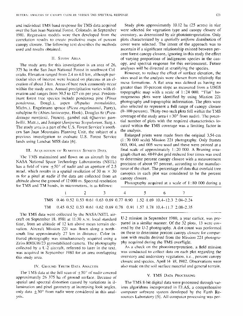
BUTERA: ANALYSIS OF CANOPY CLOSURE VERSUS TMS SPECTRAL RESPONSE l23
and individual TMS band response for TMS data acquiredover the San Juan National Forest, Colorado, in September1981. Regression models were then developed from thecorrelation results to create predictive maps of percentcanopy closure. The following text describes the methodsused and results obtained.
II. STUDY AREA
The study area for this investigation is an area of 26,375 ha in the San Juan National Forest in southwest Col-orado. Elevation ranged from 2.4 to 4.0 km, although par-ticular sites of interest were located on plateaus at an el-evation of about 3 km. Areas of bare rock commonly occurwithin the study area. Annual precipitation varies with el-evation and ranges from 30.5 to 127 cm per year. Predom-inant forest tree species include ponderosa pine (Pinusponderosa, DougL), aspen (Populus tremuloides,Michx.), Engelmann spruce (Picea engelmannii, Parry),subalpine fir (Abies lasiocarpa, Hook), Douglas fir (Pseu-dotsur;a menziesii, Franco), gambel oak (Quercus gam-bellii, Matt.), and Juniper (Juniperus Scopulorwn, Sarg.).The study area is a part of the U.S. Forest Service's south-ern San Juan Mountains Planning Unit, the subject of aprevious investigation to evaluate U.S. Forest Servicelands using Landsat MSS data [6].
III. ACQUISITIONOF REMOTELYSENSED DATA
The TMS maintained and flown on an aircraft by theNASA National Space Technology Laboratories (NSTL)has a field of view ±50° of nadir and an aperture of 2.5mrad, which results in a spatial resolution of 30 m X 30m for a pixel at nadir if the data are collected from analtitude above the ground of 12 000 m. Spectral resolutionfor TMS and TM bands, in micrometers, is as follows:
Study plots approximately 10.12 ha (25 acres) in sizewere selected for vegetation type and canopy closure ofoverstory, as determined by air photointerpretation. Onlyplots characterized by a spatially un~form distribution ofcover were selected. The intent of the approach was toascertain if a significant relationship existed between per-cent forest canopy closure, ignoring in this study the effectof varying proportions of indigenous species in the can-opy, and spectral response for this environment. Futureanalyses will be directed at stratifying the species.
However, to reduce the effect of surface elevation, thesites used in the analysis were chosen from relatively flatmesa formations. A flat area was defined as having nogreater than lO-percent slope as measured from a USGStopographic map with a scale of I:24 000. "Flat" ho-mogeneous plots were identified by using Mission 221photography and topographic information. The plots werealso selected to represent a full range of canopy closure(0-100 percent). Thirty-two such plots fell within the TMScoverage of the study area (± 30° from nadir). The poten-tial number of plots with the required characteristics lo-cated within the TMS coverage was a limiting factor inthe analysis.
Enlarged prints were made from the original 3.54-cm(1 : 70 000 scale) Mission 221 photography. Only framesom, 004, and 005 were used and these were printed at afinal scale of approximately 1 : 20 000. A Bruning area-graph chart no. 4849 dot grid reduced four times was usedto determine percent canopy closure with a measurementprecision of about 97 percent, according to the manufac-turer of the chart. The percentage of dots that overlaid treecanopies in each plot was considered to be the percentcanopy closure.
Photography acquired at a scale of I:80 000 during a
1 2 3 4 5 6 7
TMS 0.46-0.52 0.53-0.61 0.63-0.69 0.77-0.90 \.52-\.69 10.4-12.3 2.04-2.24
TM 0.45-0.52 0.53-0.61 0.62-0.69 0.78-0.91 \.57-\.78 10.4-1\.7 2.08-2.35
The TMS data were collected by the NASA/NSTL air-craft on September 18, 1981 at 11:30 A.M. local standardtime, from an altitude of 12 km above mean terrain ele-vation. Aircraft Mission 221 was flown along a north-south line approximately 27 km in distance. Color in-frared photography was simultaneously acquired using aZeiss RMK 16/23 gyrostabilized camera. The photographycollected by a U-2 aircraft, referred to later in the text,was acquired in September 1980 for an area overlappingthis study area.
IV. GROUND TRUTH DAIA ANALYSIS
The TMS data at the full scan of ± 50° of nadir coveredapproximately 26 375 ha of ground surface. Because ofspatial and spectral distortion caused by variations in il-lumination and pixel geometry at increasing look angles,only data ±30° from nadir were considered in this anal-YSIS.
U-2 mission in September 1980, a year earlier, was pre-pared in a similar manner. Of the 32 plots, 13 were cov-ered by the U-2 photography. A dot count was performedon these to determine percent canopy closure for compar-ison with results derived from the Mission 221 photogra-phy acquired during the TMS overflight.
As a check on the photointerpretation, a field missionwas conducted to collect data on each plot regarding theoverstory and understory vegetation, i.e., percent canopyclosure and species, April 14-18, 1982. Observations werealso made on the soil surface material and general terrain.
V. TMS DATA PROCESSING
The TMS 8-bit digital data were processed through var-ious algorithms incorporated in ELAS, a comprehensivecomputer software system developed by the Earth Re-sources Laboratory [5]. All computer processing was per-
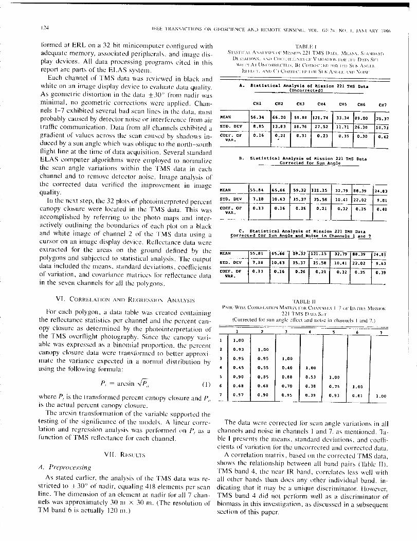
124 If'EE TRANSACTIONS ON C>f'OSCIE\lCE At.;!) REMOTE SENSI\lC>, VOL, (;10-24, NO. I, JAt\lfARY !lJX6
'[ABLE IST'\STIC.\L A\J.\IYSI'.S Cll' 'vllsslo~ 221 TMS DATA. ME,"S. SIA\JIlARIl
DLVIATIONS. '\~Il ('OU'I'ICIL~I SOl VARIATION [()K IHI· DAL\ SLI
WHI'N A) UNCORI~FCTl:Il. B) CORRI'CTLIl [()R THI'. Sr:N AN(,].r·
FITICI, ·\NIl C) CORI<I'CTLIlIOI~ SI'N A\J(']L ,\NIl Norsi'
M!:AN 55.81 65.66 59.32 121.15 32.79 88.39 24 .81STD. DEV 1.18 10.63 15.31 25.58 10.41 22.02 9.63COEf'. Of' 0.13 0.16 0.26 0.21 0.32 0.25 0.39VAR.
MEAN 56.34 66.20 59.88 121.74 J3.J4 89.00 25.37STD. DEV 8.85 13.83 lB.76 27.52 11.71 26.30 10.71COEf'. Of' 0.16 0.21 0.31 0.23 0.35 0.30 0.42VAR. ,
M!:AN 55.84 65.66 59.32 121.15 32.79 88.39 24.83STD. DEV 1.18 10.63 15.31 25.58 10.41 22.02 9.81COEf'. Of' 0.13 0.16 0.26 0.21 0.32 0.25 0.40VAR.
CH7CH6CH5CH4CR3CR2CHI
A. St.ti5tic.l An.1y.is of Mi •• ion 221 TMS Dat.(Uncorrected)
B. Statistical Analysis of Mission 221 TMS DataCorrected for Sun Angle
C. Statistical Analysis of Mission 221 TMS DataCorrected for Sun Angle and Noise in Channels 1 and 7
formed at ERL on a 32-bit minicomputer configured withadequate memory, associated peripherals. and image dis-play devices. All data processing programs cited in thisreport are parts of the ELAS system.
Each channel of TMS data was reviewed in black andwhite on an image display device to evaluate data quality.As geometric distortion in the data ±30° from nadir wasminimal, no geometric corrections were appl ied. Chan-nels 1-7 exhibited several bad scan lines in the e1ata. mostprobably caused by detector noise or interference from airtraffic communication. Data from all channels exhibited agradient of values across the scan caused by shadows in-duced by a sun angle which was oblique to the north-southflight line at the time of data acquisition. Several standardELAS computer algorithms were employed to normalizethe scan angle variations within the TMS data in eachchannel and to remove detector noise. Image analysis ofthe corrected data verified the improvement in imagequality.
In the next step, the 32 plots of photointerpreted percentcanopy closure were located in the TMS data. This wasaccomplished by referring to the photo maps and inter-actively outlining the boundaries of each plot on a blackand white image of channel 2 of the TMS data using acursor on an image display device. Reflectance data wereextracted for the areas on the ground defined by thepolygons and subjected to statistical analysis. The outputdata included the means, standard deviations, coefficientsof variation, and covariance mat rices f()r reflectance datain the seven channels fix all the polygons.
VII, RESULTS
VI. CORRELATION AND Rr'GRESSION ANALYSIS
where PI is the transformed percent canopy closure and Pois the actual percent canopy closure.
The arcsin transformation of the variable supported thetesting of the significance of the models. A linear corre-lation and regression analysis was performed on PI as afunction of TMS reflectance for each channel.
A. PreprocessingAs stated earlier, the analysis of the TMS data was re-
stricted to ±30° of nadir, equaling 418 elements per scanline. The dimension of an element at nadir for all 7 chan-nels was approximately 30 m x 30 m. (The resolution ofTM band 6 is actually 120 m.)
7652
1 1.00
2 0.93 1.00
3 0.95 0.95 1.00
4 0.45 0.55 0.40 1.00
5 0.90 0,85 0.88 0.53 1.006 0.68 0.68 0.70 0.38 0.75 1.007 0.97 0.90 0.95 0.39 0.93 0.81 1.00
TABLE 1IPAIK-WISE CORKELAlIO\J MATRIX FORCHAN\JII.S 1-7 OF EI\TIRI, MISSION
221 TMS DATA SFI
(Corrected t(lr sun angle ctrcc! and noise in channels 1 and 7,)
The data were corrected f()r scan angle variations in allchannels and noise in channels I and 7. as mentioned. Ta-ble I presents the means. standard deviations. and coeffi-cients of variation f()r the uncorrected and corrected data.
A correlation matrix. based on the corrected TMS data.shows the relationship between all band pairs (Table II).TMS band 4. the near IR band, correlates less well withall other bands than does any other individual band. in-dicating that it may be a unique discriminator. However,TMS band 4 did not perf()rm well as a discriminator ofbiomass in this investigation, as discussed in a subsequentsection of this paper.
( ] )P, = arcsin .JP;,
For each polygon, a data table was created containingthe reflectance statistics per channel and the percent can-opy closure as determined by the photointerpretation ofthe TMS overflight photography. Since the canopy vari-able was expressed as a binomial proportion, the percentcanopy closure data were transformed to better approxi-mate the variance expected in a normal distribution byusing the following formula:
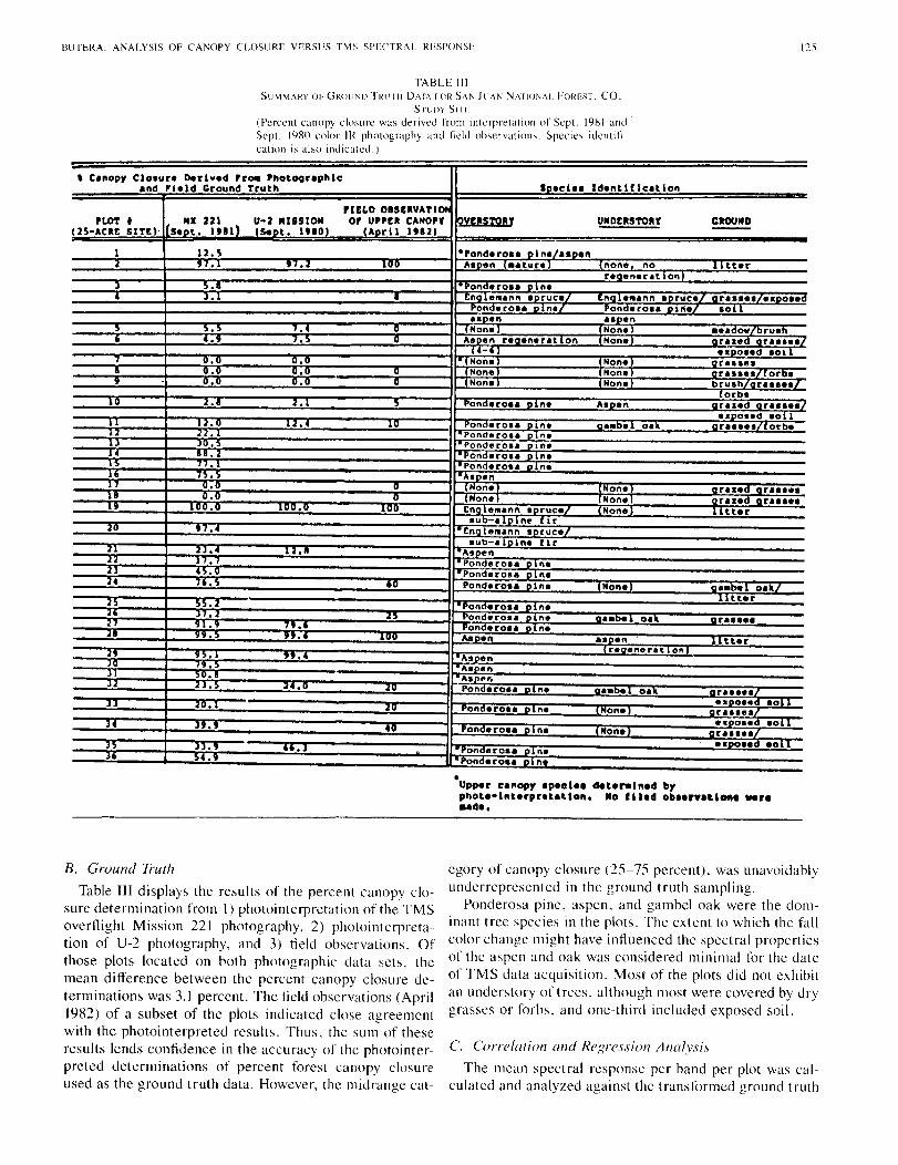
BUTERA: ANALYSIS or CANOPY CLOSURE VERSUS TMS SPECTRAL RESPONSE
TABLE IIISUMMARY 01' GROLND TRUTH D,\TA FOR SAN JUAN "lArloNAL FOREST. CO.
STUDY SI II:
(Percent canopy closure was derived from interpretation of Sept. 1981 andSept. 1980 color IR photography and field ohservations. Species identifi,cation is also indicated.)
125
, C.nopy Clo.ur. Deriv.d rr~ 'hotoor.phie.nd rl.ld Ground Truth S".el •• Id.ntiflutlon
rlELD DISUVATIOfo'LOT • fl. 221 t) U-2 IlIlUOM or U"EIl CANOPY UIlDUSTORr CllOUlfD
12S-ACRE SITE)' S."t. 1911 ISe"t. ItlOI IADrl1 Itl21 ---I 12,S ·Pond.ro •• Dln.I •• D.n2 97, ~.T JUU A.oen •• ture none, no Utt.r
r."an.~.tlonJ !I,ll ·Pond.~o•• Din.4 ],1 • EnOle".nn .D~uc.1 Eno I••••nn ."rue.7·"-r ••••• '•• Do •• a
Pond.~o •• Din. Ponaaco •• "'In.' .011•• D.n •• o.n!I !I,!I ,. 0 INone INon.l .e.dov/b~u.h" 4.9 ,!I U A.Den r.a.n.r.t on INon.I' nr.l.a "~.e•••1
14-6 •• Do •• d .01O,u 0,0 'INon. INona n~.ssesII 0,0 ,n 0 INona INon. -n-~••• e. oro.9 0,0 0.0 U INon. INon. b~u.h/or•••••1
10 1,1 T~T'orb.
!I Pond.co•• Din. A.o.n nr.z.d or ••••• '1 ,~'
•• Do •• d .0 1JU Ponde~o•• Ine o •• b. o.k n~•••••'Eorb.
Pondero •• nePondero •• ,n.·ponde~o•• ne, Pond. ~o•• n.· Aaoen
U (Non •• INon. "r.l.a or •••••U (Nonel INon. o~.z.d or •••••IC 1II1r", 0· 100 Enole •••nn .D~uc.1 INon. n.r
20 97,4 .ub-.lolne If!:nale•••nn .o~uc.'
.ub-.lDln. U~· r,II As~nPonde~o•• Din.Ponde~oa. Dineau Pond.ro •• Din. INon. n •• bel o.kl
, tt.r'Pond.ro •• 0 n.'II."
Pond.~o•• Dine "•• b.1 o.li" "r •••••· Pondero •• Din., .11,-. JUU AIIoen •• ".n tt.r211 9' , -~-;.- lrede"oret onllO 19,!I A"Dan]I !lD,1 A.D.n
A.D""1: ,~ 2 •• 0 2U Pond.ro •• "'In. a•• b. 0." n~•••••10. 2U ponll.~o•• "In. •• DO•• •0LlINon. nr •••••
It n,. • JlOO •• .0.1• U pond.ro •• "In • INon. "r •••••I!I JJ,II 46.] •• DO •• .0 1I" ~·.9 ·Ponda~o•• Din.
I·Ponll.~o•• Din.eUpper e.nopy .peele. doto~lnod by
photo-lntorpr.t.tion. Mo Illod Db.or •• tlOft. wore•• do,
B. Ground Truth
Table III displays the results of the percent canopy clo-sure determination from 1) photointerpretation of the TMSoverflight Mission 221 photography, 2) photointerpreta-tion of U-2 photography, and 3) field observations. Ofthose plots located on both photographic data sets, themean difference between the percent canopy closure de-terminations was 3.1 percent. The field observations (April1982) of a subset of the plots indicated close agreementwith the photointerpreted results. Thus. the sum of theseresults lends confidence in the accuracy of the photointer-preted determinations of percent forest canopy closureused as the ground truth data. However, the midrange cat-
egory of canopy closure (25-75 percent). was unavoidablyunderrepresented in the ground truth sampling .•
Ponderosa pine, aspen. and gambel oak were the dom-inant tree species in the plots. The extent to which the fallcolor change might have influenced the spectral propertiesof the aspen and oak was considered minimal for the dateof TMS data acquisition. Most of the plots did not exhibitan understory or trees, although most were covered by drygrasses or forbs, and one-third included exposed soil.
C. Correlation and Regression AnalysisThe mean spectral response per band per plot was cal-
culated and analyzed against the transformed ground truth
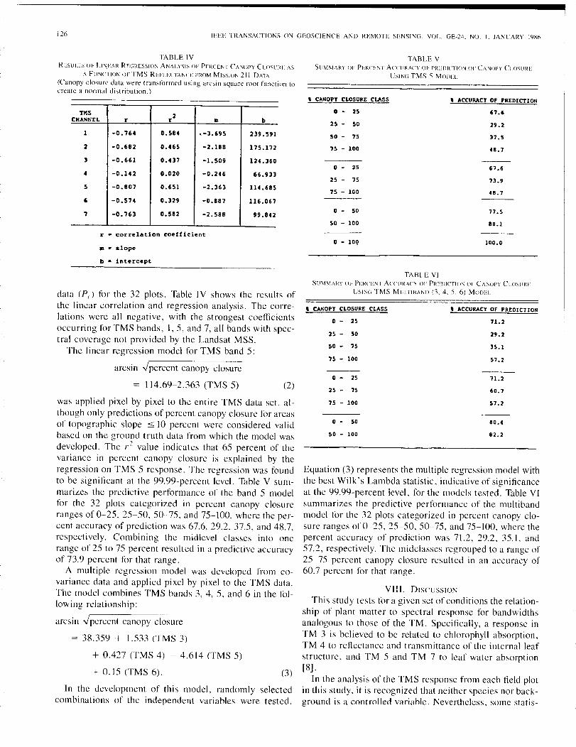
126 IEEE TRANSACTlOT\S ON GEOSCIENCE AND REMOTE SENSING, VOL. GE-24, NO. L JAT\lJARY 1986
TABLE VSUMMARY OF PERCEI\T ACCURACY OF PREDICTION 01' CANOPY CLOSURE
USIN« TMS 5 MODEL
TABLE IVRESUlT:> Or LIN,EAR Rr:«RESSIOI\ ANALYSIS OF PERCENT CANOPY CLOSLRE AS
A FUNCTION OF TMS REFLFCTANCF FROM MISSION 211 DATA
(Canopy closurc data were transformcd using arcsin square rool function tocreatc a normal distribution.)
, CANOPy CLOSURE CLASS , ACCURACY OF PREDICTION
TPIS 2CHANNEL r r •• b
I -0.764 0.584 • -3.695 239.591
2 -0.682 0.465 -2.188 175.172
3 -0.661 0.437 -1.509 124.360
4 -0.142 0.020 -0.246 66.933
5 -0.807 0.651 -2.363 1l4.U5
6 -0.574 0.329 -0.887 116.067
7 -0.763 0.582 -2.588 99.842
o - 25
25 - so50 - 75
75 - 100
o - 25
25 - 75
75 - 100
o - SO
50 - 100
67.6
29.2
37.5
48.7
67.6
73.9
48.7
77.5
88.1
r • correlation coefficient••• slope
o - 100 100.0
b • intercept
In the development of this model, randomly selectedcombinations of the independent variables were tested.
data (PI) for the 32 plots. Table IV shows the results ofthe linear correlation and regression analysis. The corre-lations were all negative, with the strongest coefficientsoccurring for TMS bands, 1,5, and 7, all bands with spec-tral coverage not provided by the Landsat MSS.
The linear regression model for TMS band 5:
arcsin ,Jpercent canopy closure
was applied pixel by pixel to the entire TMS data set, al-though only predictions of percent canopy closure for areasof topographic slope ~ 10 percent were considered validbased on the ground truth data from which the model wasdeveloped. The ,.2 value indicates that 65 percent of thevariance in percent canopy closure is explained by theregression on TMS 5 response. The regression was foundto be significant at the 99.99-percent level. Table V sum-marizes the predictive performance of the band 5 modelfor the 32 plots categorized in percent canopy closureranges of 0-25, 25-50, 50-75, and 75-100, where the per-cent accuracy of prediction was 67.6, 29.2, 37.5, and 48.7,respectively. Combining the midlevel classes into onerange of 25 to 75 percent resulted in a predictive accuracyof 73.9 percent for that range.
A multiple regression model was developed from co-variance data and applied pixel by pixel to the TMS data.The model combines TMS bands 3, 4, 5, and 6 in the fol-lowing relationship:
arcsin ,Jpercent canopy closure
TABLE VISUM\1ARY OF PERCEN r ACCURACY 01· PREDICTIOI\ OF CANOPY CLOSURE
USII\(; TMS MLLTIBAI\IJ (3. 4. 5. 6) MODEL
71.2
29.2
35.157.2
71.2
57.2
60.7
80.4
82.2
, ACCURACY Of PREDICTION
o - 50
so - 100
o - 25
25 - 75
75 - 100
o - 25·25 - SO
50 - 75
75 - 100
, CANOPY C~OSURE CLASS
Equation (3) represents the multiple regression model withthe best Wilk's Lambda statistic, indicative of significanceat the 99.99-percent level, for the models tested. Table VIsummarizes the predictive performance of the multibandmodel for the 32 plots categorized in percent canopy clo-sure ranges of 0-25, 25-50, 50-75, and 75-100, where thepercent accuracy of prediction was 71.2, 29.2, 35. I, and57.2, respectively. The midclasses regrouped to a range of25-75 percent canopy closure resulted in an accuracy of60.7 percent for that range.
VIII. DISCUSSION
This study tests for a given set of conditions the relation-ship of plant matter to spectral response for bandwidthsanalogous to those of the TM. Specifically, a response inTM 3 is believed to be related to chlorophyll absorption,TM 4 to reflectance and transmittance of the internal leafstructure, and TM 5 and TM 7 to leaf water absorption[8] .
In the analysis of the TMS response from each field plotin this study, it is recognized that neither species nor back-ground is a controlled variable. Nevertheless, some statis-
(2)
(3)
= 114.69-2.363 (TMS 5)
38.359 + 1.533 (TMS 3)
+ 0.427 (TMS 4) - 4.614 (TMS 5)
+ 0.15 (TMS 6).

BUTERA: ANALYSIS OF CANOPY CLOSURE VERSUS TMS SPECTRAL RESPONSE ]27
1
•••• -0.52 0.53-0.&1 D.U-4I." D.77-D.tD 1.52-1.U ID.<-n.l. 2.Dt-2.2<
Fig. I. Generalized spectral response curves for vegetation and soil (after[9, Figs. 5-10 and 5-13]). These curves provide an understanding con-ditions of high spectral contrast that can occur between background andtarget.
tically significant results occurred that can be supportedby reasonable biophysical explanations.
An analysis of the correlation results for percent canopyclosure versus TMS spectral response must address theintegrated effect of target and background on reflectance.In this investigation, the correlation between canopy clo-sure and spectral response was negative for all bands, in-dicating that the mean response decreased as canopy clo-sure increased. If one considers the background of driedgrasses or exposed soil, it may be hypothesized that theseelements contributed relatively higher reflectance valuesthan did the forest canopy to the overall scene. Plots witha greater percentage of canopy closure, then, also had alesser percentage of the more highly reflective groundcover contributing to the spectral signature. Indeed, pub-lished spectral reflectance curves for vegetation and soilsupport this idea (Fig. I). In the figure, reflectance curvesfor low-moisture-content vegetation and dry sand are bothhigher than for turgid vegetation.
The absolute correlation coefficient was higher for therelationship between TMS 5 and the transformed percentcanopy closure than for any other band. Again referringto general reflectance curves for vegetation and soil in Fig.I, one may infer that for the interval 1.52 to 1.69 /-Lmcor-responding to TMS band 5, it is possible that the distancebetween curves of turgid vegetation and a background ofsoil and senescing grasses might be maximized. No datawere acquired representing the individual tree canopy andbackground spectral contributions to substantiate this hy-pothesis, however.
The low correlation between canopy closure and TMSband 4 was surprising in that this band is assumed to relateto internal leaf structure, which implies a relationship tobiomass, at least in the case of herbaceous material. Fig.2 displays relative signal response curves for three groundtruth plots with O-percent canopy closure and three groundtruth plots with nearly 100-percent canopy closure, dem-onstrating the lack of discrimination in TMS band 4 withrespect to the true canopy variable. It is possible that for
the particular conditions of the forest target and back-ground soil and grasses in this study, reflective responsesmeasured for the spectral coverage represented by TMSband 4 may have been relatively equal. Fig. 2 clearly dem-onstrates the greater separability between curves of 0- and100-percent canopy closure for TMS bands 1, 5, and 7.
Regression models to predict canopy closure from spec-tral response were developed from the results of this studyand applied to each pixel to gain an understanding of theperformance of the models and manipulations that couldbe executed on the imagery.
In development of the regression models to predict can-opy closure, the influence of topographic slope as a vari-able was intentionally minimized. Vegetation species as avariable was minimized to some extent, but not elimi-nated, as the area considered for the analysis was domi-nated by ponderosa pine and aspen with lesser coverageby Douglas fir, Engelmann spruce, and gambel oak. Thus,it can be said that valid application ofthe models to predictpercent canopy closure for this environment allows for as-sociations of species and is not restricted to a monospe-cific condition.
A recommendation for the most accurate technique forprediction of percent canopy closure based on the resultsof this investigation can be derived by examination of theprediction accuracies summarized in Tables V and VI. Itis apparent that these accuracies are lower for the middleclasses of canopy closure, i.e., 25-50 and 50-75 percent.Dottavio [3] also noted greater difficulty in estimatingcanopy closure for the midranges using her incoming solarradiance technique. Regrouping the middle classes intoone range class of 25-75 percent raises the accuracy, al-though the utility of such a broad class may be questioned.
Using only the techniques evaluated in this investiga-tion, a combination of the results from the application ofthe single-band and multiband models is recommended.The optimum overlaying of the two data sets would in-clude pixels with estimates from the band 5 model only forthe 25-75 percent canopy closure class and pixels withestimates from the multiband model for the 0-25 and 75-100 percent classes. By combining results of the twomodels predictive accuracies for canopy closure classes of0-25, 25-75, and 75-100 percent would then be 71.2, 73.9,57.2 percent, respectively.
This investigation focused on correlation analysis andregression model development to predict percent canopyclosure from TMS spectral response. A follow-on effortshould include an evaluation of other techniques, such asfeature extraction, canonical correlation, and brightness!greenness component analyses. It should also include con-trol of obvious variables such as number of species, theirdistribution within a plot, and the background material.As well, the performance of the models should be evalu-ated on an independent data set.
IX. CONCLUSIONS
Based on the results of this study, the following conclu-sions were reached:

128
160
140
120
100•...!=!<-~•..'-' eo'"•...>~<:;::'"
60
40
20
o
IEEE TRAKSACTIONS ON GEOSCIENCE AND RRMOTE SENSING, VOL. GR-24, KO. I, JANUARY 1986
0\ Crown Cover--------97-100\ Crown Cover
: : l.
·.· .· .·.· .·.·.· ., .·.· ,
..'. :
":,:ii;..:,.
.:.":"f:
!!!f
,. ff... " •..~ _.- ii~.--- ..•.•..•.•.;i.......,J
3 5 6
TIIS CHANNELFig. 2. Graph of relative reflectance versus TMS channels I()r Mission 221
data. Graphs demonstrate discrimination capahility of TMS 5 for canopyclosure, (CO test site, Sept. 18, 1981.)
TMS bands 1,5, and 7, essentially wavelength intervalsnot covered by the Landsat MSS, proved most significantin relating percent forest canopy closure to spectral re-sponse.
The negative correlations resulting from the analysis ofpercent canopy closure and TMS spectral response for allbands were probably caused by a spectral contributionfrom the background (dry soil, senescing grasses) withhigher reflectivity than that of the forest canopy.
The results of this investigation were specific to eco-system type, time of year, and absence of slope.
For a given ecosystem, the best predictive model is de-veloped when conditions of greatest spectral contrast be-tween background and forest vegetation occur.
The techniques developed and conclusions reached inthis TMS study are applicable to the utilization of TM data.
ACKNOWLEDGMENT
Special thanks are extended to M. Kalcic for her assis-tance in the statistical analysis in this investigation and toDr. A. Joyce and J. Ivey for providing direction and co-ordination of activities related to this study.
REFERENCES
II] J. E. Anderson and M. T. Kalcic, "Analysis of thematic mapper sim-ulator data acquired during the winter season over pearl river. MS TestSite." AgRISTARS Tech. Rep. RR-YI-04217. '-JSTLlERL-202. Na-tional Technical [nl(lrI11ation Service. Springfield. VA. 1982.
121 L. E. Blanchard and O. Weinstein. "Design challenges of the the-matic mapper." IEEE Truns. Geosci. ReJilole Sensing. vol. GE-18, no.2, pp. 146-160. 1980.
13] C. L. Dottavio. "EIl'cct of forcst canopy closure on incoming solarradiance." in Proe. /981 Machine Processing o{Re/llOlely Sensed DalllSI'/Ilp. (Purdue Univ .. West Lafayette. IN). pp. 375-383, 1981.
141 C. L. Dottavio and D. L. Williams. "Mapping a southern pine planetat ion with satellite and aircraft scanner data: A comparison of presentand future landsat sensors." 1. Appl. Pho!o. /:·ng., vo!. 8, no. I. pp.58-62. 1982
15] B. G. Junkin, el al., "ELAS-Earth resources laboratory applicationssoftware rep. 183." NASA/NSTL Resources Lab., NSTL Station, MS.1981.
16] P. V. Krebs, 1'1 al., "Multiple resource evaluation of region 2 U.S. For-est Service lands utilizing Landsat MSS data." Type [[]-Final Rep.NA55-20948. National Technical Inl()fmation Service. Springfield. VA,1976.
171 V. V. Salomon son , el al., "An overview of progress in the design andimplementation of Landsat-!) systems." IEEE 7h/fls. Geosci. RemoleSensing, vol, GE-18, no, 2. pp. \37-146. 1980.
18J P. H. Swain and S. M. Davis, Eds. Remole Sensing: The Quallli!ativeApproach. :'-Jew York: McGraw-Hili. 1978, p. 386.
19] C. J. Tucker, "A comparison of satellite sensor bands for vegetationmonitoring." Pho!ogrummetr. Eng .. vol. 44, no. II, pp. \369-1380,1978.

BUTERA: ANALYSIS OF CANOPY CLOSURE VERSUS TMS SPECTRAL RESPONSE 129
M. Kristine Butera (M'84) received the B.A. andM.A. degrees in plant physiology from the Uni-versity of Missouri at Columbia in 1969 and 1970,respectively.
She is Deputy Program Manager at ScienceApplications International Corporation in Wash-ington, DC, engaged in contract rescarch forNASA Headquarters. She was principally respon-sible for the drafting of the revision of the agency-level basic agreement between NASA and NOAAon space-related programs and is currently leading
a task to evaluate the status of access and capability for distributed data
systems supporting NASA-sponsored Earth Science research. Formerly, shewas an employee and principal investigator of NASA from 1974 to 1984 andconducted research and appl ications in remote sensing of coastal and for-ested areas from aircraft and satellite platforms. During her employmentwith NASA, she served as Headquarters Program Manager for fundamentalremote-sensing science in the Land Processes Branch of the Office of SpaceScience and Applications and was involved with the selection of proposalsrelated to the Thematic Mapper Announcement of Opportunity. She alsoworked at NASA/GSFC in the planning of the Pilot Land Data System andat NASA/NSTL where she conducted AgRISTARS-related studies andcoastal remote-sensing investigations. She is a technical reviewer for tworemote sensing journals and has published numerous invited papers.
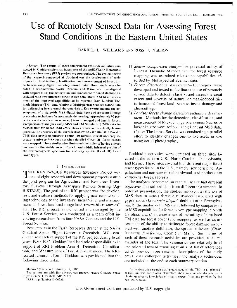
130 JEEE TRANSACTIONS ON GEOSCIENCE AND REMOTE SENSING, VOL. GE-24, NO. I. JANUARY 19X6
Use of Remotely Sensed Data for Assessing ForestStand Conditions in the Eastern United States
DARREL L. WILLIAMS AND ROSS F. NELSON
Abstract- The results of three interrelated research activities con-ducted by Goddard scientists in support of the AgRISTARS RenewableResources Inventory (RRI) project are summarized. The central themeof the research conducted at Goddard was the development of tech-niques for the detection, classification, and measurement of forest dis-turbances using digital, remotely sensed data. Three study areas lo-cated in Pennsylvania, North Carolina. and Maine were investigatedwith respect to: a) the delineation and assessment of forest damage as-sociated with two different forest insect def()liators, and b) an assess-ment of the improved capabilities to be expected from Landsat The-matic Mapper (TM) data relative to Multispectral Scanner (MSS) datafor delineating forest stand characteristics. Key results include the de-velopment of a statewide MSS digital data base and associated imageprocessing techniques for accurately delineating (approximately 90 per-cent correct classification atturacy) insect damaged and healthy forest.Comparison of analyses using MSS and TM Simulator (TMS) data in-dicated that for broad land cover classes which are spectrally homo-geneous. the accuracy of the classification results are similar. However,TMS data provided superior results (20 percent overall atturaty in-crease relative to MSS results) when detailed (Level III) forest classeswere mapped. These studies also illustrated the utility of having at leastone band in the visible. near infrared. and middle infrared portion ofthe electromagnetic spectrum for assessing specific (Level III) foresttover types.
I. INTRODUCTION
THE RENEWABLE Resources Inventory Project wasone of eight research and development projects within
the joint program for Agricultural and Resources Inven-tory Surveys Through Aerospace Remote Sensing (Ag-RISTARS). The goal of the RRI project was "to develop.test, and evaluate methods for applying new remote sens-ing technology to the inventory. monitoring, and manage-ment of forest land and range land renewable resources"r I]. The RRI project, implemented and managed by theU.S. Forest Service, was conducted as a team effort in-volving researchers from four NASA Centers and the U.S.Forest Service.
Researchers in the Earth Resources Branch at the NASAGoddard Space Flight Center in Greenbelt. MD, con-ducted research in support of the RRI project during fiscalyears 1980-1982. Goddard had lead role responsibilities insupport of RRI Problem Area 4-Detection. Classifica-tion. and Measurement of Forest Disturbances. The RRI-related research effort at Goddard was partitioned into thefollowing three tasks.
Manuscript received February 15, 1985.The authors arc with Earth Resources Branch, NASA Goddard Space
Flight Center, Greenbelt, MD 20771.IEEE Log Number 8406228.
I) Sensor comparison study-The potential utility ofLandsat Thematic Mapper data for forest resourcemapping was examined relative to capabilities af-forded by Multispectral Scanner data. I
2) Forest disturbance assessment-Techniques weredeveloped and tested to facilitate the use of remotelysensed data to detect, classify. and assess the arealextent and severity of natural or man-induced dis-turbances of forest land, such as insect damage andclearcutting.
3) Landsat forest change detection technique develop-ment-Methods for the detection. classification. andmeasurement of forest change phenomena 5 acres orlarger in size were refined using Landsat MSS data.(Note: The Forest Service was conducting a paralleleffort to identify changes one to five acres in sizeusing aerial photography.)
Goddard's actIvItIes were centered on three sites lo-cated in the eastern U.S.: North Carolina. Pennsylvania.and Maine. These sites covered four different major forestcover types found in the U.S,, namely. southern pine. Ap-palachian and northern mixed hardwood, and northeasternspruce-fir (boreal) forests.
The analyses conducted on each study site had differentobjectives and utilized data from different instruments. Inorder of presentation. the studies involved: a) the use ofMSS data to assess forest disturbances associated withgypsy moth (Lymantria dispar) defoliation in Pennsylva-nia. b) the analysis of TMS data, followed by comparisonsto MSS capabilities for forest cover type mapping in NorthCarolina. and c) an assessment of the utility of simulatedTM data for forest cover type mapping, as well as an as-sessment of the ability to delineate forest damage associ-ated with another defoliator. the spruce budworm (Chor-istoneura fumiferana. Clem.) in Maine. Summaries ofeach of these research activities are provided in the re-mainder of the text. The summaries are relatively briefand oriented toward reporting results. A list of referenceswhich provide more detailed descriptions of the studyareas, data collection activities. and analysis techniquesare included at the end of each summary section.
'At the time this research was being conducted, the TM was a "planned"sensor, and was not in orbit. Therefore. there was considerable interest inobtaining advance knowlcdgc of what to cxpcct from data provided by thisnew instrumcnt.
U.S. Government work not protected by U.S. copyright

WILLIAMS AND NELSON: REMOTELY SENSED DATA FOR ASSESSING FOREST STAND CONDITIONS 131
II. AN MSS DIGITAL DATA BASE TO DETECT FORESTDISTURBANCE(PENNSYLVANIA)
A. BackgroundIn the mid to late 1970's, procedures were developed at
Goddard which proved useful for delineating gypsy mothdefoliation damage over relatively small areas (i .e., lessthan one Landsat scene) using Landsat MSS data. Theseprocedures involved: a) the use of multitemporal. L~ndsatdata acquired "before" and "after" peak defoltatlOn tofacilitate the detection of change associated with the defo-liation, b) the use of a simple band ratioing technique toassess the severity of defoliation, and c) the use of a dig-itally derived forestlnonforest mask to eliminate errors ofcommission with non forest cover types when applying for-est change detection techniques. The applicability of theseprocedures to large areas encompassing the equivalent ofseveral Landsat scenes needed to be tested. Under RRI,these procedures were integrated to form an automatedsystem for making annual assessments of the areal extentand severity of gypsy moth defoliation for the entire stateof Pennsylvania using Landsat MSS data.
B. Data Base CharacteristicsThe assessment of insect defoliation damage over an
area as extensive as Pennsylvania using Landsat MSS datarequired the processing and storage of tremendous quan-tities of data. The state is covered by portions of 10 Land-sat scenes, with each scene containing approximately 7.5million picture elements (pixels). Therefore, a systemwhich could accommodate efficient digital processing aswell as storage and retrieval of these data had to be de-veloped.
A data base was created which incorporated Landsatdata, thematic information, and digital data products. Thedata base was registered to the Universal Transverse Mer-cator (UTM) map projection and output in a grid formatconsisting of 57-m2 cells.2 The data base, which resideson an IBM 370/3081 computer at the Pennsylvania StateUniversity Computation Center, includes a number of"layers" of thematic information as depicted in Fig. 1.
C. Analysis ProceduresPersonnel of the Office for Remote Sensing of Earth Re-
sources (ORSER) at the Pennsylvania State University de-veloped a series of computer programs to facilitate thestorage, retrieval, and analysis of data within the database. With these programs, the user can step through aseries of procedures to produce a defoliation assessmentimage over any portion of the state. The steps involved ina typical analysis scenerio follows.
I) Acquire the most recent MSS data and register it tothe data base. This step requires a remote-sensinganalyst familiar with image processing software.Steps 2 through 6, however, may be performed bynonremote-sensing personnel.
2Fifty-seven meters is the nominal pixel size of processed MSS data. Theinstantaneous field-of-view of the MSS is approximately 80 nl.
UTM ZONE 18
Data
1.3'ldsal Data Depicting DefoliationConditions
Fig. I. Characteristics of the Pennsylvania Statewide Digital Data Basc.
2) Select the area of interest. County and forest districtboundaries are available in the data base. In addi-tion, the user may specify any arbitrary subsectionof the state.
3) Apply the forestlnonforest mask. Previous work atGoddard had shown that some agricultural areas arespectrally similar to defoliated forests. To overcomethe associated errors of commission, nonforest areasare digitally masked and dropped from considera-tion. The forestlnonforest mask is an integral part ofthe digital data base and was developed from Land-sat data depicting healthy forest conditions in Penn-sylvania between 1976 and 1979. This mask wouldhave to be updated periodically to reflect changesdue to forest harvesting activities, regrowth, etc.
4) Calculate the MSS Band 7/Band 5 ratio. This ratio,comprising thenear infrared spectral response in thenumerator and the red response in the denominator,has been shown to be proportional to the amount ofgreen biomass in the sensor field-of-view [23]. Asthe amount of green vegetation increases, the 7/5ratio increases. Defoliated forests thus have low ra-tios relative to healthy forest.
5) Classify the 715 ratio image into defoliated and non-defoliated forest stands. This step entails imagethresholding. Work done during this project estab-lished an approximate threshold for distinguishingbetween healthy forest and heavily defoliated forest.Subsequent work has shown that this threshold canvary between Landsat scenes and between years.Hence, a number of classification trials may be nec-essary to produce an acceptable classification.
6) Produce appropriate output products such as tabularstatistics, classification images, or line printer maps.
D. ResultsThe utility of Landsat MSS data for assessing forest dis-
turbances depends on the success of a preprocessing step-the delineation of forest and nonforest. Studies at Goddardhave shown that MSS data can be used to reliably distin-guish forested areas from nonforested areas using growingseason data. Classification accuracies consistently fallwithin the 85-95 percent range. The accuracy of the for-est/nonforest mask for the entire state of Pennsylvania was

132 IEEE TRANSACTIONS ON GEOSCIENCE AND REMOTE SENSING. VOL GE-24. NO. L JANUARY In6
'1II
I
I
III
l'I
II
I
\
\
"", ,,
HEN ..THY FORESTMODERATE DEFOLIATION -------
H,AVY DEFDLIATION
TABLE IC()MI'AHIS()N ()I' TM/TMS' AND MSS SE~S()H CHARACTERISTICS
1M/1MS MS;?SI'ECTHAL I:lAND ] 0.45 O,5L Jlfil O.!') o. ti .umSPECTRAL RAND 2 0.52 0.60 )lID 0.6 0.7 ~SPECTRAL HAND ] 0.6] O.b9 )lID 0.7 O.H pmSPECTI~A1 BANl1 4 0.76 0.90 ;un O. B 1.1 pmSPECTRAL HAND " 1.55 1.75 )..lID
SPECTRAL HAND 7 ~. DH 2.:;5 pmSPECTRAL BANll 6 !D.40 12.50 pmHF'OV :JGM ( HANDS 1 -5,7)' H2M
120M (HANIl (ljQUANTIZATION Lft~Vft:LS 256 64
tj~nti~~l. pr¥h~i~~be~i~~o~~~~etlfi1on£m~:st';r~er~avi~a~~n~i~f~~~ru~i~hst~~iused for the 1M (see footnot •. 4) .
• ~~~u~~Yrio~P~lfn~~~i~g~v~i~~~dgr'~~~d J~~er~i~e~het.~. sP~~ior~e~~f~{i~g~In thHI paper, all 1MS data were resampled to 30 meter rells.
BAND 7;BAND 5 RATIO
Fig. 2. The near infrared/red (band 7/hand )) ratio response of heallhyj(,rest. Illoderate def(,liation, and heavy def(lliation.
90 percent. A concise review of the production and as-sessment of the statewide forest/nonf()rest mask for Penn-sylvania is provided by Russo and Stauffer 121I.
The use of Landsat MSS data !()r delineating gypsy mothdefoliation is limited by the spectral characteristics of dif-ferent ]evels of canopy damage. MSS data may be used todifferentiate heavy def()]iation (60-]00 percent of the can-opy removed) from healthy vegetation. Attempts to dif-ferentiate three forest classes-heavy defoliation, moder-ate def()l iation (30-60-percent canopy removed), andhealthy f()rest (0--30-percent canopy removed)-h:1Veshown that moderate defoliation and healthy forest arespectrally inseparable (Fig. 2). Hence, only relativelygross canopy differences can be distinguished using Land-sat MSS data. MSS def()liation classification results agreedwith photo-interpreted results 77 percent of the time whentwo forest classes were considered (i.e., def()liated andhealthy). It should be noted that the MSS-derived c]assi-fication results were much more detailed at the ]ocal levelthan were the photointerpreted results. With MSS data, adecision is made on a pixel-by-pixel basis, where each pixelrepresents approximately three to f(mr tenths of a hectarc.On the other hand, a photointerpreter tends to assess gen-eral conditions over areas within the photo which maycomprise severa] hectares.
The use of MSS data is somcwhat limited by the tem-poral frequency of coverage (16 days), because the tem-poral window within which dcfo]iation occurs at detcct-ablc levels is re]ativcly short. Studies by Nelson [16] in-dicated that there was, at best, a two-month window fromlate June to mid-August for assessing gypsy moth defol-iation damage. Given the 16-day rcpeat cycle of the cur-rent Landsat 4 and 5 satellites, one has at best three tofour chances to acquire useful (i.e .. relatively cloud-free)data over any given portion of the state during the windowdefined by Nelson.' Since the eastern states arc often ob-scured by clouds morc than 50 percent of the time duringthe summer months 16], a real problcm exists in that one
'Actually the numher of chances is increased by a factor of two whentwo satellites are in phased orhit at the same lime. which is currently thecase for MSS data acquisition by Landsat's 4 and 5.
cannot count on MSS data as the only sourcc of informa-tion for assessment purposes. Thus, the potcntial for sig-nificant cost savings is negated by the need to have a fall-back source of data (i.e., to be safe, one must continuethe currently used approach of aerial sketch mapping and/or acquisition of aerial photography).
For more information relative to the devclopment of thePennsylvania data base and the data analysis software, thefollowing may be consulted: [5], 16[. [241. [2XI. 130].Works by Nelson [16], []8], [19] provide in-depth discus-sions of forest change detection using Landsat data andthe temporal aspects of gypsy moth damage assessment.
Ill. MSS AND SIMULATEDTM DArA FOR FORESTCOVER TYPE MAPPING (NORTH CAROLINA)
A. BackgroundTwo airborne multispectral scanners capablc of collect-
ing data with spectral, spatial, and radiometric propertiessimilar to those of the TM (Table I) were developed andflown by NASA Centers to providc simulated TM data toresearchers prior to the launch of Landsat -D 4 The ratio-nale for these data collection/analysis eft()rts was: a) to al-low researchers to bccome fami] iar with the improvedspatial. spectral, and radiometric characteristics of TMdata; b) to permit advancc developmcnt of new softwareto takc better advantage of the information contained inthis data; and c) to quantify the improvements to be ex-pected from TM data relative to MSS data for specific ap-pI ications [261.
An investigation was undertaken to examine the utilityof TM data for Jorest resource mapping. Thc study wasdivided into two segments. The first segment involved acomparison of simulated TM and actual MSS data to de-termine which sensor was more suitable for forest re-sources inventory and assessment. The second segmcntwas directed toward developing methods of reducing thelarge volume of data inhercnt to the 'I'M sensor by deter-mining the optimum subset of spectral bands for identi-fying forest cover types.
"For all practical purposes. the speelral hands provided hy the TM sim-ulator devices were identical to those provided hy the TM. However. I(lrhoth TMS devices. the numberin~ of the hands ditrcred sliuhtlv from theTM due to the inclusion or additional hands. elc. 'Ii, redue~ c,;nrusion inthis paper. all TMS hands will bc identified hy their TM equivalenl handnumher.
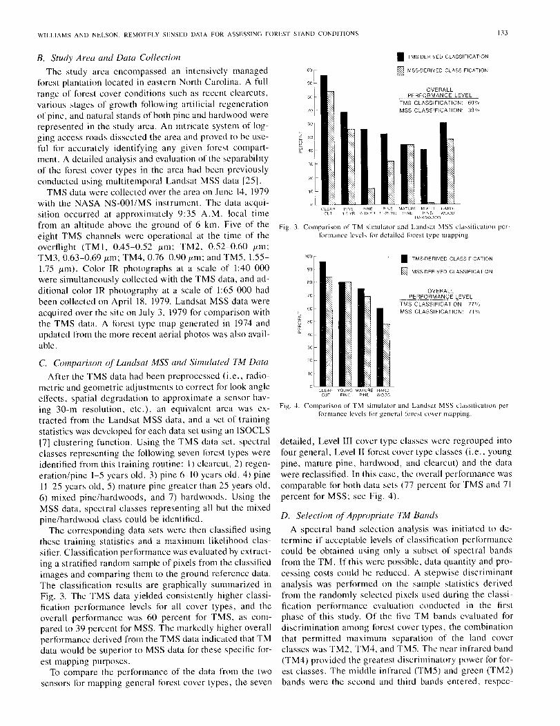
WILLIAMS AND NELSON: REMOTELY SENSED DATA FOR ASSESSING FOREST STAND COJ\DITIONS 133
Fig. 4. Comparison of TM simulator and Landsat MSS classilication per-f{)fmUnCe levels for general forest cover mapping.
Fig. 3. Comparison of TM simulator and Landsat MSS classification per-j(lfInance levels for detailed !()resl type mapping.
OVERALLPERFORMANCE LEVEL
TMS CLASSIFICATION: 60%MSS CLASSIFICATION: 39%
• TMS·DERIVED CLASSIFICATION
~ MSS·DERIVED CLASSIFICATION
OVERALLPERFORMANCE LEVEL
TMS CLASSIFICATION: 77%MSS CLASSIFICATION: 71 %
70
30
10
20 -
60
eo
100
f-Z
~ 50IE0.
• TMS·DERIVED CLASSIFICATION
~ MSS·DERIVED CLASSIFICATION
D. Selection of Appropriate TM BandsA spectral band selection analysis was initiated to de-
termine if acceptable levels of classification performancecould be obtained using only a subset of spectral bandsfrom the TM. If this were possible, data quantity and pro-cessing costs could be reduced. A stepwise discriminantanalysis was performed on the sample statistics derivedfrom the randomly selected pixels used during the classi-fication performance evaluation conducted in the firstphase of this study. Of the five TM bands evaluated fordiscrimination among forest cover types, the combinationthat permitted maximum separation of the land coverclasses was TM2, TM4, and TM5. The near infrared band(TM4) provided the greatest discriminatory power for for-est classes. The middle infrared (TM5) and green (TM2)bands were the second and third bands entered, respec-
detailed, Level III cover type classes were regrouped intofour general, Level II forest cover type classes (i.e., youngpine, mature pine, hardwood, and clearcut) and the datawere reclassified. In this case, the overall performance wascomparable for both data sets (77 percent for TMS and 71percent for MSS; see Fig. 4).
C. Comparison of Landsat MSS and Simulated TM DataAfter the TMS data had been preprocessed (i.e., radio-
metric and geometric adjustments to correct for look angleeffects, spatial degradation to approximate a sensor hav-ing 30-m resolution, etc.), an equivalent area was ex-tracted from the Landsat MSS data, and a set of trainingstatistics was developed for each data set using an ISOCLS[7] clustering function. Using the TMS data set, spectralclasses representing the following seven forest types wereidentified from this training routine: I) clearcut, 2) regen-eration/pine 1-5 years old, 3) pine 6-10 years old, 4) pine11-25 years old, 5) mature pine greater than 25 years old,6) mixed pine/hardwoods, and 7) hardwoods. Using theMSS data, spectral classes representing all but the mixedpine/hardwood class could be identified.
The corresponding data sets were then classified usingthese training statistics and a maximum likelihood clas-sifier. Classification performance was evaluated by extract-ing a stratified random sample of pixels from the classifiedimages and comparing them to the ground reference data.The classification results are graphically summarized inFig. 3. The TMS data yielded consistently higher classi-fication performance levels for all cover types, and theoverall performance was 60 percent for TMS, as com-pared to 39 percent for MSS. The markedly higher overallperformance derived from the TMS data indicated that TMdata would be superior to MSS data for these specific for-est mapping purposes.
To compare the performance of the data from the twosensors for mapping general forest cover types, the seven
B. Study Area and Data CollectionThe study area encompassed an intensively managed
forest plantation located in eastern North Carolina. A fullrange of forest cover conditions such as recent clearcuts,various stages of growth following artificial regenerationof pine, and natural stands of both pine and hardwood wererepresented in the study area. An intricate system of log-ging access roads dissected the area and proved to be use-ful for accurately identifying any given forest compart-ment. A detailed analysis and evaluation of the separabilityof the forest cover types in the area had been previouslyconducted using multitemporal Landsat MSS data [25].
TMS data were collected over the area on June 14, 1979with the NASA NS-OOI/MS instrument. The data acqui-sition occurred at approximately 9:35 A.M. local timefrom an altitude above the ground of 6 km. Five of theeight TMS channels were operational at the time of theoverflight (TMI, 0.45-0.52 !-tm; TM2, 0.52-0.60 !-tm;TM3, 0.63-0.69 !-tm; TM4, 0.76-0.90 !-tm; and TM5, 1.55-1.75 !-tm). Color IR photographs at a scale of 1:40 000were simultaneously collected with the TMS data, and ad-ditional color IR photography at a scale of 1:65 000 hadbeen collected on April 18, 1979. Landsat MSS data wereacquired over the site on July 3, 1979 for comparison withthe TMS data. A forest type map generated in 1974 andupdated from the more recent aerial photos was also avail-able.
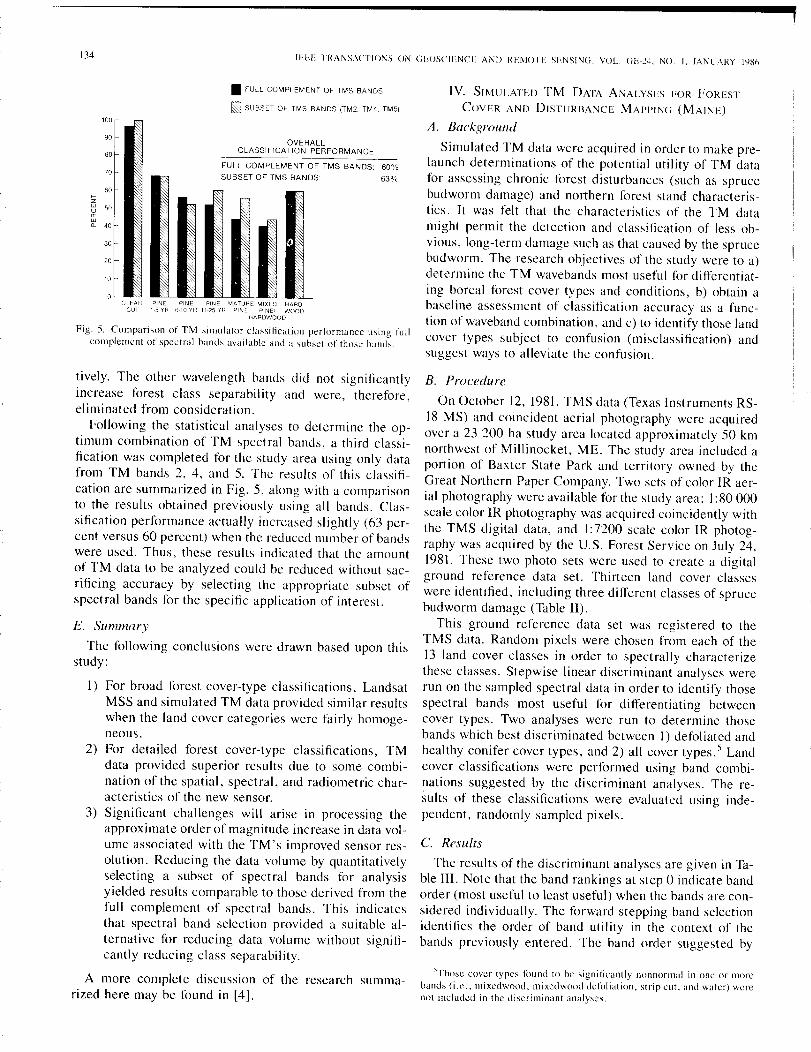
I:\4 IEEE TRANSACTlOI\S ON GEOSCIENCE AND REMOI E SENSING, VOL Gc:-~4, NO. I. JAI\UARY 1986
Fig. 5. Comparison of TM simulator classification perf<lrI11anCCusing fullcomplemcnt of spectral hands availablc and a subset of those bands.
• FULL COMPLEMENT OF TMS BANDS
~ SUBSET OF TMS BANDS (TM2, TM4, TM5)
70
60-c-tJ() 500:WCl. 40
30
20
10
OVERALLCLASSIFICATION PERFORMANCE
60%
63%
IV. SIMULATED TM DATA ANALYSES FOR FOREST
COVER AND DISTURBANCE MAPPING (MAI:'>iE)
A. Background
Simulated TM data were acquired in order to make pre-launch determinations of the potentia] utility of TM datafor assessing chronic forest disturbances (such as sprucebudworm damage) and northern forest stand characteris-tics. It was felt that the characteristics of the TM datamight permit the detection and classification of less ob-vious, long-term damage such as that caused by the sprucebudworm. The research objectives of the study were to a)determine the TM wavebands most useful for differentiat-ing boreal forest cover types and conditions, b) obtain abaseline assessment of classification accuracy as a func-tion of waveband combination, and c) to identify those landcover types subject to confusion (misclassification) andsuggest ways to alleviate the confusion.
tively, The other wavelength bands did not significantlyincrease forest class separability and were, therefore,eliminated from consideration.
Following the statistical analyses to determine the op-timum combination of TM spectral bands, a third classi-fication was completed for the study area using only datafrom TM bands 2, 4, and 5. The results of this classifi-cation are summarized in Fig, 5, along with a comparisonto the results obtained previously using all bands. Clas-sification performance actually increased slightly (63 per-cent versus 60 percent) when the reduced number of bandswere used. Thus, these results indicated that the amountof TM data to be analyzed could be reduced without sac-rificing accuracy by selecting the appropriate subset ofspectral bands for the specific application of interest.
E. Summary
The following conclusions were drawn based upon thisstudy:
]) For broad forest cover-type classifications, LandsatMSS and simulated TM data provided similar resultswhen the land cover categories were fairly homoge-neous.
2) For detailed forest cover-type classifications, TMdata provided superior results due to some combi-nation of the spatial, spectral, and radiometric char-acteristics of the new sensor.
3) Significant challenges will arise in processing theapproximate order of magnitude increase in data vol-ume associated with the TM's improved sensor res-olution. Reducing the data volume by quantitativelyselecting a subset of spectral bands for analysisyielded results comparable to those derived from thefull complement of spectral bands. This indicatesthat spectral band selection provided a suitable al-ternative for reducing data volume without signifi-cantly red\,;cing class separability.
A more complete discussion of the research summa-rized here may be found in [41.
B. Procedure
On October 12,1981, TMS data (Texas Instruments RS-18 MS) and coincident aerial photography were acquiredover a 23 200-ha study area located approximately 50 kmnorthwest of Millinocket, ME. The study area included aportion of Baxter State Park and territory owned by theGreat Northern Paper Company. Two sets of color IR aer-ial photography were available forthe study area; ]:80000scale color IR photography was acquired coincidently withthe TMS digital data, and I :7200 scale color IR photog-raphy was acquired by the U.S. Forest Service on July 24,1981. These two photo sets were used to create a digitalground reference data set. Thirteen land cover classeswere identIfied, including three different classes of sprucebud worm damage (Table II).
This ground reference data set was registered to theTMS data. Random pixels were chosen from each of the13 land cover classes in order to spectrally characterizethese classes. Stepwise linear discriminant analyses wererun on the sampled spectral data in order to identify thosespectral bands most useful for differentiating betweencover types. Two analyses were run to determine thosebands which best discriminated between I) defoliated andhealthy conifer cover types, and 2) all cover types. 5 Landcover classifications were performed using band combi-nations suggested by the discriminant analyses. The re-sults of these classifications were evaluated using inde-pendent, randomly sampled pixels.
C. Results
The results of the discriminant analyses are given in Ta-bie Ill. Note that the band rankings at step 0 indicate bandorder (most useful to least useful) when the bands are con-sidered individually. The forward stepping band selectionidentifies the order of band utility in the context of thebands previously entered. The band order suggested by
'Thosc cover typcs ICJUndto bc significantly nonnormal in one or morebands (i.t' .. mixedwood. mixedwood dct(Jliation. strip cut. and water) werenot included in the discriminant analyses.

WILLIAMS AND NELSON: REMOTELY SENSED DATA FOR ASSESSING FOREST STAND CONDITIONS 135
TABLE IILISTI"lG AND DESCRIPTION OF LAND COVER CLASSES FOU"lD IN GROU"lD
REFERENCE DATA SET FOR MAINE STUDY AREA
'\1I1Hht,[ oj
( ;r\llllld
I\'{l'l"t']l((' 1'1\1'1, !)e\CriptI01\
I (:I,'.ut'lit
Old Clean'li!<:()]lill'l*
ILudw()od"\11\/·<1 \\'()()d~
Bill.!:
- 1l1()H'd()\~'rl
'-j \\';t1t'l
(J <"'tr-ip \'Ilt
jo -'kado\\11 Se\l'H' <:()llilt",
])I,!()li,ltioll
12 111';\\"\ (,Olldt'l
Jkhdi~ltll)ll
l.\ \Ii\(,d \\o'lll
])l'!oli,tllilll
nl'J
IO·H7Itj.'j,)2
7:l:Hi1:>22,")hl02hl7{i
I 7·'-l1 Iii110.')0
3\11
2hhl
22'Jh
1'1l'l1"llllll.llltlv •.•Ll,h (HI gflllllll!
')(>1111' •.•hr-llll-hardw()(H! n')...';l'lwratlol1
'~(l/!; oj lilT ('10\\'11~llt'a i..•l'ol\iferoll\
·7()'i; 0111('(' ('lO\\'ll dn'a i...hardwood7()'i; IL,lId,\"()()d ,111(1 70(k '>\lftwood
\ldl'l .tlld ']1I-IIt'" IHlg ...l(]'; ,01 II,'!" ••l.uldiTlg, n'lllaillde!- 1>10\0,:11 down
Alpha level < 0.0I (4.0 F-·to-enter)
TABLE IIIRESULTS OF DISCRIMINANT ANALYSES FOR MAINE DATA SET
Forward Stepping Band Selection:Step 1 -- band 1 Step 3 -- band 5Step 2 u band 7 Step 4 -- band 3
Bands 2, 4, and 6 were not entered.
b. A1LQQyer Types:
Cover tYl(es considered: All co~er types listed in Table 2except mIxedwood, mixedwood defolIation, stripcut, and water.
coniferous defoliation were confused with each other andto a limited extent with blowdown. Evidently the TMSdata could not be used to distinguish detailed canopy clo-sure classes. However, TMS data did permit the delinea-tion of mixedwood defoliation from the pure conifer dam-age. Meadows (grassland) were classified very poorly, inpart due to the small areal extent of the grassy areas, cou-pled with minor misregistration problems between theTMS data and the digitized photointerpretation results.Hardwoods, which are often spectrally similar to grass-lands, were confused with meadow; however, the greatestsource of hardwood misclassification error was the mixed-wood defoliation category. This situation may be an arti-fact of the October 12 data collection date. Hardwoodleaves had begun to drop, and the hardwood cover typeexhibited a great deal of spectral variability due to fall leafcoloration. On the basis of these results, the following ob-servations were made:
5. band 3 f89.8l6. band 5 66.67. band 2 50.4
informative to least informativeBand Ranking at Step 0, most(F-to-enter in parentheses):
I. band 4 t178.Oj2. band 7 176.83. band I 175. I4. band 6 146.7
a. Defolii!!~!Land Hef!lt~.Q!1j,J~LQQve~~:
Cover types cons i dered:healthy coniferheavy conifer defoliationsevere conifer defoliation
Alpha level <0.05 (4.0 F-to-enter)Band Ranking at Step 0, most informative to least informative(F- to~enter in parentreseSj:I. band I 57.3 5. band 5 f22.0J2. band 7 45.2 6. band 3 8.6)
3. band 4 27.7) 7. band 2 6.5)4. band 6 23.9)
the results of the forward stepping discriminant analyses(all cover types) was used to determine the effects of ad-ditional spectral bands on classification accuracy. Ananalysis of the best single band, the best two bands, bestthree, four, ... , seven bands showed that test pixel clas-sification accuracy did not increase with the inclusion ofthe sixth and seventh bands. When the best five TMSbands were used to classify the scene and test pixel ac-curacies were calculated, the overall classification accu-racy was 57.7 percent (TMS classification results com-pared with photointerpreted ground reference data). Thefive TMS bands which were used were the blue (TM I),red (TM3), near infrared (TM4), and two middle infraredbands (TM5 and TM7). Table IV reports the individualland cover classification accuracies using these bands.
The land cover clas';ification results in Table IV exhibita wide range of accuracies. Severe (80-100 percent can-opy removed) and heavy (60-80 percent canopy removed)
Forward Stepping Band Selection:Step 1 -- band 4Step 2 -- band 1Step 3 .- band 5
Band 2 was not entered.
Step 4 -- band 7Step 5 .- band 3Step 6 ..- band 6
I) The discriminant analyses suggested that usefulwaveband combinations include at least one bandfrom the visible (0.4-0.7 Jlm), near infrared (0.7-1.3Jlm), and middle infrared (1.3-3.0 Jlm) spectral re-glOns.
2) The blue band (TMl) proved to be the most usefulfor discriminating coniferous defoliation categories.The forward stepping selection process ranked theblue band second in overall utility for assessing allcover types.
3) The two middle infrared bands (TM5 and TM7) pro-vided significant spectral information for differen-tiating all cover type groups considered. TM7 provedmost useful for coniferous defoliation assessment,while TM5 proved most useful for differentiating allcover types. The two middle infrared bands do notappear to contain redundant information. The dis-criminant analyses indicate that TM4 and TM7 con-tain redundant information since the inclusion of onein the discriminant function precludes or delays theinclusion of the second (compare Step 0 results tothe forward stepping results (Table III).
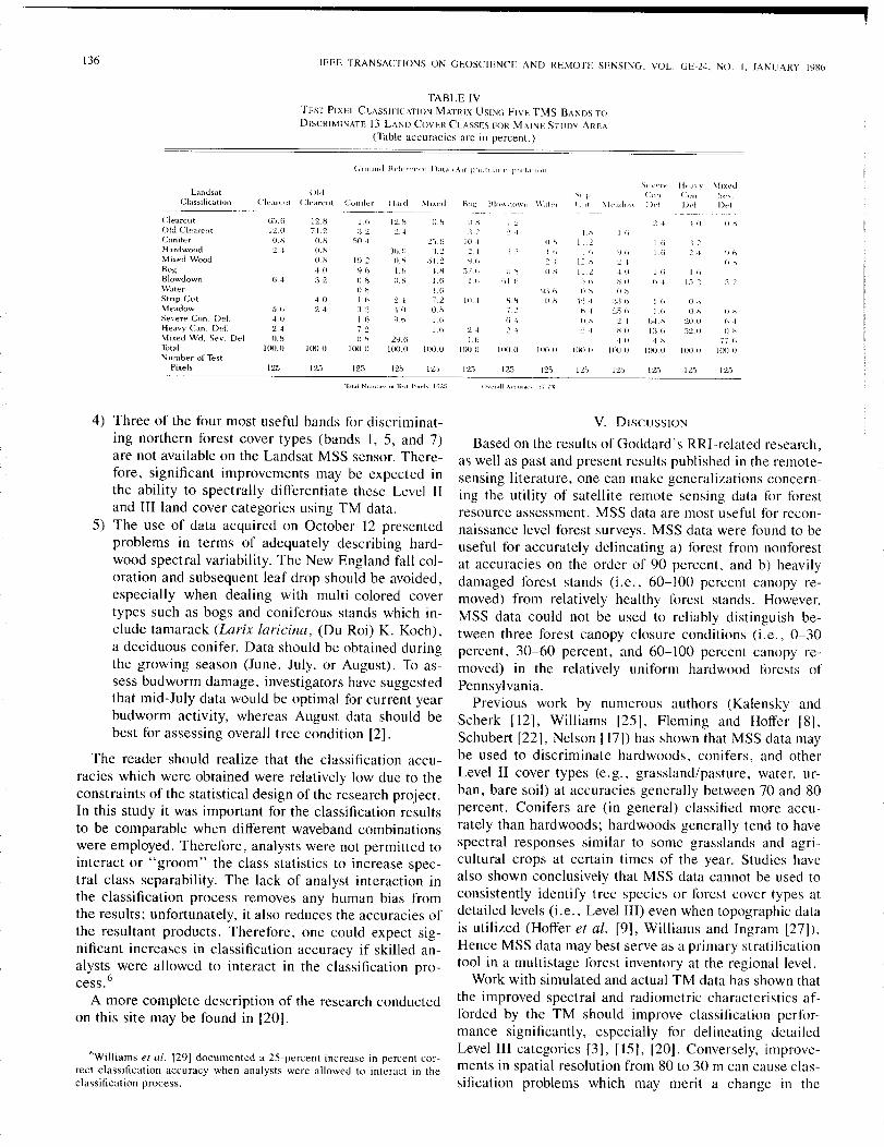
136
LanusatClassification
ClearcutOld Creare-tltConiferHardwood.\1 ixed WoodBogSlowdown\VaterStrip Cut\leadowSevere COil DeLHeavy Can. I)ef.Mixed Wd. Sev Del'TotalNumber nfTest
Pixels
IEEE TRANSACTIONS ON GEOSCIENCE AND RE:-'IOTE SEI\SING. VOL. G1O-24. NO. I. JANUARY 19X6
TABLE IVTEST PIXEL CLASSIFICATION MATRIX USING FIVE TMS BMms TO
DISCRIMINATE 13 LAND COVER CLASSES FOR MAINE STUDY AREA
(Table accuracies are in percent.)
\('\'('rt' Ift,,!\\ \liXl·dOld Slip (:011 (:011 Sn
Clearcut Clearclll Co[]ifel Hard \-1lxed Bo~ Hiowdowli \\';ll,'[ (:lIt \kadll\\ Del 1)l'l I)t>f
6.5.6 12.H 1.6 12.S OH OK ~:2 2 ..~ j () (l.i-l12,(1 71.2 :3 2 2.-t 1 2 :2 .j L·'" I h
OH O.H SIU 25() 10 .J 0'1 112 If] I :22,-1 O.H 36.0 3.2 2-1 1 :2 )ti I f. ~U) l.f; :2 ·1 l},h
OH 19.2 O.S SI.2 Y,() 2 I 12 , 2·' Ii ,4.0 96 1.6 U 57h () ., () ., 112 J 0 If; III
6.4 .32 OS OH 1.6 I.h (-iJb S(j ,~o (l·t 1.'1 :2 ] 2OK 1.!-1 CjJ() OS 01';.
4.0 I (; 2 ·1 7.2 10 4 SH 0 .' .t2·\ ::n,b I 6 o H5.6 2.·t '32 ·1.(1 OH -, tit 2.') r. 1.6 OK 0 "4.0 16 Q,6 1.6 (i~ OS 2·1 64_,~ 20.0 fi I21 7'2 lfi 21 2·1 :2 ,f kO J3ti ,'>20 <I HO.H 0,11 29,{) 1.f., L(l 4 K " h
I()()O J(X) 0 J(Xl.O J(X)() J(X)O J(XI () loo.n J(Kl () WOO 11K) 0 J(Xl() 11K) 0 J(Kl <I
125 12.5 125 12.5 125 125 12.5 12,':. 12,5 125 125 12.5 125
l'.t,,1 N"mb•., ,,('Ii·,l 1',••. 1, 1(2) (h"",11 A,~'",,,,,, ,')77'1;
4) Three of the four most useful bands for discriminat-ing northern forest cover types (bands 1, 5, and 7)are not available on the Landsat MSS sensor. There-fore, significant improvements may be expected inthe ability to spectrally differentiate these Level IIand III land cover categories using TM data.
5) The use of data acquired on October 12 presentedproblems in terms of adequately describing hard-wood spectral variability. The New England fall col-oration and subsequent leaf drop should be avoided,especially when dealing with multi-colored covertypes such as bogs and coniferous stands which in-clude tamarack (Larix laricina, (Du Roi) K. Koch),a deciduous conifer. Data should be obtained duringthe growing season (June, July, or August). To as-sess budworm damage, investigators have suggestedthat mid-July data would be optimal for current yearbudworm activity, whereas August data should bebest for assessing overall tree condition [2].
The reader should realize that the classification accu-racies which were obtained were relatively low due to theconstraints of the statistical design of the research project.In this study it was important for the classification resultsto be comparable when different waveband combinationswere employed. Therefore, analysts were not permitted tointeract or "groom" the class statistics to increase spec-tral class separability. The lack of analyst interaction inthe classification process removes any human bias fromthe results; unfortunately, it also reduces the accuracies ofthe resultant products. Therefore, one could expect sig-nificant increases in classification accuracy if skilled an-alysts were allowed to interact in the classification pro-cess.6
A more complete description of the research conductedon this site may be found in [20].
"Williams et ai. 129] documented a 25-percent increase in percent cor-rect classification accuracy when analysts were allowed to interact in theclassification process.
V. DISCUSSION
Based on the results of Goddard's RRI-related research,as well as past and present results published in the remote-sensing literature, one can make generalizations concern-ing the utility of satellite remote sensing data ft1r forestresource assessment. MSS data are most useful for recon-naissance level forest surveys. MSS data were ft1Undto beuseful for accurately delineating a) forest from nonforestat accuracies on the order of 90 percent, and b) heavilydamaged forest stands (i.e., 60-100 percent canopy re-moved) from relatively healthy forest stands. However,MSS data could not be used to reliably distinguish be-tween three forest canopy closure conditions (i.e., 0-30percent, 30-60 percent, and 60-100 percent canopy re-moved) in the relatively uniform hardwood forests ofPennsylvania.
Previous work by numerous authors (Kalensky andScherk [12], Williams [25], Fleming and Hoffer [8],Schubert [22], Nelson fl7]) has shown that MSS data maybe used to discriminate hardwoods, conifers, and otherLevel II cover types (e.g., grassland/pasture, water, ur-ban, bare soil) at accuracies generally between 70 and 80percent. Conifers are (in general) classified more accu-rately than hardwoods; hardwoods generally tend to havespectral responses similar to some grasslands and agri-cultural crops at certain times of the year. Studies havealso shown conclusively that MSS data cannot be used toconsistently identify tree species or forest cover types atdetailed levels (i.e., Level III) even when topographic datais utilized (Hoffer et at. [9], Williams and Ingram [27]).Hence MSS data may best serve as a primary stratificationtool in a multistage forest inventory at the regional level.
Work with simulated and actual TM data has shown thatthe improved spectral and radiometric characteristics af-forded by the TM should improve classification perfor-mance significantly, especially for del ineating detailedLevel III categories [3], [15], [201. Conversely, improve-ments in spatial resolution from 80 to 30 m can cause clas-sification problems which may merit a change in the
WILLIAMS AND NELSON: REMOTELY SENSED DATA FOR ASSESSING FOREST STAND CONDITIONS 137
"standard" approaches to classifying a scene. Studieswhich have used TM or TMS data on forested study siteshave produced classification accuracies higher than, equalto, or below equivalent MSS data products [4], [10], [13J,[29]. The effects of changing spatial resolution on classi-fication accuracy are discussed and quantified by Mark-ham and Townshend [14] and Irons et al. [11]. Evidentlydigital image processing techniques must be revised in or-der to handle the spatial and spectral information availablein TM data. The information content of the TM data farexceeds that of MSS data, as evident in a visual compar-ison of MSS and TM imagery.
The remote sensing research community is now facedwith the problem of devising algorithms to efficiently ex-tract information from TM data. Until such techniques aredeveloped, photointerpretation of TM image products maybe of most immediate benefit to foresters. The imageryhas many of the qualities of high-altitude small-scale(1:100 000 +) aerial photography. TM photo products,which are available in black and white, true color, andfalse color infrared, may be used to identify clearcuts, stripcut areas (with strips being only one chain wide, :::::20m), water, bare soil, roads, and, most likely, hardwoodand softwood stands. The quality of the small-scale im-agery, the synoptic coverage, and the cost of the productbehooves potential users to investigate the use of TM im-agery if plans are being made to fly a high-altitude recon-naissance mission.
In summary, it is apparent that we now have the capa-bility to assess forest resources on local, regional, andcontinental scales using data from sensors currently inEarth orbit. There are distinct trade-offs associated withdata acquired by different sensors, and the research con-ducte9 in support of the Renewable Resources Inventoryproject helped to develop a better understanding of theapplicability of satellite data for forest resource assess-ment.
REFERENCES
II] AgRISTARS, Renewable Resources Inventory Implementation Plan.NASA/Lyndon B. Johnson Space Center, Houston, TX, 1979.
[2] M. D. Ashley, J. Rea, and L Wright, "Spruce bud worm damage eval-uations using aerial photography," Photogrammelr. Eng., vol. 42, no.10, pp. 1265-1272, 1976.
[3] M. K. Butera" A correlation and regression analysis of percent can-opy closure vs. TMS spectral response for selected forest sites in theSan Juan National Forcst, Colorado," in Proc. AgR1STARS Symp.NASA/Johnson Space Center, Houston, TX, 1982.
[4] C. L. Dottavio and D. L. Williams, "Mapping a southern pine plan-tation with satellite and aircraft scanner data: a comparison of presentand future Landsat sensors," 1. Appl. Photographic Eng, vol. 8, no.I, pp. 58-62, 1982.
(5] C. L. Dottavio and D. L. Williams, "Satellite technology: An im-proved means for monitoring forest insect defoliation," 1. Forestry,vol. 81, no. I, pp. 30-34, 1983.
[6] C. L. Dottavio, R. F. Nelson, and D. L. Williams, "Final Rcport:Monitoring the defoliation of hardwood forests in Pcnnsylvania usingLandsat," NASA/Goddard Space Flight Center, Greenbelt, MD, 1983.
[7] IDIMS Functional Guide, vol. I, Electromagnetic Systems Lab. Sun-nyvale, CA, 1982.
[8] M. D. Fleming and R. M. Hoffer, "Computer-aided analysis tech-niques fin an operational system to map forest lands utilizing LandsatMSS data," Lab. Applications of Rcmote Sensing, Purdue Univ., WcstLafayette, IN, Tech. Rep. 112277, 1977.
19] R. M. Hoffer, M. D. Fleming, L. A. Bartolucci, S. M. Davis, and R.F. Nelson, "Digital processing of Landsat MSS and topographic datato improve capabilities for computcrized mapping of forest covertypes," Lab. Applications of Remote Sensing, Purdue Univ., WestLafayette, IN, Tech. Rep. 011579, 1979.
1101 R. M. Holfer, M. E. Dean, D. J. Knowlton, and R. S. Latty, "Eval-uation of SLAR and simulated Thematic Mapper data fin forest covermapping using computer-aided analysis techniques," Lab. Applica-tions of Remote Sensing, Purdue Univ" West Lafayette, IN, Tech.Rep. 083182, 1982.
[II( J. R. Irons, B. L. Markham, R, F. Nelson, D. L. Toll, D. L. Wil-liams, R. S. Latty, R. L. Kennard, and M. L. Stauffer, "The effectsof scnsor advancements on Thematic Mapper data classification," inProc. 18th Int. Symp. Remote Sensing Environment (Paris, France),pp. 1759-1773, 1984,
112) Z. Kalensky and L. R. Scherk, "Accuracy of forest mapping fromLandsat computer compatible tapes," in Proc. IOlh Inl. Symp. RemoleSensing I!l Environment, vol. II, ERIM (Ann Arbor, MI), pp, 1159-1167, 1975.
[13) R. S. Latty and R, M. Hoffer, "Computer-based classification accu-racy due to the spatial resolution using per-point and per-field classi-fication techniques," in Proc. Machine Processing of Remolely SensedDala Symp. (West Lafayette, IN), pp, 384-392, 1981.
[14] B. L. Markham and J. R. G. Townshend, "Land cover classificationaccuracy as a function of sensor spatial resolution," in Proc. 151h Int.Symp. Remole Sensing Environment (ERIM, Ann Arbor, MI). pp.1075-1090, 1981.
[15] "A prospectus for Thematic Mapper research in the earth sciences,"NASA/Goddard Space Flight Center, Greenbelt, MD, NASA Tcch.Memo 86149, ]984.
[16] R. F. Nelson, "Defining the temporal window for monitoring forestcanopy defoliation using Landsat," in Proc. ASP-ACSM Meel., Tech.Pap. (Washington, DC). pp. 367-382, 1981.
[17J R. F. Nelson, "A comparison of two methods for classifying forest-land," Int. J. Remote Sensing, vol. 2, no. I, pp. 49-60, 1981.
[181 R. F. Nelson, "Detecting finest canopy change using Landsat,"NASA/Goddard Space Flight Center, Greenbelt, MD., AgRISTARSFinal Rep. RR-62-04258, 1982.
119] R. F. Nclson, "Detecting forest canopy change due to insect activityusing Landsat MSS," Photogrammetr. Eng., vol. 49, no. 9, pp. 1303-1314, 1983.
[20] R. F. Nelson, R. S. Latty, and G. Molt, "Classifying northern forestsusing Thematic Mapper simulator data," Photogrammetr. Eng., vol.50, no. 5, pp. 607-617, 1984.
121] S. A. Russo and M. L. Stauffer, "The statewide finest/non-forestclassification of Pennsylvania using Landsat MSS data," NASA/God-dard Space Flight Center, Greenbelt, MD, CSC/TM-83/6073, Contr.Rep., NAS5-24350, 1983.
1221 J. S. Schubert "The Canada land inventory~Computer processing ofLandsat data for Canada land inventory land use mapping," GregoryGeosciences Ltd., Ottawa, Ontario, Rep. 13, 1978.
123] C. J. Tucker "A comparison of satellite sensor bands for vegetationmonitoring," Photowammetr. Eng" vol. 44, no. II, pp. 1369-1380,1978.
124J B. J. Turner and D. L. Williams, "The ORSER Landsat data base ofPennsylvania," in Proc. Nat. Conf Energy Res. Managemenl, vol. 1(Baltimore, MD), pp. 149-160, 1982.
[25] D. L. Williams, "A canopy-related stratification of a southern pineforest using Landsat digital data," in Proc. ASP Fall Conv. (Seattle,WA). pp. 231-239, 1976.
126J D. L. Williams and M. L. Stauffer, "What can the forestry commu-nity expect from Landsat-D Thematic Mapper data'?" in Proc. Symp.Remole Sen.l·illg of Nal. Res. (Univ. of Idaho, Moscow, 10), pp. 475-492, 1979.
[27) D. L. Williams and K. J. Ingram, "Integration of digital elevationmodel data and Landsat MSS data to quantify the effects of slope ori-entation on the classification of [()rest canopy condition," in Proc. 71hInt. Symp. Machine Proc. Remotely Sensed Data (Purdue Univ., WestLafayette, IN), pp. 352-362, 1981.
1281 D. L. Williams, C. L. Dottavio, and R. F. Nelson, "Development ofa statewide Landsat digital data base for forest insect damage assess-ment," in Proc. Aulo-Carto 5/1SPRS IV Symp. (Crystal City, VA), pp.191-203. 1982.
129] D. L. Williams, J. R. Irons, B. L. Markham, R. F. Nelson, D. L.Toll, R. S. Latty, and M. L. Stauffer, "A statistical evaluation of theadvantages of Landsat Thematic Mapper data in comparison to Mul-
138 IEEE TRANSACT/OKS ON GEOSCIENCE AND REMOTE SENSING, VOL, GE-24, NO, L JANUARY In6
tispeetral Scanner data," IEf,'/:,' '/raf/s, Ceosci. Remole Sellsif/K, vol.GE-22, no, 3, pp, 294-302, 1984,
130] D, L Williams, R, F, Nelson, and C. L Dottavio, "A georeferenccdLandsat digital database for fClrcst insect-damage assessment," 1/1/, Jo{Remole Sef/siIlK, vol. 6, no, 5, pp, 643-656, 1985,
*Darrel L. Williams received the B,S, and MSdegrees in I()rest science from the PennsylvaniaState University in ]973 and 1974, respectively,He is currently working toward the Ph,D, degreein biogeography and remote sensing at the Uni-versity of Maryland,
He has been employed as a Physical Scientist inthe Earth Resources Branch, Laboratory for Ter-restrial Physics, NASA Goddard Space FlightCenter, since 1975, His research at Goddard hasinvolved the development of techniques to enhance
the utility of digital remotely sensed data IClrassessing the filrest canopy,He served as Landsat-4 Assistant Project Scientist from ]979 through 1983,
*Ross 1<'. Nelson received the B,S, degree in forestmanagement in 1974 from the University of Maine,Orono, and the M,S, degree in IClfestry/remotesensing in 1979 from Purdue University,
As a Physical Scientist in the Earth ResourcesBranch at tbe NASA Goddard Space Flight Centersince 1979, he has been involved with the use ofdigital remotely sensed data for assessing the fc)r-cst canopy, He has worked with Landsat MSS datato evaluate gypsy moth damage, Thematic Map-per Simulator data to evaluate spruce bud worm
damage, and AYHRR and MSS data to assess delc)restation in South Amer-ica, He has worked with geobotanieal scientists to determine the eflects ofmineralization on J()rest canopy condition, and is investigating the utilityof laser-induced fluorescence for tree species identification,
IEEE TRANSACTIONS ON GEOSCIENCE AND REMOTE SENSING. VOL. GE-24. NO. I. JANUARY 1986 139
Coniferous Forest Classification and Inventory UsingLandsat and Digital Terrain Data
JANET FRANKLIN, THOMAS L. LOGAN, CURTIS E. WOODCOCK, ANDALAN H. STRAHLER
Abstract-Accurate cost-effective stratification of forest vegetationand timber inventory is the primary goal of a Forest Classification andInventory System (FOCIS) developed at the University of California,Santa Barbara, and the Jet Propulsion Laboratory, Pasadena. Conven-tional timber stratification using photointerpretation can be time-con-suming, costly, and inconsistent from analyst to analyst. FOCIS wasdesigned to overcome these problems by using machine-processing tech-niques to extract and process tonal, textural, and terrain informationfrom registered Landsat multispectral and digital terrain data. FOCISwas developed in northern California's Klamath National Forest (KNF),where the rugged terrain and diverse ecological conditions provided anexcellent area for testing Landsat-based inventory techniques. The FO-CIS procedure was further refined in the Eldorado National Forest(ENF), where the portability and flexibility of I<-OCIS was verified.
Using FOCIS as a basis for stratified sampling, the softwood timbervolume of the western portion of the Klamath (944 833 acres; 422 340ha) was estimated at 3.83 x 10⁹ fe (1.08 x lOR m3), with a standarderror of 4.8 percent based on 89 sample plots. For the Eldorado, thesoftwood timber volume was estimated at 1.88 x 10⁹ fe (0.53 x lOR m3
)
for an area of 342 818 acres (138 738 ha) with a standard error of 4.0percent, based on 56 sample plots. These results illustrate the power ofFOCIS methods to produce timely accurate large-area inventories withcomparable accuracies and reduced costs when compared to conven-tional timber inventory methods.
Key Words-Classification, timber inventory, digital terrain data,forest vegetation, Landsat.
I. INTRODUCTION
INFORESTRY and range science, the need often arisesto sample and inventory natural vegetation. Conven-
tional methods use manual interpretation of aerial photog-raphy to delineate areas of homogeneous vegetation(termed stands) using attributes of image tone, texture,and topography. Stands with like attributes are thengrouped into strata from which samples are drawn to yieldinventory data that describe attributes of interest of thenatural vegetation. Because this process is based on man-ual photointerpretation, it can be time-consuming andcostly, as well as inconsistent from analyst to analyst. In
Manuscript received May 8, 1985; revised July 18.1985. This work wassupported by NASA under Contract NAS-9-15509, by the USFS-UCSB un-der Join, Agreement 37, by the USFS under Contract 53-91S8-0-6362, andby the California Institute of Technology's President's Fund, Award PF-123, under NASA Contract NAS-7-100.
J. Franklin is with the Department of Geography, University of Califor-nia, Santa Barbara, CA 93106.
T. L. Logan is with the Jet Propulsion Laboratory, California Instituteof Technology, Pasadena, CA 91103.
C. E. Woodcock is with the Department of Geography. Boston Univer-sity, Boston, MA 02215.
A. H. Strahler is with the Department of Geology and Geography, HunterCollege of the City University of New York, New York, NY 10021.
IEEE Log Number 8406237.
this paper we describe an automated system for natural-vegetation inventory which utilizes digital image process-ing of multispectral Landsat data and registered digitalterrain information, This technology, referred to as theForest Classification and Inventory System (FOCIS), hasshown the capability to classify and stratify forest vege-tation for timber-volume inventory as precisely and morecost-effectively than conventional methods of manual pho-tointerpretation.
An earlier article discussed the general nature of theproblem of stratifying registered digital terrain and Land-sat data for timber and rangeland inventory, and includeda brief review of FOCIS procedures as they existed at thattime [1]. This article focuses on some of the more impor-tant procedural steps in FOCIS, and describes the accu-racy of timber inventories of the Klamath and EldoradoNational Forests using FOCIS procedures. Technical de-tails concerning the information-extraction process can befound in our technical reports [2], [3].
Thus far, FOCIS presents the only example of a fullyintegrated methodology for conducting large-area timberinventory using satellite and DTM data, although a num-ber of studies have employed Landsat data (and, for some,digital terrain data as well) in forest cover type mapping[4]-[7]. Unfortunately, an extensive review of the variousapproaches that have been utilized is beyond the scope ofthis paper.
II. BACKGROUNDA. Conventional Methodology for Timber- VolumeInventory
To provide a background for the description of FOCIS,we will summarize the conventional methodology used toproduce timber volume estimates by Region 5 (California)of the U.S. Forest Service. Timber inventory is executedin three steps: stand mapping, stratification, and samplecollection and data processing.
Foresters skilled in air photo interpretation use conven-tional resource photography to delineate timber stands bydrawing boundaries around areas of uniform vegetation ofat least 10 acres (4 ha) in size. I These stand boundariesare transferred from the air photos to 7~-min topographicquadrangles, and labels are affixed to each stand indicat-
ISince American forestry still uses English units, this research wasplanned and carried out in the English system. Accordingly, English unitsare shown first with metric equivalents in parentheses.
0196-2892/86/0100-0139$01.00 © 1986 IEEE
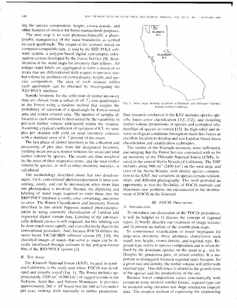
------------------------------------ ...,140 1I~.Lf'TRANSACTIONS i)~ (;EOSCII,M'E AND REMOTE SL~SIN(;, VOL. (;[':-24, \Ii). I, JANI!ARY 19H6
ing the species cOmposItIon, height, crown density, andother features of interest for forest-management purposes.
The next step is to scan photomechanically a photo-graphic transparency of the stand boundaries as scribedon each quadrangle. Thc output of the scanner, stored oncomputer-compatible tape, is read by the RID*POLY soft-ware system, a polygon-based digital cartographic infor-mation system developed by the Forest Service 181, Strat-ification of the stand maps for inveutory then follows. Allunique stand labels arc aggregated to form a dozen or .sostrata that arc differentiated with respect to per-acre tim-ber volume by attributes of crown density, height, and spe--cies composition. The area of each stratum withineach quadrangle can be obtained by interrogating theRID*POLY database.
Sample locations for the collection of timber-inventorydata are chosen from a subset of all 7 ~-Illin quadranglesin the Forest using a random method that weights theprobabi Iity of selection of a quadrangle by Forest -ownedarea and within-stratum area, The number of samples al-located to each stratum is determined by the variability inper-acre timber volume anticipated within the stratum,Assuming a typical coefficient of variation of 0.5, six sam-ples per stratum will yield an areal inventory estimatewith a standard crror of 6-7 percent of the mean.
The last phase of timber inventory is the collection andprocessing of plot data from the designated locations,yielding mean per-·acre timber volumes fiJr strata and totaltimbcr volume by species. Thc means are then weightedby the areas of their respective strata, and the total timbervolume by species, as well as other inventory statistics. iscalculated.
The methodology described above has two disadvan-tages. First, conventional photointerpretation is timc con-suming, costly, and can be inconsistent when more thanone photoanalyst is involved. Second, the digitizing andlabeling of stand maps required to enter them into theRID*POLY database is costly, time consuming, and proneto error. The Forest Classification and Inventory Systemdescribed in this article bypasses manual photointerpre-tation by using automatic classification of Landsat andregistered digital terrain data. Labeling of the automati-cally defined classes is still required, but this labeling canbe done much more rapidly and cost-effectively than in theconventional procedure. And, because FOCIS utilizes theraster-based VICAR/IBIS software system 19], [101, theclassified images of stands that serve as maps can be di-rectly interfaced through software to the polygon-]iOlflllatfiles of the RID*POLY system 13].
B. Test Areas
The Klamath National Forest (KNF). located in uorth-ern California, is the study area wherc FOCIS was dcvel-oped and initially tested (Fig. I). The Forest includcs ap-proximately 2500 mi" (6700 km2
) of rugged terrain in theSiskiyou, Scott Bar, and Salmon Mountains. It provillcsapproximately 260 x 10') board-feet (61 00(1111) oftimhcrper year, ranking sixth nationally in timber production.
Fig. I Index IIlap sh<l\ving locations 01 Klamalh and Eldorado "\ationalFor"st, WIthin California.
Past research conducted in the KNF includes species-spe-cific forest cover classification Ill], [12/, and modelingtimber-volume proportions of species and ecological rela-tionships of species to terrain [13]. Its high relief and di-verse ecological conditions throughout made this Forest anexcellent location to dcvelop and test Landsat-based forestclassihcation and stratification techniques.
The results of the Klamath inventory were sufficientlyencouraging that the Forest Service contracted with us foran inventory of the Eldorado National Forest (ENF), lo-cated in the central Sierra Nevada of California. The ENFincludes about 900 mi" (2400 km2
) on the west slope andcrest of the Sierra Nevada, with similar species composi-tion to the KN F, but variations in species-terrain relation-ships, and different physiography. This work provided anopportunity to test the tlexibility of FOCIS methods andilluminate new problems not encountered in the develop-ment of FOCIS in the Klamath.
III. FOCIS PROCEDUREA. Introduction
To introduce our discussion of the FOCIS procedures,it will be helpful to I) discuss the concept of regionaltypes; 2) briefly describc our treatmcnt of image texture;and 3) prescnt an outline of the stratification steps.
In conventional stratification of tilrest vegetation forlarge-area inventory, thrce attributes characterize eachstand: tree height, crown density, and regional type. Re-gional type refers to species composition and is often de-fined by the dominant spccies on the stand (e.g., red fir,Douglas fir, pondcrosa pine, or mixed conifer), It is im-portant to distinguish between regional types because, fora givcn size and density, the timber volume will differ withregional type. This difference is related to the growth formof the species and the productivity of the site.
Because forest composition varies systematically withterrain in many western conifer f(,rests, regional type canbe modeled using elevation and slope orientation (aspect)data, The simplest method of expressing the relationship

FRANKLIN et al.: FOREST CLASSIFICATION AND INVENTORY SYSTEM141
1000 ~-L-_. I I ..~_-----L..------L-........JI 8 .6 4 2 0 ~2 ~4 ~,6 ~,8 ~I
COSINE OF ASPECT
Fig. 2. Regional~type field graph for Doggett Natural Region, Klamath N~~tional Forest. Points plot 'regional type as observed In the field: red fir(circles). mixed conifer (X 's), and ponderosa/Jeffrey pine. Lines dlVldeelevation/aspect space into areas associated with the three regIonal types.(Note: triangles on lower right above lower line denote pine sItes.on ser~pentine. which are atypical of the region as a whole and were Ignoredwhen fitting the line.)
other areas [151-[171, and is documented in the Klamathand Eldorado by our regional type graphs (discussed in afollowing section).
C. Modeling Regional rvpe Using Digital Terrain DataObservations in the Klamath, Eldorado, and other west-
ern coniferous forest areas have shown that forest com-position typically varies systematically with topography,responding regularly to changes in elevation and slope as-pect. Aspect tends to influence elevational relationships;north to northeast exposures are typically more favorablefor tree growth than drier southwestern exposures, so thatspecies exhibiting elevational zonation tend to occur atlower elevations on northeast-facing slopes.
Regional type is a level of classification used by the U.S.Forest Service to divide forests into broad categories basedon species composition. In the Klamath, four regionaltypes were recognized: red fir (R), mixed conifer (M),Douglas fir (D), and ponderosa/Jeffrey pine (P); In theEldorado, only three were present: red fir, mixed conifer,and subalpine conifer (SA). The subalpine type was foundin the Eldorado only within the Desolation Wildernessarea. Although this type was mapped, no samples wereallocated to it since harvesting is not possible within thewilderness area. Consequently, timber volume calcula-tions omitted this type.
Field graphs were used to model regional type from thedigital terrain data (Fig. 2). To construct the field graphs,elevation, aspect, and regional type were observed at lo-cations chosen to represent the full range of the elevation-aspect combinations. Types were then plotted by elevationand by cos (aspect-45°). Lines fitted by eye partitionedthe elevation-aspect measurement space into areas repre-senting each regional type.
Functions defining those lines were input to a VICARimage-processing program to determine the most likely
between elevation, aspect, and regional type involves sys-tematically observing regional type at all aspects and el-evations, and plotting regional type on a graph with ele-vation and the cosine of aspect as axes. The regional typeof any point on the ground can thus be predicted by de-termining the elevation and aspect of the point and thenconsulting the graph. This procedure is discussed in moredetail in a following section.
The FOCIS automated stratification procedure uses thesame three characteristics oftone, texture, and terrain thatthe photointerpreter uses in delineating timber stands.Landsat multispectral reflectance data provide tonal andtextural information and digital elevation models providethe required terrain information.
Classification of the Landsat and texture data into size-and-density-based strata using FOCIS is accomplished inthe following steps2:
1) unsupervised clustering;2) statistical editing;3) classification using a hybrid parallelepiped/maxi-
mum-likelihood classifier;4) differential illumination compensation; and5) spatial-spectral editing and labeling of strata.
This basic procedure was refined in the ENF to include:
6) iterative clustering, classification, and editing; and7) spatial simplification to provide a stand map with
stands of a minimum areal extent.
B. Digital Terrain ProcessingDigital terrain data for the Klamath and Eldorado Na-
tional Forests were obtained from the National Carto-graphic Information Center. For the Klamath, data wereof the DMA series, produced by scanning of 1: 250 000contour maps. For the Eldorado, Digital Land Mass Sim-ulator data were used. In this type of digital terrain model,an elevation is provided for each 3-s interval on a geo-graphic grid. In the Klamath, terrain data were registeredto the Landsat image using a geometric resampling algo-rithm that employs a two-dimensional correction grid de-rived from control points. In the Eldorado, Landsat andterrain data were each registered to Universal TransverseMercator projection using a similar procedure.
After registration of the Landsat and terrain data, sep-arate images of slope angle and aspect were generatedfrom elevation by the least squares fitting of a planethrough each pixel and its four nearest neighbors. The as-pect image was then transformed using a cosine tra.nsfor-mation with a shifted axis, following the suggestIOn ofHartung and Lloyd [141. The transformation was: cos (as-pect -45 0). This function is based on the ecological obser-vation that sites on northeast-facing slopes are most pro-ductive, those on southwest-facing slopes are leastproductive, and those on southeast and northwest slop~sare intermediate. This phenomenon has been observed III
2Except as noted. the procedures discussed below are the same for theKlamath and Eldorado National Forests.
7000
6000
f- 5000wWLL
~zQf-
§W--lW
2000
) .) 0"
0Red Fir 0 8 'J:)
0 ~,g; x
0
g; ®x
, ie,
XXx
xx x~x x
Mixed Coniferx
'x
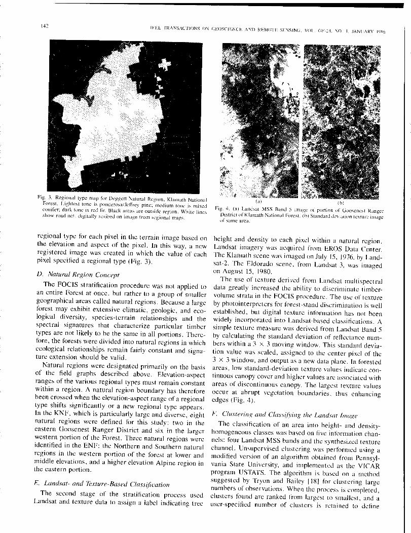
142IEEE TRANSACTIONS ON CiEOSCIENCE AND RhMOTE SENSING, VOL, GF24, NO. L JANUARY 19X6
Fig, 3, Regional-type map fe)r Doggett Natural Region, Klamath NationalForesl. Lighlest tone is ponderosa/Jeffrey pine: medium tone is mixedconifer: dark tone is red fir. Black areas are outside region. White linesshow road net, digitally scribed on image from regional maps.
regional type for each pixel in the terrain image based onthe elevation and aspect of the pixel. In this way, a newregistered image was created in which the value of eachpixel specified a regional type (Fig. 3).
D. Natural Region Concept
The FOCIS stratification procedure was not applied toan entire Forest at once, but rather to a group of smallergeographical areas called natural regions, Because a largeforest may exhibit extensive climatic, geologic, and eco-logical diversity, species-terrain relationships and thespectral signatures that characterize particular timbertypes are not likely to be the same in all portions. There-fore, the forests were divided into natural regions in whichecological relationships remain fairly constant and signa-ture extension should be valid.
Natural regions were designated primarily on the basisof the field graphs described above. Elevation-aspectranges of the various regional types must remain constantwithin a region. A natural region boundary has thereforebeen crossed when the elevation-aspect range of a regionaltype shifts significantly or a new regional type appears.In the KNF, which is particularly large and diverse, eightnatural regions were defined for this study: two in theeastern Goosenest Ranger District and six in the largerwestern portion of the Forest. Three natural regions wereidentified in the ENF: the Northern and Southern naturalregions in the western portion of the forest at lower andmiddle elevations, and a higher elevation Alpine region inthe eastern portion.
E. Landsat- and Texture-Based Class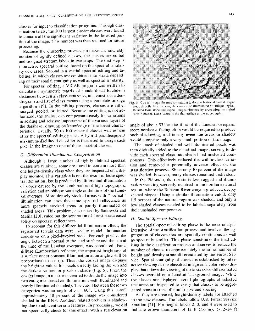
FRANKLIN e/ al.: FOREST CLASSIFICATION AND INVENTORY SYSTEM
classes for input to classification programs. Through clas-sification trials, the 200 largest cluster classes were foundto contain all the significant variation in the forested por-tion of the image. This number was thus retained for futureprocessmg.
Because the clustering process produces an unwieldynumber of tightly defined classes, the classes are editedand assigned stratum labels in two steps. The first step isinteractive spectral editing, based on the spectral similar-ity of classes. Second is a spatial-spectral editing and la-beling, in which classes are combined into strata depend-ing on their spatial contiguity as well as spectral similarity.
For spectral editing, a VICAR program was written tocalculate a symmetric matrix of standardized Euclideandistances between all class centroids, and construct a den-drogram and list of class means using a complete linkagealgorithm [19]. In the editing process, classes are eithermerged, pooled, or deleted. Because the editing is not au-tomated, the analyst can compensate easily for variationsin scaling and relative importance of the various layers ofthe database, drawing on knowledge of the forest charac-teristics. Usually, 70 to 100 spectral classes will remainafter the spectral-editing phase. A hybrid parallelepiped/maximum-likelihood classifier is then used to assign eachpixel in the image to one of these spectral classes.
G. Differential-Illumination CompensationAlthough a large number of tightly defined spectral
classes are retained, some are found to contain more thanone height-density class when they are inspected on a dis-play monitor. This variation is not the result of loose spec-tral definition, but is produced by differential illuminationof slopes caused by the combination of high topographicvariation and an oblique sun angle at the time of the Land-sat overpass. More densely stocked areas with "normal"illumination can have the same spectral reflectance asmore sparsely stocked areas in poorly illuminated orshaded areas. This problem, also noted by Sadowski andMalila [20], ruled out the separation of forest strata basedsolely on spectral reflectances.
To account for this differential-illumination effect, theregistered terrain data were used to model illuminationconditions on a pixel-by-pixel basis. For each pixel z, theangle between a normal to the land surface and the sun atthe time of the Landsat overpass, was calculated. For adiffuse (Lambertian) reflector, the apparent brightness ofa surface under constant illumination at an angle z will beproportional to cos (z). Thus, the cos (z) image displaysthe brightest values for pixels directly facing the sun andthe darkest values for pixels in shade (Fig. 5). From thecos (z) image, a mask was created to divide the image intotwo categories based on illumination: well illuminated andpoorly illuminated (shaded). The cutoff between these twocategories was an angle of z = 60°. Using this cutoff,approximately 10 percent of the image was consideredshaded in the KNF. Another, related problem is shadow-ing due to adjacent terrain features. In processing, we didnot specifically check for this effect. With a sun elevation
143
Fig. 5. Cos (z) image for area containing Eldorado National Forest. Lightareas directly face the sun; dark areas are illuminated at oblique angles.Derived from slope and aspect images obtained by processing the digitalterrain model. Lake Tahoe is the flat surface at the upper right.
angle of about 53 ° at the time of the Landsat overpass,steep northeast-facing cliffs would be required to producesuch shadowing, and in any event the areas in shadowwould comprise only a very small portion of the image.
The mask of shaded and well-illuminated pixels wasthen digitally added to the classified image, serving to di-vide each spectral class into shaded and unshaded com-ponents. This effectively reduced the within-class varia-tion and removed a potentially adverse effect on thestratification process. Since only 10 percent of the imagewas shaded, however, many classes remained undivided.
In the Eldorado, the terrain is less rugged and illumi-nation masking was only required in the northern naturalregion, where the Rubicon River canyon produced deeplyshaded slopes. Using a similar illumination cutoff, only1.5 percent of the natural region was shaded, and only afew shaded classes needed to be labeled separately fromtheir un shaded components.
H. Spatial-Spectral EditingThe spatial-spectral editing phase is the most analyst-
intensive of the stratification process and involves the ag-gregation of classes that are spatially continuous as wellas spectrally similar. This phase constitutes the final ed-iting in the classification process and serves to reduce thenumber of classes to approximately the same number ofheight and density strata differentiated by the Forest Ser-vice. Spatial contiguity of classes is established by inter-active viewing of the classified image on a color video dis-play that allows the viewing of up to six color-differentiatedclasses overlaid on a Landsat background image. Whilethe classes are displayed, aerial photographs of selectedtest areas are inspected to verify that classes to be aggre-gated contain trees of similar size and spacing.
As they are created, height-density labels are attachedto the new classes. The labels follow U.S. Forest Servicenotation [21]. For height, labels 2, 3, and 4 were used toindicate crown diameters of 12 ft (3.6 m), > 12-24 ft
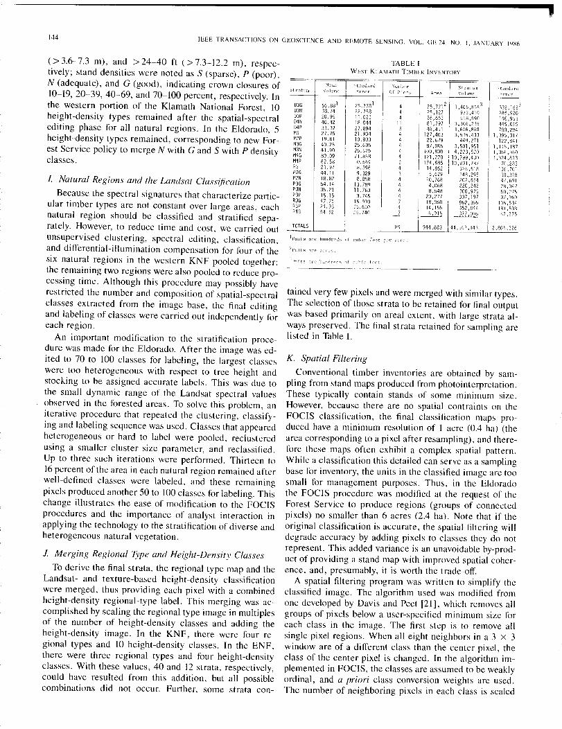
144 IEEE TRANSACTIONS ON GEOSCIENCE AND REMOTE SENSING. VOL. GE-24. NO. I. JANUARY 1986
I
J(lnits <lye hundreds c,f cuhic fpet ~Jpr acre.
(>3.6-7.3 m), and >24-40 ft (>7.3-12.2 m), respec-tively; stand densities were noted as S (sparse), P (poor),N (adequate), and G (good), indicating crown closures of10-19,20-39,40-69, and 70-100 percent, respectively. Inthe western portion of the Klamath National Forest, 10height-density types remained after the spatial-spectralediting phase for all natural regions. In the Eldorado, 5height-density types remained, corresponding to new For-est Service policy to merge N with G and S with P densityclasses.
I. Natural Regions and the Landsat ClassificationBecause the spectral signatures that characterize partic-
ular timber types are not constant over large areas, eachnatural region should be classified and stratified sepa-rately. However, to reduce time and cost, we carried outunsupervised clustering, spectral editing, classification,and differential-illumination compensation for four of thesix natural regions in the western KNF pooled together;the remaining two regions were also pooled to reduce pro-cessing time. Although this procedure may possibly haverestricted the number and composition of spatial-spectralclasses extracted from the image base, the final editingand labeling of classes were carried out independently foreach region.
An important modification to the stratification proce-dure was made for the Eldorado. After the image was ed-ited to 70 to 100 classes for labeling, the largest classeswere too heterogeneous with respect to tree height andstocking to be assigned accurate labels. This was due tothe small dynamic range of the Landsat spectral valuesobserved in the forested areas. To solve this problem, aniterative procedure that repeated the clustering, classify-ing and labeling sequence was used. Classes that appearedheterogeneous or hard to label were pooled, reclusteredusing a smaller cluster size parameter, and reclassified.Up to three such iterations were performed. Thirteen to16 percent of the area in each natural region remained afterwell-defined classes were labeled, and these remainingpixels produced another 50 to 100classes for labeling. Thischange illustrates the ease of modification to the FOCISprocedures and the importance of analyst interaction inapplying the technology to the stratification of diverse andheterogeneous natural vegetation.
J Merging Regional Type and Height-Density ClassesTo derive the final strata, the regional type map and the
Landsat - and texture-based height -density classificationwere merged, thus providing each pixel with a combinedheight-density regional-type label. This merging was ac-complished by scaling the regional type image in multiplesof the number of height-density classes and adding theheight-density image. In the KNF, there were four re-gional types and 10 height-density classes. In the ENF,there were three regional types and four height-densityclasses. With these values, 40 and 12 strata, respectively,could have resulted from this addition, but all possiblecombinations did not occur. Further, some strata con-
TABLE IWEST KLAMATH TIMBER INVENTORY
:'-lean
,ce"", ~l,r" StyntUlTl Standan:Stratum Volume Error OJ Plots l\re,~_ V0111~(' Error.... ---
03G 56.881 25.7781 4 25.7712 1,465,8553 332,16203N 38.74 ;i:6~~ I :
25,127 973,420 285,92003P 20.95 26,663 55B,590 146,95304N 40.42 18.044 II 01,797 3,306,235 445,01504P 33.37 27.894 3 48,451 1,616,810 700,284MS 27.75 21.904 4 127,403 3,535,433 1,395,317M2P I 19.81 10.833 4 22.679 449,271 122,841M3G 40.25 25.635 4 87,005 3,501,951 1,115,187M3N 41.90 26.525 4 100,800 4,223,520 1,366,360M4G 89.09 21.858 4 121,220 10,799,430 1,324,813M1P 62.58 0.569 2 174,605 10,931,787 70,283PS 21. 97 18.396 4 14,862 326,518 136,701P2G 44. II 9.329 3 5,629 248,295 30,318P2N 18.82 8.858 4 10,768 202,654 47,691P3G 54.14 13.789 4 4,068 220,242 28,047P3N
I
35.21 II. 763 4 8,54BI 300,975 50,275
P3P 15.15 3.745 4 20,277 307,197 37,%9R3G 47.75 15.900 7 18,060 862,365 lOB,S34R3P 24.93 25.650 Ji 14,155 352,844 181,538R4G 54.52 25.740 ~ ~ 67,275
TOTALS 944,883 44,561,143 2 ,BOl, 326
TTnits arE' hmdreds (1f cuhic feet.
tained very few pixels and were merged with similar types.The selection of those strata to be retained for final outputwas based primarily on areal extent, with large strata al-ways preserved. The final strata retained for sampling arelisted in Table J.
K. Spatial FilteringConventional timber inventories are obtained by sam-
pling from stand maps produced from photointerpretation.These typically contain stands of some minimum size.However, because there are no spatial contraints on theFOCIS classification, the final classification maps pro-duced have a minimum resolution of I acre (0.4 ha) (thearea corresponding to a pixel after resampling), and there-fore these maps often exhibit a complex spatial pattern.While a classification this detailed can serve as a samplingbase for inventory, the units in the classified image are toosmall for management purposes. Thus, in the Eldoradothe FOCIS procedure was modified at the request of theForest Service to produce regions (groups of connectedpixels) no smaller than 6 acres (2.4 ha). Note that if theoriginal classification is accurate, the spatial filtering willdegrade accuracy by adding pixels to classes they do notrepresent. This added variance is an unavoidable by-prod-uct of providing a stand map with improved spatial coher-ence, and, presumably, it is worth the trade-off.
A spatial filtering program was written to simplify theclassified image. The algorithm used was modified fromone developed by Davis and Peet [21], which removes allgroups of pixels below a user-specified minimum size foreach class in the image. The first step is to remove allsingle pixel regions. When all eight neighbors in a 3 x 3window are of a different class than the center pixel, theclass of the center pixel is changed. In the algorithm im-plemented in FOCIS, the classes are assumed to be weaklyordinal, and a priori class conversion weights are used.The number of neighboring pixels in each class is scaled
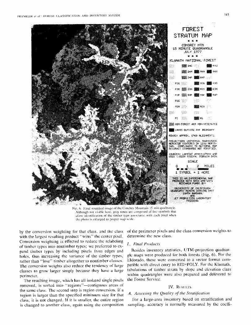
FRANKLIN C{ III.: FOREST CLASSIFICATION AND INVENTORY SYSTEM
FDRESTSTRATUM MAP
)II )II 1«
CONDREY MTNMINUTE QUADRANGLE·JULl' 1977
)ll lIi III
KLAMATH NATIONAL FORESTIIIID4G .R4C;
II D4M .11411 • fi'4l'1
l1li D4f' • M4P
PSG • 11313 • R3G
f'3tl l1li D3t1 • M3N • R3H
P3P D3P • M3P.1<31'
PeG.MZN
• tiS
NON-fOREST AND NON-VEGETATED
Fig. 6. Final stratified image of the Condrey Mountain 15-min quadrangle.Although not visible here, gray tones are composed of fine symbols thatallow identification of the timber type associated with each pixel whenthe photo is enlarged to proper map scale.
145
by the conversion weighting for that class, and the classwith the largest resulting product "wins" the center pixeLConversion weighting is effected to reduce the relabelingof timber types into nontimber types; we preferred to ex-pand timber types by including pixels from edges andholes, thus increasing the variance of the timber types,rather than "lose" timber altogether to nontimber classes.The conversion weights also reduce the tendency of largeclasses to grow larger simply because they have a largeperimeter.
The resulting image, which has all isolated single pixelsremoved, is sorted into "regions"-contiguous areas ofthe same class, The second step is region conversion. If aregion is larger than the specified minimum size for thatclass, it is not changed. If it is smaller, the entire regionis changed to another class, again using the composition
of the perimeter pixels and the class conversion weights todetermine the new class.
L Final ProductsBesides inventory statistics, UTM-projection quadran-
gle maps were produced for both forests (Fig, 6), For theEldorado, these were converted to a vector format com-patible with direct entry to RID*POLY. For the Klamath,tabulations of timber strata by slope and elevation classwithin quadrangles were also prepared and delivered tothe Forest Service.
IV. RESULTS
A. Assessing the Quality of the StratificationFor a large-area inventory based on stratification and
sampling, accuracy is normally measured by the coeffi-
------------------------------liliiii1146 IEEE TRANSACTIONS ON GEOSCIEt\CE AND REMOTE SENSIt\G. VOL. GE-24. NO. I. JANLARY 19X6
cient of variation of the estimated quantity-the lower thestandard error of the estimate with regard to the mean, themore accurate is the inventory. Since the Klamath and El-dorado inventories included ground samples of timber vol-ume, it was possible to estimate this standard error in bothcases. For the Klamath, however, a concurrent timber in-ventory carried out by the Forest Service using conven-tional techniques was also available. In the case of the El-dorado, a full and complete Landsat-based inventory wasthe objective. Thus, no concurrent alternative inventorywas available for comparison there. The remaining sec-tions in this portion of the paper document sample allo-cation, data collection, and calculation of totals and stan-dard errors.
B. Field Data Collection
Following definition of the final strata, the actual per-acre timber volume associated with each stratum must beestimated. These estimates are obtained from groundsamples, or "cluster plots," collected according to stan-dardized procedures specified by Region 5 of the USFS[21]. These ground samples are termed cluster plots be-cause each consists of five subplots clustered in the shapeof an "L," with one subplot at the vertex and two alongeach arm. The arms of the cluster plot are oriented duenorth and due east with the subplots located two chains(132 ft, 40.2 m) apart. The use of such spatially clusteredsamples is a classic sampling technique that is invokedwhen local variance is high and the travel cost to reachrandomly located points is excessive [23]. In the case ofthe Eldorado, the distance between subplots was adjustedto 100 ft (30.5 m), or about half the interpixel ground dis-tance, to avoid interaction between the cluster plot layoutand the pixel grid.
The cluster plot data collected at the individual pointsincluded height, diameter at breast height (DBH), andgrowth increment for a systematically selected subsampleof trees; and height and DBH class, damage and defectcodes, and other information for all remaining trees fail-ing within variable-radius plots defined using standardwedge prism methods [21 J. In the processing of the plotsby the Forest Service, variables are averaged over all thesubplots and weighted by the number of subplots withinthe plot for which it was actually possible to collect data.Degrees of freedom in inventory calculations, however,are determined by the number of plots, not subplots. Thisprocedure results in a conservative estimate of within-stratum variance.
C. Sample Allocation
Estimating the average timber volume for each Landsat-derived stratum requires allocating cluster-plot samples toeach stratum. A random stratified sample design withequal numbers of samples for each stratum is consideredappropriate by the Forest Service for this purpose. A min-imum of four cluster plots per stratum is the rule of thumbused for Region 5 forests; this criterion implies 68 clusterplot samples for the Landsat-based strata in the KNF. Un-
fortunately, funds were not available to collect this largenumber of cluster plots independently, and it became nec-essary to rely in part on the cluster plots collected by theForest Service for their forest-wide inventory. This plot-sharing procedure added an unknown bias to the FOCIStimber-volume total, but it was unlikely to affect the stan-dard error of the estimate [21.
Another problem in sample allocation in the Klamathinventory arose because of a Forest Service decision tomerge strata with similar stocking densities, thus creatinga smaller number of strata than originally planned. In ad-dition, since the new strata were expected to be somewhatmore variable than the older ones, the intensity of ForestService sampling by the Forest Service was increased,with at least six cluster samples obtained for each stratum.Thus, the final strata used by the USFS and produced byFOCIS did not correspond exactly for the KNF.
Neither of these problems arose in the Eldorado inven-tory, since all samples were allocated according to the FO-CIS stratification. Fifty-six plots were allocated in theeight FOCIS timber strata, and after collection, the datawere processed by Forest Service software to derive tim-ber volume estimates.
D. Landsat-Based Timber Volume Inventory
In order to assess the accuracy of the inventories, wefocused on one inventory statistic-total softwood timbervolume f{)r the forest-obtained by areal weighting ofwithin-stratum volume averages. Areas of strata were eas-ily obtained from tabulations of pixels; mean and varianceof softwood volume were derived from the processing ofthe cluster plots.
Table I presents the inventory total and its standard errorfor the western region of the KNF. For the mapped areasof 944 833 acres (422 340 ha), the value is 3.83 X 10⁹
ft3 (1.08 X 10⁸ m3), with a standard error of 0.187 X 10⁹
ft3 (0.053 X 10⁸ m3). This standard error represents 4.88percent of the total timber volume. In comparison, theForest Service inventory yielded a timber total of 2.69 X109 ft3 (0.76 X 10⁸ m3), with a standard error of 0.067 X109 ft3 (0.019 X 10⁸ m3) for an area of I 082 000 acres(438 000 ha) [2]. This error is about 2.5 percent of thetotal.
A comparison of the two inventories shows that eachyielded significantly different timber-volume totals-theFOCIS volume was about 40 percent larger than that es-timated by the Forest Service. However, the higher valuefor the FOCIS inventory results largely from high meanvalues for the two M4 strata. Although four Forest Serviceplots were allocated to M4P, data f{)r only two of the plotswere received. Also note that the standard error of theM4P FOCIS stratum is very low-0.569 X 102 ft3 (1.61m3 )-compared to the rest of the values, which rangeroughly from 5 to 25. This value is probably accidental,resulting because the two plots were, by chance, very closein timber volume. This low standard error, multiplied bythe large area of the stratum, reduces the standard errorof the total significantly, making it look better than it really

FRANKLIN el al.: FOREST CLASSIFICATION AND INVENTORY SYSTEYl
TABLE IIELDORADO TI\1BFR 1NVENTORY
~lean Stanc.ard Numbt', Stratum St:wdardStratum Vo 1ume Errelr Of Plcts Area Volume I~rrcr
~13(; 56.8511 8. JOOI8 78, <")322 4,464.62J3 :':3C, /"::;63
:-13P 42.759 15.14R 8 122,400 5,233.702 ,62b
~14G 74.015 10.255 8 ".1,409 3 ,809 ,478 I ,(-)]9
\141' 54.071 10.364 8 43,579 2,356,360 1 'i 'J, 70'7
R3G 86.634 23.310 6 10,701 927,070 101,
R3P 30.936 6.722 6 12,288 380,142 J 3,728
R4G 9] .536 24.427 6 10,493 960,487 104, h 60
R4P 51. 419 11. 205 ~ 13,356 686,752 61, 100
Totals 56 342,818 1R,81S,614 7 5 ~, 545
lUnits are hundreds of cuhic feet per acre.
2Untts are acres.
3Units are hundreds cf c111~ic :eet.
147
is. If the means and variances for M4P and M4G obtainedin the Forest Service inventory are substituted for thoseobtained by the FOCIS procedure, the FOCIS total dropsto 2.87 x 109 ft3 (0.81 X 10⁸ m3), with a standard errorof 0.161 X 109 ft3 (0.046 X 10⁸ m3). This adjustmentbrings the two timber volume totals to within approxi-mately one and one-quarter standard errors of each other.
Note also that these modifications raise the FOCIS stan-dard error to 5.61 percent of the total timber volume. Thisaccuracy value, approximately 6 percent, probably betterrepresents the true value achieved using the Landsat-basedmethodology of FOCIS. Compared to the value of 2.51percent of the Forest Service inventory, it is more thantwice as large. However, that the standard errors are notdirectly comparable, since the total areas of the two in-ventories are different and each is based on a differentnumber of samples chosen from a different number ofstrata. By expressing the timber volume on a per-acre ba-sis, and by correcting for degrees of freedom in sampling,the per-acre per-sample standard errors are 0.573 and0.332 ft3 (0.0162 and 0.0094 m3), respectively, for FOCISand Forest Service inventories. In this comparison, theFOCIS value is higher than that of the Forest Service, butis still well within the 7.5-percent USFS guideline.
Table II presents inventory statistics for the EldoradoNational Forest. The inventory showed a total softwoodvolume of 1.88 X 10⁹ fe (0.53 x 10⁸ m3) for an area of342 818 acres (138 738 ha). The standard error of the tim-ber volume estimate was 0.075 X 109 ft3 (0.021 X 10⁸
m3), representing almost exactly 4.0 percent of the mean.This value compares favorably with that obtained in theKlamath, and is also well within Forest Service guide-lines.
In the Eldorado, the accuracy of the stratification label-ing for all strata, including nonforest types, was also as-sessed. Table III presents a crosstabulation of predictedand actual labels for a set of points randomly selected toverify accuracy. Of the 128 points, 108 were correctly la-beled, yielding an overall accuracy of 84.4 percent. Thetable does not reveal that any strata were consistently mis-
labeled; at least five of the eight points were correct forall strata, and 10 of the 16 strata showed seven or eightcorrect points. The overall accuracy compares favorablywith the highest values heretofore reported [11] and isclose to the 90-percent level, which is occasionallyachieved in Level I classification of Landsat MSS imagery[24]. Because many of our classes correspond to Level IIIclasses, our accuracy probably represents the maximumattainable in a realistic situation. Using the binomial dis-tribution, it is possible to place confidence intervals on theaccuracy; a 5-percent confidence interval ranges from 76.6to 89.8 percent [25].
An alternative method for evaluating a confusion tablewas suggested by Card [26] in which the marginal totalsof the table and the area of each stratum are used to pro-vide an overall accuracy and confidence interval, as wellas estimates of the true area for each stratum and associ-ated confidence intervals. The overall accuracy calculatedby this method improved to 87.0 percent, but the confi-dence interval widened to 79.5 to 94.4 percent, indicatingthat there is no significant difference between the two ac-curacy estimates. Using the new estimate of the area foreach stratum, the timber inventory statistics can be recal-culated. The total timber volume estimate increased by 3.7percent and the standard error of this new estimate wasreduced to 3.5 percent.
V. CONCLUSION
The FOCIS procedure for timber volume inventory usingLandsat MSS, texture and digital terrain information wasdeveloped, tested and refined over a 6-year period in twolarge forests in California. By incorporating the same ele-ments of tone, texture, and terrain used in manual delin-eation of forest stands, FOCIS can produce a softwoodtimber volume estimate for very large areas with a stan-dard error comparable to estimates produced by conven-tional means. Because part of the FOCIS procedure is au-tomated and based on Landsat technology, the per-acrecost of timber inventory should be significantly lower thanthat of conventional methodologies. Further, FOCIS meth-
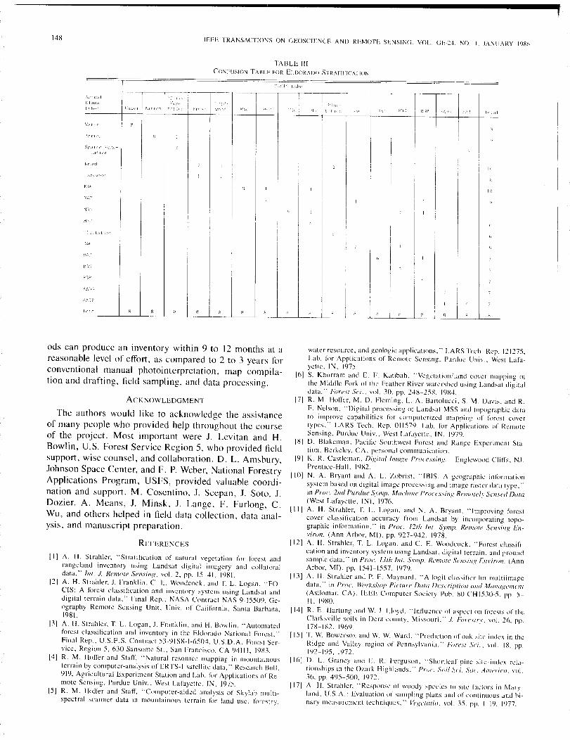
------------------------------~,148 IEEE TRA1\SACTlONS ON GEOSCIENCE ANO REMOTE SENSING. VOL GE-24. 1\0 I. JANUARY 1986
TABLE 1IlCOI\FlISION TABLE FOR ELDORADO STRATIFICATION
::las.-.;Labei
1'.1'Tf'll
Spar(l>t;itl()1l
hru~;l
--l",,:-::.-r-]\;lrr":l rat iCIl ! l'rllc;!l
1"l:J1
M'jl'
1'1 iirttilt
JU,(
S,"dP
rctnl
In
ods can produce an inventory within 9 to 12 months at areasonable level of effort, as compared to 2 to 3 years forconventional manual photointerpretation, map compila-tion and drafting, field sampling, and data processing.
ACKNOWLEDGMENT
The authors would like to acknowledge the assistanceof many people who provided help throughout the courseof the project. Most important were J. Levitan and H.Bowlin, U.S. Forest Service Region 5, who provided fieldsupport, wise counsel, and collaboration. D. L. Amsbury,Johnson Space Center, and F. P. Weber, National ForestryApplications Program, USFS, provided valuable coordi-nation and support. M. Cosentino, J. Scepan, 1. Soto, 1.Dozier, A. Means, 1. Minsk, J. Lange, F. Furlong, C.Wu, and others helped in field data collection, data anal-ysis, and manuscript preparation.
REFERENCES
[I] A. H. Strahler, '"Slratifieation of natural vegetation f(Jr forest andrangeland inventory using Landsat digital imagery and collateraldata," 1m. 1. Remole Sensing, vol. 2. pp. 15-41, 1981.
[2] A. H. Strahler. J. Franklin. C. E. Woodcock, and 1'. L. Logan, '"FO-CIS: A I(Jrest classification and inventory system using Landsat anddigital terrain data." Final Rep .• NASA Contract NAS-9-15509, Ge-ography Remote Sensing Unit. Univ. of Calil(Jrnia, Santa Barbara.1981.
[3J A. H. Strabler. 1'. L. Logan. J. Franklin. and H. Bowlin, '"Automatedforest classification and inventory in the Eldorado ",ational Forest.·'Final Rep .. U.S.F.S. Contract 53-9IS8-1-6504, U.S.D.A. Forest Ser-vice, Region 5, 630 San some SI., San Francisco. CA 94111,1983.
[41 R. M. HolIer and StafL "Natural resource mapping in mountainousterrain by computer-analysis of ERTS-I satell ite data," Rcsearch Bull.919, Agricultural Experiment Station and Lab. for Applications of Re-mote Sensing, Purdue Univ., West Lafayette, IN, 1975.
15] R. M. Hoffer and Staff, '"Computer-aided analysis of Skylab multi-spectral scanner data in mountainous terrain for land use. I(lrestry,
water resource, and geologic applications," LARS Tech Rep. 121275,Lab. I(Jr Applications of Remote Sensing. Purduc Univ., West Lafa-yette, IN, 1975.
16J S. Khorram and E. F. Katibah, '"Vegetation/land cover mapping ofthe Middle Fork of the Feather River watershed using Landsat digitaldata," f(m'sl Sci .. vol. 30, pp. 248-258, 1984.
17] R. M. Hoffer, M. D. Fleming, L. A. Bartolucci, S M. Davis, and R.F. Nelson, '"Digital processing of Landsat MSS and topographic datato improve capabilities I(,r computerized mapping of I(lrest covertypes," LARS Tech. Rcp. 011579, Lab. 1(". Applications of RemoteSensing, Purdue Univ., West Lafayettc, IN, 1979.
181 D. Blakeman. Pacific Southwest Forest and Range Experiment Sta-tion, Berkcley, CA, personal communication.
19] K. R. Castleman, Digilallmage Processing. Englewood Cliffs, NJ:Prentice-Hall. 1982.
IIOJ N. A. Bryant and A. L. Zobrist. '"IBIS: A geographic int()rmationsystem based on digital image processing anu image raster uata type,"in Proc. 2nd Purdue S\'ml'. Machille Processillg Rell/ole!." Sell.\ed DIIIII(West Lafayette, [N), 1976.
[1[1 A. H. Strahler, 1'. L. Logan, and N. A. Bryant, "Improving f(Jrestcover elassilication accuracy from Landsat by incorporating (opo-graphic inf(mnation," in Proc. 12/h Inl. SYlI/p. RemOie Sensing En-vimll. (Ann Arbor, M[), pp. 927-942, 1978.
II2J A. H. Strahler, T. L. Logan, and C. E. Woodcock. "Forest classifi-cation and inventory system using Landsat, digital terrain, and groundsample data," in Proc. /3/h 1111. SYlI/p. RCII/ole Sensil/g FI/I'iron. (AnnArbor, MI), pp. 1541-1557, 1979.
[13] A. H. Strahler and P. F. Maynard, "A logit classifier I(lr multiimagedata." in Proc. Worksho!, Pic/un' Dmll Descriplion and Mal/agell/enl(Asilomar, CA), IEEE Computer Society Pub. 80 CH 1530-5, pp. 5-II. 1980.
114J R. E. Hartung and W. J. Lloyd, "Influence of aspect on forests of theClarksville soils in Dent county, Missouri," .I. I'i,reslrv, vo!. 26, pp.178-182, 1969.
1151 1'. W. Bowersox and W. W. Ward, "Prediction of oak site index in theRidge and Valley region of Pennsylvania," f(,res/ S<'i., vol. 18, pp.192-195, 1972.
1161 D. L. (-,raney and E. R. Ferguson, "Sllllrtleaf pine site-index rela-tionships in the Ozark Highlands," Proc. Soil Sci. Soc All/aim, vo!.36, pp. 495-500, 1972.
[171 A. H. Strahler, "Response of woody specics to site factors in Mary-land. U.S.A.: Evaluation of sampling plans and of continuous and bi-nary measurement techniques." Vege/alio, vo!. 35. pp. 1-19. 1977.
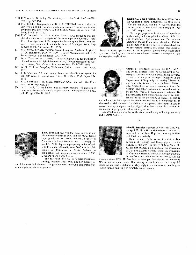
*
FRANKLIN et al. FOREST CLASSIFICATION AND INVENTORY SYSTEM
118] R. Tryon and D. Bailey, Cluster Analysis. New York: McGraw-Hili,1970, pp. 147-150.
[191 F. J. Rohlf, J. Kishpaugh. and D. Kirk, "NT-SYS: Numerical taxon-omy system of multivariate statistical programs." documentation andprograms available from F. J. Rohlf, State University of New York.Stony Brook, NY, 1974.
[20J F. G. Sadowski and W. A. Malila, "Reflectance modeling and em-pirical multispectral analysis of forest canopy components," FinalRep., Investigations of Techniques t(lr Inventorying Forest Regions,vol. I, Environmental Research Institute of Michigan Tech. Rep.122700-35-F I. Ann Arbor, ML 1977.
[21] U.S. Forcst Service, "Compartment Inventory Analysis: Region 5C.I.A. Handbook, Mar. 19, 1979." Timber Management Staff, U.S.Forest Service, San Francisco. CA, 1979.
122] W. A. Davis and F. G. Peet, "The identification and reclassificationof small regions in digital thematic maps," Forest Management Insti-tute, Ottawa. Ont., Canada, Int()rmation Rep. FMR ..X-90, 1976.
[231 W. G. Cochran, Sampling Techniques, 3rd ed. New York: Wiley,1977.
[24] J. R. Anderson, "A land use and land cover classification system foruse with remotely sensed data," US. Ceo. Surv. Prof Paper 964,1976.
[25] F. J. Rohlf and R. R. Sokal, Statistical Nihles, 2nd ed. San Fran-cisco: W. H. Freeman, 1981.
[261 D. H. Card, "Using known map category marginal frequencies toimprove estimates of thematic map accuracy," Photogrammetr. Eng.,vol. 48, pp. 431-439, 1982.
*
Janet Franklin received the B.A. degree in en-vironmental biology in 1979 and the M.A. degreein geography in 1983. both from the University ofCalif(lrnia at Santa Barbara. She is working to-ward the Ph. D. degree in geography under a Grad-uate Research Fellowship from NASA at the Uni-versity of Calij(lrnia at Santa Barbara inconjunction with ongoing research at the NASAGoddard Spacc Flight Center.
She has been involved in vegetation/remote-sensing research since 1978, and her current re-
search interests include forest canopy reflectance modeling, and spatial pat-tern analysis in natural vegetation.
149
Thomas L. Logan received the B.A. degree fromthe Calit()rnia State University. Northridge, in1976 and the M.A. and Ph.D. degrees from theUniversity of California at Santa Barbara in 1978and 1983, respectively.
He is a geographer with ]() years of experiencein the Cartographic Applications Group of the Im-age Processing Applications and DevelopmentSection at the Jet Propulsion Laboratory, Califor-nia Institute of Technology. His emphasis has beenon the remote sensing and image processing of
forest and range applications, as well as general geographical informationsystems technology, classification techniques, database development, andcartographic applications.
Curtis E. Woodeoek received the B.A., M.A.,and Ph.D. degrees from the Department of Ge-ography, University of Calitornia, Santa Barbara.
He is currently an Assistant Professor in theDepartment of Geography and Acting Director ofthe Center t()r Remote Sensing at Boston Univer-sity. Applications of remote sensing to torest in-ventory and other problems in natural environ-ments have been a primary research interest. Hehas conducted both empirical and theoretical stud-ies on the spatial properties of images, assessing
the influence of both spatial resolution and the nature of environments onobserved spatial patterns. The ability to incorporate other types of data inremote sensing analyses, such as digital elevation models. has resulted inan interest in geographic information systems.
Dr. Woodcock is a member of the American Society of Photogrammetryand Remote Sensing.
*Alan H. Strahler was born in New York City, NY,on April 27, 1943. He received the B.A. and Ph.D.degrees from the Johns Hopkins University in 1964and 1969, respectively.
He is currently Professor and Chair of the De-partment of Geology and Geography at HunterCollege of the City University of New York. Hehas held prior academic positions at the Universityof Calilornia, Santa Barbara, and at the Universityof Virginia. Originally trained as a biogeographer,he has been actively involved in remote-sensing
research since 1978. He has been a Principal Investigator on numerousNASA contracts and grants. His primary research interests are in spatialmodeling and spatial statistics as they apply to remote sensing, and in geo-metric-optical modeling of remotely sensed scenes.
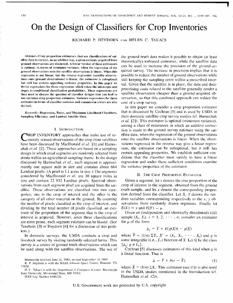
150 IEEE TRANSACTIONS 01'; GEOSCIENCE AND REMOTE SENSING. VOL. GE-24. NO. I. JANUARY 1986
On the Design of Classifiers for Crop InventoriesRICHARD P. HEYDORN AND HELEN C. TAKACS
I
Abstract-Crop proportion estimators that use classifications of sat-ellite data to correct, in an additive way, a given estimate acquired fromground observations are discussed. A linear version of these estimatorsis optimal, in terms of minimum variance, when the regression of theground observations onto the satellite observations is linear. When thisregression is not linear, but the reverse regression (satellite observa-tions onto ground observations) is linear, the estimator is suboptimalbut still has certain appealing variance properties. In this paper wederive expressions for those regressions which relate the intercepts andslopes to conditional classification probabilities. These expressions arethen used to discuss the question of classifier designs that can lead tolow-variance crop proportion estimates. Variance expressions for theseestimates in terms of classifier omission and commission errors are alsoderived.
Keywords-Regression, Bayes, and Maximum Likelihood Classifiers,Sampling Efficiency, and Landsat Satellite Data.
I. INTRODUCTION
CROP INVENTORY approaches that make use of re-motely sensed observations of the crop from satellites
have been discussed by MacDonald et at. [I] and Hanus-chak et at. [2]. These approaches are based on a samplingdesign in which areal segments are randomly selected fromstrata within an agricultural sampling frame. In the designdiscussed by Hanuschak et at., each segment is approxi-mately one square mile in size and contains about 664Landsat pixels. (A pixel is l.l acres in size.) The segmentsconsidered by MacDonald et at. are 30 square miles insize and contain 22 932 Landsat pixels. Spectral obser-vations from each segment pixel are acquired from the sat-ellite. These observations are classified into two cate-gories; one is the crop of interest and the other is thecategory of all other material on the ground. By countingthe number of pixels classified as the crop of interest, anddividing by the total number of pixels classified. an esti-mate of the proportion of the segment that is the crop ofinterest is acquired. However, since these classificationsare error prone, each segment estimate can be biased. (SeeTenebein [31 or Heydorn [41 for a discussion of this prob-lem.)
In domestic surveys, the USDA conducts a crop andlivestock survey by visiting randomly selected farms. Thissurvey is a source of ground truth observations which canbe used along with the satellite observations. The use of
the ground truth data makes it possible to obtain (at leasttheoretically) unbiased estimates, while the satellite datacan be used to increase the precision of the ground-ac-quired survey. The increase in precision implies that it ispossible to reduce the number of ground observations whilestill keeping the sampling error within a prescribed inter-val. Given that the satellite is in place, the data and data-processing costs related to the satellite generally render asatellite observation cheaper than a ground-acquired ob-servation, so that this combined approach can reduce thecost of a crop survey.
In this paper we consider a crop proportion estimatorthat is discussed by Cochran [51 and is used by USDA intheir domestic satellite crop survey studies (cf. Hanuschaket at. [2]). This estimator is optimal (minimum variance),among a class of estimators in which an additive correc-tion is made to the ground survey estimate using the sat-ellite data, when the regression of the ground observationsonto the satellite observations is Iinear. When the obser-vations regressed in the reverse way give a linear regres-sion, the estimator can be suboptimal, but it still hascertain appealing properties. We establish sufficient con-ditions that the classifier must satisfy to have a linearregression and under these sufficient conditions examinethe variance properties of the estimator.
II. THE CROP PROPORTIONESTIMATOR
Given a segment, let y denote the true proportion of thecrop of interest in the segment, obtained from the groundtruth sample, and let x denote the corresponding propor-tion derived from the classifier. Let X, Y denote the ran-dom variables corresponding respectively to the x, y ob-servations from randomly drawn segments. Finally letE(X) = rand E(Y) = 11.
Given an (independent and identically distributed) (iid)sample (Xi' Yi), i I, 2, ... , n, consider an estimatorfor 11 of the form
I1g Y + E(g(K)) - g(K)
where Y = (1/n) EYi, K' = (XI' X2, •••• X,,) and g issome integrable (i.e., Lj) function ofK Let g be the class{P,g: gELd·
Cochran [5] discusses estimators of this kind when g isa linear function. That is
where X = (1In) EXi. This estimator (see (1)) is also usedin the USDA studies mentioned in the Introduction (cf.Hanuschak et at. (2)).
Manuscript received June 12. ]985; revised September 10. 1985.R. P. Heydorn is with the NASA Johnson Space Center. Houston. TX
77058.H. C. Takacs is with the Department of Computer Science. Mississippi
State University. Mississippi State. MS 39762.IEEE Log Number 8406226.
p, = Y + her - X) (I)
U.S. Government work not protected by U.S. copyright

HEYDORN AND TAKACS: DESIGN OF CLASSIFIERS FOR CROP INVENTORIES 151
Both /1,g and /1, are clearly unbiased and since
Var (/1,g) = E(Var (/1,gIK» + Var (E(/1,gIK»
= E(Var (PIX» + Var (E(PIX) - g(K». (2)
/1,g will have minimum variance (and therefore minimummean square error sinc~ E(/1,g) = J-t) among the membersof class g if g(K) = E(YIK) + c where c is any constant.
The last term in (2) measures the increase in variancewhen failing to match (within a constant) the true regres-sion function when selecting g. In particular the linear ver-sion in (1) may be suboptimal, but since b is the only pa-rameter that needs to be estimated, it is an appealingchoice. We are assuming that the satellite provides us witha large number of observations, and therefore, v can becomputed (i. e., estimated with virtually zero variance).This is the case in the above-mentioned USDA studies.
For the estimator of (1)
(5)
(4)E(Eel1>:.(Z), ~) = 0
1>:.(Z) = {31:' + (32:.8 + EI'>'
E(Eq,18, ~) = 0
where
aIX = E(811):.(Z) = 0, X)an = E(811):.(Z) = 1, X) - a,x(31Y = E(1):.(Z)18 = 0, Y)(32Y = E(1):.(Z)18 = 1, Y) - (3,y.
al:' = E(811):.(Z) = 0, ~),
a2:' = E(811):.(Z) = 1, ~) - al:'
{3,:. = E(1):.(Z)18 = 0, M,
(32:' = E(1):.(Z)1 8 = 1, ~) - (3,:..
Y = E(81~).
We will be interested in the regression functions E(YIX)and E(X 1 Y) and to study these functions we will start withsimple "two-point-models"
8 = al:' + a2:.1>:.(Z) + Ee,
and
Theorem(i) E(YIX) = alX + a2XX(ii) E(X I Y) = {3, Y + (32YY
which, as we will show in the next theorem, have the ca-pability of generating our regression functions. Notice thatsince 8 and 1>:.(Z) can only assume two values, the con-ditional expectations of the errors are zero when we makeproper choices for the a's and the (3's. Clearly, thesechoices should be
servation on the crop of interest when we write 1>(z) = 1and on some other material when we write 1>(z) = O. Fi-nally we let ~ be a random variable that indexes the seg-ments in the sample.
In the development to follow we will allow for the optionto alter the classifier depending upon some property of thesegment being classified, i.e., the classifier can be a func-tional of ~. We denote this fact by writing 1>!',.
Given the early definition of X and Y along with theabove definitions, we see that
A proof of this theorem is given in the Appendix.We saw in the previous section that /1, of (1) is optimal
among members of class g when E(YIX) is linear. Thetheorem shows that this regression function will be linearif (but not only if) a,x and a2X are constants. The func-tions a,x and a2X are made up of conditional expectations(or conditional probabilities since 8 assumes only 0 or 1)where the conditioning depends on the classifier 1>:.. If wefix X, at say X = x, then x could be treated as a parameter;and further, if 1>:. were a function of 8, rather than z, the
(3)+ (b _ cov (X, y»)2 Var (X)Var (X) n
2 Var (Y)Var (/1) = (1 - R ) --
n
where R = cov (X, Y)/.JVar (X) Var (Y). The best choicefor b is cov (X, Y)/Var (X) regardless of the form of theregression function. The term 1 - R2 i~ the variance re-duction afforded by using /1, in place of Y as an estimatorfor J-t.
If E(XIX) were linear (where X' = (Y), Y2, ... , YIl»,then the minimum mean square erro!:.JMSE) estimator forv among estimators of the form vf = X + E(.f(X» - f(X),fELl' would have a variance reduction that is again 1 -R2
• Hence, /1, will estimate J-t at least as well (in terms ofR2) as vf can estimate v when E(X IX) is linear.
Based on these considerations related to the estimatorof (1), we next consider some possible properties of theclassifier that can lead to Iinear regression models.
III. THE CLASSIFIER AND REGRESSIONS
To introduce some of the ideas in this section, we willneed the following notation.
Let Z be the random variable of satellite pixel observa-tions z. Since the satellite is capable of acquiring datawithin several spectral wavelengths (Landsats I through 3acquire data within four wavelength ranges and Landsat 4within up to seven) and views the same spot on the Earthmultiple times during a year, Z is generally a vector ratherthan a scalor. Let 8 be the random variable that denotesthe label of an observed pixel. When 8 assumes a value of1, the pixel being observed is the crop of interest, andwhen 8 assumes the value of 0, the pixel is some othermaterial. The satellite provides us only with values of Z.Values of 8 must be obtained by other means, such as fromground observations. The purpose of the classifier will beto use Z to estimate 8. We denote the classifier by thefunction 1> where 1>(z) E {O, I}. We classify z as an ob-
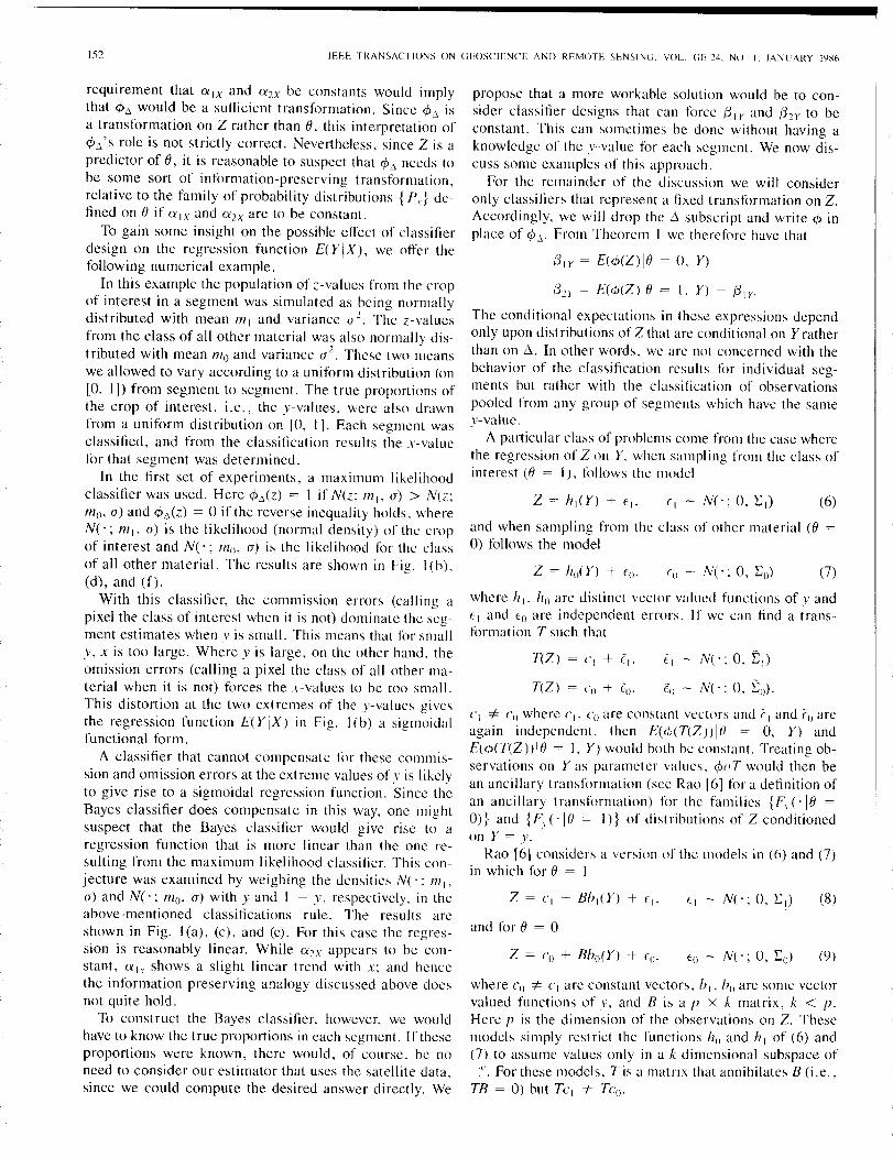
152 IEEE TRANSACTIONS ON GEOSCIENCE AND REMOTE SENSING, VOL. c;F~4, NO, I. JANUARY 1986
(8)
(6)
(7)
(9)
N('; O. tl)
N(' : 0, to).
EO - N('; 0, LO)Z = ho(Y) + Eo.
T(Z) = Co + Eo,
Z = ('I + Bbl(Y) + (I.
and for e = 0
and when sampling from the class of other materia] (0 =
0) follows the model
propose that a more workable solution would be to con-sider classifier designs that can force {31rand {3n to beconstant. This can sometimes be done without having aknowledge of the y-value for each segment. We now dis-cuss some examples of this approach.
For the remainder of the discussion we will consideronly classifiers that represent a fixed transformation on Z.Accordingly, we will drop the Li subscript and write <1>inplace of <1>t:..From Theorem I we therefore have that
{3IY = £(<1>(Z)IO = o. Y)
{3n = £(<1>(Z)IO = I, Y) - {3IY'
The conditional expectations in these expressions dependonly upon distributions of Z that are conditional on Y ratherthan on Li. In other words, we are not concerned with thebehavior of the classification results fClr individual seg-ments but rather with the classification of observationspooled from any group of segments which have the samey-value.
A particular class of problems come from the case wherethe regression of Z on Y. when sampling from the class ofinterest (0 = I). Ic)lIows the model
where Co "* CI are constant vectors, hi, bo are some vectorvalued functions of y. and B is a p X k matrix, k < p.Here p is the dimension of the observations on Z. Thesemodels simply restrict the functions ho and hi of (6) and(7) to assume values only in a k dimensional subspace of
p. For these models. T is a matrix that annihilates B (i.e.,TB = 0) but TCI "* Tc().
where hi. ho are distinct vector valued functions of y and(I and (0 are independent errors. II' we can find a trans-formation T such that
CI "* Co where CI, Co are constant vectors and E I and Eo areagain independent, then £(<1>( T(Z)) 1 () = O. Y) andE(<1>(T(Z))IO = I, Y) would both be constant. Treating ob-servations on Yas parameter values, <1>oT would then bean ancillary transformation (see Rao [61 for a definition ofan ancillary transformation) f(lr the famil ies {F, (-I e =O)} and {F,('le = I)} of distributions of Z conditionedon Y = y.
Rao [61 considers a version of the models in (6) and (7)in which for e = I
requirement that a IX and a2X be constants would implythat <1>t; would be a sufficient transformation. Since <1>t; isa transformation on Z rather than 0, this interpretation of<1>t;'S role is not strictly correct. Nevertheless, since Z is apredictor of 0, it is reasonable to suspect that <1>t; needs tobe some sort of information-preserving transformation,relative to the family of probability distributions { P,} de-fined on 0 if a IX and an are to be constant.
To gain some insight on the possible effect of classifierdesign on the regression function £( Y I X), we offer thefollowing numerical example.
In this example the population of z-values from the cropof interest in a segment was simulated as being normallydistributed with mean Inl and variance a~. The z-valuesfrom the class of all other material was also normally dis-tributed with mean Ino and variance a~. These two meanswe allowed to vary according to a uniform distribution (on[0, I]) from segment to segment. The true proportions ofthe crop of interest, i.e., the y-values, were also drawnfrom a uniform distribution on [0, 1]. Each segment wasclassified, and from the classification results the x-valuefor that segment was determined.
In the first set of experiments, a maximum likelihoodclassifier was used. Here <1>t:.(z) = I if N(z; f111, a) > N(z;!n(h a) and <1>t:.(z) = 0 if the reverse inequality holds, whereN('; !nl, a) is the likelihood (normal density) of the cropof interest and N('; !n(), a) is the likelihood f()f the classof al] other material. The results are shown in Fig. ](b).(d), and (f).
With this classifier, the commission errors (calling apixel the class of interest when it is not) dominate the seg-ment estimates when y is small. This means that for smally, x is too large. Where y is large, on the other hand, theomission errors (calling a pixel the class of all other ma-teria] when it is not) forces the x-values to be too small.This distortion at the two extremes of the y-values givesthe regression function £( Y I X) in Fig. I (b) a sigmoidalfunctional form.
A classifier that cannot compensate for these commis-sion and omission errors at the extreme values of y is likelyto give rise to a sigmoidal regression function. Since theBayes classifier does compensate in this way, one mightsuspect that the Bayes classifier would give rise to aregression function that is more Iinear than the onc re-suIting from the maximum likelihood classifier. This con-jecture was examined by weighing the densities N('; !nl,a) and N('; !n(), a) with yand I - y, respectively. in theabove-mentioned classifications rule. The results areshown in Fig. I (a). (c), and (e). For this case the regres-sion is reasonably linear. While a~x appears to be con-stant, air shows a slight linear trend with x; and hencethe information preserving analogy discussed above doesnot quite hold.
To construct the Bayes classifier. however. we wouldhave to know the true proportions in each segment. If theseproportions were known, there would, of course. be noneed to consider our estimator that uses the satellite data.since we could compute the desired answer directly. We
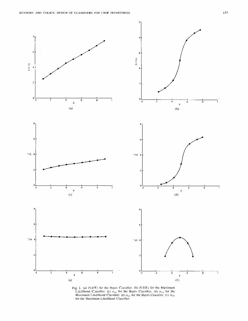
HEYDORN AND TAKACS: DESIGN OF CLASSIFIERS FOR CROP INVENTORIES
.9
153
x;::4w
x>-w
6
.2
oo .4
(a)
xo
ox
(b)
6
oo
x(c)
x(d)
.8
6
"2X .4.- . • • • • •
0'-- ...•..... ----' -'- -'- _o
x
(e)
O'----_~ -'- L- --'-- _o 6
x(f)
Fig. 1. (a) E(YIX) for the Bayes Classifier. (b) E(YIX) for the MaximumLikelihood Classifier. (c) "'IX for the Bayes Classifier. (d) "'IX for theMaximum Likelihood Classifier. (e) "'OX t()f the Bayes Classifier. (f) ""Xfor the Maximum Likelihood Classifier.
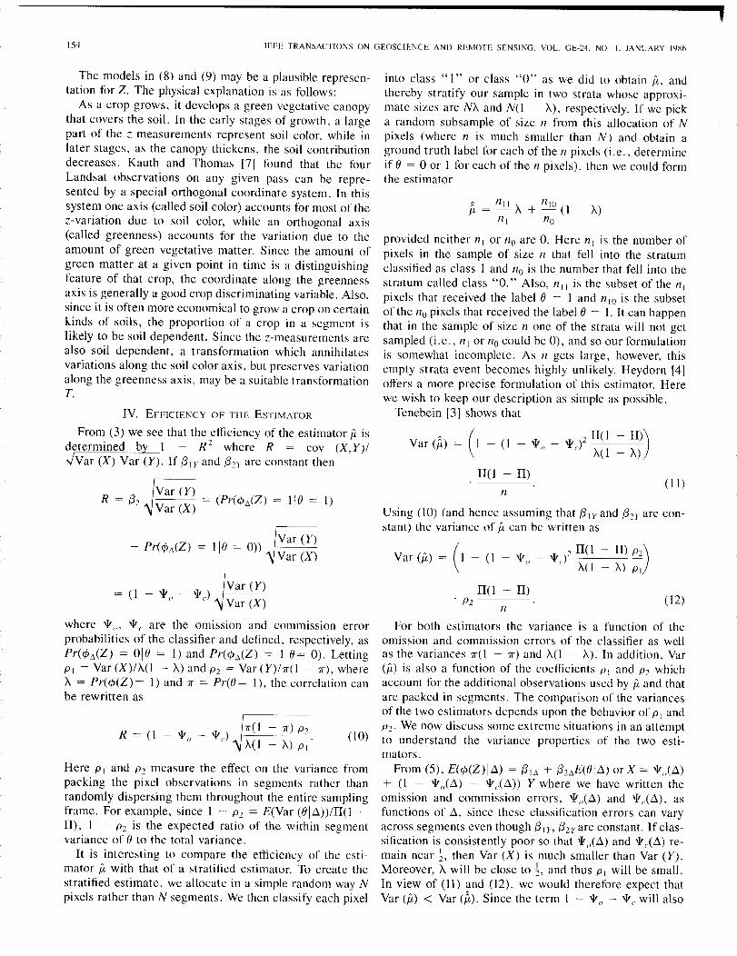
]54 IEEE TRANSACTIONS ON GEOSCIENCE AND REMOTE SENSING. VOL. GE-24. NO.1. JANUARY 1986
Var (Y)= (Pr(¢:1(Z) = 110 = 1)
Var(X)
IV. EFFICIENCY OF THE ESTIMATOR
From (3) we see that the efficiency of the estimator fi isdetermined by 1 - R 2 where R = cov (X, Y)/.JVar (X) Var (Y). If {3IY and (3n are constant then
(\ 1)
(\2)
- II) P2)- A) PI
17
(
J II( II - (\ - '11" - '¥J~
A(\
II(l - II)P2
(2 II(\ - II))
Var (A) = I - (\ - '11" - '11,) A(\ _ A)
II(\ - II)n
Var (fi) =
Using (10) (and hence assuming that {31Y and (3n are con-stant) the variance of fi can be written as
A = ~ A + 1710 (l - A)
171 no
provided neither 17 I or no are O. Here 171 is the number ofpixels in the sample of size n that fell into the stratumclassified as class 1 and no is the number that fell into thestratum called class "0." Also, 17 I I is the subset of the 17 I
pixels that received the label 0 = 1 and 17 10 is the subsetof the no pixels that received the label 0 = I. It can happenthat in the sample of size n one of the strata will not getsampled (i.e., 171 or no could be 0), and so our formulationis somewhat incomplete. As 17 gets large, however, thisempty strata event becomes highly unlikely. Heydorn [4Joffers a more precise formulation of this estimator. Herewe wish to keep our description as simple as possible.
Tenebein [3] shows that
into class "1" or class "0" as we did to obtain fi, andthereby stratify our sample in two strata whose approxi-mate sizes are NA and N(l - A), respectively. If we picka random subsample of size 17 from this allocation of Npixels (where n is much smaller than N) and obtain aground truth label for each of the 17 pixels (i.e., determineif 0 = 0 or I for each of the 17 pixels), then we could formthe estimator
Var (Y)
Var (X)
Var (Y)Var (X)
110=0))
(\ - '11" - '¥J
The models in (8) and (9) may be a plausible represen-tation for Z. The physical explanation is as follows:
As a crop grows, it develops a green vegetative canopythat covers the soil. In the early stages of growth, a largepart of the z-measurements represent soil color, while inlater stages, as the canopy thickens, the soil contributiondecreases. Kauth and Thomas [TI found that the fourLandsat observations on any given pass can be repre-sented by a special orthogonal coordinate system. In thissystem one axis (called soil color) accounts for most of thez-variation due to soil color, while an orthogonal axis(called greenness) accounts for the variation due to theamount of green vegetative matter. Since the amount ofgreen matter at a given point in time is a distinguishingfeature of that crop, the coordinate along the greennessaxis is generally a good crop discriminating variable. Also,since it is often more economical to grow a crop on certainkinds of soils, the proportion of a crop in a segment islikely to be soil dependent. Since the z-measurements arealso soil dependent, a transformation which annihilatesvariations along the soil color axis, but preserves variationalong the greenness axis, may be a suitable transformationT.
where '11", '¥C are the omission and commission errorprobabilities of the classifier and defined, respectively, asPr(¢:1(Z) = 010 = I) and Pr(¢:1(Z) = 110= 0). LettingPI = Var (X)/A(l - A) and P2 = Var (Y)/1f(1 - 1f), whereA = Pr(¢(Z)= 1) and 1f = Pr(O= 1), the correlation canbe rewritten as
Here P I and P2 measure the effect on the variance frompacking the pixel observations in segments rather thanrandomly dispersing them throughout the entire samplingframe. For example, since 1 - P2 = E(Var (OI.6.))/fI(1 -II), 1 - P2 is the expected ratio of the within segmentvariance of 0 to the total variance.
It is interesting to compare the efficiency of the esti-mator fi with that of a stratified estimator. To create thestratified estimate, we allocate in a simple random way Npixels rather than N segments. We then classify each pixel
1f(l - 1f) P2A(l - A) PI
(10)
For both estimators the variance is a function of theomission and commission errors of the classifier as wellas the variances 1f(1 - 1f) and A(1 - A). In addition, Var(fi) is also a function of the coefficients PI and P2 whichaccount for the additional observations used by fi and thatare packed in segments. The comparison of the variancesof the two estimators depends upon the behavior of PI andP2' We now discuss some extreme situations in an attemptto understand the variance properties of the two esti-mators.
From (5), E(¢(Z) 1.6.)= (31:1 + (32:1E(OI.6.)or X = '11,,(.6.)+ (1 - '11,,(.6.) - '¥c(.6.)) Y where we have written theomission and commission errors, '11,,(.6.)and '¥c(Li.) , asfunctions of .6., since these classification errors can varyacross segments even though {3 IY, (32 yare constant. If clas-sification is consistently poor so that '¥(}(.6.)and '¥c(Li.) re-main near ~, then Var (X) is much smaller than Var (Y).Moreover, ).,.will be close to t and thus P I will be small.In view of (11) and (12), we would therefore expect thatVar (fi) < Var (A). Since the term I - '¥() - '¥C will also
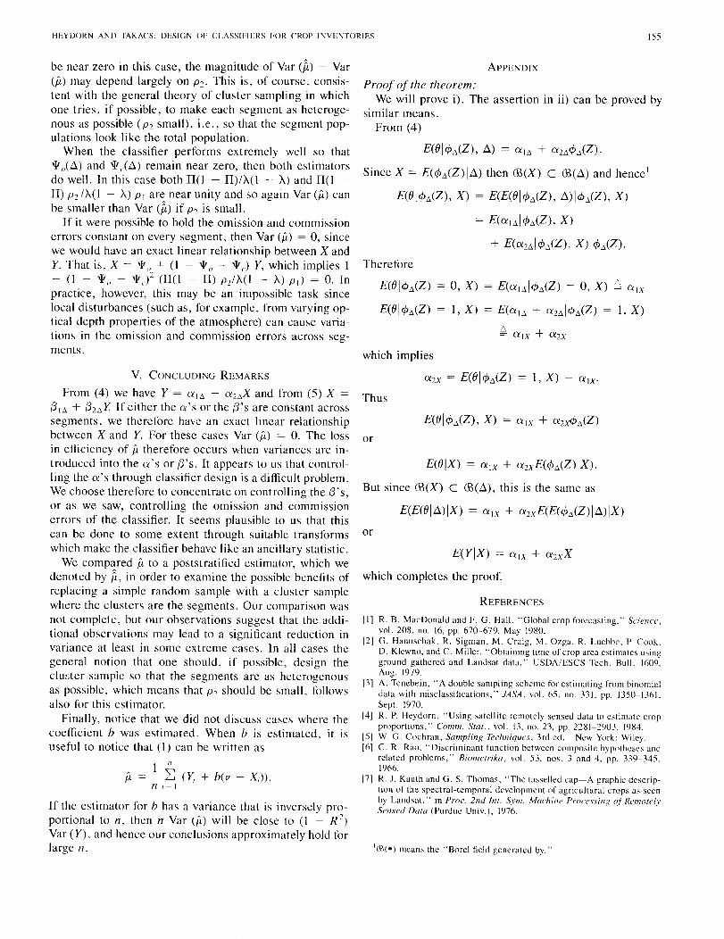
HEYDORN AND TAKACS: DESIGN OF CLASSIFIERS FOR CROP INVENTORIES 155
I, X) - alX'
0, X) = E(al2>I<t>2>(Z) = 0, X) ~ alX
I, X) = E(al2> + 0022>1<t>2>(Z) = I, X)
E(81<t>2>(Z)
E(81 <t>2>(Z)
Therefore
which implies
a2X = E(81<t>2>(Z)
or
REFERENCES
or
ApPENDIX
But since CB(X) C CB(Ll), this is the same as
Proof of the theorem:We will prove i). The assertion in ii) can be proved by
similar means.From (4)
which completes the proof.
Thus
'(£(-) means the "Borel field generated by."
E(81<t>2>(Z), Ll) = 0012>+ a22><t>2>(Z),
Since X = E(<t>2>(Z)ILllthen CB(X) C CB(Ll)and hence!
E(81<t>2>(Z),X) = E(E(81<t>2>(Z), Ll)I<t>2>(Z), X)
E(alJ.I<t>2>(Z),X)
+ E(a2D.I<t>L/Z), X) <t>D.(Z),
IIJ R. B. MacDonald and F. G. Hall, "Global crop forecasting." Science,vol. 208. no. 16, pp. 670-679, May 1980.
12J G. Hanusehak, R. Sigman. M. Craig. M. Ozga, R. Luebbe, P. Cook.D. Klewno, and C. Miller, "Obtaining time of crop area estimates usingground gathered and Landsat data," USDA/ESCS Tech. Bull. 1609,Aug. 1979.
13] A. Tenebein, "A double sampl ing scheme for estimating from binomialdata with misclassilications," JASA. vol. 65, no. 331. pp. 1350-1361.Sept. 1970.
14] R. P. Heydorn, "Using satellite remotely sensed data to estimate cropproportions," Comm. Stat., vol. 13, no. 23. pp. 2281-2903, 1984.
151 w. G. Cochran, Sampling Techniques, 3rd ed. New York: Wiley.16] C. R. Rao, "Discriminant function between composite hypotheses and
related problems," Biometrika, vol. 53, nos. 3 and 4, pp. 339-345,1966.
17] R. J. Kauth and G. S. Thomas, "The tasselled eap-A graphic descrip-tion of the spectral-temporal development of agricultural crops as seenby Landsat," in Proc. 2nd Int. Sym. Machine Processing or RemotelvSm.\·ed Data (Purdue Univ.), 1976.
be near zero in this case, the magnitude of Var (A) - Var(P-) may depend largely on P2' This is, of course, consis-tent with the general theory of cluster sampling in whichone tries, if possible, to make each segment as heteroge-nous as possible (P2 small), i.e., so that the segment pop-ulations look like the total population.
When the classifier performs extremely well so that'¥)Ll) and '¥JLl) remain near zero, then both estimatorsdo well. In this case both II(\ - II)/A(\ - A) and II(\ -I1) P2/A(\ - A) PI are near unity and so again Var (jl) canbe smaller than Var (A) if P2 is small.
If it were possible to hold the omission and commissionerrors constant on every segment, then Var (jl) = 0, sincewe would have an exact linear relationship between X andY. That is, X = '¥o + (\ - '¥o - '¥c) Y, which implies I- (I - '¥O - '¥,l (II(\ - II) P2/A(\ - A) PI) = 0. Inpractice, however, this may be an impossible task sincelocal disturbances (such as, for example, from varying op-tical depth properties of the atmosphere) can cause varia-tions in the omission and commission errors across seg-ments.
I ",jl = - ~ (Y, + b(v - Xi»'
n i~ I
V. CONCLUDIKG REMARKS
From (4) we have Y = 0012>+ a22>X and from (5) X =
{3I2>+ {322>Y If either the a's or the {3's are constant acrosssegments, we therefore have an exact linear relationshipbetween X and Y. For these cases Var (jl) = 0. The lossin efficiency of jl therefore occurs when variances are in-troduced into the a's or {3's. It appears to us that control-ling the a's through classifier design is a difficult problem.We choose therefore to concentrate on controlling the (3's,or as we saw, controlling the omission and commissionerrors of the classifier. It seems plausible to us that thiscan be done to some extent through suitable transformswhich make the classifier behave like an ancillary statistic.
We compared jl to a poststratified estimator, which wedenoted by A, in order to examine the possible benefits ofreplacing a simple random sample with a cluster samplewhere the clusters are the segments. Our comparison wasnot complete, but our observations suggest that the addi-tional observations may lead to a significant reduction invariance at least in some extreme cases. In all cases thegeneral notion that one should, if possible, design thecluster sample so that the segments are as heterogenousas possible, which means that P2 should be small, followsalso for this estimator.
Finally, notice that we did not discuss cases where thecoefficient b was estimated. When b is estimated, it isuseful to notice that (\) can be written as
If the estimator for b has a variance that is inversely pro-portional to n, then n Var (jl) will be close to (I - R2)Var (Y), and hence our conclusions approximately hold forlarge n.

]56 IEEE TRANSACTIONS ON GEOSCIENCE AND REMOTE SENSING, VOL. GE-24, NO. I, JANUARY 19S6
Richard P. Heydorn received thc B.KE. degreein electrical engineering and the M.A. degree inmathematics from the University of Akron and thePh.D. degree in statistics from Ohio State Uni-versity.
He joined the NASA Johnson Space Center in]974 and worked in a research capacity on LAC]Eand AgR]STARS. He also served as the sciencemanager of thc NASA program in MathematicalPattern Recognition and Image Analysis.
Helen C. Takacs received the Ph.D. degree in ap-plied statistics from the University of Alahama.
She is an Associate Professor of Computer Sci-ence at Mississippi State University, wherc she alsoserves as Coordinator of Graduate Programs inComputer Science. She has worked as a NASA-ASEE Fellow at the Johnson Space Center, Hous-ton, TX.
Dr. Takacs chairs the Professional Develop-ment Committec and Tutorial Weeks j()r the Edu-cation Board of the Association for ComputingMachinery.
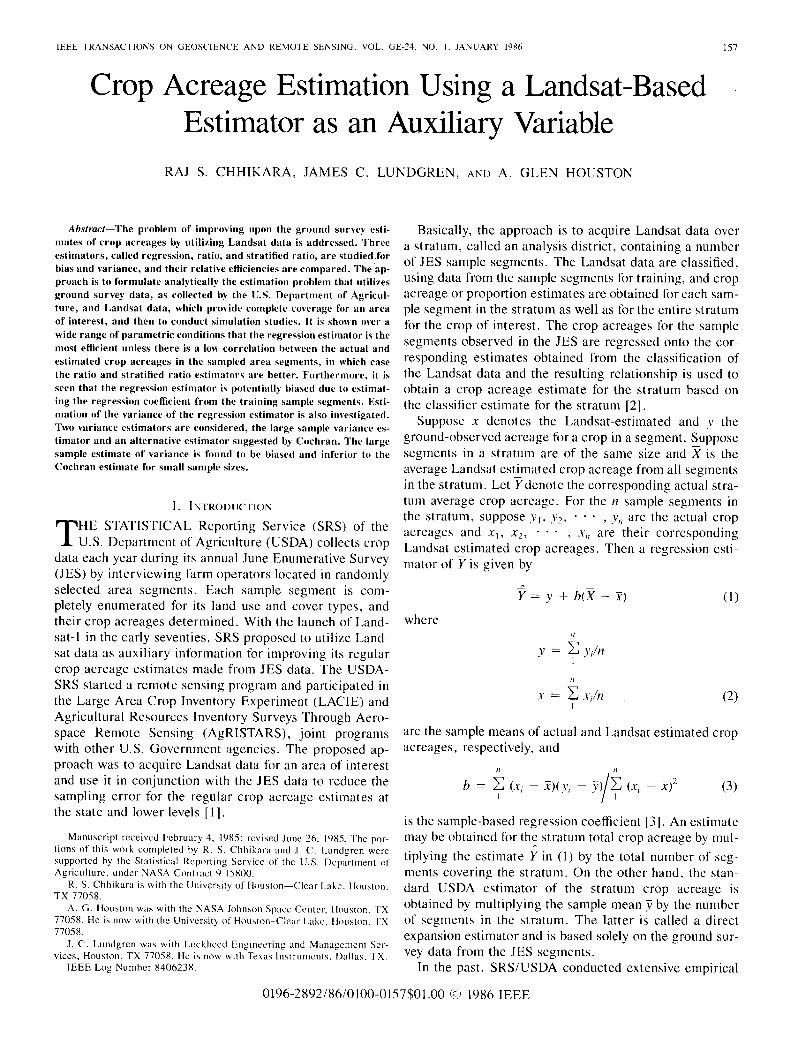
IEEE TRANSACTIONS ON GEOSCIENCE AND REMOTE SENSING. VOL. GE-24. NO.1. JANUARY 1986 157
Crop Acreage Estimation Using a Landsat-BasedEstimator as an Auxiliary Variable
RAJ S. CHHIKARA, JAMES C. LUNDGREN, AND A. GLEN HOUSTON
are the sample means of actual and Landsat estimated cropacreages, respectively, and
is the sample-based regression coefficient [3]. An estimatemay be obtained for th~ stratum total crop acreage by mul-tiplying the estimate Y in (I) by the total number of seg-ments covering the stratum. On the other hand, the stan-dard USDA estimator of the stratum crop acreage isobtained by multiplying the sample mean y by the numberof segments in the stratum. The latter is called a directexpansion estimator and is based solely on the ground sur-vey data from the JES segments.
In the past, SRS/USDA conducted extensive empirical
Basically, the approach is to acquire Landsat data overa stratum, called an analysis district, containing a numberof JES sample segments. The Landsat data are classified,using data from the sample segments for training, and cropacreage or proportion estimates are obtained for each sam-ple segment in the stratum as well as for the entire stratumfor the crop of interest. The crop acreages for the samplesegments observed in the JES are regressed onto the cor-responding estimates obtained from the classification ofthe Landsat data and the resulting relationship is used toobtain a crop acreage estimate for the stratum based onthe classifier estimate for the stratum [2].
Suppose x denotes the Landsat-estimated and Y theground-observed acreage for a crop in a segment. ~upposesegments in a stratum are of the same size and X is theaverage Landsat estimated crop acreage from all segmentsin the stratum. Let Y denote the corresponding actual stra-tum average crop acreage. For the n sample segments inthe stratum, suppose YI' Y2, ... 'Yll are the actual cropacreages and XI' X20 ••• ,X" are their correspondingLandsat estimated crop acreages. Then a regression esti-mator of Y is given by
(I)
(2)
(3)
"Y ~ vln, I
1
"X 2.: X /11
I
Y = y + h(X - x)
"h = 2.: (Xi - X)(Yi
I
where
Abstract-The problem of improving upon the ground survey esti-mates of crop acreages by utilizing Landsat data is addressed. Threeestimators, called regression, ratio, and stratified ratio, are studied .forbias and variance, and their relative efficiencies are compared. The ap-proach is to formulate analytically the estimation problem that utilizesground survey data, as collected by the U.S. Department of Agricul-ture, and Landsat data, which provide complete coverage for an areaof interest, and then to conduct simulation studies. It is shown over awide range of parametric conditions that the regression estimator is themost efficient unless there is a low correlation between the actual andestimated crop acreages in the sampled area segments, in which casethe ratio and stratified ratio estimators are beUer. Furthermore, it isseen that the regression estimator is potentially biased due to estimat-ing the regression coefficient from the training sample segments. Esti-mation of the variance of the regression estimator is also investigated.Two variance estimators are considered, the large sample variance es-timator and an alternative estimator suggested by Cochran. The largesample estimate of variance is found to be biased and inferior to theCochran estimate for small sample sizes.
I. INTRODUCTION
THE STATISTICAL Reporting Service (SRS) of theU.S. Department of Agriculture (USDA) collects crop
data each year during its annual June Enumerative Survey(JES) by interviewing farm operators located in randomlyselected area segments. Each sample segment is com-pletely enumerated for its land use and cover types, andtheir crop acreages determined. With the launch of Land-sat-I in the early seventies, SRS proposed to utilize Land-sat data as auxiliary information for improving its regularcrop acreage estimates made from JES data. The USDA-SRS started a remote sensing program and participated inthe Large Area Crop Inventory Experiment (LACIE) andAgricultural Resources Inventory Surveys Through Aero-space Remote Sensing (AgRISTARS), joint programswith other U.S. Government agencies. The proposed ap-proach was to acquire Landsat data for an area of interestand use it in conjunction with the JES data to reduce thesampling error for the regular crop acreage estimates atthe state and lower levels [11.
Manuscript received February 4. 19R5: revised June 26, 1985. The por-tions of this work completed by R. S. Chhikara and J. C. Lundgren wcresupported by the Statistical Reporting Service of the U. S. Department ofAgriculture, under NASA Contract 9-15800.
R. S. Chhikara is with the University of Houston-Clear Lake. Houston.TX 77058.
A. G. Houston was with the NASA Johnson Space Center, Houston, TX77058. He is now with the University of Houston- Clear Lake. Houston. TX77058.
J. C. Lundgren was with Lockhced Engineering and Management Ser-vices, Houston. TX 77058. Hc is now with Texas Instrumcnts. Dallas. TX.
IEEE Log Number 8406238.
0196-2892/86/0100-0157$01.00 © 1986 IEEE
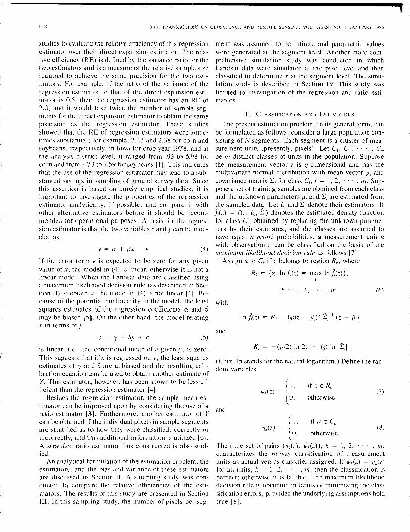
158 IEEE TRANSACTIONS ON GEOSCIENCE AND REMOTE SENSING, VOL. GE-24, NO. I, JANUARY 1986
If the error term E is expected to be zero for any givenvalue of x, the model in (4) is linear, otherwise it is not alinear model. When the Landsat data are classified usinga maximum likelihood decision rule (as described in Sec-tion II) to obtain x, the model in (4) is not linear [4]. Be-cause of the potential nonlinearity in the model, the leastsquares estimates of the regression coefficients IY and (3may be biased [5]. On the other hand, the model relatingx in terms of y
is linear, i.e., the conditional mean of e given y, is zero.This suggests that if x is regressed on y, the least squaresestimates of'Y and b are unbiased and the resulting cali-bration equation can be used to obtain another estimate ofY. This estimator, however, has been shown to be less ef-ficient than the regression estimator [4].
Besides the regression estimator, the sample mean es-timator can be improved upon by considering the use of ~ratio estimator 13]. Furthermore, another estimator of Ycan be obtained if the individual pixels in sample segmentsare stratified as to how they were classified, correctly orincorrectly, and this additional information is utilized [6].A stratified ratio estimator thus constructed is also stud-ied.
An analytical formulation of the estimation problem, theestimators, and the bias and variance of these estimatorsare discussed in Section II. A sampling study was con-ducted to compare the relative efficiencies of the esti-mators. The results of this study are presented in SectionIII. In this sampling study, the number of pixels per seg-
(8)
(7)
(6)
otherwise[
1.
0,
k= 1,2,'" ,m
Ki = -(p/2) In 27f - (1-) In It;!,
In ];(z) = Ki
[
I,lIk(Z) =
0, otherwise
Then the set of pairs (lIk(Z), 1/;k(Z» , k = 1,2, , m,characterizes the m-way classification of measurementunits as actual versus classifier assigned. If ih(z) = lIk(Z)for all units, k = I, 2, ... , m, then the classification isperfect: otherwise it is fallible. The maximum likelihooddecision rule is optimum in terms of minimizing the clas-sification errors, provided the underlying assumptions holdtrue [8].
and
and
with
(Here, In stands for the natural logarithm .) Define the ran-dom variables
ment was assumed to be infinite and parametric valueswere generated at the segment level. Another more com-prehensive simulation study was conducted in whichLandsat data were simulated at the pixel level and thenclassified to determine x at the segment level. The simu-lation study is described in Section IV. This study waslimited to investigation of the regression and ratio esti-mators.
II. CLASSIFICATION AND ESTIMATORS
The present estimation problem, in its general form, canbe formulated as follows: consider a large population con-sisting of N segments. Each segment is a cluster of mea-surement units (presently, pixels). Let C]. C2, ••• , Cm
be m distinct classes of units in the population. Supposethe measurement vector z is q-dimensional and has themultivariate normal distribution with mean vector J-Li andcovariance matrix Ei for class Ci, i = 1, 2, ... , m. Sup-pose a set of training samples are obtained from each classand the unknown parameters J-Li and Ei are estimated fromthe sampled data. Let ili and t; denote their estimators. If];(z) = fez, ili, t) denotes the estimated density functionfor class Ci, obtained by replacing the unknown parame-ters by their estimates, and the classes are assumed tohave equal a priori probabilities, a measurement unit uwith observation z can be classified on the basis of themaximum likelihood decision rule as follows [7]:
Assign u to Ck if z belongs to region Rko where
Rk = {z: In lk(z) = max In ];(z)},
(5)
(4)
x = 'Y + by + e
y = IY + (3x + E.
studies to evaluate the relative efficiency of this regressionestimator over their direct expansion estimator. The rela-tive efficiency (RE) is defined by the variance ratio for thetwo estimators and is a measure of the relative sample sizerequired to achieve the same precision for the two esti-mators. For example, if the ratio of the variance of theregression estimator to that of the direct expansion esti-mator is 0.5, then the regression estimator has an RE of2.0, and it would take twice the number of sample seg-ments for the direct expansion estimator to obtain the sameprecision as the regression estimator. These studiesshowed that the RE of regression estimators were some-times substantial; for example, 2.43 and 2.38 for corn andsoybeans, respectively, in Iowa for crop year 1978, and atthe analysis district level, it ranged from .93 to 5.98 forcorn and from 2.73 to 7.59 for soybeans [I]. This indicatesthat the use of the regression estimator may lead to a sub-stantial savings in sampling of ground survey data. Sincethis assertion is based on purely empirical studies, it isimportant to investigate the properties of the regressionestimator analytically, if possible, and compare it withother alternative estimators before it should be recom-mended for operational purposes. A basis for the regres-sion estimator is that the two variables x and y can be mod-eled as
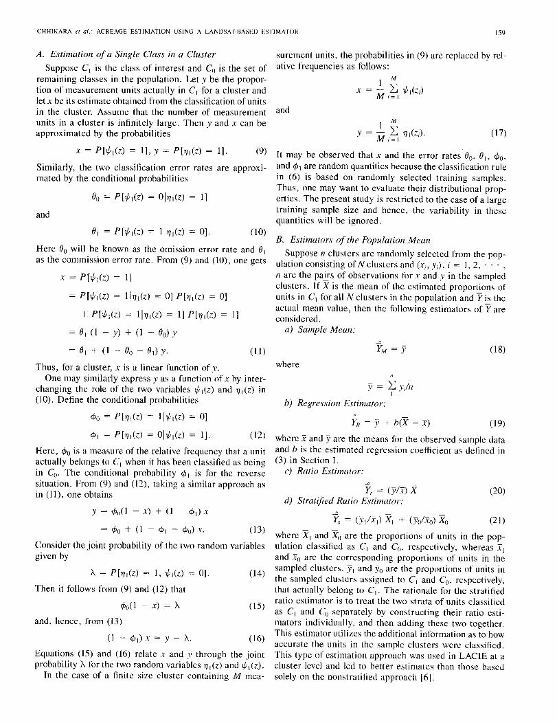
CHHIKARA et ai.: ACREAGE ESTIMATION USING A LANDSAT-BASED ESTIMATOR 159
A. Estimation of a Single Class in a Cluster
Suppose CI is the class of interest and Co is the set ofremaining classes in the population. Let y be the propor-tion of measurement units actually in CI for a cluster andlet x be its estimate obtained from the classification of unitsin the cluster. Assume that the number of measurementunits in a cluster is infinitely large. Then y and x can beapproximated by the probabilities
surement units, the probabilities in (9) are replaced by rel-ative frequencies as follows:
1 Mx = - ~ ~ [(Zi)
Mi='and
(17)
Similarly, the two classification error rates are approxi-mated by the conditional probabilities
and
x = P[~J(z) = 1], Y = P[1)I(Z) = 1]. (9) It may be observed that x and the error rates ()o, ()J, ¢o,and ¢, are random quantities because the classification rulein (6) is based on randomly selected training samples.Thus, one may want to evaluate their distributional prop-erties. The present study is restricted to the case of a largetraining sample size and hence, the variability in thesequantities will be ignored.
Here ()o will be known as the omission error rate and ()Ias the commission error rate. From (9) and (10), one gets
x = P[~I(Z) = 1]
= P[~J(z) = ll1)J(z) = 0] P[1)I(Z) = 0]
+ P[~1(Z) = ll1),(z) = 1] P[1),(z) 1]
= ()I (1 - y) + (1 - ()o) y
= ()1 + (1 - ()o - ()J) y. (11)
B. Estimators of the Population Mean
Suppose n clusters are randomly selected from the pop-ulation consisting of N clusters and (Xi' y;), i = 1,2, ... ,n are the paE's of observations for x and y in the sampledclusters. If X is the mean of the estimated proportions ofunits in C] for all N clusters in the population and Y ~ theactual mean value, then the following estimators of Yareconsidered.
a) Sample Mean:
(18)
Consider the joint probability of the two random variablesgiven by
A. = P[1)I(Z) = 1, ~,(z) = 0]. (14)
Then it follows from (9) and (12) that
(20)
(19)
(21)
YR = Y + b(X - x)
Yr = (y/x) Xd) Stratified Ratio Estimator:
b) Regression Estimator:
where
where x and yare the means for the observed sample dataand b is the estimated regression coefficient as defined in(3) in Section I.
c) Ratio Estimator:
y = ~ y/nI
11
where X, and Xo are the proportions of units in the pop-ulation classified as C, and Co, respectively, whereas XIand Xo are the corresponding proportions of units in thesampled clusters. YI and Yo are the proportions of units inthe sampled clusters assigned to C, and Co, respectively,that actually belong to CI. The rationale for the stratifiedratio estimator is to treat the two strata of units classifiedas C[ and Co separately by constructing their ratio esti-mators individually, and then adding these two together.This estimator utilizes the additional information as to howaccurate the units in the sample clusters were classified.This type of estimation approach was used in LACIE at acluster level and led to better estimates than those basedsolely on the nonstratified approach [6].
(13)
(16)
(15)
Thus, for a cluster, x is a linear function of y.One may similarly express y as a function of x by inter-
changing the role of the two variables ~,(z) and 1), (z) in(10). Define the conditional probabilities
¢o = P[1),(z) = ll~,(z) = 0]
¢, = P[1),(z) = Ol~,(z) = 1]. (12)
Here, ¢o is a measure of the relative frequency that a unitactually belongs to C, when it has been classified as beingin Co. The conditional probability ¢ I is for the reversesituation. From (9) and (12), taking a similar approach asin (11), one obtains
y = ¢0(1 - x) + (1 - ¢,) x
Equations (15) and (16) relate x and y through the jointprobability A. for the two random variables 1),(z) and ~,(z).
In the case of a finite size cluster containing M mea-
¢o( 1 - x) = A.
and, hence, from (13)
(1 - ¢I) x = y - A..

160 IEEE TRANSACTIONS ON GEOSCIENCE AND REMOTE SENSING, VOL. GE-24, NO. L JAJ\'lJARY 1986
Y, = ~. + 1t../(x(1 ~ x))] (x ~ X) (22)
In the Appendix, it is shown that the stratified ratio es-timator can be expressed as
where S2 is the population variance and 1/ is the samplesize. An estimate of the variance in (23) is given hy
(29)IN I I N 1.
1/2, -- 1 -, _ J
gl = --~ 2..: (x, - .x) 1-- 2..: (Xi - xtN - I \ N ~ I ]
is the relative skewness of the distribution of Xi in the pop-ulation.
c) In general, the ratio estimator is biased and is nomore efficie'lt than the regression estimator. The bias andvarianee of Y, with Xi assumed known are discussed in [1,p. 160]. When the Xi are estimated, the properties of Y,have not been investigated; however, in the limiting casethese are expected tq be the same as in [31.
d) The estimator Y, is new and its properties need to beestabl ished, In the appendix, we deriv,e expressions of thebias and the mean squared error of Y, to terms of order1/- I. It is shown that in tl:le limit, as the sample size nincreases without bound, Y, has the ,same bias and meansquared error as the ratio estimator Y,.
where
The variance estimator in (27) generally underestimatesthe t rue variance for small sample sizes [ 10]. Another var-iance estimator based on a formula on p. 197 in [31, givennext, is considered to be superior for small sample sizes.
V(l~'R) = [(I - nlN) s;,/n] [I + lI(n - 3) + 2g~/n2]
(28)
(23)vO\,) = (I - n/N) S2/1/
C. Sampling Properties of the EstimatorsFor the standard survey estimation case, the bias and
variance for estimators a)-c) are well known [3J. Thus,we will state here the main results, skipping details unlesswarranted. A
a) The estimator ~w is simply the sample mean andhence it is unbiased and has variance
where t.. is the average of the t..i for the sampled c1ustfrs,t..i is the joint probability of (14) for cluster i, and Y, isthe ratio estimator given in (20). Note that the sccond termon the right side in (22) is analogous ~) that in (19) for theregression estimator. The coefficient t../(x(1 - x)) is a rel-ative measure of the discrepancy between the actual andclassifier assigned labels for units. II' there is completeagreement~ that is ev~ry s'1mple unit is correctly classi-fied, then t.. = ° and Y, = Y,; otherwise the second termaccounts for the fallibility of the classification rule.
11
where
s~ 2..: (Yi - .vi/(n - 1)\
.Vi = Y + h(Xi - x).
III. AN EVALUATION OF ESTIMATORS
In this section we discuss a certain sampling study con-ducted to evaluate the above estimators. For simplicity, werestrict attention to a two-class case in which the mea-surement vector 2 is distributed normally with mean vec-tors /J.\ and /J.o for C] and Co, respectively, and commoncovariance matrix L. By a set of linear transformations,the class structure can be obtained in the canonical formso that the vector 2 can be assumed to have class meanvectors (-11/2, 0, 0, ... , 0) and (11/2, 0, ... , 0) forC1 and Co, respectively, and common covariance matrixI, where
11 = [(/J.\ - /J.fl)' L ] (/J.I ~ /J.o)]112 (30)
is the Mahalanobis distance between the two classes andis a measure of class separability. When 11 is known, themaximum likelihood classification rule is to classify ameasurement unit in CI if 21 < 0, and in Co otherwise,where 2 I is the first component of measurement vector 2.
Observe that 2\ has a univariate normal distribution andthe omission and commission error rates for the popula-tion arc each equal to <1>( -11/2), where <I> denotes the cu-mulative distribution function for the standard normal [II].
For the stratified ratio estimator, the classification errorrates must be evaluated for individual clusters. Since thecluster size is assumed infinitely large, the class distri-butions for each cluster can be approximated by the nor-mal distribution. For cluster i, let ~ie and (t + l1;)e bethe mean vectors of the measurement vector 2 for C1 andCo, respectively, where e = (I. n, 0, ... , 0) is a q X Ivector and I is the common covariance matrix. This dis-
(27)
(24)
(25)S2 = 2..: (Yi - ,;)2/(n ~ I).\
~ - ")
v(Yw) = (I - 1//N) .\~-/1/
where N is the population size and
h) The regression estimator YR can be used even whenthe underlying regression function is not strictly linear,provided a sample plot of the Yi against Xi appears approx-imately linear [3, p. I93J. Presently, the regressor valuesXi are estimated and therefore;, the previously known re-sults for bias and variance of YR as given in [3] hold trueonly if the Xi are assumed known. Recently, Hung [91 in-vestigated the case where the Xi are estimate~ and showedthat under certain conditions, the estimator YR with the Xi
estimated has the same limiting distribution as when theXi are known. A
The bias of YR is of order I/n, and its variance for largen is given by
v(YR) = (I - n/N) S2 (I - R2)/n (26)
where R is the population correlation coefficient betweenthe Yi and Xi' An estimate of this variance using the largesample variance formula given in [3, p. 194] is given by
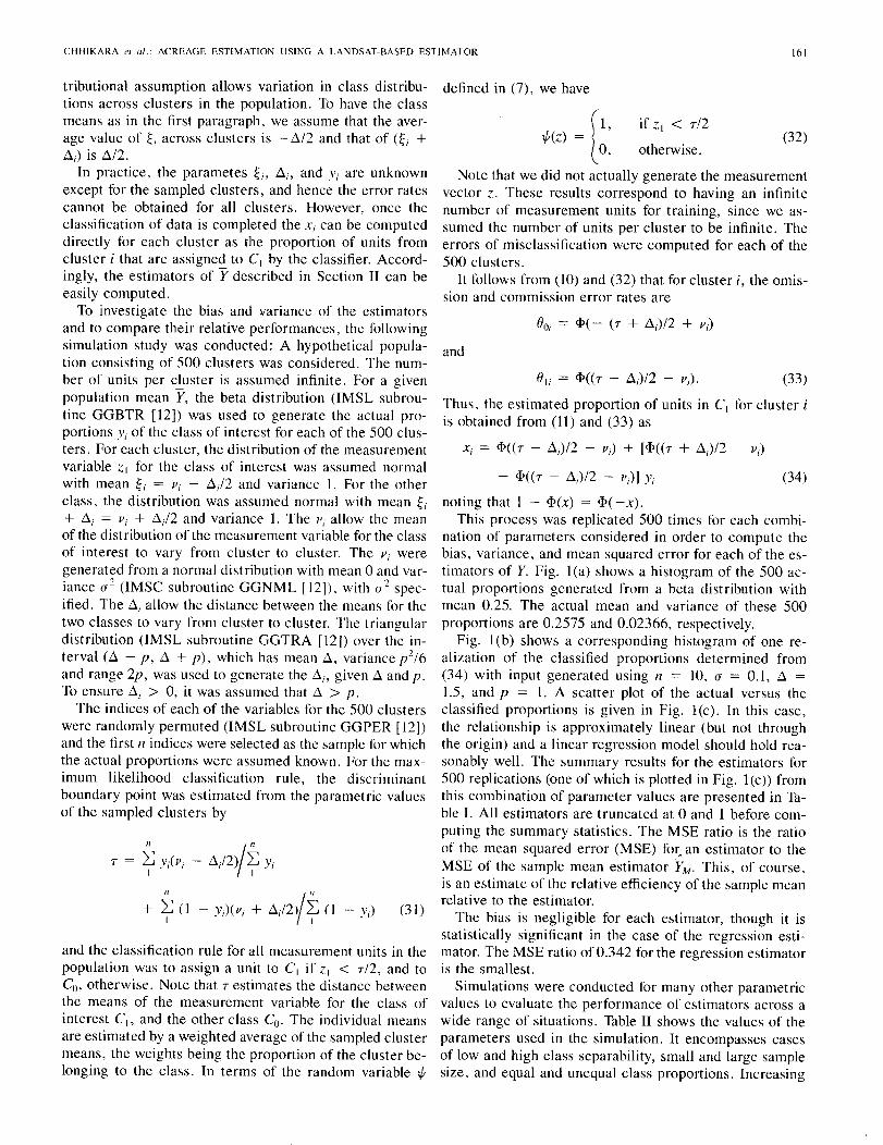
CHHIKARA el al.: ACREAGE ESTIMATION USING A LANDSAT~BASED ESTIMATOR 161
and the classification rule for all measurement units in thepopulation was to assign a unit to C] if z, < 7/2, and toCo, otherwise. Note that 7 estimates the distance betweenthe means of the measurement variable for the class ofinterest C], and the other class Co. The individual meansare estimated by a weighted average of the sampled clustermeans, the weights being the proportion of the cluster be-longing to the class. In terms of the random variable 1/;
tributional assumption allows variation in class distribu-tions across clusters in the population. To have the classmeans as in the first paragraph, we assume that the aver-age value of ~i across clusters is - t!./2 and that of (t +t!.i) is t!./2.
In practice, the parametes ~i, t!.i, and Yi are unknownexcept for the sampled clusters, and hence the error ratescannot be obtained for all clusters. However, once theclassification of data is completed the Xi can be computeddirectly for each cluster as the proportion of units fromcluster i that are assigne~ to C, by the classifier. Accord-ingly, the estimators of Y described in Section II can beeasily computed.
To investigate the bias and variance of the estimatorsand to compare their relative performances, the followingsimulation study was conducted: A hypothetical popula-tion consisting of 500 clusters was considered. The num-ber of units per cluster is assumed infinite. For a givenpopulation mean Y, the beta distribution (IMSL subrou-tine GGBTR [12]) was used to generate the actual pro-portions Yi of the class of interest for each of the 500 clus-ters. For each cluster, the distribution of the measurementvariable z, for the class of interest was assumed normalwith mean ~i = Vi - t!.J2 and variance 1. For the otherclass, the distribution was assumed normal with mean t+ t!.i = Vi + t!.J2 and variance 1. The Vi allow the meanof the distribution of the measurement variable for the classof interest to vary from cluster to cluster. The Vi weregenerated from a normal distribution with mean 0 and var-iance (J2 (lMSC subroutine GGNML [12]), with (J2 spec-ified. The t!.i allow the distance between the means for thetwo classes to vary from cluster to cluster. The triangulardistribution (IMSL subroutine GGTRA [12]) over the in-terval (t!. - p, t!. + p), which has mean t!., variance li/6and range 2p, was used to generate the t!.i, given t!. and p.To ensure t!.i > 0, it was assumed that t!. > p.
The indices of each of the variables for the 500 clusterswere randomly permuted (IMSL subroutine GGPER [12])and the first n indices were selected as the sample for whichthe actual proportions were assumed known. For the max-imum likelihood classification rule, the discriminantboundary point was estimated from the parametric valuesof the sampled clusters by
defined in (7), we have
(32)
(33)(J1i = <1>((7 - t!.J/2 - vJ.
and
[
I,1/;(z) =
0, otherwise.
Note that we did not actually generate the measurementvector z. These results correspond to having an infinitenumber of measurement units for training, since we as-sumed the number of units per cluster to be infinite. Theerrors of misclassification were computed for each of the500 clusters.
It follows from (10) and (32) that for cluster i, the omis-sion and commission error rates are
Thus, the estimated proportion of units in C, for cluster iis obtained from (11) and (33) as
Xi = <1>((7 - t!.i)/2 - vJ + [<1>((7 + t!.J/2 - vJ
- <1>((7 - t!.Y2 - vJ] Yi (34)
noting that I - <I>(x) = <1>( - x).This process was replicated 500 times for each combi-
nation of parameters considered in order to compute thebias, varian~e, and mean squared error for each of the es-timators of Y. Fig. I (a) shows a histogram of the 500 ac-tual proportions generated from a beta distribution withmean 0.25. The actual mean and variance of these 500proportions are 0.2575 and 0.02366, respectively.
Fig. I (b) shows a corresponding histogram of one re-alization of the classified proportions determined from(34) with input generated using n = 10, (J = 0.1, t!. =1.5, and p = 1. A scatter plot of the actual versus theclassified proportions is given in Fig. I(c). In this case,the relationship is approximately linear (but not throughthe origin) and a linear regression model should hold rea-sonably well. The summary results for the estimators for500 replications (one of which is plotted in Fig. 1(c» fromthis combination of parameter values are presented in Ta-ble I. All estimators are truncated at 0 and I before com-puting the summary statistics. The MSE ratio is the ratioof the mean squared error (MSE) for, an estimator to theMSE of the sample mean estimator YM. This, of course,is an estimate of the relative efficiency of the sample meanrelative to the estimator.
The bias is negligible for each estimator, though it isstatistically significant in the case of the regression esti-mator. The MSE ratio of 0.342 for the regression estimatoris the smallest.
Simulations were conducted for many other parametricvalues to evaluate the performance of estimators across awide range of situations. Table II shows the values of theparameters used in the simulation. It encompasses casesof low and high class separability, small and large samplesize, and equal and unequal class proportions. Increasing
(31)
n ( n~ y·(v - t!./2) ~ y
¥ {I l 0/ I, ,n ( n+ ~ (1 - yJ(Vi + t!.J2) ~ (1 - yJ, I
7=

162 IEEE TRANSACTIONS ON GEOSCIENCE AND REMOTE SENSING, VOL. GE-24, NO. I, JANUARY 1986
1I,i11I1.B8 11.16 11,24 11.32 11.41111.48 II.SG 11.6411.72 II.EIIlII.IE 11.96
(a)
1I.i11I1.B8 11.16 1l.24 11.32 11.41111.48 II.SG 11.64 11.72 II.EIIl II.IE 1l.96
(b)
AeT II.UAL
II.PR0P II.0RTI0ri5
II.
11.11 11.2 11.4 11.6 11.8 1.11
(e)
Fig. 1. Histograms and scatter plot of class proportions when Y - 0.25, a=0.1,1l = 1.5,p = l,and/1 = 10.
I
TABLE ISLMMARY STATISTICS FOR 500 REPLICATIOI'S WITH Y = 0.25, /1 = 10, a =
0.1. II = 1.5, AND P = 1.0
Estimator Bi as Vari ance MSE MSE Rat i 0 t-Stati stic
Sampl e Mean .0020 .0021 .0021 1 .000 .97Regress; on -.0033 .0007 .0007 .342 -2.77Rat; 0 -.0003 .0009 .0009 .425 - .19Stratified Ratio .0011 .0012 .0012 .595 .72
values of p or a give rise to larger variability in separabil-ity, resulting in lower correlation between the Xi and Yi'
In each simulation run, the square of the correlationcoefficient between the Xi and Yi, R 2, was computed forboth the population and the sample. Variation in the pop-ulation correlation coefficient arises due to the decisionrule for the maximum likelihood classifier varying fromsample to sample for the 500 replications. Figs. 2 and 3summarize the MSE ratios of the estimators as a function
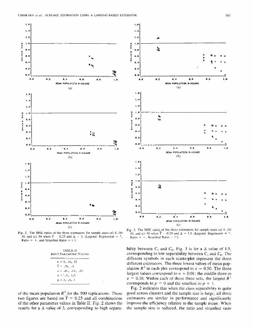
CHHIKARA el ai.: ACREAGE ESTIMATION USING A LANDSAT-BASED ESTIMATOR 163
~AN POPULATION R-SQUARE
(c)
Fig. 3. The MSE ratios of the three estimators for sample sizes (a) 4. (b)10, and (c) 30 when Y = 0,25 and Ll. = 1.5. (Legend: Regression = *Ratio = +, Stratified Ratio = Ii).
HEAN POPI.JLATION R-SOUARE
(a)
~AN POPULATION R-SQUARE
(b)
I.e
D D...
I.B
1.8
•
... .
!tI D D 0
.••..+ + +
,.
~ + + +
B.B
8.8
B.8
D
•..
+•
D
D
•+
e.8
8,8
8.8
e'.•
e:4
e.4
B.2
8.2
B.2
1.
8.
B.8
I.JI.
H 1.asE
B .8
B.8
1.2
1.2
B.B
I.
RAT B.6Io
8.B
8 .•
B.2
~ 1.8SE
B.8
B .8
B.e
e.2
1.
B.
8.2
B.8
1.
1.2
RAT B.6Ia
~ loBSE
RAT 8 •Ia
1.8
I.
1.2
~ 1.8SE
8.8RAT 8.8 •I ••a
8.
8.2
III~
B.8 ~B.B B.2 B.4 B.lI B.8 loB
/lEAN POPULATION R-SQUARE
(a)
I.
1.4
1.2
~ 1 ••SE
B.8RAT B.8I0
8.4 * ••• ::>;J
e.2
B.B ~e.8 e.2 e.4 B.8 B.8 loB
~EAN POPULATION R-SQUARE
(b)
1.8
I..
1.2
~ 1.8SE
e.8RAT 8.8Ia
8 .• ,~B.2
B.8 ~8.B B.2 8.4 8.8 8.8 loB
~EAN POPULATION R-SQUARE
(c)
Fig. 2. The MSE ratios of the three estimators for sample sizes (a) 4, (b)10, and (c) 30 when Y = 0.25 and Ll. = 3. (Legend: Regression = *,Ratio = +, and Stratified Ratio = L I).
TABLE IIINPUT PARAMETRIC VALUES
n = 4, 10, 30
Y = .25, .5
cr = .01, .10, .50
~=1.5,3.0
P = 0, .5, 1
of the mean population R2Jor the 500 replications. Thesetwo figures are based on Y = 0.25 and all combinationsof the other parameter values in Table II. Fig. 2 shows theresults for a Ll value of 3, corresponding to high separa-
bility between C1 and Co' Fig. 3 is for a Ll value of 1.5,corresponding to low separability between C1 and Co. Thedifferent symbols in each scatterplot represent the threedifferent estimators. The three lowest values of mean pop-ulation R2 in each plot correspond to (J = 0.50. The threelargest values correspond to (J = 0.01; the middle three to(J = 0.10. Within each of these three sets, the largest R 2
corresponds to p = 0 and the smallest to p = 1.Fig. 2 indicates that when the class separability is quite
good across clusters and the sample size is large, all threeestimators are similar in performance and significantlyimprove the efficiency relative to the sample mean. Whenthe sample size is reduced, the ratio and stratified ratio
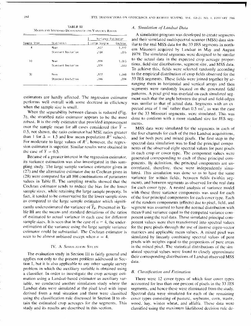
164 IEEE TRANSACTIONS ON GEOSCIENCE AND REMOTE SE;\ISING. VOL. GE·24. NO. I, Ji\t\UARY 1980
Variance Estimator
IV. A SIMULATIONSTUDY
TABLE IIIMEANS AND STA'mARD DEVIATIONS Of, THE YARL\NCE RATIOS
The evaluation study in Section III is fairly general andapplies not only to the present problem addressed in Sec-tion I, but it is also applicable to any other sample surveyproblem in which the auxiliary variable is obtained usinga classifier. In order to investigate the crop acreage esti-mation using a Landsat-based estimator as auxiliary var-iable, we conducted another simulation study where theLandsat data were simulated at the pixel level with inputderived from a real situation and these were classifiedusing the classification rule discussed in Section II to ob-tain the estimated crop acreages for the segments, Thisstudy and its results are described in this section,
A, Simulation of Landsat Data
A simulation program was developed to create segmentsand their simulated multispectral scanner (MSS) data sim-ilar to the real MSS data for the 33 JES segments in north-ern Missouri acquired by Landsat in May and August1979, The simulated segments were designed to be similarto the actual data in the expected crop acreage propor-tions, field size distributions, segment size. and MSS data,To achieve this, lIelds were selected randomly accordingto the empirical distribution of crop fields observed for the33 JES segments, These fields were joined together by ar-ranging them in horizontal and vertical arrays and thensegments were randomly located on the generated fieldpatterns, A pixel grid was overlaid on each simulated seg-ment such that the angle between the pixel and field edgeswas similar to that of actual data, Segments with an ex-pected area of I mi2 rather than 0,5 mi2
, as was the casefor the 33 Missouri segments, were simulated, This wasdone to conform with a more standard size for JES seg-ments.
MSS data were simulated for the segments in each ofthe four channels for each of the two Landsat acquisitions,and for both pure and mixed pixels, The first step in thespectral data simulation was to find the principal compo-nents of the observed eight spect ral values for pure pixelsin each crop or cover type, The component values weregenerated corresponding to each of these principal com-ponents, By definition, the principal components are un-correlated, therefore, these were independently simu-lated, This simulation was done so as to have the samevariance for within fields, between fields (within seg-ment), and between segments as observed for the real datafor each cover type. A nested analysis of variance modelwith these three variance components was used for eachof the four principal components for each cover type. Eachof the random components (effects) due to pixel, field, andsegment was assumed to have the normal dist ribution withmean 0 and variance equal to the computed variance com-ponent using the real data, These simulated principal com-ponent values were then transformed into spectral valuesfor the pure pixels through the use of inverse eigen-vectormatrices and applicable mean values. A mixed pixel wassimulated by linearly combining spectral values of purepixels with weights equal to the proportions of pure areasin the mixed pixel. The statistical distributions of the sim-ulated spectral values were found to closely approximatetheir corresponding distributions of Landsat observed MSSdata,
B. Class(fication and Estimation
There were 12 cover types of which four cover typesaccounted for less than one percent of pixels in the 33 JESsegments, and hence these were eliminated from the study,Spectral data were simulated for each of the remainingcover types consisting of pasture, soybeans, corn, waste,wood, hay, winter wheat, and alfalfa, These data wereclassified using the maximum likelihood decision rule de-
Stati sties Large Samp1 e Coc h ran
Mean .602 1.227
Standard Deviation .108 .215
Mean .884 1 .01 5
Standard Deviation .074 ,083
Mean .972 1.000
Standard Deviation .096 .094
Samp1 e Si ze
30
10
estimators are hardly affected, The regression estimatorperforms well overall with some decrease in efficiencywhen the sample size is small.
When the separability between classes is reduced (Fig,3), the stratified ratio estimator appears to be the mostrobust. It is the only estimator that provided improvementover the sample mean for all cases considered (for Y =0,5, not shown. the ratio estimator had MSE ratios greaterthan I for ~ = 1.5 and low mean population R2 values),For moderate to large values of R 2, however, the regres-sion estimat,.<:>ris superior. Similar results were obtained inthe case of Y = OS
Because of a greater interest in the regression estimator,its variance estimation was also investigated in this sam-pling study, The large sample variance estimator given in(27) and the alternative estimator due to Cochran given in(28) were computed for all 108 combinations of parametervalues in Table II. The sampling results showed that theCochran estimator tends to reduce the bias for the lowersample sizes, while retaining the large sample property, Infact, it tended to be conservative for the lower sample sizesas compared to the large sample estin;ator which signifi-cantly underestimated the variance of YR, Presented in Ta-ble III are the means and standard deviations of the ratiosof estimated to actual variance in each case for differentsample sizes. It is seen that in the case of II = 4, the under-estimation of the variance using the large sample varianceestimator could be substantial. The Cochran estimator isseen to be almost unbiased except when 11 = 4,
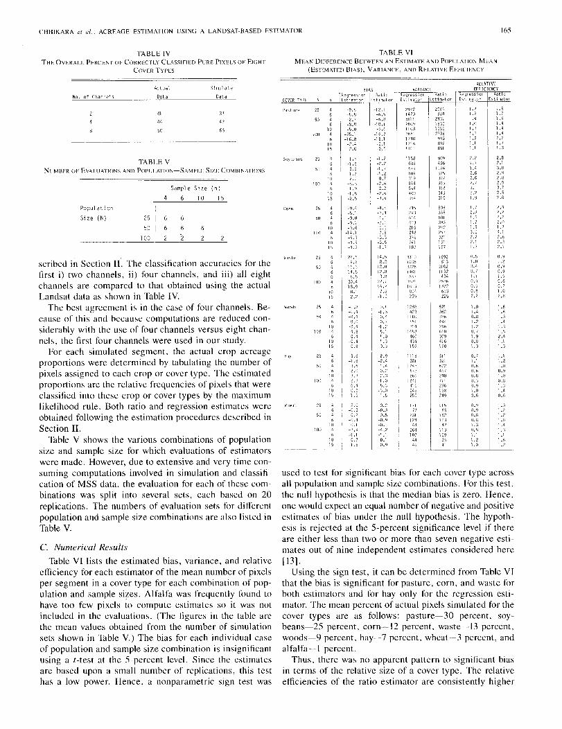
CHHIKARA el al.: ACREAGE ESTIMATION USlNG A LANDSAT-BASED ESTIMATOR 165
TABLE IVTHE OVERALL PERCE~T OF CORRECTLY CLASSIFIED PURE PIXELS OF EIGHT
COVER TYPES
TABLE VIMEAN DIFFERENCE BETWEEN A'l ESTIMATE A'lD POPULATIO'l MEAN
(ESTIMATED BIAS), V ARIA'lCE, AND RELATIVE EFFICIENCY
Actual Si lTlul atert
No. of Channels Data DataCOVER il'PE
41 37Pilsture 2\
44 4:? 50
50 65100
BIASegresslan atlo
Estimator Estimator'
-9.6 -12.1-6.t) -6.5-2.7 -6.8-8.R -10.1-5.0 -5.6
-25.1 -16.7-16.8 -le.1
-2.4 -2,12.0 -D,S
2.82.13.02.92.82.93.72.\2.0
2.11.71.42.51.62.73.12.21.9
1.2 1.51.2 1.7
.9 1,61.0 1.41.3 1.41.3 1.41.9 2.21.1 1.71.1 1.3
RELAHV[EFFICIENCY
egressl0n atloEstimator Estimator
905462345310
909496
VA~IANCEecreSSlon atlo
Est"'toe_I' E~toe297214/J50112601j11 0336bl1240 99312:'6 8Q21021 851
I-1,2 58-2.2-1.7 I 1679-1.2 609
0.7 319-2.6 21',4
2.2 544-2.6 40,:)-3.6 354
-1.8-2.5
1.5-1.25.6
4646
1046
1015
Soybeans 25 45
50 46
10100 4
6101\
TABLE VNUMBER OF EVAI.UATIONS AND POI'CLATION-SAMPI.F SIZE C()MBI~ATI()NS
Samp 1 e Size (n)
4 6 10 15
used to test for significant bias for each cover type acrossall population and sample size combinations. For this test,the null hypothesis is that the median bias is zero. Hence,one would expect an equal number of negative and positiveestimates of bias under the null hypothesis. The hypoth-esis is rejected at the 5-percent significance level if thereare either less than two or more than seven negative esti-mates out of nine independent estimates considered here113] .
Using the sign test, it can be determined from Table VIthat the bias is significant for pasture, corn, and waste forboth estimators and for hay only for the regression esti-mator. The mean percent of actual pixels simulated for thecover types are as follows: pasture-30 percent, soy-beans-25 percent, corn-12 percent, waste-13 percent,woods-9 percent, hay-7 percent, wheat-3 percent, andalfalfa-l percent.
Thus, there was no apparent pattern to significant biasin terms of the relative size of a cover type. The relativeefficiencies of the ratio estimator are consistently higher
1.61.61.31.41.31.52.41.11.3
1.31.11.21.01.4'1.31.11.51.2
1.11.2I.D0.91.00.81.31.40.6
0.91.10.90.91.5D.60.71.02.8
2.42.22.2Z.O1.74.l2.62.32.1
0.90.90,80.31.3O,S1.11.21.0
1.01.40.81.21.20.71.90.81.3
0.71.10.60.60.8'J.50.91.00.5
0.51.08.40.71.10.40.50.82.2
1.72.81,.61.71.93.IJ2.21.11.7
511321672451240711296158249
52136278649426566030941;6160
1"65
162103
42163lU9
3541
1633215
1692813
2\ 021132
434
5D833SSOl393242257321191167
11177
231114'4
264107
"4:i
4504341\9
74S293bb44532162483i6,<1IS?
331D
1118381
1248678266
7.8-1.0
0.1-1.3
0.40.7
-1.2\.11.01.30.3
-D.'-4.2_1.1
0.1'.9
4646
1045
lD15
464
610
46
1015
610
46
1015
4645
1045
1015
4 -9.46 -5.14 -9.06 -9.1
10 -5.64 -14.15
1015
Corn 2S
\0
100
Waste 15
50
100
Woods 25
\0
1 CO
HdY 2S
50
100
1,.,'heat 2\
50
1 DO
------ ...-- --
Popul ati on
Si ze (N) 25 6 6
50 6 6
100 2 '2
C. Numerical ResultsTable VI lists the estimated bias, variance, and relative
efficiency for each estimator of the mean number of pixelsper segment in a cover type for each combination of pop-ulation and sample si~es. Alfalfa was frequently found tohave too few pixels to compute estimates so it was notincluded in the evaluations. (The figures in the table arethe mean values obtained from the number of simulationsets shown in Table V.) The bias for each individual caseof population and sample size combination is insignificantusing a t-test at the 5-percent level. Since the estimatesare based upon a small number of replications, this testhas a low power. Hence, a nonparametric sign test was
scribed in Section II. The classification accuracies for thefirst i) two channels, ii) four channels, and iii) all eightchannels are compared to that obtained using the actualLandsat data as shown in Table IV.
The best agreement is in the case of four channels. Be-cause of this and because computations are reduced con-siderably with the use of four channels versus eight chan-nels, the first four channels were used in our study.
For each simulated segment, the actual crop acreageproportions were determined by tabulating the number ofpixels assigned to each crop or cover type. The estimatedproportions are the relative frequencies of pixels that wereclassified into these crop or cover types by the maximumlikelihood rule. Both ratio and regression estimates wereobtained following the estimation procedures described inSection II.
Table V shows the various combinations of populationsize and sample size for which evaluations of estimatorswere made. However, due to extensive and very time con-suming computations involved in simulation and classifi-cation of MSS data, the evaluation for each of these com-binations was split into several sets, each based on 20replications. The numbers of evaluation sets for differentpopulation and sample size combinations are also listed inTable V.

166 IEEE TRANSACTIONS ON GEOSCIENCE AND REMOTE SEKSING, VOL. GE-24, NO. \, JANUARY \986
TABLE VIIMEA:-! POPULATION RUIRESSION SLOPE A~J) MFAN DIH'I,RFNCT. BETWEI':-!
THE SAMPLE A:-!IJ POPULi\I"IO'l REGRFSSIOi' SI.OPES
COVER YPESP,\RAMETER N n Pasture Soybeans Corn Waste Woods Hay , Wheat
Popul at ion 25 4 1.54 .97 1.011 I 1.56 .89 .29' .32510pe 6 1.49 .84 1.0b 2.04 1.01 .32 .29
50 4 1.49 1.04 .95 I. 33 .73 .2(, I .376 I. 79 I .01 .96 I. 71 .72 .21 I .37
10 1.67 .98 .99 1.34 .74 .21 .38100 4 1.81 .97
!.97 1.15 .64 .19 .28
6 ! 1.87 .96 .91 1.31 .69 .22 .3510 1.45 .93 .91 2.16 ,)7 .23 .2915 2.10 1.03 I .02 2.04 .62 .16 .36
MeanDi fference 25 4 .67 .08 .09 1.13 .23 .J3 .12In Slopes 6 .46 .06 .07 .24 -.01 .14 .04
50 4 .64 -.04 -.04 1.11 .26 .33 .156 .11 - .01 .00 .67 .18 .19 .08
10 .22 .07 .05 .89 .17 .16 .07100 4 -.11 -.05 .02 1.27 .67 .11 .08
6 .23 .04 .03 1.28 .29 .31 .131 II .34 -.03 .06 , .76 .20 .19 .0115 .27 -.02 -.05 I .50 .08 .14 .10
Mean1Popul ation .37 .52 .36 I .14 .28 .05 .09R2 I
~ i
than those of the regression estimator. The maximum gainin efficiency due to the use of either estimator is in soy-beans, showing a substantial savings (more than half overthe direct expansion estimator) in sampling of JES seg-ments for ground enumeration. For corn, the range in REis from 1.6 to 3.0 for the regression estimator and from 1.7to 4.1 for the ratio estimator. For other cover types, therelative efficiencies are not substantially different from 1.0.
To investigate the cause of bias in the regression esti-mator, the regression coefficient (slope) was computedusing the data on (x, y) from segments in the sample aswell as those in the population. Table VII lists the meanslopes obtained for the population case and the mean dif-ference between the sample and population slopes. Over-all, the slopes are nearly one for soybeans and corn, butdiffer substantially from one for other cover types. Thetwo slopes are significantly different for all cover typesexcept soybeans and corn at the 5-percent significancelevel of the sign test and the slope from the sample tendsto be larger than that of the population. This is an ex-pected result since the MSS data from the sample seg-ments are used in training the classifier and thereby, willhave better classification accuracy than the remaining MSSdata. Hence, it may lead to a significantly different rela-tionship between x and y in the sample relative to the pop-ulation. Overall, there is a tendency for differences to ex-ist in both the slopes and means as can be seen in [14,Tables III and V].
Also included in Table VII are the mean population R 2
values for each cover type. Better correlations are seen forthe prevalent cover types.
In general, the regression estimator is biased [3] and thebias due to the use of training sample segments to estimatethe regression line may confound with the inherent bias ofthe regression estimator. To investigate this problem, asmall study was conducted. A test set of six segments wasrepeatedly selected at random from a population of 25,after an independent set of six sample segments had beenused to train the classifier. A regression estimate wascomputed from each test set for all seven crops in each of
TABLE VIIIMFA:-! BIAS OF RECiREsslON ESTIMAIES FOR NLMBER OF PIXI'.LS PER SEGME~T
USING INDEPENDEN r SETS 01' SAMPLFS FOR CLASSII'ICAIION A'lD RFGI{ESSION
(N = 25. 1/ = 6)
Pasture Soybeans Corn Waste Woods Hav ,"'heat
Bias I -0.91 -4. 6i~ -1.46 3.84 2.83 5.07 -0.50
t-statistic -0.79 -5.22* -1.38 2.20* 2.S7* 4.80* -1.64
Relative Bi as ,~ -0.50 -2.20 -1.32 2.90 4.44 8.77 -2.01
* Si grificant at the 5% 1 evel of si gnificance.@ Percent bias relative to the crop area.
20 replications for each of 20 different classifications ofthe single population (2800 regression estimates). TableVIII contains the results obtained for the bias per crop inthis analysis. It shows signifiant biases for soybeans,waste, woods, and hay, indicating a confounding effectsince the bias was not significant earlier for this set of covertypes. Only one population was used in this analysis (thusthe bias may be population specific) and a further study isnecessary to make a conclusive inference.
The two variance estimators, the large sample andCochran, given in (27) and (28), were evaluated forunderestimation of the variance of the regression esti-mator as in the earlier sampling study. The results weresimilar. The large sample variance estimate underesti-mated the actual variance and the Cochran estimator wasessentially unbiased.
V. SUMMARY AND CONCLUSIONS
The USDA-proposed method of improving the proba-bility survey crop acreage estimates using Landsat derivedestimates as auxiliary information was analytically for-mulated. The bias and variance of the regression, ratioand stratified ratio estimators were outlined for the largesample case. Simulation studies were conducted to inves-tigate the small sample properties of the estimators, asthis is a typical situation in the described USDA problem.
In the sampling study segment-level data were simu-lated for a wide variety of situations corresponding to lowand high separability, small to large sample sizes, andequal and unequal class proportions. It was found that noestimator was uniformly superior. Variation of class sep-arability across clusters and the sample size influenced theperformance of an estimator most. The regression esti-mator was most efficient unless the sample size was verysmall or R2 was low due to the class separability varyingconsiderably across clusters, in which case the stratifiedratio estimator was preferable~ The ratio estimator showedsignificant bias in the case of Y = 0.25 whereas the regres-sion estimator had significant yet negligible bias whensample size was moderate to large. The stratified ratio es-timator was robust.
For the regression estimator, the large sample varianceestimator underestimated the variance considerably insmall to moderate sample size cases. On the other hand,the Cochran variance estimator overestimates the variancewhen the sample size is small.
IEEE TRANSACTIONS ON GEOSCIENCE AND REMOTE SENSING, VOL GE-24, NO. I. JANUARY 1986
A Review of Three Discrete Multivariate AnalysisTechniques Used in Assessing the Accuracy ofRemotely Sensed Data from Error Matrices
RUSSELL G. CONGALTON AND ROY A, MEAD
169
Abstract-Three discrete multivariate analysis techniques were usedto assess the at'curacy of land uselland cover classifications generatedfrom remotely sensed data. Error matrices or contingency tables wereanalyzed using these techniques and the results reported. The firsttechnique is a normalization procedure using an "iterative propor-tional fitting" algorithm that allows for direct comparison of corre-sponding cell values in different matrices irrcgardless of sample size.The second technique provides a method of testing for significant dif-ferences between error matrices that vary by only a single variable orfactor. The third technique allows for multivariable comparisons to bemade between matrices. Each technique is implemented through theuse of a computer program.
L INTRODUCTION
THE NEED FOR procedures to assess the accuracy ofremotely sensed data has been adequately docu-
mented in the literature (e.g., [14]-[ 16], [5]). With thearrival of Landsat Thematic Mapper imagery and SPOTimagery, the need for such techniques becomes even moreimportant. The objective of this paper is to review threediscrete multivariate analysis techniques used in assessingthe accuracy of remotely sensed data from error matrices.Following the description of the techniques, some exampleanalyses will be presented. It is not within the scope ofthis paper to review other methods of accuracy assess-ment, nor is it possible to present all the theoretical detailsof the three techniques described here. Those researchersinterested in pursuing this topic further should see [4].
The method of accuracy assessment described in thispaper employs discrete multivariate analysis techniques.Other names for this type of analysis include contingencytable analysis and the analysis of cross-classified categor-ical data. These techniques are appropriate for remotelysensed data because they are designed for the analysis ofdiscrete data. Remotely sensed data are discrete (noncon-tinuous) and multinomially distributed. Most previous
Manuscript received April I. 1985; revised July 17. 1985. This work wassupported by the Nationwide Forestry Applications Program. RenewableResources Inventory Project. Cooperative Agreement 13-1134. under theAgRISTARS program. This paper is intended as a review of techniquespublished in a previous paper. These materials are reproduced. with per-mission. from Plwtogrammelric Engineering (/nd Re/ll(){e Se/lsing. vol. 49.no. 12. pp, 1671-1678. 1983.
R. G. Congalton is with the Department of Forestry and Resource Man-agement. University of California. Berkeley. CA 94720.
R. A. Mead is with the USDA Forest Service. Atlanta. GA 30309.IEEE Log Number 8406240.
work in accuracy assessment involves the use of para-metric statistical techniques which assume that the data iscontinuous and normally distributed.
The most common way to represent the accuracy of aclassification derived from remotely sensed data is in theform of an error matrix [2], [8 J, [10]. An error matrix isa square array of numbers set out in rows and columnswhich express the number of pixels assigned a particularland cover type relative to the actual ground-verified landcover type. The columns of the matrix represent the ref-erence data (assumed correct) while the rows indicate theclassification of the remotely sensed data (satellite data oraerial photography). This form of expressing accuracy asan error matrix is an effective way to evaluate both errorsof inclusion (commission errors) and errors of exclusion(omission errors) present in the classification of the re-motely sensed data. In addition, the error matrix allowsfor the analyst to determine the performance of individualcategories as well as for the overall classification [9J. In a100-percent correct classification, all the nondiagonal ele-ments of the error matrix would be zero, indicating nomisclassifications. An error matrix is typically generatedusing only a sample of the data within the area of interest.An important assumption made here is that this sample berepresentative of the entire area.
Givcn an error matrix, a simple procedure can be usedto determine the overall performance accuracy of the clas-sification. The values on the major diagonal (i.e., cor-rectly classified pixels) are summed up and divided by thetotal number of pixels classified. This number is then ameasure of overall performance accuracy and is the mostcommon use of the error matrix in accuracy assessment.However, two more sophisticated statistical techniques arenow being used to further assess the accuracy of remotelysensed data. These two techniques are analysis of varianceand discrete multivariate analysis.
The analysis of the variance technique uses only the di-agonal elements in the error matrix. Also, the techniquerequires that the diagonal element values (data) be contin-uous and normally distributed. As previously mentioned,error matrix values are discrete and multinomially distrib-uted, The diagonal elements of the error matrix can beconverted to a normal distribution using various transfor-mations [13]. However, another assumption of analysis of
0196-2892/86/0100-0169$01.00 © 1986 IEEE
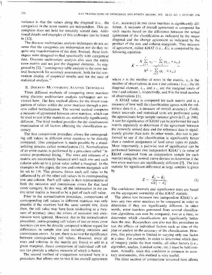
"I
170 IEEE TRANSACTIONS ON GEOSCIENCE AND REMOTE SENSING. VOL. GE-24. NO. I. JANUARY 1986
N2- ~ (Xi + * X-J. J
i= 1
(i .e., accuracy) in two error matrices is significantly dif-ferent. A measure of overall agreement is computed foreach matrix based on the difference between the actualagreement of the classification as indicated by the majordiagonal and the change agreement as indicated by theproduct of the row and column marginals. This measureof agreement, called KHAT (i.e., K), is computed by thefollowing equation:
The confidence intervals and significance tests are basedon the asymptotic normality of the KHAT statistic.
The above test between two independent KHAT's al-lows any two error matrices to be compared in order todetermine if they are significantly different. In otherwords, error matrices generated from several classifica-tion algorithms can now be compared, two at a time, todetermine which classifications are significantly betterthan the rest. Researchers can also use this procedure totest the effects of individual factors such as time of theyear or analyst on the accuracy of the classification. How-ever, this procedure is limited to varying only one factorat a time. For example, in order to determine which dateof imagery yields the best results, all other factors (i.e.,algorithm, analyst, Landsat scene, etc.) must be held con-stant. Actually, since this condition is common in accu-racy assessments, this method is very useful.
The third method of comparison reviewed here allows
(I)
where r is the number of rows in the matrix, Xii is thenumber of observations in row i and column i (i.e., the ithdiagonal element, Xi -J.. and X+ i are the marginal totals ofrow i and column i, respectively, and N is the total numberof observations 11].
A KHAT value is computed for each matrix and is ameasure of how well the classification agrees with the ref-erence data (i.e., a measure of overall accuracy). Confi-dence intervals and statistical tests are pertcJfmed usingthe approximate large sample variance given in [1, p. 396].A test for significance of KHAT can be performed for eachmatrix separately to determine if the agreement betweenthe remotely sensed data and the reference data is signif-icantly greater than zero. In other words, this test is per-formed to see if the classification is significantly betterthan a random assignment of land cover types to pixels.More importantly, a pairwise test of significance can beperformed between two independent KHAT's (a value ofKHAT computed from an independent sample for eachmatrix) using the normal curve deviate to determine if thetwo error matrices are significantly different 13]. The teststatistic for significant difference in large samples is givenby
N ~ XiiK = i=1
variance is that the values along the diagonal (i.e., thecategories) in the error matrix are independent. This as-sumption does not hold for remotely sensed data. Addi-tional details and examples of this technique can be foundin 1121.
The discrete multivariate analysis techniques do not as-sume that the categories are independent nor do they re-quire any transformation of the data. Instead, these tech-niques were designed to deal specifically with categoricaldata. Discrete multivariate analysis also uses the entireerror matrix and not just the diagonal elements. As sug-gested by [2), "contingency table analysis is the most nat-ural framework for accuracy assessment, both for the con-venient display of empirical results and for the ease ofstatistical analysis. "
II. DISCRETE MULTIVARIATE ANALYSIS TECHNIQUES
Three different methods of comparing error matricesusing discrete multivariate analysis techniques are re-viewed here. The first method allows for the direct com-parison of values within the error matrices through a pro-cess called normalization. The second method computesa measure of agreement between error matrices, which canbe used to test if the matrices are statistically significantlydifferent. The third method provides for the simultaneousexamination of all factors affecting the classification ac-curacy.
The first comparison procedure allows for correspond-ing cell values in different error matrices to be directlycompared. This comparison is made possible by a stand-ardizing process called normalization [1]. Normalizationof an error matrix is performed by a procedure called "it-erative proportional fitting." The rows and columns of amatrix are successively balanced until each row and eachcolumn adds up to a given value called a marginal. In theexamples in this paper, the row and column marginals willbe set to 1.0. This process forces each cell value to beinfluenced by all the other cell values in its correspondingrow and column. Each cell value is then representative ofboth the omission and commission errors for that landcover category. In this way, all the information in the en-tire error matrix is forced to be a part of each cell value.
Prior to the normalization procedure, comparisons ofcorresponding cell values in different matrices was onlypossible if the matrices had the same sample size. Eventhen, the cell value may have been misleading as a mea-sure of accuracy since the errors of omission and com-mission were ignored. However, due to the normalizationprocedure, corresponding cell values of two or more errormatrices can now be directly compared without regard fordifferences in sample size and including omission andcommission errors. As yet, there is no test for significancebetween corresponding cell values. However, since allrows and columns in the matrix are forced to add to agiven marginal, direct comparison of individual cell val-ues can provide a relative measure of which is better.
The second method of comparison reviewed here is aprocedure that allows one to test if the overall agreement

CONGALTON AND MEAD: REVIEW OF DISCRETE MULTIVARIATE ANALYSIS TECHNIQUES 171
one to simultaneously analyze more than a single factoraffecting the classification accuracy. This procedure is themost complicated of the three and is based on the log-linear model approach as described by [I], [6]. In thismethod, many variables (factors) affecting the accuracyand their interactions can be tested together to determinewhich are necessary (i.e., significant) in fully explainingthe classification accuracy.
In this method, the simplest model (combination of var-iables and their interactions) that provides a good fit to thedata (error matrices) is chosen using a model selectionprocedure. This procedure, which is similar to model se-lection procedures used in regression (i.e., forward selec-tion, etc.), allows the user to systematically search all pos-sible combinations of variables and their interactions andchoose the simplest combination that provides a good fitto the data. First, all uniform order log-linear models (i.e.,models with all possible n-way interactions, where n = Ito the number of variables) are examined and the simplestgood fit model is chosen. Each interaction of the chosenuniform order log-linear model is then tested for signifi-cance. If the interaction is not significant, it is droppedfrom the model. The process continues for each interac-tion until a model is found in which all the variables andtheir interactions are significant. For more details on thismodel selection procedure, see [6, Section 5.3]. The cri-teria used for determining the significance of the variablesand interactions in a model is based on the likelihood ratioC2 and the corresponding degrees of freedom for thatmodel.
This procedure uses a method of successive approxi-mations (i.e., "iterative proportional fitting") which con-verges to the maximum likelihood estimates of the mini-mum sufficient statistics as defined by the model. In otherwords, the "iterative proportional fitting" procedure at-tempts to fit the model of interest to the data. This pro-cedure is tedious and complicated and is almost alwaysdone on the computer. The likelihood ration C2 is thenused as a measure of "goodness of fit" of the model tothe data. The likelihood ratio statistic is used in place ofthe Pearson chi-square statistic because C2 can be parti-tioned, as is necessary in the model selection procedure,and still retain an approximate chi-square distributionwhile Pearson's statistic cannot. Therefore, the criticalvalue for testing if the model of interest is a good fit canbe obtained from a chi-square table with the appropriatedegrees of freedom [I], [6].
The log-linear model approach, unlike the KHAT sta-tistic, allows for the analysis of multi-way error matriceswith many factors. For example, error matrices generatedusing different dates, different algorithms, and differentanalysts all of the same scene of imagery, can be put to-gether and the factors significant in explaining the classi-fication accuracy identified. A possible practical result ofsuch an analysis could be that the image date is insignifi-cant, and therefore the imagery with the highest quality,irregardless of the date obtained, could be used in thestudy.
It should be realized here that performing any of thesethree comparison methods by hand is a very tedious pro-cess. Computer programs have been written to implementall three techniques and are available from the author. Thefirst and second procedures are very easy to use while thethird is somewhat more complicated.
III. EXAMPLE ANALYSES
Data used to demonstrate the normalization procedureand the test of agreement procedure were part of a studydone on various image processing software packages bythe U.S. Army Engineer Waterways Experiment StationEnvironmental Laboratory [11]. Each software packagewas used to produce the best possible classification 0 theSimeon Southeast USGS 7~-min quadrangle into threegeneral land cover categories: water (WA), wetlands(WE), and nonwetlands (NW). The three software pack-ages evaluated were: the EDITOR software developed atNASA Ames Research Center, the GISS software devel-oped at the Goddard Institute for Space Sciences, and theVICAR software developed at Washington State Univer-sity. The original and normalized error matrices for eachof the three software packages are given in Tables I-III.Table IV presents a comparison between the overall per-formance accuracy, the measure of agreement (KHAT),and the normalized performance accuracy for the threesoftware packages. Normalized performance accuracy iscomputed in the same way as overall performance accu-racy except on the normalized matrix. This measure ofaccuracy differs from the overall performance accuracy inthat the cell values along the major diagonal in the nor-malized matrix now incorporate the omission and com-mission error in the matrix as a result of the "iterativeproportional fitting" procedure. Note that in this case allthree measures of accuracy yield the same ranking (bestto worst). However, because these are three differentmeasures of accuracy and contain different levels of infor-mation, they do not always have to yield the same ranking.
As previously mentioned, normalization allows for thedirect comparison of corresponding cell values in each ofthe three matrices. For example, Table V contains the per-cent correct and normalized values for the water categoryin each matrix. In the percent correct calculation only er-rors of omission are accounted for. However, the normal-ized value considers both errors of omission and commis-sion as well as negating the effect of sample size. The resultof considering both omission and commission errors in theaccuracy measure is clearly demonstrated by comparingthe values in the water category for the EDITOR softwareand the VICAR software (Table V). Notice that the EDI-TOR software has a percent correct for the water categoryof 71 percent and a normalized value of 0.8729 while theVICAR software has a much higher percent correct of 81percent and yet a normalized value of 0.8630. This appar-ent discrepancy in results is mostly due to the large com-mission error (placing 4184 wetland pixels in the watercategory) in the VICAR error matrix (see Table III). The
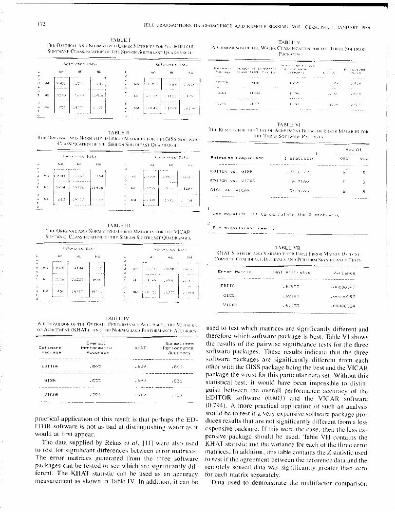
172 IEEE TRANSACTIONS ON GEOSCIENCE AND RH:I0TE SENSING, VOL, GE-24, NO, I, JANUARY Ino
TABLE I
THE ORIGI~AL A'I1l NORMALIZEIl ERROR MAl RICES FORTHE EDITOR
SOfTWARE CLASSII'ICATIO~ OF THE SIMEO~ SOU HF:\ST QI.JAIlRA~(ill'
TABLE V
A COMPAIHSO'l 01' I'HE W.·\lI'R CLASSIFICATION H)R 1'111.TIIRI-I SOil WARI'
PACKA"I'.S
WA
ReferenLE' Data
WE Nth WA WE NWSf:d tw~r
F'<" I: l, .'=Is!C' I~ J0-1 Cu, r £:'c~~l \(
fllO·'i F']1 ::.ed
{DlHW
'.'ll
'h,131
TABLE II
TilE OIWilNAL ,\NIl NOHM,\IIZI'f) EHHOH MAJJ{ICI:S HlR Till' GISS SOFTWARI-
Ci;\SSII-ICATIO~ 01' 1'111-SIMEON SOUTIIFAST QLAIlR.\Mill'~~~~-------
TABLE VI
'1'111'.RLSlilTS F"R 1111.TISI 01· A(;RFI\1I·.', I BI'TWITN ERR"" MAl Rlll.S HJR
1111,.TIIRI'I'. S""I WARI: P,""NiiS_._~-~---~_._-~--~-~_._~-~------~------- ----.-----.--------
ResultPalrwiS8 ComparIson
1Z StatIstIC 95:. 901..
W'::', WI
USE' equatIon (1) to calculate the Z stdtlstlC
EDITOR vs. GIS!::, s
5
5
s
5
5
6.716U'yICAf:;;
GISS Y5. VICAr,:
EDITOR
W'::i Wt NW
d W(-'t 11)84 16,l
wE 17'-14 ] I 4 ~,6
J)d l\il>; 6t~,:::-. 1O~:~~7
TABLE III
1'111'ORll>INAL ,\NIl NORMAII/I'.1l ERROI{ MAl RICES HJR Till· VICAR
SOFTWARECLASSII'ICArION 01, rill' SIMEON SOUTIILAST QUAIlRAMil.l'
5 sIgnifIcant resLIJt
KHAT StatIstIC Var-iance
GISS
EDITOR
Err-ot'" Matr i;<
TABLE VII
KHAT SIATISTIC ,\ND V'\RIA~CI' F"R EAlli ERROR MATRIX l!SLIJ TO
COMPUTL CONIIDL'IC'!. I~TLRV,\LS ,\NIJ PLRH)RM Slli~IHCANCT TESTS----_.~------~----~~-_._---._--_.~--~
WL
'-
D
a-- --- --"'~----
898('
41 E;II
W':i ~JE NW
'JICAR .61155 .00000::-·54
TABLE IV
A COMPARISON 01' Till' OVIRALL PFRHJRMANlT Al'CURACY, TIll. MF.\SURL
or' AGREEMENT (KHAT), ANIl Till' NORMAII/.l:Il PERI'OI{MANCF AlTURAC\
practical application of this result is that perhaps the ED-ITOR software is not as bad at distinguishing water as itwould at fi rst appear.
The data supplied by Rekas cf al. III] were also usedto test for significant differences between error matrices.The error matrices generated from the three softwarepackages can be tested to see which are significantly dif-ferent. The KHAT statistic can be used as an accuracymeasurement as shown in Table IV. In addition, it can be
SoftwarePackage
EDITOR
GISS
VICAR
OverallPerformance
Accuracy
.803
.833
.794
f:HAT
.629
.692
.612
Nor-mall zedPerformance
Accur"acy
.836
.789
used to test which matrices are significantly different andtherefore which software package is best. Table VI showsthe results of the pairwise significance tests for the threesoftware packages, These results indicate that the threesoftware packages are significantly different from eachother with the GISS package being the best and the VICARpackage the worst for this particular data set. Without thisstatistical test, it would have been impossible to distin-guish between the overall performance accuracy of theEDITOR software (0.803) and the VICAR software(0.794). A more practical appl ication of such an analysiswould be to test if a very expensive software package pro-duces results that are not significantly different from a lessexpensive package. If this were the case, then the less ex-pensive package should be used. Table VII contains theKHAT statistic and the variance for each of the three errormatrices. In addition, this table contains the Z statistic usedto test if the agreement between the reference data and theremotely sensed data was significantly greater than zerofor each matrix separately.
Data used to demonstrate the multi factor comparison

CONGALTON AND MEAD: REVIEW OF DISCRETE MULTIVARIATE ANALYSIS TECHNIQUES 173
TABLE VIIITHE UKIFORM ORDER MODELS H1R THE FOLR-WAY TABLE COMPARING
ENHANCEMENT TECH:-JI()LES AND CLASSIFICATIO:-J ALGORITHMS
TABLE IXTHE MODEL SELECTION PROCESS FOR THE FOUR-WAY TABLE COMPARING
EKHAKCE\1EKT TECHNIQUES AND CLASSIFICATION ALGORITHMS
MUD!::!. df RESULT df Bt:;~UL'I'
--~-- 112I1lJII1I'1I2)H ,4J 10"/32.65712 )15 puor fi t
[1211['1I'41121I1'J"1 2)0.22101, 2")-- -- ----- ----- ----- 1----112111)1I141124I1Y'}S 1"7.8)2,,6 2/"
11][<]13]['1} 10fHl8.t1·/281. • ._u _
1\112)[ 1,)[ 11,][ <3][ 2/111JIIJ 145.86"28
15< 1'00/' fit
""" ""ud 1 i l---------- ..----- - --.-
22'1.51772 24)
I?oud Ii l
,guod fi l
,.·ood ri l
156.5)1 )[ guo.1 fit
20.<,10')1'1 good ljl}116. Ol~ol.t 2)5 ,-'oDd fj t
mQ[jtd t.: Leu t aud ~uoJ fi t C!illuS8 D
G2(1i:) _ G2(lJ) -.,. "/] .tll'Jj) .•.•)cl<jdr aitlnlficallt [;0
clm' t t\rul' { 11l}
1 l'JlI"'JP"J 1Oln. 9?U76 )25 poor fi t
-. -~_. ---_.-~-~- -- -------_. ------ ------
I IlJll"lI 1/'11 2 I .c)1 .II )ld:l5 25'j p:ood fi t------------- ------ ---- .----
I ' '1H"'lI "IJ ~29.S210H 25) p,ood flt
------------[ ," II"" II "I] D I SU.66500 25'1 f'(Jul1 fil
~.u{Jd fi t
puor fi t
I!;ood fi t
nut l:Jig'lificalltso lirup (1 3}.
262
not tdglli ficant sudl'0p I 12]
flOt ::dgllificBlll l;O
dl'op [2)1
242.096116
Illu.lul [J Le::ll llnd gu{,d 1\ t
(~"IIJ) - U2(';1 ~ IU./'c16<:-X\df
IlIlldel C best Slid ,"ood fi t
G21';) _ U2(B) .0.1709195-X;dr
I 21'11'411' ] E
IllUdul Ii lJt;!:..;t alllJ good fit
1.;2(11) ~ l;(:(A) :0. 2.1J6tnf.} x~(H
11211' )lI"'lI 24 J 107J). 027~ )21~ poor fit
r 12)[I)JI1411 )41 2)1.)918 252 gool! fU----
[12l! [)lI2"lI J'I) 229./1002 252 ~ood fi l
[ 1211'" 1I ,I'll JlIj 15tl,'I')I.1 252 guod rit---- . .---
(I) 1I I" II 21'lI )4 J C 11ll:Lou,lf 25? ~ood fi L
_.__ ._--~-- ~--- - ~~-- -_._~
good fit model to the data. Table IX shows the steps of thisprocess. The next step in the model selection process thenis to eliminate a two-way interaction term from the two-way unitorm order model. By eliminating one two-wayterm, six new models result, each with a different com-bination of the five remaining two-way interaction terms.These six new models are tested for "goodness of fit"based on the G2 and the appropriate degrees of freedom(df), and model B is chosen to be the simplest good fitmodel. The eliminated two-way interaction term is testedfor significance by comparing the fit of the two-way uni-form order model, labeled A in Table VIII, with model B.This test is possible because partitioning G2 still results
procedure were supplied by Gregg et al. [7]. These datawere collected as part of an operational study of Landsatimagery for inventory purposes in the State of Washing-ton. In this example, two classification algorithms, twoenhancement techniques, 10 reference data categories, and10 Landsat data categories were studied resulting in a four-way table of dimensions 2 by 2 by 10 by 10. Unfortunately,due to the size of this tour-way table, it cannot be printedhere. However, the original data can be tound in the papercited above.
As previously described, a model selection procedurewas used to determine the simplest good fit model to thedata. Table VIII contains the unitorm order log-linearmodels for these data. Notice that, because this is a four-way table, the unitorm order models consist of the modelswith all three-way, all two-way, and all one-way interac-tions. The unitorm order model of all four-way interac-tions (written as [1 2 3 4]) is the complete or saturatedmodel and will always fit the data because it contains allthe factors and their interactions. However, the object hereis to eliminate the nonsignificant factors or interactionsand find the simplest good fit model.
In this example, classification algorithm (denoted vari-able [1]), enhancement technique (denoted variable [2]),and the reference data (denoted variable [31) are calledexplanatory variables while the Landsat data (denoted var-iable [4]) is called the response variable. This terminologyis derived from the idea that the first three variables arebeing used to try to explain the response (i .e., the Landsatclassification). The interaction terms in the model are rep-resented as combinations of these variables enclosed inbrackets (e.g., [12] is the interaction between algorithmand enhancement).
Table VIII shows that the two-way interaction unitormorder log-linear model is the simplest good fit model asdetermined by the likelihood ratio G2
• The one-way uni-form order model is a poor fit while the three-way unitormorder model is a good fit, but is more complicated thanthe two-way model. Notice that the two-way uniform ordermodel consists of six two-way interaction terms. The ob-ject then is to systematically eliminate all the nonsignifi-cant factors or their interactions leaving just the simplest
174IEEE TRANSACTIONS ON GEOSCIENCE AND REMOTE SENSING, VOL. GE-24, NO, !, JANUARY 1986
in a chi-square distribution. Because this test is not sig-nificant, the [23] interaction term can be dropped fromthe model (see Table IX).
This same process is then repeated on model B by elim-inating another two-way interaction term and testing theresulting five models. The results of the test yield modelC as the simplest good fit model. Also, the test shows the[12] interaction term to be not significant; therefore, it isdropped from the model. The process is repeated again,leading to model D and the elimination of the [/3] inter-action. Note that one of the possible models tested herecontained a one-way interaction term. The process is re-peated one last time, resulting in model E as the simplestgood fit model. However, the test between models D andE was significant; therefore the [14] interaction cannot beeliminated from the model without losing some of the crit-ical information about the data. Therefore, model D [/41[24] [34]) is selected as the simplest good fit model to thedata.
Model D indicates that there are no three-way interac-tions necessary to explain the data. Instead, there is acombined effect due to each explanatory variable (i.e., al-gorithm, enhancement, and reference data) separately withthe response. In other words, for this example each factorcontributes significantly to the performance of classifyingthe image and, therefore, none can be eliminated.
IV. SUMMARY AND CONCLUSIONS
The three discrete multivariate analysis techniques re-viewed here are very helpful in assessing the accuracy ofclassifications derived from remotely sensed data. Thesetechniques have the advantage of allowing the user toquantitatively compare the different aspects of the classi-fication process and assess the results. In addition, eachtechnique is easily implemented by a computer program.However, the results of these quantitative techniques areonly as good as the error matrices used in the computa-tions. A great deal more research is needed in the sam-pling aspects of accuracy assessment to insure that the er-ror matrices are indeed representative of the entire areaclassified using the remotely sensed data.
REFERENCES
II] Y. Bishop, S, Fienberg, and P, Holland, Discrete Multivariate Anal-ysis-Theory and Practice. Cambridge, MA: MIT Press, 1975,
[2] D. Card, "Using known map category marginal frequencics to im-prove estimates of thematic map accuracy," Photogrammetr, En[;..vol. 48, no. 3, pp, 431-439. 1982.
[3J J. Cohen, "A coefficient of agreement f())' nominal scalcs," Educa-tion. Psych. Measurement, vol. XX, no, I, pp. 37-40. 1960,
[41 R, Congalton, "Thc use of discrete multivariate analysis techniquesf(lr the assessment of Landsat classification accuracy." M.S, thesis,Virginia Poly tech. lnst. and State Univ., 1981.
15] R. Congalton, R. Oderwald, and R, Mead, "Assessing Landsat clas-sification accuracy using discrete multivariate analysis statistical tech-niques," Photogrammetr. Eng., vol. 49. no, 12, pp. 1671-1678, 1983.
161 S. Fienberg, The Analysi.I' o{ Cros.I-Classified CateRl/rical Data.Cambridge, MA: MIT Prcss, 1980.
[7] T, Gregg, E. Barthmaier, R. Aulds, and R. Scott. "Landsat opera-tional inventory study," Div. Tech, Serv .. State of Washington, Dep.Nat. Res., Olympia. WA, 1979.
18] R. Hoffer, "Natural resource mapping in mountainous terrain hy com-puter analysis of ERTS-I satellite data," LARS Res. Ball. 919, PurdueUniv .. 1975.
19] R. Hoffer and M, Fleming, "Mapping vegetative cover by computeraided analysis of satellite data." LARS 71'cl1. Ref'. 011178. PurdueUniv., 1978.
110] R. Mead and M. Meyer, "Landsat digital data application to I()restvegetation and land use classification in Minnesota," in Proc. Mach.Process. Remotely Sensed Data (Purdue Univ.), pp, 270-280. 1977.
[111 A. Rekas, J. Stoll, and H. Struve, "An evaluation of Landsat classi-fication procedures t(lr wetlands mapping," Tech. Rep. EL-84-(inpress). U.S, Army Waterways Experiment Station, Vickshurg, MS,1984.
[12] G, Rosenfield. "Analyzing thematic maps and mapping for accu-racy, "U.S. Gco. Survey Opcn File Rep. 82-239. 1982.
[13] G. Snedecor and W. Cochran, Statistical Methods, 6th cd. Ames,IA: Iowa State Press, 1976.
[14] M. Hord and W. Brooner, "Land-use map accuracy criteria," Pho-tOI;:rammetr. En[;., vol. 42, no. 5, pp. 67]-677, 1976.
[]5] J. van Genderen and B. Lock, "Testing land use map accuracy," Pho-togrammetr. Eng., vol. 43, no. 9, pp. 1135-1137, 1977.
[161 S. Aronoff', "Classification accuracy: A user approach," Photogram-metro Eng., vol. 48, no. 8, pp. 1299-1307, 1982.
*
Russell C. Congalton received the B.S. degree in t()restry from RutgersUniversity in 1979 and the M.S, and Ph.D. degrees in I(lrest biometrics andremote sensing from Virginia Polytechnic Institute and State University in1981 and 1984, respectively.
He spent 1985 as a post-doctorate researcher f(lr the Remote SensingGroup of the Environmental Laboratory at the U.S. Army Corps of Engi-neers Waterways Experiment Station. Presently, he is employed as an As-sistant Professor of Remote Sensing in the Department of Forestry and Re-source Management at the University of California, Berkeley,
*
Roy A. Mead received the B.S, degree in botany from Northern ArizonaState University, the M.S. degree in remotc sensing from Colorado StateUniversity, and the Ph. D, degree in remote sensing from the University ofMinnesota.
He has considerable experience in remote sensing and geographic inf()f-mation systems with govcrmncnt agencies. priVate industry, and academia.He is currently employed as a Geographic Information Systcms Specialistlor the U.S. Forest Service.
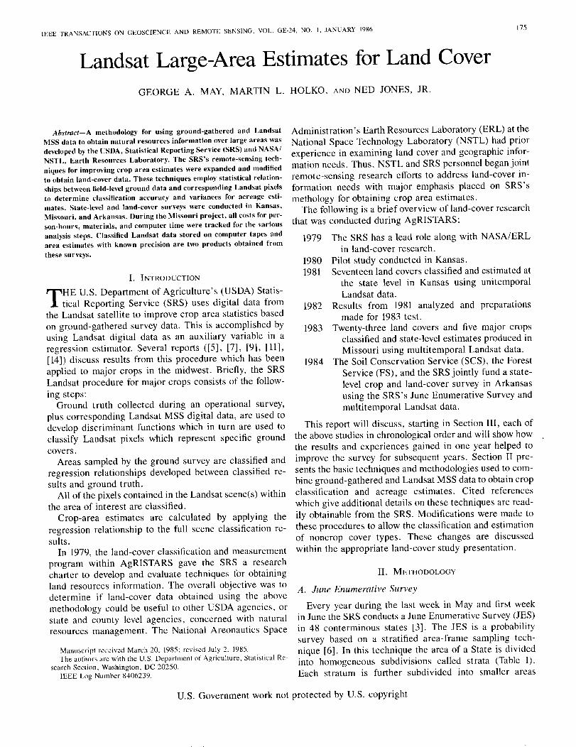
IEEE TRANSACTIONS ON GEOSCIENCE AND REMOTE SENSING, VOL. GE-24, NO. I, JANUARY 1986
Landsat Large-Area Estimates for Land CoverGEORGE A. MAY, MARTIN L. HaLKO, AND NED JONES, JR.
175
Abstract-A methodology for using ground-gathered and LandsatMSS data to obtain natural resources information over large areas wasdeveloped by the USDA, Statistical Reporting Service (SRS) and NASA/NSTL, Earth Resources Laboratory. The SRS's remote-sensing tech-niques for improving crop area estimates were expanded and modifiedto obtain land-cover data. These techniques employ statistical relation-ships between field-level ground data and corresponding Landsat pixelsto determine classification accuracy and variances for acreage esti-mates. State-level and land-cover surveys were conducted in Kansas,:\1issouri, and Arkansas. During the Missouri project, all costs for per-son-hours, materials, and computer time were tracked for the variousanalysis steps. Classified Landsat data stored on computer tapes andarea estimates with known precision are two products obtained fromthese surveys.
I. INTRODUCTION
THE u.s. Department of Agriculture's (USDA) Statis-tical Reporting Service (SRS) uses digital data from
the Landsat satellite to improve crop-area statistics basedon ground-gathered survey data. This is accomplished byusing Landsat digital data as an auxiliary variable in aregression estimator. Several reports ([5], [7], [9], [11],[14]) discuss results from this procedure which has beenapplied to major crops in the midwest. Briefly, the SRSLandsat procedure for major crops consists of the follow-ing steps:
Ground truth collected during an operational survey,plus corresponding Landsat MSS digital data, are used todevelop discriminant functions which in turn are used toclassify Landsat pixels which represent specific groundcovers.
Areas sampled by the ground survey are classified andregression relationships developed between classified re-sults and ground truth.
All of the pixels contained in the Landsat scene(s) withinthe area of interest are classified.
Crop-area estimates are calculated by applying theregression relationship to the full scene classification re-sults.
In 1979, the land-cover classification and measurementprogram within AgRISTARS gave the SRS a researchcharter to develop and evaluate techniques for obtainingland resources information. The overall objective was todetermine if land-cover data obtained using the abovemethodology could be useful to other USDA agencies, orstate and county level agencies, concerned with naturalresources management. The National Areonautics Space
Manuscript received March 20, 1985; revised July 2. 1985.The authors are with the U.S. Department of Agriculture, Statistical Re-
search Section, Washington, DC 20250.IEEE Log Number 8406239.
Administration's Earth Resources Laboratory (ERL) at theNational Space Technology Laboratory (NSTL) had priorexperience in examining land cover and geographic infor-mation needs. Thus, NSTL and SRS personnel began jointremote-sensing research efforts to address land-cover in-formation needs with major emphasis placed on SRS'smethology for obtaining crop area estimates.
The following is a brief overview of land-cover researchthat was conducted during AgRISTARS:
1979 The SRS has a lead role along with NASA/ERLin land-cover research.
1980 Pilot study conducted in Kansas.1981 Seventeen land covers classified and estimated at
the state level in Kansas using unitemporalLandsat data.
1982 Results from 1981 analyzed and preparationsmade for 1983 test.
1983 Twenty-three land covers and five major cropsclassified and state-level estimates produced inMissouri using multitemporal Landsat data.
1984 The Soil Conservation Service (SCS), the ForestService (FS), and the SRS jointly fund a state-level crop and land-cover survey in Arkansasusing the SRS's June Enumerative Survey andmultitemporal Landsat data.
This report will discuss, starting in Section III, each ofthe above studies in chronological order and will show howthe results and experiences gained in one year helped toimprove the survey for subsequent years. Section II pre-sents the basic techniques and methodologies used to com-bine ground-gathered and Landsat MSS data to obtain cropclassification and acreage estimates. Cited referenceswhich give additional details on these techniques are read-ily obtainable from the SRS. Modifications were made tothese procedures to allow the classification and estimationof noncrop cover types. These changes are discussedwithin the appropriate land-cover study presentation.
II. METHODOLOGY
A. June Enumerative Survey
Every year during the last week in May and first weekin June the SRS conducts a June Enumerative Survey (JES)in 48 conterminous states [3]. The JES is a probabilitysurvey based on a stratified area-frame sampling tech-nique [6]. In this technique the area of a State is dividedinto homogeneous subdivisions called strata (Table I).Each stratum is further subdivided into smaller areas
U.S. Government work not protected by U.S. copyright
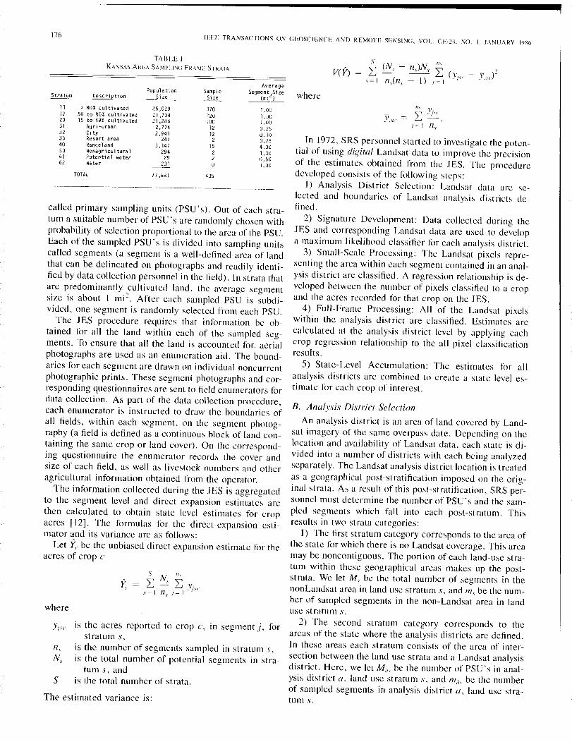
176IEEE TRANSACTIONS ON GEOSCIENCE AND REMOTE SENSING, VOL, Gf'-24, NO. L JANUARY 19R6
In 1972, SRS personnel started to investigate the poten-tial of using dixital Landsat data to improve the precisionof the estimates obtained from the JES. The proceduredeveloped consists of the following steps:
I) Analysis District Selection: Landsat data are se-lected and boundaries of Landsat analysis districts de-fined.
2) Signature Development: Data collected during theJES and corresponding Landsat data are used to developa maximum likelihood classifier for each analysis district.
3) Small-Scale Processing: The Landsat pixels repre-senting the area within each segment contained in an anal-ysis district arc classified. A regression relationship is de-veloped between the number of pixels classified to a cropand the acres recorded for that crop on the JES.
4) Full-Frame Processing: All of the Landsat pixelswithin the analysis district are classified. Estimates arecalculated at the analysis district level by applying eachcrop regression relationship to the all-pixel classificationresults.
5) State-Level Accumulation: The estimates for allanalysis districts are combined to create a state level es-timate for each crop of interest.
B. Analysis District Selection
An analysis district is an area of land covered by Land-sat imagery of the same overpass date. Depending on thelocation and availability of Landsat data, each state is di-vided into a number of districts with each being analyzedseparately. The Landsat analysis district location is treatedas a geographical post-stratification imposed on the orig-inal strata. As a result of this post-stratification, SRS pe~-sonnel must determine the number of PSU's and the sam-pled segments which fall into each post-stratum. Thisresults in two strata categories:
I) The first stratum category corresponds to the area ofthe state for which there is no Landsat coverage. This areamay be noncontiguous. The portion of each land-use stra-tum within these geographical areas makes up the post-strata. We let M, be the total number of segments in thenonLandsat area in land use stratum .1', and tn, be the num-ber of sampled segments in the non-Landsat area in landuse stratum s.
2) The second stratum category corresponds to theareas of the state where the analysis districts are defined.In these areas each stratum consists of the area of inter-section between the land use strata and a Landsat analysisdistrict. Here, we let Ma., be the number of PSU's in anal-ysis district a, land use stratum s, and m,is be the numberof sampled segments in analysis district a, land use stra-tum s.
s (N II.,L; s - fl.JN, 2: - .7
( I) (Yi" - 'vser,~I fl.,fl.,. - ,~I
TABLE IKA\JSAS AREA SA.vIPLlN(; FRA\1E STRATA
AverageStratum
Population Samp 1e Segment2S 1zeDescription Sf ze _ Sf ze __ lm_1_l _
11 ) 80X cultivated 25,028 170 LOa12 50 to 80% cultivated 21,704 120 LOa20 15 to 49% cultivated 21,286 100 LOa31 Agri-urban 2,774 12 0.2532 Ci ty 2,941 12 0,1033 Resort area 247 2 0.2540 Rangeland 3,147 15 4.0050 Nonagricultural 294 2 1.0061 Potential water 29 2 0.5062 Water 231 a 1.00
TOTAL 77 ,681 435
called primary sampling units (PSU's). Out of each stra-tum a suitable number of PSU's are randomly chosen withprobability of selection proportional to the area of the PSU.Each of the sampled PSU' s is divided into sampling unitscalled segments (a segment is a well-defined area of landthat can be delineated on photographs and readily identi-fied by data collection personnel in the field). In strata thatare predominantly cultivated land, the average segmentsize is about I mi2
. After each sampled PSU is subdi-vided, one segment is randomly selected from each PSU.
The JES procedure requires that information be ob-tained for all the land within each of the sampled seg-ments. To ensure that all the land is accounted for, aerialphotographs are used as an enumeration aid. The bound-aries for each segment are drawn on individual noncurrentphotographic prints. These segment photographs and cor-responding questionnaires are sent to field enumerators fordata collection. As part of the data collection procedure,each enumerator is instructed to draw the boundaries ofall fields, within each segment, on the segment photog-raphy (a field is defined as a continuous block of land con-taining the same crop or land cover). On the correspond-ing questionnaire the enumerator records the cover andsize of each field, as well as livestock numbers and otheragricultural information obtained from the operator.
The information collected during the JES is aggregatedto the segment level and direct expansion estimates arethen calculated to obtain state level estimates for cropacres [12]. The formulas for the direct-expansion esti-mator and its variance are as follows:
Let Yc be the unbiased direct expansion estimate for theacres of crop c
S N II,"" s",~~6 Yil"
I'~ I fl.,.1~ I
where
YIIC is the acres reported to crop c, in segment j, forstratum s,
fl., is the number of segments sampled in stratum s,N, is the total number of potential segments in stra-
tum S, andS is the total number of strata.
The estimated variance is:
where
v(h
v00/ .s!'
III "
== 2: ~~.i I fl.,
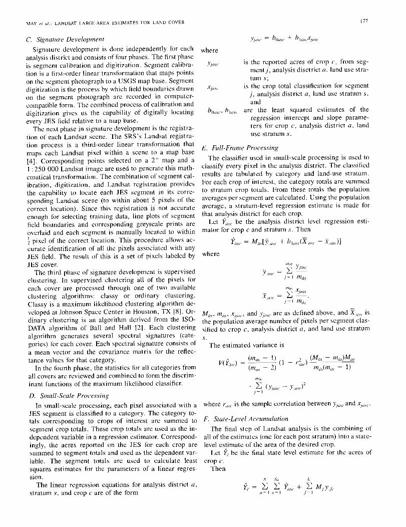
MAY el al.: LANDSAT LARGE-AREA ESTIMATES FOR LAND COVER 177
where
where
where rase is the sample correlation between Yjalc and Xja,\c'
A Sd L
Y,.. ~ ~ Y,ise + ~ Mry!ca=1 '\=1 f= I
F. State-Level AccumulationThe final step of Landsat analysis is the combining of
all of the estimates (one for each post stratum) into a state-level estimate of the area of the desired crop.
Let Y,. be the final state level estimate for the acres ofcrop c.
Then
A (md.l· - 1) (IV( ~lsC) == ----
(m"" - 2)
Mil'" m,h" Xjasco and )liase are as defined above, and Xasc isthe population average number of pixels per segment clas-sified to crop c, analysis district a, and land use stratums.
The estimated variance is
E. Full-Frame ProcessingThe classifier used in small-scale processing is used to
classify every pixel in the analysis district. The classifiedresults are tabulated by category and land-use stratum.For each crop of interest, the category totals are summedto stratum crop totals. From these totals the populationaverages per segment are calculated. Using the populationaverage, a stratum-level regression estimate is made forthat analysis district for each crop.
Let Yilse be the analysis district level regression esti-mator for crop c and stratum s. Then
Yilse = Mils[Y.ase + blasix.ase - x.a.H·)]
Yia.IT boase + blascxiasc
Yjasc is the reported acres of crop c, from seg-ment}, analysis disctrict a, land use stra-tum s;
Xja.le is the crop total classification for segment}, analysis district a, land use stratum s,and
bom,., blase are the least squared estimates of theregression intercept and slope parame-ters for crop c, analysis dist rict a, landuse stratum s.
nld,\ X.== ~ Jase •
X.asc LJj= I mils
milS y.== ~ .lase
Y.ase ~j= 1 mils
C. Signature DevelopmentSignature development is done independently for each
analysis district and consists of four phases. The first phaseis segment calibration and digitization. Segment calibra-tion is a first-order linear transformation that maps pointson the segment photograph to a USGS map base. Segmentdigitization is the process by which field boundaries drawnon the segment photograph are recorded in computer-compatible form. The combined process of calibration anddigitization gives us the capability of digitally locatingevery JES field relative to a map base.
The next phase in signature development is the registra-tion of each Landsat scene. The SRS' s Landsat registra-tion process is a third-order linear transformation thatmaps each Landsat pixel within a scene to a map base[4]. Corresponding points selected on a 20 map and a1 :250 000 Landsat image are used to generate this math-ematical transformation. The combination of segment cal-ibration, digitization, and Landsat registration providesthe capability to locate each JES segment in its corre-sponding Landsat scene (to within about 5 pixels of thecorrect location). Since this registration is not accurateenough for selecting training data, line plots of segmentfield boundaries and corresponding greyscale prints areoverlaid and each segment is manually located to within~ pixel of the correct location. This procedure allows ac-curate fdentification of all the pixels associated with anyJES field. The result of this is a set of pixels labeled byJES cover.
The third phase of signature development is supervisedclustering. In supervised clustering all of the pixels foreach cover are processed through one of two availableclustering algorithms: classy or ordinary clustering.Classy is a maximum likelihood clustering algorithm de-veloped at Johnson Space Center in Houston, TX [8]. Or-dinary clustering is an algorithm derived from the ISO-DATA algorithm of Ball and Hall [2]. Each clusteringalgorithm generates several spectral signatures (cate-gories) for each cover. Each spectral signature consists ofa mean vector and the covariance matrix for the reflec-tance values for that category.
In the fourth phase, the statistics for all categories fromall covers are reviewed and combined to form the discrim-inant functions of the maximum likelihood classifier.
D. Small-Scale ProcessingIn small-scale processing, each pixel associated with a
JES segment is classified to a category. The category to-tals corresponding to crops of interest are summed tosegment crop totals. These crop totals are used as the in-dependent variable in a regression estimator. Correspond-ingly, the acres reported on the JES for each crop aresummed to segment totals and used as the dependent var-iable. The segment totals are used to calculate leastsquares estimates for the parameters of a linear regres-sion.
The linear regression equations for analysis district a,stratum s, and crop c are of the form
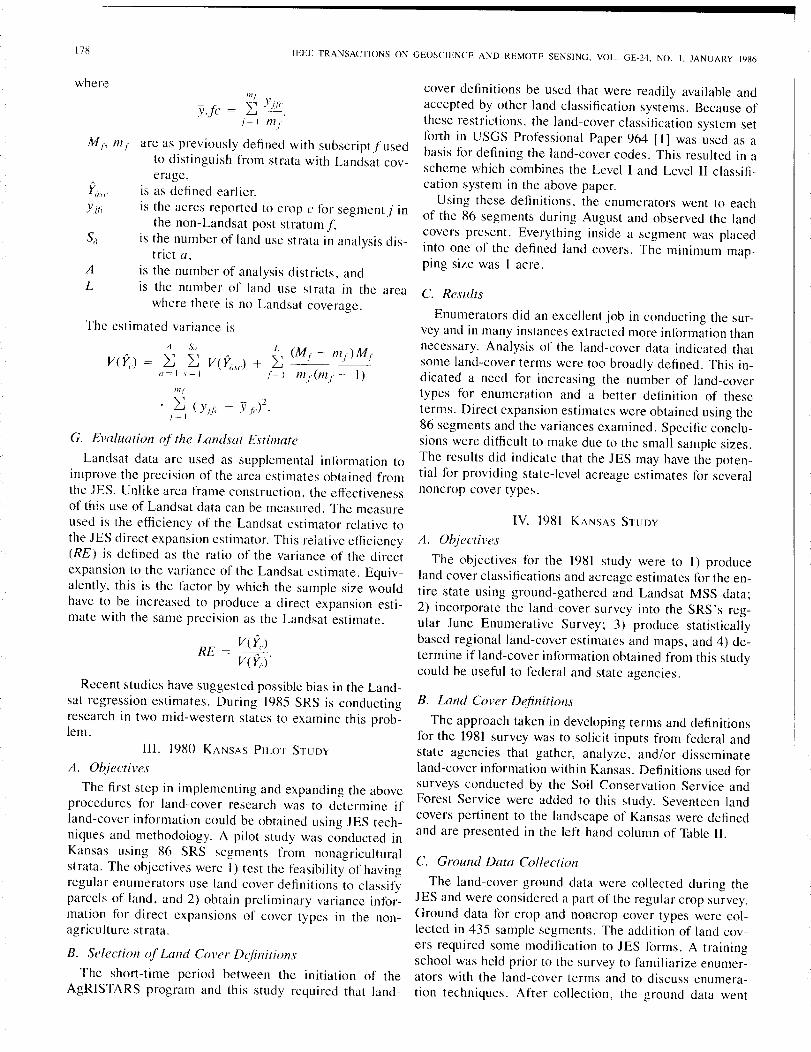
171;IEEE TRANSACTIONS ON GEOSCIENCE AND REMOTE SENSING. VOL. GE-24. NO. I. JANUARY 1986
where/lit
- ,,~ Y if,V.tc = u -'''-." j~ I tn,
Mr' tnj are as previously defined with subscript fusedto distinguish from strata with Landsat cov-erage,
r"s, is as defined earlier,Yjji is the acres reported to crop c for segmentj in
the non- Landsat post st ratum f,S" is the number of land use strata in analysis dis-
trict a,A is the number of analysis districts, andL is the number of land use strata in the area
where there is no Landsat coverage.
The estimated variance is
G. Evaluation of the Landsat EstimateLandsat data are used as supplemental information to
improve the precision of the area estimates obtained fromthe JES. Unlike area frame construction, the effectivenessof this use of Landsat data can be measured. The measureused is the efficiency of the Landsat estimator relative tothe JES direct expansion estimator. This relative efficiency(RE) is defined as the ratio of the variance of the directexpansion to the variance of the Landsat estimate. Equiv-alently, this is the factor by which the sample size wouldhave to be increased to produce a direct expansion esti-mate with the same precision as the Landsat estimate.
RE = !" (~) .V (1',)
Recent studies have suggested possible bias in the Land-sat regression estimates. During 1985 SRS is conductingresearch in two mid-western states to examine this prob-lem.
III. 1980 KANSAS PILOT STUDYA. Objectives
The first step in implementing and expanding the aboveprocedures for land-cover research was to determine ifland-cover information could be obtained using JES tech-niques and methodology. A pilot study was conducted inKansas using 86 SRS segments from nonagriculturalstrata. The objectives were I) test the feasibility of havingregular enumerators use land cover definitions to classifyparcels of land, and 2) obtain preliminary variance infor-mation for direct expansions of cover types in the non-agriculture strata.
B. Selection of Land Cover DefinitionsThe short-time period between the InItiatIOn of the
AgR1STARS program and this study required that land-
cover definitions be used that were readily available andaccepted by other land classification systems. Because ofthese restrictions, the land-cover classification system setforth in USGS Professional Paper 964 II] was used as abasis for defining the land-cover codes. This resulted in ascheme which combines the Level I and Level IIclassifi-cation system in the above paper.
Using these definitions, the enumerators went to eachof the 86 segments during August and observed the landcovers present. Everything inside a segment was placedinto one of the defined land covers. The minimum map-ping size was I acre.
C. ResultsEnumerators did an excellent job in conducting the sur-
vey and in many instances extracted more information thannecessary. Analysis of the land-cover data indicated thatsome land-cover terms were too broadly defined. This in-dicated a need for increasing the number of land-covertypes for enumeration and a better definition of theseterms. Direct expansion estimates were obtained using the86 segments and the variances examined. Specific conclu-sions were difficult to make due to the small sample sizes.The results did indicate that the JES may have the poten-tial for providing state-level acreage estimates for severalnoncrop cover types.
IV 1981 KANSAS STUDYA. Objectives
The objectives for the 1981 study were to I) produceland cover classifications and acreage estimates for the en-tire state using ground-gathered and Landsat MSS data;2) incorporate the land-cover survey into the SRS's reg-ular June Enumerative Survey; 3) produce statisticallybased regional land-cover estimates and maps, and 4) de-termine if land-cover information obtained from this studycould be useful to federal and state agencies.
B. Land Cover DefinitionsThe approach taken in developing terms and definitions
for the 1981 survey was to solicit inputs from federal andstate agencies that gather, analyze, and/or disseminateland-cover information within Kansas. Definitions used forsurveys conducted by the Soil Conservation Service andForest Service were added to this study. Seventeen landcovers pertinent to the landscape of Kansas were definedand are presented in the left-hand column of Table II.
C. Ground Data CollectionThe land-cover ground data were collected during the
JES and were considered a part of the regular crop survey.Ground data for crop and noncrop cover types were col-lected in 435 sample segments. The addition of land cov-ers required some modification to JES forms. A trainingschool was held prior to the survey to familiarize enumer-ators with the land-cover terms and to discuss enumera-tion techniques. After collection, the ground data went
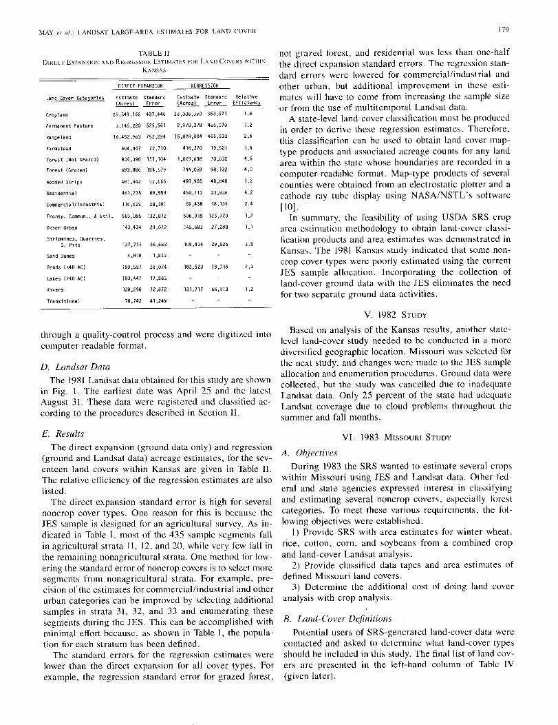
MAY el "I.: LANDSAT LARGE-AREA ESTIMATES FOR LAND COVER
TABLE IIDIRECT EXPAI\SION AND REGRESSIOI\ ESTIMATES FOR LA'ID COVERS WITHII\
KANSAS
DIRECT EXPANSION REGRESSION
Land Cover Categories Estimate Standard Estimate Standard Relative(Acres) ~ (Acres) ~ Efficiency
Crop 1and 28,349,166 487,446 28,008,390 363,571 1.8
Permanent Pasture 3,145,220 525,561 2,970,378 486,070 1.2
Range 1and 16,452,963 752,294 15,828,804 466,533 2.6
Farmstead 404,467 22,710 416,270 19,521 1.4
Forest (Not Grazed) 935,398 151,104 1 ,009 ,638 70,832 4.6
Forest (Grazed) 693,086 194,579 744,089 98,132 4.0
Wooded Strips 481,442 52,665 480,958 48,840 1.2
Residential 461,235 69,559 450,713 33,838 4.2
Comnerci a 11 Industri a 1 116,629 28,391 89,438 18,139 2.4
Transp. COlllllun .• & Util. 503,095 132,872 506,319 123,320 1.2
Other Urban 143,434 29,072 145,683 27 .288 1.1
Strlpmlnes. Quarries,G. Pits 137,775 56,683 109,434 29,026 3.8
Sand Dunes 4,818 1,833
Ponds I <40 AC) 199,557 28,074 182,520 18,715 2.3
Lakes (>40 ACJ 183,447 17 ,983
Rivers 138,298 72,672 131.717 65,913 1.2
Transitional 78,742 41,249
through a quality-control process and were digitized intocomputer readable format.
D. Landsat DataThe 1981 Landsat data obtained for this study are shown
in Fig. 1. The earliest date was April 25 and the latestAugust 31. These data were registered and classified ac-cording to the procedures described in Section II.
E. ResultsThe direct expansion (ground data only) and regression
(ground and Landsat data) acreage estimates, for the sev-enteen land covers within Kansas are given in Table II.The relative efficiency of the regression estimates are alsolisted.
The direct expansion standard error is high for severalnoncrop cover types. One reason for this is because theJES sample is designed for an agricultural survey. As in-dicated in Table I, most of the 435 sample segments fallin agricultural strata 11, 12, and 20, while very few fall inthe remaining nonagricultural strata. One method for low-ering the standard error of noncrop covers is to select moresegments from nonagricultural strata. For example, pre-cision of the estimates for commercial/industrial and otherurban categories can be improved by selecting additionalsamples in strata 31, 32, and 33 and enumerating thesesegments during the JES. This can be accomplished withminimal effort because, as shown in Table I, the popula-tion for each stratum has been defined.
The standard errors for the regression estimates werelower than the direct expansion for all cover types. Forexample, the regression standard error for grazed forest,
179
not grazed forest, and residential was less than one-halfthe direct expansion standard errors. The regression stan-dard errors were lowered for commerciallindustrial andother urban, but additional improvement in these esti-mates will have to come from increasing the sample sizeor from the use of multitemporal Landsat data.
A state-levelland-cover classification must be producedin order to derive these regression estimates. Therefore,this classification can be used to obtain land cover map-type products and associated acreage counts for any landarea within the state whose boundaries are recorded in acomputer-readable format. Map-type products of severalcounties were obtained from an electrostatic plotter and acathode ray tube display using NASA/NSTL's softwarer 10].
In summary, the feasibility of using USDA SRS croparea estimation methodology to obtain land-cover classi-fication products and area estimates was demonstrated inKansas. The 1981 Kansas study indicated that some non-crop cover types were poorly estimated using the currentJES sample allocation. Incorporating the collection ofland-cover ground data with the JES eliminates the needfor two separat~ ground data activities.
V. 1982 STUDY
Based on analysis of the Kansas results, another state-level land-cover study needed to be conducted in a morediversified geographic location. Missouri was selected forthe next study, and changes were made to the JES sampleallocation and enumeration procedures. Ground data werecollected, but the study was cancelled due to inadequateLandsat data. Only 25 percent of the state had adequateLandsat coverage due to cloud problems throughout thesummer and fall months.
VI. 1983 MISSOURI STUDY
A. ObjectivesDuring 1983 the SRS wanted to estimate several crops
within Missouri using JES and Landsat data. Other fed-eral and state agencies expressed interest in classifyingand estimating several noncrop covers, especially forestcategories. To meet these various requirements, the fol-lowing objectives were established.
1) Provide SRS with area estimates for winter wheat,rice, cotton, corn, and soybeans from a combined cropand land-cover Landsat analysis.
2) Provide classified data tapes and area estimates ofdefined Missouri land covers.
3) Determine the additional cost of doing land coveranalysis with crop analysis.
B. Land-Cover DefinitionsPotential users of SRS-generated land-cover data were
contacted and asked to determine what land-cover typesshould be included in this study. The final list of land cov-ers are presented in the left-hand column of Table IV(given later).
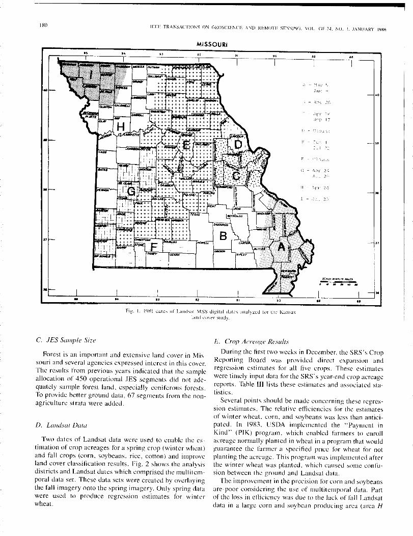
" ~1ay ')
t\uq H
- Apt :20
- !\[Jr
1
• e.- n.JLi I 2~
F -
- i\pl~ 71.fu 1
II - 24•• n_- ell! 1
180
••
IEEE TRANSAC'['[ONS ON GEOSCIENCE AND REMOTF SENSING. VOl.. GE-2.l NO. I. JANUARY 19S6
MISSOURI
••
Fig.!. 1981 dates of Landsat :YISS digital dales analyzed !(lr the Kansasland cover study.
C. JES Sample Size
Forest is an important and extensive land cover in Mis-souri and several agencies expressed interest in this cover.The results from previous years indicated that the sampleallocation of 450 operational JES segments did not ade-quately sample forest land, especially coniferous forests.To provide better ground data, 67 segments from the non-agriculture strata were added.
D. Landsat Data
Two dates of Landsat data were used to enable the es-timation of crop acreages for a spring crop (winter wheat)and fall crops (corn, soybeans, rice, cotton) and improveland cover classification results. Fig. 2 shows the analysisdistricts and Landsat dates which comprised the multitem-poral data set. These data sets were created by overlayingthe fall imagery onto the spring imagery. Only spring datawere used to produce regression estimates for winterwheat.
E. Crop Acreage Results
During the first two weeks in December, the SRS's CropReporting Board was provided direct expansion andregression estimates for all five crops. These estimateswere timely input data for the SRS's year-end crop acreagereports. Table III lists these estimates and associated sta-tistics.
Several points should be made concerning these regres-sion estimates. The relative efficiencies for the estimatesof winter wheat, corn, and soybeans was less than antici-pated. In 1983, USDA implemented the "Payment inKind" (PIK) program, which enabled farmers to enrollacreage normally planted in wheat in a program that wouldguarantee the farmer a specified price for wheat for notplanting the acreage. This program was implemented afterthe winter wheat was planted. which caused some confu-sion between the ground and Landsat data.
The improvement in the precision for corn and soybeansare poor considering the use of multitemporal data. Partof the loss in efficiency was due to the lack of fall Landsatdata in a large corn and soybean producing area (area H
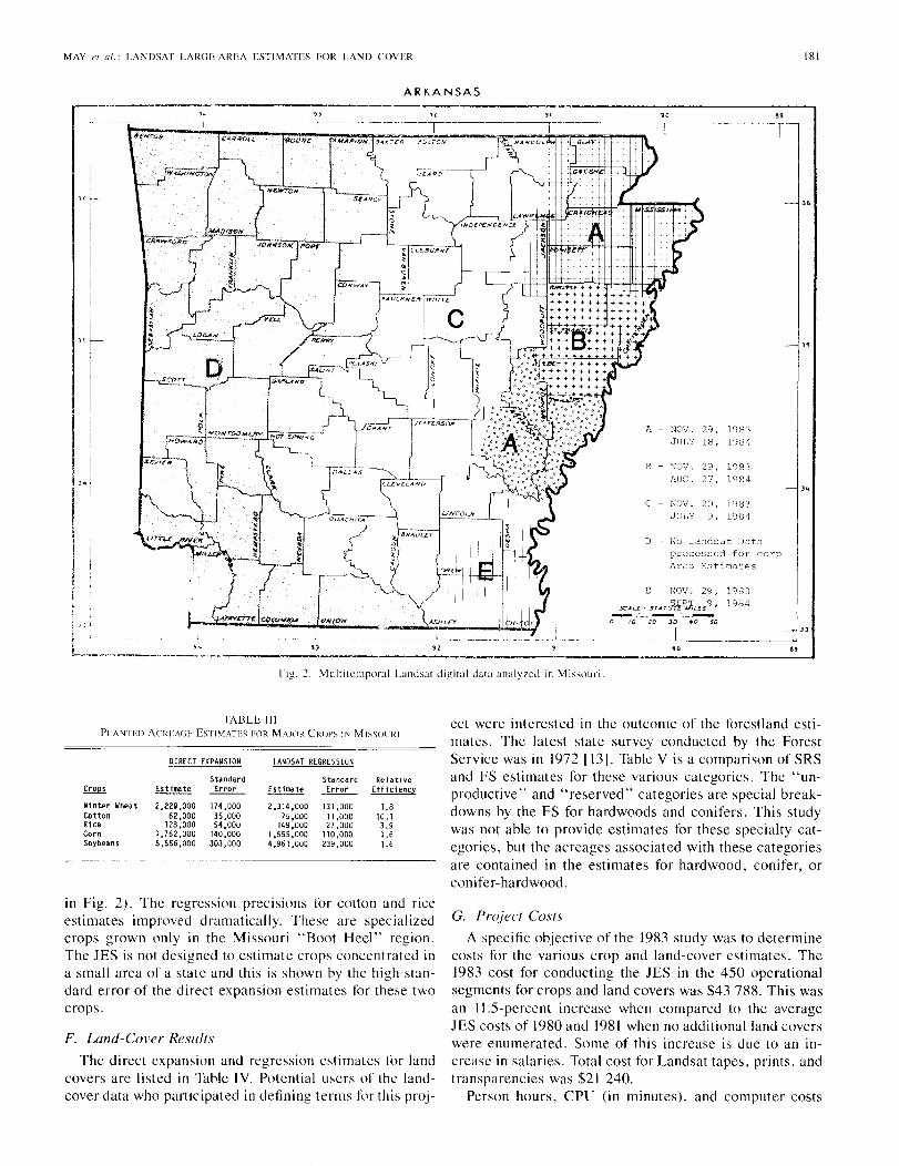
MAY et al.: LANDSAT LARGE-AREA ESTIMATES FOR LAND COVER
ARKANSAS
ISI
A - NOV. 29, 1983JULY 18, 1984
B - ~ov. 29, 1983AUG. 27, J.984
)4
C - NOV. 20, 1983JULY 9, 1984
D - No Lancsat Dataprocessed for corpArea ::::sti'C:1ates
E - r-;ov. 29, 1983SCAt..£ - 5TAn.JSJP •.••~L£S 9 I
1984
"
)5~-
10-
III
,1,,1, _ L_
L.,..-.~,._~ . ":~. " _
"
91
"
1.,
'0
- ---" fO ;0 30 +0 SO
'0
••
••
)6
»
Fig. 2. Multitclllporal Landsat digital data analyzed in Missouri.
TABLE IIIPLA'ITED ACRFNil' ESTIMATES FOR MAJOR CROPS IN MISSOlRI
DlRECT EXPANSION LANDSAT REGRESSION
Standard Standard Rela theCrops Estimate ~ Estimate ~ Efficiency
Winter Wheat 2,229,000 174,000 2,314,000 131,000 1.8COtton 62,000 35,000 75,000 11 ,000 10. ,Rice 128,000 54,000 149,000 27 ,000 3.9Corn 1,762,000 140,000 1,555,000 110,000 1.6Soybeans 5,556,000 303,000 4,961,OOQ 239,000 1.6
in Fig. 2). The regression preCIsions for cotton and riceestimates improved dramatically. These are specializedcrops grown only in the Missouri "Boot Heel" region.The JES is not designed to estimate crops concentrated ina small area of a state and this is shown by the high stan-dard error of the direct expansion estimates for these twocrops.
F. Land-Cover Results
The direct expansion and regression estimates for landcovers are listed in Table IV. Potential users of the land-cover data who participated in defining terms for this proj-
ect were interested in the outcome of the forestland esti-mates. The latest state survey conducted by the ForestService was in 1972 [13]. Table V is a comparison of SRSand FS estimates for these various categories. The "un-productive" and "reserved" categories are special break-downs by the FS for hardwoods and conifers. This studywas not able to provide estimates for these specialty cat-egories, but the acreages associated with these categoriesare contained in the estimates for hardwood, conifer, orconifer-hardwood.
G. PrcJject CostsA specific objective of the 1983 study was to determine
costs for the various crop and land-cover estimates. The1983 cost for conducting the JES in the 450 operationalsegments for crops and land covers was $43 788. This wasan 11.5-percent increase when compared to the averageJES costs of 1980 and 1981 when no additional land coverswere enumerated. Some of this increase is due to an in-crease in salaries. Total cost for Landsat tapes, prints, andtransparencies was $21 240.
Person hours, CPU (in minutes), and computer costs
]82 IEEE TRANSACTJOj\;S ON GEOSCIENCE AND REMOTE SENSING, VOL. GE-24. NO. I. JAj\;UARY 19R6
TABLE IVLAND COVER DIRECT EXPANSION AND RFC;RESSION ESTIMSIES FOR MISSOURI
TABLE VITOTAL RESOURCE RFQUIREME:--iTS EOR DII'I"lRE:--iT LANDSAT" A"'AIYSES USI~(;
A COMMON TEST AREA
TOTAL $106,000
VII. 1984 ARKANSASSTUDY
TABLE VlICOST HlR 1984 ARKANSAS CROP A:--iD LAND COVER PROJECT
B. Project CostsThe additional costs over normal JES costs for con-
ducting this project are given in Table VII. These costswere evenly divided between the three agencies.
ComputerCost
T"T,RT12,634
20,481
CPU(min. )/T'J"
1,294
2,380
Person-hours237467
707
~~~~~~~ra 1 Wi nter Wheat"uHitempora 1 SlIlI1Ier Cropsl1ul t1 tempora 1 Summer Crops and Land
Coyers
A. Objectives
Land-cover results obtained from the Kansas and Mis-souri studies generated interest within the Soil Conser-vation Service and Forest Service. These two agenciesalong with the SRS jointly defined and funded a crop andland-cover study in Arkansas. The overall objectives ofthis study were to I) utilize SRS's ground data collectionand Landsat analysis techniques to produce a crop andland-cover classification for the entire state and 2) providethis classification on tapes so that each agency could in-dependently utilize the land-cover data in their respectiveprograms.
The SRS used the classified data to obtain 1984 plantedacreage estimates for cotton, rice, soybeans, and sor-ghum. SCS will use the classified data in their next na-tional resources inventory and FS will utilize the data Intheir forest land inventory.
tape and the utility of the classified data are being assessedby potential users of the land-cover data, Increasing thesample allocation of the regular JES provided improvedestimates of forest categories due to more samples in theforest strata. Cost figures were kept for all analysis stepsand the additional cost of doing land cover was deter-mined. The increase in precision of crop and land-coverestimates, when using multitemporal Landsat data, wasnot as high as originally anticipated. Research is neededto determine if the addition of land covers had an adverseaffect on the classification results of summer crops.
MATUlIALSLandsat Data - ~17 ,000 (~730x20 scenes + B/W Prints)Blank Tapes - ~ 2,000 ('25 x 80l
DATA PROCESSINGHartjn Marietta - $2,000 (ground data)ARPANET - ~4,OOO (Electronic data transmissions)IBM 33-30 - $2.000 (tape reformat & data editing)OEC-I0 - ~36,OOO (muHitemporal overlay, di9itlzing, registra-
tion. signature development)CRAY-IS - $8,000 (full scene classification)
PERSONNEL--oat. Analyst - ~25,OOO 0/2 HYE at GS13)Support Staff - $10,000
Ca t,,~ SRS FSHar<'l<ood 11,139,532 11 ,619 ,900
Confer 187,650 204,300
Con"er-Hardwood 1,148,447 540,500
(Unwoductive) (included above) 298,300
(Resl!rved) (included above) 256,100
TOTAL 12,475,629 12,919,100
Grazed Forest 2,705,512 2,803,100
DIRECT EXPANSION REGRESSION
Standard Standard Relat1ve
Cover Estimate Error Estimate ~ Efficiency
Hardwood 10,499,754 529,061 11,139,532 443,461 1.4Coni fer 181,568 43,325 187,650 21,782 4.0
Con 1fer-
Ha rowood 1,149,738 247,934 1,148,447 245,461 1.0
Grazed Forest 2,884,732 297,743 2,705,512 299,958 1.0
Brushland 1,286,435 143,382 1,318,875 138,723 1.1
Row Crops 8,539,851 361,734 7,742,383 24~ ,344 2.2
Sown Crops 2,391,119 175,337 2,547,815 127,349 1.9
Idle/cropland 2,100,277 163,574 2,015,582 139,389 1.4Hay 3,110,286 197,393 2,980,606 171,303 1.3
Cropland/
Pas ture 1,434,850 234,325 1,245,797 149,895 2,4
Other Pasture 7,698,684 423,699 7,624,049 380,381 1.2
Idle Grassland 1,403,300 140,411 1,331,205 133,127 1.1
Farmsteads 385,091 23,474 387,434 23,515 1.0
Residentia 1 962,910 105,045 823,018 95,629 1.2
Corrmerc 1a 1 328,253 81,590 305,556 41,463 3.9
Other Urban 140,229 39,114 122,873 30,365 1.7
Transportation 296,577 53,422 288,724 53,398 1.0
lakes 307,755 118,936 265,246 108,556 1.2Ponds 84,270 17,563 84,438 13,130 1.8
Rivers 129,922 43,887 103,729 23,368 3.5
Disturbed land 44,223 17,741 42,455 16,020 1.2
Transitional 183,379 137,668
",etlands 106,830 87,386
'Fields that are double crOpped are included in the estimates for each crop.
TABLE VCOMPAIHSO:--i OF 1983 FORESTLAND ESTIMATES FROM SRS LANDSAT STUDY
WITH ]972 FOREST SERVICE ESTIMATES
were recorded for various steps required to process theLandsat data and to generate regression estimates. Thesesteps and associated costs were tracked separately forwinter wheat, summer crops, and land covers.
In this study, winter wheat was analyzed using unitem-poral spring Landsat data. A second analysis using mul-titemporal spring and fall data was done for summer cropsand land covers. Table VI presents the total resource re-quirements for Landsat analysis. Analyzing and estimat-ing the 23 land covers with summer crops required 51 per-cent more person hours and a 62-percent increase incomputer cost. A majority of these costs were incurredduring the acreage estimation processes. Since this studythese estimation programs have been rewritten whichshould reduce future costs of producing land-cover esti-mates.
In summary, 23 land covers and five major crops wereclassified and estimated. The classifications were saved on

MAY el al.: LANDSAT LARGE-AREA ESTIMATES FOR LAND COVER
KANSAS
183
N
. RA
NY
A - June 17
B - April 25
C - August 11
D - May 14E - May 24
F - April 27
G - August 31
H - July 9
I ~ June 21
Fig. 3.
J ~ July 10
TABLE VIIIDIRECT EXPANSION AND REGRESSION ESTIMATES FOR MAJOR CROPS IN
ARKANSAS
DIRECT EXPANSION LANDSAT REGRESSIONStandard Standard Relative
~ Estimate ~ ~ ~ Efficiency
Cotton 442,000 94,000 458,000 61,000 2.4Rice 1,161,000 118,000 1. 133.000 69,000 2.9Soybeans 4,124,000 204,000 3,989,000 136,000 2.3Sor9hum 671,000 85,000 559,000 60,000 2.0
C. Land Cover DefinitionsRepresentatives from the three agencies met and estab-
lished the terms and definitions for the survey. A listingof the land cover classification categories are shown be-low:
date of the multitemporal data set. The second date ofLandsat data were obtained from summer and fall 1984.Most of the crop land is located in the eastern half of Ar-kansas. To meet the SRS due dates for crop estimates,eastern Arkansas was analyzed first. Fig. 3 delineates theanalysis districts and Landsat dates.
E. Results
The direct expansion and regression estimates for thecrops generated for the SRS are given in Table VIII. Theseestimates were produced and delivered on December 1 intime for the year-end crop acreage report. The land-coverestimates and classified tapes for the SCS and FS will begenerated during the first quarter of 1985. Therefore, theseresults were not available for inclusion in this paper.
D. Landsat DataMultitemporal Landsat data were obtained for most of
the state. Conifers are an important land cover; therefore,late fall 1983 and winter 1984 were obtained for the first
Hardwood ForestMixed ForestConifer ForestClearcut ForestBarren LandUrbanWater
Native PastureImproved PastureRow CropsSown CropsHayOther Land Use
VIII. CONCLUSIONSFive years of research were conducted in developing and
evaluating techniques for obtaining large-area land-coverclassifications and area estimates. The remote-sensingtechniques developed by the USDA's SRS for improvingcrop area estimates formed the basis forthis research. Theoverall objective of applying this technology for the pur-pose of obtaining land-cover information was met. Thefollowing are specific conclusions from the land-cover re-search.
1) SRS's JES provides a vehicle, on an annual basis. for
184 IEEE TRANSACTIONS ON GEOSCIENCE AND REMOTE SENSING. VOL. GE-24. NO. I. JANUARY 1986
obtaining ground truth data for land cover surveys thatutilize Landsat data.
2) For classification and estimation purposes the oper-ational JES segment allocation does not adequately samplemany noncrop cover types. This can be corrected by in-creasing the sample size in strata for which the landcover(s) are located.
3) The SRS's deadline for timely crop area estimatescan still be met when noncrop covers are included in thesurvey and Landsat analyses.
4) Two products can be obtained from the techniquesdiscussed in this report: a) acreage estimates with mea-sures of precision and b) classified Landsat data containedon tapes.
5) The utility of classified Landsat data for land-coverstudies by other federal and state agencies is still beingassessed.
6) Large increases in computer time and person hourswere incurred when analyzing noncrop covers with crops.This can be offset by multiple agencies sharing the cost ofa crop and land-cover survey.
REFERENCES
III J. R. Anderson, E. E. Hardy, J. T. Roach, and R. E. Witmer, "A landuse and land cover classification system fi)f use with remote sensordata," Geological Survey Professional Paper 964, U.S. Dep\. of In-terior, 1976.
12] G. H. Ball and D. J. Hall, "A e1ustering technique for summarizingmultivariate data," Behavioral Sci., vol. 12, pp. 153-155, 1967.
131 c. E. Caudill, "Current methods and policies of the statistical re-porting service," in Proc. Symp. Machine ProcessinR of RemotelySensed Data (West Lafayette, IN), pp. 1-5. 1976.
141 P. w. Cook, "Landsat registration methodology used by U.S. De-partment of Agriculture's Statistical Rep()f1ing Service 1972-1982."U.S. Depm1ment of Agriculture, Statistical Rcporting Service Tech.Rep., presented at the American Statistical Association Meetings,Cincinnati, OH, 1982.
15J M. L. Holko, "1982 results tiJr the Calililrnia cooperative remotesensing project," Statistical Reporting Service. U.S. Dep. of Agri-culture. Washington, DC, 1984.
(6] E. E. Houseman. "Area sampling in agriculture," U.S. Dep. of Ag-riculture, Statistical Reporting Service, SRS-20, 1975.
17] D. D. Klcwcno and C. E. Millcr, "1980 AgRISTARS DC/LC ProjcctSummary: Crop area cstimates lilr Kansas and Iowa," U.S. Dep. ofAgriculture, Statistical Reporting Service, AGESS-810414, 1981.
18] R. K. Lennington and M. E. Rassback, "Classy~An adaptive maxi-mum likelihood clustering algorithm," in Proc. LACIE Svmp. (Hous-ton, TX), pp. 671-690,1978.
19] J. Mergerson, C. Miller, M. Ozga, M. Holko, S. Winings, P. Cook,and G. Hanuschak, "1981 AgRISTARS DCLC four statc projcct." inProc. Svmp. Machine ProcessinR of Remolely Sensed Data (West La-fayette, IN), pp. 34-44. 1982.
110] NASA, "Earth rcsourccs laboratory applications software," Earth Rc-sourccs Lab. Rep. 183, National Space Tcchnology Lab., MS, 1980.
[II] M. Ozga and W. E. Donovan, "An intcractivc systcm for agriculturalacreagc estimates using Landsat data," in Proc. Svmp. Machine Pro-cessing of Remolely Sensed Data (West Lafayettc, IN), pp. 113--123,1977.
112] R. S. Sigman, G. A. Hanuschak, M. E. Graig, P. W. Cook, and M,Cardenas, "The use of regression estimation with Landsat and prob-ability ground sample data," U.S. Dep. of Agriculture, Statistical Re-porting Service Tech. Rep., presented at the Amcr. Statistical Asso.Mectings, San Diego, CA, 1978.
113] J. S. Spencer and B. L. Esscx, "Timber in Missouri," USDA ForcstService Rcs. Bull. NC-20, North Central Forest Experiment Station,S\. Paul, MN, 1976.
(14] S. B. Winings. P. W. Cook, and G. A. Hanuschak, "1982 corn andsoybean area estimates j(,r Iowa and Illinois," U.S. Dep. of Agricul-ture, Statistical Rcporting Scrvice Tceh. Rep., prcscntcd at thc 17thInl. Symp. on Remote Sensing of Environment, Ann Arbor, MI. 1983.
*
George A. May received the B.S., M.S., andPhD. degrees in agronomy from The PennsylvaniaState University, University Park, PA, in 1971,1973, and 1976, respectively.
From 1976 to 1980, he was a remote sensi ngspecialist assigned to the Large Area Crop Inven-tory Experiment (LACIE), in Houston, TX, andwas involved in AgRISTARS from 1981 to 1984.Currently, he is an Agricultural Statistician withthe U.S. Department of Agriculture involved in re-mote-sensing-data application in Calili)rnia.
*
Martin L. Holko received the B.S. degree in for-est science from The Pennsylvania State Univer-sity, University Park, in 1973, and the M.S. de-gree in mathematical statistics from MichiganState University, East Lansing, in 1980.
He was an Agricultural Statistician with thcU.S. Depm1mcnt of Agriculture, Statistical Rc-porting Service, assigned to the New York StateStatistical Of lice (SSO) from 1973 to 1976, theNew England SSO from 1976 to 1978, and theMichigan SSO from 1978 to 1980. He has been a
Mathematical Statistician with the U.S. Department of Agriculture:SRS:SRD:RSB since 1980. He is currently involved in the application ofremotely sensed data and microprocessor technology to area frame devel-opment.
*
Ned Jones, Jr., received the B.S. and M.S. de-grees from the Virginia Polytechnic Institute andState University, Blacksburg, in 1971 and 1977,respectively. From 1982 to 1983 he did graduatework in statistics at North Carolina Stale Univer-sity, Raleigh.
He was a Commodity Stalistician with the U.S.Department of Agriculture, Statistical ReportingService, assigned to the Kentucky State StatisticalOftice (SSO) from 1977 to 1981. and Ihe NorthCarolina SSO from 1981 to 1983. Since 1983, he
has been a Mathematical Statistician with the USDA:SRS:SRD:RSB.

Authors must enclose a signed copy of this form whensubmitting manuscripts to the Editor of this journal.
IEEE COPYRIGHT FORM
Signed form, appropriately completed, MUST ACCOMPANY any paper to be published by IEEE.PLEASE READ REVERSE OF THIS FORM FOR FURTHER DETAILS.
TITLE OF PAPER:
AUTHOR(S):
PUBLICATION TITLE: IEEE Transactions on Geoscience and Remote SensingMONTH AN D YEAR:
RETURN FORM TO:
PART A - COPYRIGHT TRANSFER FORM(NOTE: Company or other forms may not be substituted for this form. U.S. Government employees whose work is not subject to copyrightmay so certify by signing Part B below.)
The undersigned, desiring to publish the above paper in a publication of the IEEE or cosponsored by the IEEE,hereby transfer their copyrights in the above paper to The Institute of Electrical and Electronics Engineers, Inc.,known as the IEEE.
Returned Riahts: In return for these rights, the IEEE hereby grants to the above authors, and the employers forwhom the work was performed, royalty-free permission to:
1. Retain all proprietary rights other than copyright, such as patent rights.2. Reuse all or portions of the above paper in other works.3. Reproduce, or have reproduced, the above paper for the author's personal use or for company use provided
that (a) the source and IEEE copyright are indicated, (b) the copies are not used in a way that implies IEEE en-dorsement of a product or service of an employer, and (c) the copies per se are not offered for sale.
4. Make limited distribution of all or portions of the above paper prior to publication.5. In the case of work performed under U.S. Government contract, the IEEE grants the U.S. Government royalty-
free permission to reproduce all or portions of the above paper, and to authorize others to do so, for U.S. Govern-ment purposes.IEEE Obliaations: In exercising its rights under copyright, the IEEE will make all reasonable efforts to act in theinterests of the authors and employers as well as in its own interest. In particular, the IEEE requires that:
1. The consent of the first-named author be sought as a condition in granting republication permission toothers.
2. The consent of the undersigned employer be obtained as a condition in granting permission to others to re-use all or portions of the paper for promotion or marketing purposes.
In the event the above paper is not accepted and published by the IEEE or is withdrawn by the author(s) before ac-ceptance by the IEEE, this agreement becomes null and void.
AUTHORIZED SIGNATURE
EMPLOYER FOR WHOM WORK WAS PERFORMED
TITLE IF NOT AUTHOR
DATE FORM SIGNED
PART B - U.S. GOVERNMENT EMPLOYEE CERTIFICATION(NOTE: If your work was performed under Government contract but you are not a Government employee, sign transfer form above and seeitem 5 under Returned Rights.)
This will certify that all authors of the above paper are employees of the U.S. Government and performed thiswork as part of their employment and that the paper is therefore not subject to U.S. copyright protection.
AUTHORIZED SIGNATURE
NAME OF GOVERNMENT ORGANIZATION
TITLE IF NOT AUTHOR
DATE FORM SIGNEDU-102

IEEE COPYRIGHT FORM(continued)
Information to Authors
IEEE POLICY
Thank you for your interest in the IEEE. As you know, the IEEE distributes its technical publications throughoutthe world, and it is necessary to translate and abstract its publications, and articles contained therein, for inclu-sion in various compendiums and similar publications, etc. When an article is submitted for publication by theIEEE, the IEEE understands that its acceptance of the article implies that the IEEE has the rights to do all of thethings it normally does with such an article.
In connection with its publishing activities, it is the policy of the IEEE to own the copyrights in its technicalpublications, and to the contributions contained therein, in order to protect the interests of the IEEE, its authorsand their employers, and at the same time to facilitate the appropriate re-use of this material by others.
The new United States copyright law requires that the transfer of copyrights in each contribution from the authorto the IEEE be confirmed in writing. It is therefore necessary that you execute either Part A-Copyright TransferForm or Part B-U.S. Government Employee Certification on the reverse side of this sheet and return it to theEditor (or person who supplied this sheet) as promptly as possible.
AUTHOR/COMPANY RIGHTS
If you are employed and you prepared your paper as a part of your job, the rights to your paper initially rest withyour employer. In that case, when you sign the copyright transfer form, we assume you are authorized to do so byyour employer and that your employer has consented to all of the terms and conditions of this form. If not, itshould be signed by someone so authorized.
NOTE RE RETURNED RIGHTS: Just as the IEEE now requires a signed copyright transfer form in orderto do "business as usual," it is the intent of this form to return rights to the author and employer so thatthey, too, may do "business as usual." If further clarification is required, please contact: Ms. PatriciaPenick, Manager, Publication Administrative Services, IEEE, 345 E. 47th St., New York, NY 10017 (212)705-7550.
JOINT AUTHORSHIP
For jointly authored papers, only one signature is required, but we assume all authors have been advised andhave consented to the terms of this form.
U.S. GOVERNMENT EMPLOYEES
Authors who are U.S. Government employees are not required to sign the Copyright Transfer form (Part A), butany co-authors outside the Government are.
Part B of the form is to be used instead of Part A only if all authors are U.S. Government employees and preparedthe paper as part of their job.
NOTE RE GOVERNMENT CONTRACT WORK: Authors whose work was performed under a U.S.Government contract but who are not Government employees are required to sign Part A-CopyrightTransfer Form. However, item 5 of the form returns reproduction rights to the U.S. Government when re-quired Aven though the IEEE copyright policy is in effect with respect to the reuse of material by thegeneral public.
Thank you for your prompt cooperation.
OCTOBER 1978

Now is thebest timeto join oursociety.
It's always time to upgrade yourcareer. Membership gives youready access to state-of-the-artmeetings and conferences in yourareas of interest, and to their pub-lished proceedings. You get tomeet experts from other organiza-tions and to participate in technicalactivities with the prime movers inengineering, science and business.Our membership is worldwide.
At least one periodical is included
............... - .. - -, ....... '"' , .
in your Society fee, keeping youabreast of the latest developmentsin your field. And, as an IEEEmember, you may choose from awide range of books, Standards,conference records, employmentsurveys, short courses and othercareer-building aids-all at dis-counted member prices.
MEMBERSHIP APPLICATION
Please take this opportunity, now,to broaden your outlook, open yourmind to new concepts, new tech-niques, new fields of interest. Therewill be no better time. Return theMembership Application formbelow. (Students should contacttheir IEEE counselor or write for aStudent Membership brochure.)
.............. , .............................................., , .
I am applying for the following as indicated:o I am an IEEE member. Please enroll me in the above Society.
IEEE member No.D=rIILDo IEEE membership plus Society membership.o IEEE membership only.
+IEEEGEOSCIENCE ANDREMOTE SENSINGSOCIETY
Please check appropriate box(es) below:
All dues and fees below (except for theIEEE entrance fee) are annual rates. Indi-cate here whether you are remitting ei-ther 100% or 50% of these rates. (Seechart above.)
0100% 050%
Society fee: $7.00 0 $ _(Includes Transactions onGeoscience and RemoteSensing)
IEEE entrance fee (for non-IEEE members only): Remit$15.00 regardless of monthof application. 0 $ _
IEEE membership annualdues and (if applicable)Regional assessmentpayments
Full signature
First name (print) Middle initial(s)
Date
Last name
U.S. (Region 1-6) $67.00 0 $ _
Canada (Region 7) $62.00 0 $ _
Europe, Africa & Mid. East(Region 8) $59.00
APPLICANTS FOR IEEE MEMBERSHIPPLEASE COMPLETE THE FOLLOWING INFORMATION:Date of birth _
Month Day Year 0 Male 0 FemaleWere you ever a member of IEEE? 0 Yes If Yes, please furnish (if known):
ONo
EDUCATION (Highest level completed):
Latin America(Region 9) $52.00
Asia & Pacific(Region 10)$53.00
PAYMENT ENCLOSED
O$~~
O$~~
O$~~
O$~~
Street address
Name of educational Institution
State/Country
Grade
Postal Code
Membership No.
Remit in U.S. dollars drawn on a U.S. bank.Make check payable to IEEE. Course Degree received Date
Please mail to:IEEE Service Center445 Hoes LanePiscataway, NJ 08854-4150 U.S.A.(201) 981-1393
ENDORSEMENT (Signature of one IEEE member. who knows you professionally.)TRACKING CODE
56575859W61~63~65W~ 6869ro71nnu~M77n
..... - ... .. .

Presentingthe first title in the new
NEXT-GENERATIONCOMPUTERS
It's possibly the most important book you could own.
A concise and comprehensive examinationof next-generation computer technologies,the worldwide effort to advance them, thelikely technical and sociotechnical fallout.
The technology is not yet in place forthe 50-called "fifth" generation of user-friendly, superfast and supersmart com-puters. But it will soon come to pass.
Multiprocessors artificial intelli-gence ... networking--fundamental break-throughs in every sector of computerscience will be needed to achieve this newclass of computers capable of processing
AT&T Technologies,Ine. manufacturesa memory chipthat can store aquarter of a mil-lion bits ofinformation.
Are you-is your company-prepared to compete in theupcoming technological revolution?
NEXT-GENERATION COMPUTERS revealshow the new computer capabilities arelikely to change the way you perform yourjob, the new products you are likely to takepart in designing, the various ways your joblife could be affected.
The impending revolution has a greaterpotential to alter your career path, to repo-sition your company in the marketplace,than any technological advance in ourlifetime.
This book will increase your awarenessof the opportunities and pitfalls that couldlie ahead, will help you and your company'smanagement to make informed, intelligentdecisions about the parts you will be play-ing in the scenario of things to come.
Don't pass up this opportunity. Send foryour copy today.
'iA choice to delayor not to adopt
~ these technologies" • is equivalent to
'" , 0 accepting a signifi-
~
canlly lower stand-• \ ard of living.
M. Granger Morgan,- ' 'Carnegie-Mellon U.
ligence. computer vision. expert systems,and many more.• A speCial tutorial review section thatprovides a solid foundation In each of themajor technologies.• A look at the competing teams andplayers worldwide who are intent on beingfirst with tomorrow's machines, includingtime-lines showing the probable develop-ment of constituent tpchnologips.• An in-clPpth analYSIS by Ipadingenginpers. scipntists dnd technology-watchers on what the future is likely to hold
symbolic information a thousand timesfaster than anything we have today.
In the U.S., in Europe and Japan.governments and R & D centers have budg-eted billions in a determined effort todominate the impending informationrevolution.
At stake: World supremacy of theadvanced-computer and high-technologymarkets of the 1990s and beyond.
About this bookBased in part on articles in the Spec trumspecial issue "Tomorrow's Computers,"NEXT-GENERi\TION COMPUTERS includescontributions by 40 recognized leaders inartificial intelligence, hardware and soft-ware, architecture, and technology assess-ment. Major features include.• A review of current developments in thekey, emerging technologies of artificial intel-
Spectrum SeriesThis is the first title in the new SpectrumSeries of books to be published by the IEEEPRESS. Upcoming volumes will be single-topic books dpvoted to such ,Heas as designcasp histories. innovation, engineeringmanagenlPnt and rptrosppctlve themes.Each volume will be prodlJ( eel by the expt'rteditors who have earn"d for Spec trum twoNational Magazirw Awards for "xcellence.
-------------------------
Meet the Next Generation NOW. Use this coupon.
NEXT-GENERATION COMPUTERSAn IEEEPRESSSpectrum Sl'ril's Book. 1985.360 Pl'. 12') i1lu,trat;ons. ISBl"mIUl7<J42-1<)4-()List: 539.95; IEEEMernhpr: $35.(L=),First COpy' only ror pe{'\of1,Ji USf'.. '\cJdiliunai ((J{lIP,> at /i'>t
Postal COdl'
MelillO
IEEE S£'rvin' CentN44') Ho('., LdlW
PI"C,ll.lW,lY, NJ OHHS441')() l;.S.A.
IEEE No.
City
Addres{,
Name (print)
State/Country
Bill me. (A $2.00 billing dldrgc is addpd toall non-Lclsh dnd nO[l-nl'dit (drd orders undt'rSl()()()())
•IEEESignature
Exp. Date
Card No.
Yes, plf'ase send me copy (ips) ofNEXT-GENERATIOI" COMPUTERS(PC018831 right away. List: 539.9'): la~1\1cmher $35.95 (Ursl COP}' only'.;
Purchase amounL $ .}\i'e~'v jerspy' residents add sd/ps tax
[J Payment enclosed. ('--lake check payableto IEEEIII US dollars drawn on a US bankl
Charge thl' credit card Indicated'n MasterCard/Eurocard 1.1 V,sa[] American Express

INFORMATION FOR AUTHORS
Subject Matter: The IEEE TRANSACTIONS ON GEOSCIENCE AND REMOTE SENSING is concerned with the publication of both theoreti-cal and applied papers on geoscience and remote sensing. Papers should relate to the field of interest of the IEEE Geoscience and RemoteSensing Society, which is "the theory, concepts, and techniques of science and engineering as applied to sensing the earth, oceans, atmosphere,and space, and the processing, interpretation, and dissemination of this information."
Membership in IEEE or associated technical organizations is not required of authors.
Papers: Except in the case of review or tutorial papers, the technical content of papers should be both new and significant. Experimentaldata should be complete and should include sufficient description of experimental apparatus, methods, and relevant experimental condi-tions.
Process for Submitting Papers: Five copies (original plus four copies) of the manuscript should be submitted to the appropriate ExecutiveEditor or Associate Executive Editor. In addition, five copies of the illustrations should be provided and an abstract of not more than 200words.
Style for Manuscript: This TRANSACTIONS is addressed to readers with a wide variety of interests. Few will be expert in the author's field.Consequently, authors should refrain from using or should take care to explain any terminology which may not be familiar to such readersand should provide brief introductory remarks and references which will permit the reader to relate the paper to other work in the author'sfield of specialty. Clarity of both writing and illustrations is required of all authors.
Manuscripts should be limited to twenty-five double-spaced typewritten pages, on one side of the sheet only, with a maximum of fifteenfigures. Specific references should be numbered footnotes, appearing on the page where cited; general references should be numbered andshould appear in order of reference at the end of the paper. A separate bibliography, listed alphabetically, may be added. References shouldbe complete and in the IEEE style. (See "Information for IEEE Authors," available from the IEEE Publications Department, 345 East47th Street, New York, NY 10017.)
Illustrations should be provided in quintuplicate with titles and numbers typed on a separate sheet. If the paper is accepted, originalillustrations will be required. (See Rel'iew Process, below.)
Review Process: Papers are reviewed by qualified referees. Decisions on disposition of the manuscript are made in six weeks. The author isthen notified of the decision. If the paper has been accepted, originals of the illustrations, a photograph of the author, and a short biographyof the author are requested at this time.
Voluntary Page Charges: After a paper has been accepted, the author's organization will be requested to pay a voluntary charge of $11 0 perprinted page to cover part of the cost of the publication. The author will receive 100 reprints of his paper or communication if the pagecharge is honored.
Excessive Paper Length Charges: A mandatory Excessive Paper Length charge of $125.00 per page is required for papers longer than six(6) printed pages. The author will be notified of the estimated paper length upon Receipt of the original manuscript. The author will berequested, conditional upon favorable technical review, to pay Voluntary Page Charges for all pages and Mandatory Excessive PaperLength Charges. If the author will not agree to pay mandatory charges, the author will be required to reduce the manuscript to six printedpages or less prior to final acceptance and scheduling for publication. This reduction will occur after technical review of the manuscript. Theabove policy has no relationship to requests by the Editor to reduce very long manuscripts prior to technical review.
Brief Papers and Letters Tothe Editor: These items should be prepared and submitted according to the instructions given above for regularpapers, but for these changes: they should not exceed five pages; they should not contain more than three illustrations; abstracts should belimited to 50 words.
Copyright: It is the policy of the IEEE to own the copyright to the technical contributions it publishes on behalf of the interests of the IEEE,its authors, and their employers, and to facilitate the appropriate reuse of this material by others. To comply with the U.S. Copyright Law,authors are required to sign an IEEE copyright transfer form before publication. This form, a copy of which appears in the January 1985issue of this Transactions, returns to authors and their employers full rights to reuse their material for their own purposes. Authors mustsubmit a signed copy of this form with their manuscripts.
Submit Correspondence for Manuscripts.Brief Papers. Letters to the Editor to:
Prof. Fawwaz T. UlabyEditorThe University of Michigan Radiation LaboratoryDepartment of Electrical and Computer Engineering4072 East Engineering BuildingAnn Arbor, MI 48109
INSTITUTIONAL LISTINGSThe IEEE Geoscience and Remote Sensing Society invites application for Institutional Listingsfrom firms interested in geoscience and remote sensing.
An Institutiooal Listing recognizes contributions to support the publication of tbe IEEETRANSACTIONS ON GEOSCIENCE AND REMOTE SENSING. Minimum.rates are $50.00 forlisting in one issue; $200.00 for six consecutive issues. Larger contributions will be most welcome.No agency fee is granted for soliciting such contributions. Inquiries, or contributions madepayable to the IEEE, plus instructions on bow you wish your latitutional Listing to appear,should be sent to TAD Finance Office, The Institute of Electrical and Electronics Engineers,345 East 47 Street, New York, NY 10017.