ieee transactions on computers, vol. 54, no. 7, july...

An On-Chip IP Address Lookup AlgorithmXuehong Sun and Yiqiang Q. Zhao, Member, IEEE

Abstract—This paper proposes a new data compression algorithm to store the routing table in a tree structure using very little

memory. This data structure is tailored to a hardware design reference model presented in this paper. By exploiting the low memory

access latency and high bandwidth of on-chip memory, high-speed packet forwarding can be achieved using this data structure. With

the addition of pipeline in the hardware, IP address lookup can only be limited by the memory access speed. The algorithm is also

flexible for different implementation. Experimental analysis shows that, given the memory width of 144 bits, our algorithm needs only

400kb memory for storing a 20k entries IPv4 routing table and five memory accesses for a search. For a 1M entries IPv4 routing table,

9Mb memory and seven memory accesses are needed. With memory width of 1,068 bits, we estimate that we need 100Mb memory

and six memory accesses for a routing table with 1M IPv6 prefixes.

Index Terms—Algorithms, hardware, tree data structures, range search, IP address lookup, on-chip memory.

�

1 INTRODUCTION

THE Internet system consists of Internet nodes andtransmission media which connect Internet nodes to

form networks. Transmission media are responsible fortransferring data and Internet nodes are responsible forprocessing data. In today’s networks, optical fibers are usedas transmission media. Optical transmission systemsprovide high bandwidth. It can transmit data in severalgigabits (OC48=2.4Gb/s and OC192=10Gb/s are commonand OC768c=40Gb/s is the goal of the near future) persecond per fiber channel. Dense Wavelength DivisionMultiplexing (DWDM) [11] technology can accommodateabout 100 channels (2004) and possibly more in the future inone strand of fiber. This amounts to terabits per secondtransmission speed on optical fiber. In order to keep pacewith this speed, the Internet nodes need to achieve the samespeed of processing packets. The Internet nodes implementthe functions incurred by the Internet system. The fourmain tasks of the Internet nodes are IP address lookup(and/or packet classification), packet modification, queue/policy management, and packet switching.

Given the smallest packet size of 40 bytes (worst case), inorder to achieve 40 Gigabits per second (OC768) wire speed,the router needs to lookup packets at a speed of 125 millionpackets per second. This, together with other needs inprocessing, amounts to less than 8ns per packet lookup.Nowadays, one access to on-chip memory takes 1-5ns forSRAM and about 10ns for DRAM. One access to off-chipmemory takes 10-20ns for SRAM and 60-100ns for DRAM.This figure shows that the development of high-speed IPlookup algorithms which can be implemented on chip is ingreat demand. It also shows that it is very difficult for serial

algorithms to achieve the ideal wire speed. Developingalgorithms that integrate parallel or pipeline mechanismsinto hardware seems a must for future Internet Protocol (IP)address lookup.

Industry responded to the aforementioned demand byoffloading the processing tasks to coprocessors [20]. Acoprocessor is a system on a single chip to perform a singletask. Previously, the general purpose processor was used inthe Internet nodes. Recently, Network Processors [23] aregaining popularity in processing Internet data. The trend isto use a chip to exclusively perform the IP lookup task. Asmentioned above, one of the advantages of an on-chipsystem is that the on-chip memory access latency is verylow. Another advantages of on-chip systems is larger buswidth to on-chip memory than that to off-chip memory. Thenumber of pins of the chip is smaller if the memory goes onchip rather than off chip. The memos width to on-DRAMcan be more than 1,000. The number of pins for off-chipmemory would increase a lot with the same memory width.

The restriction of an on-chip system is that the memorycannot be large. Reference [19] shows that, for theembedded DRAM, the maximum macro capacity/size is72.95 Mb/31.80mm2 with random access time of 9.0ns usingthe Cu-08 process; for the embedded SRAM, the maximummacro capacity is 1 Mb with random access time of 1.25nsusing the Cu-11 process.

We develop an IP address lookup algorithm which usesa small amount of memory. With this merit, the algorithmcan be implemented in one single chip. Our approach is toconvert the longest prefix match problem into a rangesearch problem [9], [16], [10] and use a tree structure to dothe search. Our main contribution is the development of anovel prefix compression algorithm for compactly storingIP address lookup table. The following techniques are usedin the compression algorithm: 1) We compress the keys in atree node, 2) we use a shared pointer in a tree node, and3) we use a bottom-up process from the leaf to the rootscheme to build the tree.

The rest of the paper is organized as follows: In Section 2,IPv4 and IPv6 address architectures are introduced.Section 3 gives a hardware design reference model for ouranalysis. In Section 4, we give the concepts and definitions

IEEE TRANSACTIONS ON COMPUTERS, VOL. 54, NO. 7, JULY 2005 873

. X. Sun is with the Canadian Space Agency and can be reached at 311 200De Gaspe, Verdun, Quebec Canada H3E 1E6.E-mail: [email protected].

. Y.Q. Zhao is with the School of Mathematics and Statistics, CarletonUniversity, 1125 Colonel By Drive, Ottawa, Ontario Canada K1S 5B6.E-mail: [email protected].

Manuscript received 5 Mar. 2004; revised 3 Dec. 2004; accepted 26 Jan. 2005;published online 16 May 2005.For information on obtaining reprints of this article, please send e-mail to:[email protected], and reference IEEECS Log Number TC-0075-0304.

0018-9340/05/$20.00 � 2005 IEEE Published by the IEEE Computer Society

related to the range search problem. Details of our newalgorithm are presented in Section 5. Results from anexperimental study are presented in Section 6. In Section 7,we highlight comparison results with some existing algo-rithms. Concluding remarks are made in Section 8.

2 IP ADDRESS LOOKUP PROBLEM

Internet Protocol (IP) defines a mechanism to forwardInternet packets. Each packet has an IP destination address.In an Internet node (Internet router), there is an IP addresslookup table (forwarding table) which associates anyIP destination address with an output port number (or next-hop address).When a packet comes in, the router extracts theIPdestination field anduses the IPdestinationaddress to lookup the table to get the output port number for this packet. TheIP address lookupproblem is to studyhow to construct adatastructure to accommodate the routing table so that we canfind the output port number quickly.

Since the IP addresses in a lookup table have specialstructures, the IP address lookup problem can usetechniques that are different from that used to solve generaltable lookup problems by exploiting the special structuresof the IP addresses. Nowadays, IPv4 address is used. IPv6address could be adopted in the future. We next introducethese two address architectures.

2.1 IPv4 Address

An IPv4 address is 32 bits long. It can be represented indotted-decimal notation: 32 bits are divided into fourgroups of 8 bits with each group represented as decimaland separated by a dot. For example, 134.117.87.15 is theIP address for a computer at Carleton University, Canada.(Sometimes we use a binary or decimal representation of anIP address for other purposes.) An IP address is partitionedinto two parts: a constituent network prefix (hereafter wecall it prefix) and a host number on that network. TheClassless Inter-Domain Routing (CIDR) [12] uses a notationto explicitly mention the bit length for the prefix. Its form is“IP address/prefix length.” For example, 134.117.87.15/24represents that 134.117.87 is for the network and 15 is forthe host. 134.117.87.15/22 represents that 134.117.84 is thenetwork and 3.15 is the host. (We need some calculationhere. Essentially, we have 22 bits as prefix and 10 bits ashost. So, 134.117.87.15 (10000110 01110101 0101011100001111) is divided into two parts: 10000110 01110101010101* (134.117.84) and 11 00001111(3.15)). Sometimes, weuse a mask to represent the network part. For example,134.117.87.15/255.255.255 is equal to 134.117.87.15/24 sincethe binary form of 255.255.255 is 24 bits of 1s (note that thebinary form of 255 is 11111111). 134.117.87.15/255.255.253 isequal to 134.117.87.15/22 since the binary form of255.255.253 is 22 bits of 1s.

We can look at the prefix from another perspective. TheIPv4 address space is the set of integers from 0 to 232 � 1inclusive. The prefix represents a subset in the IPv4 addressspace. For example, 10000110 01110101 010101* (134.117.84)represents the integers between 2255836160 and 2255837183inclusive. We will define the conversion in a later section.The longer the prefix is, the smaller the subset is. Forexample, 10000110 01110101 010101* (length 22) has 210 ¼1; 024 IP addresses in it; 10000110 01110101 01010111*(length 24) has only 28 ¼ 256 IP addresses in it. We canalso see that, if an address is in 10000110 01110101

01010111*, it is also in 10000110 01110101 010101*. We say10000110 01110101 01010111* is more specific than 1000011001110101 010101*. IP address lookup is to find the mostspecific prefix that matches an IP address. It is also calledlongest prefix match (because the longer the prefix is, themore specific it is).

2.2 IPv6 Address

The research of next-generation Internet protocol (IP) IPv6[2] was triggered by solving the IPv4 address spaceexhaustion problem, among other things. In IPv6, the IPv6addressing architecture [6] is used.

An IPv6 address is 128 bits long. An IPv6 address isrepresented as text strings in the form of x:x:x:x:x:x:x:x,where the xs are the hexadecimal values of the eight16-bit pieces of the address. For example, “FE0C:BC98:7654:A210:FEDC:B098:7054:3A10.” Another exampleis “2070:0:0:0:8:80:200C:17A.” Note that it is not necessaryto write the leading zeros in an individual field. We canuse “::” to indicate multiple groups of 16-bits of zeros andto compress the leading and/or trailing zeros in anaddress, but it can only appear once in an address. Forexample, “2070:0:0:0:8:80:200C:17A” may be represented as“2070::8:80:200C:17A.” “0:0:0:0:1:0:0:0” as “::1:0:0:0” or“0:0:0:0:1::” but not as “::1::.” When dealing with a mixedenvironment of IPv4 and IPv6 nodes, the form ofx:x:x:x:x:x:d.d.d.d is used, where the xs are the hexadeci-mal values of the six high-order 16-bit pieces of theaddress and the ds are the decimal values of the four low-order 8-bit pieces of the address (standard IPv4 repre-sentation). For example, “0:0:0:0:0:ABCD:129.140.50.38” or,in compressed form, “::ABCD:129.140.50.38.”

A form similar to the CIDR notation for IPv4 addresses isused to indicate the network part of an IPv6 address. Forexample, “1200:0:0:CD30:1A3:4567:8AAB:CDEF/60” repre-sents the first 60 bits are network part and the other 68 bitsare host part. It also represents a 60 bits length prefix.

In the following sections, we use IPv4 addresses as anexample to explain the concept for purpose of simplicity.

3 A HARDWARE DESIGN REFERENCE MODEL

Fig. 1 is a reference model for the hardware design. The leftpart is a chip and the right part is external SRAM memory.The IP destination address enters the chip as a key forlooking up the next hop information. The output of the chipis an index to the external SRAM where the portinformation can be found. The chip is an ASIC that consistsof a memory system and an ALU part. The memory systemuses on-chip SRAM. Using an IBM blue logic Cu-08 ASICprocess, the I/O width of the SRAM to the control logic unitcan be as wide as 144 bits. The memory access time can beas low as 1.25ns. The size of the on-chip memory is about1 Mbits. Assuming there are 144 bits in each row, the chiphas less than 213 rows altogether. This means 13 bits isenough to index into any row of the memory. The ALUreceives keys from outside and produces outputs to theoutside. It may access the memory system and performssome simple logic and arithmetic operations. According todifferent design goals, the chip can be configured orprogrammed. In fact, this reference model can be modifiedto be tailored to different situations.

874 IEEE TRANSACTIONS ON COMPUTERS, VOL. 54, NO. 7, JULY 2005

The reason to choose SRAM instead of DRAM as the on-chip memory is that the SRAM access time is several timesfaster than the DRAM. The on-chip SRAM memory size canbe made more than 100M bits large, which is well suitablefor any IP lookup task.

4 CONVERT LONGEST PREFIX MATCH TO RANGE

SEARCH PROBLEM

In this section, we will give some more definitions related toconverting a prefix to a range of addresses. We use a smallartificial routing table in Table 1 as an example. We firstgive the following definition.

Definition. A prefix P represents address(es) in a range. Whenan address is expressed as an integer, the prefix P can berepresented as a set of consecutive integer(s), expressed as½b; eÞ, where b and e are integers and ½b; eÞ ¼ fx : b � x < e; xis an integerg. ½b; eÞ is defined as the range of the prefix P . band e are defined as the left endpoint and right endpoint ofthe prefix P , respectively, or endpoints of the prefix P .

For example, for the 6-bit-length addresses, the prefix001* represents the addresses between 001000 and 001111

inclusive (in decimal form, between 8 and 15 inclusive).½8; 16Þ is the range of the prefix 001*. 8 and 16 are the leftendpoint and right endpoint of the prefix 001*, respectively.Readers may notice that the definition of right endpoint isdifferent from that in the literature (e.g., [13]). With ourdefinition, each endpoint can have at least as many trailingzeros as the length of the host part of the IP address. As inthe example given above, 16 has four trailing zeros in itsbinary form, while 15 has no trailing zeros in its binaryform. In real-life forwarding tables, most of the prefixeshave a length of 24 bits. Thus, most of the endpoints have atleast 8 bits of trailing zeros. We will exploit this propertyusing the tree structure in the following section.

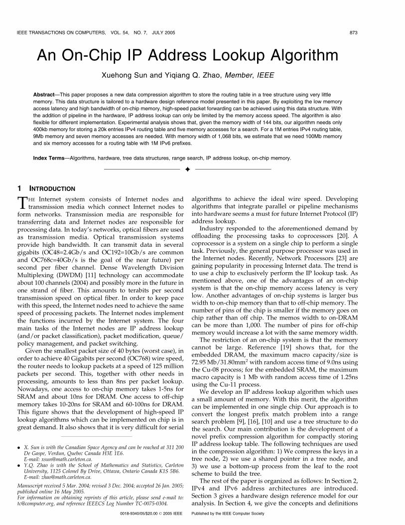
Two distinct prefixes may share at most one endpoint.For example, in Table 1, prefix 001* has endpoints 8 and 16and prefix 01* has endpoints 16 and 32. They share the sameendpoint 16. Since each prefix can be converted to twoendpoints, N prefixes can be converted to at most2N different endpoints. Fig. 2 is the mapping of prefixesin Table 1 to endpoints and ranges. Notice that 14 prefixesproduce 17 endpoints in this example.

If two consecutive ranges have the same port, the sharedendpoint can be eliminated. Hence, the two ranges can bemerged into one range. For example, since range ½34; 36Þand range ½36; 40Þ both map to port A, we can merge theminto the range ½34; 40Þ. We can assign a unique port to eachrange according to the rule of longest prefix match. We canuse an endpoint to represent the range to its right and, thus,assign the port of the range to the left endpoint. Forexample, let a be an endpoint and b its successor. If port A isassigned to a, it means any address that is in ½a; bÞ ismapped to port A. The algorithm to convert the routingtable into (endpoint, port) tuples is given in the Appendix.Notice that, for simplicity, this algorithm does not do thepossible merge of endpoints mentioned above. In fact, thiscan be easily done by using a variable to record the portassigned to the previous endpoint. Whenever there is a portassignment, we check the port with the recorded port. Ifthey are equal, this endpoint will be eliminated; otherwise,assign the port as usual. Fig. 3 is the result of the conversion

SUN AND ZHAO: AN ON-CHIP IP ADDRESS LOOKUP ALGORITHM 875

Fig. 1. Hardware design reference model.

TABLE 1A Mini Routing (Maximum Prefix Length = 6)

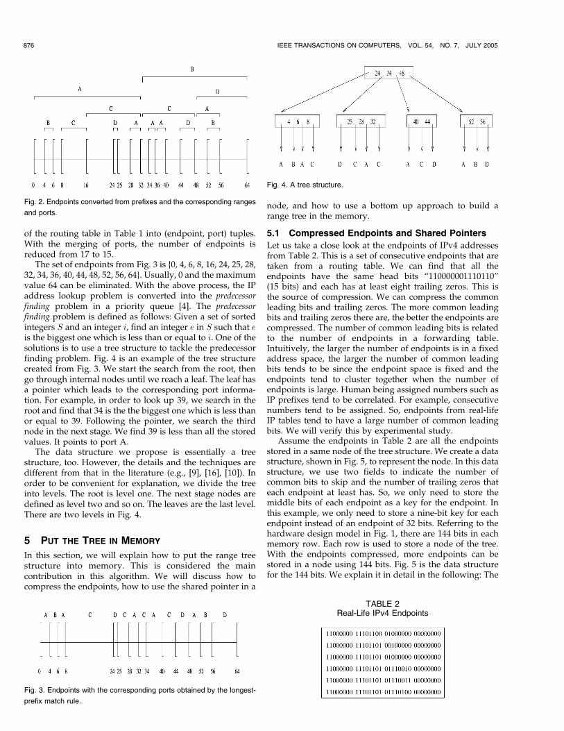
of the routing table in Table 1 into (endpoint, port) tuples.With the merging of ports, the number of endpoints isreduced from 17 to 15.

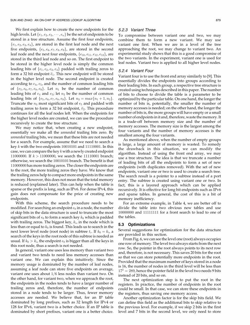
The set of endpoints from Fig. 3 is {0, 4, 6, 8, 16, 24, 25, 28,32, 34, 36, 40, 44, 48, 52, 56, 64}. Usually, 0 and the maximumvalue 64 can be eliminated. With the above process, the IPaddress lookup problem is converted into the predecessorfinding problem in a priority queue [4]. The predecessorfinding problem is defined as follows: Given a set of sortedintegers S and an integer i, find an integer e in S such that eis the biggest one which is less than or equal to i. One of thesolutions is to use a tree structure to tackle the predecessorfinding problem. Fig. 4 is an example of the tree structurecreated from Fig. 3. We start the search from the root, thengo through internal nodes until we reach a leaf. The leaf hasa pointer which leads to the corresponding port informa-tion. For example, in order to look up 39, we search in theroot and find that 34 is the the biggest one which is less thanor equal to 39. Following the pointer, we search the thirdnode in the next stage. We find 39 is less than all the storedvalues. It points to port A.

The data structure we propose is essentially a treestructure, too. However, the details and the techniques aredifferent from that in the literature (e.g., [9], [16], [10]). Inorder to be convenient for explanation, we divide the treeinto levels. The root is level one. The next stage nodes aredefined as level two and so on. The leaves are the last level.There are two levels in Fig. 4.

5 PUT THE TREE IN MEMORY

In this section, we will explain how to put the range treestructure into memory. This is considered the maincontribution in this algorithm. We will discuss how tocompress the endpoints, how to use the shared pointer in a

node, and how to use a bottom up approach to build arange tree in the memory.

5.1 Compressed Endpoints and Shared Pointers

Let us take a close look at the endpoints of IPv4 addressesfrom Table 2. This is a set of consecutive endpoints that aretaken from a routing table. We can find that all theendpoints have the same head bits “110000001110110”(15 bits) and each has at least eight trailing zeros. This isthe source of compression. We can compress the commonleading bits and trailing zeros. The more common leadingbits and trailing zeros there are, the better the endpoints arecompressed. The number of common leading bits is relatedto the number of endpoints in a forwarding table.Intuitively, the larger the number of endpoints is in a fixedaddress space, the larger the number of common leadingbits tends to be since the endpoint space is fixed and theendpoints tend to cluster together when the number ofendpoints is large. Human being assigned numbers such asIP prefixes tend to be correlated. For example, consecutivenumbers tend to be assigned. So, endpoints from real-lifeIP tables tend to have a large number of common leadingbits. We will verify this by experimental study.

Assume the endpoints in Table 2 are all the endpointsstored in a same node of the tree structure. We create a datastructure, shown in Fig. 5, to represent the node. In this datastructure, we use two fields to indicate the number ofcommon bits to skip and the number of trailing zeros thateach endpoint at least has. So, we only need to store themiddle bits of each endpoint as a key for the endpoint. Inthis example, we only need to store a nine-bit key for eachendpoint instead of an endpoint of 32 bits. Referring to thehardware design model in Fig. 1, there are 144 bits in eachmemory row. Each row is used to store a node of the tree.With the endpoints compressed, more endpoints can bestored in a node using 144 bits. Fig. 5 is the data structurefor the 144 bits. We explain it in detail in the following: The


Fig. 2. Endpoints converted from prefixes and the corresponding ranges

and ports.

Fig. 3. Endpoints with the corresponding ports obtained by the longest-

prefix match rule.

Fig. 4. A tree structure.

TABLE 2Real-Life IPv4 Endpoints

data structure has six fields. The first field is a one-bit fieldto indicate whether the node is an internal node or a leafnode. The second field is the number of endpoints stored inthis node. If the number of endpoints stored in any nodedoes not exceed 16, then 4 bits are needed for this field. Thethird field records the number of head bits to skip in theIP address (endpoint) and the fourth field is the number ofzeros to ignore at the trail of the IP address (endpoint). Ingeneral, for IPv4 addresses, these two fields need at mostfive bits each. For IPv6 addresses, these two fields need atmost seven bits each. We will further discuss how to reducethe number of bits for these fields in later sections. The nextfield is for the keys. The last field is the pointer indexing tonext level nodeof the tree structure.Weuse 20bits in this fieldfor supporting 500k entry forwarding tables. This is becauseeach entry can produce at most two endpoints and eachendpoint has its corresponding port information. Thus, theexternal SRAM which stores port information can have asmanyas1Mentries in theworst case,which canbe indexedby20 bits. To sum up, for IPv4, the first four fields and the lastfield use 1 + 4 + 5 + 5 + 20 = 35 bits. The leftover 109 bits areused to store asmany keys as possible. For IPv6, the first fourfields and the last field use 1 + 4 + 7 + 7 + 20 = 39 bits. Theleftover 105 bits are used to store as many keys as possible.The order of the fields is not important. This is the basicstructure, but it can be modified for different variants. Forexample, the first field may be removed if possible. Thepointer fieldmust be at least 22 bits long ifwewant to support2M entry forwarding tables. We will mention later that thepointer field in a different level nodemay have different bits.The 144 bits can be varied.

We may notice that each node has only one pointerrather than many pointers, as in the case shown in Fig. 4.This is where our shared pointer goes. This scheme savesmemory tremendously. As defined in the previous section,the tree is divided into levels. The nodes in each level arestored in ordered consecutive rows, such as in Fig. 6. In thisway, all the endpoints in a node can share one pointer. Theexact pointer of a subtree can be determined by the positionof the corresponding endpoint. For example, assume a nodewith sorted endpoints p1; p2; p3; p4. Traditionally, we wouldneed five pointers. Here, we only need the pointer thatpoints to the node whose endpoints are smaller than p1.Since other nodes are stored in ordered consecutive rows,we can find the node of a search by knowing the position ofthe destination address in the searched node. For example,if the searched destination address is greater than or equalto p3 but less than p4, we can find the node by adding 3 tothe stored pointer.

The search of the keys in a node is carried out in theregisters (or using logic circuit). It is very fast compared tomemory access. Also, the time can be overlapped withmemory access. We can also use a binary search in the keysof a node to speed up the search in the registers.

Two functions are needed for endpoints compression:One is for calculating the number of the common leadingbits of a group of endpoints and another is for calculating

the common trailing zeros of the group. For calculating thenumber of common leading bits of the group, we only needto calculate the number of common leading bits of thesmallest and the biggest endpoints in the group. Thenumber of common trailing zeros can be calculatediteratively as follows: The trailing zeros of the first endpointare counted and recorded as the candidate number ofcommon trailing zeros. Then, the trailing zeros of the nextendpoint are counted. If the number of the trailing zeros ofthe next endpoint is smaller than the candidate number, thecandidate number is changed to the smaller one; otherwise,the candidate number is unchanged. This operation isperformed for the left endpoints until we exhaust all theendpoints. Using this approach to find the number ofcommon trailing zeros of n endpoints, OðnÞ operations areneeded. Oð2Þ operations are needed to find the number ofcommon leading bits of any sorted group. This can also bedone by ORing together all the bits of the endpoint and thencounting trailing zeros (which is probably more efficient,both in hardware and software).

5.2 Build the Tree from the Bottom Up

Given a set of sorted endpoints, we next discuss how tocreate a tree structure from it. We adopt a bottom-upapproach. First, we assign endpoints to leaf nodes and thento the next highest level until the root level. Beginning withthe smallest value endpoint, we try to store as manyendpoints to a node as possible. We use IPv4 for theexplanation in the following. From the analysis of theprevious subsection, we know that there are 109 bits to storethe compressed keys. Since each endpoint is 32 bits long, wecan store at least three endpoints (3 � 32 ¼ 96 < 109) evenwithout key compression. Therefore, we initially select thefirst four endpoints as a group and calculate the total bits ofthe compressed keys. If the total bits is bigger than 109, thenwe cannot store these four keys. Instead, we store the first


Fig. 5. The row data structure for a node of the tree.

Fig. 6. Tree in memory.

three keys. If the total bits is equal to 109, we store thesefour keys. Otherwise, if the total bits is smaller than 109, wehave the potential to store more keys. Thus, we need toprobe further. We add the next endpoint to the group andrepeat the above procedure. In this way, we can learn howmany keys can be stored in the 109 bits.

Several variants are proposed in the following todescribe the details of the tree creation. Specifically, theydiffer in how to calculate the compressed keys and selectendpoints to store in the higher level nodes. They representsome trade-offs between the memory size and the numberof memory accesses.

5.2.1 Variant One

Let fe1; e2; e3; � � � ; eng be the set of endpoints to be stored ina tree structure. Assume that the first four endpoints,fe1; e2; e3; e4g, are stored in the first leaf node, then theendpoint fe5g will be stored in the next higher level node.Assume the next five endpoints, fe6; e7; e8; e9; e10g, arestored in the second leaf node, then the endpoint fe11g willbe stored in the next higher level node and so on.

For this scheme, the endpoint(s) in the next higher levelnode must be involved in the leaf nodes to calculate thecompressed keys. Specifically, in the aforementionedexample, two endpoints, fe1g and fe5g, are involved tofind the the common leading bits of the first leaf node;fe1; e2; e3; e4g are used to find the common trailing zeros ofthe first leaf node. Two endpoints, fe5g and fe11g, areinvolved to find the common leading bits of the second leafnode; fe6; e7; e8; e9; e10g are used to find the commontrailing zeros of the second leaf node; and so on. Next,we will explain why the higher level endpoints will beinvolved in the calculation of compressed keys using aconcrete example.

For example, in Table 3 (the blank between bits is forconvenience of reading), the first seven endpoints are storedin the first leaf node. The next endpoint, “1000011011101111 00001101 10000000,” will be stored in a higherlevel node. The next four endpoints following “1000011011101111 00001101 10000000” will be stored in the next leafnode. “11111000 11110000 00010000 11000000” will bestored in a higher level node and so on.

The common leading bits of the first leaf node are“10000” instead of “1000000011.” The number of commontrailing zeros is eight. The common leading bits of thesecond leaf node are “1” (because “10000110 1110111100001101 10000000” and “11111000 11110000 0001000011000000” are involved to calculate the common leadingbits) instead of “1101.” The number of common trailingzeros is eight.

The reason is as follows: Let us assume that we aresearching endpoint “10011111 11111111 1111111100000000.” This endpoint is greater than the endpoint“10000110 11101111 00001101 10000000” and less than thefirst endpoint in the second group. If we took “1101” as theleading bits of the second group, i.e., we skipped four bits,we would mistake “10011111 11111111 11111111 00000000”as greater than the last endpoint in the second group.

After constructing the leaf nodes, we proceed to the nextlevel using the same method. The number of endpoints inthis level are reduced to approximately N=k, where N is the

number of endpoints in the leaf level and k is the averagenumber of endpoints in a leaf node.

As we can see, the cost for constructing the tree structureis not high. Let N be the total number of endpoints. Sortingthe endpoints may take OðN logNÞ time. However, after thefirst sorting, we can incrementally add or delete anendpoint, which takes only OðNÞ time using binary search.Assigning ports to endpoints takes OðNÞ time. Creating thenodes takes OðNÞ time. Putting them together, we needOðNÞ time to create the tree structure.

The preferred architecture for a router is to use twobanks of memory for IP packet forwarding. One bank is forupdating and the other is for searching. One advantage ofthis architecture is that the updating will not interfere withthe searching. With this architecture, an update can beperformed in less than one second. This architecture is evencomparable to some dynamic data structures in terms ofmemory utilization. For example, the memory utilization ofa basic B-tree [1] is 50 percent in the worst case, which is thesame as the two-banks-of-memory architecture. For a veryfast update, say more than 10k updates per second, we neednew techniques. This will be studied in our future work.

A word for IPv6: If the endpoints of an IPv6 addresscannot be compressed, we cannot store even one address ina row. This is because an IPv6 address is 128 bits long andthe key field of our data structure is only 105 bits. In thiscase, we may allow two rows to store the key with a minormodification of the data structure. IPv6 addresses may haveconsecutive zeros in the middle rather than in the trail. Wemay compress these zeros. However, we do not haveenough IPv6 routing tables for the experiment, and we willnot go into details. Nonetheless, experiments on small IPv6routing tables are presented in this paper for the unmodi-fied data structure.

5.2.2 Variant Two

The essential difference between variants one and two isthat a new endpoint is created to store in the higher levelnode rather than an existing endpoint. We describe thealgorithm first, then explain the reason to do so.


TABLE 3Calculating the “Common Leading Bits”

We first explain how to create the new endpoints for the

high levels. Let fe1; e2; e3; � � � ; eng be the set of endpoints to bestored in a tree structure. Assume the first four endpoints,

fe1; e2; e3; e4g, are stored in the first leaf node and the next

five endpoints, fe5; e6; e7; e8; e9g, are stored in the second

leaf node and the next four endpoints, fe10; e11; e12; e13g, arestored in the third leaf node and so on. The first endpoint to

be stored in the higher level node is simply the common

leading bits of fe1; e2; e3; e4g padded with trailing zeros to

form a 32 bit endpoint e1. This new endpoint will be stored

in the higher level node. The second endpoint is created

according to e4, e5, and the number of common leading bits

of fe5; e6; e7; e8; e9g. Let n1 be the number of common

leading bits of e4 and e5; let n2 be the number of common

leading bits of fe5; e6; e7; e8; e9g. Let n3 ¼ maxfn1 þ 1; n2g.Truncate the n3 most significant bits of e5 and padded with

trailing zeros to form a 32 bit endpoint, e2. This procedure

continues for all the leaf nodes left. When the endpoints for

the higher level nodes are created, we can use the procedure

recursively to create the tree structure.We may notice that, when creating a new endpoint,

essentially we make all the unneeded trailing bits zero. Byunneeded trailing bits, we mean that these bits are not neededfor a search. For example, assume that we need to search akey kwith the two endpoints 10010101 and 11110001. In thiscase,we can compare thekey kwith anewly created endpoint11000000. If k > 11000000, we search the 11110001 branch;otherwise, we search the 10010101 branch. The benefit is that11000000hasmore trailing zeros. The closer the endpoints areto the root, the more trailing zeros they have. We know thatthe trailing zeros help to compactmore endpoints in the samememory. However, this does notmean that the total memoryis reduced (explained later). This can help when the table issparse or the prefix is long, such as IPv6. For dense IPv4, thisgain does not compensate for the price of creating newendpoints.

With this scheme, the search procedure needs to bemodified. For searching an endpoint e0 in a node, the numberof skip bits in the data structure is used to truncate the mostsignificant bits of e0 to form a search key k0 which is paddedwith trailing zeros. The biggest key, ki, in the node which isless than or equal to k0 is found. This leads us to search in thenext lower level node (root node) in subtree ti. If k0 ¼ ki, asearch of the keys in the root node of this subtree is needed asusual. If k0 > ki, the endpoint e0 is bigger than all the keys inthis root node, thus a search is not needed.

In general, variant one uses less memory than variant twoand variant two tends to need less memory accesses thanvariant one. We can explain this intuitively. Since thememory usage is dominated by the number of leaf nodes,assuming a leaf node can store five endpoints on average,variant one uses about 1=6 less nodes than variant two. Onthe other hand, for variant two, when we approach the root,the endpoints in the nodes tends to have a larger number oftrailing zeros and, therefore, the number of endpointsstored in a node tends to be larger. Thus, fewer memoryaccesses are needed. We believe that, for an IP tabledominated by long prefixes, such as 32 length for IPv4 or128 for IPv6, variant two is a better choice. If an IP table isdominated by short prefixes, variant one is a better choice.

5.2.3 Variant Three

To compromise between variant one and two, we maycombine them to form a new variant. We may usevariant one first. When we are in a level of the treeapproaching the root, we may change to variant two. Anexperimental study shows that this is a good compromise ofthe two variants. In the experiment, variant one is used forleaf nodes. Variant two is applied to all higher level nodes.

5.2.4 Variant Four

Variant four is to use the front end array similarly to [9]. Thisessentially divides the endpoints into groups according totheir leading bits. In each group, a respective tree structure iscreatedusing techniquesdescribed in this paper. Thenumberof bits to choose to divide the table is a parameter to beoptimizedby the particular table.On onehand, the longer thenumber of bits is, potentially, the smaller the number ofmemory accesses is needed; on the other hand, the longer thenumber of bits is, themore groupswill have empty or a smallnumberof endpoints in it and, therefore,waste thememory. Itis a trade-off between memory size and the number ofmemory accesses. The memory size is the largest among thefour variants and the number of memory accesses is thesmallest among the four variants.

As mentioned above, when the number of empty groupsis large, a large amount of memory is wasted. To remedythe drawback in this situation, we can modify thealgorithm. Instead of using the front end array, we mayuse a tree structure. The idea is that we truncate a numberof leading bits of all the endpoints to form a set of newendpoints (with duplicates removed). With the set of newendpoints, variant one or two is used to create a search tree.The search result is a pointer to a subtree instead of a portentry. The subtree is created using variant one or two. Infact, this is a layered approach which can be appliedrecursively. It is effective for long bit endpoints such as IPv6and sparse tables. In general, the cost of this is a bit ofmemory inefficiency.

For an extreme example, in Table 4, we are better off todivide the table into two obvious new tables and use10000000 and 11111111 for a front search to lead to one ofthe tables.

5.3 Optimizations

Several suggestions for optimization for the data structureare provided in this section.

FromFig. 6,we can see the level one (root) always occupiesone rowofmemory. The level two always starts from the nextrow. So, the pointer in the root always points to its next rowand, therefore, is not necessary. This saves 20 bits for the rootso that we can store potentially more endpoints in the root.Provided that themaximumnumber of keys stored in a nodeis 16, the number of nodes in the third level will be less than172 ¼ 289, hence the pointer field in the level two needs 9 bitsinstead of 20 bits, and so on.

The next optimization step is to put the root in theregisters. In practice, the number of endpoints in the rootcould be small. In that case, we can store these endpoints inthe registers, thus saving one memory access.

Another optimization factor is for the skip bits field. Wecan define this field as the additional bits to skip relative tothe previous level. For example, if we skip 2 bits in the firstlevel and 7 bits in the second level, we only need to store


7� 2 ¼ 5 as additional bits to skip. From the experiments,3 bits is enough for IPv4.

6 EXPERIMENTAL STUDY

We download IPv4 routing tables from [21], [18] and IPv6routing tables from [22] for the experiments. They are thebasis for our experiments study. We plan three groups ofthe experiments. One is to use the original tables. Another isto create new tables by expanding original tables. The thirdone is to generate random tables. Results are analyzed in thefollowing subsections.

6.1 Port Merge

If two consecutive intervals have the same port, the twoconsecutive intervals can be merged into one interval. Thisreduces the number of endpoints. Table 5 shows the portmerge effect for IPv4 addresses. The nonmerge rate is equalto the number of endpoints with merge divided by thenumber of endpoints without merge. From the table, we cansee that the merge effect is very significant. For example, forpacbell, the nonmerge rate is 57 percent. This implies thatwe can save about 43 percent memory if the merge effect istaken into account. We also conduct experiments byrandomly assigning port numbers to prefix. The mergeeffect is not significant. This indicates that, in real-life tables,the port assignment has some correlation between neigh-boring intervals. By observing the port numbers in a real-life forwarding table, we can see the port numbers tend tobe clustered. For IPv6, due to the lack of large real-lifetables, we cannot analyze the effect. In the followingexperiments, we will not perform port merge for the setof endpoints.

6.2 Comparisons on Variants

Table 6 gives a general picture of the performance of thefour variants. It shows the memory requirement and thenumber of memory accesses for the original tables underdifferent variants. Columns with headings one, two, andthree correspond to variants one, two, and three. Thecolumn with heading four is the result of variant four with 6as the number of the front end bits. The column with

heading five is the result of variant four with 14 as thenumber of the front end bits. We can see variant one usesthe smallest amount of memory, but the number of memoryaccesses is the highest. Variant three is well balanced. Otherexperiments we conducted show similar results with oneexception, that, when a table is dominated by short prefixes,variant one shows the best performance for both memorysize and accesses. In order to avoid swamping pages due tohuge experimental results, we choose variant three for thefollowing experiments.

6.3 Results Using Real-Life Tables

This section shows the results using real-life tables. We firstdescribe the characteristics of the forwarding tables. Theseven IPv4 tables are dominated by 24 bit prefixes of morethan 50 percent. The next largest number of prefixes are 23,22, 19, 32, and 16 bits. The IPv6 tables are dominated by 48,35, 28, and 24 bits of length. Some tables have as high as70 percent 48 bit prefixes.

Table 7 is the result of IPv4 using variant three. The firstcolumn is the name for network access points (NAPs). Thesecond column is the number of entries (prefixes) in therouting tables. The third column is the ME ratio. TheME ratio is defined as the number from dividing thememory requirement in bits by the number of prefixes. Itmeasures the average number of bits needed for one prefix.The table shows that about 22 bits are needed for a prefix.Note that, if the port merge is taken into account, fewer bitsare needed.

The Arity of a node is defined as the number of subtreesof the node. The average arity measures the averagenumber of subtrees of all the nodes in the tree. The lastcolumn is the average arity from each routing table. Fromthe average arity, we can roughly estimate the performanceof a routing table with a different size. For example,assuming the average arity of 8, a routing table with1M prefixes will need roughly log8 1000000 � 7 memoryaccesses.

The above results are obtained without using anyoptimizations mentioned in the previous section. Weshould mention that our data structure is also suitable fora pipeline implementation. In that case, the lookup speed isonly restricted by the memory access latency.

Table 8 is the result of IPv6 using variant three. We use168 bits memory width so that the key field is 128 bits long,which can accommodate at least one IPv6 endpoint. Thelow ME ratio (about 30) for t3 and t4 is probably due to ahigh percentage (above 70 percent) of length 48 prefixes. Forother tables, no prefix has a percentage above 40 percent.


TABLE 4An Example

TABLE 5Port Merge Effect

6.4 Results Using the Expanded IPv4 Tables

This section provides results for tables expanded from real-life tables. The six real-life IPv4 tables are combined and theduplicates are removed to form a large table as a basis. Thesize of the resulting table is 50,449. We can expand the basistable to a larger size table. The method of expanding thetable is to pick a prefix of length 24 and expand it to 28 ¼256 prefixes of length 32. Given a size of a table we want toexpand and the total number of prefixes of length 24, wecan roughly figure what percentage of the prefixes oflength 24 needs to be expanded. Then, we randomly selectthis percentage of prefixes of length 24 to expand. Usingthis method, we generated five tables of sizes of 66,004,128,479, 258,784, 591,050, and 939,889. We have doneexperiments with different memory widths. We make thelength of the key field in a node 32, 64, 128, 256, 512, or1,024 bits. Assuming that the total length of the other fieldsis 36 bits for IPv4, the memory width comes to 68, 100, 164,292, 548, or 1,060 bits, respectively. Table 9 shows thememory size as a function of table size and memory width.The result is also plotted in Fig. 7. From the results,we can seethat 164 bits and 292 bits memory width are better choicesthan other memory widths for this set of tables. We can alsosee that the memory requirement increases proportionally tothe increase of the number of prefixes, but at a small speed.For example, using a 164 bit memory width, the ME ratio isabout 19.4 for tables of size around 50k; the ME ratio is onlyabout 9.5 for tables of size around 1M.

The number of memory accesses is shown in Table 10.We can see it is not sensitive to the size of the tables. Itindicates that our algorithm scales well to the size of theforwarding table.

6.5 Results Using the Expanded IPv6 Tables

Since we do not have large IPv6 tables, we randomlygenerate the tables and then expand them. The method is asfollows: First, we randomly generate a table of size 10k withabout 80 percent of prefix length 48 and lengths from 12 to64 are uniformly distributed. A second table of size 10k isgenerated in the same way with about 80 percent of prefixlength 64 instead of 48. Then, the two tables are combinedwith duplicates removed. This is the basis table forexpansion which has about 40 percent of prefixes oflength 48 and 64 each. When expanding, a prefix withlength 64 is randomly selected and expanded to a numberof prefixes of length 128. The exact number is randomlychosen between 128 and 1,024. The bits that expand frombit 65 to bit 128 are also randomly generated. Expansioncontinues until we reach the desired size of the table.

Using this scheme, we generated seven tables of sizes of20,000, 31,284, 48,210, 144,124, 223,112, 530,601, and1,208,666. The memory widths for this set of experimentsare 168, 296, 552, and 1,064, respectively. Assuming that thetotal length of other fields is 40 bits for IPv6, the length ofthe key field in a node is 128, 256, 512, and 1,024,respectively. Shorter memory widths cannot accommodatea single IPv6 endpoint in the worst case and modificationneeds to be done.


TABLE 7Results of IPv4 Using 144 Bits Memory Width

TABLE 6Experiments with IPv4 Using 144 Bits Memory Width

TABLE 8Results of IPv6 Using 168 Bits Memory Width

Table 11 shows the memory size as a function of tablesize and memory width. The result is plotted in Fig. 8. Fromthe results, we can see 1,064 bits memory width is the bestchoice among all memory widths for this set of tables. Wecan also see that the memory requirement increasesproportionally to the increase of the number of prefixes.The ME ratio does not change much when the number ofprefixes increases. For example, the ME ratio is 115.8 fortables of size of around 20k and 125.6 for tables of size ofaround 1M if the memory width is 1,064. All ME ratios arerather high compared with the small real-life tables. Thereason for this is that the endpoints in real-life tables arecorrelated. The endpoints in randomly generated tables arenot. For example, when a 64 bit prefix expands to 128, thetrailing 64 bits are randomly generated. If we select 128 to1,024 entries from a space of size of 264, it is rare that anytwo of them correlate. (We borrow the word correlate to

roughly express the following idea: For example, we cansay 11111100 and 11111111 correlate, but 10100100 and11111111 not so much).

The number of memory accesses is shown in Table 12.Similarly to IPv4, it is not sensitive to the size of the tables.

7 PREVIOUS WORK

Papers on address lookup algorithms are abound in theliterature. It is not possible to mention all of them. We onlycompare with those that are similar to our approach. Wealso list papers that use a small amount of memory andomit those that use a large amount of memory. Surveys onaddress lookup algorithms were given in [14], [13].Performance measurements for some of the algorithms arehighlighted and compared as follows: Multiway search [9],[16] is the most similar approach to our method. However,


TABLE 9Memory Size for IPv4 as a Function of Table Size and Memory Width

Fig. 7. Memory size for IPv4 as a function of table size with different memory widths.

due to the lack of techniques to compress and optimize the

data structures, larger memory requirements than ours are

reported and the number of memory accesses is comparable

to ours. Using a 32 byte cache line (which equals 256 bits

memory width), a 6-way search can be done. For a routing

table with over 32,000 entries, 5.6M bits memory is needed.

In the worst case, four memory accesses are needed. If

256 bit memory width is used, we can report much better

results than those in the previous section. Even with 144 bit

memory width, we reported more favorable results than

those from [9].Reference [17] proposed an algorithm which requires a

worst case of logW hash lookups, where W is the length of

the address in bits. Hence, at most five hash lookups for

IPv4 and at most seven hash lookups for IPv6 are needed.

However, data from [9] showed that this algorithm needs

1,600K bytes for an IPv4 routing table with roughly

40k entries. In addition to that, the building of the data

structure is not fast.Reference [7] uses LC-trie for storing the table. They

reported that about 4M bits are needed for the LC-trie.

According to the paper, they need at least 100 bits for each

prefix.Reference [8] presented an IP address lookup scheme

and a hardware architecture. The routing table is meant to

put in off-chip memory, for they need 450-470k bytes

memory for a routing table with 40,000 entries. They


TABLE 10Number of Memory Accesses for IPv4

as a Function of Table Size and Memory Width

TABLE 11Memory Size for IPv6 as a Function of Table Size and Memory Width

Fig. 8. Memory size for IPv6 as a function of table size with different memory widths.

reported one to three memory accesses. They comparedtheir scheme favorably with those proposed in [3] and [5].

Reference [15] was also aimed at hardware implementa-tion. They used a compact stride multibit trie data structureto search the prefixes. They reported 4.3MB memory for aforwarding table of 104,547 entries. The algorithm allowsfor incremental updates, but is not scalable to IPv6.

Although [10] achieves OðlognÞ complexity for bothupdate and search, the memory required is much largerthan ours.

Table 13 shows roughly the bits consumed for eachIPv4 prefix in the above-mentioned papers. These figuresare derived from the experimental reports from each paper.They just provide a general picture, rather than an accuratemeasure, because data used for experiments, data struc-tures, and resource assumption, etc., are different for eachpaper. For example, reference [15] used 19 bits for the nexthop index field and we use 22 bits.

There are several papers, e.g., [9], [17], that deal withIPv6 address lookup. They have different merits fromdifferent perspective views of performance. Our algorithmhas the advantage of using the lowest memory and thesearch speed is comparable to others.

8 CONCLUSION

We developed a novel algorithm which is tailored tohardware technology. The distinguishing merit of ouralgorithm is that it has a very small memory requirement.With this merit, a routing table can be put into a single chip,thus, the memory latency to access the routing table can bereduced. With the pipeline implementation of our algo-rithm, the IP address lookup speed can only be limited bythe memory access technology.

Experiment analysis shows that, given the memorywidth of 144 bits, our algorithm needs only 400kb memoryfor storing a 20k entry IPv4 routing table and five memoryaccesses for a search. For a 1M entry IPv4 routing table, 9Mbmemory and seven memory accesses are needed. With amemory width of 1,068 bits, we estimate that we need100Mb of memory and six memory accesses for a routingtable with 1M IPv6 prefixes.

Real-life tables have some structures. Modifying ouralgorithm to exploit these structures can achieve betterperformance.

APPENDIX

AN ALGORITHM FOR CONVERTING THE PREFIXES TO

ENDPOINTS

Step 1: Sort the prefixes.The host part of a prefix is filled with 0s and the prefix is

treated as an integer. Prefixes are sorted according to the

value of the integer. The smaller value prefix is sorted in the

front. If two prefixes have the same value, the one whose

length is smaller is sorted in the front.Step 2: Assign ports to endpoints.We have a stack. Let “max” be the maximum integer

(endpoint) in the address space, “def” the default port for

the address space, “M” the variable for the endpoint, and

“N” the variable for the port.

N=def;

M=max;

push N;

push M;

For each prefix P=[b, e) with port p

in the sorted routing table {

pop M;

If (b<M) {

assign p to b;

push M; (push back M.)

push p;

push e;

} else if (b=M) {

assign p to b;

while (b=M) {

pop N;

pop M;

}

push M; (M>b so push back.)

push p;

push e;

} else if (b>M) {

oldM=M;

while (b>M) {

pop N;

if (oldM not = M) {

(assign oldM’port to M.)


TABLE 12Number of Memory Accesses for IPv6 as a Function of Table Size and Memory Width

TABLE 13Bits Consumed for Each IPv4 Prefix

pop M;

pop N; (get the next port.)

assign port N to oldM;

push N;

push M; (push back N, M.)

}

oldM=M;

pop M;

}

while (b=M) {

pop N;

pop M;

}

push M; (M>b so push back.)

push p;

push e;

}

ACKNOWLEDGMENTS

The authors would like to acknowledge Greg Soprovich of

SiberCore Technologies for providing comments and

suggestions for most of the experimental scenarios. A

patent was filed based on this work.

REFERENCES

[1] R. Bayer and E. McCreight, “Organization and Maintenance ofLarge Ordered Indexes,” Acta Informatica, vol. 1, no. 3, pp. 173-189,Sept. 1972.

[2] S. Deering and R. Hinden, “Internet Protocol, Version 6 (IPv6)Specification,” RFC 2460, Dec. 1998.

[3] M. Degermark, A. Brodnik, S. Carlsson, and S. Pink, “SmallForwarding Tables for Fast Routing Lookups,” Proc. ACMSIGCOMM, pp. 3-14, Sept. 1997.

[4] P. van Emde Boas, R. Kaas, and E. Zijlstra, “Design andImplementation of an Efficient Priority Queue,” Math. SystemsTheory, vol. 10, pp. 99-127, 1977.

[5] P. Gupta, S. Lin, and N. McKeown, “Routing Lookups inHardware at Memory Access Speeds,” Proc. Infocom, Apr. 1998.

[6] R. Hinden and S. Deering, “Internet Protocol Version 6 (IPv6)Addressing Architecture,” RFC 3513, Apr. 2003.

[7] S. Nilsson and G. Karlsson, “IP Address Lookup Using LC-Tries,”IEEE J. Selected Areas in Comm., vol. 17, no. 6, pp. 1083-1092, June1999.

[8] N.-F. Huang and S.-M. Zhao, “A Novel IP-Routing LookupScheme and Hardware Architecture for Multigigabit SwitchingRouters,” IEEE J. Selected Areas in Comm., vol. 17, no. 6, pp. 1093-1104, June 1999.

[9] B. Lampson, V. Srinivasan, and G. Varghese, “IP Lookups UsingMultiway and Multicolumn Search,” IEEE/ACM Trans. Network-ing, vol. 7, pp. 324-334, 1999.

[10] H. Lu and S. Sahni, “O(log n) Dynamic Router-Tables for Ranges,”Proc. IEEE Symp. Computers and Comm., pp. 91-96, 2003.

[11] R. Ramaswami and K.N. Sivarajan, Optical Networks: A PracticalPerspective. San Francisco: Morgan Kaufmann, 1998.

[12] Y. Rekhter and T. Li, “An Architecture for IP Address Allocationwith CIDR,” RFC 1518, Sept. 1993.

[13] M.A. Ruiz-Sanchez, E.W. Biersack, and W. Dabbous, “Survey andTaxonomy of IP Address Lookup Algorithms,” IEEE Network,vol. 15, no. 2, pp. 8-23, Mar./Apr. 2001.

[14] S. Sahni, K. Kim, and H. Lu, “Data Structures for One-Dimensional Packet Classification Using Most-Specific-RuleMatching,” Int’l J. Foundations of Computer Science, vol. 14, no. 3,pp. 337-358, 2003.

[15] K. Seppanen, “Novel IP Address Lookup Algorithm for Inexpen-sive Hardware Implementation,” WSEAS Trans. Comm., vol. 1,no. 1, pp. 76-84, 2002.

[16] S. Suri, G. Varghese, and P. Warkhede, “Multiway Range Trees:Scalable IP Lookup with Fast Updates,” Proc. GLOBECOM, 2001.

[17] M. Waldvogel, G. Varghese, J. Turner, and B. Plattner, “ScalableHigh Speed IP Routing Lookups,” Proc. ACM SIGCOMM, pp. 25-36, Sept. 1997.

[18] http://bgp.potaroo.net/, 2003.[19] http://www-3.ibm.com/chips/products/asics/products/

ememory.html, 2003.[20] http://www.linleygroup.com/, 2005.[21] http://www.merit.edu/ipma/routing_table/, 2003.[22] http://www.mcvax.org/~jhma/routing/ipv6/, 2005.[23] http://www.npforum.org/org/, 2005.

Xuehong Sun received the PhD degree fromCarleton University, Canada. He is a visitingfellow at the Canadian Space Agency and amember of AIAA. He is a cofounder of SourithmCorp., which commercializes technologiesthrough advanced algorithms for Internet Proto-col (IP) address lookup and packet classificationin Internet routers.

Yiqiang Q. Zhao (M’01) received the PhDdegree from the University of Saskatchewan in1990. After a two-year appointment as a post-doctoral fellow sponsored by the CanadianInstitute for Telecommunications Research(CITR) at Queen’s University, he joined theDepartment of Mathematics and Statistics of theUniversity of Winnipeg as an assistant professorin 1992 and became an associate professor in1996. In 2000, he moved to Carleton University,

where he is now a full professor and the director of the School ofMathematics and Statistics. His research interests are in appliedprobability and stochastic processes, with particular emphasis oncomputer and telecommunication network and inventory controlapplications. He has published approximately 50 papers in refereedjournals, delivered approximately 50 talks at conferences, and beeninvited more than 30 times to speak to seminars/colloquia or workshops.He has also had considerable experience interacting with industry. Hehas been the recipient of a number of grants from the Natural Sciencesand Engineering Research Council of Canada (NSERC) and industries.He is currently on the editorial board of Operations Research Letters,Queueing Systems, Stochastic Models, and the Journal of Probabilityand Statistical Science. He is a member of the IEEE.

. For more information on this or any other computing topic,please visit our Digital Library at www.computer.org/publications/dlib.


ieee transactions on computers, vol. 54, no. 7, july...

Documents