ieee transactions on automatic control, … · oped an adaptive inverse control scheme for a class...

IEEE TRANSACTIONS ON AUTOMATIC CONTROL, VOL. 50, NO. 6, JUNE 2005 827

Adaptive Identification and Control of Hysteresisin Smart Materials

Xiaobo Tan, Member, IEEE, and John S. Baras, Fellow, IEEE

Abstract—Hysteresis hinders the effective use of smart materialsin sensors and actuators. This paper addresses recursive identifi-cation and adaptive inverse control of hysteresis in smart materialactuators, where hysteresis is modeled by a Preisach operator witha piecewise uniform density function. Two classes of identificationschemes are proposed and compared, one based on the hysteresisoutput, the other based on the time-difference of the output. Con-ditions for parameter convergence are presented in terms of theinput to the Preisach operator. An adaptive inverse control schemeis developed by updating the Preisach operator (and thus its in-verse) with the output-based identification method. The asymptotictracking property of this scheme is established, and for periodicreference trajectories, the parameter convergence behavior is char-acterized. Practical issues in the implementation of the adaptiveidentification and inverse control methods are also investigated.Simulation and experimental results based on a magnetostrictiveactuator are provided to illustrate the proposed approach.

Index Terms—Adaptive control, hysteresis, identification, inver-sion, Preisach operator, smart materials.

I. INTRODUCTION

SMART materials, e.g., magnetostrictives, piezoelectrics,and shape memory alloys (SMAs), show the coupling of

mechanical properties with applied electromagnetic/thermalfields and hence have built-in sensing/actuation capabilities.However, strong hysteresis existing in these materials hinderstheir effective use in sensors and actuators [1]. The hysteresisbehavior often varies slowly with time, which makes the hys-teresis control problem even more challenging. To address thisissue, recursive identification and adaptive control algorithmsare developed in this paper based on a special class of Preisachhysteresis operators.

Hysteresis models can be roughly classified into physics-based models and phenomenological models. An exampleof a physics-based model is the Jiles–Atherton model of fer-romagnetic hysteresis [2], where hysteresis is considered toarise from pinning of domain walls on defect sites. The mostpopular phenomenological hysteresis model used for smartmaterials has been the Preisach operator [3]–[10], where the

Manuscript received November 3, 2004; revised March 10, 2005. Recom-mended by Associate Editor E. Bai. This work was supported by the ArmyResearch Office under the ODDR&E MURI97 Program Grant DAAG55-97-1-0114 to the Center for Dynamics and Control of Smart Structures (through Har-vard University, Cambridge, MA) and by the Lockheed Martin Chair Endow-ment Funds.

X. Tan is with the Department of Electrical and Computer Engi-neering, Michigan State University, East Lansing, MI 48824 USA (e-mail:[email protected]).

J. S. Baras is with the Institute for Systems Research and the Department ofElectrical and Computer Engineering, University of Maryland, College Park,MD 20742 USA (e-mail: [email protected]).

Digital Object Identifier 10.1109/TAC.2005.849215

hysteresis is modeled as a (weighted) aggregate effect of allpossible delayed relay elements, which are parameterized bya pair of threshold variables [11]. A similar type of operator,called Krasnosel’skii–Pokrovskii (KP) operator [12], [13], hasalso been used for modeling hysteresis in smart materials [14],[15]. The difference between the Preisach operator and theKP operator is that delayed relay elements in the latter havefinite slopes. Another phenomenological hysteresis model isthe Prandtl–Ishlinskii (PI) operator [16]. The PI model is asuperposition of elementary play or stop operators, which areparameterized by a single threshold variable [13].

A fundamental approach in coping with hysteresis is inversecompensation, where one aims to cancel out the hysteresiseffect by constructing a right inverse of the hysteresis model(see, e.g., [4], [8]–[10], [15], and [17]–[19]). It has been widelyobserved that hysteretic behaviors of smart materials vary withtime, temperature and some other ambient conditions. Hencethe performance of open-loop inverse compensation based on afixed model is susceptible to model uncertainties. To combat thisproblem, a robust control framework was proposedby combininginverse compensation with control theory [20]. An alternativeapproach is adaptive inverse control [16], [17], [21], where theinverse model is updated adaptively. Tao and Kokotovic devel-oped an adaptive inverse control scheme for a class of hysteresismodels with piecewise linear characteristics cascaded withknown or unknown linear dynamics [17]. Adaptive identificationand inverse control were studied for a discretized KP operatorand applied to an SMA actuator by Webb et al. [21]. Kuhnen andJanocha examined an adaptive inverse scheme for piezoelectricactuators, where the PI hysteresis operator was used [16].

What distinguish this paper from [16], [17], and [21] are: 1)the Preisach operator is used to model the hysteresis nonlinearity;2) the persistent excitation (PE) conditions for parameter conver-gencearepresentedin termsof theinput tothehysteresisoperator;and 3) the asymptotic tracking property of the adaptive inversecontrol algorithm is proved, and for periodic reference trajecto-ries, the parameter convergence behavior is characterized.

For the Preisach operator, the model “parameter” is thePreisach density function. A classical method to identify thedensity function is to twice differentiate the Everett surface ob-tained with first order reversal inputs [11]. Researchers adoptedfunctions of specific forms to fit the Everett surface basedon the least-squares method [4], [7] or fuzzy/neural networkapproximators [10]. Another identification method is to devisethe input carefully and derive the Preisach weighting masses(on a discretization grid) directly from the output measurements(solving for unknowns from equations) [22]. This schemeis very sensitive to measurement noises as one can easily see.

0018-9286/$20.00 © 2005 IEEE

828 IEEE TRANSACTIONS ON AUTOMATIC CONTROL, VOL. 50, NO. 6, JUNE 2005

A third approach is to identify the Preisach weighting massesor the weights for basis functions based on the least-squaresmethod [8], [14], [15], [23]. The aforementioned identificationmethods were all used offline, nonrecursively. In this paper,hysteresis is modeled by a Preisach operator with a densityfunction that is constant within each cell of the discretizationgrid, and the density values are identified recursively. Tworecursive identification algorithms are proposed and compared,one based on the hysteresis output and the other based on thetime-difference of the output.

A necessary condition and a sufficient condition for param-eter convergence are given in terms of the input to the Preisachoperator. In contrast to persistent excitation conditions foridentification of linear systems, which are centered aroundthe number of frequency components of the input signal, theconditions here involve the reversal behavior of the input.For ease of presentation, the analysis is done primarily for aPreisach operator with discrete weighting masses (obtained byassuming the density function within each cell is concentratedas a mass at the cell center). The extension to the case of apiecewise constant density is then briefly outlined.

An adaptive inverse control scheme is developed by updatingthe Preisach model (and thus its inverse) with the output-basedidentification algorithm. It is shown in this paper that, with theadaptive inverse scheme, the tracking error approaches zeroasymptotically. Furthermore, for periodic reference trajectories,the parameter convergence behavior under this scheme can becharacterized if the reference trajectory visits the positive ornegative saturation value. On the other hand, it is shown thatadaptive inverse control using the difference-based algorithmfor parameter update cannot achieve asymptotic tracking.These results are illustrated and verified through experimentsof controlling a magnetostrictive actuator.

Identification and inversion of a Preisach operator with piece-wise uniform density, were also involved in the authors’ priorwork [20]. However, there the identification was done offlinewithout looking into the identifiability issue, and the inversionalgorithm was developed for models with known densities. Al-though the inversion scheme in [20] will be used in this paper,establishing the convergence of the adaptive control algorithm isnew. Preliminary versions of some results reported in this paperwere presented at ACC’04 and NOLCOS’04 [24], [25].

The remainder of this paper is organized as follows. For theconvenience of the reader, the Preisach operator is briefly re-viewed in Section II. Recursive identification of the hysteresismodel is studied in Section III, and adaptive inverse control isdiscussed in Section IV. Finally, some concluding remarks areprovided in Section V.

II. PREISACH OPERATOR AND A DISCRETIZATION SCHEME

A. The Preisach Operator

Detailed treatment on the Preisach operator can be found in[11], [13], and [26]. For a pair of thresholds with ,consider a simple hysteretic element , as illustrated inFig. 1. Let denote the space of continuous functions on

. For (the space of continuous functions on

Fig. 1. Elementary Preisach hysteron [�; �].

) and an initial configuration ,is defined as, for

ififif

where and .This operator is sometimes referred to as an elementary

Preisach hysteron (called hysteron hereafter in this paper),since it is a building block of the Preisach operator. Define

is called the Preisach plane, and each is iden-tified with the hysteron . For and a Borelmeasurable initial configuration of all hysterons,

, the output of the Preisach operator is defined as [13]

(1)where the weighting function is often referred to as thePreisach function [11] or the density function [26]. Throughoutthis paper it is assumed that . Furthermore, to simplifythe discussion, assume that has a compact support, i.e.,

if or for some , . In this case,it suffices to consider a finite triangular area in the Preisachplane (see Fig. 2(a)).

The memory effect of the Preisach operator can be capturedby the memory curves in . At time , can be divided into tworegions

output of at is

output of at is

Now, assume that at some initial time , the input. Then, the output of every hysteron is . There-

fore, , and this corresponds to the“negative saturation” [Fig. 2(b)]. Next, assume that the inputis monotonically increased to some maximum value at with

. The output of is switched to as the inputincreases past . Thus, at time , the boundary between

and is the horizontal line [Fig. 2(c)].Next assume that the input starts to decrease monotonically untilit stops at with . It is easy to see that the outputof becomes as sweeps past , and correspond-ingly, a vertical line segment is generated as part of the

TAN AND BARAS: ADAPTIVE IDENTIFICATION AND CONTROL OF HYSTERESIS IN SMART MATERIALS 829

Fig. 2. Illustration of memory curves on the Preisach plane.

boundary [Fig. 2(d)]. Further input reversals generate additionalhorizontal or vertical boundary segments.

Fromtheprvious illustration,eachof and isaconnectedset[11],andtheoutputof isdeterminedbytheboundarybetween

and .Thisboundaryiscalledthememorycurvesinceitchar-acterizes the states of all hysterons. The memory curve has a stair-case structure and its intersection with the line gives thecurrent inputvalue.Thesetofallmemorycurves isdenoted .Thememory curve at is called the initial memory curve and itrepresents the initialconditionof thePreisachoperator.Hereafter,the initial memory curve will be put as the second argument of thePreisach operator.

Rate-independence is one of the fundamental properties ofthe Preisach operator.

Theorem 2.1 (Rate-Independence [13]): Ifis an increasing continuous function satisfying

and , then for ,, where “ ” denotes composition

of functions.

B. Discretization of the Preisach Operator

In practice, the Preisach operator needs to be discretized inone way or another during the identification process. A naturalway to approximate a Preisach operator is to assume that withineach cell of the discretized Preisach plane, the Preisach densityfunction is constant. This approximation has nice convergence(to the true Preisach operator) properties under mild assump-tions [22].

Let be the practical input range to the hysteresisoperator, which is often a strict subset of . For the hys-teretic behavior one can focus on the triangle bounded byand in the Preisach plane, since the contribution to theoutput from hysterons outside this triangle is constant [8]. Dis-cretize uniformly into levels (called dis-cretization of level in this paper), where the discrete inputlevels , , are defined as

Fig. 3. Illustration of the discretization scheme (L = 4). (a) Labeling of thedisretization cells. (b) Weighting masses sitting at the centers of cells.

with . The cells in the discretizationgrid are labeled, as illustrated in Fig. 3(a) for the case of .

In this paper, by a piecewise uniform density function, we willspecifically mean one that is constant within each discretizationcell. Note that a Preisach operator with such a density functionis still an infinite-dimensional operator. If one assumes that thePreisach density function inside each cell is concentrated at thecenterasaweightingmass[Fig.3(b)], thecorrespondingPreisachoperator becomes a weighted combination of a finite number ofhysterons, which is a hysteretic, finite automaton [27].

III. RECURSIVE IDENTIFICATION OF HYSTERESIS

A. Recursive Identification Schemes

A Preisach operator with discrete weighting masses can onlytake input in a finite set and its set of memory curves isfinite. These properties make it easier to analyze than a Preisachoperator with piecewise uniform density. On the other hand,these two types of operators bear much similarity and essentialresults for one can be easily translated into those for the other.Hence, recursive identification of Preisach weighting masses isfirst studied, and then the extension needed for identifying thepiecewise uniform density is briefly pointed out.

In the interest of digital control, the discrete-time setting isconsidered in this paper. To avoid ambiguity one should under-stand that the input to the Preisach operator is monotonicallychanged from to . Two classes of identification al-gorithms are examined, one based on the hysteresis output, andthe other based on the time difference of the output (called dif-ference-based hereafter).

Output-Based Identification: The output of the dis-cretized Preisach operator [corresponding to the case illustratedin Fig. 3(b)] at time instant can be expressed as

(2)

where denotes the state (1 or ) of the hysteron incell at time , and denotes the hysteron’s Preisachweighting mass. Stacking and into two vectors,

and , whereis the number of cells, one rewrites (2) as

(3)


Let be the estimate of at time, and let

(4)

be the predicted output based on . The gradient algorithm[28] to update the estimate is

(5)

where is the adaptation constant. To ensure thatthe weighting masses are nonnegative, we letif the th component of the right hand side of (5) is negative.Since this parameter projection step brings the parameter esti-mate closer to the true values, it does not invalidate convergenceresults obtained without consideration of this step [28]. Hence,it will not be explicitly used during convergence analysis in thispaper (in particular, in the proof of Theorem 4.1).

Difference-Based Identification: An alternative way to iden-tify is using the time difference of the output , where

(6)

Let and be the output predictions at time andbased on , respectively, i.e.,

Define

(7)

Let be the time difference of hysteron states,. Then we can obtain the following identi-

fication scheme based on :

ifif .

(8)

As in theoutput-basedscheme,anadditionalparameterprojec-tion step will be applied if any component of is negative.

Having discussed the methods for recursive identificationof weighting masses for a Preisach operator, we now explainhow to change the previous algorithms for identification of the(piecewise uniform) Preisach density. In this case, the input isno longer limited to a finite set of values; instead it can take anyvalue in . The output can still be expressed as(2) or (3), but with different interpretations for and .

no longer represents the state ( or ) of the hysteronat the center of the cell ; instead, it represents the signedarea of the cell

area of area of

where cellthe output of at time is . Each compo-

nent of now represents the true density value on the

cell . Similarly, is now the vector of density valuesestimated at time . Define .Define , , and as in (4), (6), and (7), respectively.Based on these definitions, the output-based algorithm (5)and the difference-based algorithm (8) can be applied withoutmodification to identify the vector of density values .

B. Parameter Convergence and Persistent Excitation

Define the parameter error . Then, for theoutput-based algorithm (5) (letting without loss of gen-erality)

(9)

where , and rep-resents the identity matrix of dimension . It is well-known[28] that the convergence of the algorithm (5) depends on persis-tent excitation (PE) of the sequence . The sequenceis persistently exciting if, there exist an integer and

, , such that for any

(10)

Due to the preservation of uniform complete observability underoutput injection [28], [29], from (10), there exist ,such that for any

(11)

where is the observability grammian of (9) defined as

and is the state transition matrix,. It can be shown [28] that when (11) is satis-

fied

(12)

from which exponential convergence to can be concluded.Similarly, one can write down the error dynamics equation, thePE condition on , and the convergence rate estimate corre-sponding to the difference-based scheme (8).

The sequences and are almost equivalent in thesense that, for any , can be constructed from

, and conversely, can be constructedfrom and . However, there are motivations tointroduce the difference-based scheme (8). Again let us firstconsider identification of weighting masses for ease of discus-sion. In this case, while has components , the compo-nents of are or 0. Often times most components ofare 0 since only if the -th hysteron changed its stateat time . This has two consequences: 1) The PE condition of

is easier to analyze than that of ; 2) the convergenceof the difference-based scheme (assuming that PE is satisfied) isexpected to be faster than that of the output-based scheme since

carries more specific information about .


It is of practical interest to express the PE conditions in termsof the input to the hysteresis operator. In the analysis thatfollows, it is assumed that the input does not change more thanone level during one sampling time. The assumption is not re-strictive considering the rate-independence of the Preisach op-erator.

Theorem 3.1 (Necessary Condition for PE): If is PE,then there exists , such that for any , for any

, achieves a local maximum at or a localminimum at during the time period .

Proof: The PE condition for the difference-based algo-rithm is equivalent to that spans . Let us calla hysteron active at time if it changes state at time . Since theinput changes at most one level each time, if , theset of active hysterons must have the form

for some , with and [referto the labeling scheme in Fig. 3(a)], and the components ofcorresponding to elements of are 2 and other componentsequal 0. Similarly, if , the set of active hysteronshas the form for some , ,and the components of corresponding to elements ofare and other components equal 0.

If, for some , is not a local maximum and is not alocal minimum, or will not become the set of activehysterons during . In particular, when the hys-teron changes state from to 1, so does the hysteron

; and when the hysteron changes state from 1to , so does the hysteron . This implies that thecontribution to the output from the hysteron cannot beisolated and, hence, does not span .

Remark 3.1: From Theorem 3.1, for a Preisach operator withdiscrete weighting masses, it is necessary that the input hascertain number of reversals for parameter convergence. This isin analogy to (but remarkably different from) the result for linearsystems, where the input is required to have at least frequencycomponents for identification of parameters [28], [29].

Theorem 3.1 implies that the input levels and must bevisited for PE to hold. When the input hits , all hysterons haveoutput and the Preisach operator is in negative saturation;similarly, when the input hits , the Preisach operator is inpositive saturation. For either case all the previous memory is“erased” and the operator is “reset.” Starting from these resetpoints, one can keep track of the memory curve (the stateof the Preisach operator) according to the input . Consideran input sequence , . If there exist ,

, , and with such thatthe memory curve and , we canobtain another input sequence by swapping thesection with the section . We write

(called equivalent in terms ofPE) since the two sequences carry same excitation informationfor the purpose of parameter identification. The set of allinput sequences obtained from as explained above(with possibly zero or more than one swappings) form thePE equivalence class of , denoted as .Note that in particular, . We arenow ready to present a sufficient condition for PE in termsof the input .

Theorem 3.2 (Sufficient Condition for PE): If there exists, such that for any , one can find

satisfying the following: There exist time in-dices

or, such

that is a local maximum and is a local minimumof for each , these local maxima and minima in-clude all input levels , , and either

a) is nonincreasing, for, differs from by no more than

, and is nondecreasing,for , differs from by nomore than ; or

b) is nondecreasing, for, differs from by no more than

, and is nonincreasing,for , differs from by nomore than

then corresponding to is PE.Proof: Construct a new input sequence (for

some ) which achieves the local maxima and thelocal minima with the same order as in , butvaries monotonically from a maximum to the next minimum orfrom a minimum to the next maximum. For such an input, it canbe seen through memory curve analysis on the Preisach planethat the corresponding spans . From the way

is constructed and the conditions given in the theorem, anyvector in must also be present incorresponding to . Hence, is PE. Finally, PE of

follows since belongs to the PE equiv-alence class of .

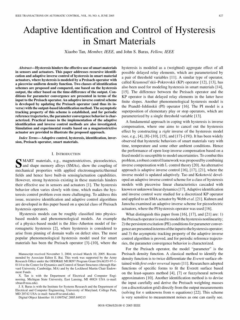
Theorem 3.2 is not conservative, and it covers a wide class ofPE inputs. For example, it can be easily verified that a (periodic)first order reversal input (see Fig. 4(a) for case ), whichhas been widely used for identification of Preisach density func-tion [11], and a (periodic) oscillating input with decreasing am-plitude (Fig. 4(b) for case ) both satisfy the conditionsin Theorem 3.2, and are thus PE. In these two cases, itselfsatisfies the conditions imposed for in the theorem. Fig. 5shows an example where one can conclude the PE of a periodic

by inspecting a PE equivalent input . Note that The-orem 3.2 does not require to be periodic, although periodicexamples are chosen here for easy illustration.

The PE conditions (Theorems 3.1 and 3.2) can be extendedwith some modifications to the case of identifying a piecewiseuniform density function. In the latter case, the input maytake any value in and is not restricted to the finiteset . Another difference is that the triangular shape ofdiagonal cells now helps in isolating contributions from thesecells (see the simulation results in Fig. 12 and the explanationin Section IV-B).

To be specific, one can show that a necessary condition forPE is that: There exists and an integer , such thatfor each , for any , one can find betweenand , with ; furthermore,for , there are at least input reversals in the block


Fig. 4. Examples of PE inputs (L = 4, showing one period). (a) First-orderreversal input. (b) Oscillating input with decaying amplitude.

Fig. 5. Example of PE input (L = 4, showing one period). The input u [n],PE equivalent to u[n], is obtained by swapping two sectionsA�B andA �Bof u[n].

with each local minimum andeach local maximum for some , . The proofwill be analogous to that of Theorem 3.1 except that one shouldfocus on isolation of contributions from inner cells instead ofdiagonal ones.

To adapt the sufficient condition Theorem 3.2, one changes“include all input levels ” to “visit all input bands,” “no morethan ” to “within neighboring input bands,” and requires eachlocal minimum and each local maximum

for some , . Here by input bands, we mean inputranges for . The proof will be nearlyidentical to that of Theorem 3.2.

C. Comparison of the Output-Based Scheme and theDifference-Based Scheme

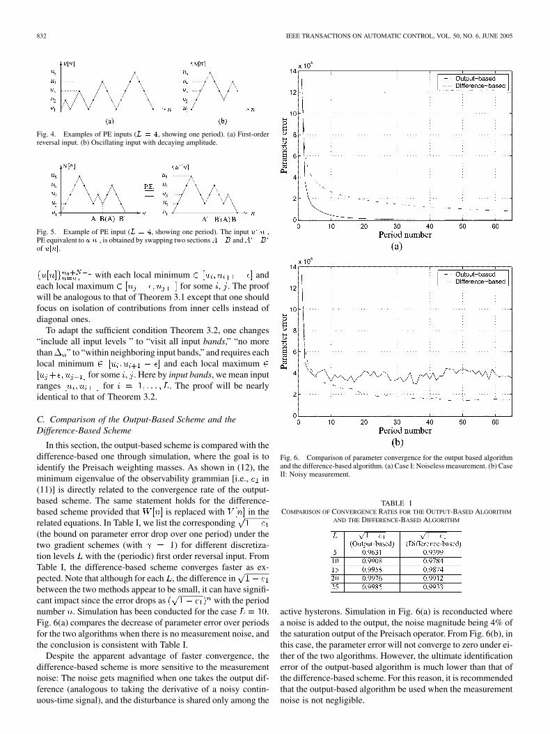
In this section, the output-based scheme is compared with thedifference-based one through simulation, where the goal is toidentify the Preisach weighting masses. As shown in (12), theminimum eigenvalue of the observability grammian [i.e., in(11)] is directly related to the convergence rate of the output-based scheme. The same statement holds for the difference-based scheme provided that is replaced with in therelated equations. In Table I, we list the corresponding(the bound on parameter error drop over one period) under thetwo gradient schemes (with ) for different discretiza-tion levels with the (periodic) first order reversal input. FromTable I, the difference-based scheme converges faster as ex-pected. Note that although for each , the difference inbetween the two methods appear to be small, it can have signifi-cant impact since the error drops as with the periodnumber . Simulation has been conducted for the case .Fig. 6(a) compares the decrease of parameter error over periodsfor the two algorithms when there is no measurement noise, andthe conclusion is consistent with Table I.

Despite the apparent advantage of faster convergence, thedifference-based scheme is more sensitive to the measurementnoise: The noise gets magnified when one takes the output dif-ference (analogous to taking the derivative of a noisy contin-uous-time signal), and the disturbance is shared only among the

Fig. 6. Comparison of parameter convergence for the output based algorithmand the difference-based algorithm. (a) Case I: Noiseless measurement. (b) CaseII: Noisy measurement.

TABLE ICOMPARISON OF CONVERGENCE RATES FOR THE OUTPUT-BASED ALGORITHM

AND THE DIFFERENCE-BASED ALGORITHM

active hysterons. Simulation in Fig. 6(a) is reconducted wherea noise is added to the output, the noise magnitude being 4% ofthe saturation output of the Preisach operator. From Fig. 6(b), inthis case, the parameter error will not converge to zero under ei-ther of the two algorithms. However, the ultimate identificationerror of the output-based algorithm is much lower than that ofthe difference-based scheme. For this reason, it is recommendedthat the output-based algorithm be used when the measurementnoise is not negligible.


Fig. 7. Preisach density function identified for different levels of discretizationL. (a) L = 5. (b) L = 10. (c) L = 15. (d) L = 25.

D. Experimental Results Based on a Magnetostrictive Actuator

Experiments have been conducted on a magnetostrictive (Ter-fenol-D) actuator to examine the identification schemes. Referto [20] for a description of the experimental setup. The displace-ment output of the actuator is controlled by the magnetic field

Fig. 8. CPU time used in the recursive gradient algorithm and the offlineleast-squares algorithm.

generated through the current in a coil. When operated in alow frequency range (typically below 5 Hz), the displacement

can be related to the bulk magnetization by a square lawfor some constant , and the current can

be related to the magnetic field along the rod direction by, where is the coil factor [30]. Then, the magne-

tostrictive hysteresis between and is fully captured by theferromagnetic hysteresis between and , which is modeledby the Preisach operator.

In the experiment a periodic first-order reversal input (withsufficiently dense distribution of turning points) is applied. Thechoice of the discretization level is of practical importance.Fig. 7 shows the identified density distribution for different dis-cretization levels after eight periods. The output-based gradientalgorithm is used with .

Although it is expected that the higher discretization level ,the higher model accuracy, there are two factors supporting amoderate value of in practice: The computational complexityand the sensor accuracy level. Since the number of cells on adiscretization grid scales as , so is the computational com-plexity of the recursive identification algorithm. It should alsobe noted that, from Table I, the convergence rate de-creases as increases. Fig. 8 shows the CPU time used in re-cursive identification for different discretization levels. To ob-tain the CPU time, the recursive algorithm is carried out againusing the collected data (the current and the displacement )of eight periods on a Dell laptop Inspiron 4150. Also, shown inFig. 8 is the CPU time it takes to compute the Preisach densityfunction using an offline, constrained least squares algorithm[8], where the data of one period were used. From Fig. 8, thesquare law for the recursive algorithm is evident. The offline al-gorithm becomes prohibitively time-consuming as gets large,due to the increasing complexity of solving a constrained opti-mization problem of many variables.

In the presence of the sensor noise and unmodeled dynamics,higher discretization level may not necessarily lead to improvedperformance. Fig. 9 compares the measured hysteresis loopsagainst the predicted loops based on the identified parametersfor different . Although the scheme with achieves


Fig. 9. Comparison of measured hysteresis loops with predicted loops basedon the identified Preisach density function. (a) L = 5. (b)L = 10. (c)L = 15.

much better match than the scheme with , there is little im-provement when is increased to 15. Hence for the Terfenol-Dactuator (and theLVDTsensorused), it isdetermined thatis an appropriate discretization level for the Preisach operator.

Fig. 10. Schematic of adaptive inverse control.

IV. ADAPTIVE INVERSE CONTROL

A. Adaptive Inverse Control Scheme

Fig. 10 shows a schematic of adaptive inverse control, whererepresents a Preisach operator with a piecewise uniform den-

sity function, and represents the Preisach operator with thecurrent density estimate. The input to is obtained through in-version of . The error between the reference trajectoryand the achieved trajectory is then used to update the pa-rameter estimate and thus the inverse model , wherethe output-based identification scheme (5) is used. Later on weshall also discuss the performance of adaptive inverse compen-sation using the difference-based parameter update (8), whichtypically fails to achieve asymptotic tracking.

The inversion scheme for is now briefly discussed. Letbe the memory curve of (and of ) at time ,

and be the saturation output corresponding to . Theinput to is generated through the following inversion al-gorithm.

A. If , ;B. If , ;C. Otherwise , where

is the (right) inverse of con-structed as in [20].

Let be the predicted output of . When, there exists no such that. Item A (item B, respectively) makes sure that

equals ( , respectively) and, hence, is closest to. On the other hand, when , can

be inverted exactly [20] and, therefore, .Theorem 4.1: Assume that the true Preisach operator has a

piecewise uniform density function. Denote by the -dimen-sional vector of true densities, and by the saturation outputcorresponding to . Let the output-based gradient algorithm beused for the parameter update. Then, the following hold.

1) For any reference trajectory with, the parameter estimate

for some , and the tracking erroras .

2) Assume that the density of the cell is pos-itive. Let be periodic of period that visits

, and without loss of generality .Define with thememory curve corresponding to the negative satura-tion, where is as constructed in [20]. Then,is also periodic with period , and . Letthe vector of signed areas of cells corresponding to

be (which is also periodic), and the null


space of be . Then, the param-eter estimate .In particular, if spans , .Analogous results hold if and visits

.Proof:

1) Define , and . Fromthe output-based gradient algorithm (lettingwithout loss of generality)

(13)

Since , as .This immediately results infor some . Summing (13) over leads to

, which implies. Since for some constant ,

as (14)

The Preisach operator based on can be exactlyinverted (hence ) except for the fol-lowing two cases: a) , andb) , where denotesthe saturation output corresponding to . For casea), the input under the inversion algorithm is

with , , and hence. The same conclusion

holds for the case b). It then follows from (14) that thetracking error approaches 0 as .

2) Since for each and, and the state of the Preisach

operator is reset at time . The periodicity ofthen follows from that of and the inverse

algorithm. From the first part of the theorem,and hence as .

Again, from , the input approachesas , and for

. As a consequence, .Since as

for

we conclude ,, i.e., . When spans

, and hence . Analogousarguments can be used for the case whereand visits .

Remark 4.1: Note that for the Preisach operator to have aunique (right) inverse, it is in general required that all diagonalcells have strictly positive density values [13]. However, whena particular inversion algorithm (e.g., the one in [20]) is used,the inverse trajectory can be made unique even if some diag-onal density values are zero. Therefore, in the statement ofTheorem 4.1 is well defined.

What happens if the difference-based algorithm (8) is used forparameter update in Fig. 10? Following the similar arguments asin the proof of Theorem 4.1, one can show for some

, and , where and are as definedin (6) and (7), respectively. This implies

(15)

From , . Even with a strong as-sumption as , one can only con-clude for some constant . Therefore,one cannot expect to achieve asymptotic tracking if the differ-ence-based scheme is adopted.

B. Simulation and Experimental Results

Simulation and experiments have been conducted to illustrateTheorem 4.1. Fig. 11(a) shows the simulation results of trackinga sinusoidal signal with amplitude using the output-basedadaptive inverse scheme. One can see that the tracking errorgoes to zero. Fig. 11(b) shows the simulation results of trackingwhere density parameters experience random changes of up to20% of their original values at , and the adaptive schemeis seen to suppress the tracking error quickly.

The simulation in Fig. 11(a) is continued for 160 periods, andFig. 12 compares the parameter estimates with the true param-eter values at the end of simulation. Note that the individualdensity values do not converge [Fig. 12(a)]. For this particularreference trajectory, the asymptotic input will be periodicvarying between and without other reversals. Hence,when is increasing, for each fixed , the components ofcorresponding to cells are equal; whenis decreasing, for each fixed , the components of corre-sponding to cells are equal. What separatesa diagonal cell from other cells of the row (or the column) is itstriangular shape. As a result, one expect that the densities of di-agonal cells will be correctly identified, and the sum of densitiesof cells in each row (or column) excluding the diagonal elementwill also be correctly identified. This is verified in Fig. 12(b),where by “aggregate cell density values,” we mean the quanti-ties , , and with , .

To further verify Part 2 of Theorem 4.1, simulation is alsoconducted for tracking an oscillating signal with decaying am-plitude for 128 periods (Fig. 13). The corresponding input to thedesired signal is PE, and indeed Fig. 14 shows the convergenceof individual cell density values.

Experimental results for tracking a sinusoidal signal areshown in Fig. 15 with two different adaptation constants . Inthese experiments and other experiments reported hereafter, thediscretization level . The current input applied to themagnetostrictive actuator is also displayed in addition to thereference trajectory, the achieved trajectory, and the trackingerror. It can be seen that when is smaller, the trajectory con-verges to the steady state slower but with smaller tracking errordue to lower sensitivity to the noise. Fig. 16 plots the achieveddisplacement versus the desired one at the steady-state (after 10s) for . The plot would overlap well with the 45 lineexcept for a small segment in the region , wherethe error is about . Considering the sensor precision,almost perfect tracking is achieved for the full operational


Fig. 11. (a) Simulation results of tracking a sinusoidal signal with amplitudey (L = 10). (b) Simulation results of tracking a sinusoidal signal withsudden parameter change at t = 5 s. (L = 10).

range (60 ) of the actuator. Note that error wasalso achieved by Natale et al. [10], however, there the trackingrange was 25 —about half of the range reported here.

If the reference trajectory does not cover , Theorem 4.1says that the tracking error still goes to zero, but one cannot saymore about the parameter convergence. In this case, there is noreset mechanisms during the adaptation, and depending on theinitial conditions of the system and the adaptation process, thefinal steady-state input trajectories can be different (while theoutput trajectories are all consistent with the reference trajec-tory). Essentially, there may exist multiple minor loops that sat-isfy the output requirement. To confirm this, two experiments

Fig. 12. Comparison of identified parameter values with true values aftertracking a sinusoidal signal for 160 periods (L = 10) for (a) individual celldensity values and (b) aggregate cell density values.

are conducted to track a sinusoidal trajectory of amplitude 15(and a dc offset of 30 ), one starting from the nega-

tive saturation and the other from the positive saturation. Thesteady-state current inputs obtained through adaptive inversecontrol are different, yet they are both able to track the desiredtrajectory. Fig. 17 plots the achieved displacement versus thecurrent for the two cases, and one can see that the ranges of cur-rent input differ by about 5%, but the displacement ranges areconsistent.

Finally, an experiment is performed to verify the analysis atthe end of Section IV-A. Here, the difference-based scheme (8)is used to update the density estimate during adaptation. Fig. 18shows the comparison of the desired trajectory and the achievedone, which clearly indicates that this scheme cannot achieveasymptotic tracking.

V. CONCLUSION AND DISCUSSIONS

This paper has been focused on recursive identification andadaptive inverse control of hysteresis in smart materials. A


Fig. 13. Simulation results of tracking an oscillating signal with decayingamplitude (L = 10, showing the first period).

Fig. 14. Comparison of identified density values of individual cells with truevalues after tracking an oscillating signal with decaying amplitude for 128periods (L = 10).

Preisach operator with piecewise uniform density function wasused to approximate smart material hysteresis. To facilitateanalysis and presentation, a Preisach operator with discreteweighting masses was also treated. A necessary conditionand a sufficient condition for the parameter convergence werepresented in terms of the hysteresis input. In contrast to theresults for linear systems, the conditions here are centeredaround the local maxima/minima (hence, reversals) of theinput. Asymptotic tracking under the output-based algorithmwas established, and the behavior of parameter convergencewas discussed for periodic reference trajectories. Although uni-form discretization of the Preisach plane was considered, theresults are applicable to the case of nonuniform discretization,as one can easily verify. Nonuniform discretization could be

Fig. 15. Experimental results of tracking a sinusoidal reference trajectory. (a) = 0:5. (b) = 0:2.

useful when the actual density function varies a lot in certainregion while changes little elsewhere.

Two types of adaptive gradient identification algorithmswere compared. Although the difference-based scheme cannotbe used for adaptive tracking, it can be a viable choice forrecursive parameter identification when the measurement noise


Fig. 16. Achieved displacement versus desired displacement (over the fulloperational range of the actuator) after 10 sec. of adaptation.

Fig. 17. Two minor loops corresponding to tracking a sinusoidal signal withamplitude less than y (at steady state).

is low. The introduction of a difference-based algorithm alsohelped in analyzing the PE conditions.

Computational complexity is one of the primary concernswhen it comes to real-time implementation. The inversion algo-rithm used in this paper was specifically developed for Preisachoperators with piecewise uniform densities. For each desiredoutput value, the algorithm finds its (exact) inverse in a finitenumber of iterations and thus is very efficient [20]. The level

of discretization determines the computational cost in bothinversion and adaptation. should be chosen based on avail-able computational resources, the sensor noise level, and thecontrol requirement. In particular, for our experimental setup,

Fig. 18. Experimental result showing that the difference-based adaptivescheme cannot achieve asymptotic tracking.

with the adaptive inversion scheme was able to virtu-ally cancel out the hysteresis effect in the actuator.

The asymptotic tracking result was based on the assumptionof time-invariant models. However, simulation indicated that theproposed scheme could adapt quickly should model parameterschange. It is expected that the scheme will work well in practiceas long as the hysteresis behavior changes at a relatively slowtime scale.

For future work, it will be of interest to extend the resultsreported here to the cases where the hysteresis output is notdirectly measurable. Such cases happen if, e.g., the high-fre-quency dynamics of the smart material actuator is not negligibleand hence a rate-independent hysteresis operator alone is inade-quate to capture the dynamic and hysteretic behavior [20], [31],or the actuator is used to control some other plant.

ACKNOWLEDGMENT

The authors wish to thank the anonymous reviewers for theirconstructive comments that helped in improving the paper.

REFERENCES

[1] S. O. R. Moheimani and G. C. Goodwin, “Guest editorial introductionto the special issue on dynamics and control of smart structures,” IEEETrans. Control Syst. Technol., vol. 9, pp. 3–4, 2001.

[2] D. C. Jiles and D. L. Atherton, “Theory of ferromagnetic hysteresis,” J.Magnet. Magn. Mater., vol. 61, pp. 48–60, 1986.

[3] A. A. Adly, I. D. Mayergoyz, and A. Bergqvist, “Preisach modelingof magnetostrictive hysteresis,” J. Appl. Phys., vol. 69, no. 8, pp.5777–5779, 1991.

[4] D. Hughes and J. T. Wen, “Preisach modeling and compensation forsmart material hysteresis,” in Active Materials and Smart Structures, ser.SPIE, G. L. Anderson and D. C. Lagoudas, Eds., 1994, vol. 2427, pp.50–64.

[5] J. Schäfer and H. Janocha, “Compensation of hysteresis in solid-stateactuators,” Sensors Actuators A, vol. 49, no. 1–2, pp. 97–102, 1995.

[6] P. Ge and M. Jouaneh, “Tracking control of a piezoceramic actuator,”IEEE Trans. Control Syst. Technol., vol. 4, pp. 209–216, 1996.

[7] R. B. Gorbet, D. W. L. Wang, and K. A. Morris, “Preisach model identi-fication of a two-wire SMA actuator,” in Proc. IEEE Int. Conf. Roboticsand Automation, 1998, pp. 2161–2167.


[8] X. Tan, R. Venkataraman, and P. S. Krishnaprasad, “Control ofhysteresis: Theory and experimental results,” in Modeling, SignalProcessing, and Control in Smart Structures, ser. SPIE, V. S. Rao, Ed.,2001, vol. 4326, pp. 101–112.

[9] D. Croft, G. Shed, and S. Devasia, “Creep, hysteresis, and vibration com-pensation for piezoactuators: Atomic force microscopy application,” J.Dyna. Syst., Measure., Control, vol. 123, no. 1, pp. 35–43, 2001.

[10] C. Natale, F. Velardi, and C. Visone, “Identification and compensationof Preisach hysteresis models for magnetostrictive actuators,” PhysicaB, vol. 306, pp. 161–165, 2001.

[11] I. D. Mayergoyz, Mathematical Models of Hysteresis. New York:Springer-Verlag, 1991.

[12] M. A. Krasnosel’skii and A. V. Pokrovskii, Systems With Hys-teresis. New York: Springer-Verlag, 1989.

[13] A. Visintin, Differential Models of Hysteresis. New York: Springer-Verlag, 1994.

[14] H. T. Banks, A. J. Kurdila, and G. Webb, “Identification of hystereticcontrol influence operators representing smart actuators, part I: Formu-lation,” Math. Prob. Eng., vol. 3, no. 4, pp. 287–328, 1997.

[15] W. S. Galinaitis and R. C. Rogers, “Control of a hysteretic actuator usinginverse hysteresis compensation,” in Mathematics and Control in SmartStructures, ser. SPIE, V. Varadan, Ed., 1998, vol. 3323, pp. 267–277.

[16] K. Kuhnen and H. Janocha, “Adaptive inverse control of piezoelectricactuators with hysteresis operators,” in Proc. European Control Conf.(ECC), Karsruhe, Germany, 1999, paper F 0291.

[17] G. Tao and P. V. Kokotovic, “Adaptive control of plants with unknownhysteresis,” IEEE Trans. Autom. Control, vol. 40, pp. 200–212, 1995.

[18] R. C. Smith, “Inverse compensation for hysteresis in magnetostrictivetransducers,” CRSC, North Carolina State Univ., Raleigh, NC, Tech.Rep. CRSC-TR98-36, 1998.

[19] L. Sun, C. Ru, W. Rong, L. Chen, and M. Kong, “Tracking controlof piezoelectric actuator based on a new mathematical model,” J. Mi-cromech. Microeng., vol. 14, pp. 1439–1444, 2004.

[20] X. Tan and J. S. Baras, “Modeling and control of hysteresis in magne-tostrictive actuators,” Automatica, vol. 40, no. 9, pp. 1469–1480, 2004.

[21] G. V. Webb, D. C. Lagoudas, and A. J. Kurdila, “Hysteresis modelingof SMA actuators for control applications,” J. Intell. Mater. Syst. Struct.,vol. 9, no. 6, pp. 432–448, 1998.

[22] K.-H. Hoffmann, J. Sprekels, and A. Visintin, “Identification of hys-teretic loops,” J. Comput. Phys., vol. 78, pp. 215–230, 1988.

[23] R. V. Iyer and M. E. Shirley, “Hysteresis parameter identification withlimited experimental data,” IEEE Trans. Magn., vol. 40, pp. 3227–3239,2004.

[24] X. Tan and J. S. Baras, “Recursive identification of hysteresis in smartmaterials,” in Proc. Amer. Control Conf., Boston, MA, 2004, pp.3857–3862.

[25] , “Adaptive inverse control of hysteresis in smart materials,” inProc. IFAC Symp. Nonlinear Control Systems, Stuttgart, Germany,2004.

[26] M. Brokate and J. Sprekels, Hysteresis and Phase Transitions. NewYork: Springer-Verlag, 1996.

[27] X. Tan, “Control of smart actuators,” Ph.D. dissertation, Univ. Maryland,College Park, MD, 2002.

[28] G. C. Goodwin and K. S. Sin, Adaptive Filtering, Prediction and Con-trol. Upper Saddle River, NJ: Prentice-Hall, 1984.

[29] S. Sastry and M. Bodson, Adaptive Control: Stability, Convergence, andRobustness. Upper Saddle River, NJ: Prentice-Hall, 1989.

[30] R. Venkataraman, “Modeling and adaptive control of magnetostrictiveactuators,” Ph.D. dissertation, Univ. Maryland, College Park, MD, 1999.

[31] D. Davino, C. Natale, S. Pirozzi, and C. Visone, “Phenomenologicaldynamic model of a magnetostrictive actuator,” Physica B, vol. 343, pp.112–116, 2004.

Xiaobo Tan (S’97–M’02) was born in Danyang,China, in 1972. He received the B.S. and M.S. de-grees in automatic control from Tsinghua University,Beijing, China, in 1995 and 1998, respectively, andthe Ph.D. degree in electrical and computer engi-neering from the University of Maryland, CollegePark, in 2002. His Ph.D. dissertation was focusedon modeling and control of hysteresis in smartactuators.

From September 2002 to July 2004, he was a Re-search Associate with the Institute for Systems Re-

search (ISR), the University of Maryland. In August 2004, he joined the De-partment of Electrical and Computer Engineering, Michigan State University,East Lansing, as an Assistant Professor. His research interests include modelingand control of smart materials and micro-electromechanical systems, distributedcontrol of networked systems, and numerical integration of dynamical systemson manifolds.

Dr. Tan was an ISR Systems Fellow from 1998 to 2002. He was a finalist forthe Best Student Paper Award at the 2002 IEEE Conference on Decision andControl, and a co-recipient of the Best Poster Award at the Greater Washington-Baltimore Area MEMS Alliance Special Topics Symposium in April 2003.

John S. Baras (S’73–M’73–SM’83–F’84) receivedthe B.S. degree in electrical engineering from theNational Technical University of Athens, Athens,Greece, in 1970, and the M.S. and Ph.D. degreesin applied mathematics from Harvard University,Cambridge, MA, in 1971 and 1973, respectively.

Since 1973, he has been with the Electrical andComputer Engineering Department and the AppliedMathematics Faculty, the University of Maryland,College Park, where he is currently a Professor andthe Lockheed Martin Chair in Systems Engineering.

He was the Founding Director of the Institute for Systems Research (ISR,one of the first six NSF ERCs) from 1985 to 1991, and has been the Directorof the Center for Hybrid and Satellite Communication Networks (a NASACenter for the Commercial Development of Space) since 1991. His researchinterests include integration of logic programming and nonlinear programmingfor tradeoff analysis, object-oriented modeling, validation, and verification ofcomplex systems models and engineering designs, hybrid, satellite and wirelesscommunication networks, integrated network management systems, networksecurity, stochastic systems, robust control of nonlinear systems, real-time par-allel architectures for nonlinear signal processing, intelligent control systems,expert and symbolic systems for control and communication systems synthesis,biomimetic algorithms and systems for signal processing and sensor networks,and intelligent manufacturing of smart materials. He has published over 350technical articles on control, communication and computing systems, and wasthe Editor of the book Recent Advances in Stochastic Calculus (New York:Springer-Verlag, 1990).

Dr. Baras has served on the Board of Governors of the IEEE Control SystemsSociety, IEEE Engineering R&D Committee, Aerospace Industries AssociationAdvisory Committee on Advanced Sensors, and the IEEE Fellow evaluationcommittee. He is currently serving on the Editorial Boards of Mathematics ofControl, Signals, and Systems, of Systems and Control: Foundations and Appli-cations, the IMA Journal of Mathematical Control and Information, and SystemsAutomation-Research and Applications. He has received the 1978, 1983, and1993 Naval Research Laboratory Research (Alan Berman) Publication Awards,the 1980 Outstanding Paper Award of the IEEE Control Systems Society, the1996 Outstanding Paper Award at Design SuperCon, and the 2002 Best PaperAward at the 23rd Army Science Conference.

ieee transactions on automatic control, … · oped an adaptive inverse control scheme for a class...

Documents