identifying the factors responsible for loan defaults and ...the loan data for december 2015 was...
TRANSCRIPT

1
MWSUG 2016 - Paper AA02
Identifying the factors responsible for loan defaults and classification of customers using SAS® Enterprise Miner
Juhi Bhargava, Oklahoma State University, Stillwater, OK Prashanth Reddy Musuku, Oklahoma State University, Stillwater, OK
ABSTRACT
Lending business is crucial to the profitability of a bank or financial institution. Loan defaults, delay in repayment by customers lead to problems in cash flow position. The last economic crisis in US was triggered by loan defaults.
This study aims to identify the factors contributing towards loan defaults, delay in repayments as well as the characteristics of a borrower who will honor all the obligations of a loan. The results enable us to determine the relationship between loan and customer characteristics and the probability to default. The results may also be used to appraise and monitor credit risk at the time of loan approval and during the currency of the loan.
The data set consists of all loans issued through December, 2015 along with the loan status. It contains 111 variables such as the details of customer’s loan account, amount, application type – individual or joint, principal outstanding, amount paid, interest rate, length of employment, annual income, loan status, verification status, purpose of loan and so on. Loan status has several levels – current, default, in grace or late due. There were 421,095 records in the dataset.
The factors contributing towards loan default were identified and predicted using models such as logistic regression, decision tree and artificial neural networks. The identified factors will then be implemented using random forest method to classify the customers whether they are good loans or bad loans. The classification will enable the lending institutions and investors to optimize their policies and strategies to reduce the loan defaults and also to make informed decisions about the current customers at the risk of default.
INTRODUCTION
The loan data for December 2015 was extracted from the website of Lending Club, an online credit market place. Lending Club facilitates the borrowing and lending of loans. All its operations are online and has no branch infrastructure, unlike banks. Personal loans, business loans and medical finance form the portfolio of Lending Club. To date, Lending Club has facilitated over 20 billion dollars in loans with an annual net return rate of 7.55%. In light of these high returns and the increasing popularity, it is imperative to understand the characteristics which make a loan good or lead to default.
DATA COLLECTION AND PREPARATION
The data was downloaded from the Lending Club website, an online market place. The final dataset contained the following variables.
Role Level Count
ID Nominal 1
Input Interval 79
Input Nominal 15
Target Nominal 1
Figure 1. Variable Summary
2
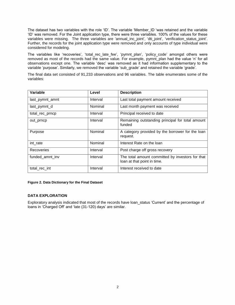
The dataset has two variables with the role ‘ID’. The variable ‘Member_ID ‘was retained and the variable ‘ID’ was removed. For the Joint application type, there were three variables. 100% of the values for these variables were missing. The three variables are ‘annual_inc_joint’, ‘dti_joint’, ‘verification_status_joint’. Further, the records for the joint application type were removed and only accounts of type individual were considered for modeling.
The variables like ‘recoveries’, ‘total_rec_late_fee’, ‘pymnt_plan’, ‘policy_code’ amongst others were removed as most of the records had the same value. For example, pymnt_plan had the value ‘n’ for all observations except one. The variable ‘desc’ was removed as it had information supplementary to the variable ’purpose’. Similarly, we removed the variable ‘sub_grade’ and retained the variable ‘grade’.
The final data set consisted of 91,233 observations and 96 variables. The table enumerates some of the variables:
Variable Level Description
last_pymnt_amnt Interval Last total payment amount received
last_pymnt_d Nominal Last month payment was received
total_rec_prncp Interval Principal received to date
out_prncp Interval Remaining outstanding principal for total amount funded
Purpose Nominal A category provided by the borrower for the loan request.
int_rate Nominal Interest Rate on the loan
Recoveries Interval Post charge off gross recovery
funded_amnt_inv Interval The total amount committed by investors for that loan at that point in time.
total_rec_int Interval Interest received to date
Figure 2. Data Dictionary for the Final Dataset
DATA EXPLORATION
Exploratory analysis indicated that most of the records have loan_status ‘Current’ and the percentage of loans in ‘Charged Off’ and ‘late (31-120) days’ are similar.

3
Figure 3. Distribution of Target Variable Loan_Status
From the dataset, observations with loan status ‘Current’ were not considered for modeling as these are considered loans which are still making payments within timelines. The observations in the final dataset belonged to one of the six types of loan_status. The variable was converted into a binary variable with the levels ‘1’ and ‘0’. Level ‘1’ included ‘Charged Off’, ‘Default’ and ‘Late (31 – 120days)’. Level ‘0’ included ‘Fully Paid’, ‘In Grace period’ and ‘late (16 – 30 days)’. This conversion done by Replacement node. Imputation of variables with missing values done using Tree method for class variables and using Median for the interval variables. ‘Max Normal’ method was used to transform variables.
DATA PARTITION
Data was partitioned into Training data (70%) and Validation data (30%) based on the optimal method of partition ratio, which was required for modeling.
VARIABLE CLUSTERING AND SELECTION
The high number of variables in the dataset causes problems of collinearity and redundancy. Variable clustering node helped in choosing the optimum number of variables. Criterion for variable clustering was correlation. We have elected the representative variable for the cluster using the value for 1-R-square.The variable clustering node created 20 clusters.
Variable Selection node selects the important input variables based on the statistic R-square to predict the target variables. This node rejected variables with low R-square. For this paper, variables with R-square above 0.005 taken as the selection criterion.

4
Figure 4. Variables selected through variable clustering
MODELING
1. Decision Tree
Decision tree was the initial model, as our target was a binary target and the tree will enable us to build a strategy to identify loan defaults by making classifications and setting up rules and also to understand the interrelation between the variables by studying each node of classification of the decision tree.
The important variables from Decision Tree are in Output 1. Decision tree considered variables like term, last_pymnt_d for decision-making.
Output 1. Important variables from Decision Tree
Output 2. Sensitivity Analysis

5
There were a total 21 leaf nodes in the tree diagram.
The English rules for a loan to turn out as a bad loan is
WHERE Transformed: Replacement: total_rec_prncp < 0.581 AND
Transformed: Imputed last_pymnt_d _OTHER_ Or Missing AND
Transformed: Replacement: total_rec_prncp < 0.4889 Or Missing AND
Transformed: Replacement: total_rec_prncp < 0.4108
In case for a loan to turn out as a good loan,
WHERE Transformed: Replacement: total_rec_prncp >= 0.581 Or Missing AND
Transformed: Replacement: out_prncp_inv < 0.0082 Or Missing AND
Transformed: Replacement: collection_recovery_fee < 0.0608 Or Missing AND
Transformed: Replacement: total_rec_prncp >= 0.6147 Or Missing AND
Transformed: Replacement: total_rec_prncp >= 0.6913 Or Missing
Output 3. Decision Tree
2. Logistic Regression
Logistic regression model provides prediction for the binary target variable ‘loan_status’ by estimating probabilities, that help in predicting the results for the new cases, with a comparatively higher degree of accuracy.
Stepwise regression was the chosen variable selection method. This method chose ten variables, some of them being transformed variables. Variables chosen are – PWR_REP_total_rec_prncp, SQRT_REP_collection_recovery_fee, SQRT_REP_out_prncp_inv, and TG_IMP_last_pymnt_d.

6
Output 4. Output from Logistic Regression Model
Output 5. Sensitivity Analysis

7
Output 6. Effects Plot
The Effects Plot provides whether predictors have a positive effect or a negative effect on the response variable new_tar. From the Effects Plot,
SQRT_REP_collection_recovery_fee has a positive effect with an absolute coefficient of 66.75638
PWR_REP_total_rec_prncp has a negative effect with an absolute coefficient of 17.19229
Intercept has a positive effect with an absolute coefficient of 6.907717
SQRT_REP_out_prncp_inv has a positive effect with an absolute coefficient of 2.833697
TG_IMP_last_pymnt_dJUL_16 has a negative effect with an absolute coefficient of 1.858424
Similar to the decision tree, total principal received, last payment date, collection recovery fee and outstanding principal play a role in deciding whether a loan will be good or bad.
3. Neural Networks
Neural network models provide an algorithm to determine the effects of interactions of various variables on the target variable. This model is useful to solve business problems with a lot of data and several variables.
From the iteration plot for misclassification rate, an optimized solution was obtained aftrer 11 iterations.
Output 7. Parameter Estimates from Neural Networks Model

8
Output 8. Sensitivity Analysis
4. Random Forest
Random forest is an ensemble model and can be effectively used for classification. This model constructs several decision trees on the training data. The model then combines trees having low correlation. This model deals well with imbalanced data.
Output 9. Classification Table from Random Forest Model

9
Output 10. Output from Random Forest Model
From the Leaf Statistics plot, we observed that there was a decline after 80.4 trees even though additional training was given.
Output 11. Output from Model

10
Output 12. Output from Model
MODEL COMPARISION
Comparing the validation Misclassification Rate for the models, HP Forest had the lowest misclassification rate and hence was chosen to be the best model as the target was binary.
Output 13. Output from Model

11
Output 14. Output from Model
Model Misclassification Rate
HP Forest 0.05619
Decision Tree 0.05966
Neural Network 0.07672
Logistic Regression 0.08016
Output 15. Output from Model
CONCLUSION
To identify the characteristics of a loan default, the loan status, which go into defining a good loan and a bad loan was converted into a binary target variable. Further, data preparation was done by exploring the variables for the type of values, the missing percentage and redundancy.
Models employed were decision tree, logistic regression, neural networks and random forest. These models were chosen to make classification of characteristics underlying a good loan and bad loan, and to make predictions thereon. These models also are good for large and imbalanced data sets. HP Forest was the best model as it had the lowest misclassification rate.
Intuitively, loan default cases are attributable to total principal received, outstanding principal, and last payment date. A higher principal would imply higher risk of default. The logistic regression model considered all these variables. Credit appraisal at the time of loan sanction takes into account the risk along with the capacity of the borrower to repay. Principal amount determines the periodic repayment amount. These characteristics will help in determining the loan defaults in future. Further, this also determines the loan term.

12
While these details govern loan quality, the intention of the borrower to repay is another important consideration. This is where verification status comes in. Regular and timely repayments characterize a good loan.
An ongoing review of these variables would help monitor loan status and risk of default by an investor.
Briefly, quantum of repayment amount, the regularity of payments, and loan grade contribute toward making a loan a good loan or a bad loan.
REFERENCES
Lending Club Statistics June 30, 2016 Available at https://www.lendingclub.com/info/statistics.action
Lending Club Statistics as of July 31, 2016 Available at https://www.lendingclub.com/info/demand-and-credit-profile.action
Renton, Peter Lending Club Review for New Investors Lend Academy June, 2015. Available at http://www.lendacademy.com/lending-club-review/
N. V. Chawla, N. Japkowicz, and A. Ko lcz, editors, Special Issue on Learning from Imbalanced Data Sets
Identifying Potential Default Loan Applicants - A Case Study of Consumer Credit Decision for Chinese Commercial Bank1. Gan , Qiwei, Luo , Binjie; Lin , Zhangxi , Proceedings of the SAS Global 2008 Conference Available at http://www2.sas.com/proceedings/forum2008/159-2008.pdf
SAS Enterprise Miner Example for Predictive Modeling Available at https://communities.sas.com/kntur85557/attachments/kntur85557/data_mining/538/1/PredictiveModeling.pdf
SAS Institute Inc. 2003. Data Mining Using SAS® Enterprise MinerTM: A Case Study Approach, Second Edition. Cary, NC: SAS Institute Inc. Available at https://support.sas.com/documentation/onlinedoc/miner/casestudy_59123.pdf
ACKNOWLEDGMENTS
We thank MWSUG for giving us an opportunity to present our work. We also thank Dr. Goutam Chakraborty and Dr. Miriam McGaugh for their guidance and support.
CONTACT INFORMATION
Your comments and questions are valued and encouraged. Contact the author at:
Name: Juhi Bhargava
Enterprise: Oklahoma State University
Address: Stillwater
City, State ZIP: OK, 74078
Work Phone: 405-780-5640
E-mail: [email protected]
Name: Prashanth Reddy Musuku
Enterprise: Oklahoma State University

13
Address: Stillwater
City, State ZIP: OK, 74078
Work Phone: 732-770-3399
E-mail: [email protected]
SAS and all other SAS Institute Inc. product or service names are registered trademarks or trademarks of SAS Institute Inc. in the USA and other countries. ® indicates USA registration.
Other brand and product names are trademarks of their respective companies.