identification of protein interaction partners and protein-protein interaction sites

doi:10.1016/j.jmb.2008.08.002 J. Mol. Biol. (2008) 382, 1276–1289

Available online at www.sciencedirect.com

Identification of Protein Interaction Partners andProtein–Protein Interaction Sites

Sophie Sacquin-Mora1⁎, Alessandra Carbone2,3 and Richard Lavery4

1Laboratoire de BiochimieThéorique, CNRS UPR 9080,Institut de BiologiePhysico-Chimique, 13 ruePierre et Marie Curie,75005 Paris, France2Département d'Informatique,Université Pierre et MarieCurie - Paris 6,UMRS511, 91 Blvde l'Hopital, 75013 Paris, France3Génomique Analytique,INSERM U511, 75013 Paris,France4Institut de Biologie et Chimie desProtéines, CNRS UMR 5086 /IFR 128 / Université de Lyon 7passage du Vercors, 69367 Lyon,France

Received 19 March 2008;received in revised form10 July 2008;accepted 1 August 2008Available online7 August 2008

*Corresponding author. E-mail addrAbbreviations used: CC-D, comp

PDB, Protein Data Bank.

0022-2836/$ - see front matter © 2008 E

Rigid-body docking has become quite successful in predicting the correctconformations of binary protein complexes, at least when the constituentproteins do not undergo large conformational changes upon binding.However, determining whether two given proteins interact is a moredifficult problem. Successful docking procedures often give equally goodscores for proteins that do not interact experimentally. This is the case for themultiple minimization approach we use here. An analysis of the resultswhere all proteins within a set are docked with all other proteins (completecross-docking) shows that the predictions can be greatly improved if thelocation of the correct binding interface on each protein is known, since theexperimental complexes are much more likely to bring these two interfacesinto contact, at the same time as yielding good interaction energy scores.While various methods exist for identifying binding interfaces, it is shownthat simply studying the interaction of all potential protein pairs within adata set can itself help to identify the correct interfaces.

© 2008 Elsevier Ltd. All rights reserved.

Edited by M. Sternberg
Keywords: protein–protein interactions; docking simulations; coarse-grained model; binding site; binding interface
Introduction

Protein–protein interactions are crucial in mostbiological processes, including metabolism, signal-ing, gene expression, and immune responses. More-over, the availability of complete genome sequencesand high-throughput analysis techniques havebroadened the focus from a single interaction tothe whole proteome, and have made the identifica-tion of functional protein complexes, and a betterunderstanding of how they form in the crowdedcellular environment, a major goal of biology.1–3

ess: [email protected] cross-docking;

lsevier Ltd. All rights reserve

Many experimental approaches, including yeasttwo-hybrid analysis, mass spectroscopy and affinitypurification,4–8 have been developed for the detec-tion and identification of interacting proteins in thecellular context, leading to a wealth of data and thedevelopment of protein interaction databases.9–11

Various bioinformatics approaches have also beenused to identify interactions including gene cluster-ing and phylogenetic profiling12 All these methods,however, have their drawbacks and can result inconsiderable numbers of false positives andnegatives.13 These methods also identify interac-tions without providing the structure of the corre-sponding complex, whereas this structure is often akey element in understanding function.Molecular modeling offers an alternative to these

approaches which, if successful, could help inidentifying relevant interactions, at the same time

d.

1277Protein Interaction Partners

as providing structural models of the correspondingcomplexes and clarifying the physical principlesbehind the complex formation.While protein–protein docking has become amajor

goal for biophysics and computational biology overthe last 30 years,14–20 docking algorithms havelargely been restricted to determining the conforma-tion of complexes between protein partners that areknown to interact. This problem is now being solvedmore and more successfully, especially when com-plex formation does not lead tomajor conformationalchanges in the interacting partners.17,21 However,almost no attention has been given to the problem ofusing docking to identify true interacting partners.Identifying interacting partnerswithin an arbitrary

set of proteins is clearly difficult. Here, we attack thisproblem via complete cross-docking (CC-D), whichinvolves performing docking calculations on all thepossible protein pairs within a given dataset and notonly on protein pairs that have already beenidentified experimentally as forming complexes,and therefore N2 docking trials for N proteins. Toour knowledge, this is the first time that suchcalculations have been carried out in a systematicway. Previous related studies have been limited tolooking at the interaction of a single protein(lysozyme) with three potential receptors (chymo-trypsin, cytochrome f andUDG),22 at the competitionof small ligands for a single enzymatic binding site(sometimes termed cross-docking),23–28 or at thedocking of various conformations of the receptor andligand proteins for a single complex.29–33

WehaveusedCC-Dwith a set of 12 proteins knownto form six binary complexes. We used a rigid-bodydocking algorithm combined with a coarse-grainprotein representation to test all potential interactionsand showed that while this approach predicts goodconformations for the experimentally known part-ners, it completely fails to identify these partnersamongst the numerous alternative interactions whenconsidering the protein interaction energy alone.However, adding accurate data on the location ofthe correct interface residues greatly improves thescoring function and allows the identification of theexperimental partner for each protein in the set. Weshow also that CC-D can itself provide information

Table 1. Summary of the protein complexes investigated in t

Complexa

(boundstructures)

PDB 1a

(unboundstructure)

PDB 2a

(unboundstructure)

1BRS(A:D) 1A2P(B) 1A19(A)2PTC(E:I) 2PTN 6PTI

1FSS(A:B) 2ACE(E) 1FSC

2TEC(E:I) 1THM 2TEC(I)1UGH(E:I) 1AKZ 1UGI(A)

1GRN(A:B) 1A4R(A) 1RGPa PDB55 code for the crystal structure used in this study with the cb Number of residues of the protein in parenthesis.

on the correct binding interfaces, and can conse-quently improve predictions.

Results

TheMAXDoprogram, (seeMaterials andMethods)has been applied to a test set of six binaryprotein com-plexes (see Table 1) comprising 12 distinct proteinswith sizes ranging from 50 to N 500 residues. Herefurther references to these proteins use their name orthe PDB code of the complex they belong to, plus thechain ID of the protein (Table 1). For example, 1BRS-A and 1BRS-D refer to barnase (A) and barstar (D) inthe barnase–barstar complex 1BRS. The coordinatesfor the bound and unbound conformations of bothreceptor and ligand proteins, are available in theProtein Data Bank, and they belong to the dockingbenchmarks that were developed by Chen et al.34 35

For this preliminary study we have chosen fivecomplexes that correspond to enzyme–inhibitorinteractions and one that is an enzyme–activatorcomplex. Each protein was docked on all the proteinsof the dataset (including itself). Since the receptor andthe ligand proteins have distinct roles in our dockingalgorithm, every pair of proteins A and Bwas studiedtwice, with first A and then B being treated as thereceptor. Except for 1GRN, all the complexes of ourdataset belong to the “rigid-body” category of thedocking benchmark.35 In 1GRN, complex formationleads to a 1.22 Å root-mean-square deviation (rmsd)change in the Cα atoms of the interface residues.Although the proteins we study generally undergoonly minor backbone conformational changes uponassociation, there can be many side chain reorienta-tions. We have consequently done two series of tests,interacting either the bound or the unbound con-formations, to evaluate the impact of these changes.

Simple docking and energy maps

In order to validate our docking algorithm,we firsttested it on the experimentally known complexes.For each complex, themethodwas able to predict theposition of the ligand protein correctly with respectto its receptor with an rmsd of the Cα pseudoatoms

his study

Protein 1b Protein 2b

Barnase (110) Barstar (89)β-Trypsin (245) Pancreatic trypsin

inhibitor (PTI) (57)Snake venom

acetylcholinesterase (535)Fasciculin II (61)

Thermitase (279) Eglin C (63)Human Uracil-DNAglycosylase (223)

Inhibitor (UDGI) (84)

CDC42 GTPase (200) CDC42 GAP (199)

hain IDs in parenthesis.

1278 Protein Interaction Partners

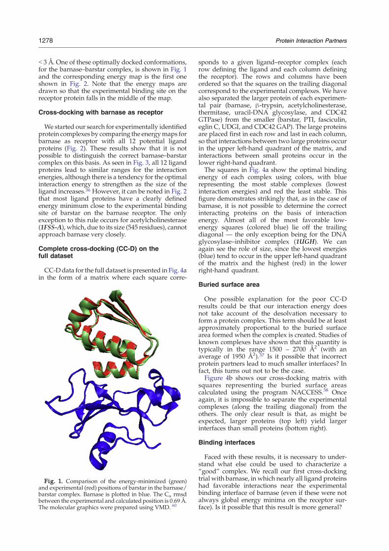
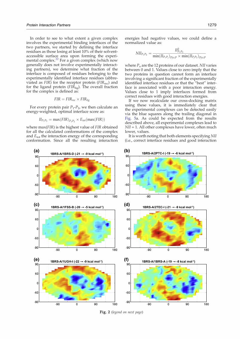
b 3 Å. One of these optimally docked conformations,for the barnase–barstar complex, is shown in Fig. 1and the corresponding energy map is the first oneshown in Fig. 2. Note that the energy maps aredrawn so that the experimental binding site on thereceptor protein falls in the middle of the map.

Cross-docking with barnase as receptor

We started our search for experimentally identifiedprotein complexes by comparing the energymaps forbarnase as receptor with all 12 potential ligandproteins (Fig. 2). These results show that it is notpossible to distinguish the correct barnase–barstarcomplex on this basis. As seen in Fig. 3, all 12 ligandproteins lead to similar ranges for the interactionenergies, although there is a tendency for the optimalinteraction energy to strengthen as the size of theligand increases.36 However, it can be noted in Fig. 2that most ligand proteins have a clearly definedenergy minimum close to the experimental bindingsite of barstar on the barnase receptor. The onlyexception to this rule occurs for acetylcholinesterase(1FSS-A), which, due to its size (545 residues), cannotapproach barnase very closely.

Complete cross-docking (CC-D) on thefull dataset

CC-Ddata for the full dataset is presented in Fig. 4ain the form of a matrix where each square corre-

Fig. 1. Comparison of the energy-minimized (green)and experimental (red) positions of barstar in the barnase/barstar complex. Barnase is plotted in blue. The Cα rmsdbetween the experimental and calculated position is 0.69 Å.The molecular graphics were prepared using VMD. 60

sponds to a given ligand–receptor complex (eachrow defining the ligand and each column definingthe receptor). The rows and columns have beenordered so that the squares on the trailing diagonalcorrespond to the experimental complexes. We havealso separated the larger protein of each experimen-tal pair (barnase, β-trypsin, acetylcholinesterase,thermitase, uracil-DNA glycosylase, and CDC42GTPase) from the smaller (barstar, PTI, fasciculin,eglin C, UDGI, and CDC42 GAP). The large proteinsare placed first in each row and last in each column,so that interactions between two large proteins occurin the upper left-hand quadrant of the matrix, andinteractions between small proteins occur in thelower right-hand quadrant.The squares in Fig. 4a show the optimal binding

energy of each complex using colors, with bluerepresenting the most stable complexes (lowestinteraction energies) and red the least stable. Thisfigure demonstrates strikingly that, as in the case ofbarnase, it is not possible to determine the correctinteracting proteins on the basis of interactionenergy. Almost all of the most favorable low-energy squares (colored blue) lie off the trailingdiagonal — the only exception being for the DNAglycosylase–inhibitor complex (1UGH). We canagain see the role of size, since the lowest energies(blue) tend to occur in the upper left-hand quadrantof the matrix and the highest (red) in the lowerright-hand quadrant.

Buried surface area

One possible explanation for the poor CC-Dresults could be that our interaction energy doesnot take account of the desolvation necessary toform a protein complex. This term should be at leastapproximately proportional to the buried surfacearea formed when the complex is created. Studies ofknown complexes have shown that this quantity istypically in the range 1500 – 2700 Å2 (with anaverage of 1950 Å2).37 Is it possible that incorrectprotein partners lead to much smaller interfaces? Infact, this turns out not to be the case.Figure 4b shows our cross-docking matrix with

squares representing the buried surface areascalculated using the program NACCESS.38 Onceagain, it is impossible to separate the experimentalcomplexes (along the trailing diagonal) from theothers. The only clear result is that, as might beexpected, larger proteins (top left) yield largerinterfaces than small proteins (bottom right).

Binding interfaces

Faced with these results, it is necessary to under-stand what else could be used to characterize a“good” complex. We recall our first cross-dockingtrial with barnase, in which nearly all ligand proteinshad favorable interactions near the experimentalbinding interface of barnase (even if these were notalways global energy minima on the receptor sur-face). Is it possible that this result is more general?


In order to see to what extent a given complexinvolves the experimental binding interfaces of thetwo partners, we started by defining the interfaceresidues as those losing at least 10% of their solvent-accessible surface area upon forming the experi-mental complex.22 For a given complex (which nowgenerally does not involve experimentally interact-ing partners), we determine what fraction of theinterface is composed of residues belonging to theexperimentally identified interface residues (abbre-viated as FIR) for the receptor protein (FIRrec) andfor the ligand protein (FIRlig). The overall fractionfor the complex is defined as:

FIR ¼ FIRrec � FIRlig

For every protein pair P1-P2, we then calculate anenergy-weighted, optimal interface score as:

IIP1P2 ¼ maxðFIRÞP1P2� EtotðmaxðFIRÞÞ

where max(FIR) is the highest value of FIR obtainedfor all the calculated conformations of the complexand Etot the interaction energy of the correspondingconformation. Since all the resulting interaction

Fig. 2 (legend o

energies had negative values, we could define anormalized value as:

NIIP1P2 ¼II2P1P2

minðIIP1PjÞPjaP �minðIIPjP2ÞPjaP

where Pn are the 12 proteins of our dataset.NII variesbetween 0 and 1. Values close to zero imply that thetwo proteins in question cannot form an interfaceinvolving a significant fraction of the experimentallyidentified interface residues or that the “best” inter-face is associated with a poor interaction energy.Values close to 1 imply interfaces formed fromcorrect residues with good interaction energies.If we now recalculate our cross-docking matrix

using these values, it is immediately clear thatthe experimental complexes can be detected easilyvia the blue squares along the trailing diagonal inFig. 5a. As could be expected from the resultsdescribed above, all experimental complexes lead toNII = 1. All other complexes have lower, often muchlower, values.It is worth noting that both elements specifyingNII

(i.e., correct interface residues and good interaction

n next page)

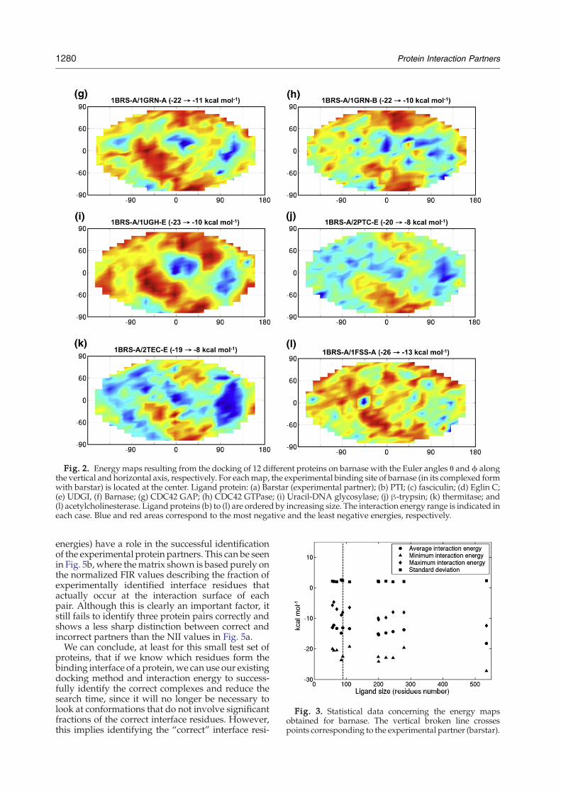
Fig. 2. Energy maps resulting from the docking of 12 different proteins on barnase with the Euler angles θ and ϕ alongthe vertical and horizontal axis, respectively. For eachmap, the experimental binding site of barnase (in its complexed formwith barstar) is located at the center. Ligand protein: (a) Barstar (experimental partner); (b) PTI; (c) fasciculin; (d) Eglin C;(e) UDGI, (f) Barnase; (g) CDC42 GAP; (h) CDC42 GTPase; (i) Uracil-DNA glycosylase; (j) β-trypsin; (k) thermitase; and(l) acetylcholinesterase. Ligand proteins (b) to (l) are ordered by increasing size. The interaction energy range is indicated ineach case. Blue and red areas correspond to the most negative and the least negative energies, respectively.

Fig. 3. Statistical data concerning the energy mapsobtained for barnase. The vertical broken line crossespoints corresponding to the experimental partner (barstar).


energies) have a role in the successful identificationof the experimental protein partners. This can be seenin Fig. 5b, where thematrix shown is based purely onthe normalized FIR values describing the fraction ofexperimentally identified interface residues thatactually occur at the interaction surface of eachpair. Although this is clearly an important factor, itstill fails to identify three protein pairs correctly andshows a less sharp distinction between correct andincorrect partners than the NII values in Fig. 5a.We can conclude, at least for this small test set of

proteins, that if we know which residues form thebinding interface of a protein, we can use our existingdocking method and interaction energy to success-fully identify the correct complexes and reduce thesearch time, since it will no longer be necessary tolook at conformations that do not involve significantfractions of the correct interface residues. However,this implies identifying the “correct” interface resi-

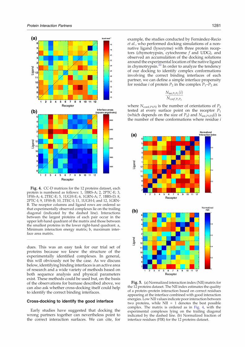
Fig. 4. CC-D matrices for the 12 proteins dataset, eachprotein is numbered as follows: 1, 1BRS-A; 2, 2PTC-E; 3,1FSS-A; 4, 2TEC-E; 5, 1UGH-E; 6, 1GRN-A; 7, 1BRS-D; 8,2PTC-I; 9, 1FSS-B; 10, 2TEC-I; 11, 1UGH-I; and 12, 1GRN-B. The receptor columns and ligand rows are ordered sothat experimentally observed complexes lie on the trailingdiagonal (indicated by the dashed line). Interactionsbetween the largest proteins of each pair occur in theupper left-hand quadrant of the matrix and those betweenthe smallest proteins in the lower right-hand quadrant. a,Minimum interaction energy matrix; b, maximum inter-face area matrix.

Fig. 5. (a)Normalized interaction index (NII)matrix forthe 12 proteins dataset. The NII index estimates the qualityof a protein–protein interaction based on correct residuesappearing at the interface combined with good interactionenergies. LowNII values indicate poor interaction betweentwo proteins, while NII = 1 denotes the best possiblecomplex. The matrix is ordered as in Fig. 4, with theexperimental complexes lying on the trailing diagonalindicated by the dashed line. (b) Normalized fraction ofinterface residues (FIR) for the 12 proteins dataset.


dues. This was an easy task for our trial set ofproteins because we knew the structure of theexperimentally identified complexes. In general,this will obviously not be the case. As we discussbelow, identifying binding interfaces is an active areaof research and a wide variety of methods based onboth sequence analysis and physical parametersexist. These methods could be used but, on the basisof the observations for barnase described above, wecan also ask whether cross-docking itself could helpto identify the correct binding interfaces.

Cross-docking to identify the good interface

Early studies have suggested that docking thewrong partners together can nevertheless point tothe correct interaction surfaces. We can cite, for

example, the studies conducted by Fernández-Recioet al., who performed docking simulations of a non-native ligand (lysozyme) with three protein recep-tors (chymotrypsin, cytochrome f and UDG), andobserved an accumulation of the docking solutionsaround the experimental location of the native ligandin chymotrypsin.22 In order to analyze the tendencyof our docking to identify complex conformationsinvolving the correct binding interfaces of eachpartner, we can define a simple interface propensityfor residue i of protein P2 in the complex P1–P2 as:

Nint;P1P2ðiÞNconf ;P1P2

where Nconf,P1P2 is the number of orientations of P2tested at every surface point on the receptor P1(which depends on the size of P2) and Nint,P1P2(i) isthe number of these conformations where residue i

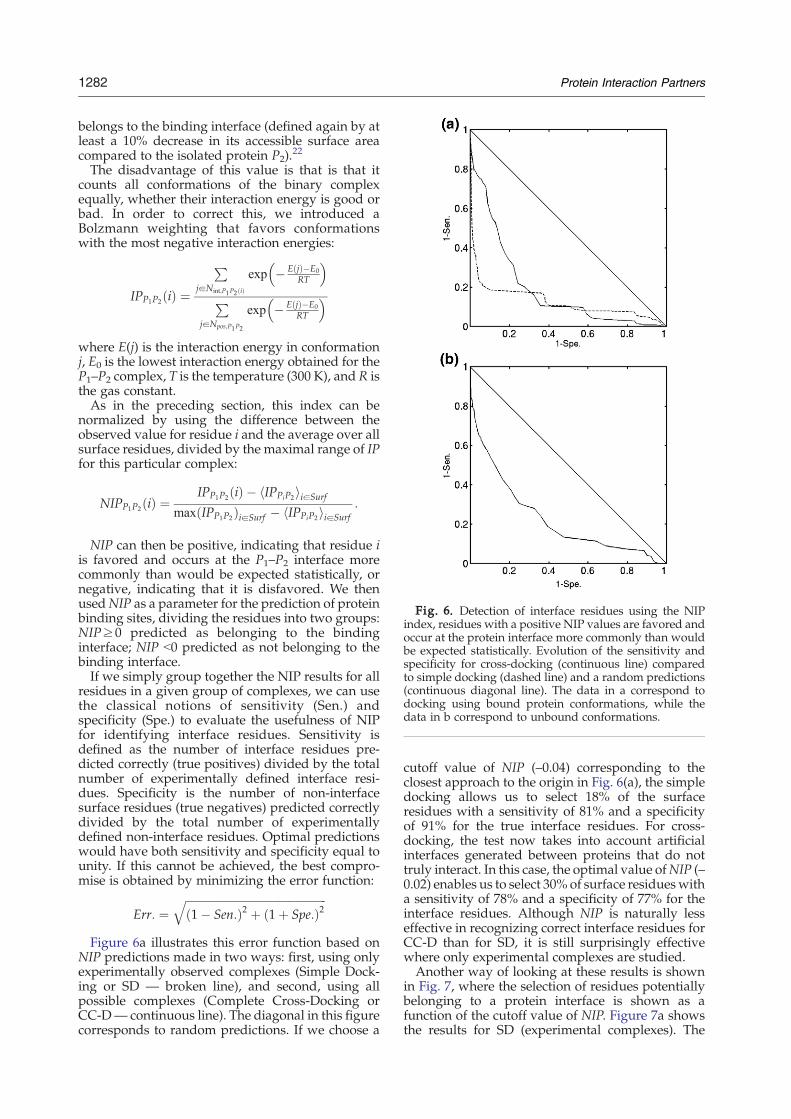
Fig. 6. Detection of interface residues using the NIPindex, residues with a positive NIP values are favored andoccur at the protein interface more commonly than wouldbe expected statistically. Evolution of the sensitivity andspecificity for cross-docking (continuous line) comparedto simple docking (dashed line) and a random predictions(continuous diagonal line). The data in a correspond todocking using bound protein conformations, while thedata in b correspond to unbound conformations.


belongs to the binding interface (defined again by atleast a 10% decrease in its accessible surface areacompared to the isolated protein P2).

22

The disadvantage of this value is that is that itcounts all conformations of the binary complexequally, whether their interaction energy is good orbad. In order to correct this, we introduced aBolzmann weighting that favors conformationswith the most negative interaction energies:

IPP1P2 ið Þ ¼

PjaNint;P1P2ðiÞ

exp � EðjÞ�E0RT

� �P

jaNpos;P1P2

exp � EðjÞ�E0RT

� �

where E(j) is the interaction energy in conformationj, E0 is the lowest interaction energy obtained for theP1–P2 complex, T is the temperature (300 K), and R isthe gas constant.As in the preceding section, this index can be

normalized by using the difference between theobserved value for residue i and the average over allsurface residues, divided by the maximal range of IPfor this particular complex:

NIPP1P2 ið Þ ¼ IPP1P2ðiÞ � hIPPiP2iiaSurf

maxðIPP1P2ÞiaSurf � hIPPiP2iiaSurf:

NIP can then be positive, indicating that residue iis favored and occurs at the P1–P2 interface morecommonly than would be expected statistically, ornegative, indicating that it is disfavored. We thenusedNIP as a parameter for the prediction of proteinbinding sites, dividing the residues into two groups:NIP≥0 predicted as belonging to the bindinginterface; NIP b0 predicted as not belonging to thebinding interface.If we simply group together the NIP results for all

residues in a given group of complexes, we can usethe classical notions of sensitivity (Sen.) andspecificity (Spe.) to evaluate the usefulness of NIPfor identifying interface residues. Sensitivity isdefined as the number of interface residues pre-dicted correctly (true positives) divided by the totalnumber of experimentally defined interface resi-dues. Specificity is the number of non-interfacesurface residues (true negatives) predicted correctlydivided by the total number of experimentallydefined non-interface residues. Optimal predictionswould have both sensitivity and specificity equal tounity. If this cannot be achieved, the best compro-mise is obtained by minimizing the error function:

Err: ¼ffiffiffiffiffiffiffiffiffiffiffiffiffiffiffiffiffiffiffiffiffiffiffiffiffiffiffiffiffiffiffiffiffiffiffiffiffiffiffiffiffiffiffiffiffiffiffiffiffiffiffið1� Sen:Þ2 þ ð1þ Spe:Þ2

qFigure 6a illustrates this error function based on

NIP predictions made in two ways: first, using onlyexperimentally observed complexes (Simple Dock-ing or SD — broken line), and second, using allpossible complexes (Complete Cross-Docking orCC-D— continuous line). The diagonal in this figurecorresponds to random predictions. If we choose a

cutoff value of NIP (–0.04) corresponding to theclosest approach to the origin in Fig. 6(a), the simpledocking allows us to select 18% of the surfaceresidues with a sensitivity of 81% and a specificityof 91% for the true interface residues. For cross-docking, the test now takes into account artificialinterfaces generated between proteins that do nottruly interact. In this case, the optimal value ofNIP (–0.02) enables us to select 30% of surface residueswitha sensitivity of 78% and a specificity of 77% for theinterface residues. Although NIP is naturally lesseffective in recognizing correct interface residues forCC-D than for SD, it is still surprisingly effectivewhere only experimental complexes are studied.Another way of looking at these results is shown

in Fig. 7, where the selection of residues potentiallybelonging to a protein interface is shown as afunction of the cutoff value of NIP. Figure 7a showsthe results for SD (experimental complexes). The

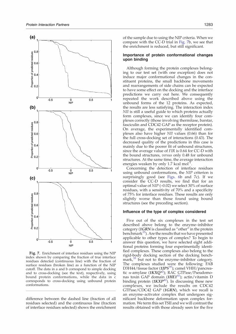
Fig. 7. Enrichment of interface residues using the NIPindex shown by comparing the fraction of true interfaceresidues detected (continuous line) with the fraction ofsurface residues (broken line) as a function of the NIPcutoff. The data in a and b correspond to simple dockingand to cross-docking (see the text), respectively, usingbound protein conformations, while the data in ccorresponds to cross-docking using unbound proteinconformations.


difference between the dashed line (fraction of allresidues selected) and the continuous line (fractionof interface residues selected) shows the enrichment

of the sample due to using the NIP criteria. Whenwecompare with the CC-D trial in Fig. 7b, we see thatthe enrichment is reduced, but still significant.

Importance of protein conformational changesupon binding

Although forming the protein complexes belong-ing to our test set (with one exception) does notinduce major conformational changes in the con-stituent proteins, the small backbone movementsand rearrangements of side chains can be expectedto have some effect on the docking and the interfacepredictions we carry out here. We consequentlyrepeated the work described above using theunbound forms of the 12 proteins. As expected,the results are less satisfying. The interaction indexNII is still a useful guide to which proteins actuallyform complexes, since we can identify four com-plexes correctly (those involving thermitase, barstar,fasciculin and CDC42 GAP as the receptor protein).On average, the experimentally identified com-plexes also have higher NII values (0.66) than forthe full cross-docking set of interactions (0.43). Thedecreased quality of the predictions in this case ismainly due to the poorer fit of unbound structures,since the average value of FIR is 0.64 for CC-D withthe bound structures, versus only 0.48 for unboundstructures. At the same time, the average interactionenergies weaken by only 1.7 kcal mol-1.Concerning the detection of interface residues

using unbound conformations, the NIP criterion issurprisingly good (see Figs. 6b and 7c). If weconsider the CC-D results, we find that for anoptimal value ofNIP (–0.02) we select 30% of surfaceresidues, with a sensitivity of 70% and a specificityof 75% for interface residues. These results are onlyslightly worse than those found using boundstructures (see the preceding section).

Influence of the type of complex considered

Five out of the six complexes in the test setdescribed above belong to the enzyme–inhibitorcategory (1GRN is classified as “other” in the proteinbenchmark35). Are the results thatwe have presentedapplicable to other types of complex? To begin toanswer this question, we have selected eight addi-tional proteins forming four experimentally identi-fied complexes. These complexes also belong to therigid-body docking section of the docking bench-mark,35 but not to the enzyme–inhibitor category.The complexes studied were the following: FABD3H44/tissue factor (1JPS39); camel VHH/pancrea-tic α-amylase (1KXQ40); RAC GTPase/Pseudomo-nas toxin GAP domain (1HE141); actin/vitamin Dbinding protein (1KXP42). In discussing these newcomplexes, we include the results on CDC42GTPase/CDC42 GAP (1GRN), which we recall isan enzyme–activator complex that undergoes sig-nificant backbone deformation upon complex for-mation.We term this set TSII andwewill contrast theresults obtained with those already seen for the five


enzyme–inhibitor complexes already discussed(TSI), that is, 1BRS, 2PTC, 1FSS, 2TEC and 1UGH.This choice yields two test sets involving ten proteinseach.We performed a CC-D trial on the TSII set in the

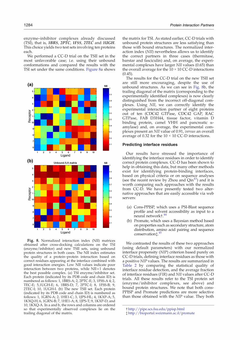
most unfavorable case; i.e. using their unboundconformations and compared the results with theTSI set under the same conditions. Figure 8a shows

Fig. 8. Normalized interaction index (NII) matricesobtained after cross-docking calculations on the TSI(enzyme/inhibitor) and new TSII sets, using unboundprotein structures in both cases. The NII index estimatesthe quality of a protein–protein interaction based oncorrect residues appearing at the interface combined withgood interaction energies. Low NII values indicate poorinteraction between two proteins, while NII=1 denotesthe best possible complex. (a) TSI enzyme/inhibitor set.Each protein (indicated by its PDB code and chain ID) isnumbered as follows: 1, 1BRS-A; 2, 2PTC-E; 3, 1FSS-A 4; 2,TEC-E; 5,1UGH-E; 6, 1BRS-D; 7, 2PTC-I; 8, 1FSS-B; 9,2TEC-I; 10, 1UGH-I. (b) The new TSII set. Each protein(indicated by its PDB code and chain ID) is numbered asfollows: 1, 1GRN-A; 2, 1HE1-C; 3, 1JPS-HL; 4, 1KXP-A; 5,1KXQ-H; 6, 1GRN-B; 7, 1HE1-A; 8, 1JPS-T; 9, 1KXP-D; and10, 1KXQ-A. In a and b, the rows and columns are orderedso that experimentally observed complexes lie on thetrailing diagonal of the matrix.

the matrix for TSI. As stated earlier, CC-D trials withunbound protein structures are less satisfying thanthose with bound structures. The normalized inter-action index (NII) nevertheless allows us to identifythe correct partners in three cases (thermitase,barstar and fasciculin) and, on average, the experi-mental complexes have larger NII values (0.65) thanthe overall average for the 10 × 10 CC-D interactions(0.45).The results for the CC-D trial on the new TSII set

are still more encouraging, despite the use ofunbound structures. As we can see in Fig. 8b, thetrailing diagonal of the matrix (corresponding to theexperimentally identified complexes) is now clearlydistinguished from the incorrect off-diagonal com-plexes. Using NII, we can correctly identify theexperimental interaction partner of eight proteinsout of ten (CDC42 GTPase, CDC42 GAP, RACGTPase, FAB D3H44, tissue factor, vitamin Dbinding protein, camel VHH and pancreatic α-amylase) and, on average, the experimental com-plexes present an NII value of 0.91, versus an overallaverage of 0.32 for the 10 × 10 CC-D interactions.

Predicting interface residues

Our results have stressed the importance ofidentifying the interface residues in order to identifycorrect protein complexes. CC-D has been shown tohelp in obtaining this data, but many other methodsexist for identifying protein-binding interfaces,based on physical criteria or on sequence analyses(see the recent review by Zhou and Qin43) and it isworth comparing such approaches with the resultsfrom CC-D. We have presently tested two alter-native approaches that are easily accessible via webservers:

(a) Cons-PPISP, which uses a PSI-Blast sequenceprofile and solvent accessibility as input to aneural network†.44

(b) Promate, which uses a Bayesian method basedon properties such as secondary structure, atomdistribution, amino acid pairing and sequenceconservation‡.45

We contrasted the results of these two approaches(using default parameters) with our normalizedinterface propensity (NIP) criterion based purely onCC-D trials, defining interface residues as those witha positiveNIP values. The results are summarized inTable 2 by comparing the statistical quality ofinterface residue detection, and the average fractionof interface residues (FIR) and NII values after CC-Dtrials. All these results refer to the TSI protein set(enzyme/inhibitor complexes, see above) andbound protein structures. We note that both cons-PPISP and Promate predictions are more selectivethan those obtained with the NIP value. They both

†http://pipe.scs.fsu.edu/ppisp.html‡http://bioportal.weizmann.ac.il/promate

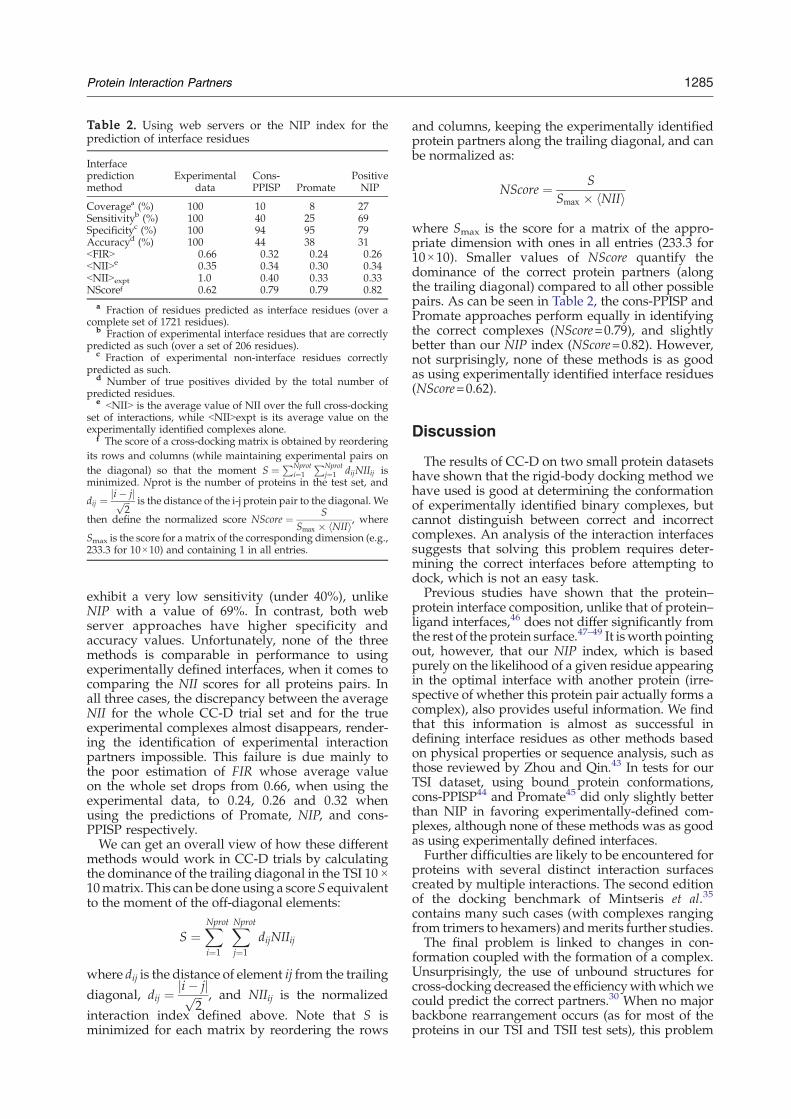
Table 2. Using web servers or the NIP index for theprediction of interface residues

Interfacepredictionmethod

Experimentaldata

Cons-PPISP Promate

PositiveNIP

Coveragea (%) 100 10 8 27Sensitivityb (%) 100 40 25 69Specificityc (%) 100 94 95 79Accuracyd (%) 100 44 38 31bFIRN 0.66 0.32 0.24 0.26bNIINe 0.35 0.34 0.30 0.34bNIINexpt 1.0 0.40 0.33 0.33NScoref 0.62 0.79 0.79 0.82

a Fraction of residues predicted as interface residues (over acomplete set of 1721 residues).

b Fraction of experimental interface residues that are correctlypredicted as such (over a set of 206 residues).

c Fraction of experimental non-interface residues correctlypredicted as such.

d Number of true positives divided by the total number ofpredicted residues.

e bNIIN is the average value of NII over the full cross-dockingset of interactions, while bNIINexpt is its average value on theexperimentally identified complexes alone.

f The score of a cross-docking matrix is obtained by reorderingits rows and columns (while maintaining experimental pairs onthe diagonal) so that the moment S ¼PNprot

i¼1

PNprotj¼1 dijNIIij is

minimized. Nprot is the number of proteins in the test set, and

dij ¼ ji� jjffiffiffi2

p is the distance of the i-j protein pair to the diagonal. We

then define the normalized score NScore ¼ SSmax � hNIIi, where

Smax is the score for a matrix of the corresponding dimension (e.g.,233.3 for 10×10) and containing 1 in all entries.


exhibit a very low sensitivity (under 40%), unlikeNIP with a value of 69%. In contrast, both webserver approaches have higher specificity andaccuracy values. Unfortunately, none of the threemethods is comparable in performance to usingexperimentally defined interfaces, when it comes tocomparing the NII scores for all proteins pairs. Inall three cases, the discrepancy between the averageNII for the whole CC-D trial set and for the trueexperimental complexes almost disappears, render-ing the identification of experimental interactionpartners impossible. This failure is due mainly tothe poor estimation of FIR whose average valueon the whole set drops from 0.66, when using theexperimental data, to 0.24, 0.26 and 0.32 whenusing the predictions of Promate, NIP, and cons-PPISP respectively.We can get an overall view of how these different

methods would work in CC-D trials by calculatingthe dominance of the trailing diagonal in the TSI 10 ×10matrix. This can be done using a score S equivalentto the moment of the off-diagonal elements:

S ¼XNprot

i¼1

XNprot

j¼1

dijNIIij

where dij is the distance of element ij from the trailing

diagonal, dij ¼ ji� jjffiffiffi2

p , and NIIij is the normalized

interaction index defined above. Note that S isminimized for each matrix by reordering the rows

and columns, keeping the experimentally identifiedprotein partners along the trailing diagonal, and canbe normalized as:

NScore ¼ SSmax � hNIIi

where Smax is the score for a matrix of the appro-priate dimension with ones in all entries (233.3 for10×10). Smaller values of NScore quantify thedominance of the correct protein partners (alongthe trailing diagonal) compared to all other possiblepairs. As can be seen in Table 2, the cons-PPISP andPromate approaches perform equally in identifyingthe correct complexes (NScore=0.79), and slightlybetter than our NIP index (NScore=0.82). However,not surprisingly, none of these methods is as goodas using experimentally identified interface residues(NScore=0.62).

Discussion

The results of CC-D on two small protein datasetshave shown that the rigid-body docking method wehave used is good at determining the conformationof experimentally identified binary complexes, butcannot distinguish between correct and incorrectcomplexes. An analysis of the interaction interfacessuggests that solving this problem requires deter-mining the correct interfaces before attempting todock, which is not an easy task.Previous studies have shown that the protein–

protein interface composition, unlike that of protein–ligand interfaces,46 does not differ significantly fromthe rest of the protein surface.47–49 It isworth pointingout, however, that our NIP index, which is basedpurely on the likelihood of a given residue appearingin the optimal interface with another protein (irre-spective of whether this protein pair actually forms acomplex), also provides useful information. We findthat this information is almost as successful indefining interface residues as other methods basedon physical properties or sequence analysis, such asthose reviewed by Zhou and Qin.43 In tests for ourTSI dataset, using bound protein conformations,cons-PPISP44 and Promate45 did only slightly betterthan NIP in favoring experimentally-defined com-plexes, although none of these methods was as goodas using experimentally defined interfaces.Further difficulties are likely to be encountered for

proteins with several distinct interaction surfacescreated by multiple interactions. The second editionof the docking benchmark of Mintseris et al.35

contains many such cases (with complexes rangingfrom trimers to hexamers) andmerits further studies.The final problem is linked to changes in con-

formation coupled with the formation of a complex.Unsurprisingly, the use of unbound structures forcross-dockingdecreased the efficiencywithwhichwecould predict the correct partners.30 When no majorbackbone rearrangement occurs (as for most of theproteins in our TSI and TSII test sets), this problem

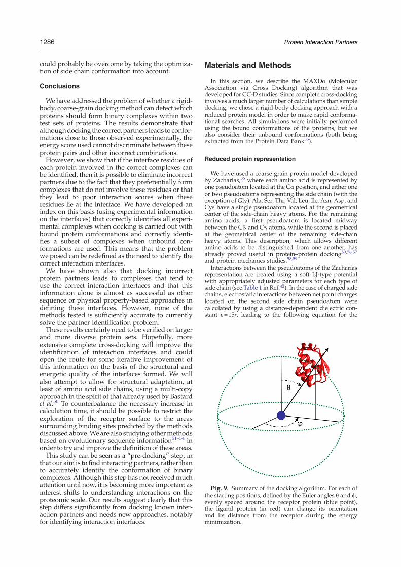
Fig. 9. Summary of the docking algorithm. For each ofthe starting positions, defined by the Euler angles θ and ϕ,evenly spaced around the receptor protein (blue point),the ligand protein (in red) can change its orientationand its distance from the receptor during the energyminimization.


could probably be overcome by taking the optimiza-tion of side chain conformation into account.

Conclusions

Wehave addressed the problemofwhether a rigid-body, coarse-grain dockingmethod can detect whichproteins should form binary complexes within twotest sets of proteins. The results demonstrate thatalthoughdocking the correct partners leads to confor-mations close to those observed experimentally, theenergy score used cannot discriminate between theseprotein pairs and other incorrect combinations.However, we show that if the interface residues of

each protein involved in the correct complexes canbe identified, then it is possible to eliminate incorrectpartners due to the fact that they preferentially formcomplexes that do not involve these residues or thatthey lead to poor interaction scores when theseresidues lie at the interface. We have developed anindex on this basis (using experimental informationon the interfaces) that correctly identifies all experi-mental complexes when docking is carried out withbound protein conformations and correctly identi-fies a subset of complexes when unbound con-formations are used. This means that the problemwe posed can be redefined as the need to identify thecorrect interaction interfaces.We have shown also that docking incorrect

protein partners leads to complexes that tend touse the correct interaction interfaces and that thisinformation alone is almost as successful as othersequence or physical property-based approaches indefining these interfaces. However, none of themethods tested is sufficiently accurate to currentlysolve the partner identification problem.These results certainly need to be verified on larger

and more diverse protein sets. Hopefully, moreextensive complete cross-docking will improve theidentification of interaction interfaces and couldopen the route for some iterative improvement ofthis information on the basis of the structural andenergetic quality of the interfaces formed. We willalso attempt to allow for structural adaptation, atleast of amino acid side chains, using a multi-copyapproach in the spirit of that already used by Bastardet al.50 To counterbalance the necessary increase incalculation time, it should be possible to restrict theexploration of the receptor surface to the areassurrounding binding sites predicted by the methodsdiscussed above.We are also studying othermethodsbased on evolutionary sequence information51–54 inorder to try and improve the definition of these areas.This study can be seen as a “pre-docking” step, in

that our aim is to find interacting partners, rather thanto accurately identify the conformation of binarycomplexes. Although this step has not receivedmuchattention until now, it is becomingmore important asinterest shifts to understanding interactions on theproteomic scale. Our results suggest clearly that thisstep differs significantly from docking known inter-action partners and needs new approaches, notablyfor identifying interaction interfaces.

Materials and Methods

In this section, we describe the MAXDo (MolecularAssociation via Cross Docking) algorithm that wasdeveloped for CC-D studies. Since complete cross-dockinginvolves a much larger number of calculations than simpledocking, we chose a rigid-body docking approach with areduced protein model in order to make rapid conforma-tional searches. All simulations were initially performedusing the bound conformations of the proteins, but wealso consider their unbound conformations (both beingextracted from the Protein Data Bank55).

Reduced protein representation

We have used a coarse-grain protein model developedby Zacharias,56 where each amino acid is represented byone pseudoatom located at the Cα position, and either oneor two pseudoatoms representing the side chain (with theexception of Gly). Ala, Ser, Thr, Val, Leu, Ile, Asn, Asp, andCys have a single pseudoatom located at the geometricalcenter of the side-chain heavy atoms. For the remainingamino acids, a first pseudoatom is located midwaybetween the Cβ and Cγ atoms, while the second is placedat the geometrical center of the remaining side-chainheavy atoms. This description, which allows differentamino acids to be distinguished from one another, hasalready proved useful in protein–protein docking50,56,57

and protein mechanics studies.58,59

Interactions between the pseudoatoms of the Zachariasrepresentation are treated using a soft LJ-type potentialwith appropriately adjusted parameters for each type ofside chain (see Table 1 in Ref.42). In the case of charged sidechains, electrostatic interactions between net point chargeslocated on the second side chain pseudoatom werecalculated by using a distance-dependent dielectric con-stant ε=15r, leading to the following equation for the


interaction energy of the pseudoatom pair i,j at distancerij:

Eij ¼Bij

r8ij� Cij

r6ij

!þ qiqj15r2ij

where Bij and Cij are the repulsive and attractive LJ-typeparameters, respectively, and qi and qjare the charges ofthe pseudoatoms i and j.

Systematic docking simulations

Our systematic docking algorithm (Fig. 9) was derivedfrom the ATTRACT protocol of Zacharias56 and uses amultiple energy minimization scheme. For each pair ofproteins, the first molecule (called receptor) was fixed inspace, while the second (termed the ligand protein) wasused as a probe and placed at multiple positions on thesurface of the receptor. The distance of the probe from thereceptor was chosen so that no pair of probe-receptorpseudoatoms came closer than 6 Å. Starting probepositions were randomly created around the receptorsurface with a density of one position per 10 Å2, and foreach starting position, 210 different ligand orientationswere generated, resulting in a total number of startconfigurations ranging from 95,000 to 450,000 dependingon the size of the receptor.During each energy minimization, the ligand protein

was kept at a given location over the surface of thereceptor protein by using a harmonic restraint to maintainits center of mass on a vector passing through the center ofmass of the receptor protein. The direction of this vectorwas defined by two Euler angles θ and φ, (where θ = φ, =0° was chosen to pass through the center of the bindinginterface of the receptor protein) as shown in Fig. 9. Byvarying the Euler angles from 0°→360° and 0°→180°,respectively, it was possible to sample interactions evenlyover the complete surface of the receptor and to representits binding potential using 2D energy maps (each pointcorresponding to the best ligand orientation for the chosenθ/φ pair).

Computational implementation

Each energy minimization for a pair of interactingproteins takes typically 15 s on a single 2 GHz processor.As stated above, 100,000 ∼ 450,000 minimizations arerequired to probe all possible interaction conformations,depending on the size of the interacting proteins. Thiswould require many days of computation on a singleprocessor. Happily, each minimization is independent ofthe others and this problem therefore belongs to the so-called "embarrassingly parallel" category and is perfectlyadapted to petaflop machines with very large numbers ofprocessors, or to grid calculations. In the present case, theCC-D trials have been performed on the DECRYTHONuniversity grid§, where the docking of a single proteinpair took between 5 h and two days (depending on thesize of the proteins and the grid availability). The MAXDoprogram is currently being refined and it is expected that itwill be possible to gain a factor of 4–5. Larger CC-D trialswill be carried out using the World Community Grid∥whose massive computational power will enable us toscan CC-D sets involving thousands of proteins.

§www.decrypthon.fr∥www.worldcommunitygrid.org

Acknowledgements

This work was carried out in the framework of theDECRYPTHON Project, set up by the CNRS (CentreNational de la Recherche Scientifique), the AFM(French Muscular Distrophy Association) and IBM.The cross-docking simulations were performed onthe Decrypthon University Grid, and we thankRaphaël Bolze for adapting our docking program foruse on this grid. S.S.-M. thanks the AFM for one yearof post-doctoral funding during which part of thiswork was carried out.

References

1. Ellis, R. J. & Minton, A. P. (2003). Cell biology - join thecrowd. Nature, 425, 27–28.

2. Minton, A. P. (2000). Implications of macromolecularcrowding for protein assembly. Curr. Opin. Struct. Biol.10, 34–39.

3. Deeds, E. J., Ashenberg,O.,Gerardin, J. & Shakhnovich,E. I. (2007). Robust protein-protein interactions incrowded cellular environments. Proc. Natl Acad. Sci.USA, 104, 14952–14957.

4. Rigaut, G., Shevchenko, A., Rutz, B., Wilm, M.,Mann, M. & Seraphin, B. (1999). A generic proteinpurification method for protein complex character-ization and proteome exploration. Nature Biotechnol.17, 1030–1032.

5. Uetz, P., Giot, L., Cagney, G., Mansfield, T. A., Judson,R. S., Knight, J. R. et al. (2000). A comprehensiveanalysis of protein-protein interactions in Saccharo-myces cerevisiae. Nature, 403, 623–627.

6. Ito, T., Chiba, T., Ozawa, R., Yoshida, M., Hattori, M.& Sakaki, Y. (2001). A comprehensive two-hybridanalysis to explore the yeast protein interactome.Proc. Natl Acad. Sci. USA, 98, 4569–4574.

7. Ho, Y., Gruhler, A., Heilbut, A., Bader, G. D., Moore,L., Adams, S. L. et al. (2002). Systematic identificationof protein complexes in Saccharomyces cerevisiae bymass spectrometry. Nature, 415, 180–183.

8. Gavin, A. C., Bosche, M., Krause, R., Grandi, P.,Marzioch, M., Bauer, A. et al. (2002). Functionalorganization of the yeast proteome by systematicanalysis of protein complexes. Nature, 415, 141–147.

9. Xenarios, L. & Eisenberg, D. (2001). Protein interactiondatabases. Curr. Opin. Biotechnol. 12, 334–339.

10. Shoemaker, B. A. & Panchenko, A. R. (2007).Deciphering protein-protein interactions. Part I.Experimental techniques and databases. Plos Comput.Biol. 3, 337–344.

11. Bader, G. D., Donaldson, I., Wolting, C., Ouellette, B.F. F., Pawson, T. & Hogue, C. W. V. (2001). BIND - thebiomolecular interaction network database. NucleicAcids Res. 29, 242–245.

12. Shoemaker, B. A. & Panchenko, A. R. (2007). Decipher-ing protein-protein interactions. Part II. Computa-tional methods to predict protein and domaininteraction partners. Plos Comput. Biol. 3, 595–601.

13. Deane, C. M., Salwinski, L., Xenarios, I. & Eisenberg,D. (2002). Protein interactions - Two methods forassessment of the reliability of high throughputobservations. Mol. Cell. Proteomics, 1, 349–356.

14. Levinthal, C., Wodak, S. J., Kahn, P. & Dadivanian,A. K. (1975). Hemoglobin interaction in sickle-cellfibers .1. Theoretical approaches to molecular con-tacts. Proc. Natl Acad. Sci. USA, 72, 1330–1334.


15. Wodak, S. J. & Janin, J. (1978). Computer analysis ofprotein–protein interaction. J. Mol. Biol. 124, 323–342.

16. Jones, S. & Thornton, J. M. (1996). Principles of protein-protein interactions.Proc. Natl Acad. Sci. USA, 93, 13–20.

17. Mendez, R., Leplae, R., Lensink, M. F. & Wodak, S. J.(2005). Assessment of CAPRI predictions in rounds 3-5 shows progress in docking procedures. Proteins:Struct. Funct. Bioinform. 60, 150–169.

18. Carter, P., Lesk, V. I., Islam, S. A. & Sternberg, M. J. E.(2005). Protein-protein docking using, 3, 281–288.

19. Bahadur, R. P. & Zacharias, M. (2008). The interfaceof protein-protein complexes: Analysis of contactsand prediction of interactions. Cell. Mol. Life Sci. 65,1059–1072.

20. Lesk, V. I. & Sternberg, M. J. E. (2008). 3D-Garden: asystem for modelling proteinprotein complexes basedon conformational refinement of ensembles generatedwith the marching cubes algorithm. Bioinformatics, 24,1137–1144.

21. Lensink, M. F., Mendez, R. & Wodak, S. J. (2007).Docking and scoring protein complexes: CAPRI 3rdedition. Proteins: Struct. Funct. Bioinform. 69, 704–718.

22. Fernandez-Recio, J., Totrov, M. & Abagyan, R. (2004).Identification of protein-protein interaction sites fromdocking energy landscapes. J. Mol. Biol. 335, 843–865.

23. Elcock, A. H. (2002). Atomistic Simulations ofcompetition between substrates binding to anenzyme. Biophys. J. 82, 2326–2332.

24. Macchiarulo, A., Nobeli, I. & Thornton, J. M. (2004).Ligand selectivity and competition between enzymesin silico. Nature Biotechnol. 22, 1039–1045.

25. Yang, J. M. & Chen, C. C. (2004). GEMDOCK: Ageneric evolutionary method for molecular docking.Proteins: Struct. Funct. Bioinform. 55, 288–304.

26. Sotriffer, C. A. & Dramburg, I. (2005). “In situ cross-docking” to simultaneously address multiple targets.J. Med. Chem. 48, 3122–3125.

27. Meiler, J. & Baker, D. (2006). ROSETTALIGAND:protein-small molecule docking with full side-chainflexibility. Proteins: Struct. Funct. Bioinform. 65, 538–548.

28. Bottegoni, G., Kufareva, I., Totrov, M. & Abagyan, R.(2008). A new method for ligand docking to flexiblereceptors by dual alanine scanning and refinement(SCARE). J. Comput.Aided Mol. Des. 22, 311–325.

29. Claussen, H., Buning, C., Rarey, M. & Lengauer, T.(2001). FlexE: efficient molecular docking consideringprotein structure variations. J. Mol. Biol. 308, 377–395.

30. Smith, G. R., Sternberg, M. J. E. & Bates, P. A. (2005).The relationship between the flexibility of proteinsand their conformational states on forming protein–protein complexes with an application to protein-protein docking. J. Mol. Biol. 347, 1077–1101.

31. Zhao, Y. & Sanner, M. F. (2007). FLIPDock: Dockingflexible ligands into flexible receptors. Proteins: Struct.Funct. Bioinform. 68, 726–737.

32. Krol, M., Chaleil, R. A. G., Tournier, A. T. & Bates, P. A.(2007). Implicit flexibility in protein docking: Cross-docking and local refinement. Proteins: Struct. Funct.Bioinform. 69, 750–757.

33. Lee, H. S., Choi, J., Kufareva, I., Abagyan, R., Filikov,A., Yang, Y. & Yoon, S. (2008). Optimization of highthroughput virtual screening by combining shape-matching and docking methods. J. Chem. Informat.Model. 48, 489–497.

34. Chen, R., Mintseris, J., Janin, J. & Weng, Z. P. (2003). Aprotein-protein docking benchmark. Proteins: Struct.Funct. Genet. 52, 88–91.

35. Mintseris, J., Wiehe, K., Pierce, B., Anderson, R., Chen,R., Janin, J. & Weng, Z. P. (2005). Protein-protein

docking benchmark 2.0: An update. Proteins: Struct.Funct. Bioinform. 60, 214–216.

36. Brooijmans, N., Sharp, K. A. & Kuntz, I. D. (2002).Stability of macromolecular complexes. Proteins:Struct. Funct. Genet. 48, 645–653.

37. Bahadur, R. P., Chakrabarti, P., Rodier, F. & Janin, J.(2004). A dissection of specific and non-specificprotein – protein interfaces. J. Mol. Biol. 336,943–955.

38. Hubbard, S. J. (1992).ACCESS: a program for calculatingaccessibilities, Department of Biochemistry and MolecularBiology. University College of London, .

39. Faelber, K., Kirchhofer, D., Presta, L., Kelley, R. F. &Muller, Y. A. (2001). The 1.85 Å resolution crystalstructures of tissue factor in complex with humanizedFab D3h44 and of free humanized Fab D3h44:Revisiting the solvation of antigen combining sites.J. Mol. Biol. 313, 83–97.

40. Desmyter, A., Spinelli, S., Payan, F., Lauwereys, M.,Wyns, L., Muyldermans, S. & Cambillau, C. (2002).Three Camelid VHH domains in complex withporcine pancreatic alpha-amylase - Inhibition andversatility of binding topology. J. Biol. Chem. 277,23645–23650.

41. Wurtele, M., Wolf, E., Pederson, K. J., Buchwald, G.,Ahmadian, M. R., Barbieri, J. T. & Wittinghofer, A.(2001). How the Pseudomonas aeruginosa ExoS toxindownregulates Rac. Nature Struct. Biol. 8, 23–26.

42. Otterbein, L. R., Cosio, C., Graceffa, P. & Dominguez,R. (2002). Crystal structures of the vitamin D-bindingprotein and its complex with actin: Structural basis ofthe actin-scavenger system. Proc. Natl. Acad. of Sci.USA, 99, 8003–8008.

43. Zhou, H. X. & Qin, S. B. (2007). Interaction-siteprediction for protein complexes: a critical assess-ment. Bioinformatics, 23, 2203–2209.

44. Chen, H. L. & Zhou, H. X. (2005). Prediction ofinterface residues in protein-protein complexes by aconsensus neural network method: Test againstNMR data. Proteins: Struct. Funct. Bioinform. 61,21–35.

45. Neuvirth, H., Raz, R. & Schreiber, G. (2004). ProMate:a structure based prediction program to identify thelocation of protein-protein binding sites. J. Mol. Biol.338, 181–199.

46. Burgoyne, N. J. & Jackson, R. M. (2006). Predictingprotein interaction sites: binding hot-spots in protein-protein and protein-ligand interfaces. Bioinformatics,22, 1335–1342.

47. Chothia, C. & Janin, J. (1975). Principles of protein-protein recognition. Nature, 256, 705–708.

48. Janin, J. & Chothia, C. (1990). The structure ofprotein-protein recognition sites. J. Biol. Chem. 265,16027–16030.

49. Lo Conte, L., Chothia, C. & Janin, J. (1999). The atomicstructure of protein-protein recognition sites. J. Mol.Biol. 285, 2177–2198.

50. Bastard, K., Prevost, C. & Zacharias, M. (2006).Accounting for loop flexibility during protein-protein docking. Proteins: Struct. Funct. Bioinform.62, 956–969.

51. Dong, Q. W., Wang, X. L., Lin, L. & Guan, Y. (2007).Exploiting residue-level and profile-level interfacepropensities for usage in binding sites prediction ofproteins. BMC Bioinformat. 8.

52. Lichtarge, O., Bourne, H. R. & Cohen, F. E. (1996).An evolutionary trace method defines bindingsurfaces common to protein families. J. Mol. Biol.257, 342–358.


53. Lichtarge, O. & Sowa, M. E. (2002). Evolutionarypredictions of binding surfaces and interactions. Curr.Opin. Struct. Biol. 12, 21–27.

54. Mihalek, I., Res, I. & Lichtarge, O. (2006). Evolutionarytrace report_maker: a new type of service forcomparative analysis of proteins. Bioinformatics, 22,1656–1657.

55. Berman, H. M., Battistuz, T., Bhat, T. N., Bluhm, W. F.,Bourne, P. E., Burkhardt, K. et al. (2002). The ProteinData Bank. Acta Crystallogr. D, 58, 899–907.

56. Zacharias, M. (2003). Protein-protein docking with areduced protein model accounting for side-chainflexibility. Protein Sci. 12, 1271–1282.

57. Zacharias, M. (2005). ATTRAACT: protein-proteindocking in CAPRI using a reduced protein model.Proteins: Struct. Funct. Bioinform. 60, 252–256.

58. Sacquin-Mora, S. & Lavery, R. (2006). Investigatingthe local flexibility of functional residues in hemopro-teins. Biophys. J. 90, 2706–2717.

59. Sacquin-Mora, S., Laforet, E. & Lavery, R. (2007).Locating the active sites of enzymes using mechanicalproperties. Proteins: Struct. Funct. Bioinform. 67,350–359.

60. W. Humphrey, A. Dalke, K. Schulten, (1996). VMD:visual molecular dynamics, J. Mol. Graph. 14, 33–8,27–28.

identification of protein interaction partners and protein-protein interaction sites

Documents