aerospace

Article

Identification of In-Flight Wingtip Folding Effectson the Roll Characteristics of a Flexible Aircraft

Gaétan Dussart *, Sezsy Yusuf and Mudassir Lone

Dynamic Simulation and Control Group, School of Aerospace, Transport and Manufacturing, CranfieldUniversity, Bedfordshire MK43 0AL, UK; sezsy.yusuf@cranfield.ac.uk (S.Y.); m.m.lone@cranfield.ac.uk (M.L.)* Correspondence: g.x.dussart@cranfield.ac.uk

Received: 15 April 2019; Accepted: 24 May 2019; Published: 30 May 2019�����������������

Abstract: Wingtip folding is a means by which an aircraft’s wingspan can be extended, allowingdesigners to take advantage of the associated reduction in induced drag. This type of device canprovide other benefits if used in flight, such as flight control and load alleviation. In this paper,the authors present a method to develop reduced order flight dynamic models for in-flight wingtipfolding, which are suitable for implementation in real-time pilot-in-the-loop simulations. Aspectssuch as the impact of wingtip size and folding angle on aircraft roll dynamics are investigatedalong with failure scenarios using a time domain aeroservoelastic framework and an establishedsystem identification method. The process discussed in this paper helps remove the need for directconnection of complex physics based models to engineering flight simulators and the need fortedious programming of large look-up-tables in simulators. Instead, it has been shown that a genericpolynomial model for roll aeroderivatives can be used in small roll perturbation conditions tosimulate the roll characteristics of an aerodynamic derivative based large transport aircraft equippedwith varying fold hinge lines and tip deflections. Moreover, the effects of wing flexibility arealso considered.

Keywords: system identification; flight dynamics; folding wingtips; aeroservoelastic framework;lateral; flight simulation

1. Introduction

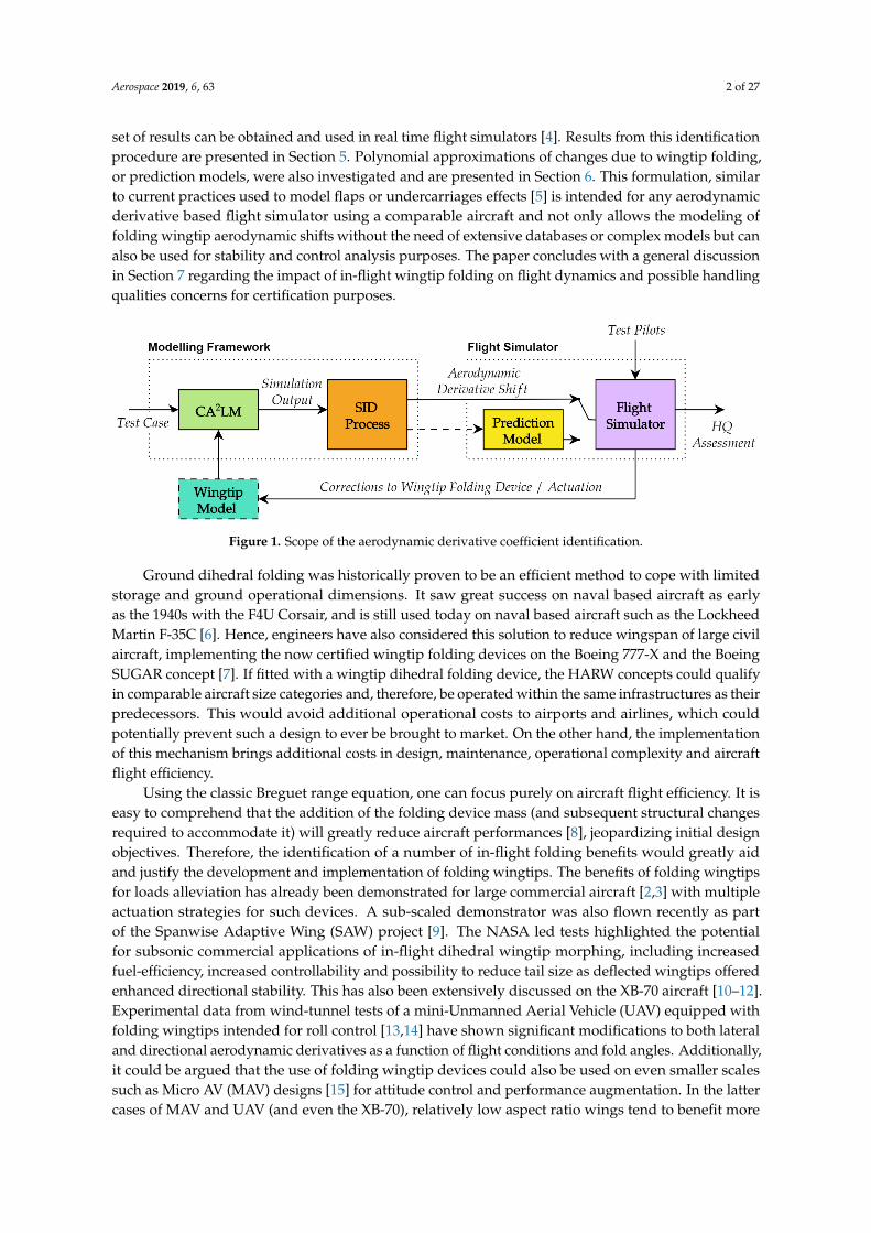
In the scope of a wider research project led at Cranfield University, the aim of this work wasto quantify the impact of a specific in-flight dihedral folding wingtips system on the lateral flightdynamics of a large generic civil aircraft. With aircraft handling qualities and pilot-in-the-loopsimulations in mind, this work focused on capturing roll damping and aileron effectiveness changeswith wingtip angle, quantities widely used by pilots for roll performance and lateral handling qualitiesanalysis. Figure 1 illustrates the logical link between the various elements of this research, from testcase definition, tool and method presentation, aerodynamic derivative identification and predictionmodel derivation.

The motivation behind this interest for in-flight folding wingtips is presented in the Introduction.Section 2 is dedicated to the kinematic and geometric description of the flared folding mechanism usedherein and past publications [1–3]. The device was implemented within the Cranfield AcceleratedAeroplane Loads Model (CA2LM), briefly presented in Section 3. This non-linear six degrees offreedom aircraft flight simulation environment was used to compute flight dynamic responses ofa morphing aircraft in various folding and flight conditions based on a physics based model ofthe folding wingtip system. A conventional systems identification method, described in Section 4,was then used to quantify the lateral aerodynamic derivatives of interest over a wide range of test cases(flight conditions and symmetric folding configurations). Thus, a more robust and widely applicable

Aerospace 2019, 6, 63; doi:10.3390/aerospace6060063 www.mdpi.com/journal/aerospace

Aerospace 2019, 6, 63 2 of 27

set of results can be obtained and used in real time flight simulators [4]. Results from this identificationprocedure are presented in Section 5. Polynomial approximations of changes due to wingtip folding,or prediction models, were also investigated and are presented in Section 6. This formulation, similarto current practices used to model flaps or undercarriages effects [5] is intended for any aerodynamicderivative based flight simulator using a comparable aircraft and not only allows the modeling offolding wingtip aerodynamic shifts without the need of extensive databases or complex models but canalso be used for stability and control analysis purposes. The paper concludes with a general discussionin Section 7 regarding the impact of in-flight wingtip folding on flight dynamics and possible handlingqualities concerns for certification purposes.

Figure 1. Scope of the aerodynamic derivative coefficient identification.

Ground dihedral folding was historically proven to be an efficient method to cope with limitedstorage and ground operational dimensions. It saw great success on naval based aircraft as earlyas the 1940s with the F4U Corsair, and is still used today on naval based aircraft such as the LockheedMartin F-35C [6]. Hence, engineers have also considered this solution to reduce wingspan of large civilaircraft, implementing the now certified wingtip folding devices on the Boeing 777-X and the BoeingSUGAR concept [7]. If fitted with a wingtip dihedral folding device, the HARW concepts could qualifyin comparable aircraft size categories and, therefore, be operated within the same infrastructures as theirpredecessors. This would avoid additional operational costs to airports and airlines, which couldpotentially prevent such a design to ever be brought to market. On the other hand, the implementationof this mechanism brings additional costs in design, maintenance, operational complexity and aircraftflight efficiency.

Using the classic Breguet range equation, one can focus purely on aircraft flight efficiency. It iseasy to comprehend that the addition of the folding device mass (and subsequent structural changesrequired to accommodate it) will greatly reduce aircraft performances [8], jeopardizing initial designobjectives. Therefore, the identification of a number of in-flight folding benefits would greatly aidand justify the development and implementation of folding wingtips. The benefits of folding wingtipsfor loads alleviation has already been demonstrated for large commercial aircraft [2,3] with multipleactuation strategies for such devices. A sub-scaled demonstrator was also flown recently as partof the Spanwise Adaptive Wing (SAW) project [9]. The NASA led tests highlighted the potentialfor subsonic commercial applications of in-flight dihedral wingtip morphing, including increasedfuel-efficiency, increased controllability and possibility to reduce tail size as deflected wingtips offeredenhanced directional stability. This has also been extensively discussed on the XB-70 aircraft [10–12].Experimental data from wind-tunnel tests of a mini-Unmanned Aerial Vehicle (UAV) equipped withfolding wingtips intended for roll control [13,14] have shown significant modifications to both lateraland directional aerodynamic derivatives as a function of flight conditions and fold angles. Additionally,it could be argued that the use of folding wingtip devices could also be used on even smaller scalessuch as Micro AV (MAV) designs [15] for attitude control and performance augmentation. In the lattercases of MAV and UAV (and even the XB-70), relatively low aspect ratio wings tend to benefit more

Aerospace 2019, 6, 63 3 of 27

from folding wingtips as control surfaces or directional stability enhancements whilst higher aspectratio may also see benefits directly on roll performances and potential loads alleviation applications.

In any case, these past findings and examples highlight that wingtip folding does have a significantimpact on aircraft flight dynamics. In other words, the response to pilot inputs or external disturbanceswill change with wingtip deflection. The amplitude of the shift in flight dynamic properties relativeto the baseline shape must therefore be quantified and assessed for certification, pilot training orfor the purpose of adequate flight control augmentation. Past work from the authors [1] presentedan initial discussion regarding the impact of airframe flexibility and wingtip dihedral folding ona large civil aircraft. For a smaller set of flight conditions, significant differences in lateral aerodynamicderivatives between rigid and flexible airframe simulations were outlined. The impact of wingtipfolding itself was also highlighted. These results were encouraging for certification, pilot training [4] oraugmentation purposes, as the shift in the aerodynamic derivatives was relatively small with foldingfor a device capable of significantly reducing span for ground operations. However, further work isneeded over a wider range of flight conditions and folding angles.

2. In-Flight Folding Wingtip Device Characteristics

The development and selection process of the folding wingtip device lays outside the scopeof this paper. However, the requirements can be summarized as follows: (a) significantly reduceaircraft wingspan during ground operations; (b) provide aerodynamic loads alleviation capability,both through controlled and soft failed (released) actuation; and (c) rely on conventional actuatorsfor wing folding (hydraulic or electric motors). As a result of prior studies, a hybrid twist-dihedralfolding system was adopted. Using a flared hinge line angle, the dihedral rotation of the wingtip leadsto an effective twist modification [2]. Thus, aerodynamic loads alleviation is achieved by reducingthe angle of attack or local twist of the aerofoil as wingtip is folded. A sketch of the device geometry isgiven in Figure 2a , where the hinge line is rotated around the vertical axis by a non-zero flare angleΛhinge shown in dark red. Hence, dihedral rotation leads to an effective twist angle modification,given by:

∆θwt = tan−1(

tan(Λhinge)× sin(Γwt))

(1)

where ∆θwt is the change in local twist angle due to the dihedral fold angle Γwt and hinge flare angleΛhinge as defined in Figure 2a. A geometrical derivation of Equation (1) is given Appendix A. A hingeline pointing outward on the leading edge effectively leads to a decrease in local angle of attack foran upward dihedral rotation. Symmetrically, an inward pointing hinge line leads to an increase in angleof attack with upward folding [2]. Twist angle evolutions for different hinge flare angles are illustratedin Figure 2b, with an emphasis on the flare angle Λhinge = 17◦ selected for this specific investigation.Note that the aerodynamic limitations of the aeroservoelastic framework and the maximum wingtipfolding angle used herein are included on the graph for illustrative purposes, showing that wingtiplocal angle of attack shift due to folding is kept below 10◦.

The actuation dynamics of the device are also a critical aspect of the design. The actuationdevice, which should be effective at both unloading the wing under excessive gust or maneuver loadsand restoring the wingtip after a high load incident, is not investigated here. The transient dynamicsof a release or failure are also not considered at this stage of the investigation. The device is assumedto fit within the profile without the needs of an additional fairing at the hinge line.

Aerospace 2019, 6, 63 4 of 27

(a) (b)

Figure 2. Flared dihedral folding wingtip mechanism: (a) sketch of the morphing wingtip geometry;and (b) local twist modification ∆θwt with Γwt and Λhinge.

3. Modeling the Wingtip in an Aeroservoelastic Framework

3.1. CA2LM Overview

The Cranfield Aircraft Accelerated Loads Model (CA2LM) framework [16,17] is an aeroservoelasticsimulation tool developed in MATLAB/Simulink and capable of near real-time simulations. It couplesboth linear structural model with unsteady aerodynamics in the time domain to couple aircraft flightdynamics with aeroelastics. Unsteady aerodynamics are based on a Modified Strip Theory, usingLeishmann [18] and Leishman–Beddoes [19] formulations, tail downwash calculations and coupledwith empirical fuselage, engine/nacelle and wing–body interaction modeling techniques fromEmpirical Scientific Data Units (ESDU). A modal approach is used to deform the complete aircraftstructure under aerodynamic and inertial loading. Updated Center of Gravity (CoG) positions areused to compute aircraft positions, velocities and accelerations in all six Degrees of Freedom (DoF)using common Equations of Motion (EoM). Aircraft position is used in both gravity and atmosphericmodels to complete the simulation environment. For a more detailed description of the framework,the reader is referred to the dedicated literature [16,17,20–23]. The Matlab/Simulink based tool canalso be used for handling qualities investigations, and was previously used to study realistic pilotmodels, effect of manual controls on flexible structures [24] and flight loads [25].

3.2. Aircraft Overview

The aircraft selected for this investigation is the Cranfield University AX-1 model, which is moreextensively described in past literature [16,17,20,21]. Additional geometric details of the aircraft aregiven in Appendix D. Figure 3 illustrates the beam–stick model used to model and compute aircraftstructural deformations, aerodynamic loading distribution and overall flight dynamics, with structuralnode (in grey), aerodynamic station distribution (profiles shown in blue), control surface position(shown in red) and different wingtip sizes.

Stiffness parameters of the wing structure are selected to emphasize the aeroservoelastic effectswithin the framework whilst keeping the behavior comparable to that of a large civil aircraft. Globalstructural damping is 3%. Both rigid and flexible structures are compared to assess the impact ofstructural flexibility. In the flexible case, the aircraft wingtip elastic deformation in cruise flight isbelow 10% of wing semispan which is generally accepted as the limit to linear structural behavior.

Aerospace 2019, 6, 63 5 of 27

(a) (b)

Figure 3. Discretized reduced order model representations of the AX-1 aircraft: (a) 2.9 m wingtip(10% semispan), 1 beam–5 aerodynamic stations wingtip; and (b) 5.8 m wingtip (20% semispan),2 beam–8 aerodynamic stations wingtip.

3.3. Wingtip Implementation

The aircraft is given folding wingtips capability through geometrical changes to the aerodynamicand structural nodes included in the wingtip section of the wing, as shown in Figure 3a,b. This consistsof a rotation around the flared hinge and a local twist (and therefore angle of attack) ∆θwt followingEquation (1) is subtracted to compute the effective local angle of attack. Hence, the rotation center ofthe wingtip is placed at a structural node position.

The distributed nodal axis formulation allows for change in lift and drag directions and valuesas a function of folding angle. An example of distributed aerodynamic lift coefficient changes withwingtip angle for a 20% wingtip length and flexible wing is given in Figure 4. Note that Figure 4bclearly shows the effect of wing flexibility on the aerodynamic loading around the hinge, later discussedin the results section. Wing actuation is made using a rotational command to a desired position withrealistic actuation limitations in position and rates.

-30 -25 -20 -15 -10 -5 0 5 10 15 20 25 30 . s (m)

Ver

tical

For

ce C

oeff

icie

nt

0°3.6°

8.6°13.6°

18.6°23.6°

28.6°30°

-30 -25 -20 -15 -10 -5 0 5 10 15 20 25 30 . s (m)

Ver

tical

For

ce C

oeff

icie

nt

0°

3.6°

8.6°

13.6°

18.6°

23.6°

28.6°

30°

(a) (b)

Figure 4. Wingtip folding angle Γwt effect on AX-1 vertical force coefficient with a flared hinge: (a) 20%wing semispan wingtip—rigid; and (b) 20% wing semispan wingtip—flexible.

4. Aerodynamic Derivative Identification Process

The objective of this work was to quantify the effect of the folding wingtip mechanism onthe aircraft lateral flight dynamics derivatives, namely focusing on Clp (coefficient linked to rollingmoment l due to roll rate p, or roll damping) and Clξ (coefficient linked to rolling moment l due toaileron input ξ, or aileron effectiveness). The identification process is briefly presented here. It isbased on the small perturbation equations of motion in state space form and an ordinary least squareidentification method .

Aerospace 2019, 6, 63 6 of 27

4.1. Lateral Equations of Motion in State Space Form

The small perturbation equations of motion are commonly used to model aircraft dynamics,especially in the context of flight control system design. In state-space form, this formulation allowsfor the classical discussion on stability and control. Aerodynamic and control derivatives are used toquantify the aircraft response and behavior as a function of each state and control input, assumed validfor small deviations around the considered flight point. (The later assumption constitutes a limitationto this formulation as a state space model as aerodynamic derivatives are constrained to single valuescorresponding to a linearised system valid for small deviations. Thus only linear behavior can becaptured with this approach.) The fully coupled linearized small perturbation equations of motion inbody axes can be formulated as follows:

Mx(t) = A′x(t) + B′u(t) (2)[Mlong 0

0 Mlat

]x(t) =

[Along 0

0 Alat

]x(t) +

[Blong 0

0 Blat

]u(t)

with u(t) and x(t) defined as:

x(t)T =[

xlong xlat

]T

=[

u w q θ v p r φ]T

u(t)T =[

ulong ulat

]T

=[

η τ ξ ζ]T

where u is the longitudinal velocity, w vertical velocity, q pitch rate, θ pitch angle, v lateral velocity,p roll rate, r yaw rate, φ roll angle, and η, τ, ξ, and ζ the elevator, throttle, aileron and rudder inputsrelative to trim, respectively. (This formulation could further be augmented by adding the heightperturbation variable h as a fifth longitudinal state and the heading angle ψ as a fifth lateral state,although both are not used for basic dynamic simulation and rigid body analysis and therefore, notrequired given the scope of this investigation.) For convenience and brevity, the δ notation for smallperturbations on input and aircraft states relative to a trimmed configuration are dropped in this section(for rotational rates, this does not lead to any potential misunderstanding as trimmed conditions leadto null p, q and r but this is not true for other states such as velocities, angles (θ, α) or inputs).

In large tubular swept wing aircraft, the coupling between longitudinal and lateral-directionaldynamics is assumed to be very small (hence, the 0 matrix in Equation (2)), thus allowing both to betreated as a decoupled problem. Note that this assumption is one of the reasons small perturbationsare required. Decoupled longitudinal and lateral-directional equations can also be readily derived toinvestigate the classical modes for instance.

The decoupled lateral-directional motion is captured in state space form with Equation (3). m 0 0 00 Ix −Ixz 00 −Ixz Iz 00 0 0 1

v

prφ

=

Yv Yp Yr −mV mgLv Lp Lr 0Nv Np Nr 00 1 0 0

v

prφ

+

Yξ Yζ

Lξ Lζ

Nξ Nζ

0 0

[ ξ

ζ

](3)

where m and I represent aircraft mass and inertia, respectively. v is the lateral velocity in the spanwisedirection of the aircraft, p and r are the aircraft’s roll and yaw rates and φ is the aircraft bank angle.Furthermore, the control of the aircraft are represented by ξ and ζ, which are aileron and rudderdeflection, respectively. The parameter L corresponds to the aerodynamic derivative quantifyingroll around the fuselage axis y whilst the parameter N corresponds to the aerodynamic derivative

Aerospace 2019, 6, 63 7 of 27

quantifying yaw around the vertical axis z. β is the aircraft sideslip angle, which is defined asvV

,in which V represents the aircraft airspeed. Therefore, in Equation (3), v can be replaced by β. Forfurther simplicity, and relevance for a pure roll motion the model was simplified further to only includeone input, ξ.

It can be shown [26] that the equation of motion, which capture the roll motion of an elasticaircraft, is given as:

Ix p− Ixz r = L0 + Lppb2V

+ Lrrb2V

+ Lββ + Lξξ︸ ︷︷ ︸rigid

+∞

∑i=1

Lηi ηi +∞

∑i=1

L ˙ηi

˙ηib2V︸ ︷︷ ︸

flexible

(4)

where Ix and Ixz represent the aircraft inertia with respect to x-axis and xz-plane, respectively, and Lis the respective rolling moment. The terms η and ˙η represent the flexible body dynamics, namelydisplacement and velocities associated with aeroelastic modes. Aircraft wingspan is denoted b, whilstV is the velocity. However, most real-time flight simulators do not rely on variables such as η and ˙η tomodel the flexible body dynamics of an aircraft. In CA2LM, these flexible effects are simulated througha linear structural deflection model. Therefore, it is assumed that any significant aeroelastic effects onroll dynamics are captured within the terms Lp and Lξ (at least quasi steady tendencies), both functionof local wing aerodynamic loading as formulated below [27]:

Lp = −ρV∫ b/2

0

[∂CL(y)

∂α+ CD(y)

]c(y)y2dy (5)

Lξ = −ρV2 ∂CLξ(y)

∂α

∫ y2

y1

c(y)ydy (6)

where CL(y) is the local lift coefficient, CLξis the change in local lift coefficient due to aileron deflection

and CD(y) is the local drag coefficient. The variable y is the lateral coordinate and y1, y2 definethe spanwise positions of the aileron. Finally, c(y) is the local chord. Consequently, it is assumedthe flexibility effects are captured purely through the inclusion/exclusion of deformations arising dueto changes in local aerodynamics during the maneuver (which can be turned on or off in CA2LM).Hence, the identification of target variables is based on the small-perturbation rigid body equations ofmotion in which Cl is the non-dimensional rolling moment coefficient, q represents dynamic pressureand S is the wing area.

Thus, roll mode dynamics can be simplified into the following form:

p− Ixz

Ixr = Lp

pb2V

+ Lξ ξ + Lrrb2V

+ Lββ (7)

where:

CLi =Ix

qSbLi; i = p, ξ, r, β

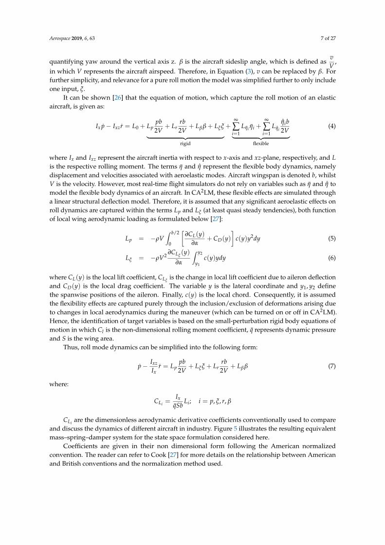
CLi are the dimensionless aerodynamic derivative coefficients conventionally used to compareand discuss the dynamics of different aircraft in industry. Figure 5 illustrates the resulting equivalentmass–spring–damper system for the state space formulation considered here.

Coefficients are given in their non dimensional form following the American normalizedconvention. The reader can refer to Cook [27] for more details on the relationship between Americanand British conventions and the normalization method used.

Aerospace 2019, 6, 63 8 of 27

Figure 5. Illustrations of equivalent mass–spring–damper roll model.

4.2. System Identification Process

Assuming the results obtained from the more complex physics based models used in CA2LMcan be compared to simplified and reduced order state space models given in Equation (8),a system identification procedure is used to identify the A and B matrices as a function of availablesimulation data.

x = Ax + Bu (8)

Multiple approaches can be used in system identification [28,29]. The first is the OrdinaryLeast Square method (OLS), which effectively tries to minimize the sum of squared differencesbetween the measurements or simulation results of the target model to identify (CA2LM in our case),and the idealized model (the state space equations of motion). Aircraft states x, x and input u areeffectively available to the algorithm to populate the A and B matrix based on a cost function definedaround the measurement equation. Appendix B highlights the formulation of the OLS method in moredetail. Given that all states are available in the simulation environment, the OLS does not requireany iterations and is an overall simpler formulation when compared to an alternative method suchas the output error method. More details on the identification theory can be found in References [28–30].

5. Aerodynamic Derivative Identification Results

5.1. Simulation Test Case

For this case study, a single mass case was considered at approximately 85% of Maximum Take-OffWeight (MTOW) with a Center of Gravity (CoG) at 25% of the mean aerodynamic chord. The wingtipplacement corresponded to 10% and 20% of wing semispan from the tip. For the AX-1 aircraft wingspan, this corresponds to 2.9 m and 5.8 m, respectively. A single hinge flare angle Λhinge = 17◦

was used herein. The aircraft was then flown in a finite set of symmetric folding configurations.Values ranging from Γwt = −20◦ (downward anhedral) to Γwt = +30◦ (upward dihedral) were used.Note that greater amplitudes would have led to critical local angles of attack beyond realistic stallconditions and limits of the model and were excluded from this investigation. The airframe was alsosimulated both as a rigid and flexible structure. As the first does not allow for the airframe to changeshape under folded or maneuver loads, the comparison highlighted the flexibility effects. A releasedwingtip configuration was also considered and was limited to flexible structure due to modelinglimitations discussed in previous chapters.

Keeping in mind the mass–spring–damper simplified model, the maneuver can be describedas follows [27]. First, as the aileron is deflected asymmetrically, rolling moment is introduced bythe overall differential lift from each wing directly highlighting aileron effectiveness Clξ . As the aircraftexperiences a controlled rolling moment, additional disturbing moment appears with angularacceleration p. During the roll, the wing undergoes a vertical velocity component (the intensity

Aerospace 2019, 6, 63 9 of 27

of which is a function of spanwise coordinate). This in turn, leads to a small increase in local flowincidence on the down-going starboard wing and vice versa on the up going wing. The differential liftgives the restoring rolling moment. The aircraft experiences both the disturbing and restoring rollingmoment until a steady roll rate is established. This restoring rolling moment is quantified by the rolldamping coefficient, Clp . Lastly, the aircraft roll angle introduces a small but perceivable sideslip angleas the aircraft is not constrained in lateral velocity. This sideslip angle coupled with wing dihedral alsoleads to differential lift generation, impacting aircraft roll through Clβ

.Introducing structural flexibility means that the structure adapts to the external aerodynamic loading

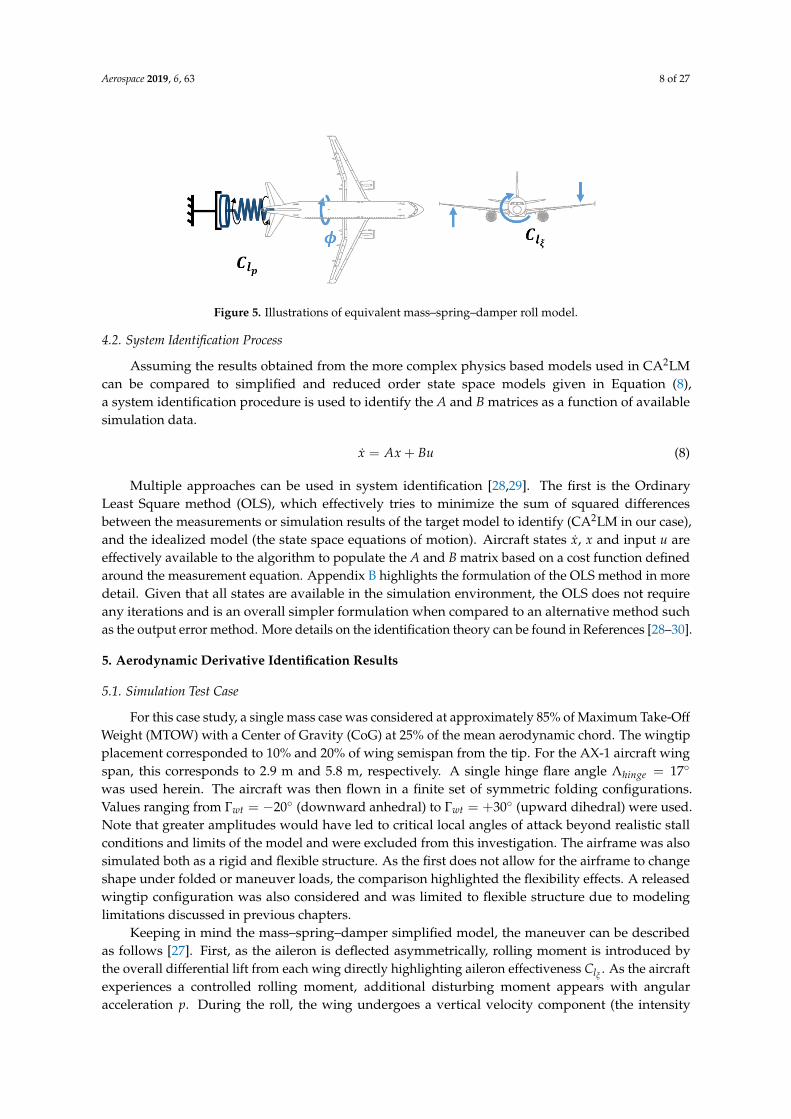
and undergoes deformation during perturbation (including aileron input). Different aerodynamic shapetherefore lead to changes in differential lift that generates the restoring rolling moment, thus affectingthe roll damping Clp as well as aileron effectiveness Clξ . Figure 6 illustrates, somewhat excessively,the typical shape changes between a folded and baseline wing in a flexible state.

Figure 6. Wing shape adaptation due to flexibility and wingtip folding.

A low amplitude aileron step was used to excite the aircraft roll motion, away from cruise trimmedcondition with a non-oscillatory lateral characteristic (additionally, low amplitude aileron doubletand 3-2-1-1 type inputs were used for comparison purposes, although not presented herein). Despitelow aileron deflections, steady state roll rate was achieved for the input deflection before large attitudechanges were reached. Small perturbations were introduced in the open-loop system, respectingthe assumptions required for the systems identification procedure whilst achieving maximum roll ratefor a given input which is important for aileron effectiveness identification.

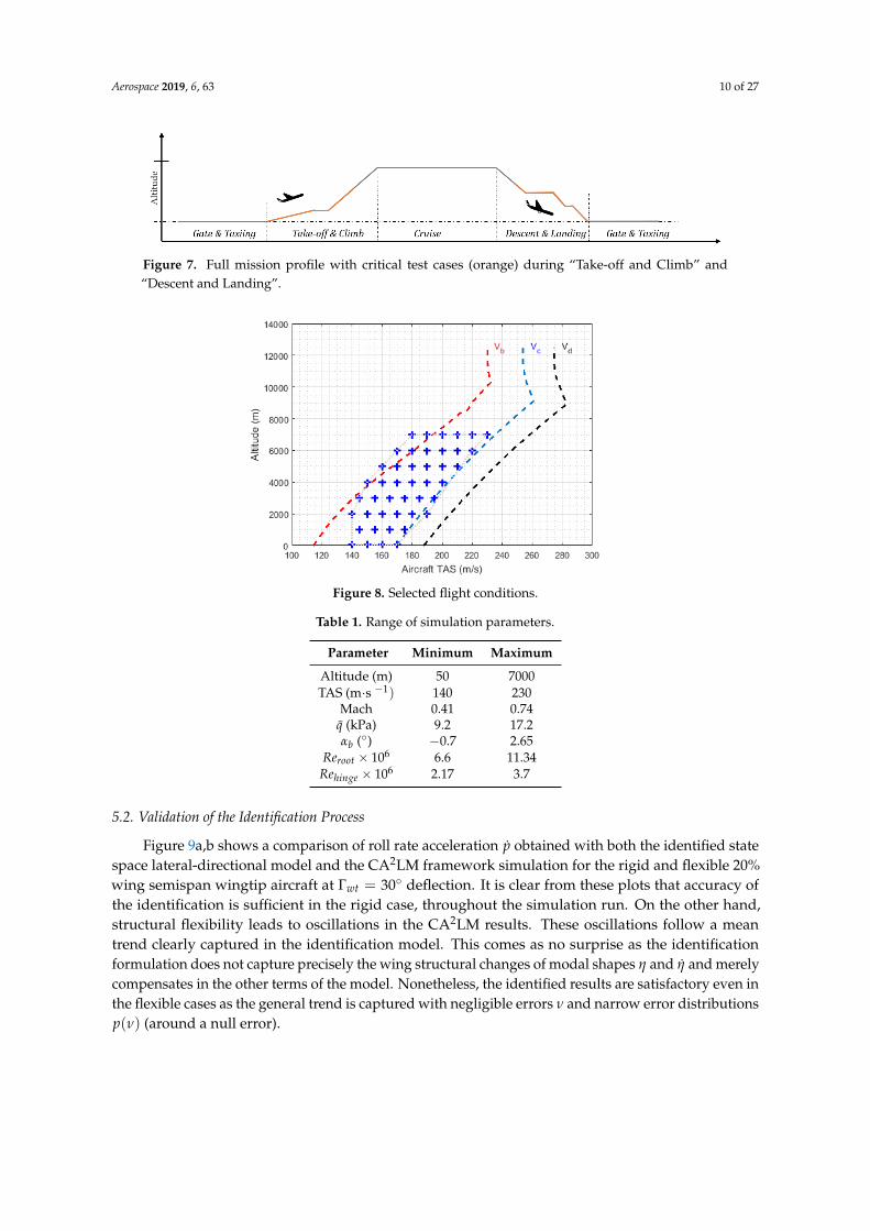
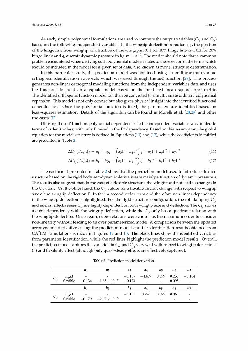
Flight conditions selected for this study correspond to the lower altitude and airspeeds of the AX-1design envelope so as to match dynamic pressure conditions comparable to “Take-off and Climb”and “Descent and Landing” conditions, as shown in Figure 7. Figure 8 highlights the 44 flight pointsselected throughout the flight envelope with ranges of dynamic pressures, altitude and airspeedsexperienced at these conditions being given in Table 1. Additionally, the full set of flight conditionsis given in Table A1 in Appendix C. The aircraft was considered in steady level flight, with a smallperturbation introduced to capture lateral dynamics. These conditions can be argued to be similar toloitering motion with large turn radius at constant altitude prior to landing. Climbing and descentflight paths were not considered due to framework trim set-up limitations.

At each of the flight conditions, the aircraft was trimmed in steady level flight in a baseline shapeusing conventional aircraft controls and no high lift devices (due to current modeling limitations).Trim is achieved after linearization of a reduced-order version of the model (for simplification reasons).An equilibrium (or trim) point was found for each conditions when the steady-state value for each ofthe state derivatives (with the exception of the aircraft position) was equal to zero (corresponding tosteady level flight). When applying symmetric folding input, a correction was applied to the elevatorto balance the pitching moment induced by the deflected wingtips and added to the trimmedelevator deflection.

Aerospace 2019, 6, 63 10 of 27

Figure 7. Full mission profile with critical test cases (orange) during “Take-off and Climb” and“Descent and Landing”.

Figure 8. Selected flight conditions.

Table 1. Range of simulation parameters.

Parameter Minimum Maximum

Altitude (m) 50 7000TAS (m·s −1) 140 230

Mach 0.41 0.74q (kPa) 9.2 17.2αb (◦) −0.7 2.65

Reroot × 106 6.6 11.34Rehinge × 106 2.17 3.7

5.2. Validation of the Identification Process

Figure 9a,b shows a comparison of roll rate acceleration p obtained with both the identified statespace lateral-directional model and the CA2LM framework simulation for the rigid and flexible 20%wing semispan wingtip aircraft at Γwt = 30◦ deflection. It is clear from these plots that accuracy ofthe identification is sufficient in the rigid case, throughout the simulation run. On the other hand,structural flexibility leads to oscillations in the CA2LM results. These oscillations follow a meantrend clearly captured in the identification model. This comes as no surprise as the identificationformulation does not capture precisely the wing structural changes of modal shapes η and η and merelycompensates in the other terms of the model. Nonetheless, the identified results are satisfactory even inthe flexible cases as the general trend is captured with negligible errors ν and narrow error distributionsp(ν) (around a null error).

Aerospace 2019, 6, 63 11 of 27

4 6 8 10 12-10

-5

0

510-3

Simulation ResultsIdentification Results

4 6 8 10 12-5

0

5

1010-4

-5 0 5 10

10-4

0

0.1

0.2

0.3

0.4

5 6 7 8 9 10 11 12-10

-5

0

510-4

Simulation ResultsIdentification Results

6 8 10 12-2

0

2

410-4

-2 0 2 4

10-4

0

0.05

0.1

0.15

(a) (b)

Figure 9. SID match for p of the AX-1 with 20% wingtip (aileron step input, TAS = 200 m·s−1

and h = 4575 m): (a) Γwt = 30◦ rigid; and (b) Γwt = 30◦ flexible.

5.3. Aerodynamic Derivative Shift Due to Wingtip Folding

As a result of small perturbation roll maneuver simulations at 44 flight conditions, multipleairframe flexibility and folding angles, an extensive database of Clp and Clξ values was generated.This allowed for trends in aerodynamic shifts to be identified. These results were also comparedto those of a similar aircraft configuration such as those obtained from flight test campaigns ofa Boeing B747 [31] and found to be adequately similar for both Clp and Clξ . On the other hand,due to the lack of directional coupling and the relatively low sideslip induced during the maneuver,the identification process led to less reliable and higher discrepancy in Clβ

estimates at a number offlight points and overall trends. This effectively led to these results not being included in the followingdiscussion (The authors are investigating alternative inputs and identification method for both Clβ

and Clr coefficients. Moreover, a coupled lateral-directional mathematical model would be requiredto adequately capture Clβ

, more relevant to coordinated turn (through a combination of rudderand aileron) than roll motion.).

Results presented herein are displayed as a function of both dynamic pressures q and angle ofattack αb, varying over the range of flight conditions. Smooth surface trends are obtained as a functionof these two parameters, selected for their relevance to pilots and flight dynamic analysis for furtherdevelopments. Re could also have been used (replacing q), although a secondary parameter suchas angle of attack would still have been required to better understand the trends captured herein.Figures 10 and 11 illustrate the trends in aerodynamic derivative changes due to flight conditions.Changes due to wingtip angle effectively lead to a shift of the entire surface as a function oflocal parameters.

It was found as expected that Clp values were not only dependent on the aerodynamic shapebut also on the flight conditions, as shown in Figure 10b for the larger wingtip variant of the testset-up, where Clp values for both rigid and flexible airframes in baseline (non folded) and foldedconfigurations are shown. These plots are based on the database generated in the scope of this work,an extract of which is included in Appendix E for the larger wingtip variant. Differences in the baselineClp values for both rigid and flexible body structure are obvious and come as a consequence ofthe change in aerodynamic shape. The latter is changed due to the steady aerodynamic loading as wellas the dynamic disturbance (roll rate). Introducing wingtip deflection also changes the aerodynamicloading, particularly tip-loading and overall aerodynamic lift and drag distributions, as shown inFigure 4. On the flexible structure, this forces the structure to adapt and bend, effectively forcingmore lift to be generated inboard of the hinge. As a consequence to this phenomenon, relatively small

Aerospace 2019, 6, 63 12 of 27

changes are observed on the Clp value in the flexible case when compared to the rigid structure. In fact,the same can be said for the Clξ value.

For the rigid aircraft, the Clp value varies up to 20% relative to the baseline (see Figure 10b orAppendix E) in the worst case for the rigid aircraft. Note that such a change in roll damping is expectedto be noticeable by the pilot if it is not corrected through the flight control system, though it shouldnot deteriorate handling qualities to undesirable standard. For the flexible aircraft, a much smallerchange of 0.7% is expected at the same flight and folding conditions, with an average of 2% expectedin upward folding. Note that the released wingtip cases lead to more noticeable and important Clp

changes of approximately 5–10%.

-0.6

-0.5

2

-0.4

-0.3

-0.2

1.5104 -1011 23

Released Wingtip (blue)

Baseline

Flexible Structure

Rigid StructureShift Limits

-0.6

-0.55

-0.5

-0.45

2

-0.4

-0.35

-0.3

-0.25

1.5

104 -101 123

Baseline

Shift Limits

Released Wingtip (blue)

Flexible Structure

Rigid Structure

(a) (b)

Figure 10. Clp variations against q and αb: (a) 2.9 m (10% wing semispan) wingtip device; and (b) 5.8 m(20% wing semispan) wingtip device.

0.02

0.03

0.04

-1

0.05

0.06

0.07

0.08

0.09

01 0.811.2

1042 1.41.61.83 2

Released Wingtip (blue)

Flexible Structure

Baseline

Rigid Structure

Shift Limits

0.02

0.03

0.04

-2

0.05

0.06

0.07

0.08

0.09

0 0.52 1

1041.54 2

Released Wingtip (blue)

Flexible Structure

Shift LimitsBaseline

Rigid Structure

(a) (b)

Figure 11. Clξvariations against q and αb: (a) 2.9 m (10% wing semispan) wingtip device; and (b) 5.8 m

(20% wing semispan) wingtip device.

A similar analysis can be made to explain the underlying reasons for the change in Clξ due toflexibility (and wingtip deflection). Changes in structural flexibility allows the aircraft to adapt tothe modified aerodynamic loading and partly counter the effect of the aileron input, thus loweringthe Clξ value compared to that of a rigid aircraft (Figure 11b for the larger wingtips). This phenomenonis not unheard of on very flexible wings where roll control inversion at high dynamic pressures havealready been discussed. Similarly, small changes to aileron effectiveness are introduced with wingtipdeflections. On the other hand, for the rigid body simulation set, the location of aileron and wingtiphinge line significantly impact the resulting Clξ value. In the 10% wing semispan wingtip, the outboard

Aerospace 2019, 6, 63 13 of 27

limit to the aileron is far enough from the hinge line (2.9 m) so that the wingtip deflection does notsignificantly impact the flow around the aileron. Aileron aerodynamics are not affected significantly.On the other hand, the 20% wing semispan wingtip size case introduces a hinge nearly overlappingwith the aileron outboard limit. Nonetheless, changes to aileron effectiveness remain relatively lowwith fold angle, with shifts ranging between 4% and −2% in both upward and downward deflections.On the other hand, the change in aerodynamic loading on the aileron during wingtip release leads toa significant change in Clξ value, with a maximum decrease of 12% relative to the baseline (Figure 11b)in aileron authority, linked by the authors to flapping wingtip effects. For the rigid case, a changebetween +5% and −8% is introduced.

A quick look at the results presented in Figures 10 and 11 can lead to the following statement:a greater change in roll dynamics is introduced when shifting from rigid to flexible airframe, thanwhen flying the aircraft with different fold angles throughout the flight envelope. Thus, it can bestated that switching from a rigid to a flexible aircraft would prove by far more challenging to a pilotthan the folding of the wingtips themselves.Additionally, it also shows that the wing flexibility greatlydampens or reduces the wingtip folding effects. In the case of a very rigid wing, the controlled foldingof the wingtips would have a greater impact on the aircraft response, as shown by the rigid simulationsgiven herein. These are very promising results for further development of the design as a lowerimpact of wingtip folding on the handling qualities of a flexible aircraft might lead to positive pilotperception of the system and relatively minor flight control law changes (at least for lateral control)can be expected.

Additionally, the authors believe that it is relevant to state that the released or loose wingtip stateappears in this study as most suitable for roll performances: with a decreased roll damping and onlyslight reduction in aileron authority, the authors believe that loose wingtips could be efficiently usedduring maneuvers to restore some roll performances lost by increasing the aircraft span in the caseof a HARW concept. Note that, with lower roll damping, the upward fold of the wingtip for a rigidaircraft gives a more suitable shape for roll maneuvers. With increasing wing flexibility, this effect candissipate, as seen herein. Note that aircraft range or climb performance are not considered and shouldalso be taken into account when considering suitable wingtip or winglet designs.

6. Prediction Model Derivation

The results from the identification process could be implemented directly in a flight simulatormodel or database to capture the impact of wingtip folding on the aircraft flight dynamics.However, this requires significant effort in terms of data transfer and implementation, for each aircraftand/or wingtip device. An alternative identified by the authors would be to implement a correctionor prediction model to account for the effect of folding wingtips on the aerodynamic derivativesas a function of simulation conditions. From previous results, it was found that the difference or shiftbetween baseline and folded configurations can be parametrized as a function of flight condition,wingtip size, and folding angle. Hence, such a prediction model could be built around the baseline rigidbody configuration for example and apply corrections to key aerodynamic derivatives as a function offlight conditions and wingtip parameters. The appropriate shift or ∆Cl could therefore be predictedwithout the needs for complex physics based models (as used in CA2LM) or extensive databases inthe aerodynamic derivative based simulators.

From findings presented in Section 5, such prediction models were hypothesized by the authorswith the following formulation:

CΓlp= CΓ=0

lp rigid

(1 + ∆Clp(Γ, ς, q)

)(9)

CΓlξ = CΓ=0

lξ rigid

(1 + ∆Clξ (Γ, ς, q)

)(10)

Aerospace 2019, 6, 63 14 of 27

As such, simple polynomial formulations are used to compute the output variables (Clp and Clη )based on the following independent variables: Γ, the wingtip deflection in radians; ς, the positionof the hinge line from wingtip as a fraction of the wingspan (0.1 for 10% hinge line and 0.2 for 20%hinge line); and q, aircraft dynamic pressure in kg·m−1·s−2. The reader should note that a commonproblem encountered when deriving such polynomial models relates to the selection of the terms whichshould be included in the model for a given set of data, also known as model structure determination.

In this particular study, the prediction model was obtained using a non-linear multivariateorthogonal identification approach, which was used through the mof function [28]. The processgenerates non-linear orthogonal modeling functions from the independent variables data and usesthe functions to build an adequate model based on the predicted mean square error metric.The identified orthogonal function model can then be converted to a multivariate ordinary polynomialexpansion. This model is not only concise but also gives physical insight into the identified functionaldependencies. Once the polynomial function is fixed, the parameters are identified based onleast-squares estimation. Details of the algorithm can be found in Morelli et al. [28,29] and otheruse cases [32].

Utilising the mof function, polynomial dependencies to the independent variables was limited toterms of order 3 or less, with only Γ raised to the Γ3 dependency. Based on this assumption, the globalequation for the model structure is defined in Equations (11) and (12), while the coefficients identifiedare presented in Table 2.

∆Clp(Γ, ς, q) = a1 + a2q +(

a3Γ + a4Γ2)

ς + a5Γ + a6Γ2 + a7Γ3 (11)

∆Clξ (Γ, ς, q) = b1 + b2q +(

b3Γ + b4Γ2)

ς + b5Γ + b6Γ2 + b7Γ3 (12)

The coefficient presented in Table 2 show that the prediction model used to introduce flexiblestructure based on the rigid body aerodynamic derivatives is mainly a function of dynamic pressure q.The results also suggest that, in the case of a flexible structure, the wingtip did not lead to changes inthe Clξ value. On the other hand, the Clp values for a flexible aircraft change with respect to wingtipsize ς and wingtip deflection Γ. In fact, a second-order term and therefore non-linear dependencyto the wingtip deflection is highlighted. For the rigid structure configuration, the roll damping Clp

and aileron effectiveness Clξ are highly dependent on both wingtip size and deflection. The Clp showsa cubic dependency with the wingtip deflection, while the Clξ only has a quadratic relation withthe wingtip deflection. Once again, cubic relations were chosen as the maximum order to considernon-linearity without leading to an over parameterized model. A comparison between the updatedaerodynamic derivatives using the prediction model and the identification results obtained fromCA2LM simulations is made in Figures 12 and 13. The black lines show the identified variablesfrom parameter identification, while the red lines highlight the prediction model results. Overall,the prediction model captures the variation in Clp and Clξ very well with respect to wingtip deflections(Γ) and flexibility effect (although only quasi-steady effects are effectively captured).

Table 2. Prediction model derivation.

a1 a2 a3 a4 a5 a6 a7

Clp

rigid - - −1.137 −1.677 0.079 0.250 −0.184flexible −0.134 −1.65× 10−5 −0.174 - - 0.095 -

b1 b2 b3 b4 b5 b6 b7

Clξ

rigid - - −1.133 0.296 0.087 0.065 -flexible −0.179 −2.67× 10−5 - - - - -

Aerospace 2019, 6, 63 15 of 27

(a) (b)

(c) (d)

Figure 12. Roll damping model (black: identified model, red: prediction model): (a) rigid model10% wingtip; (b) rigid model 20% wingtip; (c) flexible model 10% wingtip; and (d) flexible model20% wingtip.

(a) (b)

(c) (d)

Figure 13. Aileron effectiveness model (black: identified model, red: prediction model): (a) rigidmodel 10% wingtip; (b) rigid model 20% wingtip; (c) flexible model 10% wingtip; and (d) flexiblemodel 20% wingtip.

Aerospace 2019, 6, 63 16 of 27

To validate the prediction model further, a state space model based on Equation (7) and Clp

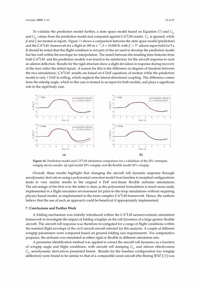
and Clξ values from the prediction model and compared against CA2LM results. Clr is ignored, whileβ and ξ are treated as inputs. Figure 14 shows a comparison between the state space model (prediction)and the CA2LM framework for a flight at 180 m·s−1, h = 10,000 ft, with ξ = 5◦ aileron input held for 5 s.It should be noted that this flight condition is not part of the set used to develop the prediction modelbut lies well within the envelope for interpolation. The match between the resulting time histories fromboth CA2LM and the prediction models was found to be satisfactory for the aircraft response to suchan aileron deflection. Results for the rigid structure show a slight deviation in response during recoveryof the turn (after the initial input). A reason for this is the difference in degrees of freedom betweenthe two simulations: CA2LM results are based on 6 DoF equations of motion while the predictionmodel is only 1 DoF in rolling, which neglects the lateral-directional coupling. The difference comesfrom the sideslip angle, which in this case is treated as an input for both models, and plays a significantrole in the rigid body case.

: 0 deg

: 30 deg : 30 deg

: 0 deg

(a) (b)

Figure 14. Prediction model and CA2LM simulation comparison for a validation of the 20% semispanwingtip device results: (a) rgid model 20% wingtip; and (b) flexible model 20% wingtip.

Overall, these results highlight that changing the aircraft roll dynamic response throughaerodynamic derivatives using a polynomial correction model from baseline to morphed configurationsleads to very similar results to the original 6 DoF non-linear flexible airframe simulations.The advantage of the first over the latter is clear, as the polynomial formulation is much more easilyimplemented in a flight simulator environment for pilot-in-the-loop simulations without requiringphysics based model, as implemented in the more complex CA2LM framework. Hence, the authorsbelieve that the use of such an approach could be beneficial if appropriately implemented.

7. Conclusions and Further Work

A folding mechanism was initially introduced within the CA2LM aeroservoelastic simulationframework to investigate the impact of folding wingtips on the roll dynamics of a large generic flexibleaircraft. The aircraft roll response was therefore investigated for a range of flight conditions withinthe nominal flight envelope of the civil aircraft aircraft selected for this analysis. A couple of differentwingtip parameters were compared based on ground folding size requirements. For comparativepurposes, the airframe was simulated as either rigid or flexible in different simulation sets.

A parameter identification method was applied to extract the aircraft roll dynamics as a functionof wingtip angle and flight conditions, with aircraft roll damping Clp and aileron effectivenessClξ aerodynamic derivatives presented herein. Results for the baseline configuration (no wingtipdeflection) were found to be similar to that of a comparable sized aircraft (the Boeing B747 [31] was

Aerospace 2019, 6, 63 17 of 27

used as a reference). The change in roll dynamics due to wingtip folding were less important whenthe airframe was given realistic flexibility, as the wing shape adapted to changes in aerodynamicloading. For the larger wingtip variant, both downward and upward deflections led to increases in Clp

amplitude of 4% and 2%, respectively, whilst a released wingtip led to a decrease in amplitude rangingbetween 5% and 10% when compared to the baseline at similar flight conditions. For Clξ , an averageincrease of 3% and 1.5% for downward and upward deflections, respectively, was introduced, whilstan average decrease of 10% emerged when releasing the wingtips. For the rigid structure, trendswere found to be different due to the lack of wing deflection changes and lift distribution differencesinduced by wingtip folding, with Clp modifications ranging from −5% (downward) to +12% (upward)and +5% and −7% for Clξ . Accurate numbers for these comparisons can be found in Appendix E,which includes an extract of the database generated in the scope of this work. The reader shouldnote that, in fact, the average difference between rigid and flexible aircraft derivatives at similar flightand wingtip conditions (approximately at 50% difference for Clp and 100% for Clξ scaled againstflexible data) were found to be greater throughout the range of tested positions and flight conditionsthan the shifts experienced throughout the test conditions. This result is not unexpected for largetubular body with swept wing configurations, and points to less drastic consequences of in-flightfolding wingtips on flight dynamics when flexibility is considered for swept wing aircraft. Thus, it canbe stated that switching from a rigid to a flexible aircraft would prove by far more challenging toa pilot than the folding of the wingtips themselves.

Overall, an aerodynamic derivative database was generated in order to be implemented toan engineering flight simulator, an extract of which is included in Appendix E. However, to avoida long and tedious manual implementation process (valid only for a given aircraft and wingtip system),a set of lateral aeroderivatives prediction models were developed instead. By taking into accountflexibility, wingtip deflection, wingtip size and flight conditions as input parameters, these models helppredict the dynamic response of an aircraft with in-flight wingtip folding by using a correction or ∆Clformulation to a conventional aeroderivative based flight dynamics model. As a result, two predictionmodels were developed for flexible and rigid configurations, applicable over a wide range of flightconditions and folding angles. Adequate correlation between the physics based folding model inCA2LM and the corrective prediction model applied to a linear state space formulation were found.These prediction models will then be implemented in a Cranfield Engineering Flight Simulatorfor pilot-in-the-loop investigations aimed at assessing the impact of wingtip folding on the aircrafthandling qualities.

As this paper focuses only on the roll dynamics of the aircraft, an extensive list of further workshould be considered. Firstly, a single mass case, center of gravity position and flare angle wereused herein. This must be extended further to validate the predictive model approach and allow formore reliable pilot-in-the-loop simulations for correct handling qualities investigations. Moreover,the quantification of the wingtip roll, yaw or pitch control derivative (similar to the aileron, rudderand elevator) could also be of interest. Additionally, the authors noted that directional and longitudinalmotion of the aircraft are also greatly influenced by wingtip folding and therefore require furtherinvestigations. The coupling of these dynamics in the system identification process applied toCA2LM is therefore a logical next step to capture the resulting coupled motion of the aircraft,making the identification of important additional lateral derivatives such as Clβ

and Clr more accurateand reliable. Finally, the identification of the aircraft aerodynamic derivatives in conditions different tosteady level flight (investigated herein) such as steady climb, descent or a banking turn (to mimic loiter,for instance) would also be interesting to capture the shifts in derivatives of interest, if significant, dueto other flight phase conditions.

Author Contributions: Conceptualization, G.D., S.Y. and M.L.; Methodology, G.D. and S.Y.; Software, G.D. andS.Y.; Validation, G.D. and S.Y.; Formal analysis, G.D. and S.Y.; Investigation, G.D. and S.Y.; Resources, G.D.; Datacuration, G.D.; Writing—original draft preparation, G.D.; Writing—review and editing, G.D..; Visualization, G.D.;Supervision, M.L.; Project administration, G.D. and M.L.

Aerospace 2019, 6, 63 18 of 27

Funding: This research received no external funding.

Acknowledgments: This work was supported and developed in collaboration with Airbus Group, Innovate UKand the Aerospace Technology Institute (UK ATI). The authors would also like to acknowledge the support ofthe Indonesia Endowment Fund for Education (Lembaga Pengelola Dana Pendidikan (LPDP)).

Conflicts of Interest: The authors declare no conflict of interest.

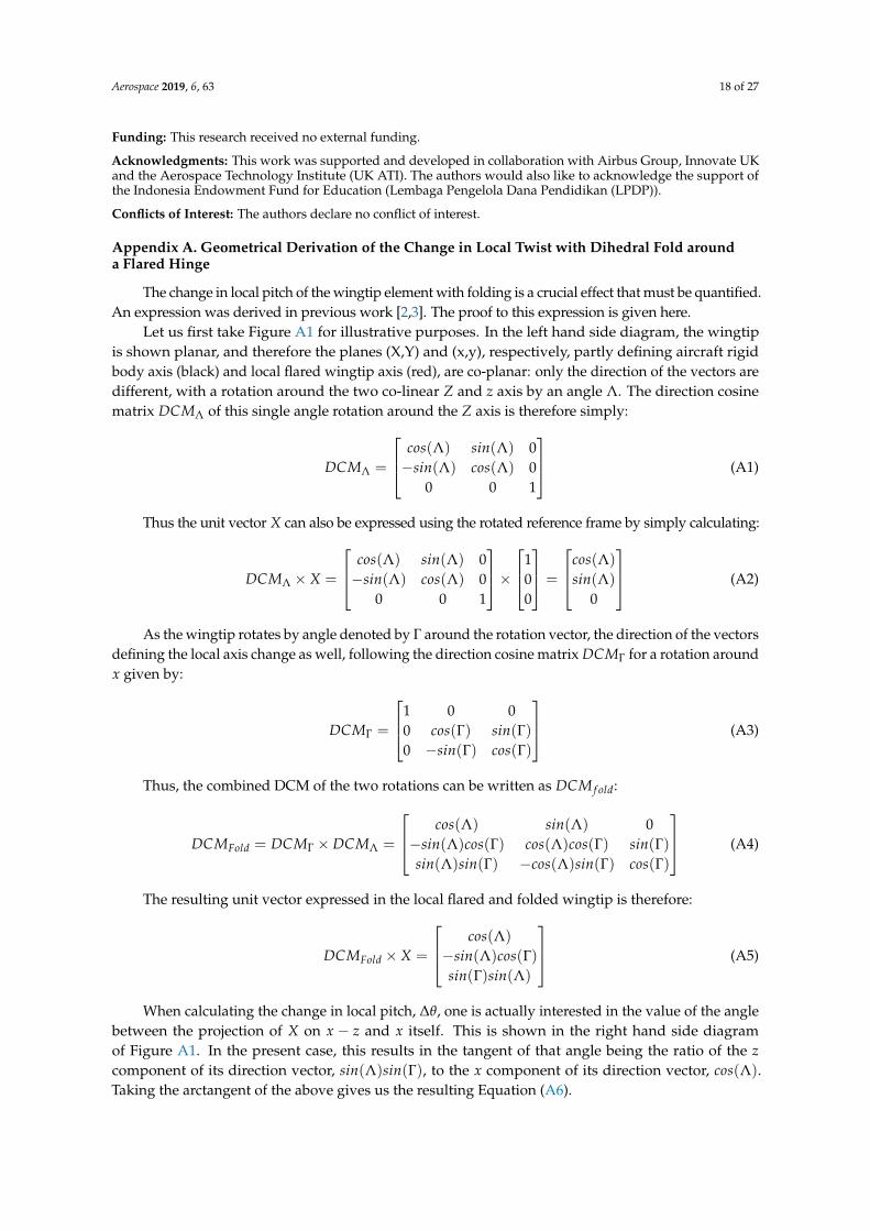
Appendix A. Geometrical Derivation of the Change in Local Twist with Dihedral Fold arounda Flared Hinge

The change in local pitch of the wingtip element with folding is a crucial effect that must be quantified.An expression was derived in previous work [2,3]. The proof to this expression is given here.

Let us first take Figure A1 for illustrative purposes. In the left hand side diagram, the wingtipis shown planar, and therefore the planes (X,Y) and (x,y), respectively, partly defining aircraft rigidbody axis (black) and local flared wingtip axis (red), are co-planar: only the direction of the vectors aredifferent, with a rotation around the two co-linear Z and z axis by an angle Λ. The direction cosinematrix DCMΛ of this single angle rotation around the Z axis is therefore simply:

DCMΛ =

cos(Λ) sin(Λ) 0−sin(Λ) cos(Λ) 0

0 0 1

(A1)

Thus the unit vector X can also be expressed using the rotated reference frame by simply calculating:

DCMΛ × X =

cos(Λ) sin(Λ) 0−sin(Λ) cos(Λ) 0

0 0 1

×1

00

=

cos(Λ)

sin(Λ)

0

(A2)

As the wingtip rotates by angle denoted by Γ around the rotation vector, the direction of the vectorsdefining the local axis change as well, following the direction cosine matrix DCMΓ for a rotation aroundx given by:

DCMΓ =

1 0 00 cos(Γ) sin(Γ)0 −sin(Γ) cos(Γ)

(A3)

Thus, the combined DCM of the two rotations can be written as DCM f old:

DCMFold = DCMΓ × DCMΛ =

cos(Λ) sin(Λ) 0−sin(Λ)cos(Γ) cos(Λ)cos(Γ) sin(Γ)sin(Λ)sin(Γ) −cos(Λ)sin(Γ) cos(Γ)

(A4)

The resulting unit vector expressed in the local flared and folded wingtip is therefore:

DCMFold × X =

cos(Λ)

−sin(Λ)cos(Γ)sin(Γ)sin(Λ)

(A5)

When calculating the change in local pitch, ∆θ, one is actually interested in the value of the anglebetween the projection of X on x − z and x itself. This is shown in the right hand side diagramof Figure A1. In the present case, this results in the tangent of that angle being the ratio of the zcomponent of its direction vector, sin(Λ)sin(Γ), to the x component of its direction vector, cos(Λ).Taking the arctangent of the above gives us the resulting Equation (A6).

Aerospace 2019, 6, 63 19 of 27

∆θ = tan−1 (tan (Λ)× sin (Γ)) (A6)

A validity check can be done through the verification of a number of boundary conditions.One can verify easily that Equation (A6) holds for:

• a fold angle of 0◦, as no pitch is introduced regardless of the flare of the hinge;• a fold angle of 90◦, as the resulting change in pitch is equal to the flare line, consistent with

a 90◦ rotation; and• a flare angle of 0◦ also leads to no pitch being introduced regardless of the fold angle.

Lastly, the trend in ∆θ over the entire spectrum of Λ and Γ was also verified for geometric consistency.

(a) (b)

Figure A1. Axis, reference frames and angles linked to wingtip change in pitch with fold:(a) top view—normal to (X,Y) plane; and (b) side view—normal to (x,z) plane.

Appendix B. OLS System Identification Method

Model parameters are identified using the ordinary least squares method, selected mainly dueto its simplicity. This method effectively tries to minimize the sum of squared differences betweenthe measurements and the idealized model. This approach requires the formulation of the followingmodel equation:

y = Xθ (A7)

and the measurement equation given as:

z = Xθ + ν (A8)

where z ∈ RN×1, θ ∈ Rnp×1, X ∈ RN×np and ν ∈ RN×1. The parameter vector θ is obtained byminimizing the following cost function:

J(θ) =12[z− Xθ] [z− Xθ]T (A9)

such thatθ = (XTX)−1Xz (A10)

In this case, the measurement equation is defined as:

z = p− Ixz

Ixr (A11)

while the regressor matrix for N number of data points, and the parameter vector defined as:

Aerospace 2019, 6, 63 20 of 27

X =

b

2Vp(1)

b2V

r(1) ∆β(1) δξ(1)...

......

...b

2Vp(N)

b2V

r(N) ∆β(N) δξ(N)

(A12)

θ =[

Lp Lr Lβ Lξ

]T(A13)

The observation equation is postulated as:

pm = p (A14)

in which the output-error method tries to minimize the difference between p from the CA2LM outputand pm.

Further details on the methods can be found in the relevant referenced documents [28,30].The estimation routine was based on the lesq function found in the SIDPAC library [28].

Appendix C. Simulation Trim Conditions

Table A1. Range of simulation parameters for the entire set of flight conditions considered.

FC Alt. (m) ν × 10−5 (m2·s−1) TAS (m·s−1) Mach q (Pa) αb (◦) Reroot × 106 Rehinge × 106

1 2000 1.715 140 0.42 9863 2.53 7.96 2.62 50 1.461 140 0.41 11,947 1.36 9.34 3.053 1000 1.581 145 0.43 11,686 1.45 8.94 2.924 3000 1.863 145 0.44 9557 2.70 7.59 2.485 2000 1.715 150 0.45 11,323 1.60 8.53 2.796 4000 2.028 150 0.46 9215 2.91 7.21 2.367 50 1.461 150 0.44 13,715 0.85 10.01 3.278 1000 1.581 155 0.46 13,354 0.68 9.56 3.129 3000 1.863 155 0.47 10,921 1.77 8.11 2.6510 2000 1.715 160 0.48 12,883 0.82 9.1 2.9711 4000 2.028 160 0.49 10,485 1.96 7.69 2.5112 5000 2.211 160 0.5 9422 2.65 7.06 2.313 50 1.461 160 0.47 15,605 −0.07 10.68 3.4914 1000 1.581 165 0.49 15,133 0.03 10.18 3.3215 3000 1.863 165 0.5 12,375 0.99 8.64 2.8216 2000 1.715 170 0.51 14,544 0.17 9.66 3.1617 4000 2.028 170 0.52 11,837 1.17 8.17 2.6718 5000 2.211 170 0.53 10,637 1.77 7.5 2.4519 50 1.461 170 0.5 17,616 −0.60 11.34 3.7120 6000 2.416 170 0.54 9533 2.43 6.86 2.2421 1000 1.581 175 0.52 17,022 −0.51 10.79 3.5222 3000 1.863 175 0.53 13,921 0.33 9.16 2.9923 2000 1.715 180 0.54 16,305 −0.37 10.23 3.3424 4000 2.028 180 0.55 13,270 0.50 8.65 2.8325 5000 2.211 180 0.56 11,925 1.03 7.94 2.5926 6000 2.416 180 0.57 10,687 1.62 7.26 2.3727 7000 2.646 180 0.58 9550 2.28 6.63 2.1728 3000 1.863 185 0.56 15,557 −0.23 9.68 3.1629 2000 1.715 190 0.57 18,167 −0.84 10.8 3.5330 4000 2.028 190 0.59 14,785 −0.07 9.13 2.9831 5000 2.211 190 0.59 13,287 0.39 8.38 2.7432 6000 2.416 190 0.6 11,908 0.91 7.67 2.533 7000 2.646 190 0.61 10,640 1.50 7 2.2934 3000 1.863 195 0.59 17,284 −0.71 10.21 3.3335 4000 2.028 200 0.62 16,383 −0.55 9.62 3.1436 5000 2.211 200 0.62 14,722 −0.15 8.82 2.8837 6000 2.416 200 0.63 13,194 0.31 8.07 2.6438 7000 2.646 200 0.64 11,790 0.84 7.37 2.4139 5000 2.211 210 0.66 16,231 −0.60 9.26 3.0240 6000 2.416 210 0.66 14,546 −0.18 8.47 2.7741 7000 2.646 210 0.67 12,998 0.29 7.74 2.5342 6000 2.416 220 0.7 15,965 −0.58 8.88 2.943 7000 2.646 220 0.7 14,266 −0.15 8.11 2.6544 7000 2.646 230 0.74 15,592 −0.50 8.48 2.77

Aerospace 2019, 6, 63 21 of 27

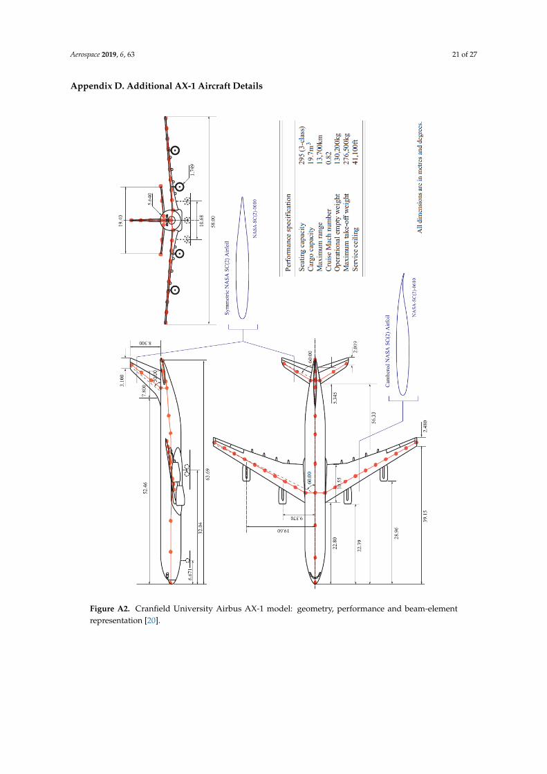
Appendix D. Additional AX-1 Aircraft Details

Figure A2. Cranfield University Airbus AX-1 model: geometry, performance and beam-elementrepresentation [20].

Aerospace 2019, 6, 63 22 of 27

Table A2. AX-1 wing, tail and fin geometric properties [16].

Component Dimension Value

Wing Area (m2) 363.1Aspect Ratio 9.260Taper Ratio 0.29Quarter Chord Sweep (◦) 30Mean Aerodynamic Chord (m) 7.279Semispan (m) 29

Tail Area (m2) 71.45Aspect Ratio 5.270Taper Ratio 0.3780Quarter Chord Sweep (◦) 30Mean Aerodynamic Chord (m) 3.932Semispan (m) 9.7

Fin Area (m2) 45.20Aspect Ratio 1.524Taper Ratio 0.3970Quarter Chord Sweep (◦) 40Mean Aerodynamic Chord (m) 5.788Semispan (m) 8.3

Appendix E. Additional AX-1 Aircraft Details

Table A3. Clp Identification results—20% wingtip rigid structure.

FC q (Pa) αb (◦) Γwt = −20◦ Γwt = 0◦ Γwt = 30◦

1 9863 2.53 −0.461 −5% ← −0.439 → −0.391 10.9%2 11,947 1.36 −0.46 −5% ← −0.438 → −0.389 11.2%3 11,686 1.45 −0.464 −5% ← −0.442 → −0.393 11.1%4 9557 2.70 −0.466 −5.2% ← −0.443 → −0.394 11.1%5 11,323 1.60 −0.469 −4.9% ← −0.447 → −0.397 11.2%6 9215 2.91 −0.47 −5.1% ← −0.447 → −0.398 11%7 13,715 0.85 −0.468 −4.7% ← −0.447 → −0.394 11.9%8 13,354 0.68 −0.472 −4.7% ← −0.451 → −0.398 11.8%9 10,921 1.77 −0.474 −5.1% ← −0.451 → −0.401 11.1%

10 12,883 0.82 −0.477 −4.8% ← −0.455 → −0.402 11.6%11 10,485 1.96 −0.478 −5.1% ← −0.455 → −0.405 11%12 9422 2.65 −0.479 −5.3% ← −0.455 → −0.405 11%13 15,605 −0.07 −0.477 −4.4% ← −0.457 → −0.397 13.1%14 15,133 0.03 −0.482 −4.6% ← −0.461 → −0.402 12.8%15 12,375 0.99 −0.482 −4.8% ← −0.46 → −0.407 11.5%16 14,544 0.17 −0.487 −4.7% ← −0.465 → −0.407 12.5%17 11,837 1.17 −0.487 −5% ← −0.464 → −0.411 11.4%18 10,637 1.77 −0.488 −5.2% ← −0.464 → −0.412 11.2%19 17,616 −0.60 −0.485 −3.4% ← −0.469 → −0.393 16.2%20 9533 2.43 −0.488 −5.2% ← −0.464 → −0.412 11.2%21 17,022 −0.51 −0.491 −3.8% ← −0.473 → −0.4 15.4%22 13,921 0.33 −0.492 −4.7% ← −0.47 → −0.412 12.3%23 16,305 −0.37 −0.497 −4.2% ← −0.477 → −0.408 14.5%24 13,270 0.50 −0.497 −4.6% ← −0.475 → −0.417 12.2%25 11,925 1.03 −0.498 −5.1% ← −0.474 → −0.419 11.6%26 10,687 1.62 −0.498 −5.1% ← −0.474 → −0.42 11.4%27 9550 2.28 −0.498 −5.1% ← −0.474 → −0.421 11.2%28 15,557 −0.23 −0.503 −4.6% ← −0.481 → −0.415 13.7%29 18,167 −0.84 −0.507 −3.5% ← −0.49 → −0.393 19.8%

Aerospace 2019, 6, 63 23 of 27

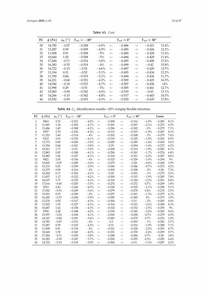
Table A3. Cont.

FC q (Pa) αb (◦) Γwt = −20◦ Γwt = 0◦ Γwt = 30◦

30 14,785 −0.07 −0.508 −4.5% ← −0.486 → −0.421 13.4%31 13,287 0.39 −0.509 −4.9% ← −0.485 → −0.426 12.2%32 11,908 0.91 −0.508 −5% ← −0.484 → −0.428 11.6%33 10,640 1.50 −0.508 −5% ← −0.484 → −0.429 11.4%34 17,284 −0.71 −0.514 −3.8% ← −0.495 → −0.408 17.6%35 16,383 −0.55 −0.519 −4% ← −0.499 → −0.42 15.8%36 14,722 −0.15 −0.52 −4.6% ← −0.497 → −0.429 13.7%37 13,194 0.31 −0.52 −5.1% ← −0.495 → −0.434 12.3%38 11,790 0.84 −0.519 −5.1% ← −0.494 → −0.436 11.7%39 16,231 −0.60 −0.531 −4.3% ← −0.509 → −0.425 16.5%40 14,546 −0.18 −0.531 −4.7% ← −0.507 → −0.436 14%41 12,998 0.29 −0.53 −5% ← −0.505 → −0.441 12.7%42 15,965 −0.58 −0.542 −4.4% ← −0.519 → −0.43 17.1%43 14,266 −0.15 −0.542 −4.8% ← −0.517 → −0.443 14.3%44 15,592 −0.50 −0.553 −4.5% ← −0.529 → −0.435 17.8%

Table A4. Clp Identification results—20% wingtip flexible structure.

FC q (Pa) αb (◦) Γwt = −20◦ Γwt = 0◦ Γwt = 30◦ Loose

1 9863 2.53 −0.321 −4.2% ← −0.308 → −0.314 −1.9% −0.283 8.1%2 11,947 1.36 −0.303 −4.1% ← −0.291 → −0.297 −2.1% −0.272 6.5%3 11,686 1.45 −0.308 −4.1% ← −0.296 → −0.302 −2% −0.275 7.1%4 9557 2.70 −0.326 −4.2% ← −0.313 → −0.319 −1.9% −0.287 8.3%5 11,323 1.60 −0.314 −4% ← −0.302 → −0.308 −2% −0.279 7.6%6 9215 2.91 −0.332 −4.1% ← −0.319 → −0.325 −1.9% −0.292 8.5%7 13,715 0.85 −0.296 −3.9% ← −0.285 → −0.289 −1.4% −0.269 5.6%8 13,354 0.68 −0.301 −3.8% ← −0.29 → −0.294 −1.4% −0.272 6.2%9 10,921 1.77 −0.32 −3.9% ← −0.308 → −0.314 −1.9% −0.283 8.1%

10 12,883 0.82 −0.308 −4.1% ← −0.296 → −0.301 −1.7% −0.276 6.8%11 10,485 1.96 −0.327 −4.1% ← −0.314 → −0.321 −2.2% −0.287 8.6%12 9422 2.65 −0.336 −4% ← −0.323 → −0.329 −1.9% −0.294 9%13 15,605 −0.07 −0.289 −3.6% ← −0.279 → −0.28 −0.4% −0.268 3.9%14 15,133 0.03 −0.295 −3.9% ← −0.284 → −0.286 −0.7% −0.272 4.2%15 12,375 0.99 −0.314 −4% ← −0.302 → −0.308 −2% −0.28 7.3%16 14,544 0.17 −0.302 −4.1% ← −0.29 → −0.293 −1% −0.275 5.2%17 11,837 1.17 −0.322 −4.2% ← −0.309 → −0.315 −1.9% −0.285 7.8%18 10,637 1.77 −0.332 −4.1% ← −0.319 → −0.326 −2.2% −0.291 8.8%19 17,616 −0.60 −0.283 −3.3% ← −0.274 → −0.272 0.7% −0.269 1.8%20 9533 2.43 −0.342 −4.3% ← −0.328 → −0.335 −2.1% −0.298 9.1%21 17,022 −0.51 −0.289 −3.6% ← −0.279 → −0.278 0.4% −0.272 2.5%22 13,921 0.33 −0.309 −4% ← −0.297 → −0.301 −1.3% −0.279 6.1%23 16,305 −0.37 −0.296 −3.9% ← −0.285 → −0.285 0% −0.275 3.5%24 13,270 0.50 −0.317 −4.3% ← −0.304 → −0.31 −2% −0.283 6.9%25 11,925 1.03 −0.327 −4.1% ← −0.314 → −0.321 −2.2% −0.288 8.3%26 10,687 1.62 −0.338 −4.3% ← −0.324 → −0.332 −2.5% −0.295 9%27 9550 2.28 −0.348 −4.2% ← −0.334 → −0.342 −2.4% −0.302 9.6%28 15,557 −0.23 −0.304 −4.1% ← −0.292 → −0.294 -0.7% −0.279 4.5%29 18,167 −0.84 −0.291 −3.6% ← −0.281 → −0.279 0.7% −0.276 1.8%30 14,785 −0.07 −0.312 −4% ← −0.3 → −0.303 −1% −0.283 5.7%31 13,287 0.39 −0.323 −4.2% ← −0.31 → −0.316 −1.9% −0.288 7.1%32 11,908 0.91 −0.334 −4% ← −0.321 → −0.328 −2.2% −0.293 8.7%33 10,640 1.50 −0.345 −4.2% ← −0.331 → −0.339 −2.4% −0.299 9.7%34 17,284 −0.71 −0.299 −3.8% ← −0.288 → −0.286 0.7% −0.28 2.8%35 16,383 −0.55 −0.307 −3.7% ← −0.296 → −0.295 0.3% −0.283 4.4%36 14,722 −0.15 −0.318 −3.9% ← −0.306 → −0.31 −1.3% −0.287 6.2%

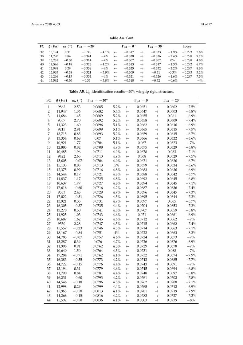
Aerospace 2019, 6, 63 24 of 27

Table A4. Cont.

FC q (Pa) αb (◦) Γwt = −20◦ Γwt = 0◦ Γwt = 30◦ Loose

37 13,194 0.31 −0.33 −4.1% ← −0.317 → −0.323 −1.9% −0.293 7.6%38 11,790 0.84 −0.341 −4% ← −0.328 → −0.336 −2.4% −0.298 9.1%39 16,231 −0.60 −0.314 −4% ← −0.302 → −0.302 0% −0.288 4.6%40 14,546 −0.18 −0.326 −4.2% ← −0.313 → −0.317 −1.3% −0.292 6.7%41 12,998 0.29 −0.338 −4% ← −0.325 → −0.332 −2.2% −0.297 8.6%42 15,965 −0.58 −0.321 −3.9% ← −0.309 → −0.31 -0.3% −0.293 5.2%43 14,266 −0.15 −0.334 −4% ← −0.321 → −0.326 −1.6% −0.297 7.5%44 15,592 −0.50 −0.33 −3.8% ← −0.318 → −0.32 −0.6% − −%

Table A5. ClξIdentification results—20% wingtip rigid structure.

FC q (Pa) αb (◦) Γwt = −20◦ Γwt = 0◦ Γwt = 20◦

1 9863 2.53 0.0685 5.2% ← 0.0651 → 0.0602 −7.5%2 11,947 1.36 0.0682 5.4% ← 0.0647 → 0.0603 −6.8%3 11,686 1.45 0.0689 5.2% ← 0.0655 → 0.061 −6.9%4 9557 2.70 0.0692 5.2% ← 0.0658 → 0.0609 −7.4%5 11,323 1.60 0.0696 5.1% ← 0.0662 → 0.0616 −6.9%6 9215 2.91 0.0699 5.1% ← 0.0665 → 0.0615 −7.5%7 13,715 0.85 0.0693 5.2% ← 0.0659 → 0.0615 −6.7%8 13,354 0.68 0.07 5.1% ← 0.0666 → 0.0622 −6.6%9 10,921 1.77 0.0704 5.1% ← 0.067 → 0.0623 −7%10 12,883 0.82 0.0708 4.9% ← 0.0675 → 0.0629 −6.8%11 10,485 1.96 0.0711 4.9% ← 0.0678 → 0.063 −7.1%12 9422 2.65 0.0713 4.9% ← 0.068 → 0.0629 −7.5%13 15,605 −0.07 0.0704 4.9% ← 0.0671 → 0.0626 −6.7%14 15,133 0.03 0.0713 5% ← 0.0679 → 0.0634 −6.6%15 12,375 0.99 0.0716 4.8% ← 0.0683 → 0.0636 −6.9%16 14,544 0.17 0.0721 4.8% ← 0.0688 → 0.0642 −6.7%17 11,837 1.17 0.0725 4.8% ← 0.0692 → 0.0645 −6.8%18 10,637 1.77 0.0727 4.8% ← 0.0694 → 0.0645 −7.1%19 17,616 −0.60 0.0716 4.2% ← 0.0687 → 0.0636 −7.4%20 9533 2.43 0.0729 4.7% ← 0.0696 → 0.0645 −7.3%21 17,022 −0.51 0.0726 4.5% ← 0.0695 → 0.0644 −7.3%22 13,921 0.33 0.0731 4.9% ← 0.0697 → 0.065 −6.7%23 16,305 −0.37 0.0735 4.4% ← 0.0704 → 0.0653 −7.2%24 13,270 0.50 0.0741 4.8% ← 0.0707 → 0.0659 −6.8%25 11,925 1.03 0.0743 4.6% ← 0.071 → 0.0661 −6.9%26 10,687 1.62 0.0745 4.6% ← 0.0712 → 0.0662 −7%27 9550 2.28 0.0747 4.5% ← 0.0715 → 0.0662 −7.4%28 15,557 −0.23 0.0746 4.5% ← 0.0714 → 0.0663 −7.1%29 18,167 −0.84 0.0751 4% ← 0.0722 → 0.0663 −8.2%30 14,785 −0.07 0.0757 4.6% ← 0.0724 → 0.0673 −7%31 13,287 0.39 0.076 4.7% ← 0.0726 → 0.0676 −6.9%32 11,908 0.91 0.0762 4.5% ← 0.0729 → 0.0678 −7%33 10,640 1.50 0.0764 4.5% ← 0.0731 → 0.068 −7%34 17,284 −0.71 0.0762 4.1% ← 0.0732 → 0.0674 −7.9%35 16,383 −0.55 0.0773 4.2% ← 0.0742 → 0.0685 −7.7%36 14,722 −0.15 0.0776 4.4% ← 0.0743 → 0.0691 −7%37 13,194 0.31 0.0779 4.6% ← 0.0745 → 0.0694 −6.8%38 11,790 0.84 0.0781 4.4% ← 0.0748 → 0.0697 −6.8%39 16,231 −0.60 0.0793 4.2% ← 0.0761 → 0.0702 −7.8%40 14,546 −0.18 0.0796 4.5% ← 0.0762 → 0.0708 −7.1%41 12,998 0.29 0.0799 4.4% ← 0.0765 → 0.0712 −6.9%42 15,965 −0.58 0.0813 4.1% ← 0.0781 → 0.0719 −7.9%43 14,266 −0.15 0.0816 4.2% ← 0.0783 → 0.0727 −7.2%44 15,592 −0.50 0.0836 4.1% ← 0.0803 → 0.0739 −8%

Aerospace 2019, 6, 63 25 of 27

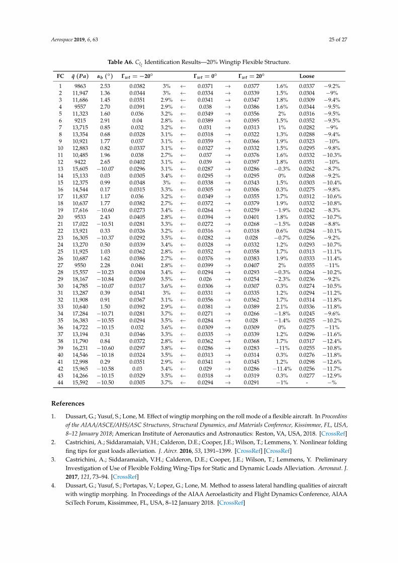
Table A6. ClξIdentification Results—20% Wingtip Flexible Structure.

FC q (Pa) αb (◦) Γwt = −20◦ Γwt = 0◦ Γwt = 20◦ Loose

1 9863 2.53 0.0382 3% ← 0.0371 → 0.0377 1.6% 0.0337 −9.2%2 11,947 1.36 0.0344 3% ← 0.0334 → 0.0339 1.5% 0.0304 −9%3 11,686 1.45 0.0351 2.9% ← 0.0341 → 0.0347 1.8% 0.0309 −9.4%4 9557 2.70 0.0391 2.9% ← 0.038 → 0.0386 1.6% 0.0344 −9.5%5 11,323 1.60 0.036 3.2% ← 0.0349 → 0.0356 2% 0.0316 −9.5%6 9215 2.91 0.04 2.8% ← 0.0389 → 0.0395 1.5% 0.0352 −9.5%7 13,715 0.85 0.032 3.2% ← 0.031 → 0.0313 1% 0.0282 −9%8 13,354 0.68 0.0328 3.1% ← 0.0318 → 0.0322 1.3% 0.0288 −9.4%9 10,921 1.77 0.037 3.1% ← 0.0359 → 0.0366 1.9% 0.0323 −10%10 12,883 0.82 0.0337 3.1% ← 0.0327 → 0.0332 1.5% 0.0295 −9.8%11 10,485 1.96 0.038 2.7% ← 0.037 → 0.0376 1.6% 0.0332 −10.3%12 9422 2.65 0.0402 3.1% ← 0.039 → 0.0397 1.8% 0.0351 −10%13 15,605 −10.07 0.0296 3.1% ← 0.0287 → 0.0286 −0.3% 0.0262 −8.7%14 15,133 0.03 0.0305 3.4% ← 0.0295 → 0.0295 0% 0.0268 −9.2%15 12,375 0.99 0.0348 3% ← 0.0338 → 0.0343 1.5% 0.0303 −10.4%16 14,544 0.17 0.0315 3.3% ← 0.0305 → 0.0306 0.3% 0.0275 −9.8%17 11,837 1.17 0.036 3.2% ← 0.0349 → 0.0355 1.7% 0.0312 −10.6%18 10,637 1.77 0.0382 2.7% ← 0.0372 → 0.0379 1.9% 0.0332 −10.8%19 17,616 −10.60 0.0273 3.4% ← 0.0264 → 0.0259 −1.9% 0.0242 −8.3%20 9533 2.43 0.0405 2.8% ← 0.0394 → 0.0401 1.8% 0.0352 −10.7%21 17,022 −10.51 0.0281 3.3% ← 0.0272 → 0.0268 −1.5% 0.0248 −8.8%22 13,921 0.33 0.0326 3.2% ← 0.0316 → 0.0318 0.6% 0.0284 −10.1%23 16,305 −10.37 0.0292 3.5% ← 0.0282 → 0.028 −0.7% 0.0256 −9.2%24 13,270 0.50 0.0339 3.4% ← 0.0328 → 0.0332 1.2% 0.0293 −10.7%25 11,925 1.03 0.0362 2.8% ← 0.0352 → 0.0358 1.7% 0.0313 −11.1%26 10,687 1.62 0.0386 2.7% ← 0.0376 → 0.0383 1.9% 0.0333 −11.4%27 9550 2.28 0.041 2.8% ← 0.0399 → 0.0407 2% 0.0355 −11%28 15,557 −10.23 0.0304 3.4% ← 0.0294 → 0.0293 −0.3% 0.0264 −10.2%29 18,167 −10.84 0.0269 3.5% ← 0.026 → 0.0254 −2.3% 0.0236 −9.2%30 14,785 −10.07 0.0317 3.6% ← 0.0306 → 0.0307 0.3% 0.0274 −10.5%31 13,287 0.39 0.0341 3% ← 0.0331 → 0.0335 1.2% 0.0294 −11.2%32 11,908 0.91 0.0367 3.1% ← 0.0356 → 0.0362 1.7% 0.0314 −11.8%33 10,640 1.50 0.0392 2.9% ← 0.0381 → 0.0389 2.1% 0.0336 −11.8%34 17,284 −10.71 0.0281 3.7% ← 0.0271 → 0.0266 −1.8% 0.0245 −9.6%35 16,383 −10.55 0.0294 3.5% ← 0.0284 → 0.028 −1.4% 0.0255 −10.2%36 14,722 −10.15 0.032 3.6% ← 0.0309 → 0.0309 0% 0.0275 −11%37 13,194 0.31 0.0346 3.3% ← 0.0335 → 0.0339 1.2% 0.0296 −11.6%38 11,790 0.84 0.0372 2.8% ← 0.0362 → 0.0368 1.7% 0.0317 −12.4%39 16,231 −10.60 0.0297 3.8% ← 0.0286 → 0.0283 −11% 0.0255 −10.8%40 14,546 −10.18 0.0324 3.5% ← 0.0313 → 0.0314 0.3% 0.0276 −11.8%41 12,998 0.29 0.0351 2.9% ← 0.0341 → 0.0345 1.2% 0.0298 −12.6%42 15,965 −10.58 0.03 3.4% ← 0.029 → 0.0286 −11.4% 0.0256 −11.7%43 14,266 −10.15 0.0329 3.5% ← 0.0318 → 0.0319 0.3% 0.0277 −12.9%44 15,592 −10.50 0.0305 3.7% ← 0.0294 → 0.0291 −1% - −%

References

1. Dussart, G.; Yusuf, S.; Lone, M. Effect of wingtip morphing on the roll mode of a flexible aircraft. In Proceedinsof the AIAA/ASCE/AHS/ASC Structures, Structural Dynamics, and Materials Conference, Kissimmee, FL, USA,8–12 January 2018; American Institute of Aeronautics and Astronautics: Reston, VA, USA, 2018. [CrossRef]

2. Castrichini, A.; Siddaramaiah, V.H.; Calderon, D.E.; Cooper, J.E.; Wilson, T.; Lemmens, Y. Nonlinear foldingfing tips for gust loads alleviation. J. Aircr. 2016, 53, 1391–1399. [CrossRef] [CrossRef]

3. Castrichini, A.; Siddaramaiah, V.H.; Calderon, D.E.; Cooper, J.E.; Wilson, T.; Lemmens, Y. PreliminaryInvestigation of Use of Flexible Folding Wing-Tips for Static and Dynamic Loads Alleviation. Aeronaut. J.2017, 121, 73–94. [CrossRef]

4. Dussart, G.; Yusuf, S.; Portapas, V.; Lopez, G.; Lone, M. Method to assess lateral handling qualities of aircraftwith wingtip morphing. In Proceedings of the AIAA Aeroelasticity and Flight Dynamics Conference, AIAASciTech Forum, Kissimmee, FL, USA, 8–12 January 2018. [CrossRef]

Aerospace 2019, 6, 63 26 of 27

5. Allerton, D. Principles of Flight Simulation; John Wiley & Sons: Chichester, West Sussex, UK, 2009; p. 471,ISBN 0470682191.

6. Lockheed Martin Official Website. 2014. Available online: https://www.lockheedmartin.com/us/news/features/2014/5-unique-f35c-carrier-variant-features.html (accessed on 1 December 2017).

7. Bradley, M.K.; Droney, C.K. Subsonic Ultra Green Aircraft Research: Phase II: N + 4 AdvancedConcept Development; Technical Report NASA/CR-2012-217556; NASA: Hanover, MD, USA, 2012.

8. Hayes, D.; Lone, M.; Whidborne, J.; Coetzee, E. Evaluating the rationale for folding wing tips comparing theexergy and Breguet approaches. In Proceedings of the 55th AIAA Aerospace Sciences Meeting, Grapevine,TX, USA, 9–13 January 2017. [CrossRef]

9. Kamlet, M.; Gibbs, Y. NASA Tests New Alloy to Fold Wings in Flight; NASA: Edwards, CA, USA, 2018.10. Pace, S. North American XB-70 Valkyrie; Aero Series #30; Aero Publishers: New York, NY, USA, 1990; p. 98,

ISBN 0830686207.11. Jenkins, D.R.; Landis, T. North American XB-70A Valkyrie; Specialty Press: Thurgoona, Australia, 2002; p. 104,

ISBN 1580070566.12. Dussart, G.; Lone, M.; O’Rourke, C.; Wilson, T. In-flight folding wingtip system: Inspiration from the

XB-70 Valkyrie. Morphing Wings II. In Proceeding of the AIAA SciTech Forum, San Diego, CA, USA, 7–11January 2019.

13. Bourdin, P.; Gatto, A.; Friswell, M.I. Aircraft control via variable cant-angle winglets. J. Aircr. 2008,45, 414–423. [CrossRef] [CrossRef]

14. Mills, J.; Ajaj, R. Flight dynamics and control using folding wingtips: An experimental study. Aerospace2017, 4, 19. [CrossRef] [CrossRef]

15. Kandath, H.; Pushpangathan, J.; Bera, T.; Dhall, S.; Bhat, M.S. Modeling and closed loop flight testing of afixed wing micro air vehicle. Micromachines 2018, 9, 111. [CrossRef] [CrossRef] [PubMed]

16. Andrews, S.P. Modelling and Simulation of Flexible Aircraft: Handling Qualities with Active Load Control.Ph.D. Thesis, Cranfield University, School of Engineering, Bedford, UK, 2011.

17. Dussart, G.; Portapas, V.; Pontillo, A.; Lone, M. Flight dynamic modelling and simulation of large flexibleaircraft. In Flight Physics—Models, Techniques and Technologies; InTech: London, UK, 2018. [CrossRef]

18. Leishman, J.G.; Nguyen, K.Q. State-space representation of unsteady airfoil behaviour. AIAA J. 1990,28, 836–844. [CrossRef]

19. Leishman, J.G.; Beddoes, T.S. A generalised model for airfoil unsteady aerodynamic behaviour anddynamic stall using the indicial method. In Proceedings of the 42nd Annual forum, Washington, DC,USA, 2–4 June 1986.

20. Lone, M. Pilot Modelling for Airframe Loads Analysis. Ph.D. Thesis, Cranfield University, School ofAerospace, Transport and Manufacturing, Bedford, UK, 2013.

21. Lone, M.; Dussart, G. Impact of spanwise non-uniform discrete gusts on civil aircraft loads. Aeronaut. J.2019, 123, 93–120. [CrossRef]

22. Portapas, V.; Cooke, A.K.; Lone, M. Modelling framework for flight dynamics of flexible aircraft. Aviation2016, 20, 173–182. [CrossRef]

23. Carrizales, M.; Dussart, G.; Portapas, V.; Pontillo, A.; Lone, M. Comparison of reduced order aerodynamicmodels and RANS simulations for whole aircraft aerodynamics. In Proceeding of the AIAA AtmosphericFlight Mechanics Conference, Kissimmee, FL, USA, 8–12 January 2018. [CrossRef]

24. Lone, M.; Cooke, A. Pilot-model-in-the-loop simulation environment to study large aircraft dynamics.J. Aerosp. Eng. 2012, 227, 555–568. [CrossRef] [CrossRef]

25. Lone, M.; Lai, C.K.; Cooke, A.; Whidborne, J. Framework for flight loads analysis of trajectory-basedmanoeuvres with pilot models. J. Aircr. 2014, 51, 637–650. [CrossRef] [CrossRef]

26. Waszak, M.R.; Buttril, C.S.; Schmidt, D.K. Modeling and Model Simplification of Aeroelastic Vehicles: An Overview;Technical Report; National Aeronautics and Space Administration: Hampton, VA, USA, 1992.

27. Cook, M.V. Flight Dynamics Principles: A Linear Systems Approach to Aircraft Stability and Control, 3rd ed.;Elsevier Aerospace Engineering Series; Butterworth-Heinemann: Oxford, UK, 2013; ISBN 978-0-08-098242-7.

28. Klein, V.F.; Morelli, E.A. Aircraft System Identification. Theory and Practice; AIAA Education Series; AIAA:Reston, VA, USA, 2006; ISBN 9781563478321.

Aerospace 2019, 6, 63 27 of 27

29. Morelli, E.A.; DeLoach, R. Wind tunnel database development using modern experiment design andmultivariate orthogonal functions. In Proceedings of the 41st Aerospace Sciences Meeting and Exhibit, Reno,NV, USA, 6–9 January 2003. [CrossRef]

30. Jategaonkar, R.V. Flight Vehicle System Identification: A Time Domain Methodology; AIAA: Reston, VA, USA, 2006;p. 534. [CrossRef]

31. Heffley, R.K.; Jewell, W.F. Aircraft Handling Qualities Data; Technical Report; NASA: Washington, DC,USA, 1972.

32. Yusuf, S.; Chavez, O.; Lone, M. Application of multivariate orthogonal functions to identify aircraft fluttermodes. In Proceedings of the AIAA Atmospheric Flight Mechanics Conference, AIAA SciTech Forum,Grapevine, TX, USA, 9–13 January 2017. [CrossRef]

c© 2019 by the authors. Licensee MDPI, Basel, Switzerland. This article is an open accessarticle distributed under the terms and conditions of the Creative Commons Attribution(CC BY) license (http://creativecommons.org/licenses/by/4.0/).