Identification and control of the Rotary InvertedPendulumArnolds, M.B.

Published: 01/01/2003

Document VersionPublisher’s PDF, also known as Version of Record (includes final page, issue and volume numbers)

Please check the document version of this publication:

• A submitted manuscript is the author's version of the article upon submission and before peer-review. There can be important differencesbetween the submitted version and the official published version of record. People interested in the research are advised to contact theauthor for the final version of the publication, or visit the DOI to the publisher's website.• The final author version and the galley proof are versions of the publication after peer review.• The final published version features the final layout of the paper including the volume, issue and page numbers.

Link to publication

General rightsCopyright and moral rights for the publications made accessible in the public portal are retained by the authors and/or other copyright ownersand it is a condition of accessing publications that users recognise and abide by the legal requirements associated with these rights.

• Users may download and print one copy of any publication from the public portal for the purpose of private study or research. • You may not further distribute the material or use it for any profit-making activity or commercial gain • You may freely distribute the URL identifying the publication in the public portal ?

Take down policyIf you believe that this document breaches copyright please contact us providing details, and we will remove access to the work immediatelyand investigate your claim.

Download date: 16. Jul. 2018

Identification and control ofthe Rotary Inverted

Pendulurn

M.B.Arnolds

DCT Report no: 2003.100october 2003

TU/ e Traineeship Reportoctober 2003

Supervisors:Prof. LMareelsUniversity of Melbourne, AustraliaProf. dr. H.NijmeijerTechnische Universiteit Eindhoven

Eindhoven University of TechnologyDepartment of Mechanical EngineeringDivision Dynamical Systems DesignDynamics Control Technology Group

In cooperation with:University of Melbourne, AustraliaDepartment of Electrical and Electronic EngineeringCooperative Research Centre for Sensor Signal and Infor­mation Processing (CSSIP)

Abstract

Research on under-actuated systems becomes more and more popular nowa­days. If it is possible to control an under-actuated system, it is possible todesign a light construction (i.e. the amount of motors will reduce) which willlead to less inertia. A simple example of an under-actuated system is the Ro­tary Inverted Pendulum setup (or often called the Furuta Pendulum), which isa system with two degrees of freedom and only one actuator. In this report, theidentification and the control of this system are discussed in order to be ableto balance the pendulum in upright position.

Contents

Abstract

1 Introduction

2 The inverted pendulum model

2.1 Setup introduction ...

2.2 Derivation of the model

3 Calibration

3.1 Servo potentiometer

3.2 Optical encoder.

3.3 Motor dead-zone

4 ParalTIeter Estimation

4.1 Estimators. . . . . .

4.2 Directly measured parameters

4.3 Parameters concerning the pendulum only

4.3.1 Off-line simulations.

4.3.2 Experiments ....

4.4 Parameters concerning total setup

4.4.1 Off-line simulations .

4.4.2 Experiments

4.5 Summary ......

5 Control of the pendulum

5.1 Swing up controller.

5.2 Switching Strategy .

5.3 Balancing controller

5.3.1 Linearized model

5.3.2 Discrete time model

5.3.3 Incremental discrete time model

ii

1

2

2

2

7

7

8

9

11

12

13

14

14

15

17

18

19

23

25

25

27

28

28

29

30

CONTENTS

5.3.4 Control law . . . . ..

5.3.5 Controller for setup 2

5.4 Summary . . . . . . . . . . .

6 Conclusions and Recommendations

6.1 Conclusions ....

6.2 Recommendations

A Calibration Results

B Numerical Results of PE experiments

C Design of an EKF for the pendulum rod

D Design of an EKF for the total system

D.1 2 states and 4 parameters

D.2 2 states and 3 parameters

E Linearisation of the non-linear model

III

31

36

38

39

39

39

41

43

46

49

49

54

55

Chapter 1

Introduction

The vertical positioning of the inverted pendulum requires a continuous correctionmechanism to stay upright because this set-point is unstable in an open-loop configu­ration. This can be compared to a rocket launch. The rocket boosters have to be firedin a controlled matter in order to keep the rocket upright.

The goal of this project is to perform this balancing act with a rotary inverted pendulumsetup. The description of the setup will be given in chapter 2. Before designinga balancing controller several steps have to be taken first. Deriving a mathematicalmodel of the inverted pendulum setup is the first step in the design process (chapter 2).It is important to create such a model for the system to be able to describe the responseof the actual system as closely as possible. Lagrange's equations of motion will be usedfor this. The model gives the relationships among all the variables involved except forinherent model uncertainties like flexibilities and slack. With this model it is possibleto estimate the unknown parameters of the system. Before the parameter estimationcan be performed it is necessary to calibrate the encoders on the setup (chapter 3). Forthe estimation of the parameters, an Extended Kalman Filter (EKF) will be designedand applied (chapter 4). At the end of the project, once the all parameters of thesystem are known, the design of a hybride controller will be discussed (chapter 5).This controller will consist of three parts. The combination of these three parts willmake the setup able to swing-up and balance the pendulum in upright position whichis the main goal of the project.

In between it is necessary to learn how to write a program in C++, because the KriInverted Pendulum pp-300 setup that is located at the University of Melbourne hasits own processor "board which can only read C++. This learning process will not bediscussed in this report.

The practical part of this traineeship and writing the main part of this report is per­formed at the University of Melbourne at the department of Electrical and ElectronicEngineering, under the supervision of prof. 1. Mareels. The finishing of the report isperformed back in the Netherlands at the TU/ e, under the supervision of prof. dr. H.Nijmeijer.

1

Chapter 2

The inverted pendulum model

2.1 Setup introduction

A schematic picture of the so-called Furuta pendulum setup is shown in Figure 2.1.The setup has two degrees of freedom: the rotation of the arm and the rotation of the

z

}-,x

Figure 2.1: Schematic drawing of the setup

pendulum rod. It is a so called under-actuated system so only one of the rotations isforced where the other one has a free response to it. The rotation of the arm, a, isactuated by putting a torque on the motor. The position of a is measu~ed with anoptical encoder. The motion, (3, of the pendulum rod is a free rotation depending onthe actuated arm rotation. It is measured with a servo potentiometer. The calibrationand resolution of the encoder and potentiometer will be discussed later on.

2.2 Derivation of the model

A model of the pendulum can be found in [Berg03]. After checking the model someerrors were discovered so the model will be derived again in this report. The derivationstarts with the Lagrange equations of motion. Because of the two degrees of freedompresent in the system, as indicated in Figure 2.1, a set of generalized coordinates is:

(2.1)

2

CHAPTER 2. THE INVERTED PENDULUM MODEL 3

Here a is the position of the actuated rotating arm and (3 is the position of the un­actuated pendulum rod. See Figure 2.1. The downward position of the pendulum isconsidered as (3 = O.

To determine the kinetic energy of the system, the position of the considered mass ml(located at the center of mass of the pendulum rod, see section 4.2) must be expressedin the generalized coordinates mentioned in (2.1).

(

10 cos a - h sin a sin (3 )I:ml = 10 sin a + h cos a sin (3 .

-h cos (3(2.2)

Here 10 and h represents the lengths as shown in Figure 2.1. The velocity of the massml is then:

-&10 sin a - &h cos a sin (3 - 13h sin a cos (3 )&10 cos a - &h sin a sin (3 + 13h cos a cos (3 .

13h sin (3

(2.3)

The total kinetic energy of the systems can be written as:

(2.4)

Jzo and J z1 represents the moments of inertia for respectively the actuated arm andthe pendulum rod. When (2.3) and (2.4) are combined the total kinetic energy become:

The potential energy of the system in terms of the generalized coordinates is given by:

v = -m19hcos(3. (2.6)

In order to bring viscous damping into account, virtual work has to be implemented.First take the work from the virtual displacement OflT = [oa, 0]:

oW = -[Co&]oa + TmOa = Qaoa.

Next OflT = [0,0(3] will be applied:

These equations lead to the nonconservative generalized forces

The Lagrange's equations of motion are then:

~ 8L _ 8L = Qnedt 8q 8q ,

with L = T - V.This can also be written as:

(2.7)

(2.8)

(2.9)

(2.10)

(2.11)

CHAPTER 2. THE INVERTED PENDULUM MODEL 4

Resulting in the equations of motion of the system:

]­

](2.12)

Which in a more standard form can be written as:

(2.13)

[ ~ ] +

[ ~ ] +

[ m1gl~ sin (3 ] = [ TO ]

[Jzo + m1lg + m1li sin2 (3 m1lohcos(3]

mllohcos(3 JZ1 + m1li

Co + m1li /3 sin (3 cos (3 m1lia sin (3 cos (3 - mlloh/3 sin (3 ]-m1lia sin (3 cos (3 C1

Now the equation of motions are defined, the next step is to define T m since the inputgiven to the setup is not a real torque. The input given is a real number (either positiveor negative) with no units. The input will be called u. The scheme for the motor isshown in Figure 2.2. So it is necessary to determine the relationship between u and

Ra La

+U

PWM +Amplifier

Ku

Figure 2.2: Electrical model of the motor

Tm . The voltage Vm is a result from conversing and amplifying the input u with a fac­tor K u , which will be called the gain of the PWM (Pulse Width Modulation) amplifier.

Vm = Kuu.

From Kirchhoff's voltage law it is easy to see that:

dIaVm = laRa + Ladi + E b,

(2.14)

(2.15)

with:I a the armature current,R a armature coil resistance,La armature coil inductance,E b motor's back EMF.

The motor's back EMF, Eb, is proportional to the rate of change of magnetic flux andhence proportional to the angular velocity of the motor:

(2.16)

CHAPTER 2. THE INVERTED PENDULUM MODEL 5

For a constant field current, the torque T exerted by the motor is proportional to thearmature current. This leads to:

(2.17)

When assuming that the coil inductance had a negligible influence, the torque exertedby the motor becomes:

(2.18)

Finally the dry friction that is present in the setup has to be implemented. The frictionin the rotation of the pendulum rod ((3) is considered to be totally modelled by theviscous damping term in the model. However, the dry friction present in the rotation ofthe actuated arm (0:) is not yet modelled. This is a little bit more complicated becausethis is so-called Coulomb friction. Coulomb friction is difficult to model but often it ismodelled as:

Ff = K f . sign(a). (2.19)

This means that it is discontinuous if the velocity is equal to zero. See Figure 2.3.

Figure 2.3: K f . sign(a)

This discontinuity is certainly not desirable because of the use of certain integrationmethods later on. Because ofthis an approximation ofthe sign-function will be used tomodel the dry friction of the actuated arm. A proper approximation will be a sigmoidfunction like:

2o-(a) == 1 - --;2:-;-k:-.­

e a + 1(2.20)

When k is chosen large enough (Le. k = 15) this function will provide a good approxi­mation of the sign-function (see Figure 2.4).The disadvantage of this approximation is that the stick-phase in the usually presentstick- and slip-phase will not be modelled here.

So now the dry friction can be written as:

(2.21 )

CHAPTER 2. THE INVERTED PENDULUM MODEL 6

0.5

.S /

.6

.4

.2

0

.2

.4

.6

.S )-

-0

Figure 2.4: Sigmoid function (2.20) with k=15

The two types of friction can be combined so the total friction model for the armrotation is obtained.

Ftotal = Kj(J'(a) + Coa

This is graphical presented in Figure 2.5.

(2.22)

/ / Co/

/

/

>~/a

Figure 2.5: Combined friction (2.22)

After combining (2.13), (2.18) and (2.20), the total equations of motion for the invertedpendulum setup are obtained.

[Jzo + m1l6 + m1lr sin2

j3 m1lohCOSj3]m1lohcosj3 J Z1 + m1lr

Co + K;{b + m1zI/3sinj3cosj3 m1zIasinj3cosj3 - m1loh/3 sin j3 ]-m1lrasinj3cosj3 C1

[Kj' (J'(a) ] _ [

m19h sinj3 -

(2.23)

Chapter 3

Calibration

The angular measurement data recorded from the system, raw data, are defined incounts. These counts are a result of the output of the optical encoder and servopotentiometer (See Section 2.1). So to obtain the right input signals for the parameterestimation this raw data has to be converted to useful data, radians in stead of counts.To do so a calibration of both setups has to be made. This calibration is already donein [Berg03] but since one of the setups (setup 2) is replaced this will be done again,but will not be discussed so extensively. For this the same experiments will be usedwhile these have proved to work properly.

3.1 Servo potentiometer

There will be 4 kind of experiments to determine the relation between the amount ofcounts and the real angle position (in degrees) of the servo potentiometer.

• From 0° to 180° in counterclockwise direction,

• From 0° to 180° in clockwise direction,

• From 0° to 270° in ee and back, 0° to 90° in e and back,

• From 0° to 270° in ee, 270° to 180° in ee, 180° to 270° in e.

Every movement within a program is repeated 5 times. The results are tabled inappendix A, tables A.1 to A.5.

After processing the data of the experiments one can see they are, for both setups,almost the same as already obtained in [Berg03]. There may be a difference in themeasurements of 1 or 2 counts. The conclusions however will not be the same. For anextended calculation reference is made to [Berg03].

Experiment 3 for setup 1 shows that the counts for f3 = 90° and f3 = 270° are almostat the perfect 256 counts. This involves an equally distributed range over the total360°, meaning that each count stands for 90°/256 = 0.351°. Experiments 1 and 2both show a mean value of 507 counts in stead of the expected 512 counts. Thisdifference of 5 . 0.351° = 1.7° from the upright position is quite reasonable for nakedeye positioning. Looking at experiment 4 it seems the potentiometer has a blind zone.To be more precise; a direction dependent blind zone.

As can be seen from Figure 3.1 the blind zone is direction dependent. Travelling inclockwise direction, the counts leave the normal count cycle at 717 (= 251.6°) and

7

CHAPTER 3. CALIBRATION 8

enters it at -306 (= 252.6°). This difference of 1 degree will be neglected. However,travelling in counterclockwise direction, the counts exit the normal count cycle at theexpected -306 counts but do not enter again at the also expected 717 but at 640. Thismeans a blind zone of 27° in CC direction. The cross-over point (point where the valuejumps 1023 counts up or down) is located at -107.4°.

For setup 2, experiment 3 shows a mean value for (3 = 90° and (3 = 270° of about 275counts. From experiments 1 and 2 the average amount of counts at 0° and 180° is 544counts. This means that the distribution over 90° is 90°/274 = 0.33°/count. As wellas setup 1 setup 2 has a blind zone but this one is not direction dependent as can beseen from the results of experiment 4. This blind zone starts (looking at the clockwisedirection) at 701 . 0.33 = 231° and ends at -322 . 0.33 = -106° = 253°. So a blindzone of 22° is present.

Setup I Setup 2

/1060

" Blind zone

o "

!--­-----~

""'... I

" lClockwise '---! ~-----

Figure 3.1: Blind zones of servo potentiometers. For setup 1: direction dependent.For setup 2: non-direction dependent. (mention that the drawn angels are a little bitexaggerated)

These blind zones in the measurements will not disturb the estimation of the parametersbecause the excitation of the pendulum can be limited to avoid entering this blind zones.Of course, during closed loop control it is not possible to avoid these blind zones andthese have to be taken into account.

3.2 Optical encoder

For the calibration of the optical encoder the same method is used as with the servopotentiometer: manual movement of the arm while the encoder records the signals. Anextended calibration is already done in [Berg03] so here the same experiments will bedone just to compare the results.

As said, the arm will be moved manually. To avoid the reset boundary of the opticalencoder, first the arm will make 4 rotations in clockwise direction continued with amovement of 8 rotations in counterclockwise direction and after that 4 rotations inclockwise direction again. With the 8 rotations the maximum number of rotations isreached. This experiment is done three times. Afterwards, the directions of movementwill be inverted and the experiment will be done another three times.

The experimental results seem to be in agreement with the results of [Berg03]. That isfor setup 1 an average of 52330 counts per 8 rotations which is 18.17 counts per degree.

CHAPTER 3. CALIBRATION

Start Counts per 8 rotationsDirection Setup 1 Setup 2

C exp 1 52254 52512C exp 2 52242 52616C exp 3 52170 52566

CC exp 1 52548 52502CC exp 2 52288 52542CC exp 3 52482 52294

Mean 52330 52505

Table 3.1: Results of calibration Optical Encoder

9

For setup 2 it is an average of 52505 counts per 8 rotations which is 18.23 counts perdegree.

3.3 Motor dead-zone

Because of the static friction in the arm suspension and the motor the driver input uthat is put on the motor has to reach a certain value before the motor will start to move.This will be called the dead-zone of the motor. These boundaries have to be knownbefore doing experiments for the parameter estimation. Two kind of experiments havebeen performed to measure the transition from static to dynamic friction (the momentwhen the arm will start to move). The first type (A) will increase the input step bystep (1 unit per step) every 2 seconds. The second one (B) will do the same but willjump back to zero between the two steps. This is done because this would happen incontrolling the system. The experiments are performed in positive as well as negativedirection. The average results are presented in Table 3.3. All the results are presentedin Table A.5.

Determining the value for u for which the arm starts to move, a safety zone is takeninto account, Figure 3.2. This safety zone is determined by looking at the motion ofa. One can see the motion already starts at the beginning of the safety zone but to besure the motor has totally overcome the static friction the value of u will be determineda short period later.

- Positive input Negative inputType A TypeB Type A Type B

Setup 1 45.4 45.6 -43.8 -44.6Setup 2 28.4 36.4 -30.4 -38.4

Table 3.2: Average results of motor dead-zone experiment

The motor dead-zone is determined. So the effective value for u should be > 45 forsetup 1 and > 40 for setup 2. The fact that the dead-zone for setup 1 is bigger as forsetup 2 can be confirmed with the fact that it takes more power to rotate the arm ofsetup 1 manually then the arm of setup 2. This means there is more static frictionpresent and so the dead-zone will be bigger. The difference between the two different

CHAPTER 3. CALIBRATION

•

..•

Figure 3.2: ~Iethod to determine the value u for the dead-zolle

10

experimcllts is small. Controlling the system (balancing the pendulum in upright posi­lion) will be done by correcting the position of the arm with ~shock wisc~ pulses. So,especially for setup 2, the difference that is present will be very useful.

The dead-zolle is schematic presented as:

•

Figure 3.3: Schematic presentation of dead-zollc of the motor

Chapter 4

Parameter Estimation

For the design of a good controller for the system all parameters which are involved inthe system equation must be known. Since this isn't the case, the unknoWn parametershave to be derived or estimated.

The estimation of the parameters can be divided in three groups:

• parameters that can be measured directly,

• parameters that can be estimated with an experiment considering only the pen­dulum,

• parameters that can only be estimated with an experiment considering the totalsetup.

In table 4.1 the three groups and their parameters are presented:

Directly measured m1, lo, hExperiment involving only pendulum Jz1 , C1

Experiment involving total setup Jzo, Co, K t , K b, K u , Ra , K f

Table 4.1: 3 groups and their parameters

It shows 12 parameters that have to be estimated. This can be reduced to 10 parameterssince the 4 parameters from the motor only arise in the model in combination witheach other (KtKb and K,K,,).

R a R a

11

CHAPTER 4. PARAMETER ESTIMATION

4.1 Estimators

12

An optimal estimation algorithm is an algorithm which processes measurements toderive an estimation (with minimum error) of a parameter by using the knowledgeof cthe system and the measurements, assumptions about statistics of system noiseand measurement errors and information of initial conditions. The advantage of suchan estimation algorithm is that it uses all the previous measurement data and theknowledge of the system.

One can distinguish 3 different types of estimators:

e filtering

• smoothing

• prediction

Filtering is when the moment of estimation is the same as the moment of the lastmeasurement. Smoothing is when the moment of estimation is somewhere in the timespan of the measurement and it is prediction if the moment of estimation will be afterthe moment of the last measurement. For the next part of this report filtering will beused because on every moment an estimation will be made, a measurement is known.

The Least Square Method (LSQM) could be used. This is a discrete time method. Itis a numerical optimization routine which selects the best combination of parametersin such a way that it minimizes the fit error. The fit error is defined to be a scalar costfunction so that fit errors at all data points are taken into account in determining thebest value for the parameters.

i = datapoints (4.1)

This way, the best fitted parameters to the system equations will be obtained.

Another filter is a Kalman filter. The advantage of a Kalman filter is that it uses allthe previous knowledge and measurement data to update its estimation. Because theproblem is a non-linear problem, an Extended Kalman Filter (EKF) will be designed.The equations for a continuous EKF are [Gelb74]:

i = [(~(t), t) + K((£ -l1(x, t)) (4.2)

P = F(x(t), t)P(t) + P(t)FT(x(t), t) + Q(t)

- P(t)HT(x(t), t)R- 1(t)H(x(t), t)P(t) (4.3)

K = P(t)HT(x(t), t)R-1 (t) (4.4)

The vectors f(~(t), t), l1.(x, t) and the matrices F(x(t), t), H(x(t), t), P(t), R(t) aredefined in Appendix C. Also initial conditions for P (Po) and ~ (~o) are necessary.These initial conditions are required for solving the Kalman equations (4.2 - 4.4).

Every moment a new value for i will be calculated by using the old estimated value ofi and the measurement at that moment. After that a new P matrix can be calculated.By integration of i and P the values for ~ and P are obtained which are used tocalculate a new Kalman gain K. The Kalman gain takes care of updating the system.With the new value of K a new i can be calculated again. .

The EKF is preferred to use above the Least Square Method to estimate the parametersof this system. The measurement will be in discrete time and the EKF is continuoustime but this will not cause any problems since the use of the integration method DDE45

in Matlab will overcome this difference.

CHAPTER 4. PARAMETER ESTIMATION 13

4.2 Directly measured parameters

As stated before the lengths lo, h and the mass ml can be directly measured andcalculated.

IDweight

1 total

1weight

,,,,,,,

: _..<--I-"ro""d~_,,

I I----I i---

Ipivot

11:_..<----"---__ I

I II II II II I

Figure 4.1: Pendulum rod parameters

Figure 4.1 shows the pendulum rod with its masses. With this information hand ml

can be obtained. Assuming that the mass is equally distributed along the pendulumrod,

ltotalmrod = mrod = 20.48 gr

ltotal + lpivot(4.5)

so,ml = mrod + mweight = 27.6 gr

Using the law of moment the effective length h can be obtained.

(4.6)

(4.7)

The results:

I Parameter I Result Comment

la 154.7 mm 11easured directly

h 145 mm Calculated

ml 27.6 gram Calculated

Table 4.2: Results of group 1

CHAPTER 4. PARAMETER ESTIMATION

4.3 Parameters concerning the pendulum only

14

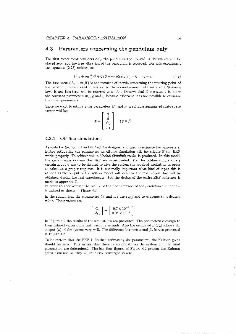
The first experiment considers only the pendulum rod. 0: and its derivatives will bestated zero and the free vibration of the pendulum is recorded. For this experimentthe equation (2.23) reduces to:

(4.8)

The first term (Jzl + milt) is the moment of inertia concerning the rotating point ofthe pendulum constructed in relation to the normal moment of inertia with Steiner'slaw. Hence this term will be referred to as Jr1 . Observe that it is essential to knowthe constant parameters ml, 9 and h because otherwise it is not possible to estimatethe other parameters.

Since we want to estimate the parameters 0 1 and J1 a suitable augmented state-spacevector will be:

;r.=

4.3.1 Off-line simulations

;y = (3.

As stated in Section 4.1 an EKF will be designed and used to estimate the parameters.Before estimating the parameters an off-line simulation will investigate if the EKFworks properly. To achieve this a Matlab Simulink model is produced. In this modelthe system equation and the EKF are implemented. For this off-line simulations acertain input u has to be defined to give the system the required excitation in orderto calculate a proper response. It is not really important what kind of input this isas long as the output of the system model will look like the real output that will beobtained during the real experiments. For the design of the entire EKF reference ismade to appendix C.In order to approximate the reality of the free vibration of the pendulum the input uis defined as shown in Figure 4.2:

In the simulations the parameters 0 1 and Jrl are supposed to converge to a definedvalue. These values are:

[0 1 ] [0.7 X 10-

3]

Jrl = 0.08 X 10-3

In Figure 4.2 the results of the simulations are presented. The parameters converge totheir defined values quite fast, within 2 seconds. Also the estimated (3 ((3e) follows theoutput (z) of the system very well. The difference between z and (3e is also presentedin Figure 4.2.

To be certain that the EKF is finished estimating the parameters, the Kalman gainsshould be zero. This means that there is no update on the system and the finalparameters are determined. The last four figures of Figure 4.2 present the Kalmangains. One can see they all are nicely converged to zero.

CHAPTER 4. PARA.~·lE'TER ESTIMATION 15

"""'U """'" y• 10~ y.',

0.' 0

0

OS 0

, '000 ,0 .. " 0 .. " 0 .. ", '''''' • 10" C, .10· J"... "'" • ..

"'" 1000 (I. • •'000 " '( - • -

00 • ,

'000 '000 • '00 .. " 0 .. " 0 .. " .. "", .,0' K, .. ".... 3 ..... , 0 0... , ~., .,

'" \ 0 1\ ~., .,

0 ., ~3 ·30 .. " 0

nme1Psecl " 0 .. " 0 .. "lime (sec) lime (sec) b.... (sec)

Figurc 4.2: Results of thc simulation for pendulum

4.3.2 Experiments

Now the Kalman filter is working propcrly some experimcnts call be donc. In thcsimulation part an input u was set on thc systcm to obtain a response. To obtain afrC() response during thc cxperimcnts a \'cry short and quick input will be set on thesystem so the pendulum will get an excitation. The first concern is to get familiar withprogramming the system. This turns out to be quite tricky. But after SC\'cral cxper·iments useful data is recorded sllccessfully. With this data, the parameter estimationis performed off-line by loading it into lhe workspace of Matillb and usc it as the inputof the EKF.

The signal recorded for {J is very smooth and almOllt free of noise. Because of this thedata will not be filtered. This will save the data from losing magnitudc.

For cach setup 5 cxperimcnts wcre done. All the numerical results are shown in TableB.I of Appendix B. The graphs in Figure 4.3 and Figure 4,4 summarize the results.It is clear that the Kalman filter has coll\'crged as wcll as thc parametcrs. The crrorbetween thc mcasured {J ({J... ) and the estimated {J ({Jc) is around 2 % for both setups,which is acceptable.

CHAPTER 4. PARA1...IETER ESTIMATION 16

meuur.cl p.. p•. p.,",.

111111111111111111110.'"

11i1\V-'~J'0 0

o • 11111111111111111110

0..~II'I '

0 "20 010 "

,.'. , .. _10 J C ,_ 10' '0,

",

,.1111111111111111111 : IIIIIIIIIIIIIIMIWI •

0 ,. •0.' 11111111I11111111110 .jlllIlIlJnIl " ,,

" 00 "

,. 0 ",.

",. 0 "

,." _ 10' K., .. ,

"'" " " •"" " 02

i1•. 0

"" • 0

11 •0 0 02

"" • " 20 1000 ",. 0 "

,. 0 " ",.

Figure 4.3: Results of parameters estimation C, and J, for Setup 1

ITIllllSU red p... Pm - p., 0."

" i~""j~WN~WI00'

0

IIIII1 II ,I0

" 00',

2(f04 00 " ",., ,.. _ 10" C _ 10'" J, ,..~ •

0.'

Ijl.III~III~II~~!Ii.! IINIIIIM :If0 •0 ,\.

11111 11 I ",.

",,. "0 ,. 00 ,. 000 " " " "

,." • 10· ., ., '."'" • 0' •

"" " ~\llh', 0,.. 0

II'0 •0 .,.,.. ., ., ."0 "

,. 0 ",. 0 "

,. 0 ",.

Figure 4.4: Results of parameters estimation C, and J1 for Setup 2

CHAPTER 4. PARAMETER ESTIMATION 17

After these experiments we successfully obtained the values for the parameters 0 1 andJr1 .

I Parameter I Setup 1 Setup 2 I

~][~]-[

C1 [kgm2 js] 0.1 x 10 -;:) 0.12 x 10 3

±0.013 x 10-3 ±0.0025 x 10-3

Jr1 [kgm2] 0.79 x 10 3 0.77 x 10 3

±0.0009 x 10-3 ±0.0002 x 10-3

Table 4.3: Results of parameters estimation Pendulum rod

4.4 Parameters concerning total setup

After the estimation of the parameters of the pendulum only, the parameters of theentire system have to be estimated. For this the total model equation has to be used.After rewriting equation (2.23) we obtain:

m 1 li;3 sin,B cos,B-m1lia sin,B cos,B

-Jzoo

(4.9)

Only the first equation will be used as the system equation. But to simplify the model,i3 will be extracted from the second equation and substituted in the first one. It is thesame as taking the inverse of the first matrix and multiply all the other matrices withthis inverse. ,B will be defined as an input of the system (with ;3 as its time-derivative),so Ci only depends on a, ,B and ;3.

From the second equation we obtain:

i3 = - m1lOh cos,B Ci + m1li sin,B cos,B a2 _ 0 1 ;3 ~ m1gh sin,B.Jr1 Jr1 Jrl Jr1

(4.10)

Substituting equation (4.10) into the first equation of (4.9) and extracting Ci the systemequation for the entire system is obtained:

(4.11)

CHAPTER 4. PARAMETER ESTIMATION

with:

(-(Co + KR~b) - 2mlli/3sin 13 cos 13)11 = 21212 2 fJ '

J + l2+ l2' 2 13 m) 0 ) coszO ml 0 ml 1 SIn - J

r)

m,i lozi sin {3 cos2 (3

12 == Jr1

2 2 2 2 ,

J + l2 + l2' 213 m)IOI) cos fJzO ml 0 ml 1 SIn - J

r)

Kf13= 21212 2fJ'

J + l2 + l2' 2 13 m) 0 , coszO ml 0 mi 1 SIn - J

r1

C,m,loZ,!3cosfJ + =i9lolisinfJcosfJ + l lj3'2 . 13Jrl Jrl ml 0 1 sm

14 = 21212 2 fJ 'J + l2+ l2' 2 13 =) Q 1 cos

zO ml 0 ml 1 SIn - Jr

)

KtKu

f ~5 = 21212 2 fJ .

J + l2 + l2' 2 13 m, Q ) coszO ml 0 ml 1 SIn - Jrl

18

So now a vector ;£ can be specified for only 2 states and 4 parameters instead of 4states and 4 parameters. Since it is impossible to distinguish the contribution of Coand KR~b separately, these will be estimated together as one parameter.

;£=

These equations are used for the design of the EKF (appendix D) and implemented inSimulink.

4.4.1 Off-line simulations

The approach will be the same as used for the estimation of the parameters for thependulum rod only (section 4.3). This time an input u as well as 13 have to be defined.Again it does not really matter what kind of input this is, but since we will use a step­function (the reason for this will be a point of discussion in section 4.4.2) for ex in thereal model it will also be used in the simulation. For 13 a simple sine-response is taken.This may not be a really good approximation of the reality but for the simulationsit will turn out to be good enough. In the Simulink model Ci is calculated and twiceintegrated to obtain ex. To obtain the needed /3, the time-derivative of 13 is taken. Thismay cause some problems for the real experiments because ofthe noise but if a low-passfilter is used, these problems are probably solved.

The input u that is used for the simulation is shown in Figure 4.5 Again the parametersare supposed to converge to certain defined values.

r Kftu 1 r 3.5 x 10-3 1

l Jzo J l0.9 X 10-3 J

Co + KR~b = 8.8 x 10-:K f 1.0 x 10-

The results of the simulations are presented in Figure 4.5. To check if the EKF has

CIlAPTcn 4. PARAMETER ESTIAlATION 19

X10. 3 P"" x 10" p"'.10 12

9 I,..10

8

78

a-a,

2

7

o

91~----j

8

Output a

3

Input ~

o

10

InputU

:11m

0

I0

.0 .

o

30

20

40

'0

00 5 10 0 5 10 0 5 10 0 5 10

r,;a~=~ 2O~~a.,~dat=-~3.5~·~"0_·_CP:"'~ 10~·~1,0_·_CP"'::','

:1/'20 '0 2.5 • • 10 600 5 '0 0 5 '0 0 5 '0 0 5 '0 0 5 5 '0

X10· K x 10~ K ltl0 3 1<., 6lt 102

K 5X t02

K£ It 102 K3 2 2

42 0 0

0.5 2

0 ·5 -20

o 0 -1 -2 -1 4"--:--'o 5 10 0 5 10 0 5 10 0 5 10 0 5 10 0 5 10time (sec) time (sec) time (sec) time (sec) time (sec) time (sec)

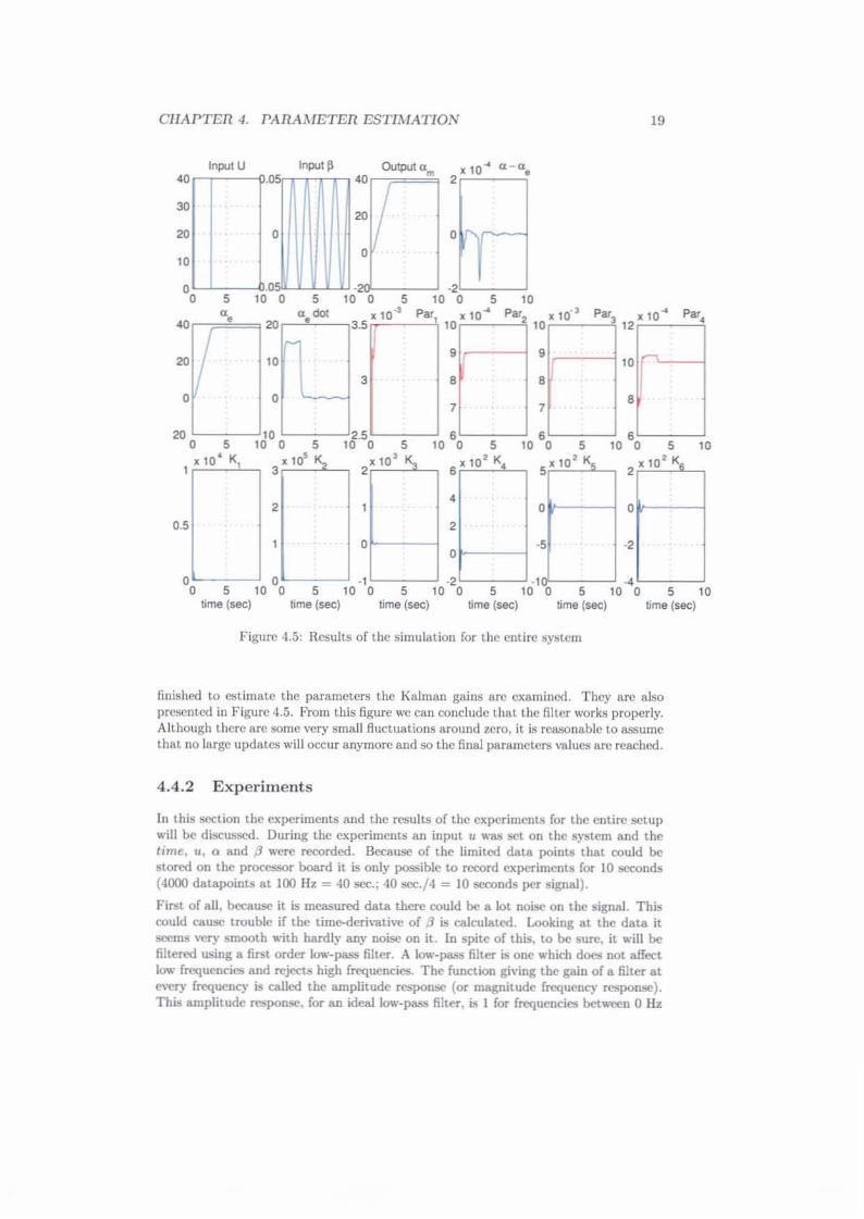
Figure 4.5: Results of the simulation for the elllire system

finished to estimate the parameters the Kalman gains are examined. They arc alsoprcscnted in Figurc 4.5. From this figure ....'C can conclude that the filter works properly.Although there arc some very small fluctuations around zero, it is reasonable to assumethat no large updates will occur anymore and so the final parameters values arc reached.

4.4.2 Experiments

In this section the experiments and the results of the expcrimelllS for thc entire setupwill be discussed. During the experiments an input II was set 011 the system and thetime, II, 0 and fJ were recorded. Because of the limited data points that could bestored on the processor board it is only possible to record experiments for 10 seconds(4000 dstapoints at 100 Hz = 40 sec.; 40 sec./4 = 10 seconds per signal).

First of all, because it is measured data there could be a lot noise on thc signal. Thiscould cause trouble if the time-derh-ative of (J is calculated. Looking at the data itsccms \"Cry smooth with hardly any noise on it. In spitc of this. to be sure. it will befiltered using a first order low-pass filter. A low-pass filter is one which does nOt affectlow frequencies and rejects high frequencies. The function giving the gain of a filter atever)' frequency is called the amplitude response (or magnitude frequency response).This amplitude response, for an idcallow.pass filter, is I for frequencies betlo\~n 0 Hz

CHAPTER 4. PARAMETER ESTIMATION 20

and the cut-off frequency, and it is 0 for all higher frequencies. The output spectrumis obtained by multiplying the input spectrum by the low-pass filter function.

The transfer function of the filter is:

( )0.15

Hz -----.".­- 1- 0.85z-1

The magnitude response IH(eiw)1 of the filter is:

IH(eiW)1 = 0.15V1- 1.7cosw + 0.852

Hence the cut-off frequency can be found:

w = 0.1048 rad/sample

f = 0.01667 cycle/sample

(4.12)

(4.13)

(4.14)

(4.15)

(4.16)

So this function has a cut-off frequency of 1.67 Hz at a sample frequency of 100 Hz.The Matlab function filtfilt is used for this filter. The data will first be filteredin forward .direction. This will lead to a phase-disturbance. To avoid this it will passthe filter twice. The second time in negative direction so zero phase-disturbance isobtained. All the data recorded is filtered. A small disadvantage is the fact that themagnitude of (3 will decrease a little bit. This may lead to a small error in the parameterestimation. But this error can be overcome and will hardly influence the final values.Not using this filter has shown that the EKF was not able to work. This means thelittle noise that is present in the signal was too much for these experiments.

The first data obtained from the experiments, in which a sine-function of 10 Hz wasput on the system, was not useful at all. The Kalman gains and the parameters didnot converge totally. It was even so that end values were depending on the given initialvalues for the covariance error matrix P and the noise intensity matrix R, which in factshould not make any difference and only affect the update speed of the parameters.

Another input is tried; just a step function in positive as well as negative directionwithin between a little break. Still depending on the initial conditions, the EKF evenestimated negative values for the friction this time, which is physical impossible.

This could be explained by the fact that the EKF method is based on linearisation.\Vhen a problem contains strong non-linear characteristics there may exist many localoptima. So when an experiment is started with different initial values it could bepossible that these several local optima causes different solutions.

The excitation of the pendulum is in all case larger than 1 rad, which is approximately58 degrees. This is a considerable angle in which it is to be expected that non-lineareffects will playa major role. We could avoid this by putting a short pulse (either pos­itive or negative) which magnitude is just above the dead-zone of the motor. Initially,this pulse will hit all the dynamics of the system before the free dynamical responsetakes over. Now the (3 becomes smaller than 0.6 rad and the Kalman filter wins moretime to converge to its right values. The results of these experiment are better butnot good yet. Although all the parameters are positive right now and the EKF gainsconverged to zero so now there is no physical update on the estimation anymore, theparameters have not converged to a stable value and still depend on the initial values.The length of the pulses varied from 0.5 to 1.0 to 1.5 seconds. The results of the pulses

CHAPTER 4. PARAMETER ESTIJ.1.ATION 21

-33 x 10

2

Par2

oH\r-----j

00);---<5---',.(0time (sec)

-2~0----.5,-----,-;('0time (sec)

Figure 4.6: Example of a parameter that has not con\1lrged while the correspondingKalman gain already did

of 1.0 and 1.5 seconds were far much better as the results of 0.5 seconds. This could beexplained with the fact that 0.5 seconds is much too short to excite all the dynamics.For example, it would probably just reach the border of the Coulomb friction so theviscous friction will not even play part in the dynamics.The last results were at least in the right direction. After observing the literature againit seems that the motor constants KJ::. and Kit· can be obtained in another wa)' aswell. This way, only three parameters have to be estimated (in-stead of four) whichgi\'cs the EKF more possibilities to estimate the dynamics of the system as well as theparameters in such a short time. The characteristics Kit Kb and Ro are givcn in thespecifications of the setup. Assuming they arc the same for both the motors these arc:

K, [I'm/AI 0.0706K b [Vs/cadl 0.0707

Ro [ohml 0.9

Table 4.4: Known motor characteristics

By measuring the voltage Vm that is send to the motor at a certain j>WM drivingcommand tJ the motor driver amplifiers gain J(u can be determined. The results ofthese experiments are shown in table 8.2 of appendix B. Here, just the average valuesare given.

Setup 1K.. IVjcountJ 0.0618

Setup 20.0682

Table 4.5: ~Icasurcd motor drive amplifier gain K ..

Now that the motor characteristics are known, new experiments arc done but now withpulse lengths of only 1.0 and 1.5 seconds. Again the magnitude of tJ is set just abo\1lthe dead·wne of the motor. 10 experiments arc done per time span, 5 in clockwisedirection (C) and 5 in counterclockwise dircc::tion (CC). The EKF seems to work farmore better now. as shown in Figure 4.7.

(4.17)

(4.18)

CHAPTER 4. PARAMETER ESTJjHATION 22

Inpul U Inpul ~ OUlpul<lm " -"m ,60 6 0.2

0.'40 4

0

20 2 o ,

0 , 0 O. 20 5 10 0 5 10 0 5 10 0 5 10

", <le dOl X10.3 ParI Par2 Par36 6 10 0.05 0.04

,fI\40044 0,03

2 6

2 0,03 0.020 4

0 2 2 0.02 0.010 , 10 0 , 10 0 , 10 0 , 10 0 , 10

30K,

300K,

0.'K,

0.2K.

0.2K,

200 0 020 0

'00 -0.2 -0.2

10 -0.5

0 1\

0 -0.4 -0.4

100 0' -0.6 -0.60 , 10 0 5 10 0 5 10 0 , 10 0 , 10

lime (sec) lime (sec) lime (sec) lime (sec) lime (sec)

Figure 4.7: Results of the EKF after reducing the number of parameters from 4 to 3

The results seems to be quite reasonable. To check these results the Least SquareMethod is used. The advantage of this method is that, givcn the model equations andmeasurement data, it will give the most suitable solution there is to fit the parameters.This is applied by using:

Where:

[ij ]A- a

- 1 - ~:h~+1 '

and,

y = -mll~&; - mllr&,sin2{3, ~ mI1oldJ;cos{3; - 2mllra'Plsin{3,cos{3,

'2 KtKu+1n l IOll{3. sin{3, +n;:-u

with i = datapoints. The derivatives of a and {3 will be calculated using the ccntraldifference method,

Both thc solutions for all the experiments are tabled in tables B.4 and B.6 of appendixB.

CHAPTER 4. PARAMETER ESTIMATION

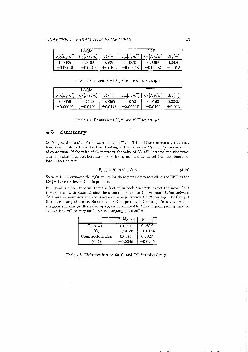
LSQM EKFJzo[kgm:l] Co [Ns/m] K f [-] JzO [kgm2 ] Co [Ns/m] Kf[-]

0.0035 0.0169 0.0351 0.0070 0.0268 0.0486±0.00021 ±0.0040 ±0.0166 ±0.00068 ±0.00637 ±0.012

Table 4.6: Results for LSQM and EKF for setup 1

LSQM EKFJzo [kgm2

] Co [Ns/m] Kf[-] Jzo[kgm2] Co [Ns/m] Kf[-]

0.0059 0.0140 0.0665 0.0052 0.0160 0.0569±0.00092 ±0.0106 ±0.0143 ±0.00237 ±0.0165 ±0.022

Table 4.7: Results for LSQM and EKF for setup 2

4.5 Summary

23

Looking at the results of the experiments in Table BA and B.6 one can say that theyhave reasonable and useful values. Looking at the values for Co and K f we see a kindof connection. If the value of Co increases, the value of K f will decrease and vice verse.This is probably caused because they both depend on a in the relation mentioned be­fore in section 2.2:

(4.19)

So in order to estimate the right values for these parameters as well as the EKF as theLSQM have to deal with this problem.

But there is more. It seems that the friction in both directions is not the same. Thisis very clear with Setup 2, since here the difference for the viscous friction betweenclockwise experiments and counterclockwise experiments are rather big. For Setup 1these are nearly the same. So now the friction present in the setups is not symmetricanymore and can be illustrated as shown in Figure 4.8. This phenomenon is hard toexplain but will be very useful while designing a controller.

I Co [Ns/m] I Kf[-] IClockwise 0.0161 0.0374

(C) ±0.0036 ±0.0134

Counterclockwise 0.0176 0.0327

(CC) ±0.0046 ±0.0205

Table 4.8: Difference friction for C- and CC-direction Setup 1

CHAPTER 4. PARAMETER ESTIMATION

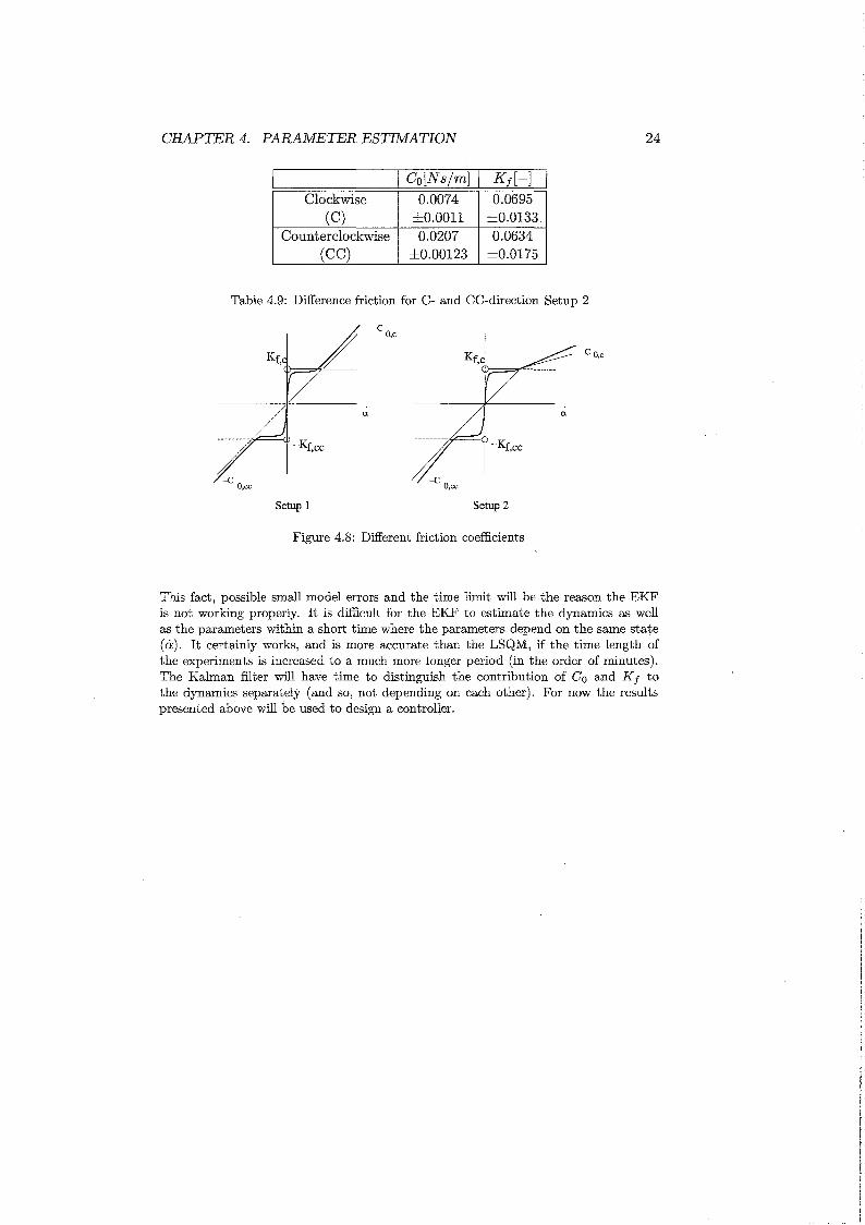
I Co [Nsjm] I K f [-] IClockwise 0.0074 0.0695

(C) ±0.001l ±0.0l33Counterclockwise 0.0207 0.0634

(CC) ±0.00l23 ±0.0l75

Table 4.9: Difference friction for C- and CC-direction Setup 2

24

--e O,cc

a

---------~

~o,cc

-Kf,cc

a

Co,c

Setup 1 Setup 2

Figure 4.8: Different friction coefficients

This fact, possible small model errors and the time limit will be the reason the EKFis not working properly. It is difficult for the EKF to estimate the dynamics as wellas the parameters within a short time where the parameters depend on the same state(a). It certainly works, and is more accurate than the LSQM, if the time length ofthe experiments is increased to a much more longer period (in the order of minutes).The Kalman filter will have time to distinguish the contribution of Co and K f tothe dynamics separately (and so, not depending on each other). For now the resultspresented above will be used to design a controller.

Chapter 5

Control of the pendulum

The goal of this project is to be able to balance the pendulum in upright position((3 = 7r). After studying some literature it seems a model-based linear controller willbe sufficient enough to control and balance the pendulum in upright position so noattention will be given to fuzzy controllers.

Since the pendulum is always in downward position when a balancing act is to beperformed it is obvious necessary to get the pendulum in upright position first. Thiswill be done with a swing up controller. This controller will swing up the pendulum tothe upright position, before a balancing controller will take over to keep the pendulumthere. In between a smart switching strategy has to be implemented so the balancingcontroller takes over at the right moment. Hence, the process of designing a controlleris divided in 3 parts:

• Swing up controller

• Switching strategy

• Balancing controller

5.1 Swing up controller

The swing up of the pendulum can be realized in different ways. One of these is to swingup the pendulum by energy control. This was first done by K.Furuta and K.J.Astrom.The entire theory behind this controller is already explained in [AstOO] and [Berg03]so this will not be mentioned again in this report. It is proved to work properly.

In this project Simulink is only used to perform simulations. In a dSPACE environmentthese files can be used to control the pendulum. Since no dSPACE environment isavailable for these setups, the programs have to be written in C++. To write the energybased controller in C++ is rather difficult and not really necessary. For this reason(and the reason that the objective of project is to balance the pendulum) just a simpleswing up controller (which is still a kind of derivative of the energy based controller)is implemented.

With this controller the pendulum starts in zero position ((3 = 0). The arm will givethe pendulum a small excitation. To give the pendulum a larger excitation, energyhas to be put into the system. This energy is inserted by movements of the arm.But it must be well timed and in the right direction because otherwise it will workagainst the swing up and will extinguish the excitation instead of increasing it. So the

25

CHAPTER 5. CONTROL OF THE PENDULUM 26

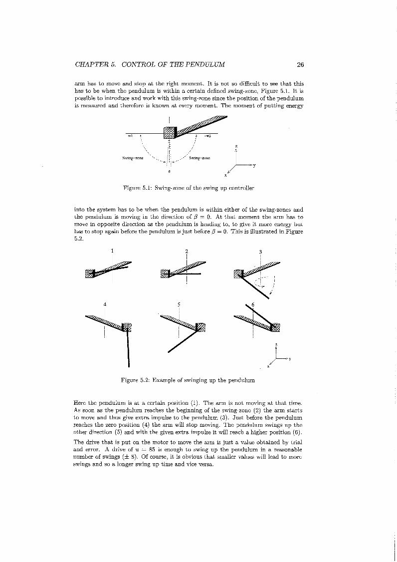
arm has to move and stop at the right moment. It is not so difficult to see that thishas to be when the pendulum is within a certain defined swing-zone, Figure 5.1. It ispossible to introduce and work with this swing-zone since the position of the pendulumis measured and therefore is known at every moment. The moment of putting energy

1[/2

Swing-zone

~','','','I /:1: ,.- ,~ Swing-zoneI_e-

"",,o

z

~_.yX

Figure 5.1: Swing-zone of the swing up controller

into the system has to be when the pendulum is within either of the swing-zones andthe pendulum is moving in the direction of j3 = O. At that moment the arm has tomove in opposite direction as the pendulum is heading to, to give it more energy buthas to stop again before the pendulum is just before j3 = O. This is illustrated in Figure5.2.

z

~yx

Figure 5.2: Example of swinging up the pendulum

Here the pendulum is at a certain position (1). The arm is not moving at that time.As soon as the pendulum reaches the beginning of the swing-zone (2) the arm startsto move and thus give extra impulse to the pendulum (3). Just before the pendulumreaches the zero position (4) the arm wlll stop moving. The pendulum swings up theother direction (5) and with the given extra impulse it will reach a higher position (6).

The drive that is put on the motor to move the arm is just a value obtained by trialand error. A drive of u = 85 is enough to swing up the pendulum in a reasonablenumber of swings (± 8). Of course, it is obvious that smaller values will lead to moreswings and so a longer swing up time and vice versa.

CHAPTER 5. CONTROL OF THE PENDULUM 27

In Figure 5.3 the result of an experiment with the swing up controller for setup 1 isshown.

driveu100

50

~~( \r~rf J~ n r~ ,~L~V! ! i lJ ~lrn--50

-100a 4arm position

100

50

vVVVV\~

i-50

_100'----'------L----'-----J::--~,_____--'------L---'

a 3 4

i:~~~:Jj\J~y1o 1 4

time(s)

Figure 5.3: Result of an experiment with the swing up controller

From these results it can be concluded that the controller works. Because no balancingcontroller was there yet to take over, the pendulum will continue its way, passes theupright position and returns to 00

• Later on, when a switching strategy and balancingcontroller are implemented this will not happen anymore. Notice two important aspectsof this plot. One, the discontinuity that is present in the graph of the pendulum positionis caused by the cross-over point. It is, as expected to be, located at -1070

. The peakpresent in the drive u is caused by this cross-over point but will not make any differencein swing-up. Second, the angle after 1800 continues increasing instead of decreasing.This is because the angle in the swing up controller is not normalized yet. In fact, thisis not really necessary because the controller will work with the number of counts fromthe potentiometer instead of the angle.

5.2 Switching Strategy

Now that it is possible to get the pendulum close to upright position the balancingcontroller has to keep it there. To activate the balancing controller a switching strategyhas to be implemented to switch from the swing up mode to balancing mode. So thisstrategy has to say when the balancing controller can take over form the swing upcontroller. It is almost impossible to switch when the pendulum is at exactly (3 = 'if

and since the balancing controller will have some range of attraction as well it is smartto choose a range of ±10 degrees from the vertical position to switch over from oneto another. So if the pendulum position is within 10 degrees (8 = 100

) from thevertical, the program will switch controller. In case the balancing controller "looses"the pendulum the swing up controller will be activated again. To prevent the controllerfrom chattering when the pendulum position is close to 10 degrees from the verticalthe switch-out point is placed lower than the switch-in point (i.e. 1=200

). See Figure5.4.

CHAPTER 5. CONTROL OF THE PENDULUM

Switch in~

I

28

Switch out/\ \ ~~ _ / I /~Switch out

\Y.-- / /\ ~ IY I\ I\ I

\\ 1/1

\ II\ II

Figure 5.4: Switching areas for the switching strategy

5.3 Balancing controller

The balancing controller is the most important part of this chapter. The controllerwill be based on the linearized model (around the equilibrium) and is a state feedbackcontroller. The disadvantage of a linearized controller is the limited region of attraction,but with the previous described switching strategy it should be good enough. Thecontrol law, u = -Kx, will be obtained using pole placement techniques.

5.3.1 Linearized model

The first step is to linearize the model around the unstable equilibrium [a a (3 ,B]T =[0 0 7r ojT. This is done in appendix E and hence the linearized model is:

Jzo + m1lii~mlloh

] [ ~ ] + [ Co +0KR~b ~l] [~ ] +

[0 0 ] [ a] [KtKU]o -mlgh (3 = ~a U

(5.1)

After rearranging and introducing some variables the state-space form is obtained:

with:

ac - b2

-cdo

-bd

(5.2)

a = Jzo + mll~

d = Co + KtKb

Ra

c = Jr1

f = KtKu

Ra

CHAPTER 5. CONTROL OF THE PENDULUM

and:

[10 0 O]r~l

y= 001 0 l~J

29

(5.3)

The matrix C is of the dimension [2 x 4] because both the arm and the pendulumposition are measured. From now on, all the used and defined parameters will onlyconcern setup 1. The design of the controller for setup 2 will be discussed later in thischapter. Substituting all known parameters into (5.2) the linearized state space modelbecomes:

raj ro 1

l~ l~ -~.1j3 0 -4.7

oS.lo

55.5

o ] r~l l01-Oi

021 l~ J + 1.~2 Ju-0.14 (3 1.01

(5.4)

6.A and 6.B are matrices that indicate how much deviation there is on these values.They are calculated with the values for the standard deviation on the parameters(chapter 4) using the chain and quotient rule.

o0.7o

0.6

o0.5o

0.4

o 1 l0 10.~02 J' 6.B = o.gs J0.05 0.06

The deviation, as can be seen in 6.A and 6.B, on the used system matrices is rathersmall. This means there will probably be no large influence from the deviation of theestimated parameters on the model.

5.3.2 Discrete time model

Since the setups work indiscrete time a discrete state feedback controller will be de­signed. The first thing to do is to convert the above described continuous time model toa discrete time model. To do so, the Matlab function c2dm will be used. The samplingtime and the 'method' have to be defined. The sampling time, T s = 0.01 seconds, isequal to the sampling frequency. The method used is the so-called 'zero-order hold'(zoh).

x(k + 1) = Adx(k) + BdU(k)

y(k) = Cdx(k)

(5.5)

(5.6)

la(k+1)]a(k + 1)(3(k + 1)J3(k + 1) l!

om0.94

-0.0002-0.045

0.0004O.OS

1.0030.553

o ] la(k)] l0.0001 ]0.0002 a(k) + 0.013 (k) (57)0.01 (3(k) 0 u .

1.001 J3(k) 0.01

CHAPTER 5. CONTROL OF THE PENDULUM 30

.6.A and .6.B will also be calculated for the discrete time model. Here the followingequation can be written:

eCA+L'.A)Ts = I + (A + .6.A)Ts + h.o.t.

= 1+ ATs + .6.ATs + h.o.t. (5.S)

These higher order terms (h.o.t.) contain T: with n 2:: 2 which will be equal to 10-4

or smaller. Since the term .6.ATs will be in the order of 10-3 these higher order termscan be neglected which will lead to the statement that .6.Ad = .6.ATs

For .6.Bd can be written:

oO.OOS

o0.006

o0.005

o0.004

~ l0.0~05 J

This leads to:

ro.OOOSl

.6.Bd = l 0.~05 J0.005

(5.9)

Again for A the deviation is rather small. This is not the case for B but since thevalues are pretty small (order of hand h2 ) it is reasonable to assume that also thediscrete time model will be representative for the system.

5.3.3 Incremental discrete time model

In addition to the present system an extra state variable u(k - 1) will be added to themodel resulting in an incremental model. This extra state variable implies that it iseffectively performing an integral action over all the other state variables. This gives apositive effect on the control law. The integrator will work as a kind of low-pass filterso the control signal will be smoother and constant errors will be filtered.

So now the state vector becomes:

r a(k) l[

x(k) ] l a(k) jxi(k) = u(k - 1) = ;~~?

u(k - 1)

The model can be written as:

xi(k + 1) = AdiXi(k) + B di .6.U(k)

y(k) = CdiXi(k)

(5.10)

(5.11)

CHAPTER 5. CONTROL OF THE PENDULUM

1 0.01 0.0004 0 0.0001[ 000010 0.94 0.08 0.0002 0.013 0.013

Adi = 0 -0.0002 1.003 0.01 0 Edi = 00 -0.045 0.553 1.001 0.01 0.010 0 0 0 1 1

31

To see if the obtained system is totally controllable and observable this will be checkedwith the controllability and observability matrices.

r 0.0001 0.0003 0.0006 0.00100015 ]l0013

0.025 0.036 0.047 0.057{} = 0 0.0002 0.0004 0.001 0.001 (5.12)

om 0.02 0.03 0.036 0.041 1 1 1 1

1 0 0 0 00 0 1 0 01 0.01 0.0004 0 0.00010 -0.0002 1.03 0.01 01 0.02 0.002 0 0.0003

(5.13)~-

0 -0.001 1.01 0.02 0.00021 0.027 0.003 0 0.00060 -0.002 1.025 0.03 0.00041 0.035 0.006 0.0001 0.0010 -0.004 1.04 0.04 0.001

Both these matrices are full of rank which proves the discrete time system is totallystate controllable and state observable.

To check the stability of the open loop response of the system, which is most likelyunstable, the poles of A di are calculated. These are:

1 +- a - integrator

1.0746 +- (3 - pole

0.9520 +- a - friction

0.9183 +- (3 - pole

1 +- u - integrator

Two ofthese poles are located at 1 and one at 1.0746. This confirms the intuition thatthe system is unstable in open-loop

5.3.4 Control law

The next step in designing a balancing controller is to find a control gains K. Thefirst assumption to be made here is that all five states are measurable. However,during the experiments this is not the case and only a and (3 can be measured andu(k - 1) is known. To obtain the needed Q and /3 an observer could be implemented.This not easily done in C++ and with the knowledge that the signals obtained from

CHAPTER 5. CONTROL OF THE PENDULUM 32

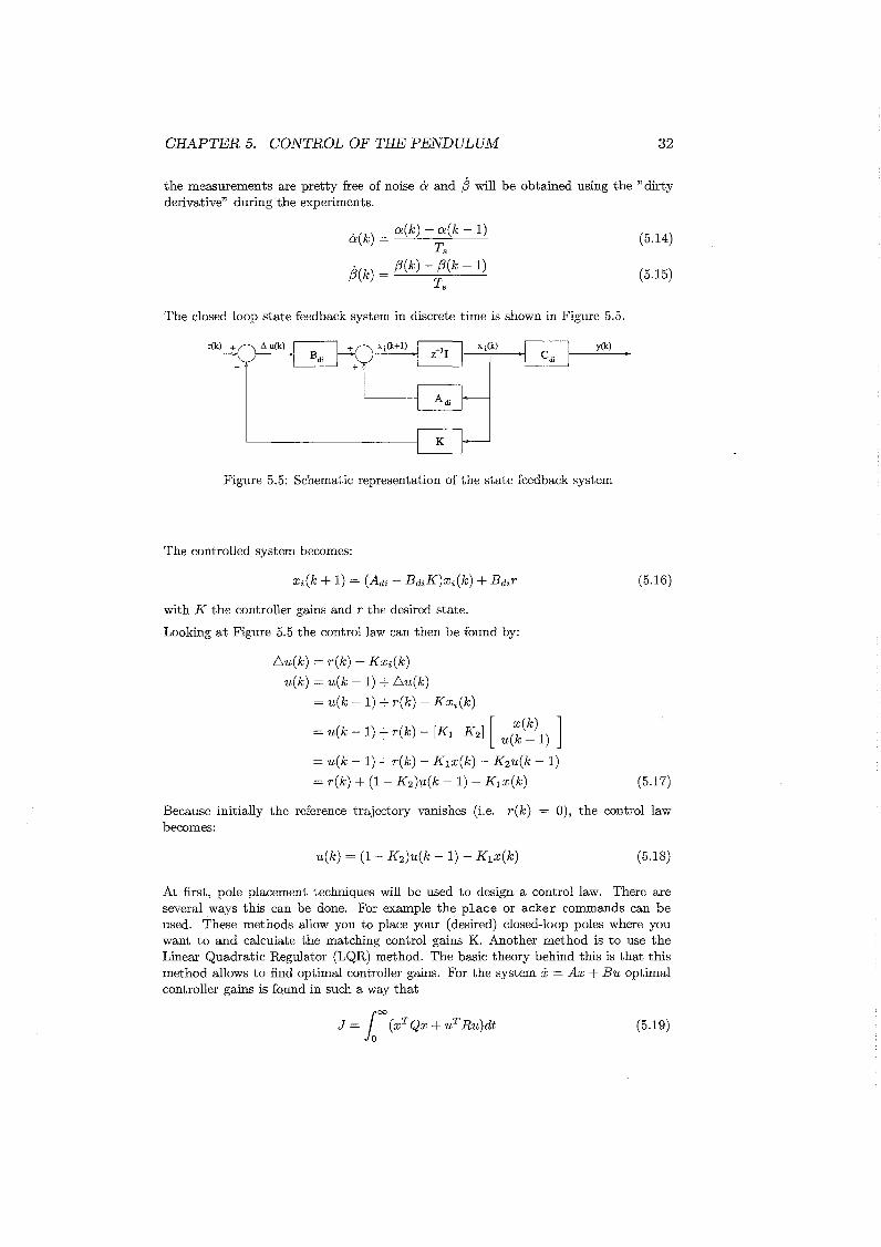
the measurements are pretty free of noise a and /J will be obtained using the" dirtyderivative" during the experiments.

a(k) = a(k) ~ a(k - 1)Ts

. (3(k) - (3(k - 1)(3(k) = T

s

The closed loop state feedback system in discrete time is shown in Figure 5.5.

Figure 5.5: Schematic representation of the state feedback system

The controlled system becomes:

with K the controller gains and r the desired state.

Looking at Figure 5.5 the control law can then be found by:

6u(k) = r(k) - KXi(k)

u(k) = u(k - 1) +6u(k)

= u(k - 1) + r(k) - KXi(k)

[x(k) ]= u(k - 1) + r(k) - [K1 K 2 ] u(k _ 1)

= u(k - 1) + r(k) - K1x(k) - K 2u(k - 1)

= r(k) + (1 - K 2 )u(k - 1) - K1x(k)

(5.14)

(5.15)

(5.16)

(5.17)

Because initially the reference trajectory vanishes (i.e. r(k)becomes:

0), the control law

(5.18)

At first, pole placement techniques will be used to design a control law. There areseveral ways this can be done. For example the place or acker commands can beused. These methods allow you to place your (desired) closed-loop poles where youwant to and calculate the matching control gains K. Another method is to use theLinear Quadratic Regulator (LQR) method. The basic theory behind this is that thismethod allows to find optimal controller gains. For the system x = Ax + Bu optimalcontroller gains is found in such a way that

(5.19)

CHAPTER 5. CONTROL OF THE PENDULUM 33

is minimized. Herc, R is thc performance tndex matnx and Q the .!tate-aMt matrix.The control law that minimizes J is givcn by linear State feedback u ::::: - K u. Onc canalso say that the optimal value of K is that which places the closed-loop poles at astable location.

To find suitable control gains, the parameters Q and R ha\'C to be specified. Forsimplicity R will be equal to R = 1. Q can be taken as Q = Cr.C••. The controllercan be tuned by changing these matrices to get a desirable response.

Sc\'t'f'81 comrollcr gains (K) have been calculated, tested (with thc help of a stcpfunction), and implemented into the setup but unfortunately none of them workedproperly. Once swung up in upright position the controller is not able to keep it therefor longer then I second caused by too large corrections on the actuated ann.

Ilov.'Cver. using pole placement techniques ha\'C helped to prepare a way in the rightdirection in order to find the gains of the control law whkh are able to balance thependulum. A trial and error method has been used to find them. After a lot ofexperiments with wrandom" (but tactical) chosen values, the \'slues of the gains tokeep the pendulum in upright position havc been found.

K ::::: [-6 - 5 137 20 0.16\

Thc results are plotted in Figure 5.6.

""

50 -~----''''''~':'-'''-----~---~----

i ,:'t?:-:....": "_.'~._M.,_:~ ...~jI.:~' : -~ .

0.. , . _.'_' .. l.l~l=:~'=1

D----~2,---------:.:--------:':------8::--------:':':D,-------"

l::f~'=_:_~~I'm:_.~I'~1-:-11700----~2,---------:.,---------:':--------:8::--------:':':O,------c"

"""Figure 5.6: Results of experiment controller for setup I: Perfect controlled

CllAPTER.5. CONTROL OF TilE PENDULUM 34

The plot starts at the moment the balancing controller took over from the s..... ing upcontrollcr. The pendulum is immediately in upright position and stays there. E\'en af­ter ± I second it is totally balanced and the controller does not ha\oc to correct the annposition (0). So the arm stands still. The fact that the dri\oc u is showing excitationin the plot is caused by a sort of bias offset. It is within the dead zone of the mOtor sothis won't havc any effect on the arm position. Unfortunately this is the perfect. case.~Iost of the times the results arc as plotted in S.7.

F'igure 5.7: Rcsults of experiment controller for setup I: Cood bllt less perfect COIl­

trolled

The results are reasonable. The fact that the controllcr is not able to keep the pen­dululll in perfect upright position is caused by the fact that in the beginning of everyexperiment the zero and upright position are defined. This upright position will alwaysbe the same and is obtained during the calibration. But for the zero position this isdifferent. Before statting an experiment the pendulum is at rest in downward position.This will be defined as the zero position. Due to some friction, this position doesn'th3\'e to be exactly at zero but for instance at -2 counts (virtual) but this is unknown.So now ~·2 = O~ and the new upright position is ~ -2 + upright position~ which is notexactly straight up but 0.70 from the \ocrtical. So now the controller thinks 179.30 isupright. Trying to balance it around this position it will always keep 011 moving dueto gravity. This is visualized is Figure 5.8.

This phenomena could be sol\'ed by letting the pendulum swing OUt after a - perfect­experiment. The end position is then known and the" 110\\'- upright position could be

CHAPTER 5. CONTROL OF THE PENDULUM 35

Perfect initial conditionuPJef

----1------ ---- cl _

Non-perfect initial conditionuPJef

downoup

,,,,,,ro

down

t,,,,,,o

up

Figure 5.8: Perfect initial condition

calculated easily. Unfortunately this is not possible at this moment since the controlprogram has to be loaded onto the setup every time you want to start an experimentand so the pendulum position will be reset every time.

Another thing that is remarkable is that the arm position moves around a certainpoint and tries to stay within a reasonable angle from this point. This is caused by thelinearisation of the arm position around O. Because of this the controller will alwaysaspire to bring the arm position back to O.

The values of the control gains that have been found by trial and error were imple­mented again in the model to see what the step response and the locations of the closedloop poles would be.

0.8731 + 0.3352i

0.8731 - 0.3352i

0.9372

0.9868 + 0.0172i

0.9868 - O.Ol72i

As we can see, the controller has to be smooth and robust. Perhaps, this can beexplained by the fact that the parameters that were estimated are not good enough todescribe the system.

Analyzing the stability radius of the continuous time system is an extra check wetherthe system is stable or not. The stability radius can be seen as the margin on .6.A andcan be defined as the largest singular value of the system:

(5.20)

Here E 1 and E z are the structure matrices and w is the eigenfrequency of the systemand will be investigated from 0 to 100 Hz. The stability radius has to be larger thanthe largest value in .6.A. Analyzing 2 different controllers (the first one is obtainedusing pole placement techniques, the second one by trial and error) the following radiiwere found:

K=K=

[-12 -7[-6 -5

99 14137 20

0.3]0.15]

St.rad. = 0.81St.rad. = 1.35

CHAPTER 5. CONTROL OF THE PENDULUM 36

....._-lQII-.. ;;:.;0'1

':r1

j"f~, .. ••••

".[

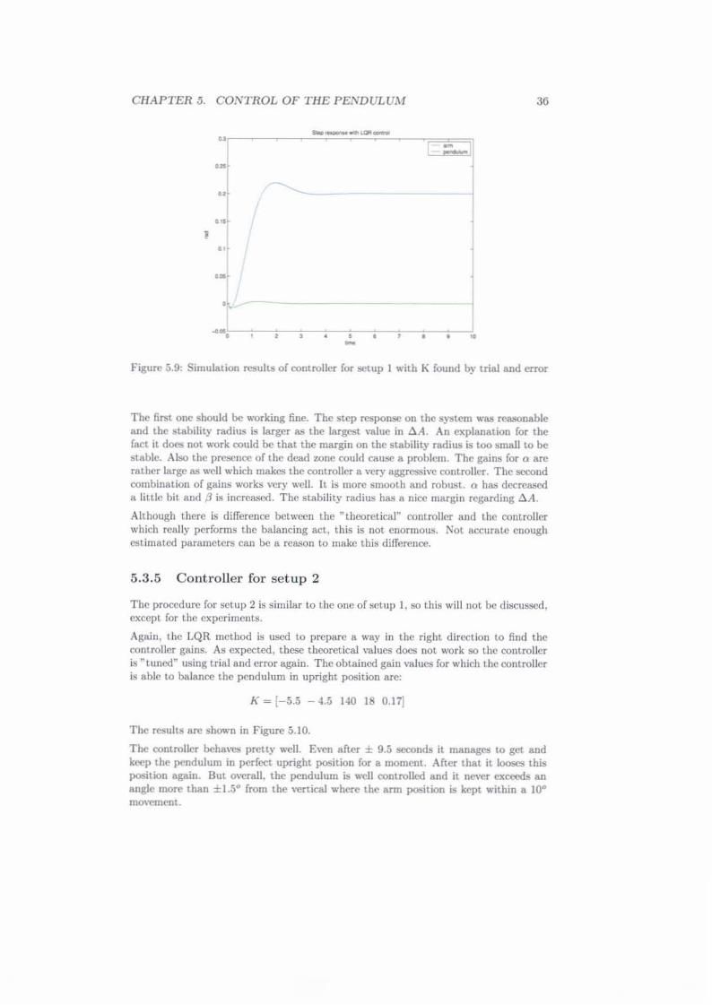
In, , • , , •-Figure 5.9: Simulation results of controller for setup I with K found by trial and error

The first one should be working fine. The step response on the system was reasonableand the stability radius is larger as the largest \'alue in 6A. An explanation for thefact it docs not ....-ark could be that the margin on the stability radius is too small to bestable. Also the presence of the dead zone could cause a problem. The gains for Q arerather large as well which makes the controller a very aggressive controller. The secondcombinalion of gains works very well. IL is more smooth and robust. 0 has decreaseda lillie bit and (3 is increased. The stability radius has a nice margin regarding 6A.

Although there is difference between the ~thcoretical" controller and the controllerwhich really performs the balancing act, this is not enormous. Not accurate enoughestimated parameters can be a reason to make this difference.

5.3.5 Controller for setup 2

The procedure for sctup 2 is similar to the one of sctup I, so this will not be discussed,except for the experiments.

Again, the LQR method is used to prepare a way in the right direction to find thecontroller gains. As expected, these theoretical \-alues docs not work so the controlleris ~tuned" using trial and error again. The obtained gain \-alucs for which the controlleris able to balance the pendulum in upright position are:

K = [-5.5 - 4.5 140 18 O.17J

The results are shown in Figure 5.10.

The controller behavcs prett)' well. E\"Cn after ± 9.5 seconds it manages to get andkeep the pendulum in perfect. upright position for a momClll. After that it looses thisposition again. But o\"CralL the pendulum is ...."CII controlled and it ne\"Cr exceeds anangle more than ±I.5° from the \"Crtical where the arm position is kept within 8 10"mo\"Cment.

CHAPTER 5. CONTROL OF THE PENDULUM 37

12

: .~

"Figure 5.10: Results of the experiments controller for setup 2

The elosed loop poles belonging to these values of the control matrix are:

0.9093 + 0.2585i

0.9093 - 0.2585i

0.9186

0.9885 + 0.0162i

0.9885 - 0.0162i

The l>tability radius for this last controller is calculated to be 1.46. Although the marginhere is not as large as the margin of the stability radius with sctup I, it is stable andpretty robust. Probably this can be explained with the fact that the dead·zone here isnot as big as in SCtup I and the parameters were better estimated.

CHAPTER 5. CONTROL OF THE PENDULUM

5.4 Summary

38

Now, two working controllers are designed. A controller which is able to swing up thependulum into upright position in a reasonable number of swings, a switching strategywhich switches from one controller to another at the right moment and a controllerwhich is able to keep the pendulum in upright position within a very close angle fromthe vertical (or sometimes even keeps it steady depending on the initial condition of /3)

The previous described differences of the blind and dead-zones in clockwise and counter­clockwise direction have been taken into account while writing the controller program.The differences in Co and K f in C and CC direction is hard to implement in C++. Thiswill certainly be possible in Simulink.

Chapter 6

Conclusions andRecommendations

6.1 Conclusions

Three months after the start of the projeet a lot of experience about the setup is gained.Improving the model, calibrating the encoders, estimating the parameters and design­ing and building a controller have been performed. Running against problems with theparameter estimation has been very useful to understand how the system works andhow they have to be solved. For the moment they can not be solved but once a dSPACEenvironment is build the method and files are ready to perform a new estimation. Con­cerning the design of a controller, a hybrid controller is build consisting of three parts;a swing-up, a switching and a balancing part. All these parts communicate so they cantake over from each other at the right moment. Pole placement techniques are usedto design the balancing controller but without succes. However, they have been veryuseful to search for those gains that are able to balance the pendulum. Although thecontrollers work properly and are able to keep the pendulum in upright position theycan be optimized once the correct parameters are known.

It can be concluded that it is possible to build a proper controller for a simple under­actuated system like the inverted pendulum. The experiences and files of this projectwill be useful for future projects with this setup.

6.2 Recommendations

Because of several reasons it is necessary to build a dSPACE environment for thesesetup. First of all, one can build a model in Matlab Simulink and convert it to dSPACE.This is more convenient than writing in C++. Second, it is possible to do longer exper­iments which seems to be necessary. And third, with dSPACE it is possible to controlboth setups" online" and at the same time.

Once dSPACE environment is build the parameters have to be estimated again and thegains of the controller have to be adapted. Once this is done it is possible to introducea reference trajectory. This reference trajectory defines a certain a or (3 the systemhas to follow. This could be a first step to future research on synchronization of thisunder-actuated system.

39

Bibliography

[Berg03]

[Fran94]

[Gelb74]

[Chye99]

[AstOO]

[Kuc79]

[web1]

H.W.J.v.d.Berg, Technical Report Traineeship University of Melbourne,2003, DCT report 2003.56

G.F.Franklin, "Feedback control of dynamic systems", 3rd editon,Addison-Wesley Publishing Company, 1994, ISBN: 0-201-53487-8

A.Gelb, "Applied Optimal Estimation", MIT Press, Cambridge (MA),1974

T.K.Chye and T.C.Sang, "Rotary Inverted Pendulum", Technical Re­port, School of Electrical and Electronic Engineering, Nanyang Techno­logical University, 1999

K.J.Astrom and K.Furuta, "Swinging up a pendulum by energy control",Automatica, volume 36 pp 287-295, 2000

V.Kucera, "Discrete Linear Control; the polynomial equation approach",Wiley, Chichester, 1979, ISBN: 0-471-99726-9

http:j jwolfrnan.eos.uoguelph.caj jzelekjmatlabjctms

40

Appendix A

Calibration Results

ISetup 1 I Setup 2 I

{3 = 0° I {3 = 180° {3 = 0° I {3 = 180"may. 1 0 508 0 546may. 2 0 505 2 547may. 3 0 506 2 543may. 4 -1 507 -2 545may. 5 0 506 0 545

Table A.1: Servo potentiometer calibration results Experiment 1

I Setup 1 I Setup 2 I{3 = 0° I {3 = 180° {3 = 0° I {3 = 180°

may. 1 0 507 0 540may. 2 0 508 1 541may. 3 0 507 0 540may. 4 0 507 0 545may. 5 0 505 0 545

Table A.2: Servo potentiometer calibration results Experiment 2

I Setup 1 I Setup 2 ,{3 = 90° I {3 = 270° {3 = 90° I {3 = 270°

may. 1 257 -255 274 -279may. 2 255 -258 274 -277mav.3 260 -256 275 -276may. 4 257 -255 274 -275mav.5 257 -255 274 -275

Table A.3: Servo potentiometer calibration results Experiment 3

41

APPENDIX A. CALIBRATION RESULTS 42

Setup 1exit cc entrance cc exit c entrance c

mov.1 -306 640 717 -306mov.2 -306 640 717 -306mov.3 -306 640 717 -306mov.4 -306 640 717 -306mov.5 -306 640 717 -306

Table A.4: Servo potentiometer calibration results Experiment 4 setup 1

Setup 2exit cc entrance cc exit c entrance c

mov.1 -322 701 701 -322mov.2 -322 701 701 -322mov.3 -322 701 701 -322mov.4 -322 701 701 -322mov.5 -322 701 701 -322

Table A.5: Servo potentiometer calibration resUlts Experiment 4 setup 2

1 A-C 44 43 44 48 48 45.41 A-CC -46 -41 -42 -44 -46 -43.81 B-C 45 46 45 46 46 45.61 B-CC -45 -45 -44 -44 -45 -44.62 A-C 27 29 28 28 30 28.42 A-CC -31 -32 -31 ---29 -29 -30.42 B-C 36 35 37 38 38 36.42 B-CC -38 -39 -39 -38 -38 -38.4

I Setup I Type I exp 1 I exp 2 I exp 3 I exp 4 I exp 5 I Average I

Table A.6: Results of motor dead zone experiment

Appendix B

Numerical Results of PEexperiments

Setup 1 Setup 2

exp 1 0.0959 x 10 3 0.7877 x 10 -3 0.1176 x 10 -3 0.7727 x 10 3

exp 2 0.1112 x 10 -;\ 0.7867 x 10 3 0.1199 x 10 -;\ 0.7700 x 10 3

exp 3 0.0905 x 10 3 0.7883 x 10 3 0.1204 x 10 3 0.7700 x 10 3

exp 4 0.0913 x 10 3 0.7886 x 10 3 0.1239 x 10 3 0.7705 x 10 3

exp 5 0.0888 x 10 3 0.7888 x 10 3 0.1216 x 10 3 0.7701 x 10 3

1 Average I 0.0955 x 10 3 I 0.7879 x 10 3 1 0.1207 x 10 3 1 0.7707 x 10 3 1

Table B.l: Results of parameters estimation Pendulum rod

I I Setup 1Drive Vm 1 K u

I Setup 2Vm I K u

40 2.10 0.0525 2.59 0.0648-40 -2.20 0.0550 -2.60 0.065050 2.90 0.0580 3.35 0.0670-50 -3.00 0.0600 -3.35 0.067060 3.75 0.0625 4.14 0.0690-60 -3.80 0.0633 -4.15 0.069270 4.50 0.0643 4.82 0.0689-70 -4.60 0.0657 -4.86 0.0694

1 Average 1__1 0.0618 1__1 0.0682 1

Table B.2: Results of voltage measurement

43

APPENDIX B. NUMERICAL RESULTS OF PE EXPERIMENTS 44

IExperiments I Direction I Time (s) I1-5 Clockwise (C) 1.0

6-10 Counterclockwise (CC) 1.011-15 Clockwise (C) 1.516-20 Counterclockwise (CC) 1.5

Table B.3: Experiments setup

Exp ----c;J,---zo---rI-L-S"""""'~;-OM-,-----~KC;O-f-iBr------O;;Jz-o-EKFCo

1 0.0038 0.0221 0.0226 0.0071 0.0347 0.04012 0.0037 0.0198 0.0311 0.0076 0;0337 0.03773 0.0035 0.0173 0.0268 0.0070 0.0283 0.04154 0.0036 0.0188 0.0252 0.0071 0.0305 0.03755 0.0034 0.0188 0.0216 0.0066 0.0292 0.03896 0.0036 0.0268 0.0185 0.0063 0.0382 0.03977 0.0036 0.0203 0.0154 0.0066 0.0304 0.03918 0.0033 0.0177 0.0257 0.0064 0.0270 0.04329 0.0033 0.0195 0.0135 0.0062 0.0289 0.0393

10 0.0036 0.0180 0.0198 0.0067 0.0279 0.038911 0.0035 0.0134 0.0516 0.0081 0.0237 0.053112 0.0033 0.0125 0.0403 0.0075 0.0205 0.059413 0.0032 0.0126 0.0568 0.0065 0.0197 0.062114 0.0033 0.0129 0.0499 0.0075 0.0221 0.052015 0.0033 0.0128 0.0481 0.0076 0.0213 0.058616 0.0040 0.0203 0.0724 0.0085 0.0369 0.039017 0.0037 0.0174 0.0617 0.0079 0.0302 0.043018 0.0035 0.0115 0.0359 0.0069 0.0174 0.070919 0.0033 0.0127 0.0209 0.0064 0.0182 0.068020 0.0032 0.0121 0.0436 0.0059 0.0166 0.0708

Average 0.0035 0.0169 0.0351 0.0070 0.0268 0.0486±0.0002 ±0.0040 ±0.016 ±0.0007 ±0.0064 ±0.012

Table B.4: Results of LSQM and EKF for setup 1

I Co [Ns/m] I K f [-] IClockwise 0.0161 0.0374

(C) ±0.0036 ±0.0134Counterclockwise 0.0176 0.0327

(CC) ±0.0046 ±0.0205

Table B.5: Difference friction for C- and CC-direction setup 1

APPENDIX B. NUMERICAL RESULTS OF PE EXPERIMENTS 45

ExpLSQM n EKF

r------;J;-zo--.I-C,=-o-----./--;OCK;-f-D-----;J;-zo--.------C,=o----.----K-;OC;-f----l

1 0.0051 0.0085 0.0517 0.0035 0.0034 0.07282 0.0052 0.0085 0.0605 0.0025 0.0039 0.08363 0.0051 0.0084 0.0582 0.0025 0.0035 0.08234 0.0052 0.0083 0.0610 0.0020 -0.0023 0.08965 0.0053 0.0082 0.0678 0.0001 -0.0069 0.10976 0.0068 0.0250 0.0530 0.0056 0.0231 0.05547 0.0070 0.0266 0.0557 0.0053 0.0235 0.06028 0.0071 0.0219 0.0640 0.0042 0.010 0.07719 0.0078 0.0387 0.0415 0.0080 0.0567 0.0233

10 0.0076 0.0419 0.0369 0.0077 0.0627 0.022311 0.0052 0.0067 0.0780 0.0037 0.0140 0.051512 0.0049 0.0062 0.0846 0.0061 0.0091 0.047913 0.0051 0.0058 0.0828 0.0042 0.0111 0.054214 0.0051 0.0069 0.0741 0.0044 0.0126 0.052115 0.0051 0.0067 0.0764 0.0042 0.0139 0.049216 0.0065 0.0131 0.0609 0.0080 0.0210 0.035917 0.0065 0.0120 0.0685 0.0082 0.0158 0.043918 0.0062 0.0094 0.0809 0.0079 0.0164 0.038419 0.0059 0.0091 0.0867 0.0080 0.0150 0.040620 0.0057 0.0090 0.0861 0.0076 0.0131 0.0470

Average 0.0059 0.0140 0.0665 0.0052 0.0160 0.0569±0.0009 ±0.011 ±0.014 ±0.0024 ±0.016 ±0.022

Table B.6: Results of LSQM and EKF for setup 2

ICo [Ns/m] I Kf[-] IClockwise 0.0074 0.0695

(C) ±O.OOl1 ±O'0133Counterclockwise 0.0207 0.0634

(CC) ±0.00123 ±0.0175

Table B.7: Difference friction for C- and CC-direction setup 2

Appendix C

Design of an EKF for thependulum rod

The design of an Extended Kalman Filter (EKF) starts with the equations of motion.These are already defined in section (4.3).

Only for the simulation an input u will be added so equation (C.l) will become:

(C.l)

(C.2)

but for the derivation of the EKF this will be ignored.

Define a vector ~ which represents the states and the parameters to be estimated.

and t. becomes:

Now the equation of motion can be written into state-space form.

l/J ] [ X2 1.. ~ "'2"'3 ~ mlgh. sin x

t. = iJz;.(t), t) = ~ = "'4 f4 1

Since we will only measure the position (3 of the system in this part of the estimationll(~(t), t) will be

ll(~(t),t) = [1 0 0 0]

46

APPENDIX C. DESIGN OF AN EKF FOR THE PENDULUM ROD 47

soz(t) = [I 0 0 0] x(t)

The Extended Kalman Filter is defined by:

;t = [(!K(t) , t) + K(£ - Mi, t)) (C.3)

P = F(i(t), t)P(t) + P(t)FT(i(t), t) + Q(t) - P(t)HT(i(t), t)R-1(t)H(i(t), t)P(t)(CA)

K(t) = P(t)HT(i(t), t)R-1(t) (C.5)

Now equation (C.3) can be written as:

In order to solve this K i has to be determined. K i can be solved from equation (C.5).But in order to solve this one equation (CA) has to be solved first.

F(:£, t) is the Jacobian of J(t) and so is H(:£, t) the Jacobian of h(t). So:

with:

m19hF1 = --- COS X lX4

X3F2 =--X4

X2F3 =--

X4

X2 X 3 m19h.F4 = -2- + --2- smx1

x 4 x 4

ahH(:£(t) , t) = ax. = [I 0 0 0]

J

(C.6)

(C.7)

(C.8)

(e.g)

R represents the matrix with measurement noise and its dimension is [lxI] becauseonly f3 is measured. So:

R=[R]

Q represents the model uncertainty and is defined as:

q13 q14]q23 q24q33 q34q43 q44

APPENDIX C. DESIGN OF AN EKF FOR THE PENDULUM ROD 48

P is the covariance error matrix and is symmetric.

To calculate P we have to calculate and integrate F. If (C.4) is calculated a set of socalled Ricatti equations are obtained.

2P12 + qll - R-1P[l

P 22 + F1Pn + F 2P 12 + F 3P 13 + F 4P 14 + q12 - R-1P n P 12

P 23 + q13 - R-1P n P 13

P 24 + q14 - R-1P n P 14

2F1P 12 + 2F2P22 + 2F3P23 + 2F4P24 + q22 - R-12P12

F 1P 13 + F2P 23 + F 3P33 + F4P 34 + q23 - R-1P 12 P 13

F 1P 14 + F 2P 24 + F 3P34 + F4P44 + q24 - R-1P 12P 14

q33 - R-12P13

q34 - R-1P 13 P 14

q44 - R-12P14

(C.IO)

(c.n)(C.12)

(C.13)

(C.14)

(C.15)

(C.16)

(C.17)

(C.18)

(C.19)

Now it is possible to calculate the Kalman gains with equation (C.5).

Now all equations are defined and ready to implement into Matlab Simulink. This isanalog to the pictures that will be presented in appendix D. This is done because theseare more interesting to see.

Appendix D

Design of an EKF for the totalsystem

D.l 2 states and 4 parameters

This part will in fact be the same as Appendix C but of course with other equations.Here the equation of motions are a little bit more difficult. They are already definedin section (4.4).

(D.I)

with:

K fh= 2[2[2 2(3J + /2 + /2· 2 f3 m 1 0 1 COSzO ml 0 ml 1 sln - Jr1

49

(D.2)

(D.3)

(D.4)

(D.5)

(D.6)

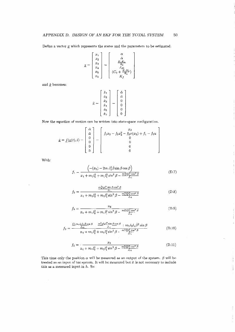
APPENDIX D. DESIGN OF AN EKF FOR THE TOTAL SYSTEM 50

Define a vector ;r which represents the states and the parameters to be estimated.

and i becomes:

;r=

0:

Q;K,KuR;;­Jzo

(Co + KR~b)

Kf

:i2=

a&oooo

Now the equation of motion can be written into state-space configuration.

With:

:i2 = [(;r(t) , t) =

( -(X5) - 2m1[i/3 sin (3 cos (3)h = -----''-------------;;2"'12"'"'12f--;;2--;;-(3

+ [2 + [2' 2 (./ m , a 1 cosX4 m1 0 m1 1 sm P - Jrl

X6is = --------=--------;;2"'12"'"'12.--;;2--;;-(3

+ [2 + [2' 2 (./ m , a 1 cosX4 m1 0 m1 1 Sln P - J

r1

C,m,lOht3 cos (3 + miglali sin (3 cos (3 + [[ /./2 . (./Jrl J r1 m1 0 1P Sln P

14 = 21212 2 (3

+ [2 + [2' 2 (./ m , a 1 cosX4 m1 0 m1 1 sm P - Jrl

X315 = 21212 2 (3+ [2 + [2' 2 (./ m , a 1 cos

X4 m1 0 m1 1 Sln P - Jr1

(D.7)

(D.S)

(D.9)

(D.lO)

(D.ll)

This time only the position a will be measured as an output of the system. (3 will betreated as an input of the system. It will be measured but it is not necessary to includethis as a measured input in h. So:

APPENDIX D. DESIGN OF AN EKF FOR THE TOTAL SYSTEM 51

ll(;r(t) , t) will be

ll(;r(t) , t) = [I 0 0 0 0 0 J

soz(t) = [I 0 0 0 0 0 J x(t)

Now equation (C.3) can be written as:

and

;r=

X2 + K 1 (z - Xl)h X 2 - hx~ - !3(J(X2) + 14 + i5u + K 2 (z - Xl)

K 3(z - Xl)K 4 (z - Xl)K 5 (z - Xl)K 6 (z - Xl)

with:

0 I 0 0 0 ;6 1F1 F2 F3 F4 F58r 0 0 0 0 0

~ jF(;r(t), t) =~ = 0 0 0 0 0Xj

0 0 0 0 00 0 0 0 0

o-X5 -2m,lol~/Jsin(3 cos (3 _ 2 m~loq sin (3eos 2(3x2 _ 4 x615e30x2

8, J r ,8, (e3ox2+1)28,

u8,

_ (-x5- 2m,lolf/Jsin(3cos(3)x2 + m~lolisin(3eos2(3x~ + x6(1-~)8~ J r ,8't 8't

mlloht2 sin!3+ °1 m1lJllt3 cos f3 + mr9l0l~sin f3 cos f3rl rl - W8r 8,-~8,

l-~

8,

H(;r(t) , t) = ::. = [I 0 0 0 0 0]J

(D.12)

(D.13)

(D.14)

(D.15)

(D.16)

(D.17)

(D.18)

R represents the matrix with measurement noise and its dimensions are [lxl] becauseonly a is used as a measured parameter. So:

R=[RJ

APPENDIX D. DESIGN OF AN EKF FOR THE TOTAL SYSTEM 52

Q represents the model uncertainty and is defined as:

qu q12 q13 q14 q15 q16

q2i q22 q23 q24 q25 q26

Q= q3i q32 q33 q34 q35 q36

q4i q42 q43 q44 q45 q46

q5i q52 q53 q54 q55 q56

q6i q62 q63 q64 q65 q66

P is the covariance error matrix and is symmetric.

Pu P12 P13 P14 P15 P16

rP"

P12 P13 P14 P15 P16

P2i P22 P23 P24 P25 P26 P12 P22 P23 P24 P25 P26

P=P3i P32 P33 P34 P35 P36 _ P13 P23 P33 P34 P35 P36

P4i P42 P43 P44 P45 P46- P

14 P24 P34 P44 P45 P46

P5i P52 P53 P54 P55 P56 P15 P25 P35 P45 P55 P56

P6i h2 P63 P64 P65 P66 L P16 P26 P36 P 46 P 56 P66 J

To calculate P we have to calculate and integrate P. If (C.4) is calculated a set of socalled Ricatti equations are obtained.

Pu 2P12 + qu - R- i P[i (D.19)

P12 P22 + FiPU + F2P12 + F3P13 + F4P14 + F5P15 + F6P16 + q12 - R- i PU P12

(D.20)

P13 P23 + q13 - R-i PU P13 (D.21)

A4 P24 + q14 - R-i PU P14 (D.22)

A5 P25 + q15 - R-i PU P15 (D.23)

A6 P26 + q16 - R-ip u P16 (D.24)

P22 2Fi P12 + 2F2P22 + 2F3 P23 + 2F4 P24 + 2F5P25 + 2F6P26 + q22 - R- 12P12

(D.25)

P23 F i P13 + F2P23 + F3P33 + F4P34 + F5P35 + F6 P36 + q23 - R- i P12P13

(D.26)

P24 F i P 14 + F2P24 + F3P34 + F4P44 + F5P45 + F6P46 + q24 - R- i P12P14

(D.27)

P25 F i P15 + F2P25 + F3P35 + F4P45 + F5P55 + F6P56 + q25 - R- i P12P15

(D.28)

P26 F i P16 + F2P26 + F3P36 + F4P46 + F5P56 + F6 P66 + q26 - R- i P12P15

(D.29)

APPENDIX D. DESIGN OF AN EKF FOR THE TOTAL SYSTEM 53

q33 - R-12P13

q34 - R-1P 13 P 14

q35 - R-1P 13 P 15

q36 - R-1P 13 P 16

q44 - R-12P14

q45 - R-1P 14 P 15

q46 - R-1P 14 P 16

q55 - R-12P15

q56 - R-1P 15 P 16

q66 - R-12P13

(D.30)

(D.3l)

(D.32)

(D.33)

(D.34)

(D.35)

(D.36)

(D.37)

(D.38)

(D.39)

Now it is possible to calculate the Kalman gains with equation (C.5).

(t) =

Pl1 1~2RP13

pR;. (t)

1{5 J~

R

Now all equations are defined and ready to implement into Matlab Simulink. This isshowed in figures D.l, D.3 and D.3.

Figure D.l: Main file of Kalman filter

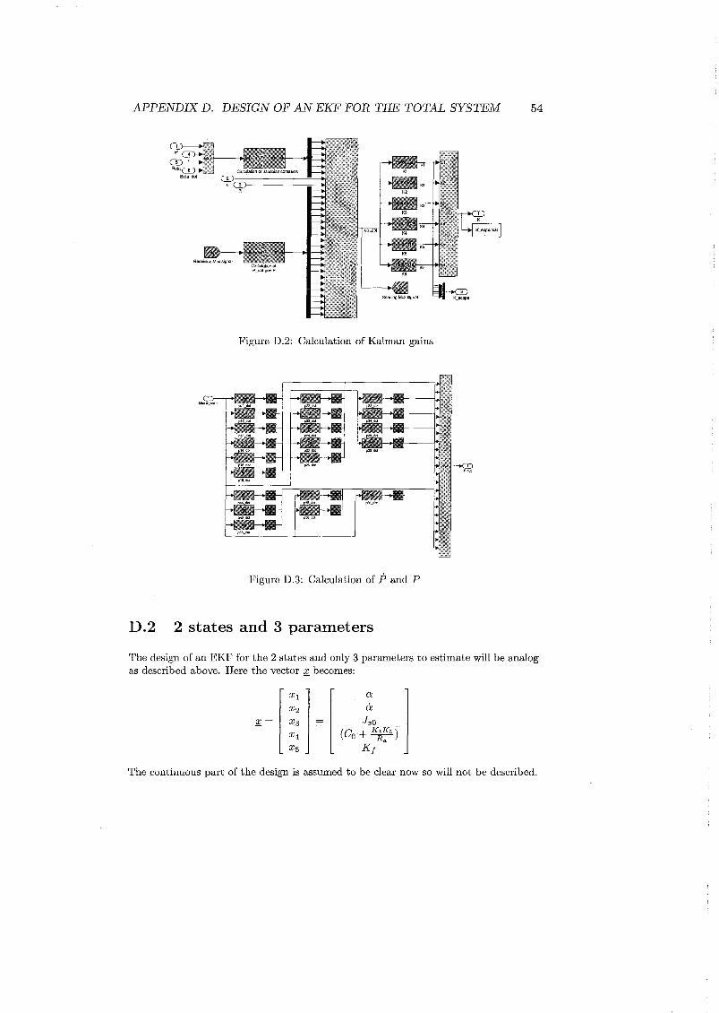
APPENDIX D. DESIGN OF AN EKF FOR THE TOTAL SYSTEM 54

Figure D.2: Calculation of Kalman gains

M"x.1gnalin

Figure D.3: Calculation of P and P

,,,,

D.2 2 states and 3 parameters

The design of an EKF for the 2 states and only 3 parameters to estimate will be analogas described above. Here the vector ± becomes:

The continuous part of the design is assumed to be clear now so will not be described.

Appendix E

Linearisation of the non-linearmodel

Here the linearisation of the non-linear model will be shown. The linearisation is basedon the expression of the non-linear function into a Taylor series about the operatingpoint and the retention of only the linear terms. For n variables, Xl, X2, •.• , X n it canbe briefly stated as:

Y=!(X1,X2""'Xn )

y = J(X1,X2' ... ,xn )

[ ~ ] +

[ ~ ] +

This looks difficult but in practice it is very easy to apply. Beginning with the non­linear model, this is defined as (2.23):

[Jzo + m1l6 + m1lr sin

2(3 m1lohCOS(3]

m1lohcos(3 JZ1 + m1lr

[Co + KIt,. + m1lr;3 sin (3 cos (3 m1lra sin (3 cos (3 - m1loh;3 sin (3 ]

-m1lra sin (3 cos (3 C 1

[~~;l:i:~ ]= [ K~~" ] U

(E.l)

This can be written as:

h (ex, a, (3,;3) = (Jzo + m116)i.i + m1Iri.isin2(3 + m110h,Bcos(3 + (Co + K~~b)a +

2 . '2 KtKu2m111 a(3sin(3cos(3 - m11011(3 sin(3 + Kj!J(a) - ~ua

(E.2)

55

APPENDIX E. LINEARISATION OF THE NON-LINEAR MODEL 56

Linearisation around the unstable equilibrium [0, 0, 7r, O]T for equation (E.2):

- 2 " .. KtKuil(O, 0, 7r, 0) = (Jzo + m110)a - m110h(3 - ~u

and:

8il ! = a8a <>=0,<'>=0,;3=7r,/3=0

0!1! . =Co+KtKboa <>=0,<'>=0,;3=7r,;3=0 Ra

oil! = a8(3 0<=0,<'>=0,;3=7r,/3=0

81.1 1 =00(3 <>=0,<'>=0,;3=7r,/3=0

Linearisation of (E.2) yields:

2 •• .• KtKb . KtKb(Jzo + m111)a - m110h(3 + (Co +~)a - ~u = a (E.4)

Linearisation around the unstable equilibrium [0, 0, 7r, OjT for equation (E.3):

12(0, 0, 7r, 0) = -m110hii: + Jrd3

and:

8121 =0oa 0<=0,<'>=0,;3=7r,/3=0

0121 =0oa <>=0,<'>=0,;3=7r,/3=0

o12!- . =-m1gh8(3 0<=0,<'>=0,;3=7r,;3=0

0~2! . = C10(3 0<=0,<'>=0,;3=7r ,;3=0

Linearisation of (E.3) yields:

-m110hii: + Jr1 ij - m1g11(3 + c1/3 = a

Hence, the linearized model is:

(E.5)

[Jzo + m115

-m110h ] [ ~ ] + [ Co +o¥ ~1] [~ ]+

[~ -m~gll] [ ~ ] = [ K~~u ] U (E.6) ,