Identification of Synchronous Generator model with Frequency ControlUsing Unscented Kalman Filter

Hossein Ghassempour Aghamolki, Zhixin Miao, Lingling Fan, Weiqing Jiang, Durgesh Manjure

Department of Electrical Engineering, University of South Florida, Tampa FL USA 33620.

Phone: 1(813)974-2031, Fax: 1(813)974-5250, Email: linglingfan@usf.edu.

Abstract

In this paper, phasor measurement unit (PMU) data-based synchronous generator model identificationis carried out using unscented Kalman filter (UKF). The identification not only gives the model of a syn-chronous generator’s swing dynamics, but also gives its turbine-governor model along with the primary andsecondary frequency control block models. PMU measurements of active power and voltage magnitude, aretreated as the inputs to the system while the measurements of voltage phasor angle, reactive power andfrequency are treated as the outputs. UKF-based estimation is carried out to estimate the dynamic statesand the parameters of the model. The estimated model is then built and excited with the injection of theinputs from the PMU measurements. The outputs of the estimation model and the outputs from the PMUmeasurements are compared. Case studies based on PMU measurements collected from a simulation modeland real-world PMU data demonstrate the effectiveness of the proposed estimation scheme.

Keywords: Synchronous Generator, Phasor Measurement Unite (PMU), Unscented Kalman Filter (UKF),Frequency Control, Droop Regulation

1. Introduction

Supervisory Control and Data Acquisition (SCADA) systems use nonsynchronous data with low densitysampling rate to monitor power systems. The measurements collected from SCADA can not capture thesystem dynamics. Phasor measurement units (PMUs) equipped with GPS antenna provide voltage andcurrent phasors as well as frequency with a high density sampling rate up to 60 Hz. PMU data can capturethe system electromechanical dynamics. In this paper, PMU data will be used for synchronous generatorparameter estimation.

Synchronous generator parameter estimation has been investigated in the literature. Based on the scopeof estimation, some only investigated electrical state estimation (e.g. rotor angle and rotor speed)[1, 2],while others estimated both system states and generator parameters [3–6]. Based on estimation methods,there are at least two major systematic methods for parameter estimation: least squares estimation (LSE)[7–9] and Kalman filter-based estimation [10–14]. To use LSE for dynamic system parameter estimation, awindow of data is required. On the other hand, Kalman filter-based estimation can carry out estimationprocedures at each time step. Thus Kalman filter-based estimation can be used for online estimation. Thisis also one of the reasons why PMU data-based system identification opts for Kalman filter-based estimation[10–14].

Kalman Filter was originally proposed for the linear systems. For nonlinear systems, there are twoapproaches to handle nonlinearity: extended Kalman filter (EKF) and unscented Kalman filter (UKF). InEKF, nonlinear systems are approximated by linear systems using linearization techniques. EKF was firstapplied by PNNL researchers in dynamic model identification using PMU data [5, 6, 10]. [5] focuses onparameter calibration for a simple generator dynamic model. [6] presents parameter calibration for a multi-machine power system under varying fault locations, parameter errors and measurement noises. In [10],parameter calibration for a more complicated generator model which includes electromechanical dynamics,

Preprint submitted to Electric Power Systems Research April 26, 2015

electromagnetic dynamics, exciter dynamics, voltage control blocks and power system stabilizer (PSS), waspresented. EKF-based simple generator model estimation was also carried out in [11, 12]. Limitations ofEKF method has also been investigated in [11].

In UKF, a nonlinear system model will not be linearized. The stochastic characteristic of a randomvariable is approximated by a set of sigma points. This technique is essentially Monto-Carlo simulationtechnique. Dynamic process of these sigma points will be computed based on the nonlinear estimationmodel. Statistic characteristics of the dynamic process will then be evaluated. UKF can overcome thelimitation of the linearization process required by the EKF method. However, more computing effort isrequired due to the introduction of sigma points. In [13], UKF is applied for state estimation. Accuracyand convergence for both EKF and UKF are compared in [13]. This paper focuses on state estimation only.Parameter estimation was not discussed. In [14], UKF is applied to estimate the following parameters Eq,x′d and H along with states. A comparison of various Kalman filter methods is documented in [15].

The synchronous generator model identified in the aforementioned papers focuses on the generator elec-tromechanical, electromagnetic and excitation system only. For example, a 4th order transient generatorestimation model is assumed in [15]; a subtransient generator estimation model is adopted in [10]. None hasaddressed frequency control system identification. The goal of this paper is to apply UKF for parameter andstate estimation for a synchronous generator model consisting of electromechanical dynamics and frequencycontrol. Contributions of this paper are summarized in the following paragraphs.

• Not only electromechanical dynamics related states and parameters, but also turbine-governor dy-namics, primary and secondary frequency control parameters will be estimated. Estimation related tofrequency control based on PMU data has not been seen in the literature.

Particularly, we will estimate the following parameters and states: inertia constant H, damping factorD, internal voltage Eq, transient reactance x′d, mechanical power input Pm, Droop regulation R,turbine-governor time constant Tr, and secondary frequency control integrator gain Ki.

Some parameters are difficult to estimate due to nonlinearity. Parameters conversion is adopted inthis paper in order to make estimation easier.

• Event playback method [10] is used in this paper to validate the identified low-order model. Forvalidation, estimated parameters will be used to create a dynamic simulation model. Then eventplayback will be used to inject the same inputs to the dynamic simulation model. The output signalsfrom the simulation will be compared with the PMU measurements.

• Lastly, real-world PMU data-based identification will be used to demonstrate the effectiveness of theproposed estimation model.

This paper is organized as follows. Following a description of basics of UKF algorithm in Section 2,the implementation of UKF for dynamic generator model estimation is discussed in Section 3. Section 4presents the validation process and case studies. Finally, Section 5 presents the conclusions of this paper.

2. Basic Algorithm of UKF

A continuous nonlinear dynamic system is represented by the following equations.{x(t) = f [x(t), u(t), v(t)]

y(t) = h[x(t), u(t), v(t)] + w(t)(1)

where, x(t) is the vector of state variables, y(t) is the vector of output variables, u(t) is the vector of inputvariables, v(t) is the non-additive process noise, and ω(t) is additive measurement noise. Considering thetime step of ∆t, (1) can be written as (2) in the discrete time domain:

2

xk = xk−1 + f [xk−1, uk−1, vk−1]∆t

= f [xk−1, uk−1, vk−1]

yk = h[xk, uk, vk] + wk

(2)

The state xk is considered as a random variable vector with an estimated mean value xk and an estimatedco-variance Pxk

. Vector ψk is considered as a set of unknown model parameters. For simplification, ψk can

also be treated as states, where ψk+1 = ψk. Then , the new state vector is Xk =[xk

T ψkT]T

. Thestate-space model in (2) is reformulated as:{

Xk = f [Xk−1, uk−1, vk−1]

yk = h[Xk, uk, vk] + wk(3)

Kalman filter is a recursive estimation algorithm. At each time step, given the previous step’s information,such as the mean of the state Xk−1, the covariance of the state PXk−1

, Kalman filter estimation will provide

the statistic information of the current step, i.e., the mean of the state Xk and the covariance of the statePXk

. Usually a prediction step estimates the information based on the dynamic model only, and a correctionstep corrects the information based on the current step’s measurements. There are several references forUKF algorithm in literatures. For rest of this section, [16] is the reference for all UKF algorithm relatedequations.

Unscented Kalman filter (UKF) is a Monte-Carlo simulation method. A set of sigma points will begenerated based on the given statistic information: mean and covariance of the states. Sigma points vectorswill emulate the distribution of the random variable. The set of sigma points is denoted by χi and theirmean value represented by X while their covariance represented by PX . For n number of state variables, aset of 2n+ 1 points are generated based on the columns of matrix

√(n+ λ)PX . As shown below, at k − 1

step, 2n+ 1 sigma points (vectors) are generated.χ0k−1 = Xk−1

χik−1 = Xk−1 +[√

(n+ λ)PXk−1

]i, i = 1, ..., n

χi+nk−1 = Xk−1 −[√

(n+ λ)PXk−1

]i+n

, i = 1, ...., n

(4)

where λ is a scaling parameter (λ = α2(n+ κ) − n), α and κ are positive constants. In the prediction step,prediction of the next step state will be carried out for all these sigma points. Based on the information ofthe sigma points of the next step, the mean and the covariance of the states will be computed. UKF willuse weights to calculate the predicted mean and covariance. The associated weights are as follows.

Wm0 = λ

(n+λ)

Wc0 = λ(n+λ) + (1 − α2 + β)

Wmi= 1

2(n+λ) , i = 1, ..., 2n

Wci = 12(n+λ) , i = 1, ..., 2n

(5)

where β is a positive constant, Wmiis used to compute the mean value, and Wci is used to compute the

covariance matrix. α, κ and β are the Kalman Filter parameters which can be used to tune the filter.Scaling parameter β is used to incorporate prior knowledge of the distribution of x(k) and for Gaussiandistribution β = 2 is optimal [hyun2011]. The scaling parameter α is a positive value used for an arbitrarysmall number to a minimum of higher order effects. To choose α, two laws have to be take into accounts.First, for all choices of α, the predicted covariance must be defined as a positive semidefinite. Second, Theorder of accuracy must be preserved for both the mean and covariance [17]. See [18] and [17] for moredetails regarding the effect of scaling parameter α on UKF tuning. In this case study, we have chosen

3

α = 10−4, β = 2.κ is a scaling factor that controls how far away from the mean we want the points to be. A larger κ will

enable points further away from the mean be chosen, and a smaller κ enables points nearer the mean to bechosen. Based on Equation (5), it can be also seen that when κ gets larger, not only the sampled sigmapoints go further away from the mean, but also the weights of those samples get smaller. In another word,by choosing a larger κ, samples are chosen further and further away from mean with less weight assignedto those samples. Therefore, choosing appropriate κ will reduce higher order errors of Tylor’s series forpredicting the mean and covariance of the states of the system. It is shown in [19] and [20], that if x(k)is Gaussian, it is more appropriate to choose κ in a way that n + κ = 3. However, if the distribution ofx(k) is different, then we have to use different approach for choosing κ. Detailed discussion regarding UKFparameters can be found in [19–21]. In this case study, we choose κ = 0 since we use total 7 sigma pointand n = 3.

The predicted sigma points at the k-th step (χ−k ), the mean (X−k ) and the covariance (P−Xk) of the k-th

step state are described in (6). Note the superscript − denotes a prior state or prediction.

χi−k = f(χik−1, uk−1), i = 0, · · · , 2n

X−k =2n∑i=0

Wmiχi−k

P−Xk=

2n∑i=0

Wci

(χi−k − X−k

)(χi−k − X−k

)T (6)

Subsequently, the predicted measurement sigma points γ−k can be generated by finding the predictedsigma points χ−k through the measurement equation (7).

γi−k = h(χi−k , uk), i = 0, · · · , 2n (7)

Consequently, the weighted mean of the predicted measurement y−k and the corresponding covariancematrix P−yk as well as the cross-correlation matrix P−Xkyk

can be computed as shown in (8).

y−k =2n∑i=0

Wmiγi−k

P−yk =2n∑i=0

Wci(γi−k − y−k )(γi−k − y−k )T +Rw

P−Xkyk=

2n∑i=0

Wci(χi−k − X−k )(γi−k − y−k )T

(8)

where Rw is the co-variance matrix related to the measurement noise w. In the correction step, UKFthen updates the state using Kalman gain matrix Kk. The mean value Xk and co-variance matrix PXk

(superscript − denotes a prior state) are expressed as follows.

Kk = P−Xkyk

(P−yk)−1

Xk = X−k +Kk

[yk − y−k

]TPXk

= P−Xk−KkP

−ykKTk

(9)

There are existing general Kalman filter Matlab toolboxes available. In this research, we use a generalEKF/UKF toolbox developed by Helsinki University [22]. Specific models of PMU data-based synchronousgenerator estimation are described in the next section and coded in the toolbox.

4

3. Implementation of UKF for dynamic model parameter estimation

In the proposed estimation model, a synchronous generator is considered as a constant voltage sourcebehind an impedance. The electromechanical dynamics can be described by the following swing equation[23]. {

dδ(t)dt = ωs(ω(t) − ω0)dω(t)dt = 1

2H (Pm − Pg(t) −D(ω(t) − ω0))(10)

where δ(t), ω(t), ω0 and ωs are the rotor angle in radius, rotor speed in pu, synchronous speed in pu andbase speed (377 rad/s), respectively. Rewriting the dynamic equations in the discrete form, we will have:{

δk = δk−1 + (ωk−1 − ω0)ωs∆t

ωk = ωk−1 + ∆t2Hk−1

(Pmk−1− Pgk−1

−Dk−1(ωk−1 − ω0))(11)

where ∆t is the sample period. The PMU measured data can be separated into two groups. One groupis treated as the input signals to the dynamic model and the other group is treated as the outputs ormeasurements. A PMU provides five sets of data at a generator terminal bus: voltage magnitude (Vg),voltage phase angle (θ), active power (Pg), reactive power (Qg), and frequency (f). The PMU data containsonly the positive sequence in this application based on the assumption that the system is operated underbalanced conditions. Based on the swing equation, the state vector of the system is defined as xk = [δk ωk]T .If we treat the parameters (unknown mechanical power Pm, inertia constant H and damping coefficient D)of the model as state variables, the augmented state vector will be Xk = [δk ωk Pmk

Hk Dk]T .In this paper we will use terminal voltage magnitude (Vg) and generator exported power (Pg) as the

input signals, the terminal voltage phasor angle (θ) together with the reactive power are treated as theoutput signals. The relationship between input and output signals can be written as follows.Pg =

EqVg

x′dsin(δ − θ)

Qg =EqVg cos(δ−θ)−V 2

g

x′d

(12)

From (12) we can write:

{EqVg sin(δ − θ) = Pgx

′d

EqVg cos(δ − θ) =√

(EqVg)2 − (Pgx′d)2

(13)

Based on (13), the output signals can be expressed by the input signals and state variables as follows.θgk = δk − tan−1

(Pgk

x′dk√(Eqk

Vgk)2−(Pgk

x′dk)2

)Qgk =

√(Eqk

Vgk)2−(Pgk

x′dk)2−V 2

gk

x′dk.

(14)

3.1. Primary and Secondary Frequency Control

In the case that a system loses its power balance, the primary frequency control of synchronous generatorswill adjust the mechanical power reference point to a new value based on the frequency deviation. Theprimary frequency control is composed of a proportional block with the deviation of frequency as the input,the change in the mechanical power reference as the output. If the frequency is below the nominal value,the mechanical power should be increased. Otherwise, the mechanical power will be decreased. The systemfrequency will achieve steady state after such compensation. However, the steady-state frequency will deviatefrom the nominal value. Secondary frequency control loop is then added in order to bring the frequencyback to its normal value. The secondary frequency control is mainly composed of an integral block as shown

5

in Fig. 1. The integral unit senses the deviation in frequency or rotor speed and adjusts the reference powerPc. This way, the generator will be able to adjust its power input responding to the system load change.

In Fig. 1, R is the speed regulation constant, 1R is named as the droop gain, and Tr is the turbine-governor

time constant. Additional dynamic equations are as follows after considering the frequency controls.

dPmdt

=1

Tr

(Pref − Pc − Pm − 1

R(ω − ω0)

)(15)

Rewriting (15) in the discrete form, we have:

Pmk= Pmk−1

+∆t

Tr

(Pref − Pck−1

− Pmk−1− 1

R(ωk−1 − ω0)

)(16)

Similarly, the secondary frequency control can be written as:

Pck = Pck−1+ (ωk−1 − ω0)Kik−1

∆t. (17)

The state vector of the system is now defined as xk = [δk ωk PmkPck ]T . If we treat the parameters of

the model as state variables, the augmented state vector will be Xk = [δk ωk PmkPck Rk Kik Hk Dk]T .

The complete generator estimation model is presented as follows.

δk = δk−1 + (ωk−1 − ω0)ωs∆t

ωk = ωk−1 + ∆t2Hk−1

(Pm − Pgk−1+Dk−1(ωk−1 − ω0))

Pmk= Pmk−1

+ ∆tTrk

(Pref − Pck−1

− Pmk−1− 1

Rk(ωk−1 − ω0)

)Pck = Pck−1

+ (ωk−1 − ω0)Kik−1∆t

Rk = Rk−1

Kik = Kik−1

Hk = Hk−1

Dk = Dk−1

Trk = Trk−1

(18)

The model will be adapted for PMU data-based estimation to enhance the convergence of the UKFalgorithm. Some parameters will be converted to new parameters in the estimation process. The detailedconversion will be shown in Case Studies. Parameter conversion has also been adopted in the literature [14].

4. Case Studies

4.1. Case Study Based On Simulation Data

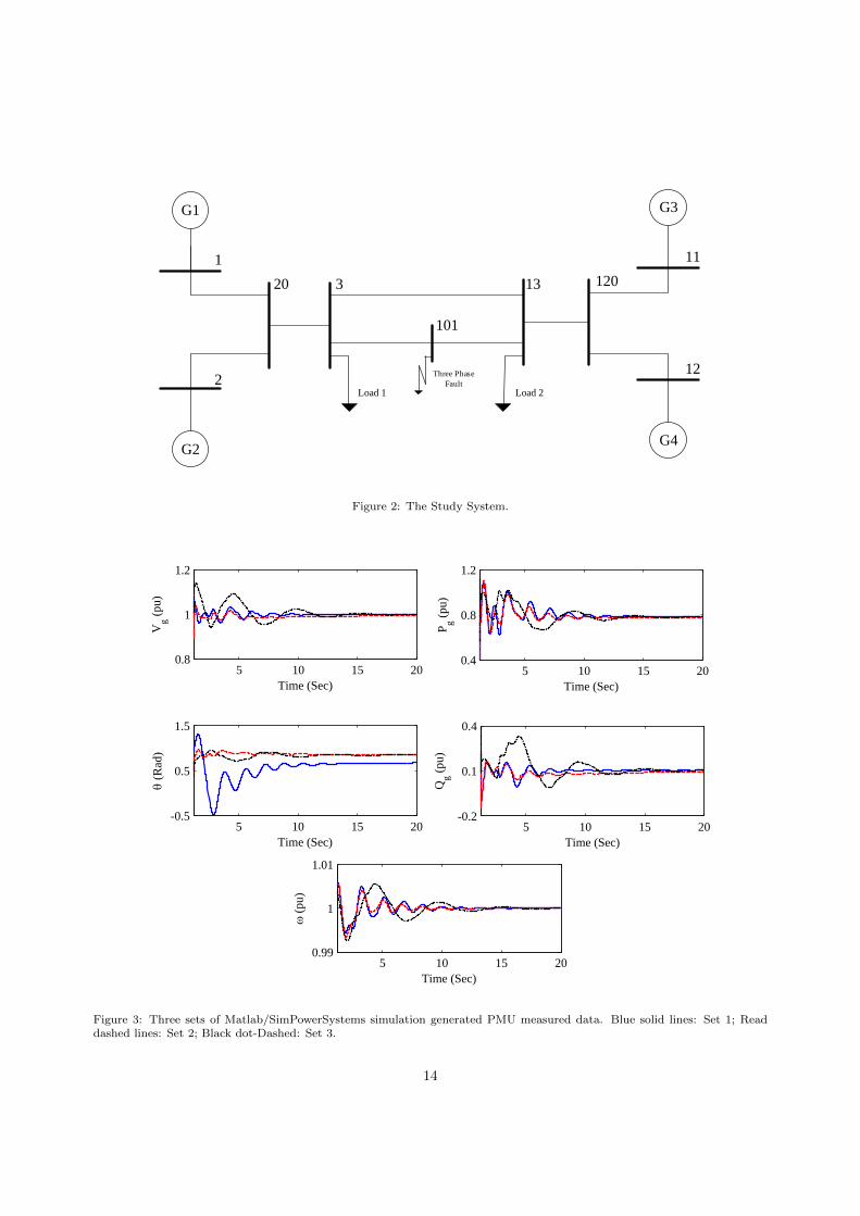
To generate PMU data for case study, time-domain simulation data is generated using Matlab/SimPowerSystems.Demos in Matlab/SimPowerSystems include a classic two-area nice-bus system [23] shown in Fig. 2. Thissystem consists of four generators in two areas. Two tie-lines connect these two areas. At t = 1 second, athree-phase low impedance fault occurs at Bus 101. After 0.2 second, the fault is cleared. A PMU is usedto record power, voltage, and the frequency data from the terminal bus of Gen 1. The sampling interval is0.01 second.

Three sets of data were recorded (shown in Fig. 3) and used to test UKF method. Each set of datarepresents a different model for Generator 1 in the simulation studies.

• Set 1: For benchmarking, the classical generator model ( a constant voltage source behind a transientreactance) is used in simulation. In this case, the dynamic model used in UKF is exactly the same asthe simulation model.

6

• Set 2: A subtransient model which includes all damping winding dynamics is used to representGenerator 1 in simulation. In the estimation model, dynamics related to the flux and damping windinghave all been ignored.

• Set 3: The power system stabilizer (PSS), automatic voltage regulator (AVR), and excitation systemare added to the subtransient generator model in this simulation. Adding PSS, AVR, and excitationsystem adds transients to the internal voltage of generator (Eq). In the estimation model, Eq isassumed to be constant.

In addition, turbine-governor, primary and secondary frequency control models same as those in theestimation model have been considered in Matlab/SimPowerSystems-based simulation. The generator pa-rameters can be found in Table 5. At least two initial guesses for each parameter will be used to demonstratethat UKF can converge to the same estimation.

Parameter Conversion. In the process of UKF tuning, we found that direct estimation of R, Tr and H leadsto decreased rate of algorithm convergence. From (18), it can be anticipated that the state variables ω andPm are linearly related to 1

2H , 1R and 1

TrRrespectively. Therefore, a small change in R, Tr and H results

in big fluctuations in Pm and ω. In other words, the output measurements have insignificant sensitivity tothe parameters R, Tr and H, which makes the filter tuning very difficult. To address this issue, parametersG = 100

2H , J = 1TrR

and N = 1Tr

will be estimated. With such changes, ignoring the damping coefficient (D),(18) can be rewritten as (19).

δk = δk−1 + (ωk−1 − ω0)ωs∆t

ωk = ωk−1 + Gk−1

100 (Pm − Pgk−1)∆t

Pmk= Pmk−1

+Nk−1(Pref − Pck−1− Pmk−1

)∆t− Jk−1(ωk−1 − ω0)∆t

Pck = Pck−1+ (ωk−1 − ω0)Kik−1

∆t

GK = Gk−1

MK = Mk−1

JK = Jk−1

Kik = Kik−1

(19)

In the literature, V , θ, P , and Q of PMU data are used as an input-output for Kalman Filter [5, 11, 14].However, in this paper, frequency control parameters are to be estimated. Based on our experience, withoutfrequency measurements from the generator terminal bus, convergence of the estimation is problematic.Therefore, the frequency of generator terminal bus is recorded and used as an output. We also make asimplifying assumption that the frequency measured at the generator terminal bus is equivalent to the rotorspeed (ω) in per unit. The output signals can be written by input signals and state variables in the discreteform as follows.

θgk = δk − tan−1

(Pgk

x′dk√(Eqk

Vgk)2−(Pgk

x′dk)2

))

Qgk =

√(Eqk

Vgk)2−(Pgk

x′dk)2−V 2

gk

x′dk

fk = ωk

(20)

For this estimation model, Eq, Pref , x′d are assumed known. In the UKF algorithm, P is the co-variance

matrix of the state variables, X0 is the initial guess of the augmented state vector and P0 is the initial guessfor the co-variance matrix P . Estimation accuracy is not sensitive to the initial guess of parameters or statevariables. Initial guess for covariance matrix (P0) will influence the convergence rate. Therefore, fine tuningof P0 is needed. Q is the co-variance matrix of the process noise and kept constant for all three sets of data.Table 1 shows the initial guess for X0 and P0 as well as diagonal elements of process noise matrix Q. Rw isthe covariance matrix of the output measurement noise (Rw = diag

(10−15 10−15 10−15

)) .

7

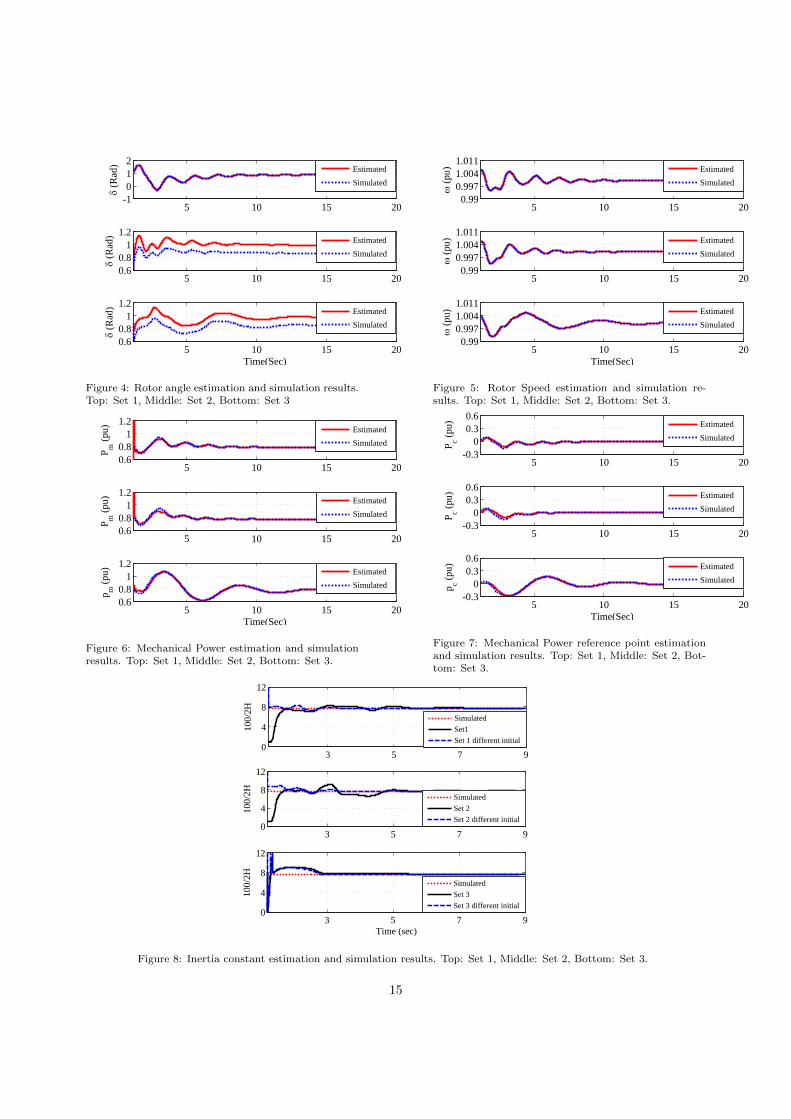
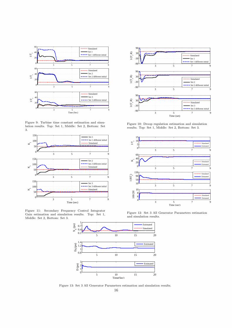
Figs. 4-7 present the estimation of states compared to the states from the simulation model. As it canbe seen, because the same classic generator model is used for both estimation and simulation model, therotor angle estimation matches the simulated rotor angle exactly for Set 1 scenario. In both Set 2 and Set 3,subtransient generator model is used in simulation while classic generator model is employed in estimation.Therefore, there is discrepancy between the rotor angles from the estimation and from the simulation,though the dynamic trends match each other well. Detailed discussion about such discrepancy can be foundin [11]. Figs. 8-11 show the estimation and simulation result for inertia constant, turbine-governor timeconstant, droop regulation and the secondary frequency control gain respectively. It is found that even fora complicated generator model equipped with PSS and AVR, UKF can estimate all parameters and statevariables with good accuracy.

Measurement Noises. In previous scenarios, the measurement errors were assumed to be normal distributionand very small (variance: 10−15). In order to show the effect of noise of normal distribution on the proposedmethod, three different simulation scenarios were carried out with adding 1%, 2% and 5% Gaussian noises tothe Set 3 of the recorded data. The estimation results are compared to the previous parameters estimation.Table 2 presents the results for those scenarios. As it would be expected, It can be seen from the table thatestimation error increases exponentially with increasing variance of the measurement noise. Although theerror of the estimation increases with respect to the increasing level of measurement noise, the results of theproposed method still shows acceptable accuracy for the most of its applications.

Model Validation. In the validation step, estimated parameters are used to build a low order generatordynamic simulation model as shown in Fig. 1. Then, event playback proposed in [4, 24] is used to validatethe estimation model. During event play back, hybrid dynamic simulation injects the inputs (measured PMUdata) to the low-order dynamic simulation model, output from the model will be captured and comparedwith the actual measurements.

In the previous sections, although UKF is used to estimate parameters, some parameters such as x′d andEq are assumed to be known. Moreover, all the generator model needs to have damping ratio to stabilizethe system. Therefore, in this section, UKF method is adjusted to estimate all the parameters of the model.In another word, transient reactance (x′d), generator internal voltage (Eq) and generator damping ratio (D)are added to the parameters which have to be estimated by UKF method. Thus, the augmented state vectorwill be Xk = [δk ωk Pmk

Pck Gk Jk Mk Kik x′dk Eqk Dk]T . The PMU data are presented in Fig. 3.Kalman filter’s parameter estimation are demonstrated in Figs. 12 and 13.

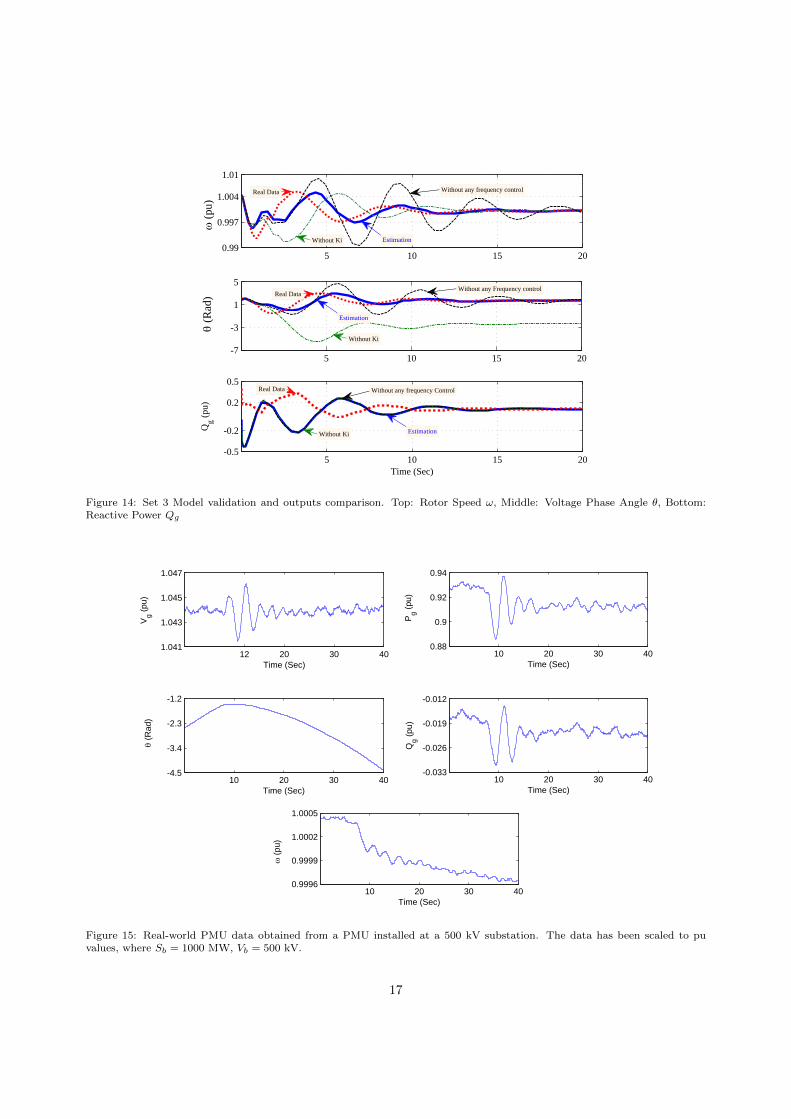
Estimated parameters have been used to build a continuous dynamic model of the generator in Mat-lab/Simulink. Then, input data (active power and voltage magnitude) are fed into the model to generateoutputs. Frequency, reactive power, along with voltage phase angle are compared with the data measure-ments. Fig. 14 shows the result of validation. Three sets of models are constructed, one with all parametersincluded, the second one without considering secondary frequency control (without Ki) and the third onewithout considering any frequency control system (without R and Tr). As demonstrated in Fig. 14, consid-ering the frequency control systems in the estimation model will greatly improve the match of the outputsand the PMU data.

4.2. Case Study Based on Real-World PMU Data

In this section, UKF method is applied on the PMU data from an anonymous busbar of the MISO systemto estimate parameters of a generator dynamic model. In the real world applications, the only data availableis limited to PMU measurements. Equivalent dynamic models are sought. Therefore, it can be anticipatedthat for the real-world application, all the parameters of the generator are unknown and have to be estimatedby the UKF method. The augmented state vector will beXk = [δk ωk Pmk

Pck Gk Jk Mk Kik x′dk Eqk Dk]T .The initial guess of the state variables X0 and its covariance matrix P0 as well as the covariance matrix forthe processing noise are listed in Table 3.

Fig. 15 shows the PMU data of 40 seconds. The set of data was recorded by PMUs after a generatortrip event. The data contain significant noises. Besides, PMUs save the data with a 30 Hz sampling rate.Data starting from 12 seconds to 40 seconds are used for estimation. Note in the figures follows, the starting

8

time is 12 seconds. Experiments show that 30 Hz sampling rate does not yield satisfactory performanceof UKF. This finding concurs with the findings documented in [15] that measurements interpolation isneeded to improve the performance of Kalman filters. Our experiments show that the real data have to beinterpolated to 100 Hz for the UKF method to converge. Figs. 16 and 17 present the estimation processes.Table 4 documents the final parameters estimation results.

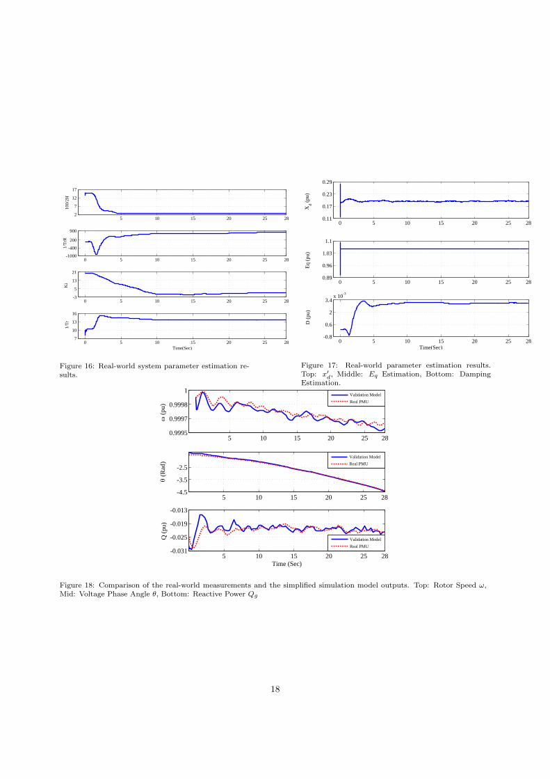
In the next step, the low-order model with estimated parameters was built in Matlab/Simulink. Eventplayback is used to inject voltage magnitude and active power as inputs. The outputs from the estimatedmodel and the output PMU measurements (frequency, voltage phase angle and reactive power) are compared.Fig. 18 shows the validation results. It is observed that despite the high level of noise and unknown dynamicsystem model structure, comparison of the PMU data with the validation model outputs shows a good degreeof match. The real-world PMU data case study demonstrates the feasibility of the proposed estimation modelin identifying a generator model.

5. Conclusion

UKF is implemented in this paper to estimate dynamic states and parameters of a low-order synchronousgenerator model with both primary and secondary frequency control systems. The proposed method usesvoltage magnitude and active power measurements as inputs, voltage angle, reactive power and frequencyas outputs. Inertia constant, damping coefficient, turbine-governor time constant, droop regulation as wellas secondary frequency control gain will all be estimated. Both simulation data and real-world PMU dataare used for case studies. In this research, various techniques are implemented to improve UKF algorithmfor the this application. The techniques include: (i) parameter conversion to increase parameter detectionsensitivity from the measurements; (ii) measurements interpolating to have a higher sampling rate to improveUKF convergence. In the validation step, a low-order dynamic simulation model is constructed with theestimated parameters. Input data are fed into the model to generate output data. The generated outputdata will then be compared with the outputs from the measurements.

The case studies demonstrate the feasibility of the proposed UKF estimation approach for system iden-tification using PMU data. Through the proposed estimation method, a complex generator model can beemulated using a low-order generator with frequency controls. The case study on the real-world PMU datademonstrates the capability of the proposed UKF on identifying an equivalent generator model.

Acknowledgement

This work was supported partially through DOE/MISO grant “System Identification using PMU Data.”The first author would like to acknowledge the help from Vahid Disfani and Javad Khazaei.

References

[1] P. Yang, Z. Tan, A. Wiesel, A. Nehora, Power system state estimation using pmus with imperfect synchronization, PowerSystems, IEEE Transactions on 28 (4) (2013) 4162–4172.

[2] K. Schneider, Z. Huang, B. Yang, M. Hauer, Y. Nieplocha, Dynamic state estimation utilizing high performance computingmethods, in: Power Systems Conference and Exposition, 2009. PSCE ’09. IEEE/PES, 2009, pp. 1–6.

[3] Z. Huang, P. Du, D. Kosterev, B. Yang, Application of extended kalman filter techniques for dynamic model parametercalibration, in: Power Energy Society General Meeting, 2009. PES ’09. IEEE, 2009, pp. 1–8.

[4] Z. Huang, D. Kosterev, R. Guttromson, T. Nguyen, Model validation with hybrid dynamic simulation, in: Power Engi-neering Society General Meeting, 2006. IEEE, 2006, pp. 1–6.

[5] Z. Huang, K. Schneider, J. Nieplocha, Feasibility studies of applying kalman filter techniques to power system dynamicstate estimation, in: Power Engineering Conference, 2007. IPEC 2007. International, 2007, pp. 376–382.

[6] K. Kalsi, Y. Sun, Z. Huang, P. Du, R. Diao, K. Anderson, Y. Li, B. Lee, Calibrating multi-machine power systemparameters with the extended kalman filter, in: Power and Energy Society General Meeting, 2011 IEEE, 2011, pp. 1–8.

[7] M. Burth, G. C. Verghese, M. Velez-Reyes, Subset selection for improved parameter estimation in on-line identification ofa synchronous generator, Power Systems, IEEE Transactions on 14 (1) (1999) 218–225.

[8] M. Karrari, O. Malik, Identification of physical parameters of a synchronous generator from online measurements, EnergyConversion, IEEE Transactions on 19 (2) (2004) 407–415.

9

[9] C. Lee, O. T. Tan, A weighted-least-squares parameter estimator for synchronous machines, Power Apparatus and Systems,IEEE Transactions on 96 (1) (1977) 97–101.

[10] Z. Huang, P. Du, D. Kosterev, S. Yang, Generator dynamic model validation and parameter calibration using phasormeasurements at the point of connection, Power Systems, IEEE Transactions on 28 (2) (2013) 1939–1949.

[11] L. Fan, Y. Wehbe, Extended kalman filtering based real-time dynamic state and parameter estimation using pmu data,Electric Power Systems Research 103 (2013) 168–177.

[12] E. Ghahremani, I. Kamwa, Dynamic state estimation in power system by applying the extended kalman filter withunknown inputs to phasor measurements, Power Systems, IEEE Transactions on 26 (4) (2011) 2556–2566.

[13] E. Ghahremani, I. Kamwa, Online state estimation of a synchronous generator using unscented kalman filter from phasormeasurements units, Energy Conversion, IEEE Transactions on 26 (4) (2011) 1099–1108.

[14] M. Ariff, B. Pal, A. Singh, Estimating dynamic model parameters for adaptive protection and control in power system,IEEE Trans. Power Syst. PP (99) (2014) 1–11.

[15] N. Zhou, D. Meng, Z. Huang, G. Welch, Dynamic state estimation of a synchronous machine using pmu data: A compar-ative study, Smart Grid, IEEE Transactions on PP (99) (2014) 1–1.

[16] S. S. Haykin, S. S. Haykin, S. S. Haykin, Kalman filtering and neural networks, Wiley Online Library, 2001.[17] S. Julier, The scaled unscented transformation, in: American Control Conference, 2002. Proceedings of the 2002, Vol. 6,

2002, pp. 4555–4559 vol.6.[18] J. J. Hyun, L. Hyung-Chul, Analysis of scaling parameters of the batch unscented transformation for precision orbit

determination using satellite laser ranging data, Journal of Astronomy and Space Sciences 28 (3) (2011) 183–192.[19] S. Julier, J. Uhlmann, H. Durrant-Whyte, A new approach for filtering nonlinear systems, in: American Control Confer-

ence, Proceedings of the 1995, Vol. 3, 1995, pp. 1628–1632 vol.3.[20] S. Julier, J. Uhlmann, H. Durrant-Whyte, A new method for the nonlinear transformation of means and covariances in

filters and estimators, Automatic Control, IEEE Transactions on 45 (3) (2000) 477–482.[21] S. J. Julier, J. K. Uhlmann, New extension of the kalman filter to nonlinear systems, in: AeroSense’97, International

Society for Optics and Photonics, 1997, pp. 182–193.[22] H. Jouni, S. Simo, Optimal filtering with kalman filters and smoothers. manual for matlab toolbox ekf/ukf, Helsinki

University of Technology, Department of Biomedical Engineering and Computational Science.[23] P. Kundur, N. J. Balu, M. G. Lauby, Power system stability and control, Vol. 7, McGraw-hill New York, 1994.[24] D. Kosterev, Hydro turbine-governor model validation in pacific northwest, Power Systems, IEEE Transactions on 19 (2)

(2004) 1144–1149.

Table of Tables

1. Initial values for Three Parameters Estimation for a generator with Primary frequency control.

2. Effect of measurement noise on parameter estimation.

3. Initial state variables and covariance matrices for real-world PMU Data.

4. Parameters Estimation for Real-world PMU Data.

5. Generator parameters in Simpower simulations.

Table 1: Initial values for Three Parameters Estimation for a generator with Primary frequency control

X0 All Sets P0 Set 1 Set 2 Set 3 Q All Sets

δ 0 P11 0.1 0.1 0.1 Q11 10−5

ω 1 P22 10−5 1e−5 10−5 Q22 10−11

Pm 0.8 P33 0.1 0.1 0.1 Q33 10−9

Pc 0 P44 10−5 1e−5 1e−5 Q44 10−9

G 1 P55 10−4 1e−4 80 Q55 10−4

J 10 P66 240 35 76 Q66 10−12

N 1 P77 6.3 3.4 10 Q77 10−6

Ki 10 P88 77 64 20 Q88 10−4

10

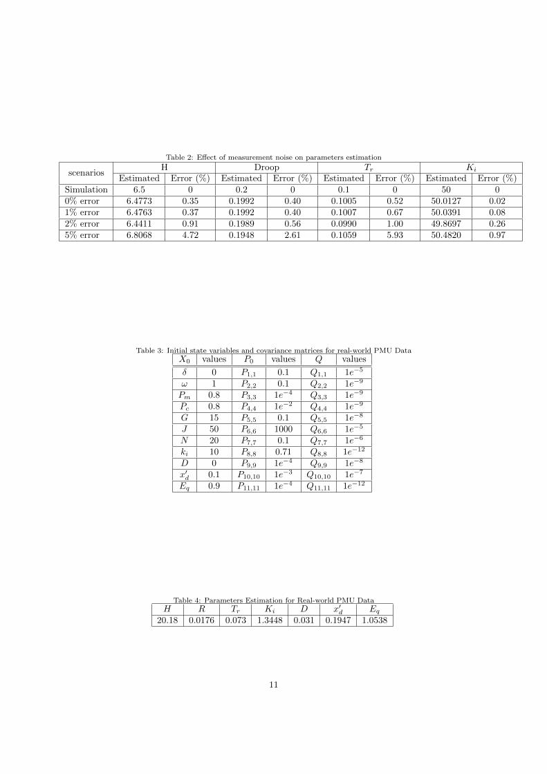
Table 2: Effect of measurement noise on parameters estimation

scenariosH Droop Tr Ki

Estimated Error (%) Estimated Error (%) Estimated Error (%) Estimated Error (%)Simulation 6.5 0 0.2 0 0.1 0 50 00% error 6.4773 0.35 0.1992 0.40 0.1005 0.52 50.0127 0.021% error 6.4763 0.37 0.1992 0.40 0.1007 0.67 50.0391 0.082% error 6.4411 0.91 0.1989 0.56 0.0990 1.00 49.8697 0.265% error 6.8068 4.72 0.1948 2.61 0.1059 5.93 50.4820 0.97

Table 3: Initial state variables and covariance matrices for real-world PMU DataX0 values P0 values Q values

δ 0 P1,1 0.1 Q1,1 1e−5

ω 1 P2,2 0.1 Q2,2 1e−9

Pm 0.8 P3,3 1e−4 Q3,3 1e−9

Pc 0.8 P4,4 1e−2 Q4,4 1e−9

G 15 P5,5 0.1 Q5,5 1e−8

J 50 P6,6 1000 Q6,6 1e−5

N 20 P7,7 0.1 Q7,7 1e−6

ki 10 P8,8 0.71 Q8,8 1e−12

D 0 P9,9 1e−4 Q9,9 1e−8

x′d 0.1 P10,10 1e−3 Q10,10 1e−7

Eq 0.9 P11,11 1e−4 Q11,11 1e−12

Table 4: Parameters Estimation for Real-world PMU DataH R Tr Ki D x′d Eq

20.18 0.0176 0.073 1.3448 0.031 0.1947 1.0538

11

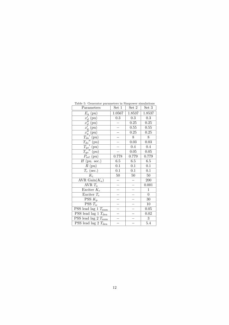
Table 5: Generator parameters in Simpower simulations

Parameters Set 1 Set 2 Set 3

Eq (pu) 1.0567 1.8537 1.8537x′d (pu) 0.3 0.3 0.3x′′d (pu) − 0.25 0.25x′q (pu) − 0.55 0.55

x′′q (pu) − 0.25 0.25

Tdo′ (pu) − 8 8

Tdo′′ (pu) − 0.03 0.03

Tqo′ (pu) − 0.4 0.4

Tqo′′ (pu) − 0.05 0.05

Pref (pu) 0.778 0.779 0.779H (pu. sec.) 6.5 6.5 6.5R (pu) 0.1 0.1 0.1Tr (sec.) 0.1 0.1 0.1Ki 50 50 50

AVR Gain(Ka) − − 200AVR Ta − − 0.001

Exciter Ke − − 1Exciter Te − − 0PSS Kp − − 30PSS Tw − − 10

PSS lead lag 1 Tnum − − 0.05PSS lead lag 1 Tden − − 0.02PSS lead lag 2 Tnum − − 3PSS lead lag 2 Tden − − 5.4

12

Table of Figures

1. Synchronous generator model including primary and secondary frequency controls.

2. The Study System.

3. Three sets of Matlab/SimPowerSystems simulation generated PMU measured data. Blue solid lines:Set 1; Read dashed lines: Set 2; Black dot-Dashed: Set 3.

4. Rotor angle estimation and simulation results. Top: Set 1, Middle: Set 2, Bottom: Set 3.

5. Rotor Speed estimation and simulation results. Top: Set 1, Middle: Set 2, Bottom: Set 3.

6. Mechanical Power estimation and simulation results. Top: Set 1, Middle: Set 2, Bottom: Set 3.

7. Mechanical Power reference point estimation and simulation results. Top: Set 1, Middle: Set 2,Bottom: Set 3.

8. Inertia constant estimation and simulation results. Top: Set 1, Middle: Set 2, Bottom: Set 3.

9. Turbine time constant estimation and simulation results. Top: Set 1, Middle: Set 2, Bottom: Set 3.

10. Droop regulation estimation and simulation results. Top: Set 1, Middle: Set 2, Bottom: Set 3.

11. Secondary Frequency Control Integrator Gain estimation and simulation results. Top: Set 1, Middle:Set 2, Bottom: Set 3.

12. Set 3 All Generator Parameters estimation and simulation results.

13. Set 3 All Generator Parameters estimation and simulation results (continued).

14. Set 3 Model validation and outputs comparison. Top: Rotor Speed ω, Middle: Voltage Phase Angleθ, Bottom: Reactive Power Qg.

15. Real-world PMU data obtained from a PMU installed at a 500 kV substation. The data has beenscaled to pu values, where Sb = 1000 MW, Vb = 500 kV.

16. Real-world system parameter estimation results.

17. Real-world parameter estimation results. Top: x′d, Middle: Eq Estimation, Bottom: Damping Esti-mation.

18. Comparison of the real-world measurements and the simplified simulation model outputs. Top: RotorSpeed ω, Mid: Voltage Phase Angle θ, Bottom: Reactive Power Qg.

AC/DC

AC/DC

DC/AC

AC/DC

DC/AC

DC/AC

S R

Cable SR

w1R

w2R

wnR

g1R

g2R

gmR

1 Terminal2 Terminal

n Terminal

1 Terminal

2 Terminal

m Terminal

T s +11

r 2 Hs + D1

R1

cP

gPmP Δω

ski

1sT

1

r 1Hs2

1

R

1

cP

LPmP Δω

refP

s1 Δ

s

1 ΔFigure 1: Synchronous generator model including primary and secondary frequency controls.

13

G1

1

G2

2

320

G3

11

G4

12

12013

101

Load 1 Load 2

Three Phase

Fault

Figure 2: The Study System.

5 10 15 200.99

1

1.01

Time (Sec)

(

pu)

5 10 15 200.4

0.8

1.2

Time (Sec)

P g (pu

)

5 10 15 20-0.2

0.1

0.4

Time (Sec)

Qg (

pu)

5 10 15 200.8

1

1.2

Time (Sec)

Vg (

pu)

5 10 15 20-0.5

0.5

1.5

Time (Sec)

(R

ad)

Figure 3: Three sets of Matlab/SimPowerSystems simulation generated PMU measured data. Blue solid lines: Set 1; Readdashed lines: Set 2; Black dot-Dashed: Set 3.

14

5 10 15 20-1012

(R

ad)

EstimatedSimulated

5 10 15 200.60.8

11.2

(R

ad)

EstimatedSimulated

5 10 15 200.60.8

11.2

Time(Sec)

(R

ad)

EstimatedSimulated

Figure 4: Rotor angle estimation and simulation results.Top: Set 1, Middle: Set 2, Bottom: Set 3

5 10 15 200.99

0.9971.0041.011

(p

u)

EstimatedSimulated

5 10 15 200.99

0.9971.0041.011

(p

u)

EstimatedSimulated

5 10 15 200.99

0.9971.0041.011

Time(Sec)

(p

u)

EstimatedSimulated

Figure 5: Rotor Speed estimation and simulation re-sults. Top: Set 1, Middle: Set 2, Bottom: Set 3.

5 10 15 200.60.8

11.2

P m (p

u)

EstimatedSimulated

5 10 15 200.60.8

11.2

P m (p

u)

EstimatedSimulated

5 10 15 200.60.8

11.2

Time(Sec)

p m (p

u)

EstimatedSimulated

Figure 6: Mechanical Power estimation and simulationresults. Top: Set 1, Middle: Set 2, Bottom: Set 3.

5 10 15 20-0.3

00.30.6

P c (pu)

EstimatedSimulated

5 10 15 20-0.3

00.30.6

P c (pu)

EstimatedSimulated

5 10 15 20-0.3

00.30.6

Time(Sec)

p c (pu)

EstimatedSimulated

Figure 7: Mechanical Power reference point estimationand simulation results. Top: Set 1, Middle: Set 2, Bot-tom: Set 3.

3 5 7 90

4

8

12

100/

2H

3 5 7 90

4

8

12

100/

2H

3 5 7 90

4

8

12

Time (sec)

100/

2H

Simulated

Set 3

Set 3 different initial

Simulated

Set 2

Set 2 different initial

Simulated

Set1

Set 1 different initial

Figure 8: Inertia constant estimation and simulation results. Top: Set 1, Middle: Set 2, Bottom: Set 3.

15

3 5 7 90

20

40

60

1/T

r

3 5 7 90

20

40

60

1/T

r

3 5 7 90

20

40

60

Time (Sec)

1/T

r

Simulated

Set 1

Set 1 different initial

Simulated

Set 2

Set 2 different initial

Simulated

Set 3

Set 3 different initial

Figure 9: Turbine time constant estimation and simu-lation results. Top: Set 1, Middle: Set 2, Bottom: Set3.

3 5 7 9-90

-30

30

90

1/(T

r.R)

3 5 7 9-90

-30

30

90

1/(T

r.R)

3 5 7 9-90

-30

30

90

Time (set)

1/(T

r.R)

Simulated

Set 1

Set 1 different initial

Simulated

Set 2

Set 2 different initial

Simulated

Set 3

Set 3 different initial

Figure 10: Droop regulation estimation and simulationresults. Top: Set 1, Middle: Set 2, Bottom: Set 3.

3 5 7 90

50

100

150

Ki

3 5 7 90

50

100

150

Ki

3 5 7 90

50

100

150

Time (sec)

Ki

Set 1

Set 1 different initial

Simulated

Set 2

Set 2 different initial

Simulated

Set 3

Set 3 different initial

Simulated

Figure 11: Secondary Frequency Control IntegratorGain estimation and simulation results. Top: Set 1,Middle: Set 2, Bottom: Set 3.

3 5 7 905

1015

1/T

r

3 5 7 90

20

40

60

Ki

3 5 7 910

50

90

130

1{R

Tr)

Simulated

Estimated

Simulated

Estimated

Simulated

Estimated

3 5 7 9468

10

Time (sec)

100/

2H

Simulated

Estimated

Figure 12: Set 3 All Generator Parameters estimationand simulation results.

5 10 15 200.10.40.7

1

Xd (p

u)

EstimatedSimulated

5 10 15 200.8

11.21.4

Eq (p

u)

5 10 15 200123

Time(Sec)

D (p

u)

Estimated

Estimated

Figure 13: Set 3 All Generator Parameters estimation and simulation results.

16

5 10 15 20-7

-3

1

5

(R

ad)

5 10 15 200.99

0.997

1.004

1.01

(

pu)

5 10 15 20-0.5

-0.2

0.2

0.5

Time (Sec)

Qg (

pu)

Without Ki

Without Ki

Estimation

Real Data

Estimation

Real Data

Real Data

Estimation

Without Ki

Without any frequency control

Without any Frequency control

Without any frequency Control

Figure 14: Set 3 Model validation and outputs comparison. Top: Rotor Speed ω, Middle: Voltage Phase Angle θ, Bottom:Reactive Power Qg

10 20 30 400.9996

0.9999

1.0002

1.0005

Time (Sec)

(p

u)

10 20 30 400.88

0.9

0.92

0.94

Time (Sec)

Pg (p

u)

10 20 30 40-0.033

-0.026

-0.019

-0.012

Time (Sec)

Qg (p

u)

12 20 30 401.041

1.043

1.045

1.047

Time (Sec)

Vg (p

u)

10 20 30 40-4.5

-3.4

-2.3

-1.2

Time (Sec)

(R

ad)

Figure 15: Real-world PMU data obtained from a PMU installed at a 500 kV substation. The data has been scaled to puvalues, where Sb = 1000 MW, Vb = 500 kV.

17

5 10 15 20 25 282

7

12

17

100/

2H

0 5 10 15 20 25 28-1000

-400

200

900

1/Tr

R

0 5 10 15 20 25 28-3

5

13

21

Ki

0 5 10 15 20 25 287

10

13

16

Time(Sec)

1/Tr

Figure 16: Real-world system parameter estimation re-sults.

0 5 10 15 20 25 280.11

0.17

0.23

0.29

Xd (p

u)

0 5 10 15 20 25 280.89

0.96

1.03

1.1

Eq (p

u)

0 5 10 15 20 25 28-0.8

0.6

2

3.4x 10-3

Time(Sec)

D (p

u)

Figure 17: Real-world parameter estimation results.Top: x′d, Middle: Eq Estimation, Bottom: DampingEstimation.

5 10 15 20 25 28-4.5

-3.5

-2.5

(R

ad)

5 10 15 20 25 280.9995

0.9997

0.9998

1

(

pu)

5 10 15 20 25 28-0.031

-0.025

-0.019

-0.013

Time (Sec)

Q (

pu)

Validation Model

Real PMU

Validation Model

Real PMU

Validation Model

Real PMU

Figure 18: Comparison of the real-world measurements and the simplified simulation model outputs. Top: Rotor Speed ω,Mid: Voltage Phase Angle θ, Bottom: Reactive Power Qg

18