ictiofauna del banco de galicia composición taxonómica y
TRANSCRIPT

Ictiofauna del Banco de Galicia
Composición taxonómica y aspectos
biogeográficos

ICTIOFAUNA DEL BANCO DE GALICIA: COMPOSICIÓN
TAXONÓMICA Y ASPECTOS BIOGEOGRÁFICOS
Autor: Rafael Bañón Díaz
TESIS DOCTORAL
Universidad de Vigo
Facultad de Ciencias del Mar
Departamento de Ecología y Biología Animal
VIGO 2016


Índice
- 1 -
ÍNDICE
1. Agradecimientos........................................................................................ 2
2. Motivación e Interés del estudio................................................................ 4
3. Objetivos.................................................................................................... 6
4. Resumen.................................................................................................... 7
5. Introducción General................................................................................. 16
5.1.- Área de estudio. El banco de Galicia como monte submarino.................. 17
5.2.- Antecedentes.............................................................................................. 20
5.2.1 Antecedentes en la explotación de los recursos......................................... 20
5.2.2 Antecedentes en la investigación científica............................................... 22
5.3.- Características oceanográficas................................................................... 24
5.4.- Marco geomorfológico del banco de Galicia............................................. 26
5.5.- Taxonomía íctica y nomenclatura.............................................................. 29
5.6.- Código de barras de ADN.......................................................................... 31
5.7.- Comentarios del doctorando...................................................................... 35
5.8.- Bibliografía................................................................................................ 37
6. Composición taxonómica y aspectos biogeográficos de la ictiofauna del
banco de Galicia........................................................................................
45
6.1.- Listado faunístico de la ictiofauna del banco de Galicia: especies
vulnerables y aspectos biogeográficos.......................................................
46
6.2.- Especies del género Apristurus (Elasmobranchii: Pentanchidae) en el
banco de Galicia........................................................................................
50
6.3.- Composición de especies de la familia Halosauridae
(Notacanthiformes) en el banco de Galicia...............................................
52
6.4.- Composición de especies y casos de hiperpigmentación en el género
Lepidion (Gadiformes: Moridae) en el banco de Galicia..........................
77
6.5.- Composición de especies de la familia Bathygadidae (Osteíctios:
Gadiformes) en el banco de Galicia...........................................................
81
6.6- Bibliografía................................................................................................ 83
7. Conclusiones.............................................................................................. 93
8. Anexos....................................................................................................... 95

Agradecimientos
- 2 -
1 AGRADECIMIENTOS
Agora de vello gaiteiro, no es fácil lanzarse a realizar una tesis doctoral a ciertas edades,
pero con un poco de entusiasmo, bastante de esfuerzo y algo de necesidad, hemos
logrado llegar al final del largo y tortuoso camino.
Mi primer agradecimiento va dirigido a la misma Mar, culpable de casi todo lo que
soy y sin la que no entendería la vida, y por añadidura a los mariñeiros, con los que
llevo compartiendo media vida en barcos y océanos polo mundo adiante (boa xente).
Gracias a mi familia, a mis padres y hermana, a Clara y Aldán (estudia vago), que me
aguantaron y sufrieron mis largas ausencias. En especial a mi padre, culpable de
meterme el gusanillo de la mar desde muy temprana edad.
Gracias a mis directores de tesis Alejandro y Alberto, sin cuyo apoyo y orientación
no sería posible su finalización.
Por suerte o por desgracia he recorrido numerosas instituciones y centros de
investigación y compartido diversión, trabajo, barcos y campañas de investigación con
numerosos compañeros y amigos. En el IIM-CSIC de Vigo realicé mis primeras
campañas al bacalao y la platija, y allí conocí y sigo conociendo a Antonio, Germán,
Fran, Rosa, Alex, David, Gonzalo, Jaime, Garci, Ángel, Marigel, Cristina, Eva, Iramaia,
Mima, Mariña, Sonia y Loli. Gracias a todos por vuestra amistad y ayuda y por el trato
exquisito que siempre me han dado en este centro, aún si pertenecer a él, un claro
ejemplo a seguir.
Mi siguiente paso fue por el Instituto Español de Oceanografía de Vigo, donde seguí
realizando campañas pesqueras a NAFO y Malvinas. Gracias a Carmen Gloria y Mikel,
compañeros en el proyecto de especies profundas, a Gersom, Isa, Itxaso, Neli,
Hortensia, Julio, José Luís, Pablo, Xulio, Ángeles, Lola ("hermana"), Esther, Conchi,
Lupe, Begoña, Valentín, Fernando (cabra, te quiero), María, Montse, Balta, Ana, Mima,
Santi y a todos los demás, gracias por todo.
Gracias al personal del Instituto Español de Oceanografía de Santander con los que
también compartí campañas, trabajo y alguna que otra fiesta. Gracias a Alberto,
Antonio, Fran, Enrique, Marián, Cristina, Paco, Olaya, Susana, Izaskun, Pablo, Jorge,
Agradecimientos
- 3 -
Isa y demás personal, gracias a todos. A Juan Carlos una dedicación especial por su
amistad, su ayuda y colaboración pasada presente y futura.
Gracias a la Consellería do Mar de la Xunta de Galicia, por permitirme hacer las
campañas de INDEMARES cuando aún estaba contratado con ellos y en especial a mis
ex compañeros de la UTPB, José Manuel, Alberto, Fernando, Jorge, Carmen, Manuel,
Luisa, Romi, Araceli y Bea, por todos los años pasados juntos.
Gracias a Sandra, David e Iago, del Departamento de Bioquímica, Genética e
Inmunología de la Universidad de Vigo, por su trabajo, aportaciones y enseñanzas en el
fascinante mundo de la taxonomía molecular.
Gracias a Jorge, Clara, Nieves, Belén, Auri, Antonio e Isa por vuestra amistad, las
cervezas, viajes y charlas compartidas.
Motivación e interés
- 4 -
2 MOTIVACIÓN E INTERÉS DEL ESTUDIO
La biodiversidad marina o diversidad biológica marina es el término que define la
variedad de seres vivos que habitan el medio marino. Los océanos, con una extensión de
361 millones de km2 (el 71% del planeta), son el lugar donde surgieron las primeras
especies animales hace 640 millones de años, representan un espacio para la vida 300
veces superior al del sistema terrestre y constituyen el hábitat de millones de especies.
Actualmente existen unas 275.000 especies de organismos marinos, pero se estima que
aún quedan por descubrir alrededor de 1.400.000. Cada año se descubren unas 1.600
nuevas especies y se calcula que se necesitarán entre 250 y mil años para inventariar
todas, con el riesgo que, para entonces, muchas puedan estar ya extinguidas.
Galicia presenta una alta biodiversidad biológica marina. Las condiciones
oceanográficas y biogeográficas, junto con la extraordinaria variedad de hábitats
costeros y oceánicos existentes configuran un medio marino muy complejo, con una
flora y fauna marinas enormemente diversas.
El número de especies marinas en Galicia está aún por determinar. En aguas de la
plataforma continental española se han descrito, hasta el momento, cerca de 1.000
especies vegetales y más de 7.500 animales. En cuanto a las especies de peces marinos,
los últimos estudios establecen en 954 las especies de la península y Baleares y más de
mil si sumamos las especies canarias.
Galicia cuenta con el ilustrado más destacado de la época en el ámbito de las ciencias
marinas, José Andrés Cornide y Saavedra (A Coruña, 1734-Madrid, 1803), quien puede
considerarse el padre de la ictiología en España. En 1788 publicó Ensayo de una
historia de los peces y otras producciones marinas de las costas de Galicia, arreglado
al sistema del caballero Linneo. En este trabajo se citan aproximadamente 65 especies,
que constituyen el primer listado de peces marinos de Galicia. Con el paso de los años y
las aportaciones de numerosos investigadores e instituciones, este número se ha
incrementado notablemente hasta las 398 especies inventariadas en el 2010. Sin
embargo, existe un claro desequilibrio entre el alto grado de conocimiento de la
ictiofauna litoral y de plataforma y el escaso conocimiento que se tiene de la ictiofauna
del talud, llanura abisal y montes submarinos.
Las profundidades marinas albergan uno de los mayores reservorios de la
biodiversidad marina, pero también constituyen uno de los ecosistemas más

Motivación e interés
- 5 -
desconocidos, debido a las dificultades y el reto tecnológico que supone su estudio. Sólo
los taludes continentales ocupan el 8,8 por ciento de la superficie mundial, frente al 7,5
por ciento de las plataformas continentales y los mares de aguas poco profundas. La
ictiofauna marina profunda de Galicia, entendida como aquella que habita
habitualmente a profundidades mayores de los 400 m, era escasamente conocida hasta
hace relativamente poco tiempo. En 1996 el Instituto Español de Oceanografía de Vigo
comienza un proyecto de prospección de especies comerciales en el talud de la
plataforma gallega. Los resultados de este proyecto dan lugar a un amplio listado de
especies, con aproximadamente 40 especies profundas nuevas para la ictiofauna gallega
e incluso española. La montaña submarina del banco de Galicia, con su cima a 625 m de
profundidad, constituye un hábitat profundo de características singulares. La elevada
profundidad, presencia de sustratos duros, fuertes pendientes, topografía críptica,
corrientes rápidas y variables, aguas oceánicas y aislamiento geográfico, hacen de los
montes submarinos un hábitat único para los organismos.
La ictiofauna que habita los montes submarinos ha desarrollado características
ecológicas y fisiológicas que les permiten explotar un ambiente de fuertes corrientes y
grandes flujos de materia orgánica. Presentan adaptaciones morfológicas al medio, una
longevidad alta, bajas tasas de crecimiento y reclutamientos altamente variables.
El banco de Galicia fue propuesto a la Comisión Europea como uno de los 10 nuevos
Lugares de Importancia Comunitaria (LIC), para incrementar la protección de nuestros
mares desde menos del 1% hasta más del 8%, en dirección al cumplimiento del
compromiso internacional del Convenio de Diversidad Biológica de proteger el 10% de
las regiones marinas del mundo.
Para proteger, primero es necesario conocer. Los estudios e investigaciones llevados
a cabo en esta tesis doctoral forman parte del proyecto LIFE+ INDEMARES que han
permitido finalmente la declaración del banco de Galicia como zona LIC (Decisión de
Ejecución (UE) 2015/2373 de la Comisión de 26 de noviembre de 2015 por la que se
adopta la novena lista actualizada de lugares de importancia comunitaria de la región
biogeográfica atlántica).

Objetivos
- 6 -
3 OBJETIVOS
El objetivo general de esta tesis es determinar la composición faunística de peces que
habitan el monte submarino del banco de Galicia y sus relaciones biogeográficas. Para
ello se han planteado cinco objetivos específicos.
1. Listar las especies identificadas en el banco de Galicia, determinar la
composición taxonómica y sus relaciones biogeográficas.
2. Determinar la composición de especies del género Apristurus (Pentanchidae) en
el banco de Galicia.
3. Determinar la composición de especies de la familia Halosauridae
(Notacanthiformes) en el banco de Galicia.
4. Determinar la composición de especies del género Lepidion (Moridae) en el
banco de Galicia, sus relaciones interespecíficas y la descripción de
hiperpigmentación melánica en ejemplares del género.
5. Determinar la composición de especies de la familia Bathygadidae (Gadiformes)
en el banco de Galicia.

Resumen
- 7 -
4 RESUMEN
La presente memoria doctoral viene a cubrir una parcela de conocimiento de la que se
tiene poca información en la actualidad, como es la composición de la ictiofauna que
habita los montes o montañas submarinas. El ser humano ha venido explorando y
explotando los mares desde tiempos ancestrales, primero las playas y costas someras
más cercanas, con el paso de los siglos, las amplias plataformas continentales y sólo
recientemente el talud continental y las montañas submarinas. Desde este punto de vista
cronológico, pues, las montañas submarinas, dada su inaccesibilidad y dificultades de
explotación, han permanecido desconocidas y en buen estado de conservación hasta la
actualidad, fuera de las fuertes presiones antrópicas costeras.
Un monte submarino es una elevación del fondo marino con una cumbre que no llega
a la superficie. Si bien no hay una definición particular que sea mayoritariamente
aceptada, una de las denominaciones más extendidas de monte submarino es aquella
que establece que desde su base tiene una altitud de al menos 1.000 metros y no alcanza
la superficie. Además de estas formaciones, existen otras miles de menor tamaño que
son catalogadas como colinas o montículos, dependiendo de sus dimensiones, y que
algunos autores consideran también que pueden desempeñar un papel importante en los
ecosistemas de aguas profundas y oceánicas.
El origen de estas formaciones es en su mayoría volcánico, pero existe un pequeño
porcentaje de origen continental. En este caso, las montañas submarinas surgen como
consecuencia de la fractura de los continentes o por la colisión o empuje de las placas
continentales.
El número estimado de montañas submarinos varía desde más de 100.000 mayores
de 1000 m hasta más de 25 millones si reducimos su altura hasta los 100 m. En el
océano Pacífico se contabilizan entre 30.000 y 50.000 montañas submarinas mayores de
1000 m, más de 800 en el océano Atlántico y un número indeterminado en el océano
Índico. En la zona del Convenio Oslo-París (OSPAR), hay 104 montañas submarinas
inventariadas, 74 dentro de la zona económica exclusiva nacional y sólo 30 fuera de
ella, en alta mar.
El banco de Galicia es un monte submarino de origen no volcánico localizado en el
margen continental de Galicia, a unos 200 km de la costa, en 42° 15′N y 43°N y 11°
30′W y 12° 15′W. El banco tiene una superficie de 1844 km2 en su parte más superficial

Resumen
- 8 -
y un contorno triangular, midiendo unos 75 km de largo por 58 km de ancho. Las
profundidades a las que se encuentra el techo del banco de Galicia varían entre 625 m,
en el sureste y 2000 m hacia el oeste.
El banco de Galicia es un monte submarino del tipo costero, perteneciente al grupo
situado a lo largo de las costas ibéricas y africanas de la Región IV (bancos de Galicia,
Ampere, Gorringe, Josephine y Seine), frente al grupo "offshore" del sur de Azores y
dorsal medio atlántica de la Región V (Atlantis, Hyeres, Irving, Meteor y Plato). En el
margen de Galicia se han identificado cinco plataformas marginales o montes
submarinos que forman relieves tabulares discontinuos en el ascenso continental: Porto,
Vigo, La Coruña, Finisterre y banco de Galicia.
El conocimiento de la existencia del banco de Galicia se remonta al año 1964, con la
publicación de un estudio geomorfológico de la zona. A nivel pesquero, los primeros
indicios de actividad tienen su origen a principio de la década de 1970, con varios
barcos de diversos puertos gallegos equipados con palangres o volantas que capturaban
primero especies demersales o bentopelágicas como la cherna (Polyprion americanus),
tomás (Epigonus telescopus) o alfonsino (Beryx splendens) y más tarde especies
epipelágicas como la palometa (Brama brama) y el pez espada (Xiphias gladius). La
actividad pesquera se ha ido reduciendo gradualmente con el tiempo y ya a partir del
año 2000 sólo algunos barcos faenaban de forma esporádica en la zona de estudio. La
baja y ocasional actividad pesquera realizada sobre el banco con artes de pesca
considerados poco destructivos (ausencia de arrastre) han permitido un alto grado de
conservación de este ecosistema.
El banco de Galicia está bañado por tres capas de diferentes masas de agua de origen
norteño y sureño: Masa de agua central del Atlántico NE europeo (East North Atlantic
Central Water: ENACW), por debajo de las aguas superficiales y hasta los 500-600 m;
Masa de agua mediterránea (Mediterranean Outflow Water: MOW) con dos núcleos
situados a 800 y 1200 m y Masa de agua del Labrador (Labrador Sea Water: LSW), que
tiene su centro sobre los 1800-1900 m. El relieve de las montañas submarinas interactúa
con la circulación oceánica circundante con la consiguiente formación de giros o anillos
("meddies"), corrientes circulares (columnas de Taylor) y afloramientos locales, que
causan incrementos locales de la producción primaria y secundaria por el ascenso de
nutrientes y fenómenos de retención y acumulación de larvas y plancton, modificando
las condiciones de oligotrofismo imperantes en el mar profundo.
Resumen
- 9 -
El margen continental del oeste de Galicia se clasifica como un margen continental
no volcánico, creado a partir de la propagación hacia el norte de la apertura del Océano
Atlántico, hace aproximadamente 110 millones de años. Presenta una geomorfología
formada por estructuras de bloques levantados y hundidos limitados por fallas normales
con dirección NNW-SSE que están cruzadas por fallas NE-SO. El origen del banco de
Galicia es probablemente tectónico, si bien ha sido modelado por los procesos
sedimentarios dominantes durante los descensos del nivel del mar. El banco presenta
pequeños relieves montañosos ("knolls"), crestas y canales, y dos valles rectilíneos de
40 m de relieve orientados en dirección NNW y que terminan abruptamente hacia las
850 m. La sedimentación en el flanco occidental del banco de Galicia posee la
singularidad de presentar rasgos detríticos de importancia regional forzados
climáticamente y asociados a procesos sedimentarios de talud continental.
Los peces, con unas 27.977 especies válidas, constituyen más de la mitad de especies
conocidas de vertebrados, en comparación con las 26.734 de tetrápodos. La
identificación de un ejemplar, consiste en adjudicarlo al grupo o taxón al que pertenece,
de acuerdo con un modelo clasificatorio elaborado anteriormente. En los peces, los
principales caracteres usados tradicionalmente para la identificación de especies son los
atributos descriptivos, las medidas morfométricas (biometrías) y los caracteres
merísticos. Existen, además, otros métodos utilizados más recientemente en la
identificación de peces. Entre ellos está la identificación taxonómica con marcadores
moleculares de ADN, que se ha ido instaurando con fuerza en los últimos años en la
taxonomía moderna. El código de barras de ADN (barcoding) utiliza como región
estándar la secuencia de una región de al menos 500 nucleótidos del extremo 5´ del gen
mitocondrial citocromo c oxidasa I (COI), y para cuya comparación se dispone tanto de
bases de datos de referencia (BOLD, Barcoding of life data) como generales
(GenBank).
La información recogida en esta memoria doctoral es el resultado de numerosas
campañas de investigación realizadas en el banco de Galicia desde 1980 hasta 2011,
tanto de carácter exploratorio, con barcos de pesca comercial, como de investigación
oceanográfico-pesquera, realizadas en buques oceanográficos. Aunque los objetivos y
metodología de ambos tipos de campañas difieren ligeramente, el objetivo final es muy
similar, conocer la composición de los organismos de la zona estudiada así como su
distribución y su abundancia.

Resumen
- 10 -
En el apartado 6.1 y anexo I de la presente memoria, se listan y comentan las 139
especies de 62 familias diferentes registradas en el banco de Galicia. La identificación y
clasificación de peces se hizo principalmente con la metodología clásica, examinando
los caracteres morfológicos descriptivos junto con las medidas biométricas y los
caracteres merísticos que delimitan cada especie. En especies cuya identificación
morfológica era más complicada o en aquellas en las que existe un interés taxonómico
especial por su rareza o falta de estudios, se realizó también una identificación
molecular con ayuda del código de barras de ADN.
De cada una de las especies listadas se aportan datos sobre su abundancia absoluta,
tallas y profundidad, así como de su hábitat, distribución y el grado de amenaza
existente sobre ella. Para algunas especies se aportan, además, los datos biométricos y
recuentos merísticos que permitieron su identificación.
Como consecuencia de las artes de pesca utilizadas y de su selectividad
interespecífica, la fauna bentopelágica es la mejor representada, si bien el listado recoge
especies de toda la columna de agua: epipelágicas, mesopelágicas, batipelágicas,
batidemersales y bentónicas. La familia mejor representada es Macrouridae, con nueve
especies, seguida por Moridae, Stomiidae y Sternoptychidae con siete cada una. Las
familias más abundantes son, Trachichthyidae y Moridae, debido a la gran cantidad de
ejemplares capturados de Hoplostethus mediterraneus (Trachichthyidae), con 61.206 y
de Lepidion lepidion (Moridae), con 41.585.
La mayor parte de las especies registradas son de aguas profundas, que viven
habitualmente a más de 400 m de profundidad. Por sus características biológicas y
ecológicas, los peces de las montañas submarinas son considerados como altamente
vulnerables. Estas especies presentan elevada longevidad, crecimiento lento, baja
fecundidad, madurez tardía y son muy vulnerables a las actividades humanas y cambios
naturales en el ecosistema.
El estado de vulnerabilidad y conservación de cada especie se caracterizó a partir de
dos listas globales (Unión Internacional para la Conservación de la Naturaleza, UICN y
FishBase) y una regional (OSPAR). Debido a los diferentes criterios utilizados para
estimar el estado de vulnerabilidad en cada lista, los resultados fueron muy diferentes.
Sólo cinco especies (3%) fueron consideradas como amenazadas según OSPAR, nueve
(6%) según UICN y 58 (42%) según FishBase. Este último es considerado el criterio
más apropiado, al ser un estudio con un gran número de especies y contener la lista de
UICN numerosas especies sin información. Del listado final hay que destacar el grupo

Resumen
- 11 -
de los elasmobranquios, con 31 especies, de las cuales 19 (61%) se encontrarían
amenazadas según FishBase.
Desde el punto de vista biogeográfico, el grupo de especies Atlánticas, que incluye
especies profundas o mesopelágicas de amplia distribución, con 113 especies (81%), es
el grupo más importante. Como consecuencia del carácter costero del banco de Galicia
también es notoria la ausencia de endemismos, de manera que la práctica totalidad de
especies registradas están presentes en aguas del Atlántico europeo.
Los resultados obtenidos en esta investigación muestran una elevada biodiversidad
piscícola y un alto porcentaje de especies amenazadas, lo cual apoya la reciente
declaración del banco Galicia como zona marina protegida.
En el apartado 6.2 y anexo II se identifican las especies del género Apristurus del
banco de Galicia. Este género es considerado como uno de los más diversos y
taxonómicamente confusos entre los elasmobranquios, debido a la gran cantidad de
especies poco conocidas y a su semejanza morfológica. Los ejemplares de Apristurus
fueron capturados en la campaña INDEMARES 2011, en los lances de mayor
profundidad, entre 1460 y 1809 m. Los individuos fueron identificados combinando
análisis morfológicos y moleculares. En total, fueron capturados 20 ejemplares, de los
cuales 18 resultaron ser Apristurus aphyodes, uno Apristurus melanoasper y otro
Apristurus profundorum. Esta última identificación constituye la cita más al norte
registrada para la especie en el Atlántico nororiental.
A nivel morfológico A. melanoasper se distingue de las otras dos especies por tener
el surco labial superior más largo que el inferior y un mayor número de válvulas
espirales en el intestino. Apristurus aphyodes se diferencia de A. profundorum por tener
un rostro ancho y corto (< 6% LT), y por una coloración más clara.
A nivel molecular, la identificación se realizó examinando el código de barras de
ADN del gen mitocondrial COI en A. profundorum y A. melanoasper y parte de la
secuencia del gen 16S rRNA en A. aphyodes, al no disponer de secuencias de COI de
esta especie en las bases de datos de referencia. Las secuencias obtenidas se agruparon
con las de referencia disponibles con un valor estadístico de remuestreo ("bootstrap")
del 99% para A. profundorum y A. aphyodes y del 95% para A. melanoasper,
confirmando las identificaciones morfológicas previas.
En el apartado 6.3 se determina la composición de especies de la familia
Halosauridae (Notacanthiformes) en el banco de Galicia. Se trata de una familia de
peces marinos que cuenta actualmente con 16 especies distribuidas en las aguas
Resumen
- 12 -
profundas y abisales de todo el planeta, entre 500 y 5000 m de profundidad, pero más
habitualmente entre 1100 y 3300 m. Los ejemplares fueron identificados combinando
análisis morfológicos y moleculares (código de barras de ADN).
Treinta y cinco ejemplares de seis especies de la familia Halosauridae fueron
capturados en dos localidades diferentes del norte de España entre los años 2009 y
2011, 33 en el banco de Galicia y dos en el banco El Cachucho, en el Golfo de Vizcaya.
En el primer sitio se identificaron 5 especies de 3 géneros distintos: Halosauropsis
macrochir, Halosaurus ovenii, Aldrovandia affinis, A. phalacra y A. oleosa mientras
que H. johnsonianus sólo apareció en el banco del Cachucho. Los registros de A. oleosa
en el banco de Galicia constituyen la primera cita de esta especie en aguas atlánticas
europeas y establecen un nuevo límite norte de distribución en el Atlántico este.
Morfológicamente, la ausencia de escamas en la parte superior de la cabeza distingue
los ejemplares de H. macrochir de los del género Halosaurus, y la presencia de escamas
en el hueso opercular los distingue del género Aldrovandia. Además, la distancia
interorbital en H. macrochir es mayor que en las especies de Halosaurus o Aldrovandia
(6.0-7.9 frente a 2.2-5.3% LGP). H. ovenii se diferencia de H. johnsonianus por tener
más escamas en la línea lateral hasta el ano (61-67 frente a 57), más ciegos pilóricos
(12-13 frente a 6-8) y menos branquiespinas en el primer arco branquial (12-13 frente a
17-18).
Entre las especies del género Aldrovandia, A. affinis se diferencia de A. phalacra y
A. oleosa por una mayor longitud preoral del rostro, contenida 2-2,2 veces en la
longitud del rostro (frente a 3-5,3) y menos branquiespinas en el primer arco branquial
(13-15 frente a 20-25). Aldrovandia phalacra difiere de A. oleosa por tener más
escamas en la línea lateral hasta el ano (26 frente a 20-22) y más radios en la aleta
pectoral (14-15 frente a 9-12).
A nivel molecular, las 35 secuencias de COI se agruparon en seis clados diferentes
que se correspondían con la asignación morfológica previa. Las diferencias existentes
en la secuencia de nucleótidos de los códigos de barras entre individuos se cuantificaron
en forma de distancia p o número de posiciones ocupadas por nucleótidos distintos en
relación con el total de posiciones examinadas. El valor porcentual medio obtenido
entre individuos de la misma especie fue 0,42% y entre individuos del mismo género
7,33%, un valor 17 veces superior. Además, el mayor valor de distancia obtenido entre
individuos de una especie fue 0,8%, mientras que al comparar individuos de distintas
especies del mismo género fue 3,3%, mostrando no sólo la ausencia de solapamiento
Resumen
- 13 -
entre ambas medidas sino la existencia de un número significativo de diferencias en
nucleótidos entre especie y género denominado "barcoding gap", que asegura la
aplicabilidad del procedimiento de utilización del código de barras de ADN a la
distinción de las especies que forman la familia Halosauridae.
En el apartado 6.4 y anexos III-1 y III-2 se estudian las especies del género Lepidion
(Moridae) del banco de Galicia y su relación con las demás especies del género.
Además, la hiperpigmentación melánica de un ejemplar de L. lepidion del banco
confirma la presencia de esta anomalía cromática en especies del género.
El género Lepidion Swainson, 1838 (Moridae), está compuesto por nueve especies
bentopelágicas que viven en el talud inferior y montes submarinos de los océanos
Atlántico, Índico, Pacífico y del Mar Mediterráneo. En el banco de Galicia se
identificaron dos especies, L. eques y L. guentheri. Para el estudio de las relaciones
entre especies y la comprobación de la eficacia del código de barras de ADN en la
identificación molecular de especies del género Lepidion, se obtuvieron 32 secuencias
de nucleótidos de COI de individuos pertenecientes a cinco especies diferentes de
Lepidion. Once de las secuencias procedían del banco de Galicia y el resto de diferentes
zonas del Golfo de Vizcaya y del Atlántico suroeste, a las que se sumaron 26 secuencias
de individuos del mismo género y diferentes especies procedentes de la base de datos
BOLD. Como resultado, se compararon 58 códigos de barras de ADN pertenecientes a
ocho de las nueve especies conocidas del género Lepidion. El alineamiento de las
secuencias y su posterior comparación, mediante inferencia bayesiana, produjo un árbol
consensuado en el cual las mismas se agruparon en siete clados distintos, con las
secuencias de dos especies, L. lepidion y L. eques, formando parte del mismo
agrupamiento, indicando una posible sinonimia. La distancia genética entre L. eques y
L. lepidion varió entre 0 y 0,62 % (con un valor medio de 0,29%) similar al valor de la
distancia media de todas las especies del género (0,27%) y muy por debajo del 2%
establecido de manera general como valor mínimo de distancia para discriminar
especies distintas. La distancia promedio entre pares de secuencias de distintas especies
fue de 4,28%, 16 veces mayor que la promediada entre individuos de la misma especie,
que fue de 0,27%. En este caso, las distancias entre secuencias se calcularon empleando
el modelo de sustitución de nucleótidos de Kimura 2 parámetros, si bien los valores
resultantes en el caso del gen COI, suelen ser similares a los que se obtienen calculando
las distancias p.

Resumen
- 14 -
A nivel morfológico, se analizaron comparativamente 36 ejemplares del Atlántico
identificados previamente como L. eques y 20 del Mediterráneo, identificados
previamente como L. lepidion. Los caracteres distintivos que separan a ambas especies
según la bibliografía son el diámetro del ojo, contenido entre 3,1 y 3,6 veces en la
cabeza en L. lepidion en vez de entre 2,6 y 3,1 veces en L. eques y el número de radios
de la aleta anal, entre 48 y 51 en L. lepidion frente a entre 50 y 54 en L. eques. Nuestros
resultados, sin embargo, muestran un gran solapamiento en los valores obtenidos de
estas variables entre ambas especies, lo que eliminaría su validez como carácter
taxonómico distintivo. El diámetro del ojo resultó estar contenido entre 2,8 y 3,6 veces
en la cabeza en L. lepidion y entre 2,6 y 3.4 veces en L. eques y el número de radios de
la anal fueron entre 45 y 51 en L. lepidion y entre 47 y 54 en L. eques. La biología de la
especie, con huevos y primeras fases de desarrollo pelágicas y las corrientes dominantes
tampoco sugieren barreras biogeográficas que interrumpan el flujo genético y delimiten
dos especies distintas.
Los resultados de los análisis morfológicos y moleculares junto con la información
biológica y oceanográfica sugieren que la especie endémica del Mediterráneo, L.
lepidion, y la especie del Atlántico norte, L. eques, son en realidad la misma especie,
por lo que L. eques es un sinónimo más moderno de L. lepidion.
En el apartado 6.4 y anexo III-2 se describen dos casos de hiperpigmentación
melánica o melanosis encontrada en dos ejemplares de L. lepidion (antes L. eques)
observados en el banco de Galicia y en el cañón de la Gaviera, en el Golfo de Vizcaya.
La pigmentación normal de L. lepidion es uniformemente pálida, variando de un color
pardo claro a un gris rosado, con las aletas algo más oscuras. Macroscópicamente, los
ejemplares con melanosis presentan una coloración atípica con la piel cubierta con
numerosas manchas oscuras e irregulares dispersas por la cabeza, el cuerpo y las aletas.
Microscópicamente, la histología muestra una hiperplasia de los melanóforos dérmicos
formando una capa gruesa y continua, paralela a la membrana basal. No se observaron
bacterias, parásitos u hongos que pudieran ser los causantes indirectos de esta
coloración. Sin embargo un trauma o herida fueron detectados tanto en el ejemplar de L.
lepidion del banco de Galicia como en otro de L. guentheri del Golfo de Vizcaya
publicado anteriormente, que podrían ser los desencadenantes originarios de la reacción
hiperplásica. El mismo patrón de coloración puede ser observado en la figura de un
ejemplar de L. lepidion del Mediterráneo que aparece en la publicación de Moreau en

Resumen
- 15 -
1881, siendo esta cita la primera documentación que se tiene de melanosis en el género
Lepidion y una de las primeras, si no la primera, en todos los peces.
En el apartado 6.5 y anexo IV, se analiza la composición de especies de la familia
Bathygadidae (Gadiformes) presentes en el banco de Galicia. Bathygadinae era
considerada tradicionalmente como una subfamilia de la familia Macrouridae, pero
recientes estudios basados en evidencias morfológicas y genéticas la han elevado al
rango de familia. Los batigádidos están ampliamente distribuidos, en zonas tropicales y
subtropicales de todos los océanos, entre 100 y 3000 m de profundidad. Entre 2009 y
2011, se capturaron nueve ejemplares de esta familia en el banco de Galicia y dos en el
cañón de Avilés. Los ejemplares fueron identificados combinando análisis morfológicos
y moleculares (código de barras de ADN).
Se identificaron cuatro especies de batigádidos, tres en el banco de Galicia (Gadomus
dispar, G. longifilis y Bathygadus melanobranchus) y una en el cañón de Avilés (G.
arcuatus) que representa un nuevo límite norte de distribución de la especie en el
Atlántico este. Morfológicamente, la ausencia de un barbillón en el extremo de la
mandíbula inferior y de radios muy alargados en las aletas diferencia las especies del
género Bathygadus de las del género Gadomus. Gadomus arcuatus tiene un número de
radios en la pectoral mayor que las otras especies de Gadomus (25 frente a 16–21).
Gadomus longifilis se diferencia de G. dispar por el número menor de radios en la aleta
pectoral (16–17 frente a 19–21), mayor número de branquiespinas en arco inferior del
primer arco branquial (29–31 frente a 19–21), mayor distancia interorbitaria (21,1–22.7
frente a 16,1–20.5 % longitud de la cabeza), menor longitud del barbillón (40,9–51,2
frente a 83,6–119,4 % longitud de la cabeza) y menor número de ciegos pilóricos (9–12
frente a más de 50).
A nivel molecular, las secuencias de nucleótidos correspondientes a los ejemplares
de la misma especie fueron idénticas entre sí, dando lugar a una única secuencia o
haplotipo representativo. La diversidad de nucleótidos global media encontrada al
comparar los códigos de barras (medida como distancia p) fue 9,6%. La de género fue
5,6% para Bathygadus y 8% para Gadomus. La distancia media entre los dos géneros
fue de 11,5%. La mayor divergencia encontrada ocurrió entre los haplotipos de B.
melanobranchus y G. arcuatus (12,4%) mientras que los valores menores se dieron
entre B. antrodes y B. favosus (5,1%).
Introducción general
- 16 -
5 INTRODUCCIÓN GENERAL

Introducción general
- 17 -
5.1 ÁREA DE ESTUDIO. EL BANCO DE GALICIA COMO MONTE
SUBMARINO.
El término montaña o monte submarino se ha definido de muchas y diferentes maneras,
pero no hay una definición particular que sea mayoritariamente aceptada. De manera
general, un monte submarino es una elevación del fondo marino con una cumbre que no
llega a la superficie. El origen geológico, la longitud vertical de la elevación y la forma
y tamaño de la cumbre van a ser las características principales que definen un monte
submarino según los distintos autores.
Una de las definiciones más extendidas de monte submarino lo describe como aquel
que tiene desde su base una altitud de al menos 1.000 metros y no alcanza la superficie
(Froese y Sampang, 2004; White y Mohn, 2004). Sin embargo, ninguna justificación
ecológica parece apoyar éste límite tradicional (Pitcher y col., 2007; Wessel, 2007) y
esta definición se ha modificado ampliamente en la bibliografía para satisfacer mejor las
necesidades de diferentes disciplinas. Algunos autores reducen la altitud mínima hasta
los 100 m (Staudigel y col., 2010; Morato y col., 2012) ya que los pequeños accidentes
submarinos también pueden desempeñar un papel importante en los ecosistemas de
aguas profundas y oceánicas (Koslow y col., 2001).
El origen de estas formaciones es en su mayoría volcánico (Wessel y col., 2010),
pero existe un pequeño porcentaje de origen continental, que surgen como consecuencia
de la fractura de los continentes o por la colisión o empuje de las placas continentales.
El número estimado de montes submarinos también varía, desde más de 100.000
mayores de 1000 m hasta más de 25 millones si reducimos su altura hasta los 100 m
(Wessel y col., 2010). En el océano Pacífico se contabilizan entre 30.000 y 50.000
montes submarinos mayores de 1000 m, más de 800 en el Océano Atlántico y un
número indeterminado en el Océano Índico (Rogers, 1994).
El número de montañas submarinas en el área OSPAR está aún sin calcular con
exactitud. Sin embargo, según Kitchingman y col. (2007) existen al menos 325 grandes
montañas submarinas, la mayor parte de ellas a lo largo de la dorsal atlántica y frente a
las costas de Portugal, España y Reino Unido. De las 104 montañas submarinas en la
base de datos de OSPAR, 74 se encuentran dentro de la zona económica exclusiva
nacional y sólo 30 fuera de ella, en alta mar (Serrao y col., 2010).
El banco de Galicia (BG) es un monte submarino del tipo costero, perteneciente al
grupo situado a lo largo de las costas ibéricas y africanas de la Región IV (BG, Ampere,

Introducción general
- 18 -
Gorringe, Josephine y Seine), frente al grupo offshore del sur de Azores y dorsal medio
atlántica de la Región V (Atlantis, Hyeres, Irving, Meteor y Plato) (Surugiu y col.,
2008). En el margen de Galicia se han identificado cinco plataformas marginales o
montañas submarinas que forman relieves tabulares discontinuos en el ascenso
continental: Porto, Vigo, La Coruña, Finisterre y BG (Vázquez y col., 2015).
Figura 1. Margen continental de Galicia, en el que se localizan el banco de Galicia (BG) y otros rasgos
geomorfológicos de la zona: los montes submarinos de Vasco da Gama (BVG), el banco de Vigo (BV), el
banco de Porto (BP), la cuenca interior de Galicia (CIG), la zona de transición (ZT), el flanco noroeste
(FNO), los montes Rucabado y García (BR), el margen profundo de Galicia (MPG), la llanura abisal de
Vizcaya (LLAV) y la llanura abisal ibérica (LLAI). Fuente: Proyecto ZEE (batimetría de ecosonda
multihaz) y Atlas Digital GEBCO.
El BG es un monte submarino profundo de origen no volcánico (Black y col., 1964)
situado al noroeste de la península ibérica, entre 42° 15′N y 43°N y 11° 30′W y 12°
15′W, a 120 millas náuticas de la costa noroeste española, en la Región noratlántica
(IXb2 del ICES), en la provincia biogeográfica Lusitánica de la Región IV de OSPAR
(Francia y Península Ibérica) (Fig. 1). Su origen está relacionado con el proceso de rift
continental Mesozoico que dio lugar a la apertura del océano Atlántico.
El BG (Fig. 2) tiene una superficie de 1844 km2 en su parte más somera, con un
contorno aproximadamente triangular, midiendo unos 75 km en dirección NNE-SSO,

Introducción general
- 19 -
por 58 km en dirección ONO-ESE (de la Torriente y col., 2014). Las profundidades a
las que se encuentra el techo del BG varían entre 625 m, hacia el sureste, y 2000 m,
hacia el oeste Hacia el este, el BG limita con una Zona de Transición que lo conecta con
la Cuenca Interior de Galicia, también conocida como surco de Valle Inclán, que capta
la mayoría de los sedimentos procedentes del continente. Hacia el norte y el noroeste, el
BG limita con los bancos submarinos de El Rucabado y García, que a su vez conectan
con un área de relieve escarpado, denominada Flanco Noroeste por Vázquez y col.
(2008). Este Flanco Noroeste o escarpe de Galicia, lleva a la Llanura Abisal de Vizcaya;
hacia el oeste y suroeste del BG, se encuentra el llamado Margen Profundo de Galicia
(Murillas y col., 1990), una zona de transición entre la corteza continental adelgazada y
la corteza oceánica de la llanura abisal ibérica.
Figura 2. Modelo digital del banco de Galicia y sus alrededores. Fuente: IEO
La parte superior del BG es relativamente plana, a excepción de la parte más oriental
que consiste en una serie de picos escarpados a lo largo de la vertiente oriental del
banco. La parte plana está cubierta por una gruesa capa de exudado de foraminíferos
planctónicos con un tamaño de grano medio de unas 190 micras y sólo el 0,2% de
carbono orgánico (Flach y col., 2002). La superficie del sedimento se compone de

Introducción general
- 20 -
numerosas pequeñas ondulaciones actuales y de "megaripples" ocasionales de unos 50
cm de altura, lo que indica movilidad y altas velocidades actuales de los sedimentos.
Comunidades de corales de aguas frías como Lophelia pertusa y Madrepora oculata
se encuentran en parches aislados cerca o encima de los "megaripples" (Somoza y col.,
2014). El pico oriental del banco consiste en roca basáltica estéril sin apenas corales u
otras formas de vida. La zona de transición entre la llanura de arena y las cumbres
áridas está densamente cubierta por crinoideos móviles (Duineveld y col., 2004). El
banco presenta también pequeños relieves montañosos ("knolls"), pequeñas crestas y
canales, y dos valles rectilíneos en el sector sur. Estos valles tienen 40 m de relieve,
están orientados en dirección NNO y su origen es probablemente tectónico, si bien han
sido modelados por los procesos sedimentarios dominantes durante los descensos del
nivel del mar (Black y col., 1964).
5.2 ANTECEDENTES
5.2.1 ANTECEDENTES EN LA EXPLOTACIÓN DE LOS RECURSOS
Existe poca información sobre la explotación de los recursos pesquero-marisqueros del
BG. Dada la lejanía del banco de los principales puertos pesqueros gallegos, la carencia
de cartas de la zona, las elevadas profundidades y el desconocimiento sobre la presencia
y abundancia de especies comerciales, es de suponer una actividad pesquera
relativamente reducida y reciente en el tiempo.
No se conoce con exactitud cuándo fue el primer momento que el sector pesquero
tuvo conciencia de la existencia del BG. La principal fuente de información proviene de
unos informes realizados sobre las primeras prospecciones de pesca promovidas por la
Asociación Provincial de Armadores de Pesca Fresca de Pontevedra, realizadas en el
banco con la ayuda científica del Instituto de Investigacións Mariñas (IIM-CSIC)
(Pérez-Gándaras, 1980), donde se nombran varios barcos de diversos puertos gallegos
con palangres o volantas. El primero de ellos, según dicho informe, fue el “Puerto de
Burela”, en 1971, con palangre de fondo. En 1975 se tiene constancia de la presencia de
dos volanteros, el “Sirín” y el “Rodriguez Baz”, con capturas de cherna (Polyprion
americanus), tomás (Epigonus telescopus), alfonsino (Beryx splendens) y brótola de
fango (Phycis blennoides). En 1979 se recoge la actividad de dos palangreros, el
“Nuevo Golondrina”, que capturó 140 cajas de palometa (Brama brama) y el “Monte
Real”, que hizo buenas capturas de pez espada (Xiphias gladius).
Introducción general
- 21 -
En 1980 ya había varios palangreros al pez espada, entre los que se nombran los
“Hermanos Bahamonde”, “Monte Real”, “Peña Liceira”, “Angel Mari” y “Playa de
Celeiro”, todos de la costa lucense. También se menciona algún intento de realizar
arrastre de fondo en la zona. A partir de 1985 hay entre cuatro y cinco barcos dirigidos a
la palometa roja (Beryx spp.), de tres a cuatro barcos que trabajan mediante la
modalidad de palangre de fondo y uno con la modalidad de enmalle (Serrano y col.,
2014). A final de la década de 1990 desaparece la pesquería de palangre de fondo
dirigida a Beryx spp, y es sustituida por la de enmalle dirigida a rape (Lophius spp). Al
mismo tiempo, comienza a desarrollarse una pesquería mediante palangre de fondo
dirigida a tiburones de profundidad, principalmente Centroscymnus coelolepis y
Centrophorus squamosus. En esta pesquería participan aproximadamente tres barcos, en
función del año y de la época. A principios del 2000, unos siete barcos faenan de forma
esporádica en la zona de estudio. Cuatro barcos dedicados a la modalidad de enmalle
(miños y volantas), cuya especie objetivo es el rape, y tres dedicados a la pesca de los
tiburones de profundidad mediante la modalidad de palangre de fondo. Existe también
cierta actividad estacional en la pesquería de cacea dirigida al bonito (Thunnus
alalunga) de manera casi específica.
Finalmente, la implementación en los últimos años de una legislación más restrictiva
sobre los períodos de pesca (descanso semanal), las prohibiciones de la pesca de
tiburones de profundidad (Reglamento Europeo 1262/2012) y del calado de las artes de
enmalle a más de 600 m han contribuido a limitar la actividad pesquera en esta zona.
A nivel marisquero, la abundancia de cangrejo real Chaceon affinis fue también
documentada en la misma serie de prospecciones (Pérez-Gándaras, 1980, 1981a,b). En
dichos informes se mencionan unos rendimientos de 1,63 individuos/nasa y unas
posibilidades de pesca para cuatro embarcaciones de 700 kg de cangrejo real por barco
y día. Al final de la década de 1980 se descubre también la abundancia de este recurso
en el talud de la plataforma gallega, entre 15 y 40 millas de la costa.
En 1990-1991, y durante distintos períodos, la por entonces denominada Consellería
de Pesca, Marisqueo y Acuicultura (Xunta de Galicia) promueve la realización de
campañas experimentales subvencionadas para la captura de cangrejo real. De todos los
barcos que participaron en las campañas, tan solo uno de ellos, el “Madre Modesta”
faenó en el BG entre 612-640 m (Ramonell y col., 1990). Las capturas declaradas por
este barco fueron de 2594 individuos en 220 nasas, con unos rendimientos de 11,8
individuos/nasa, supuestamente con nasas grandes del tipo “nasa fanequeira”.

Introducción general
- 22 -
Por lo visto anteriormente, podemos considerar la presión pesquera realizada sobre el
banco como baja, con una actividad esporádica con artes de pesca considerados poco
destructivos, principalmente enmalle y anzuelo, lo que ha permitido un alto grado de
conservación de este ecosistema.
5.2.2 ANTECEDENTES EN LA INVESTIGACIÓN CIENTÍFICA
El BG ha siso objeto de interés en diversos y variados campos científicos. La primera
referencia bibliográfica sobre la existencia del BG la encontramos en Black y col.
(1964). Las primeras investigaciones llevadas a cabo en este entorno están dirigidas a
estudios geomorfológicos de la corteza, en donde figuran por primera vez mapas
batimétricos más o menos detallados (Sibuet y col., 1978; Vanney y col., 1979).
Los primeros estudios malacológicos surgen a raíz de las capturas accidentales de
corales y gorgonias durante las primeras prospecciones pesqueras, sobre los cuales se
encontraron adheridos diversas especies de moluscos. En un primer informe sobre la
riqueza malacológica del banco (Rolán y Gándaras, 1980) se citan dos braquiópodos y
30 especies de moluscos gasterópodos y bivalvos. Este listado fue publicado
posteriormente con ligeros cambios (Rolán y Pedrosa, 1981).
Posteriores campañas e investigaciones han permitido el descubrimiento de
numerosas especies marinas, alguna de ellas nuevas para la ciencia. Algunos ejemplos
son el monoplacóforo Laevipilina rolani (Warén y Bouchet, 1990), los solenogastros
Urgorria compostelana (García-Alvarez y Salvini-Plawen, 2001), Hemimenia
cyclomyata, H. glandulosa, Neomenia oscari y N. simplex (Salvini-Plawen, 2006), los
crustáceos Uroptychus cartesi (Baba y Macpherson, 2012) y Petalophthalmus
papilloculatus (San Vicente y col., 2014), la esponja carnívora Chondrocladia
robertballardi (Cristobo y col., 2015) o el gasterópodo Aforia serranoi (Gofas y col.,
2014), constituyendo en su conjunto una muestra de la importante biodiversidad que
alberga el banco.
Las primeras investigaciones científico-pesqueras con objeto de evaluar la
composición y abundancia de especies de interés pesquero en el BG tienen lugar por
parte del ya mencionado IIM-CSIC en distintos períodos de 1980 y 1981. Los estudios
fueron realizados a bordo de barcos de pesca de distintas modalidades (arrastre,
palangre) y las especies más abundantes fueron el reloj mediterráneo (Hoplostethus
Introducción general
- 23 -
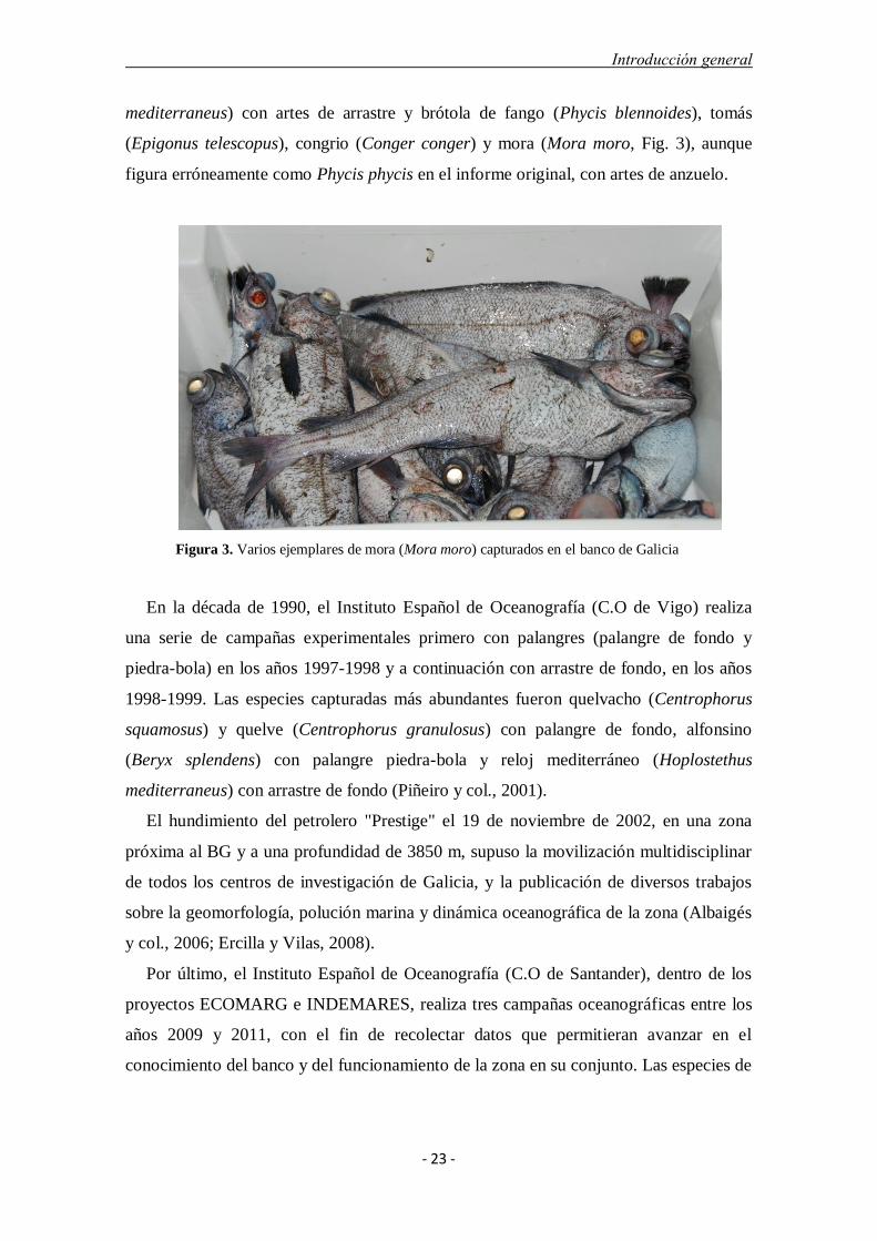
mediterraneus) con artes de arrastre y brótola de fango (Phycis blennoides), tomás
(Epigonus telescopus), congrio (Conger conger) y mora (Mora moro, Fig. 3), aunque
figura erróneamente como Phycis phycis en el informe original, con artes de anzuelo.
Figura 3. Varios ejemplares de mora (Mora moro) capturados en el banco de Galicia
En la década de 1990, el Instituto Español de Oceanografía (C.O de Vigo) realiza
una serie de campañas experimentales primero con palangres (palangre de fondo y
piedra-bola) en los años 1997-1998 y a continuación con arrastre de fondo, en los años
1998-1999. Las especies capturadas más abundantes fueron quelvacho (Centrophorus
squamosus) y quelve (Centrophorus granulosus) con palangre de fondo, alfonsino
(Beryx splendens) con palangre piedra-bola y reloj mediterráneo (Hoplostethus
mediterraneus) con arrastre de fondo (Piñeiro y col., 2001).
El hundimiento del petrolero "Prestige" el 19 de noviembre de 2002, en una zona
próxima al BG y a una profundidad de 3850 m, supuso la movilización multidisciplinar
de todos los centros de investigación de Galicia, y la publicación de diversos trabajos
sobre la geomorfología, polución marina y dinámica oceanográfica de la zona (Albaigés
y col., 2006; Ercilla y Vilas, 2008).
Por último, el Instituto Español de Oceanografía (C.O de Santander), dentro de los
proyectos ECOMARG e INDEMARES, realiza tres campañas oceanográficas entre los
años 2009 y 2011, con el fin de recolectar datos que permitieran avanzar en el
conocimiento del banco y del funcionamiento de la zona en su conjunto. Las especies de

Introducción general
- 24 -
peces recolectadas durante estas campañas van a constituir el material de partida de la
presente tesis doctoral.
5.3 CARACTERÍSTICAS OCEANOGRÁFICAS
El margen occidental de la península Ibérica se encuentra en el extremo nororiental del
giro subtropical. La circulación en este sector del Atlántico gira siguiendo el sentido de
las agujas del reloj, como resultado de la acción de los vientos alisios y vientos del
oeste, combinados con la fuerza de Coriolis, derivada de la acción de los márgenes
continentales.
El BG está bañado por capas de diferentes masas de agua de origen norteño y sureño.
Hasta tres masas de agua diferentes se pueden identificar en la zona (Cartes y col.,
2014; Somoza y col., 2014) (Fig. 4).
Masa de agua central del Atlántico NE europeo (East North Atlantic
Central Water: ENACW): por debajo de las aguas superficiales y hasta los
500-600 m. Formada por subducción y mezcla invernal en la región entre el
noreste de Azores y el margen occidental europeo (Pollard y Pu, 1985,
González-Pola y col., 2005). Dentro de estas aguas se pueden distinguir dos
subtipos de agua de origen y características termohalinas diferentes (Somoza y
col., 2014). El subtipo subtropical ENACWt (T=12,2‐18,5°C,
S=35,66‐36,75‰), cuyo origen se encuentra en un frente cerca de las Azores. El
subtipo subpolar ENACWp está formado por agua más fría y menos salina que
se forma en invierno en la parte este del Atlántico norte, sobre los 46°N, por
enfriamiento y convención profunda (T=4‐12°C y S=34,96‐35.66‰).
Masa de agua mediterránea (Mediterranean Outflow Water: MOW): se
forma en el Golfo de Cádiz a partir de la salida de agua profunda desde el mar
Mediterráneo al océano Atlántico a través del estrecho de Gibraltar y progresa
hacia el norte a lo largo del margen oeste ibérico. Esta agua relativamente densa,
a su salida de la cuenca mediterránea, comienza a mezclarse con agua más fría y
menos salina a medida que se desplaza, formando dos núcleos situados en 800 m
(AMs, T=13ºC, S=36.4‰) y 1200 m (AMs, T=13ºC, S=36.4‰) (Daniault y col.,
1994; Iorga y Lozier, 1999).

Introducción general
- 25 -
Masa de agua del Labrador (Labrador Sea Water: LSW): Capa más
profunda. Proviene del noroeste y tiene su centro sobre los 1800-1900 m
(Pingree, 1973; Johnson y col., 2005), con valores ya dados por Worthington y
Wright (1970) de T=2.4ºC y S=34.92‰.
Figura 4. Capas de agua que bañan el BG mostrando una sección vertical de salinidad a lo largo
de una sección meridional que cruza el eje principal del Banco en agosto de 2010 (izquierda) y
oxígeno disuelto (ml/l) a lo largo de una sección zonal que cruza el eje principal del banco. Se
muestran mapas con las isobatas de 1000 y 2000 m y las secciones (derecha). Proyecto
VACLAN/COVACLAN- IEO.
Por debajo de estas masas de agua, se reconocen otras masas de agua profunda que
no interactúan con la morfología del BG (Somoza y col., 2014).
El relieve de las montañas submarinas interactúa con la circulación oceánica
modificando las condiciones de oligotrofismo imperantes en el mar profundo. La
interrupción de las corrientes oceánicas, con la consiguiente formación de giros o
anillos ("meddies"), corrientes circulares (columnas de Taylor) y afloramientos locales,
son factores causantes de incrementos locales de la producción primaria y secundaria,
fundamentalmente por el ascenso de nutrientes y fenómenos de retención y acumulación
de larvas y plancton (Fock y col., 2002). La dinámica que se establece alrededor de los
montes submarinos es la de un sistema altamente complejo de interacciones que
depende de muchos procesos y características de éstos. La influencia de la estructura del
monte depende de diversas variables topográficas (altura y extensión), profundidad de la
cumbre, localización geográfica del monte (latitud y distancia a la plataforma
continental) y pendiente.
White y Mohn (2004) y Lavelle y Mohn (2010) resumen los procesos físicos
oceanográficos que se producen por la interacción entre las montañas submarinas y el

Introducción general
- 26 -
océano. En cuanto al BG, su impacto en la circulación en el Atlántico noreste ha sido
reconocido en distintos estudios (Mazé y col., 1997; Coelho y col., 2002; Colas, 2003).
Las columnas de Taylor, los "meddies", la marea interna o los filamentos de
afloramientos son algunos de estos fenómenos oceanográficos de mesoescala,
responsables de la enorme riqueza existente en el BG (Serrano y col., 2014). El cambio
de dirección de las corrientes marinas al chocar con el banco, producen las llamadas
columnas de Taylor, que tienen como consecuencia giros sobre la cima y finalmente un
enriquecimiento de las aguas que bañan el banco. La cima del banco está a una
profundidad de 625 m próxima a donde se localiza la vena de agua mediterránea. La
estratificación a esta profundidad favorece la intensificación de fenómenos como la
marea interna. Asimismo, al nivel de la capa de agua mediterránea, existe en el área
actividad de mesoescala, con vórtices conocidos como meddies. Estos meddies son
generados cerca de la costa y en su desplazamiento mar adentro pueden interaccionar
con el banco. Alvarez-Salgado y col. (2006) documentan una estructura ciclónica
observada sobre el banco causada probablemente por una rama de la Iberian Poleward
Current separada del talud en 42º N fluyendo al norte y oeste, que interactuaría con la
corriente de Portugal que fluye al sur y al este, rodeando el flanco occidental del banco.
De manera similar, la corriente mediterránea (MOW) se separa del talud, en
aproximadamente 42ºN, en dos ramas, una que fluye al oeste del BG y otra fluye hacia
el norte a lo largo del talud continental de la Península Ibérica (Mazé y col., 1997; Iorga
y Lozier, 1999).
Otro fenómeno de mesoescala que puede influir en el banco es la generación de
filamentos que exportan la producción del sistema de afloramiento hacia mar adentro y
pueden alcanzar el banco.
5.4 MARCO GEOMORFOLÓGICO DEL BANCO DE GALICIA
El margen continental del oeste de Galicia se clasifica como no volcánico, creado a
partir de la propagación hacia el norte de la apertura del océano Atlántico, hace
aproximadamente 110 M.a. (Malod y col., 1993). Presenta una geomorfología formada
por estructuras de bloques levantados y hundidos limitados por fallas. La región limita
al norte con la llanura abisal de Vizcaya y al oeste con la llanura abisal Ibérica.
En este margen continental se diferencian, de este a oeste, cinco unidades
fisiográficas (Fig. 5): (1) Plataforma continental, (2) Talud continental; (3) Cuenca

Introducción general
- 27 -
interior de Galicia, (4) Plataformas marginales y/o región de bancos submarinas, y (5)
Ascenso continental o margen profundo de Galicia.
Figura 5. Provincias fisiográficas del margen continental del noroeste de Iberia según Serrano y col.
(2014)
La plataforma continental es relativamente estrecha, con una anchura media de 35
km y su borde se sitúa a partir de 180-200 m de profundidad.
El talud continental presenta una anchura media de 22 km, con el límite inferior
sobre los 2.500‐3.000 m de profundidad. Está dividido en dos sectores, el talud superior,
hasta los 1800 m de profundidad, con pendientes relativamente altas, y el talud inferior,
hasta más allá de los 2500 m, con pendientes relativamente más suaves.
La cuenca interior de Galicia es una cuenca sedimentaria de grandes dimensiones
(350 km de largo, 100 km de ancho, 3-4 km de profundidad) que recorre el margen
oeste peninsular a partir de la plataforma continental gallega.
Las plataformas marginales y/o montañas submarinas forman relieves tabulares
discontinuos en el ascenso continental. De norte a sur son los siguientes: banco de
Galicia (~600 m de profundidad), Vigo (~2100 m de profundidad), Vasco da Gama
(~1750 m de profundidad) y Porto (~2200 m profundidad) (Pinheiro y col., 1996).
El Ascenso continental o Cuenca profunda de Galicia, se extiende desde 4000 a 5300
m de profundidad y está caracterizado por una topografía suave interrumpida por la
presencia de bancos geoestructurales.
En el marco geológico, el margen continental puede ser dividido en cinco áreas bien
delimitadas: (1) la plataforma continental; (2) la Cuenca Interior de Galicia; (3) los
Bancos Occidentales; (4) el Margen Profundo de Galicia y la Llanura Abisal de Iberia al

Introducción general
- 28 -
oeste; y (5) el Escarpe Septentrional de Galicia con la Llanura Abisal de Vizcaya al
norte.
La plataforma continental presenta una cobertura sedimentaria delgada y numerosos
afloramientos de rocas paleozoicas y mesozoicas. Se caracteriza por presentar una
textura mixta, tanto siliciclástica como carbonatada, con una banda longitudinal de
dirección N-S en la plataforma media compuesta por sedimentos limosos denominada
cinturón fangoso de Galicia (Ares y col., 2008).
La Cuenca interior de Galicia presenta un encuadre estructural formado por fallas
normales con dirección NNO-SSE cruzadas por fallas NE-SO (Boillot y col., 1988). El
basamento continental está fracturado por fallas normales y fallas afectando a bloques
estrechos (10-20 km) y alargados (60-100 km) basculados con dirección NE inclinadas
ligeramente al E (Alonso y col., 2008).
Los Bancos Occidentales que separan la Cuenca Interior de Galicia de la zona
profunda del margen se consideran como horsts tectónicos de la etapa extensional
mesozoica y reactivados posteriormente durante la etapa compresiva cenozoica (Boillot
y col., 1979).
El Margen gallego profundo se caracteriza por tratarse de un sistema sedimentario
profundo estructurado en bloques basculados por procesos de extensión que da lugar a
la formación de horsts, grabens y semigrabens.
El escarpe septentrional de Galicia constituye una zona compresiva cuyo basamento
pertenece al dominio oceánico.
El origen del BG es probablemente tectónico si bien ha sido modelado por los
procesos sedimentarios dominantes durante los descensos del nivel del mar (Black y
col., 1964).
La sedimentación en el BG no tiene un origen continental, sino que procede de la
propia columna de agua que cubre el monte submarino. Se trata, principalmente, de
sedimentos marinos que proceden fundamentalmente de restos de conchas de pequeños
organismos planctónicos y de otros depósitos procedentes de partículas removilizadas
que son depositadas en estas zonas por corrientes submarinas profundas (de la Torriente
y col., 2014).

Introducción general
- 29 -
5.5 TAXONOMÍA ÍCTICA Y NOMENCLATURA
Los peces constituyen más de la mitad del número total de las aproximadamente
54.711 especies conocidas de vertebrados. Hay descritas unas 27.977 especies válidas
de peces, en comparación con las 26.734 de tetrápodos (Nelson, 2006).
La sistemática es el estudio de las relaciones y la clasificación de los organismos, que
incluye las disciplinas de la nomenclatura y la taxonomía. La nomenclatura se ocupa de
asignar nombres científicos a los organismos y la taxonomía es la ciencia de la
descripción y la clasificación de los organismos, fundamental en la biología básica y
aplicada (Guerra-García y col., 2008).
Clasificar es organizar en grupos o conjuntos a distintos elementos u organismos que
comparten uno o más caracteres y que a su vez, pueden diferenciarse de los miembros
de otros grupos. Identificar un ejemplar consiste en adjudicarlo al grupo o taxón al que
pertenece, de acuerdo con un modelo clasificatorio elaborado con anterioridad (Lanteri
y col., 2004).
La correcta identificación de las especies ícticas es la base de otras disciplinas de la
biología básica como la ecología, biogeografía, biodiversidad, pero también de la
biología aplicada, como biología pesquera, salud animal y humana, fraude alimentario,
trazabilidad alimentaria, inspección pesquera, etc.
La taxonomía tradicional se basa en la descripción de los fenotipos (Boero, 2010), es
decir, de los caracteres morfológicos visibles que diferencian a una especie de otra. La
morfología es la disciplina de la zoología que estudia la forma, la estructura y el
desarrollo de los organismos (Lloris, 2015). Los caracteres morfológicos son las partes
observables o atributos de los organismos que constituyen la unidad del análisis
sistemático (Gill y Mooi, 2002).
En los peces, los principales caracteres usados tradicionalmente para la identificación
de especies son atributos descriptivos (Strauss y Bond, 1990), que hacen referencia a:
caracteres morfológicos distintivos (por ejemplo la forma del cuerpo, número y tipo de
radios de las aletas) (Fig. 6), medidas morfométricas (Fig. 7), que hacen referencia a
variables numéricas continuas (por ejemplo la longitud de la cabeza en relación a la
longitud del cuerpo) o caracteres merísticos, variaciones en el número de una estructura
o parte de ella, y que hacen referencia a variables numéricas discretas (por ejemplo el
número de radios blandos y espinosos de la aleta dorsal).

Introducción general
- 30 -
Cada especie tiene una serie de características bien definidas obtenidas a partir de un
primer espécimen utilizado para realizar la descripción taxonómica, llamado espécimen
tipo u holotipo. Los caracteres distintivos de varias especies constituyen una clave
dicotómica, que consiste en un modelo o esquema que permite la determinación de
distintas especies a través de la comparación de caracteres excluyentes (Lahitte y col.,
1997).
Figura 6. esquema básico de la anatomía de un pez mostrando las principales partes y estructuras de
carácter taxonómico. Fuente: Ichthyology at the Florida Museum of Natural History
(https://www.flmnh.ufl.edu)
Figura 7. Algunas de las principales biometrías utilizadas en la identificación de peces. Fuente:
Ichthyology at the Florida Museum of Natural History (https://www.flmnh.ufl.edu)
Introducción general
- 31 -
Además de la taxonomía clásica, basada principalmente en caracteres morfológicos
externos, actualmente se utilizan otros métodos en la identificación de peces. En una
reciente revisión, Fischer (2013) enumera hasta doce métodos distintos utilizados en la
identificación de organismos acuáticos. Algunos de ellos son derivados de la aplicación
de la taxonomía morfológica clásica, como por ejemplo la utilización de guías y claves
de identificación, la utilización de colecciones de referencia o sistemas integrados de
identificación online. Otros métodos son más novedosos, como IPez (Guisande y col.,
2010) que consiste en un sistema automático de identificación de peces basado en un
software de aprendizaje automático y que utiliza mediciones morfométricas de los
ejemplares. Las estructuras duras, como los otolitos, con una morfología característica
para cada especie, son utilizados en la identificación de peces teleósteos (Lombarte y
col., 2006), con especial utilidad en la identificación de presas de los contenidos
estomacales.
La identificación taxonómica con marcadores moleculares de ADN mitocondrial se
ha ido instaurando en los últimos años con mucha fuerza en la taxonomía moderna.
Teletchea (2009) enumera entre los más frecuentes citocromo b, 16S RNA, 12S RNA,
5S RNA, D-Loop, ATPasa, ATPasa 8, ND3/ND4 y COI. De todos ellos, citocromo c
oxidasa I (COI) es el que cuenta actualmente con más arraigo y aceptación.
5.6 CÓDIGO DE BARRAS DE ADN
En 2003, investigadores de la Universidad Guelph en Ontario (Canadá), animaron a
la comunidad científica implicada en el “Census of Marine Life” a la determinación de
códigos de barras de ADN de los especímenes que se iban recolectando. El análisis de la
secuencia de nucleótidos de un gen concreto previamente consensuado, con objeto de
permitir la identificación de la especie a la que pertenece, pasó a denominarse “DNA
barcoding” o examen de código de barras de ADN, por analogía con los códigos de
barras UPC (“universal product code”) de doce dígitos que sirven para la identificación
de mercancías (Hebert y col., 2003 a,b).
El fundamento de la identificación mediante código de barras de ADN estaría en el
hecho de que incluso una secuencia de ADN corta contiene información más que
suficiente como para distinguir diez o incluso 100 millones de especies. Por ejemplo, un
Introducción general
- 32 -
segmento de 600 nucleótidos perteneciente a un gen codificante de proteína contiene
200 posiciones correspondientes a la tercera base de cada codón. Al tratarse de un gen
proteico, en estas posiciones las sustituciones suelen ser neutrales desde el punto de
vista selectivo, y las mutaciones se acumulan por el proceso aleatorio de la deriva
génica. Incluso asumiendo que un grupo de organismos se encuentre sesgado al empleo
de AT o GC en las terceras posiciones de los codones, seguirá habiendo dos posibles
alternativas de base en 200 terceras posiciones distintas, es decir, 2200
= 1060
posibles
secuencias distintas basadas tan sólo en los cambios que ocurran en la tercera posición
de los codones. La prueba de que este principio es válido fue aportada mediante la
comparación de secuencias del gen mitocondrial codificante de la subunidad I del
enzima citocromo c oxidasa entre especies cercanas y entre diversos filos del reino
animal (Hebert y col., 2003b).
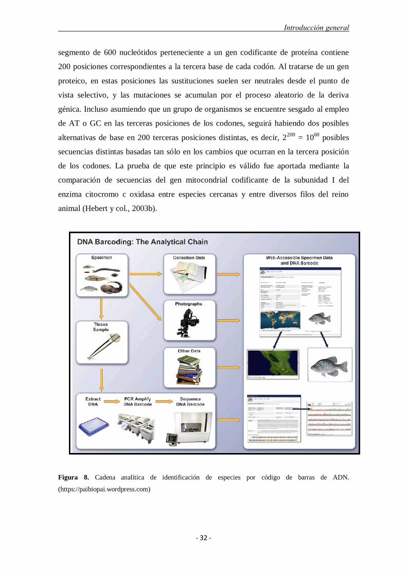
Figura 8. Cadena analítica de identificación de especies por código de barras de ADN.
(https://paibiopai.wordpress.com)

Introducción general
- 33 -
Ya en 2003 se especulaba con que el “DNA barcoding” tendría el potencial de ser un
método práctico para la identificación de los 10 millones de especies estimadas de
eucariotas sobre la tierra. Como método uniformizado de identificación de especies, el
examen del código de barras de ADN tendría amplias aplicaciones científicas, siendo de
gran utilidad en biología de la conservación, incluyendo campañas de estudio de la
biodiversidad. Podría ser incluso aplicado allí donde los métodos tradicionales no
consiguieran ser resolutivos como, por ejemplo, en la identificación de puestas,
embriones y formas inmaduras o en el análisis del contenido estomacal o de las
excreciones, para la determinación de cadenas tróficas. Además de la facilitación de la
identificación de especies, los códigos de barras de ADN ayudarían al análisis
filogenético y a revelar la historia evolutiva de la vida sobre la tierra.
Un gen apropiado cuya secuencia de nucleótidos pueda servir como código de barras
de ADN debe estar suficientemente conservado a lo largo del proceso evolutivo como
para que su amplificación, por PCR, pueda realizarse con cebadores de rango amplio y,
al mismo tiempo, debe divergir suficientemente como para permitir la discriminación
entre especies. Cierto número de genes podrían cumplir con los requisitos exigidos
(discriminación e identificación de especies, descubrimiento de especies nuevas y
crípticas, reconstrucción de relaciones evolutivas entre especies y taxones superiores).
La elección del gen mitocondrial codificantede la subunidad I del enzima citocromo c
oxidasa (COI) está apoyada por numerosos resultados experimentales (Achurra y
Erséus, 2013; Radulovici y col., 2010).
En algunos grupos taxonómicos, sin embargo, el código de barras de ADN no es
eficiente. Los cnidarios (anémonas, corales y algunas medusas), por ejemplo, exhiben
una diversidad de secuencia mitocondrial pequeña, tal vez por poseer un sistema
adicional de reparación de mutaciones del ADN mitocondrial. En las plantas superiores,
la secuencia de nucleótidos de COI es poco variable y, por lo tanto, no permite
identificar especies. Tampoco se resuelven bien, mediante examen del código de barras
de COI, las especies recién divergidas desde el punto de vista evolutivo y aquéllas
surgidas mediante hibridación.
Los puntos esenciales de la iniciativa de examen del código de barras son (Fig. 8):
1) preservación del espécimen en etanol al 95% para facilitar el aislamiento del
ADN.
2) amplificación y secuenciación del gen diana consensuado (COI).

Introducción general
- 34 -
3) depósito en una base de datos de las secuencias ligadas a los especímenes,
incluyendo datos adicionales de los mismos.
El éxito del examen de códigos de barras de ADN depende de la conexión entre la
secuencia de nucleótidos de COI a su correspondiente espécimen y sus datos asociados
(recolector, confirmación taxonómica, fecha, referencia geográfica en forma de
coordenadas, etc.).
Como secuencia de código de barras se utiliza el segmento 5´ del gen mitocondrial
que codifica la subunidad I del enzima de citocromo c oxidasa, que se abrevia como
COI-5P. Para su amplificación efectiva mediante reacción en cadena de la polimerasa
(PCR) existen un conjunto de cebadores de rango amplio válidos para peces (Ivanova y
cols., 2007).
Si bien inicialmente las secuencias de nucleótidos de código de barras de ADN
generadas por la iniciativa “Census of Marine Life” se depositaban en el banco de
secuencias generalista denominado GenBank (www.ncbi.nlm.nih.gov/genbank/), en la
actualidad se dispone de una base de datos específica de secuencias COI-5P,
denominada “Barcoding of Life Datasystems” (BOLD, www.boldsystems.org)
(Ratnasingham y Hebert, 2007), que incluye 24.000 registros de elasmobranquios y
237.004 de actinopterigios (22 de febrero de 2016).
La identificación de especies se basa en la divergencia de las secuencias de
nucleótidos COI-5 dentro y entre las especies (distancias intra e interespecificas).
Idealmente se espera la aparición de un "gap" o una zona donde el valor superior de las
distancias intra-específicas se encuentre alejado del valor inferior de las distancias inter-
específicas, de manera que no exista un solapamiento entre estos dos valores.
FISH-BOL, la campaña de código de barras de ADN de peces, es una colaboración
científica internacional que pretende crear una base de datos de referencia estandarizada
que incluya los códigos de barras de ADN de todos los peces (Ward y cols., 2009). El
análisis se dirige al examen de 648 pares de bases de la región 5´ del gen mitocondrial
citocromo c oxidasa I (COI). En 2009 se habían recogido más de 5.000 especies, con
una media de 5 códigos por especie, procedentes de sendos especímenes con
identificaciones realizadas por expertos (especímenes de referencia o “voucher”). Hasta
la fecha, los resultados indicaban que los códigos de barras separaban,
aproximadamente, el 98% de las especies de peces marinos examinadas. Mediante
taxonomía integrativa se pudo confirmar el estatus de especie nueva en el caso de varios
especímenes con secuencias de códigos divergentes inicialmente adscritos a la misma

Introducción general
- 35 -
especie. En relación con las precauciones debidas ante el uso de códigos de barras para
la discriminación entre especies, hay que decir que estas incluyen la hibridación, la
radiación evolutiva reciente, la diferenciación regional de los códigos y de copias
nucleares de los mismos. Los resultados indican que tales situaciones se han
contemplado escasamente en la inmensa mayoría de las especies estudiadas.
En peces, el valor medio de las diferencias en la secuencia de nucleótidos de códigos
de barras pertenecientes a ejemplares de la misma especie o distancia intraespecífica
media es de 0,3% (Zhang y Hanner, 2011), aproximadamente dos posiciones de
nucleótidos distintas en la secuencia del código de barras, y el límite para considerar
especies diferentes está cuando la variación sobrepasa el valor de 2% (Ward y col.,
2009). Sin embargo, no hay un patrón común para todas las especies y estos valores
pueden variar y no ajustarse a estas cifras. Por otro lado, Hebert y col. (2004) proponen
la "regla del 10x" como un indicador para la delimitación de especies, por el que dos
individuos se marcan como especies diferentes si sus secuencias de nucleótidos COI-5P
difieren al menos 10 veces más que la distancia intraespecífica media del grupo.
Finalmente, el depósito de las secuencias en bases de datos de referencia (por ejemplo
GenBank o Barcode of Life Data Systems, BOLD) va a permitir asignar con una alta
probabilidad de acierto secuencias de procedencia desconocida a secuencias de
organismos previamente descritos representadas por los especímenes “voucher”.
La aparición de una técnica de identificación molecular universal ha generado mucha
controversia sobre su validez y limitaciones (Ebach y Holdredge, 2005a,b; Ebach,
2011), pero su valor y eficacia sobre la morfología también han sido exaltados por otros
(Miller, 2007; Packer y col., 2009). Sin embargo, en los últimos años el concepto de una
taxonomía integrativa, no excluyente, se ha ido imponiendo (Dayrat, 2005; Kipling y
col., 2005; Goldstein y col., 2010). El código de barras de ADN no excluye a la
taxonomía clásica morfológica sino que la complementa y ambas son necesarias para la
correcta identificación de las especies.
5.7 COMENTARIOS DEL DOCTORANDO
Si bien esta tesis está centrada en la ictiofauna del BG, se han incluido especies del
mismo o similar nivel taxonómico capturadas fuera de esta área. La adicción de estas
especies fue considerada necesaria debido a su alto interés científico y a que pueden
servir como elementos comparativos y diferenciadores en la identificación de las

Introducción general
- 36 -
especies del BG, ya sea a nivel morfológico, pero sobre todo a nivel molecular, dada la
escasez de secuencias del gen COI de peces de aguas profundas depositadas en las bases
de datos de referencia, principalmente BOLD y GenBank. La exactitud de la
identificación molecular va a depender, entre otros factores, del número total de
secuencias que pertenecen a las especies identificadas y a taxones estrechamente
relacionados depositadas en las bases de datos (Millar y col., 2011).
Bibliografía
- 37 -
5.8 BIBLIOGRAFÍA
Achurra, A. & Erséus, C. 2013. DNA barcoding and species delimitation: the
Stylodrilus heringianus case (Annelida : Clitellata : Lumbriculidae). Invertebrate
Systematics, 27: 118–128.
Albaigés, J.B., Morales-Nin, B. & Vilas, F. 2006. The Prestige oil spill: A scientific
response. Marine Pollution Bulletin, 53: 205–207.
Alonso, B., Ercilla, G., Casas, D., Estrada, F., Farrán, M., García, M., Rey, D. & Rubio,
B. 2008. Late pleistocene and holocene sedimentary facies on the SW Galicia
Bank (Atlantic NW Iberian Peninsula). Marine Geology, 249: 46-63.
Álvarez–Salgado, X.A., Herrera, J.L, Gago, J., Otero, P., Soriano, J.A., Pola, C.G. &
García–Soto, C. 2006. Influence of the oceanographic conditions during spring
2003 for the transport of the Prestige tanker fuel oil to the Galician coast. Marine
Pollution Bulletin, 53: 239–249.
Ares, A., Rey, D., Rubio, B., Mohamed, K., Bernabeu, A. & Vilas, F. 2008.
Reconstrucción paleoclimática de la plataforma continental gallega basada en
datos geoquímicos y magnéticos. Geogaceta, 44: 87–90.
Baba, K. & Macpherson, E. 2012. A new squat lobster (Crustacea: Decapoda:
Anomura: Chirostylidae) from off NW Spain. Zootaxa, 3224: 49–56.
Black, M., Hill, M.N., Laughton, A.S. & Matthews, D.H. 1964. Three non-magnetic
seamounts off the Iberian coast. Quarterly Journal of the Geological Society of
London, 120: 477–513.
Boillot, G., Comas, M.C., Girardeau, J., Kornprobst, J., Loreau, J.-P., Malod, J.,
Mougenot, D. & Moullade, M. 1988. Preliminary results of the Galinaute cruise:
dives of the submersible Nautile on the Western Galicia margin, Spain. In:
Boillot, G., Winterer, E.L., et al., Publication Dates of ODP Proceedings.
Scientific Results, 103: College Station, TX (Ocean Drilling Program), pp: 37-
51.
Boero, F. 2010. The study of species in the era of biodiversity: A tale of stupidity.
Diversity, 2: 115–126.
Boillot, G., Auxietre, J.L., Dunand, J.P., Dupeuble, P.A., Mauffret, A. 1979. The
northwestern Iberian margin: a cretaceous passive margin deformed during the
Eocene. In: Talwani, M., Hay, W. & Ryan, W.B.F. (Eds.), Deep Drilling Results

Bibliografía
- 38 -
in the Atlantic Ocean: Continental Margins and Paleoenvironnement. Maurice
Ewing Series 3: Washington (Am. Geophys. Union), pp: 138–153.
Cartes, J.E., Papiol, V., Frutos, I., Macpherson, E., González-Pola, C., Punzón, A.,
Valeiras, X. & Serrano, A. 2014. Distribution and biogeographic trends of
decapod assemblages from Galicia Bank (NE Atlantic) at depths between 700
and 1800m, with connexions to regional water masses. Deep-Sea Research II,
106: 165–178.
Coelho, H.S., Neves, R.J.J., White, M., Leitao, P.C., Santos, A.J. 2002. A model for
ocean circulation on the Iberian coast. Journal of Marine Systems, 32: 153–179.
Colas, F. 2003. Circulation et dispersion lagrangiennes en Atlantique Nord-Est. Thèse
de Doctorat. Université de Bretagne Occidentale, Numéro de ordre 943.
Cristobo, J., Rios, P., Pomponi, S.A. & Xavier, J. 2015. A new carnivorous sponge,
Chondrocladia robertballardi sp. nov. (Porifera: Cladorhizidae) from two north-
east Atlantic seamounts. Journal of the Marine Biological Association of the
United Kingdom, 95: 1345–1352.
Dayrat, B. 2005. Towards Integrative Taxonomy. Biological Journal of the Linnean
Society, 85: 407415.
Daniault, N., Mazé, J.P. & Arhan, M. 1994. Circulation and mixing of Mediterranean
water west of the Iberian Peninsula. Deep Sea Research Part I, 41: 1685–1714.
de la Torriente, A., Serrano, A., Druet, M., Gómez-Ballesteros, M., Acosta, J., Parra, S.,
et al,. 2014. Banco de Galicia. Áreas de estudio del proyecto LIFE+
INDEMARES. Proyecto LIFE+ INDEMARES. Ed. Fundación Biodiversidad
del Ministerio de Agricultura, Alimentación y Medio Ambiente, 96 pp.
Duineveld G.C.A.,. Lavaleye, M.S.S & Berghuis, E.M. 2004. Particle flux and food
supply to a seamount coldwater coral community (Galicia Bank, NW Spain).
Marine Ecology Progress Series, 277: 13–23.
Ebach, M.C. & Holdredge, C. 2005a. DNA barcoding is no substitute for taxonomy.
Nature, 434: 697.
Ebach, M.C. & Holdrege, C. 2005b. More taxonomy, not DNA barcoding. BioScience,
55: 822–823.
Ebach M.C. 2011. Taxonomy and the DNA barcoding enterprise. Zootaxa, 2742: 67–
68.
Bibliografía
- 39 -
Ercilla, G. & Vilas, F. 2008. Geological characterization of the Galicia Bank Region
(Atlantic Ocean, NW Iberia): The marine geology community's response to the
Prestige disaster. Marine Geology, 249: 1–6.
Fischer, J. 2013. Fish identification tools for biodiversity and fisheries assessments:
review and guidance for decision-makers. FAO Fisheries and Aquaculture
Technical Paper No. 585, Rome, FAO, 107 pp.
Flach, E., Muthumbi, A. & Heip, C. 2002. Meiofauna and macrofauna community
structure in relation to sediment composition at the Iberian margin compared to
the Goban Spur (NE Atlantic). Progress in Oceanography, 52: 433–457.
Fock, H., Uiblein, F., Köster, F. & von Westernhagen, H. 2002. Biodiversity and
species–environment relationships of the demersal fish assemblage at the Great
Meteor Seamount (subtropical NE Atlantic), sampled by different trawls. Marine
Biology, 141: 185–199.
Froese, R. & Sampang, A. 2004. Taxonomy and biology of seamount fishes. In:
Morato, T. & Pauly, D. (Eds.), Seamounts: biodiversity and fisheries. Fisheries
Centre Research Reports 12, Vancouver, pp. 25–31.
García-Alvarez, O. & Salvini-Plawen, L.V. 2001. Urgorria compostelana gen. et sp.
nov. (Mollusca, Solenogastres, Rhopalomeniidae), a new species from off
Galicia, Northwest of Spain. Sarsia, 86: 183–189.
Gill, A.C. & Mooi, R.D. 2002. Phylogeny and systematics of fishes. In: P.J.B. Hart &
J.D. Reynolds (Eds.). Handbook of Fish Biology and Fisheries. Blackwell
Science, Oxford, pp. 15–42.
Gofas S., Kantor, Y. & Luque, Á. 2014. A new Aforia (Gastropoda: Conoidea:
Cochlespiridae) from Galicia Bank (NW Iberian Peninsula). Iberus, 32: 45–51.
Goldstein, P.Z. & DeSalle, R. 2010. Integrating DNA barcode data and taxonomic
practice: Determination, discovery, and description. Bioessays, 33: 135–147.
González-Pola, C., Lavín, A. & Vargas-Yánez, M. 2005. Intense warming and salinity
modification of intermediate water masses in the southeastern corner of the Bay
of Biscay for the period 1992–2003. Journal of Geophysical Research, 110:
C05020.
Guerra-García, J.M., Espinosa, F. & García-Gómez, J.C. 2008. Tendencias actuales en
Taxonomía: una visión sobre los principales temas de Taxonomía. Zoologica
baetica, 19: 15-49.

Bibliografía
- 40 -
Guisande, C., Patti, C., Patti, B., Mazzola, S., Jiménez, S., Duque-Nogal, V. Salmerón,
F., Manjarrés-Hernández, A., Pelayo-Villamil, P., Granado-Lorencio, C.,
Riveiro, I., Acuña, A., Prieto-Piraquive E. & Janeiro, E. 2010. IPez: An expert
system for the taxonomic identification of fishes based on machine learning
techniques. Fisheries Research, 102: 240–247.
Hebert, P.D.N., Cywinska, A., Ball, S.L. & DeWaard, J.R. 2003a. Biological
identifications through DNA barcodes. Proceedings of the Royal Society of
London B, 270: 313–321.
Hebert, P.D.N., Ratnasingham, S. & DeWaard J.R. 2003b. Barcoding animal life:
cytochrome c oxidase subunit 1 divergences among closely related species.
Proceedings of the Royal Society of London B, 270: S96–S99.
Hebert, P.D.N., Stoeckle, M.Y., Zemlak, T.S., Francis, C.M. 2004. Identification of
birds through DNA Barcodes. PLoS Biology, 2: 1657–1663.
Iorga, M.C. & Lozier, M.S. 1999. Signatures of the Mediterranean outflow from a
North Atlantic climatology 1. Salinity and density fields. Journal of Geophysical
Research, 104: 25985–26009.
Ivanova, N., Zemlak, T.S., Hanner, R.H. & Hebert, P.D.N. 2007. Universal primer
cocktails for fish DNA barcoding. Molecular Ecology Notes, 7: 544–548.
Johnson, G.C., Bullister, J.L. & Gruber, N. 2005. Labrador Sea Water property
variations in the northeastern Atlantic Ocean. Geophysical Research Letters, 32,
L07602: 1–5.
Kipling, W.W., Mishler, B.D. & Wheeler, Q.D. 2005. The perils of DNA barcoding and
the need for integrative taxonomy. Systematic Biology, 54: 844–851.
Kitchingman, A., Lai, S., Morato, T. & Pauly, D. 2007. How many seamounts are there
and where are they located? In: Pitcher, T.J., Morato, T., Hart, P.J.B., Clark,
M.R., Haggan, N. & Santos, R.S. (Eds.), Seamounts: Ecology, Fisheries and
Conservation. Fish and Aquatic Resources Series, Blackwell, Oxford, UK., pp:
26–40.
Koslow, J.A., Gowlett-Holmes, K., Lowry, J., O'Hara, T., Poore, G. & Williams, A.
2001. The seamount benthic macrofauna off southern Tasmania: community
structure and impacts of trawling. Marine Ecology Progress Series, 213: 111–
125.
Lahitte, H., Hurrell, J., Belgrano, M., Jankowski, L., Mehltreter, K., Haloua, P. &
Canda, G. 1997. Plantas de la Costa. Las plantas nativas y naturalizadas más

Bibliografía
- 41 -
comunes de las costas del Delta del Paraná, Isla Martín García y Ribera Platense.
Edición L.O.L.A. (Literature of Latin América), Buenos Aires, 200 pp.
Lanteri, A., Fernández, L. & Gallardo, F. 2004. Nomenclatura Biológica. In: Lanteri, A.
& Cigliano, M. (Eds), Sistemática Biológica: fundamentos teóricos y
ejercitaciones. EDULP, pp: 21–33.
Lavelle, J.W. & Mohn, C. 2010. Motion, commotion, and biophysical connections at
deep ocean seamounts. Oceanography, 23: 90–103.
Lloris, D. 2015. Paradojas y perplejidades de un taxónomo. In: Emilio Cervantes Ruiz
de la Torre (Ed.), Naturalistas en debate. Anejos Arbor, 9, pp: 67–90.
Lombarte, A., Chic, Ò., Parisi-Baradad, V., Olivella, R., Piera, J. & García-Ladona, E.
2006. A web-based environment from shape analysis of fish otoliths. The
AFORO database. Scientia Marina, 70: 147–152.
Malod J.A., Murillas, J., Kornprobst, J. & Boillot, G. 1993. Oceanic lithosphere at the
edge of a Cenozoic active continental margin northwestern slope of Galicia
Bank, Spain. Tectonophysics, 221: 195–206.
Mazé, J.P., Arhan, M. & Mercier, H. 1997. Volume budget of the eastern boundary
layer off the Iberian Peninsula. Deep Sea Research Part I, 44: 1543–1574.
Millar, C., Waugh, J. & Lambert, D.M. 2011. Are BOLD searches scientific? A
response to Federhen. 2011. Molecular Ecology Resources, 11: 939–940.
Miller, S.E. 2007. DNA barcoding and the renaissance of taxonomy. Proceedings of the
National Academy of Sciences, 104: 4775–4776.
Morato, T., Kvile, K. Ø., Taranto, G.H., Tempera, F., Narayanaswamy, B.E., Hebbeln,
D., Menezes, G., Wienberg, C., Santos, R.S. & Pitcher, T.J. 2012. Seamount
physiography and biology in North-East Atlantic and Mediterranean Sea.
Biogeosciences Discuss, 9: 18951–18992.
Murillas, J., Mougenot, D., Boillot, G., Comas, M.C., Banda, E. & Mauffret, A. 1990.
Structure and evolution of the Galicia interior basin (Atlantic western Iberian
continental margin). Tectonophysics, 184: 297–319.
Nelson, J.S. 2006. Fishes of the World, 4th edn. Hoboken, NJ:John Wiley & Sons, 601
pp.
Packer, L., Gibbs, J. Sheffield, C. & Hanner, R. 2009. DNA barcoding and the
mediocrity of morphology. Molecular Ecology Resources, 9: 42–50
Pérez-Gándaras, G. 1980. Informe sobre la campaña de prospección al banco de Galicia
(campañas de junio-julio y septiembre de 1980). IIM-CSIC, 46 pp.

Bibliografía
- 42 -
Pérez-Gándaras, G. 1981a. Informe sobre la campaña de arrastre en el banco de Galicia
(3ª campaña de prospección, Enero de 1981). IIM-CSIC, 23 pp.
Pérez-Gándaras, G. 1981b. Informe sobre una campaña de arrastre en el banco de
Galicia (4ª campaña de prospección, Octubre 1981). IIM-CSIC, 12 pp.
Pingree, R.D. & Morrison, G.K., 1973. The relationship between stability and source
waters for a section in the northeast Atlantic. Journal of Physical Oceanography,
3: 280–285.
Piñeiro, C.G., Casas, M. & Araújo, H. 2001. Results of exploratory deep-sea fishing
survey in the Galician Bank: Biological aspects on some of seamount-associated
Fish (ICES Division IXb). NAFO SCR Doc. 01/146 Serial No. N4540, 7 pp.
Pinheiro, L.M., Wilson, R.C.L., Pena dos Reis, R., Whitmarsh, R.B. & Ribeiro, A.
1996. The western Iberia margin: a geophysical and geological overview. In:
Whitmarsh, R.B., Sawyer, D.S., Klaus, A. & Masson, D.G. (Eds.), Proceedings
of the Ocean Drilling Program, Leg 149, Scientific Results Volume, pp: 3-23.
Pitcher, T.J., Morato, T., Hart, P.J.B., Clark, M.R., Haggan, R. & Santos, R.S. 2007.
The depths of ignorance: an ecosystem evaluation framework for seamount
ecology, fisheries and conservation. In: Pitcher, T.J., Morato, T., Hart, P.J.B.,
Clark, M.R., Haggan, N. & Santos, R.S. (Eds.), Seamounts: Ecology,
Conservation and Management. Fish and Aquatic Resources Series,
Blackwell, Oxford, UK.. pp: 476–488.
Pollard, R.T. & Pu, S. 1985. Structure and circulation of the upper Atlantic Ocean
northeast of the Azores. Progress in Oceanography, 14: 443–462.
Radulovici, A.E., Archambault, P. & Dufresne, F. 2010. DNA Barcodes for Marine
Biodiversity: Moving Fast Forward? Diversity, 2: 450–472.
Ramonell, R., Solórzano, M.R. & Romarís, X.M. 1990. Informe sobre la pesca del
cangrejo real en los meses de julio a octubre de 1990 en las costas de Galicia.
Xunta de Galicia, 7 pp.
Ratnasingham, S. & Hebert, P.D.N. 2007. BOLD: The barcode of life data system
(www.barcodinglife.org). Molecular Ecology Notes, 7: 355–364.
Rogers, A.D. 1994. The biology of seamounts. Advances in Marine Biology, 30: 305–
350.
Rolán, E. & Pérez-Gándaras, G. 1980. Moluscos recolectados en el Banco de Galicia.
IIM-CSIC, 7 pp.

Bibliografía
- 43 -
Rolán, E. & Pedrosa, G.P.G. 1981. Molluscs collected at the Galicia Bank (Spain). La
Conchiglia, 13: 6–10.
Salvini-Plawen, L.V. 2006. Five new Iberian Neomeniamorpha (Mollusca,
Solenogastres). Iberus, 24: 1–26.
San Vicente, C., Frutos, I. & Cartes, J.E. 2014. Petalophthalmus papilloculatus sp. nov.
(Crustacea: Mysida: Petalophthalmidae), a new bathyal suprabenthic mysid from
the Galicia Bank (NE Atlantic Ocean). Zootaxa, 3765: 77–91.
Serrano, A. et al. 2014. Informe final del proyecto LIFE+ INDEMARES
(LIFE07/NAT/E/000732), subproyecto LIC “Caracterización ecológica del
banco de Galicia”. Instituto Español de Oceanografía, Centro Oceanográfico de
Santander. Coordinación: Fundación Biodiversidad, Madrid, 237 pp.
Serrão, R., Tempera, F. & Morato, T. 2010. Background Document for Seamounts.
OSPAR Commission, 30 pp.
Sibuet, J.C., de Charpal, O., Montadert, L. & Ryan, W.B.F. 1978. Mouvements
verticaux dans la region des bancs de Galice (Atlantique nord-est) d'après les
résultats du leg 47 B. Bulletin de la Société géologique de France, 20: 365–373.
Somoza, L., Ercilla, G., Urgorri, V., León, R., Medialdea, T., Paredes, M., González,
F.J. & Nombela, M.A. 2014. Detection and mapping of cold-water coral
mounds and living Lophelia reefs in the Galicia Bank, Atlantic NW Iberia
margin. Marine Geology, 349: 73–90.
Staudigel, H., Koppers, A.A.P. Lavelle, J.W., Pitcher, T.J. & Shank, T.M. 2010. Box 1:
Defining the word "seamount". Oceanography, 3: 20–21.
Strauss R.E. & Bond, C.E. 1990. Taxonomic methods: morphology. In: Schreck C.B.
&, Moyle P.B. (Eds.), Methods for fish biology. American Fisheries Society,
Maryland, pp: 109–140.
Surugiu, V., Dauvin, J.C., Gillet, P. & Ruellet, T. 2008. Can seamounts provide a good
habitat for polychaete annelids?, Example of the northeastern Atlantic
seamounts. Deep Sea Research Part I, 55: 1515–1531.
Teletchea, F. 2009. Molecular identification methods of fish species: reassessment and
possible applications. Reviews in Fish Biology and Fisheries, 19: 265–293.
Vanney, J.R., Auxietre, J.L. & Dunand, J.P. 1979. North-western Iberian continental
margin geomorphology. Annales de l'Institut océanographique, 55: 5–20.
Vázquez, J.T., Medialdea, T., Ercilla, G., Somoza, L., Estrada, F., Fernández-Puga,
M.C., Gallart, J., Gràcia, E., Maestro, A. & Sayago, M. 2008. Cenozoic

Bibliografía
- 44 -
deformational structures on the Galicia Bank Region (NW Iberian continental
margin). Marine Geology, 249: 128–149.
Vázquez, J.T., Alonso, B., Fernández-Puga, M.C., Gómez-Ballesteros, M., Iglesias, J.,
Palomino, D., Roque, C., Ercilla, G. & Díaz-del-Río, V. 2015. Seamounts along
the Iberian Continental Margins. Boletín Geológico y Minero, 126: 483–514.
Ward, R.D., Hanner, R. & Hebert, P.D.N. 2009. The campaign to DNA barcode all
fishes, FISH-BOL. Journal of Fish Biology, 74: 329–3565.
Warén, A., & Bouchet, P. 1990. Laevipilina rolani, a new monoplacophoran from off
Southwestern Europe. Journal of Molluscan Studies, 56: 449–453.
White, M. & Mohn, C. 2004. Seamounts: a review of physical processes and their
influence on the seamount ecosystem. OASIS/National University of Ireland,
Galway, 38 pp.
Wessel, P. 2007. Seamount Characteristics. Chapter 1. In: Pitcher, T.J., Morato, T.,
Hart, P.J.B., Clark, M.R., Haggan, N. & Santos, R.S. (Eds.), Seamounts:
Ecology, Fisheries and Conservation. Fish and Aquatic Resources Series 12,
Blackwell, Oxford, UK, pp. 3–25.
Wessel, P., Sandwell, D.T. & Kim, S.S. 2010. The Global Seamount Census.
Oceanography, 23: 24–33.
Worthington, L.V. & Wright, W.R. 1970. North Atlantic Ocean atlas of potential
temperature and salinity in the deep water, including temperature, salinity and
oxygen profiles from the Erika Dan Cruise of 1962. Woods Hole oceanographic
Institution Atlas Series 2, 24 pp.
White, M. & C. Mohn. 2004. Seamounts: a review of physical processes and their
influence on the seamount ecosystem. OASIS/National University of Ireland,
Galway, 38 pp.
Zhang, J.-B. & Hanner, R. 2011. DNA barcoding is a useful tool for the identification of
marine fishes from Japan. Biochemical Systematics and Ecology, 39: 31–42.

Composición taxonómica
- 45 -
6 COMPOSICIÓN TAXONÓMICA Y ASPECTOS BIOGEOGRÁFICOS DE LA
ICTIOFAUNA DEL BANCO DE GALICIA

Composición taxonómica: listado
- 46 -
6.1 LISTADO FAUNÍSTICO DE LA ICTIOFAUNA DEL BANCO DE GALICIA:
ESPECIES VULNERABLES Y ASPECTOS BIOGEOGRÁFICOS
Comparados con el océano circundante, los montes submarinos son ecosistemas
altamente productivos y conocidos por su capacidad para soportar una gran
biodiversidad, incluyendo comunidades biológicas especiales como los arrecifes de
coral de aguas frías, abundantes recursos pesqueros, mamíferos, tortugas y aves marinas
(Niklitschek y col., 2010). Son, por tanto, hábitats de incalculable valor, tanto ecológico
como económico. Aunque la existencia de las montañas submarinas es conocida desde
hace cientos de años, la falta de tecnología para su exploración ha retrasado los estudios
biológicos exhaustivos hasta finales de 1950 (Hubbs, 1959). Aún hoy en día, con la
tecnología ya desarrollada, apenas unos 200 montes submarinos han sido estudiados en
profundidad (Secretariat of the Convention on Biological Diversity 2008), por lo que
todavía es muy escaso el conocimiento detallado de los hábitats, especies y su
distribución en estas montañas submarinas. El BG no es una excepción a esta regla
general; su descubrimiento para la ciencia es relativamente reciente (Black y col. 1964)
y los primeros estudios de los organismos que lo habitan datan de principios de 1980
(Rolán y Pedrosa, 1981).
La riqueza y diversidad ictiológica en las montañas submarinas no está bien
documentada (Fig. 9). Aunque el número de las montañas submarinas investigadas es
pequeño, cada vez es más evidente que las comunidades de peces que llevan asociadas
muestran adaptaciones específicas a estos hábitats y representan una porción
relativamente elevada y singular de la biodiversidad de peces (Morato y Clark 2007).
Koslow y col. (2000) describen las comunidades de peces de las montañas submarinas
como aquellas que tienen en común características morfológicas, ecológicas, biológicas
y fisiológicas que les permiten explotar con éxito un entorno con mayores corrientes y
flujo de materia orgánica que la mayoría de las profundidades marinas. Muchas especies
presentan adaptaciones a las fuertes corrientes al tener un cuerpo aplastado y presentan
además tasas metabólicas y de ingesta de alimentos relativamente altas.

Composición taxonómica: listado
- 47 -
Figura 9. Captura de un arte arrastre GOC en el banco de Galicia donde se puede observar en un primer
plano un ejemplar de Cataetyx laticeps.
Algunas especies demersales forman agregaciones en las montañas submarinas y
dada su abundancia y valor comercial son objeto de importantes pesquerías (Clark,
2009). Se han sugerido varias hipótesis sobre las grandes concentraciones de peces que
se producen alrededor de las montañas submarinas. Según Rogers (1994), el aumento de
las presas sobre las montañas submarinas es, a su vez, debido al aumento de la
producción primaria por los efectos topográficos y las condiciones hidrográficas locales
o por la migración diaria del plancton, que queda atrapados durante su descenso durante
el día por los depredadores que viven en la cima del monte submarino.
Pitcher (2010), cita las ocho especies con mayores capturas a nivel global en las
montañas submarinas: reloj anaranjado Hoplostethus atlanticus, alfonsino Beryx
splendens, tomás Epigonus telescopus, escolar Ruvettus pretiosus, sable negro
Aphanopus carbo, pez jabalí Pseudopentaceros richardsoni, granadero Coryphaenoides
armatus y reloj pardo sureño Pseudocyttus maculatus. En estos entornos se observan
también agregaciones de especies pelágicas, ya que funcionan como estaciones de
descanso, alimentación, reproducción y como puntos de orientación de muchas especies
pelágicas migratorias, entre las que figuran diversas especies de túnidos Thunnus spp.,

Composición taxonómica: listado
- 48 -
pez espada Xiphias gladius, marrajo Isurus oxyrinchus y marlín azul Makaira nigricans
(Morato y col., 2008, 2010).
Figura 10. El reloj mediterráneo Hoplostethus mediterraneus resultó ser la especie más abundante en el
banco de Galicia, muy frecuente en la zona más somera y sedimentaria (Fuente: IEO-INDEMARES).
En el monte submarino del BG se han identificado 139 especies de peces marinos
(ver anexo I). El listado se basa en nueve campañas de prospección e investigación
llevadas a cabo desde 1980 hasta 2011 con diferentes artes de pesca. Las especies se
agrupan en 2 superclases, 3 clases, 20 órdenes, 62 familias y 113 géneros. Las familias
más diversas son Macrouridae con 9 especies, seguida por Moridae, Stomiidae y
Sternoptychidae con 7 especies cada una. Por especies, el trachíchtido Hoplostethus
mediterraneus (Fig. 10) y el mórido Lepidion lepidion fueron las más abundantes.
Debido probablemente a la gran extensión del banco, las numerosas campañas
realizadas y los diferentes métodos de muestreo, el BG, es uno de los montes
submarinos de los que mejor se conoce su ictiofauna, en comparación con otros montes
submarinos del Atlántico Norte. Las 139 especies identificadas suponen una cifra muy
superior a las 40 especies de Gorringe (Abecasis y col., 2009), 78 especies de Sedlo
(Menezes y col., 2012), 53 especies de Meteor (Mohn, 2010) o las 34 especies de
Ampère (Christiansen y col., 2015), todos ellos situados en el entorno de las Azores.

Composición taxonómica: listado
- 49 -
A nivel biogeográfico, y teniendo en cuenta la totalidad de las especies de peces
presentes en el BG, 113 especies (81,3%) pertenecen al grupo Atlántico y 17 especies se
adscriben al grupo del Lusitánico (12,2%) (ver anexo I). Los resultados muestran una
ictiofauna compuesta en su mayor parte por especies de aguas profundas de amplia
distribución, similar a la del talud continental. La ausencia de especies endémicas en el
BG apoya la tesis que contempla los montes submarinos como ecosistemas singulares,
ricos en biodiversidad pero no aislados (Samadi y col. 2006; McClain, 2007).
Por sus características biológicas y ecológicas, los peces de los montes submarinos
son considerados como altamente vulnerables (Morato y col., 2006). En vista de las tres
bases de datos utilizadas para evaluar este criterio en el BG (OSPAR, UICN y
FishBase), 9 especies (6%) fueron consideradas como vulnerables según la UICN, 5
especies (3%) según OSPAR y 58 (42%) según FishBase. Sin embargo, en los casos de
datos no disponibles por la UICN o en estudios macro-ecológicos generales o con un
gran número de especies, el uso de las categorías de FishBase parece ser la mejor
opción (Strona y col. 2013). Por lo tanto, el 42% de las especies de peces registradas en
el BG, deben ser considerados como especies amenazadas (ver anexo I).
Los resultados obtenidos, una alta biodiversidad de peces y un alto nivel de
vulnerabilidad, apoyan la declaración del BG como Área Marina Protegida.

Composición taxonómica: Apristurus
- 50 -
6.2 ESPECIES DEL GÉNERO APRISTURUS (ELASMOBRANCHII:
PENTANCHIDAE) EN EL BANCO DE GALICIA
El género Apristurus (Garman, 1913) (Condríctios: Pentanchidae) constituye un grupo
de tiburones de aguas profundas de amplia distribución, con 37 especies reconocidas
hasta el momento (Froese y Pauly, 2016). Las especies de Apristurus se caracterizan por
tener un cuerpo largo y delgado, rostro largo y aplanado, aleta anal grande y elevada,
separada de la aleta caudal más baja por una escotadura y la ausencia de una cresta de
dentículos dérmicos en el margen superior de la aleta caudal en la mayoría especies
(Sato y col., 1999).
El género Apristurus estaba tradicionalmente incluido en la familia Scyliorhinidae,
pero recientes estudios filogenéticos moleculares y morfológicos han resucitado la
familia Pentanchidae, mostrando que la familia Scyliorhinidae era parafilética (Maisey,
1984; Winchell y col., 2004; Iglesias y col., 2005). Pentánchidos (es decir, géneros
Apristurus, Asymbolus, Bythaelurus, Cephalurus, Galeus, Halaelurus, Haploblepharus,
Holohalaelurus, Parmaturus y Pentanchus) difieren de esciliorhínidos sensu estricto (es
decir, géneros Atelomycterus, Aulohalaelurus, Cephaloscyllium, Poroderma,
Schroederichthys y Scyliorhinus) por la ausencia de las crestas supraorbitales en el
condrocráneo (Compagno, 1988). El género Apristurus comprende un grupo de
pintarrojas de aguas profundas y amplia distribución, que habitan los taludes
continentales y elevaciones submarinas a profundidades de 500 hasta 2100 m en todos
los océanos, excepto en aguas polares.
Figura 11. Vista dorsal de un ejemplar de Apristurus aphyodes Nakaya y Stehmann, 1998, especie de
Apristurus más frecuente en el banco de Galicia (Foto: Antonio Punzón).
Composición taxonómica: Apristurus
- 51 -
De las 89 especies de tiburones presentes en aguas europeas, 6 pertenecen al género
Apristurus (George y Zidowitz, 2006). En aguas españolas, sólo Apristurus laurussonii,
había sido descrita anteriormente, citada como A. atlanticus en las Islas Canarias
(Iglésias y Nakaya, 2004).
Varios ejemplares del género Apristurus fueron capturados en el monte submarino
del BG (NE Atlántico), entre 1460 y 1809 m profundidad, durante un estudio
multidisciplinario llevado a cabo en 2011 en el marco del proyecto INDEMARES (ver
anexo II). Los análisis morfométricos y moleculares permitieron la identificación de los
20 ejemplares capturados, de los cuales 18 fueron Apristurus aphyodes Nakaya y
Stehmann, 1998 (Fig. 11), uno A. profundorum (Goode y Bean, 1896) y otro A.
melanoasper Iglesias, Nakaya y Stehmann, 2004. Los resultados moleculares basados
en la comparación de códigos de barras de ADN apoyan la identificación de A.
profundorum y A. melanoasper, con valores estadísticos de re-muestreo del 99% y 95%,
respectivamente. La identificación molecular de A. aphyodes se realizó utilizando un
segmento de 499 nucleótidos del gen mitocondrial 16S. Estos son los primeros registros
de Apristurus en aguas gallegas, lo cual extiende su área de distribución conocida y
proporciona nueva información sobre diferentes aspectos biológicos y ecológicos de
este complejo grupo taxonómico.
Nakaya y Sato (1999), basándose en caracteres morfológicos como la longitud del
rostro, el número de válvulas espirales y la longitud de los surcos labiales, distinguen
tres grupos de especies diferentes en el género Apristurus (i.e. brunneus, longicephalus
y spongiceps). Más tarde, estos grupos fueron reconocidos como monofiléticos por
inferencias morfológicas y moleculares (Sato, 2000; Iglésias y col., 2005).
A. aphyodes y A. profundorum están incluidos en el grupo spongiceps, que se
caracteriza por tener entre 7 y 12 válvulas espirales en el intestino, el surco labial
superior subigual o más corto que el inferior y canal sensorial supraorbital continuo. A
melanoasper, sin embargo, está incluido en el grupo brunneus, que se caracteriza por
tener entre 12 y 23 válvulas espirales en el intestino, el surco labial superior más largo
que el inferior y canal sensorial supraorbital discontinuo.
El descubrimiento en el BG de 3 nuevas especies de Apristurus: A. aphyodes, A.
profundorum y A. melanoasper, incrementa notablemente el número de especies de este
género en aguas españolas y establece una nueva especie, A. profundorum, para aguas
europeas, como muestra de la importancia ecológica del banco y su aporte al
conocimiento de la biodiversidad ictiológica marina.
Composición taxonómica: Halosauridae
- 52 -
6.3 COMPOSICIÓN DE ESPECIES DE LA FAMILIA HALOSAURIDAE
(NOTACANTHIFORMES) EN EL BANCO DE GALICIA
Introducción
Notacanthiformes Goodrich 1909, es un orden de peces de aguas profundas que
contiene las familias Halosauridae (halosáuridos) y Notacanthidae (notacántidos o
anguilas espinosas) (Zhang, 2011). Los peces notacantiformes se caracterizan por tener
un cuerpo anguiliforme, rostro que sobresale visiblemente por delante de la boca,
grandes nódulos de tejido conectivo insertados entre el arco pterigoideo y el maxilar, y
aletas ventrales unidas en la línea media ventral del cuerpo (McDowell, 1973; Nelson,
2006; Wiley y Johnson, 2010).
Los halosáuridos son peces bentónicos o bentopelágicos que se encuentran en todos
los océanos, desde el talud de la plataforma continental hasta las llanuras abisales y
desde 500 hasta 5000 m de profundidad, pero más frecuentemente entre 1100 y 3300 m
(Klimpel y col., 2008). Aunque raramente son capturados, probablemente sean
frecuentes desde el talud inferior hasta las zonas abisales (Mceachran y Fechhelm,
1998). De hecho, Halosauropsis macrochir es una specie abundante en la dorsal
Atlántica (Klimpel y col., 2008).
La familia Halosauridae contiene actualmente 16 especies distribuidas por todos los
océanos y agrupadas en tres géneros: Halosaurus Johnson, 1863; Halosauropsis Collett,
1896 y Aldrovandia Goode & Bean, 1896 (Kamikawa y Stevenson, 2010; Eschmeyer,
2015). Su composición y distribución ha sido estudiada por diversos ictiólogos en
diferentes áreas: Atlántico Centro-Occidental (Smith, 2003); Atlántico Noroccidental
(McDowell, 1973); Atlántico Nororiental y mar Mediterráneo (Sulak, 1986a); sur de
África (Sulak, 1986b); Pacífico centro-occidental (Smith, 1999); Australia (Williams y
col., 1996) y mares del Sur (Gon, 1990).
En el Atlántico europeo, los halosáuridos están representados por cinco especies
(Sulak, 1986a; Alcázar y col., 1992; Quéro y col., 2003): Halosaurus johnsonianus
Vaillant 1888, Halosaurus ovenii Johnson 1864, H. macrochir (Günther, 1878),
Aldrovandia phalacra (Vaillant, 1888) y Aldrovandia affinis (Günther, 1877).
Las diferencias existentes entre secuencias del gen mitocondrial COI de distintas
especies pueden utilizarse como código de barras para facilitar la identificación de

Composición taxonómica: Halosauridae
- 53 -
especies, poner de manifiesto casos de expansión de especies conocidas, detectar
especies previamente omitidas y permitir identificaciones allí donde los métodos
tradicionales no pueden aplicarse (Hebert y col., 2003). El análisis se centra en una
región de aproximadamente 650 pares de bases de una región del extremo 5´de este gen.
Los beneficios resultantes de la simplificación de la identificación de especies se han
probado de manera extensiva en peces marinos, para los que los códigos de barras han
discriminado cerca del 98% de las especies previamente descritas (Ward y col., 2009).
Pueden darse excepciones entre especies que han divergido recientemente o entre
aquéllas que hibridan con regularidad. De manera alternativa, pequeñas diferencias
entre los códigos de barras de especímenes atribuidos a distintas especies pueden indicar
sinonimia, es decir, miembros de una única especie separados en taxones distintos, o
especímenes mal identificados (Ward y col., 2009). El examen de códigos de barras de
ADN se reconoce como una herramienta importante que puede ser aprovechada en la
resolución de cuestiones taxonómicas en peces (Ward y col., 2005, 2009; Zemlak y col.,
2009), basándose en el desarrollo de una base de datos de códigos de barras preparada a
partir de especímenes de referencia identificados fehacientemente por taxónomos
expertos (Federhen, 2011).
Material y Métodos
Recolección de muestras, identificación de especies y análisis morfológico
Los especímenes se capturaron en el transcurso de varias campañas oceanográficas
realizadas entre 2009 y 2011 con objeto de investigar la estructura de las comunidades
de profundidad en dos áreas de la costa española: el banco de Galicia y el banco El
Cachucho (noreste del Océano Atlántico).
Todas las muestras fueron identificadas provisionalmente y, a continuación,
congeladas a bordo. Una vez en el laboratorio, la identificación de los especímenes
hasta el nivel de especie se llevó a cabo de acuerdo con McDowell (1973) y Sulak
(1986a). Las biometrías, tomadas al mm inferior, y los caracteres merísticos, fueron
determinados según McDowell (1973) y expresados como porcentaje de la longitud
gnatoproctal (LGP), desde el extremo de la mandíbula inferior hasta la apertura anal.
Se tomaron muestras de tejido de los ejemplares descongelados que se conservaron
en etanol al 95%. A continuación los especímenes se fijaron en formol al 10% y se
conservaron en etanol al 70%. Los ejemplares de referencia se depositaron en el Museo
de Historia Natural de la Universidad de Santiago de Compostela (MHNUSC, Santiago

Composición taxonómica: Halosauridae
- 54 -
de Compostela, España). Las fotografías de los especímenes utilizados en este estudio,
así como los datos de secuencia de ADN están disponibles en el proyecto titulado
―Barcoding of North Atlantic Notacanthiformes‖ (código NOTAC) en la Barcode of
Life Database (BOLD).
Extracción de ADN, amplificación por PCR y secuenciación
El ADN total se purificó de 25 mg de tejido muscular tomado de cada espécimen,
utilizando el protocolo de columna centrifugada del Tissue DNA Extraction Kit (Omega
Biotek). Se amplificó por PCR la región de código de barras estándar del gen COI
(aprox. 650 pb) utilizando los cócteles de cebadores para peces COI-1 y COI-3 (Ivanova
y col., 2007). Se aplicaron las siguientes condiciones de reacción: desnaturalización
inicial a 98 ºC durante 30 s seguida de 35 ciclos de 98 ºC durante 5 s, hibridación a 52
ºC durante 5 s y 72 ºC durante 10 s, con una extensión final a 72 ºC durante 1 min. La
reacción en cadena de la polimerasa se llevó a cabo empleando la polimerasa de ADN
Phire Green Hot Start II (Thermo Scientific); se empleó un volumen final de 50 µL de
mezcla incluyendo tampón de reacción 1x, 200 µM de cada dNTP, 0.1 µM de cada
cebador y 1 µL de enzima; se añadieron entre 50 ng y 100 ng de molde de ADN. Las
bandas formadas por los amplicones de COI se visualizaron en geles de agarosa al 1,2%
(Seakem LE Agarose) teñidos con bromuro de etidio y, a causa de la especificidad de
los resultados, se purificaron directamente con ExoSAP-IT (USB) siguiendo las
instrucciones del fabricante. Las reacciones de secuenciación de ADN se llevaron a
cabo en los sentidos directo e inverso con los mismos cebadores de amplificación, en el
caso de los amplicones obtenidos con el coctel COI-1, o los cebadores M13F (-21) y
M13R (-27) (Ivanova y col. 2007) cuando los amplicones se obtuvieron con el coctel
COI-3. Los productos resultantes se resolvieron en un analizador genético ABI 3130 y
las secuencias consenso se obtuvieron tras ensamblar las señales obtenidas en ambos
sentidos mediante SeqScape v2.5.
Alineamiento y análisis de las secuencias
Los análisis moleculares evolutivos de las secuencias de ADN se llevaron a cabo con la
versión 6 del paquete informático MEGA (Tamura y col., 2013), del que se empleó la
herramienta ―Alignment Explorer‖ mediante el algoritmo MUSCLE (Edgar, 2004) para
crear un alineamiento. Como estima de la divergencia genética se empleó el número de
nucleótidos diferentes por sitio existentes entre dos secuencias de ADN (denominado

Composición taxonómica: Halosauridae
- 55 -
distancia p) (Nei y Kumar, 2000), y se aplicó para la comparación de pares de
haplotipos en general y también entre individuos de la misma y de distintas especies.
El empleo de distancias p es más preciso cuando se comparan valores entre individuos
del mismo género o especie y rinde tasas de identificación exitosas similares o mayores
para árboles de ―neighbour-joining‖ que la distancia K2P que, además, sobreestima las
distancias genéticas (Srivathsan y Meier, 2012). Utilizando las 35 secuencias de COI de
Halosauridae de las aguas atlánticas españolas, se construyó un diagrama de clados de
Neighbor-Joining (NJ) (Saitou y Nei, 1987).
El porcentaje de árboles replicados en los cuales los taxones asociados se agruparon
se calculó mediante un ensayo de muestreo tras 2000 réplicas (Felsenstein, 1985). El
método de NJ demostró ser una herramienta útil para la el análisis de delimitación de
especies, ya que produjo agrupaciones monofiléticas estadísticamente fiables, dado que
todas las secuencias previamente identificadas a nivel de especie se agruparon
representando, por lo tanto, a una única especie.
Resultados
Examen de los códigos de barras de ADN
En el presente estudio se han considerado 35 secuencias de código de barras de ADN de
seis especies de peces de aguas atlánticas españolas pertenecientes a la familia
Halosauridae (Tabla S1). Se creo un alineamiento de 657 posiciones de nucleótidos que,
cuando fueron traducidas, dieron una secuencia de 219 aminoácidos en todos los casos.
Cuando las posiciones de nucleótidos se compararon entre las 35 secuencias se
encontraron un total de 477 sitos conservados y 180 variables, de los cuales 172 fueron
informativos de parsimonia.
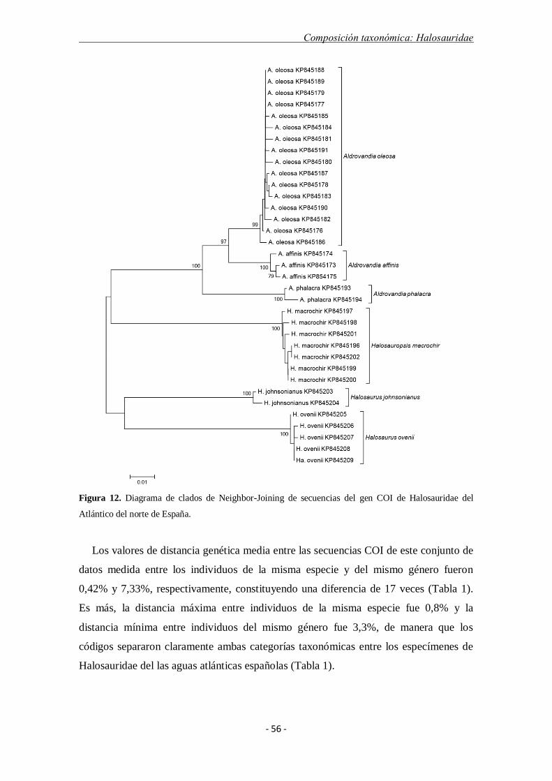
Composición taxonómica: Halosauridae
- 56 -
Figura 12. Diagrama de clados de Neighbor-Joining de secuencias del gen COI de Halosauridae del
Atlántico del norte de España.
Los valores de distancia genética media entre las secuencias COI de este conjunto de
datos medida entre los individuos de la misma especie y del mismo género fueron
0,42% y 7,33%, respectivamente, constituyendo una diferencia de 17 veces (Tabla 1).
Es más, la distancia máxima entre individuos de la misma especie fue 0,8% y la
distancia mínima entre individuos del mismo género fue 3,3%, de manera que los
códigos separaron claramente ambas categorías taxonómicas entre los especímenes de
Halosauridae del las aguas atlánticas españolas (Tabla 1).

Composición taxonómica: Halosauridae
- 57 -
Tab
la 1
. D
ista
nci
as g
enét
icas
(%
p-d
ista
nci
a) e
ntr
e se
cuen
cias
CO
I d
e ej
empla
res
de
Hal
osa
uri
dae
del
Atl
ánti
co d
el n
ort
e de
Esp
aña (
el r
ango d
e
val
ore
s se
mues
tra
entr
e par
énte
sis)
.
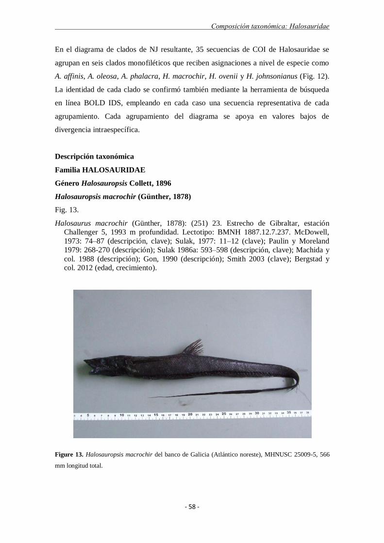
Composición taxonómica: Halosauridae
- 58 -
En el diagrama de clados de NJ resultante, 35 secuencias de COI de Halosauridae se
agrupan en seis clados monofiléticos que reciben asignaciones a nivel de especie como
A. affinis, A. oleosa, A. phalacra, H. macrochir, H. ovenii y H. johnsonianus (Fig. 12).
La identidad de cada clado se confirmó también mediante la herramienta de búsqueda
en línea BOLD IDS, empleando en cada caso una secuencia representativa de cada
agrupamiento. Cada agrupamiento del diagrama se apoya en valores bajos de
divergencia intraespecífica.
Descripción taxonómica
Familia HALOSAURIDAE
Género Halosauropsis Collett, 1896
Halosauropsis macrochir (Günther, 1878)
Fig. 13.
Halosaurus macrochir (Günther, 1878): (251) 23. Estrecho de Gibraltar, estación
Challenger 5, 1993 m profundidad. Lectotipo: BMNH 1887.12.7.237. McDowell,
1973: 74–87 (descripción, clave); Sulak, 1977: 11–12 (clave); Paulin y Moreland
1979: 268-270 (descripción); Sulak 1986a: 593–598 (descripción, clave); Machida y
col. 1988 (descripción); Gon, 1990 (descripción); Smith 2003 (clave); Bergstad y
col. 2012 (edad, crecimiento).
Figure 13. Halosauropsis macrochir del banco de Galicia (Atlántico noreste), MHNUSC 25009-5, 566
mm longitud total.

Composición taxonómica: Halosauridae
- 59 -
Material examinado. MHNUSC 25009-1, 536 mm LT, 7 de agosto de 2011, banco
de Galicia, 42º41.771'N—11º33.647'W, 1477 m; MHNUSC 25009-2, 528 mm LT, 8 de
agosto de 2011, banco de Galicia; 42º43.536'N—11º28.128, 1751 m; MHNUSC 25009-
3, 604 mm LT, 8 de agosto de 2011, banco de Galicia; 42º43.536'N—11º28.128; 1,751
Tab
la 2
. C
om
paa
tiv
a de
los
dat
os
bio
mét
rico
s , m
erís
tico
s y d
e su
s p
roporc
iones
res
pec
to a
l cu
erpo (
%L
GP
) en
los
ejem
pla
res
de H
alo
sau
rop
sis
macr
och
ir.

Composición taxonómica: Halosauridae
- 60 -
m; MHNUSC 25009-4, 585 mm LT, 8 de agosto de 2011, banco de Galicia;
42º43.536'N—11º28.128, 1751 m; MHNUSC 25009-5, 566 mm LT, 29 de julio de
2011, banco de Galicia; 42º56.172'N—11º 55.816’W, 1545 m; MHNUSC 25009-6, 626
mm LT, 29 de julio de 2011, banco de Galicia, 42º56.172'N —11º 55.816’W, 1545 m;
MHNUSC 25009-7, 579 mm LT, 29 de julio de 2011, banco de Galicia, 42º56.172'N—
11º 55.816’W; 1545 m.
Descripción. Cuerpo anguiliforme, moderadamente comprimido y alargado,
atenuándose hacia el pedúnculo caudal; parte superior del rostro sin escamas, opérculo
con escamas; cabeza deprimida anteriormente, distancia interorbital ancha, contenida
4,8–6, 2 veces en la cabeza; origen de la dorsal ligeramente por detrás del origen de las
ventrales; primer radio dorsal segmentado y de igual longitud que el segundo; aleta
pectoral larga y estrecha, alcanzando al menos la base de la dorsal y contenida 1,2–1,3
veces en la cabeza; línea lateral pigmentada, formada por escamas de mayor tamaño que
las del cuerpo; ciegos pilóricos largos, de color crema, dispuestos en una sóla fila. Las
principales medidas morfométricas y caracteres merísticos se presentan en la Tabla 2.
Hábitat y Distribución. Bentopelágico, en el talud inferior y montañas submarinas,
entre 1100 y 3300 m. Cosmopolita: Atlántico este, desde Irlanda hasta Mauritania y
Sudáfrica; Atlántico central, a lo largo de la dorsal atlántica; Atlántico oeste, incluyendo
Canadá hasta 25°N y sur de Brasil; Pacífico oeste, incluyendo Australia, Nueva Zelanda
y Japón; y océano Índico occidental (Sulak, 1986a; Bergstad y col., 2012).
Género Halosaurus Johnson, 1864
Halosaurus ovenii Johnson, 1864
Fig. 14.
Halosaurus ovenii Johnson, 1864: 406, Pl. 26 (fig. 1). Holotipo (único): BMNH
1863.12.12.1. McDowell, 1973: 56–66 (descripción, clave); Sulak, 1977: 11–12
(clave); Sulak, 1986a: 593–598 (descripción, clave); Sulak, 1986b (descripción,
clave); Mceachran y Fechhelm 1998: 210-215 (descripción, clave); Smith, 2003
(clave).

Composición taxonómica: Halosauridae
- 61 -
Figure 14. Halosaurus ovenii del banco de Galicia (Atlántico noreste), MHNUSC 25010-2, 578 mm
longitud total.
Material examinado. MHNUSC 25010-1, 538 mm LT, 4 de agosto de 2011, banco
de Galicia, 42º41.771'N—11º33.647'W, 916 m; MHNUSC 25010-2, 578 mm LT, 29 de
julio de 2009, banco de Galicia, 42º 73.58'N—11º73.580'W, 779 m; MHNUSC 25010-
3, 516 mm LT, 29 de julio de 2009, banco de Galicia, 42º 73.58'N—011º73.580'W, 779
m; MHNUSC 25010-4, 517 mm LT, 29 de julio de 2009, banco de Galicia, 42º
73.58'N—011º73.580'W, 779 m; MHNUSC 25010-5, 523 mm LT, 27 de agosto de
2009, banco de Galicia, 42º 73.58'N—011º73.580'W, 779 m.
Descripción. Cuerpo anguiliforme, moderadamente comprimido y alargado,
atenuándose hacia el pedúnculo caudal; parte superior y lados de la cabeza, hasta el
extremo anterior de la mandíbula inferior, y opérculo, con escamas; rostro relativamente
corto, contenido 2,4-2,6 veces en la cabeza; base de las ventrales anterior a la base de la
dorsal; dientes palatinos dispuestos en la línea media del paladar; interior de la boca
oscura con zonás pálidas características; escamas de la línea lateral (ELL) no
pigmentadas y sólo ligeramente más grandes que las escamas del cuerpo; ciegos
pilóricos pálidos. Las principales medidas morfométricas y caracteres merísticos se
presentan en la Tabla 3.
Hábitat y Distribución. Especie bentopelágica, desde 440 hasta 2800 m de
profundidad, pero más frecuentemente a profundidades menores de 800 m (D'Onghia y
col., 2004). Presente a ambos lados del Atlántico y en el mar Mediterráneo. En el

Composición taxonómica: Halosauridae
- 62 -
Atlántico este se encuentra en el sur de Irlanda, golfo de Vizcaya, España, Portugal,
islas de Madeira, Azores y Canarias y costa occidental de África, desde Marruecos hasta
Sudáfrica (Quéro y col., 1994; Sulak, 1990; Bañón y col., 1997) y en el Atlántico oeste
desde Nueva York hasta Colombia, incluyendo el golfo de México, mar Caribe y las
Antillas (McEachran y Fechhelm, 1998; Saavedra-Díaz y col., 2004); sólo unos pocos
registros en el mar Mediterráneo (Pais y col., 2009).
Ta
bla
3.
Com
paa
tiva
de
los
dat
os
bio
mét
rico
s , m
erís
tico
s y d
e su
s p
rop
orc
ion
es r
espec
to a
l cu
erpo
(%
LG
P)
en l
os
ejem
pla
res
de
Ha
losa
uru
s ove
nii
.
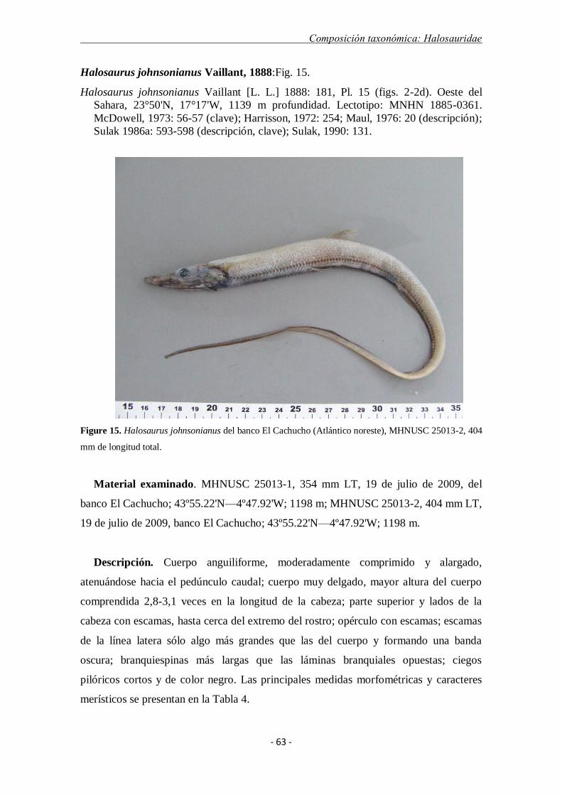
Composición taxonómica: Halosauridae
- 63 -
Halosaurus johnsonianus Vaillant, 1888:Fig. 15.
Halosaurus johnsonianus Vaillant [L. L.] 1888: 181, Pl. 15 (figs. 2-2d). Oeste del
Sahara, 23°50'N, 17°17'W, 1139 m profundidad. Lectotipo: MNHN 1885-0361.
McDowell, 1973: 56-57 (clave); Harrisson, 1972: 254; Maul, 1976: 20 (descripción);
Sulak 1986a: 593-598 (descripción, clave); Sulak, 1990: 131.
Figure 15. Halosaurus johnsonianus del banco El Cachucho (Atlántico noreste), MHNUSC 25013-2, 404
mm de longitud total.
Material examinado. MHNUSC 25013-1, 354 mm LT, 19 de julio de 2009, del
banco El Cachucho; 43º55.22'N—4º47.92'W; 1198 m; MHNUSC 25013-2, 404 mm LT,
19 de julio de 2009, banco El Cachucho; 43º55.22'N—4º47.92'W; 1198 m.
Descripción. Cuerpo anguiliforme, moderadamente comprimido y alargado,
atenuándose hacia el pedúnculo caudal; cuerpo muy delgado, mayor altura del cuerpo
comprendida 2,8-3,1 veces en la longitud de la cabeza; parte superior y lados de la
cabeza con escamas, hasta cerca del extremo del rostro; opérculo con escamas; escamas
de la línea latera sólo algo más grandes que las del cuerpo y formando una banda
oscura; branquiespinas más largas que las láminas branquiales opuestas; ciegos
pilóricos cortos y de color negro. Las principales medidas morfométricas y caracteres
merísticos se presentan en la Tabla 4.

Composición taxonómica: Halosauridae
- 64 -
Hábitat y Distribución. Bentopelágico, entre 680 y 2100 m de profundidad y 4-
11ºC. Atlántico este, desde Porcupine Seabight, Portugal y sur de España hasta
Tab
la 4
. C
om
paa
tiva
de
los
dat
os
bio
mét
rico
s , m
erís
tico
s y
de
sus
pro
po
rcio
nes
res
pec
to a
l cu
erpo (
%L
GP
) en
los
ejem
pla
res
de
Halo
sauru
s jo
hnso
nia
nus.

Composición taxonómica: Halosauridae
- 65 -
Mauritania, incluyendo las islas Azores, Cabo Verde y Canarias (Maul, 1976; Sulak,
1990; Priede y col., 2010).
Genus Aldrovandia Goode & Bean, 1896
Aldrovandia affinis Günther 1877
Fig. 16.
Halosaurus affinis, Günther 1877: 444. Sur de Japón, 34°N, 138°E, estación Challenger
235, 1033 m de profundidad. Sintipos: BMNH 1887.12.7.244-245 (2). McDowell,
1973: 91–101 (descripción, clave); Maul, 1976: 22 (descripción); Filatova, 1985: 27-
29 (descripción), 33-34 (clave); Sulak, 1986a: 593–598 (descripción, clave);
Mceachran y Fechhelm, 1998: 210-215 (descripción, clave); Smith, 2003 (clave).
Figure 16. Aldrovandia affinis del banco de Galicia (Atlántico noreste), MHNUSC 25011-2, 486 mm
longitud total.
Material examinado. MHNUSC 25011-1, 423 mm LT, 7 de agosto de 2011, banco
de Galicia; 42º56.172'N—11º55.816'W; 1545 m; MHNUSC 25011-2, 486 mm LT, 7 de
agosto de 2011, banco de Galicia; 42º41.771'N—11º33.647; 1477 m; MHNUSC 25011-
3, 442 mm LT, 2 de agosto de 2011, banco de Galicia; 42º56.172'N—11º55.816; 1545
m.

Composición taxonómica: Halosauridae
- 66 -
Descripción. Cuerpo anguiliforme, moderadamente comprimido y alargado,
atenuándose hacia el pedúnculo caudal; parte superior de la cabeza y opérculo sin
escamas; región preoral del rostro larga, contenida 2-2,2 veces en la longitud del rostro;
primer radio de la dorsal muy corto, semejando una espina; aleta pectoral corta y ancha,
bien separada del origen de la ventral; origen de la dorsal ligeramente por detrás de las
ventrales; el grupo de dientes palatinos se junta en su línea media; ciegos pilóricos
Ta
bla
5.
Com
paa
tiv
a de
los
dat
os
bio
mét
rico
s , m
erís
tico
s y
de
sus
pro
porc
iones
res
pec
to a
l cu
erpo (
%L
GP
) en
los
ejem
pla
res
de A
ldro
vand
ia a
ffin
is.

Composición taxonómica: Halosauridae
- 67 -
negros y ano blanco. Las principales medidas morfométricas y caracteres merísticos se
presentan en la Tabla 5.
Hábitat y Distribución. Bentopelágico, en la parte media e inferior del talud
continental (700-2200 m), principalmente por encima de la isoterma de los 4° C. En
latitudes tropicales y templadas de todos los océanos. Atlántico este, desde el golfo de
Vizcaya, Madeira hasta el Sahara occidental y Sudáfrica; Atlántico oeste, desde Nueva
Inglaterra hasta Florida, golfo de Mexico, islas del Caribe y América del Sur; Indo-
Pacífico, en Zanzibar, Maldivas, Taiwán y Japón y en el Pacífico cemtro-oriental
(Froese y Sampang, 2004;Yeh y col., 2006).
Aldrovandia phalacra (Vaillant 1888)
Fig. 17.
Halosaurus phalacrus, Vaillant [L. L.] 1888: 185, Pl. 15 (fig. 3), 16 (figs. 1-1c).
Marruecos, 1103-2190 m; Sudán, 1250-1435 m; Azores, 37°35'N, 29°26'W, 1442-
2220 m. Lectotipo: MNHN 1885-0382. McDowell, 1973: 91–92 (clave), 105–114
(descripción); Filatova, 1985: 27-29 (descripción), 33-34 (clave); Sulak 1986a: 593–
598 (descripción, clave); Sulak, 1986b: 196–197 (descripción, clave); Maul, 1976:
20-22 (descripción); Smith, 2003 (clave).
Figure 17. Aldrovandia phalacra del banco de Galicia (Atlántico noreste), MHNUSC 25014-2, 330 mm
longitud total.

Composición taxonómica: Halosauridae
- 68 -
Material examinado. MHNUSC 25014-1, 190 mm LT, 7 de agosto de 2011, banco
de Galicia; 42º41.771'N—011º33.647'W; 1536 m; MHNUSC 25012-2, 330 mm LT, 6
de agosto de 2011, banco de Galicia; 42º41.771'N—11º33.647'W; 1477 m.
Tab
la 6
. C
om
paa
tiva
de
los
dat
os
bio
mét
rico
s , m
erís
tico
s y
de
sus
pro
po
rcio
nes
res
pec
to a
l cu
erpo (
%L
GP
) en
los
ejem
pla
res
de
Ald
rova
ndia
phala
cra
.
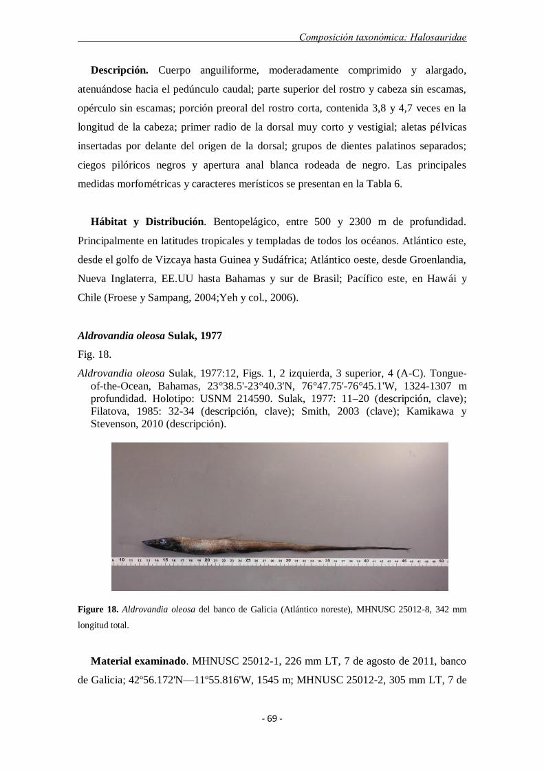
Composición taxonómica: Halosauridae
- 69 -
Descripción. Cuerpo anguiliforme, moderadamente comprimido y alargado,
atenuándose hacia el pedúnculo caudal; parte superior del rostro y cabeza sin escamas,
opérculo sin escamas; porción preoral del rostro corta, contenida 3,8 y 4,7 veces en la
longitud de la cabeza; primer radio de la dorsal muy corto y vestigial; aletas pélvicas
insertadas por delante del origen de la dorsal; grupos de dientes palatinos separados;
ciegos pilóricos negros y apertura anal blanca rodeada de negro. Las principales
medidas morfométricas y caracteres merísticos se presentan en la Tabla 6.
Hábitat y Distribución. Bentopelágico, entre 500 y 2300 m de profundidad.
Principalmente en latitudes tropicales y templadas de todos los océanos. Atlántico este,
desde el golfo de Vizcaya hasta Guinea y Sudáfrica; Atlántico oeste, desde Groenlandia,
Nueva Inglaterra, EE.UU hasta Bahamas y sur de Brasil; Pacífico este, en Hawái y
Chile (Froese y Sampang, 2004;Yeh y col., 2006).
Aldrovandia oleosa Sulak, 1977
Fig. 18.
Aldrovandia oleosa Sulak, 1977:12, Figs. 1, 2 izquierda, 3 superior, 4 (A-C). Tongue-
of-the-Ocean, Bahamas, 23°38.5'-23°40.3'N, 76°47.75'-76°45.1'W, 1324-1307 m
profundidad. Holotipo: USNM 214590. Sulak, 1977: 11–20 (descripción, clave);
Filatova, 1985: 32-34 (descripción, clave); Smith, 2003 (clave); Kamikawa y
Stevenson, 2010 (descripción).
Figure 18. Aldrovandia oleosa del banco de Galicia (Atlántico noreste), MHNUSC 25012-8, 342 mm
longitud total.
Material examinado. MHNUSC 25012-1, 226 mm LT, 7 de agosto de 2011, banco
de Galicia; 42º56.172'N—11º55.816'W, 1545 m; MHNUSC 25012-2, 305 mm LT, 7 de

Composición taxonómica: Halosauridae
- 70 -
agosto de 2011, banco de Galicia, 42º56.172'N—11º55.816'W, 1545 m; MHNUSC
25012-3, 274 mm LT, 7 de agosto de 2011, banco de Galicia, 42º56.172'N—
11º55.816'W, 1545 m; MHNUSC 25012-4, 317 mm LT, 7 de agosto de 2011, banco de
Galicia, 42º56.172'N—11º55.816'W, 1545 m; MHNUSC 25012-5, 255 mm LT, 7 de
agosto de 2011, banco de Galicia, 42º56.172'N—11º55.816'W, 1545 m; MHNUSC
25012-6, 269 mm LT, 7 de agosto de 2011, banco de Galicia, 42º41.771'N—
011º33.647'W, 1477 m; MHNUSC 25012-7, 330 mm LT, 8 de agosto de 2011, banco
de Galicia; 42º43.536'N—11º28.128'W; 1751 m depth; MHNUSC 25012-8, 342 mm
LT, 8 de agosto de 2011, banco de Galicia, 42º43.536'N—11º28.128'W, 1751 m;
MHNUSC 25012-9, 333 mm LT, 8 de agosto de 2011, banco de Galicia, 42º43.536'N—
11º28.128'W, 1751 m; MHNUSC 25012-10, 347 mm LT, 8 de agosto de 2011, banco
de Galicia, 42º43.536'N—11º28.128'W, 1751 m; MHNUSC 25012-11, 205 mm LT, 7
de agosto de 2011, banco de Galicia, 42º56.172'N—11º55.816'W,1545 m; MHNUSC
25012-12, 381 mm LT, 7 de agosto de 2011, banco de Galicia, 42º56.172'N—
11º55.816'W, 1545 m; MHNUSC 25012-13, 352 mm LT, 7 de agosto de 2011, banco
de Galicia, 42º56.172'N—11º55.816'W, 1545 m; MHNUSC 25012-14, 259 mm LT, 7
de agosto de 2011, banco de Galicia, 42º56.172'N—11º55.816'W, 1545 m; MHNUSC
25012-15, 397 mm LT, 7 de agosto de 2011, banco de Galicia, 42º56.172'N—
11º55.816'W, 1545 m; MHNUSC 25012-16, 287 mm LT, 7 de agosto de 2011, banco
de Galicia, 42º56.172'N—11º55.816'W, 1545 m.
Descripción. Cuerpo anguiliforme, moderadamente comprimido y alargado,
atenuándose hacia el pedúnculo caudal; escamas ausentes en la parte superior de la
cabeza y opérculo; longitud pre-oral muy corta, contenida de 3 a 5,3 veces en la
longitud del rostro; los dientes palatinos separados de los pterigoideos por una distacia
comprendida entre 0,7 y 1,7 veces su longitud; primer radio de la dorsal vestigial, muy
corto; apertura anal blanca, rodeada por un anillo de tejido oscuro; ciegos pilóricos
negros. Las principales medidas morfométricas y caracteres merísticos se presentan en
la Tabla 7.
Hábitat y Distribución. Bentónico a bentopelágico, en el talud inferior y la parte
superior abisal, entre 1100 y 3300 m de profundidad y principalmente entre las
isotermas de 2 y 4ºC (Sulak, 1990). En latitudes tropicales y templadas de todos los
océanos. Atlántico oeste, desde Canadá hasta Venezuela y las Guyanas; Atlántico este,
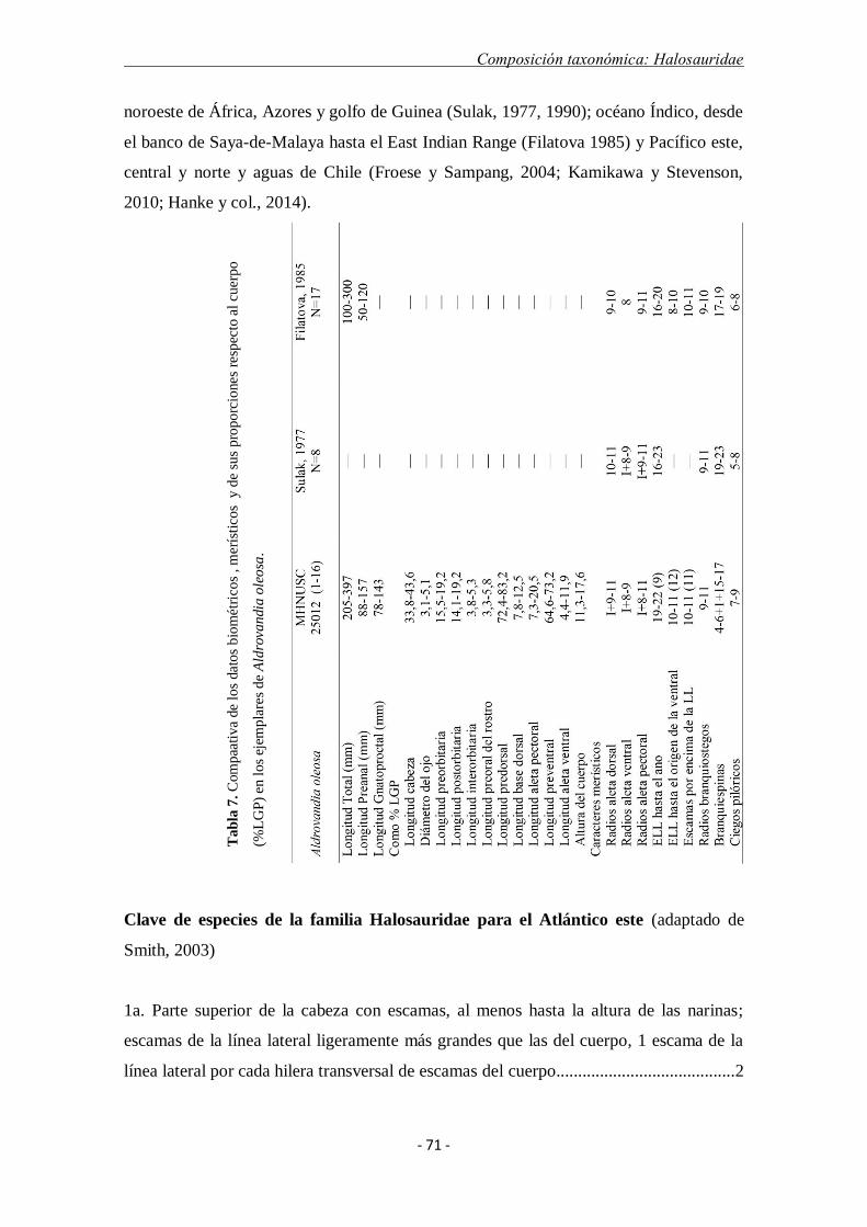
Composición taxonómica: Halosauridae
- 71 -
noroeste de África, Azores y golfo de Guinea (Sulak, 1977, 1990); océano Índico, desde
el banco de Saya-de-Malaya hasta el East Indian Range (Filatova 1985) y Pacífico este,
central y norte y aguas de Chile (Froese y Sampang, 2004; Kamikawa y Stevenson,
2010; Hanke y col., 2014).
Clave de especies de la familia Halosauridae para el Atlántico este (adaptado de
Smith, 2003)
1a. Parte superior de la cabeza con escamas, al menos hasta la altura de las narinas;
escamas de la línea lateral ligeramente más grandes que las del cuerpo, 1 escama de la
línea lateral por cada hilera transversal de escamas del cuerpo.........................................2
Ta
bla
7.
Com
paa
tiv
a de
los
dat
os
bio
mét
rico
s , m
erís
tico
s y
de
sus
pro
porc
iones
res
pec
to a
l cu
erpo
(%L
GP
) en
lo
s ej
emp
lare
s d
e A
ldro
van
dia
ole
osa
.
Composición taxonómica: Halosauridae
- 72 -
1b. Parte superior de la cabeza sin escamas; escamas de la línea lateral notablemente
más grandes que las del cuerpo, 1 escama de la línea lateral por cada 2 a 3 hileras
transversales de escamas del cuerpo .................................................................................5
2a. Parte superior del interior de la boca de color oscuro pero que no se extiende por los
lados hasta la arcada palatopterigoide; parte inferior del interior de la boca oscura,
extendiéndose sólo ligeramente hasta la parte anterior de la lengua, con la parte más
anterior de color claro; de 12 a 20 ciegos pilóricos...............................Halosaurus ovenii
2b. Interior de la boca completamente oscura; de 4 a 12 ciegos
pilóricos.............................................................................................................................3
3a. Longitud de la cabeza aproximadamente 1/4 de la longitud preanal; de 8 a 12 ciegos
pilóricos largos.................................................................................Halosaurus guentheri
3b. Longitud de la cabeza aproximadamente 1/3 de la longitud preanal; de 4 a 9 ciegos
pilóricos cortos..................................................................................................................4
4a. 13-14 branquiespinas en el primer arco branquial, más largas que las láminas
branquiales opuestas...................................................................Halosaurus johnsonianus
4b. 7-12 branquiespinas en el primer arco branquial, más cortas que las láminas
branquiales opuestas........................................................................Halosaurus attenuatus
5a. Primer radio de la dorsal dividido y de igual longitud que el segundo; opérculo con
escamas; ejemplares adultos con la línea lateral oscura; ciegos pilóricos claros y
largos..........................................................................................Halosauropsis macrochir
5b. Primer radio de la dorsal no dividido y mucho más corto que el segundo; opérculo
sin escamas; línea lateral no pigmentada; ciegos pilóricos negros....................................6
6a. Apertura anal azul oscura o negra rodeada de tejido claro..........................................7
6b. Apertura anal blanca rodeada de tejido oscuro............................................................8
7a. Escamas en la línea lateral contiguas; 1 escama de la línea lateral por cada dos
escamas del cuerpo, 22 o 23 anteriores al ano; porción preoral del rostro muy larga,
comprendida menos de 2 veces en la longitud del rostro .................Aldrovandia rostrata
7b. Escamas en la línea lateral no contiguas, separadas por las escamas del cuerpo; 1
escama de la línea lateral por cada 3 escamas del cuerpo, 18 a 20 anteriores al ano;
porción preoral del rostro más corta, comprendida entre 2,25 y 2,5 veces en la longitud
del rostro.............................................................................................Aldrovandia gracilis
8a. Las bandas de dientes palatinos de los dos lados contactan en su parte media; de 13
a 15 branquiespinas en el primer arco branquial; porción preoral del rostro contenida

Composición taxonómica: Halosauridae
- 73 -
aproximadamente 2 veces en la longitud del rostro; origen de la dorsal sobre o muy
ligeramente por detrás de de la base de las aletas ventrales.................Aldrovandia affinis
8b. Las bandas de dientes palatinos de los dos lados separados en su parte media; de 17
a 23 branquiespinas en el primer arco branquial; porción preoral del rostro contenida
aproximadamente 3 veces en la longitud del rostro; origen de la dorsal claramente por
detrás de de la base de las aletas ventrales .......................................................................9
9a. De 24 a 28 escamas en la línea lateral anteriores al ano; dientes palatinos separados
de los pterigoideos por menos de la mitad de su propia longitud; de 11 a 14 radios
pectorales..........................................................................................Aldrovandia phalacra
9b. De 16 a 23 escamas en la línea lateral anteriores al ano; dientes palatinos separados
de los pterigoideos de 1 a 4 veces su propia longitud; de 8 a 11 radios
pectorales..............................................................................................Aldrovandia oleosa
Discusión
La medida de la longitud total en Halosauridae no es precisa, ya que muchos de los
ejemplares tienen la parte final de su frágil cola rota o regenerada. Quizás por esta
razón, hay muchas menos medidas biométricas que datos merísticos en la bibliografía
ictiológica de la familia. Además, las medidas relativas vienen registradas de maneras
diferentes, como porcentajes de la longitud rostro-ano (Kamikawa y Stevenson, 2010),
de la longitud preanal (Filatova, 1985; Gon, 1990; Hsin-Ming y col., 2006), de la
longitud predorsal (Maul, 1976) y de la longitud gnatoproctal (McDowell, 1973; Costa
y Reiner, 1978; Paulin y Moreland, 1979; Machida y col., 1988). La ausencia de un
criterio único en la toma de las biometrías dificulta la comparación entre las especies y
la obtención de un rango de medidas relativas que sirvan como carácter distintivo en la
identificación de especies de Halosauridae. Debido a esta carencia, los datos
comparativos que se muestran en las tablas taxonómicas se basan principalmente en los
caracteres merísticos (Tablas 2-7). La LGP parece ser la biometría más adecuada para
expresar las medida relativas en los halosáuridos, debido a que tanto el rostro como la
cola suelen estar dañados (McDowell, 1973). Por tanto, se recomienda utilizar la LGP
como medida estándar para expresar las medidas relativas en los próximos estudios
taxonómicos de la familia.
La ausencia de escamas en la parte superior de la cabeza distingue H. macrochir de
las especies de Halosaurus, y la presencia de escamas en el opérculo los distingue

Composición taxonómica: Halosauridae
- 74 -
asimismo de las especies de Aldrovandia (Paulin y Moreland, 1979). H. macrochir
difiere también de los otros halosáuridos citados en este trabajo por tener una longitud
interiorbital mayor (6,0-7,9 frente a 2,2-5,3% LGP).
H. ovenii se diferencia de H. johnsonianus por tener mayor número de escamas en la
línea lateral anteriores al ano (61-67 frente a 57), más ciegos pilóricos (12-13 frente a 6-
8) y menos branquiespinas en el primer arco branquial (12-13 frente a 17-18).
Entre las especies de Aldrovandia, A. affinis difiere de las otras dos por tener un
porción preoral más larga, contenida 2-2,2 veces en la longitud del rostro (frente a 3-
5,3) y menos branquiespinas en el primer arco branquial (13-15 frente a 20-25). A.
phalacra difiere de A. oleosa por tener mayor número de escamas en la línea lateral
anteriores al ano (26 frente a 20-22) y más radios pectorales (14-15 frente a 9-12).
De manera general, los datos registrados de distribución latitudinal y en profundidad
están en el rango de estudios anteriores. La excepción la constituye A. oleosa, cuyo
anterior límite norte de distribución estaba en las Azores (Carneiro y col., 2014) y su
presencia en el banco de Galicia constituye un nuevo límite norte de distribución en el
Atlántico este.
Los caracteres merísticos y las medidas biométricas también coinciden con estudios
anteriores, salvo alguna excepción. Según la bibliografía, el ojo de H. johnsonianus es
grande, su diámetro horizontal es aproximadamente un 15% de la longitud de la cabeza
(Vaillant, 1888), 1/6 de la longitud de la cabeza (Sulak, 1986a) o 7,3% de la longitud
preanal (Maul, 1976). Sin embargo, nuestros ejemplares tenían los ojos más pequeños,
6,8 y 10,4% de la longitud de la cabeza o 2,1 y 3% de la longitud preanal,
respectivamente. La presencia de dimorfismo sexual podría ser una posible explicación
a estos resultados, pero el sexo no fue determinado y las biometrías de esta especie,
incluidas el diámetro del ojo, están muy poco documentadas en la bibliografía.
En A. oleosa, los dientes palatinos están bien separados de los pterigoideos, de una a
cuatro veces su propia longitud (Sulak, 1977; Kamikawa y Stevenson, 2010) pero sólo
entre 0,7 y 1,7 veces en los ejemplares de Galicia. Esta separación relativa va a
depender en gran medida de la longitud de la banda de dientes palatinos, que parecen
ser mayores en nuestros ejemplares.
Machida y col. (1988) y Filatova (1985) documentan diferencias geográficas en los
caracteres merísticos de H. macrochir. Nuestros resultados, sin embargo, muestran
también diferencias similares en las otras especies examinadas (Tablas 2-7), que podrían
estar por tanto dentro de las variaciones intraespecíficas normales que se dan en esta

Composición taxonómica: Halosauridae
- 75 -
familia. De hecho, la estructura genética poblacional de H. macrochir no muestra
diferencia genéticas geográficas entre ejemplares del Atlántico norte y del Pacífico
suroeste (David Barros-García comunicación personal).
Los valores de distancia de nucleótidos media entre los individuos de la misma
especie (0,42%) y del mismo género (7,33%) (Tabla 1) están dentro de los valores
habituales de los estudios de código de barras de peces (Costa y col., 2012; Lakra y col.,
2011). La existencia de un claro "barcoding gap" hace de este procedimiento una
herramienta muy útil para la identificación de especies de este grupo. Como muestra, el
código de barras de ADN ha permitido la validación de las identificaciones taxonómicas
de los halosáuridos del Atlántico del norte de España. Otra consecuencia de esta
investigación es la incorporación de treinta y cinco nuevas secuencias de COI en los
repositorios de referencia BOLDSYSTEMS y GenBank, aumentando el número de
muestras de referencia o especímenes ―voucher‖ y el conocimiento de estos peces
relativamente raros. De hecho, este trabajo supone un aumento de un 49,3% en las
secuencias depositadas en BOLDSYTEMS de las seis especies estudiadas (en mayo de
2015). Los códigos de barra de ADN incluyen las cinco especies representadas
históricamente en el Atlántico europeo y la recién descubierta A. oleosa,como se
discutió anteriormente. No se encontraron incongruencias cuando se compararon las
identificaciones morfológicas y moleculares. La identificación morfológica apoya la
identificación molecular y viceversa, reforzando así la identificación resultante. El
incremento del número de códigos de barras disponibles de halosáuridos contribuirá en
el futuro al desarrollo de estudios demográficos y filogenéticos. Esta investigación
constituye un claro ejemplo de taxonomía integrativa (Dayrat, 2005) o de cómo la
técnica del código de barras de ADN se ha integrado con éxito con el análisis
morfológico tradicional en los estudios de sistemática de peces (Baldwin y Weigt,
2012;. Bañón y col., 2013).

Composición taxonómica: Halosauridae
- 76 -
Table S1. Ejemplares de Halosauridae utilizados en el presente estudio y secuencias incluidas en el
análisis de código de barras de ADN.
No. Identificación taxonómica Región BOLD Process ID GenBank Acc. No.
1 Aldrovandia affinis banco de Galicia NOTAC014-15 KP845174
2 Aldrovandia affinis banco de Galicia NOTAC015-15 KP845175
3 Aldrovandia affinis banco de Galicia NOTAC016-15 KP845173
4 Aldrovandia oleosa banco de Galicia NOTAC017-15 KP845185
5 Aldrovandia oleosa banco de Galicia NOTAC018-15 KP845184
6 Aldrovandia oleosa banco de Galicia NOTAC019-15 KP845183
7 Aldrovandia oleosa banco de Galicia NOTAC020-15 KP845182
8 Aldrovandia oleosa banco de Galicia NOTAC021-15 KP845181
9 Aldrovandia oleosa banco de Galicia NOTAC022-15 KP845180
10 Aldrovandia oleosa banco de Galicia NOTAC023-15 KP845179
11 Aldrovandia oleosa banco de Galicia NOTAC024-15 KP845178
12 Aldrovandia oleosa banco de Galicia NOTAC025-15 KP845177
13 Aldrovandia oleosa banco de Galicia NOTAC026-15 KP845176
14 Aldrovandia oleosa banco de Galicia NOTAC027-15 KP845188
15 Aldrovandia oleosa banco de Galicia NOTAC028-15 KP845187
16 Aldrovandia oleosa banco de Galicia NOTAC029-15 KP845191
17 Aldrovandia oleosa banco de Galicia NOTAC030-15 KP845186
18 Aldrovandia oleosa banco de Galicia NOTAC031-15 KP845190
19 Aldrovandia oleosa banco de Galicia NOTAC032-15 KP845189
20 Aldrovandia phalacra banco de Galicia NOTAC068-15 KP845193
21 Aldrovandia phalacra banco de Galicia NOTAC069-15 KP845194
22 Halosauropsis macrochir banco de Galicia NOTAC001-15 KP845201
23 Halosauropsis macrochir banco de Galicia NOTAC002-15 KP845196
24 Halosauropsis macrochir banco de Galicia NOTAC003-15 KP845202
25 Halosauropsis macrochir banco de Galicia NOTAC004-15 KP845200
26 Halosauropsis macrochir banco de Galicia NOTAC005-15 KP845199
27 Halosauropsis macrochir banco de Galicia NOTAC006-15 KP845198
28 Halosauropsis macrochir banco de Galicia NOTAC007-15 KP845197
29 Halosaurus johnsonianus banco El Cachucho
a NOTAC033-15 KP845203
30 Halosaurus johnsonianus banco El Cachucho NOTAC034-15 KP845204
31 Halosaurus ovenii banco de Galicia NOTAC008-15 KP845208
32 Halosaurus ovenii banco de Galicia NOTAC009-15 KP845209
33 Halosaurus ovenii banco de Galicia NOTAC010-15 KP845206
34 Halosaurus ovenii banco de Galicia NOTAC011-15 KP845207
35 Halosaurus ovenii banco de Galicia NOTAC012-15 KP845205

Composición taxonómica: Lepidion
- 77 -
6.4 COMPOSICIÓN DE ESPECIES Y CASOS DE HIPERPIGMENTACIÓN EN EL
GÉNERO LEPIDION (GADIFORMES: MORIDAE) EN EL BANCO DE
GALICIA.
El género Lepidion Swainson, 1838 (Moridae), contiene en la actualidad nueve especies
bentopelágicas que viven en el talud inferior y montes submarinos de los océanos
Atlántico, Índico y Pacífico y del mar Mediterráneo (Nakaya y col., 1980). En el
Atlántico nordeste se han registrados tres especies: Lepidion eques (Günther 1887),
Lepidion guentheri (Giglioli 1880) y Lepidion schmidti Svetovidov 1936 y dos en el
Mediterráneo: L. guentheri y Lepidion lepidion (Risso, 1810) (Cohen, 1986; Quéro y
col., 2003).
Las especies del género Lepidion se caracterizan por tener el cuerpo alargado; rostro
redondeado, con la mandíbula superior prominente; barbillón presente en la mandíbula
inferior; dos aletas dorsales separadas, el segundo radio de la primera aleta dorsal muy
alargado; dientes viliformes en mandíbulas y vómer, ausentes en los palatinos; órgano
luminoso ventral ausente (Templeman, 1970; Nakaya y col., 1980).
Para probar la eficacia de la identificación molecular entre las especies del género
Lepidion, incluyendo ejemplares de L. eques y L. guentheri del BG (ver anexo III), se
han examinado y comparado sus correspondientes códigos de barras de ADN. Se
obtuvieron 32 secuencias de COI propias de cinco especies diferentes de Lepidion, a las
que se sumaron 26 secuencias de otros proyectos presentes en el repositorio BOLD. Se
compararon un total de 58 códigos de barras de ADN pertenecientes a ocho de las nueve
especies conocidas de Lepidion. Las secuencias de COI fueron alineadas y, al ser
comparadas mediante un método bayesiano, formaron siete clados distintos, con las
secuencias de L. lepidion y L. eques agrupadas en el mismo clado. La distancia
interespecífica promedio entre pares de secuencias, según el modelo de 2-parámetros de
Kimura, fue de 4,28%, 16 veces mayor que la obtenida al comparar secuencias de la
misma especie (media = 0,27%).
La distancia entre las secuencias de L. eques y L. lepidion varió entre 0 y 0,62 %
(media = 0,29%), similar a la media intraespecífica de todas las especies del género
(0,27%) y muy por debajo del 2% establecido de manera general como valor mínimo de
distancia para discriminar especies distintas (Hebert y col., 2003, 2004).

Composición taxonómica: Lepidion
- 78 -
Figura 19. Ejemplar de L. eques del banco de Galicia mostrando el radio alargado en la 1ª dorsal
característico del género
Se recopilaron los principales caracteres distintivos del género y se realizó una
revisión morfológica (biometría y merística) de L. eques y L. lepidion (ver anexo III) .
El diámetro del ojo fue significativamente diferente entre L. eques y L. lepidion (P
<0,001). El número de radios de la aleta anal osciló entre 45 y 51 en L. lepidion y de 47
a 54 en L. eques, pero sin diferencias significativas en los valores medios de esta
variable (P = 0,07).
Según Günther (1887), L. eques se puede distinguir de L. lepidion por su ojo,
comparativamente más grande y la cabeza más corta. Sin embargo el estatus de la
especie Atlántica L. eques en relación con su congénere del Mediterráneo L. lepidion ha
sido cuestionado desde principios del siglo XX (Collett, 1905; Roule, 1919).
Finalmente, Templeman (1970) encuentra grandes semejanzas en la merística y las
biometrías de ambas especies, indicando que podrían tener una relación subespecífica,
pero, siguiendo un criterio de precaución, decide no cambiar su estatus.
Los resultados morfológicos muestran una gradación latitudinal descendente norte-
sur en los caracteres merísticos analizados de L. eques, siendo los valores más al sur, del
BG, similares a los de L. lepidion del Mediterráneo. Las diferencias morfológicas con
carácter diagnóstico encontradas pueden ser en realidad los extremos de la variación
latitudinal de la misma especie relacionadas probablemente con la temperatura del agua.
Las información biológica y oceanográfica también sugiere la ausencia de barreras
biogeográficas que delimiten dos especies distintas en Atlántico y Mediterráneo. Los
huevos y las primeras fases de desarrollo de los móridos son pelágicas (Cohen, 1986).
Si bien los huevos de Lepidion están aun sin describir, la fase juvenil pelágica está
descrita en varias especies como L. eques (Saemundsson, 1926; Koefoed, 1927), L.
lepidion (Templeman, 1970) y L. inosimae (Okamoto y col. 2009). El estrecho de
Gibraltar comunica ambos mares y se estima que alrededor del 59% de los peces del
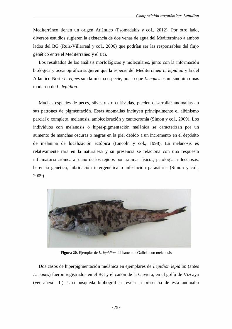
Composición taxonómica: Lepidion
- 79 -
Mediterráneo tienen un origen Atlántico (Psomadakis y col., 2012). Por otro lado,
diversos estudios sugieren la existencia de dos venas de agua del Mediterráneo a ambos
lados del BG (Ruiz-Villarreal y col., 2006) que podrían ser las responsables del flujo
genético entre el Mediterráneo y el BG.
Los resultados de los análisis morfológicos y moleculares, junto con la información
biológica y oceanográfica sugieren que la especie del Mediterráneo L. lepidion y la del
Atlántico Norte L. eques son la misma especie, por lo que L. eques es un sinónimo más
moderno de L. lepidion.
Muchas especies de peces, silvestres o cultivadas, pueden desarrollar anomalías en
sus patrones de pigmentación. Estas anomalías incluyen principalmente el albinismo
parcial o completo, melanosis, ambicoloración y xantocromía (Simon y col., 2009). Los
individuos con melanosis o hiper-pigmentación melánica se caracterizan por un
aumento de manchas oscuras o negras en la piel debido a un incremento en el depósito
de melanina de localización ectópica (Lincoln y col., 1998). La melanosis es
relativamente rara en la naturaleza y su presencia se relaciona con una respuesta
inflamatoria crónica al daño de los tejidos por traumas físicos, patologías infecciosas,
herencia genética, hibridación intergenérica o infestación parasitaria (Simon y col.,
2009).
Figura 20. Ejemplar de L. lepidion del banco de Galicia con melanosis
Dos casos de hiperpigmentación melánica en ejemplares de Lepidion lepidion (antes
L. eques) fueron registrados en el BG y el cañón de la Gaviera, en el golfo de Vizcaya
(ver anexo III). Una búsqueda bibliográfica revela la presencia de esta anomalía
Composición taxonómica: Lepidion
- 80 -
cromática en otros dos ejemplares del mismo género, el primero de ellos en un L.
lepidion del Mediterráneo a finales del siglo XIX (Moreau, 1881).
Macroscópicamente, la hiperpigmentación se caracteriza por la presencia de
numerosas manchas oscuras e irregulares sobre la cabeza, cuerpo y aletas.
Microscópicamente, la melanosis se corresponde con una proliferación hiperplásica de
melanóforos dérmicos. Aunque la causa de la proliferación hiperplásica de células
pigmentadas no se pudo determinar, se propuso la posible acción de agentes etiológicos.
Este trabajo es el primer estudio histopatológico de un ejemplar melánico del género
Lepidion.
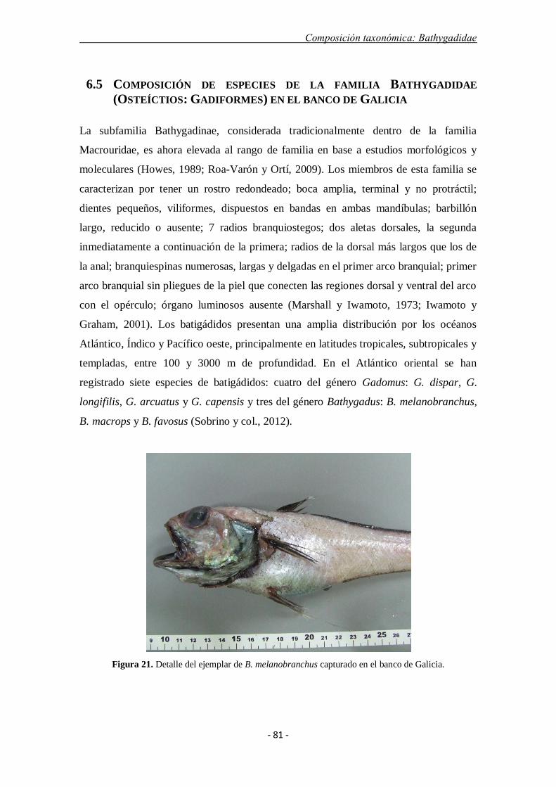
Composición taxonómica: Bathygadidae
- 81 -
6.5 COMPOSICIÓN DE ESPECIES DE LA FAMILIA BATHYGADIDAE
(OSTEÍCTIOS: GADIFORMES) EN EL BANCO DE GALICIA
La subfamilia Bathygadinae, considerada tradicionalmente dentro de la familia
Macrouridae, es ahora elevada al rango de familia en base a estudios morfológicos y
moleculares (Howes, 1989; Roa-Varón y Ortí, 2009). Los miembros de esta familia se
caracterizan por tener un rostro redondeado; boca amplia, terminal y no protráctil;
dientes pequeños, viliformes, dispuestos en bandas en ambas mandíbulas; barbillón
largo, reducido o ausente; 7 radios branquiostegos; dos aletas dorsales, la segunda
inmediatamente a continuación de la primera; radios de la dorsal más largos que los de
la anal; branquiespinas numerosas, largas y delgadas en el primer arco branquial; primer
arco branquial sin pliegues de la piel que conecten las regiones dorsal y ventral del arco
con el opérculo; órgano luminosos ausente (Marshall y Iwamoto, 1973; Iwamoto y
Graham, 2001). Los batigádidos presentan una amplia distribución por los océanos
Atlántico, Índico y Pacífico oeste, principalmente en latitudes tropicales, subtropicales y
templadas, entre 100 y 3000 m de profundidad. En el Atlántico oriental se han
registrado siete especies de batigádidos: cuatro del género Gadomus: G. dispar, G.
longifilis, G. arcuatus y G. capensis y tres del género Bathygadus: B. melanobranchus,
B. macrops y B. favosus (Sobrino y col., 2012).
Figura 21. Detalle del ejemplar de B. melanobranchus capturado en el banco de Galicia.
Composición taxonómica: Bathygadidae
- 82 -
Once ejemplares de cuatro especies de batigádidos (familia Bathygadidae) fueron
capturados entre los años 2009 y 2011 en aguas del norte de España, nueve en el BG y
dos en el cañón de Avilés (ver anexo IV). Las medidas morfométricas al milímetro
inferior y los caracteres merísticos fueron tomados según Marshall e Iwamoto (1973).
Los ejemplares fueron identificados como pertenecientes a los géneros Gadomus Regan,
1903 y Bathygadus Günther, 1878, incluyendo las siguientes especies: Gadomus dispar
(Vaillant, 1888), Gadomus longifilis (Goode y Bean, 1885), Gadomus arcuatus (Goode
y Bean, 1886) y Bathygadus melanobranchus Vaillant, 1888 (Fig. 21). Como resultado
de este estudio, se establece un nuevo límite norte de distribución de G. arcuatus en el
Atlántico noreste.
La identificación molecular de las especies de la familia Bathygadidae se ha
explorado mediante el examen y la comparación de las secuencias de nucleótidos de los
códigos de barras de ADN (ver anexo IV). Las secuencias correspondientes a los
ejemplares de las mismas especies fueron idénticas, dando lugar a un único haplotipo
por especie. La diversidad nucleotídica (distancia p) global media fue de 9,6%. La
diversidad global media intragenérica fue de 5,6% en Bathygadus y de 8% en Gadomus.
La distancia media entre los dos géneros fue de 11,5%. La mayor divergencia
encontrada se dio entre secuencias de COI de B. melanobranchus y G. arcuatus (12,4%)
mientras que los valores menores ocurrieron entre B. antrodes y B. favosus (5,1%).
La taxonomía integrativa se define como la ciencia que tiene por objetivo delimitar la
diversidad de unidades de vida de maneras múltiples y complementarias (Dayrat, 2005).
Para ello, el código de barras de ADN se ha ido implementando en la identificación de
peces junto con los tradicionales análisis morfológicos (Bañón y col., 2014).
Los análisis realizados en la familia Bathygadidae no solo no muestran divergencias
entre los resultados morfológicos y moleculares sino que éstos se refuerzan
mutuamente, incrementando notablemente la fiabilidad de las identificaciones
taxonómicas realizadas.
Composición taxonómica: Bibliografía
- 83 -
6.6 BIBLIOGRAFÍA
Abecasis, D., Cardigos, F., Almada, F. & Gonçalves, J.M.S. 2009.. New records on the
ichthyofauna of the Gorringe seamount (Northeastern Atlantic). Marine Biology
Research, 5: 605–611
Alcázar, J.L., González, P., Fernández, C.L., García, L., Rucabado, J., Lloris, D. &
Castellón, A. 1992. Prospecciones pesqueras en aguas profundas (Sector VIIIc-
ICES). Recursos Pesqueros de Asturias, 6: 1–128.
Baldwin, C.C. & Weigt, L.A. 2012. A new species of soapfish (Teleostei: Serranidae:
Rypticus), with redescription of R. subbifrenatus and comments on the use of
DNA barcoding in systematic studies. Copeia, 1: 23–36.
Bañón, R., Casas, J.M., Piñeiro, C.G. & Covelo, M. 1997. Capturas de peces de
afinidades tropicales en aguas atlánticas de Galicia (NO de la península Ibérica)
Boletín del Instituto Español de Oceanografía, 13: 57–66.
Bañón, R., Arronte, J.C., Barros-García, D., Vázquez-Dorado, S. & de Carlos, A. 2013.
Taxonomic study of Bathygadidae fishes (Gadiformes) from Atlantic Spanish
waters combining morphological and molecular approaches. Zootaxa, 3746:
552–566.
Bañón, R., Barros-García, D., Mucientes, G. & de Carlos, A. 2014. Northernmost
records of Pagrus auriga (Sparidae) and Pomadasys incisus (Haemulidae) in the
eastern Atlantic. Acta Ichthiologica et Piscatoria, 44: 323–327.
Bergstad, O.A., Clark, L., Hansen, H.Ø. & Cousins, N. 2012. Distribution, population
biology, and trophic ecology of the deepwater demersal fish Halosauropsis
macrochir (Pisces: Halosauridae) on the Mid-Atlantic Ridge. PLoS ONE 7,
e31493.
Black, M., Hill, M.N., Laughton, A.S. & Matthews, D.H. 1964. Three non-magnetic
seamounts off the Iberian coast. Quarterly Journal of the Geological Society of
London, 120: 477–513.
Carneiro, M., Martins, R., Landi, M. & Costa, F.O. 2014. Updated checklist of marine
fishes (Chordata: Craniata) from Portugal and the proposed extension of the
Portuguese continental shelf. European Journal of Taxonomy, 73: 1–73.

Composición taxonómica: Bibliografía
- 84 -
Christiansen, B., Vieira, R.P., Christiansen, S., Denda, A., Oliveira, F. & Gonçalves,
J.M.S. 2015. The fish fauna of Ampère Seamount (NE Atlantic) and the adjacent
abyssal plain. Helgoland Marine Research, 69: 13–23.
Clark, M.C. 2009. Deep-sea seamount fisheries: a review of global status and future
prospects. Latin American Journal of Aquatic Research, 37: 501–512.
Cohen, D.M. 1986. Moridae. In: Whitehead, P.J.P., Bauchot, M-L., Hureau, J-C.,
Nielsen, J. & Tortonese, E. (Eds.), Fishes of the Northeastern Atlantic and the
Mediterranean. UNESCO, Paris, pp. 713–723.
Collett, R. 1905. Fiske, indsamlede under “Michael Sars”s Togter I Nordhavet 1900-
1902. Rep on Nor Fishery and Mar Investigations, 2: 1-151.
Compagno, L.J.V. 1988. Sharks of the order Carcharhiniformes. Princeton University
Press, 572 pp.
Costa, M.J. & Reiner, F. 1978. First record of Halosaurus ovenii Johnson, 1863 and
Echiostoma barabatum Lowe, 1843 (Pisces, Halosauridae and
Melanostomatidae) off Portugal. Boletim da Sociedade Portuguesa de Ciências
Naturais, 18: 43–46.
Costa, F.O., Landi, M., Martins, R., Costa, M.H., Costa, M.E., Carneiro, M., Alves,
M.J., Steinke, D. & Carvalho, G.R. 2012. A ranking system for reference
libraries of DNA barcodes: application to marine fish species from Portugal.
PLoS ONE, 7, e35858.
Dayrat, B. 2005. Towards integrative taxonomy. Biological Journal of the Linnean
Society, 85: 407–415.
D'Onghia, G., Lloris, D., Politou, C.-Y., Sion, L. & Dokos, J. 2004. New records of
deep-water teleost fish in the Balearic Sea and Ionian Sea (Mediterranean Sea).
Scientia Marina, 68: 171–183.
Edgar, R.C. 2004. MUSCLE: multiple sequence alignment with high accuracy and high
throughput. Nucleic Acids Research, 32: 1792–1797.
Eschmeyer, W.N. 2015. Catalog of Fishes, genera, species, references. Electronic
version. Available from:
http://research.calacademy.org/research/ichthyology/catalog/fishcatmain.asp
(accessed 1 May 2015)
Federhen, S. 2011. Comment on „„birdstrikes and barcoding: can DNA methods help
make the airways safer?‟‟. Molecular Ecology Resources, 11: 937–938.

Composición taxonómica: Bibliografía
- 85 -
Felsenstein, J. 1985. Confidence limits on phylogenies: an approach using the bootstrap.
Evolution, 39: 783–791.
Filatova, N.A. 1985. Halosaurus (Notacanthiformes) of the Indian Ocean. Journal of.
Ichthyology, 25: 22–35.
Froese, R. & Sampang, A. 2004. Preliminary annotated checklist of seamount fishes. In:
Morato, T. & Pauly, D. (Eds.), Seamounts: Biodiversity and Fisheries. Fisheries
Centre Research Report 12, pp. 1–73.
Froese, R. & Pauly, D. 2016. FishBase. World Wide Web electronic publication.
www.fishbase.org, version (01/2016).
George, M.R. & Zidowitz, H. 2006. Checkliste der europäischen Knorpelfischarten mit
wissenschaftlichen und deutschen Namen. Zeitschrift für Fischkunde, 8: 71-81
Gon, O. 1990. Halosauridae. In: Gon, O. & Heemstra, P.C. (Eds.), Fishes of the
Southern Ocean. J.L.B. Smith Institute of Ichthyology, South Africa,
Grahamstown, pp. 98–99.
Günther, A. 1887. Report on the deep-sea fishes collected by H. M. S. Challenger
during the years 1873-76. Report of the Scientific Results of the Voyage of
H.M.S. Challenge, 22: 1–268.
Hanke, G.F., Gillespie, G., Fong, K., Boutillier, J., Peden, A.E. & Bedard, J.M. 2014.
New records of spiny eels (Albuliformes), true eels (Anguilliformes), and
bobtail eels (Saccopharyngiformes) in British Columbia, Canada. Northwestern
Naturalist, 95: 63–76.
Harrisson, C.M.H. 1972. Halosauridae of the North Eastern Atlantic (Pisces, Teleostei,
Notacanthiformes). Bulletin du Muséum national d'histoire naturelle (Zoologie),
40: 553–560.
Hebert, P.D.N., Cywinska, A., Ball, S.L. & De Waard, J.R. 2003. Biological
identifications through DNA barcodes. Proceedings of the Royal Society of
London Series B, 270: 313–321.
Hebert, P.D.N., Penton, E.H., Burns, J.M., Janzen, D.H. & Hallwachs, W. 2004. Ten
species in one: DNA barcoding reveals cryptic species in neotropical skipper
butterfly Astraptes fulgerator. Proceedings of the National Academy of Sciences
of the United States of America, 101: 14812–14817.

Composición taxonómica: Bibliografía
- 86 -
Hsin-Ming, Y., Mao-Ying, L. & Kwang-Tsao, S. 2006. Three new records of halosaurid
fishes (Pisces: Halosauridae) from the deep-waters adjacent to Taiwan. Journal
of The Fisheries Society of Taiwan, 33: 345–355.
Howes, G.J. 1989. Phylogenetic relationships of macrouroid and gadoid fishes based on
cranial myology and anthology. In: Cohen, D.M. (Ed.), Papers on the
systematics of gadiform fishes. Natural History Museum of Los Angeles County,
Los Angeles, pp. 112–128.
Hubbs, C.L. 1959. Initial discoveries of fish faunas on seamounts and offshore banks in
the eastern Pacific. Pacific Science, 13: 311-316.
Iglésias, S.P. & Nakaya, K. 2004. Apristurus atlanticus (Koefoed, 1927), a junior
synonym of A. laurussonii (Saemundsson, 1922) (Chondrichthyes:
Carcharhiniformes: Scyliorhinidae). Cybium, 28: 217–223.
Iglésias, S.P., Lecointre, G. & Sellos, D.Y. 2005. Extensive paraphylies within sharks of
the order Carcharhiniformes inferred from nuclear and mitochondrial genes.
Molecular Phylogenetics and Evolution, 34: 569–583.
Ivanova, N.V., Zemlak, T.S., Hanner, R.H. & Hebert, P.D.N. 2007. Universal primer
cocktails for fish DNA barcoding. Molecular Ecology Notes, 7: 544–548.
Iwamoto, T. & Graham, K. 2001. Grenadiers (Families Bathygadidae and Macrouridae,
Gadiformes, Pisces) of New South Wales, Australia. Proceedings of the California
Academy of Sciences, 52: 407–509.
Iglesias, S.P., Lecointre, G. & Sellos, D.Y. 2005. Extensive paraphylies within sharks of
the order Carcharhiniformes inferred from nuclear and mitochondrial genes.
Molecular Phylogenetics and Evolution, 34: 569–583.
Kamikawa, D.J. & Stevenson, D.E. 2010. Aldrovandia oleosa (Notacanthiformes:
Halosauridae): first record from the eastern North Pacific. California Fish and
Game, 96: 216–220.
Klimpel, S., Palm, H.W., Busch, M.W. & Kellermanns, E. 2008. Fish parasites in the
bathyal zone: the halosaur Halosauropsis macrochir (Günther, 1878) from the
Mid Atlantic Ridge. Deep Sea Research Part II: Topical Studies in
Oceanography, 55: 229–235.
Koefoed, E. 1927. Fishes of the sea-bottom. Report on the Scientific Results of the
Michael Sars Atlantic Deep-Sea Expedition 1910, 4: 1–148

Composición taxonómica: Bibliografía
- 87 -
Koslow, J.A, Boehlert, G.W, Gordon, J.D.M., Haedrich, R.L., Lorance, P. & Parin, N.
2000. Continental slope and deep-sea fisheries: implications for a fragile
ecosystem. ICES Journal of Marine Science, 57: 548–557.
Lakra, W.S, Verma, M.S., Goswami, M., Lal, K.K., Mohindra, V., Punia, P.,
Gopalakrishnan, A., Singh, K.V., Ward, R.D. & Hebert, P. 2011. DNA
barcoding Indian marine fishes. Molecular Ecology Resources, 11: 60–71.
Lincoln, R., Boxshall, G. & Clark, P. 1998. A dictionary of ecology, evolution and
systematics. Cambridge University Press, Cambridge, UK. 361 pp.
Machida, Y., Okamura, O. & Ohta, S. 1988. Notes on Halosauropsis macrochir
(Halosauridae: Notacanthiformes) from Japan. Japanese Journal of Ichthyology,
35: 78–82.
Maisey, J.G. 1984. Higher elasmobranch phylogeny and biostratigraphy. Zoological
journal of the Linnean Society, 82: 33–54.
Marshall, N.B. & Iwamoto, T. 1973. Family Macrouridae. In: Cohen, D.M. et al. (Eds.),
Fishes of the Western North Atlantic. Memoirs of the Sears Foundation of
Marine Research, New Haven, pp. 496–665.
Maul G.E. 1976. The fishes taken in bottom trawls by R.V. „Meteor‟ during the 1967
seamounts cruises in the northeast Atlantic. Meteor Forschungsergebnisse, 22:
1–69.
McClain, C.R. 2007. Seamounts: identity crisis or split personality? Journal of
Biogeography, 34: 2001-2008.
McDowell, B.C. 1973. Family Halosauridae. In: Cohen, D.M. et al. (Eds.), Fishes of the
Western North Atlantic. Memoirs of the Sears Foundation of Marine Research,
New Haven, pp. 32–123.
McEachran, J.D. & Fechhelm, J.D. 1998. Fishes of the Gulf of Mexico. Vol. 1:
Myxiniformes to Gasterosteiformes. University of Texas Press, Austin, 1120 pp.
Menezes, G.M., Rosa, A., Melo, O. & Porteiro, F. 2012. Annotated list of demersal
fishes occurring at Sedlo Seamount, Azores north-east central Atlantic Ocean.
Journal of Fish Biology, doi:10.1111/j.1095-8649.2012.03355.x
Mohn, C. 2010. Spotlight 5: Great Meteor Seamount. Oceanography, 23: 106–107.
Morato, T., Cheung, W.W.L. & Pitcher, T.J. 2006. Vulnerability of seamount fish to
fishing: fuzzy analysis of life history attributes. Journal of Fish Biology, 68:
209–221.

Composición taxonómica: Bibliografía
- 88 -
Morato, T. & Clark, M.R. 2007. Seamount Fishes: Ecology and Life Histories. In:
Pitcher, T.J., Morato, T., Hart, P.J.B., Clark, M.R., Haggan, N. & Santos, R.S.
(Eds.), Seamounts: Ecology, Fisheries and Conservation. Fish and Aquatic
Resources Series, Blackwell, Oxford, UK. pp. 170–188.
Morato, T., Varkey, D.A., Dâmaso, C, Machete, M., Santos, M., Prieto, R., Santos, R.S.
& Pitcher, T.J. 2008. Evidence of a seamount effect on aggregating visitors.
Marine Ecology Progress Series, 357: 23–32.
Morato, T., Hoyle, S.D., Allain, V. & Nicol, S.J. 2010. Seamounts are hotspots of
pelagic biodiversity in the open ocean, Proceedings of the National Academy of
Sciences of the United States of America, 107: 9707–9711.
Moreau, E. 1881. Histoire naturelle des poissons de la France. G. Masson, Paris, 698 pp.
Nakaya, K., Amaoka, K. & Abe, K. 1980. A review of the genus Lepidion (Gadiformes,
Moridae) from the Northwestern Pacific. Japanese Journal of Ichthyology, 27:
41–47.
Nakaya, K. & Sato, K. 1999. Species grouping within thegenus Apristurus
(Elasmobranchii, Scyliorhinidae). In: Séret B. & J.-Y. Sire (Eds.), Proceedings
5th Indo-Pacific Fish Conference. Société Françaised‟Ichtyologie & Institut de
Recherche pour le Développement, Paris, pp. 307–320.
Nei, M. & Kumar, S. 2000. Molecular evolution and phylogenetics. Oxford University
Press, New York, 333 pp.
Nelson, J.S. 2006. Fishes of the world. John Wiley and Sons, Hoboken, New Jersey, 601
pp.
Niklitschek, E.J., Cornejo-Donoso, J., Oyarzún, C., Hernández, E. & Toledo, P. 2010.
Developing seamount fishery produces localized reductions in abundance and
changes in species composition of bycatch. Marine Ecology, 31: 168–182.
Okamoto, M., Watanabe, Y. & Asahida, T. 2009. Descriptive morphology of pelagic
juvenile of Lepidion inosimae (Gadiformes: Moridae) collected from off
northeastern Japan. Ichthyological Researchs, 56: 76–81.
Pais, A., Merella, P., Follesa, M.C. & Motomura, H. 2009. North-easternmost record of
Halosaurus ovenii (Actinopterygii: Notacanthiformes: Halosauridae) in the
Mediterranean Sea, with notes on its biology. Acta Ichthyologica et Piscatoria,
39: 33–37.
Paulin, C.D. & Moreland, J.M. 1979. Halosauridae of the south west Pacific (Pisces:
Teleostei: Notacanthiformes). New Zealand Journal of Zoology, 6: 267–271.

Composición taxonómica: Bibliografía
- 89 -
Pitcher, T.J. 2010. Box 8: Eight major target species in world seamount fisheries.
Oceanography, 23: 130–131.
Priede, I.G., Godbold, J.A., King, N.J., Collins, M.A., Bailey, D.M. & Gordon, J.D.M.
2010. Deep-sea demersal fish species richness in the Porcupine Seabight, NE
Atlantic Ocean: global and regional patterns. Marine Ecology, 31: 247–260.
Psomadakis, P.N., Giustino, S. & Vacchi, M. 2012. Mediterranean fish biodiversity: an
updated inventory with focus on the Ligurian and Tyrrhenian seas. Zootaxa,
3263: 1–46
Quéro, J.C., Porche, P. & Vayne, J.J. 2003. Guide des poissons de l‟Atlantique européen.
Delachaux et Niestlé, Paris, 465 pp.
Quéro, J.C., du Buit, M.H., Fonteneau, J., Laborde, J., Morandeau, L.G. & Vayne, J.J.
1994. Observations Ichtyologiques effectuées en 1993. Annales de la Société des
Sciences Naturelles de la Charente-Maritime, 8: 359–369.
Roa-Varón, A. & Ortí, G. 2009. Phylogenetic relationships among families of
Gadiformes (Teleostei, Paracanthopterygii) ased on nuclear and mitochondrial
data. Molecular Phylogenetics and Evolution, 52: 688–704.
Rogers, A.D. 1994. The biology of seamounts. Advances in Marine Biology, 30: 305–
350.
Rolán, E. & Pedrosa, G.P.G. 1981. Molluscs collected at the Galizia Bank (Spain). La
Conchiglia, 13: 6–7.
Roule, L. 1919. Poissons provenant des campagnes du yacht 'Princesse Alice' (1891-
1913) et du yacht 'Hirondelle II' (1914). Résultats des Campagnes scientifiques
du Prince Albert Ier de Monaco, 52: 1–191.
Ruiz-Villarreal, M., Gonzalez-Pola, C., Diaz del Rio, G., Lavin, A., Otero, P.,
Piedracoba, S. & Cabanas, J.M. 2006. Oceanographic conditions in North and
North West Iberia and their influence on the Prestige oil spill. Marine Pollution
Bulletin, 53: 220–238.
Saavedra-Díaz, L.M., Roa-Varón, A., Acero-P., A. & Mejía, L.S. 2004. Nuevos registros
ícticos en el talud superior del Caribe colombiano (Ordenes Albuliformes,
Anguilliformes, Osmeriformes, Stomiiformes, Ateleopodiformes, Aulopiformes
y Pleuronecetiformes). Boletín de investigaciones marinas y costeras, 33: 181–
207.
Saemundsson, B. 1926. Bláriddari (H. eques Gthr). In: Íslensk Dýr I. Fiskarnir.
Reykjavík. 273-274.

Composición taxonómica: Bibliografía
- 90 -
Saitou, N. & Nei, M. 1987. The neighbor-joining method: A new method for
reconstructing phylogenetic trees. Molecular Biology and Evolution, 4: 406–425.
Samad, I.S., Bottan, L., Macpherson, E., Richer de Forges, B. & Boisselier, M.C. 2006.
Seamount endemism questioned by the geographic distribution and population
genetic structure of marine invertebrates. Marine Biology, 149: 1463–1475.
Sato, K., Nakaya, K. & Stewart, A.L. 1999. A new species of the deep-water catshark
genus Apristurus from New Zealand waters (Chondrichthyes: Scyliorhinidae).
Journal of the Royal Society of New Zealand 29: 325– 335.
Sato, K. 2000. Phylogenetic systematics of the deep-water catsharks genus Apristurus
(Chondrichthyes, Carcharhiniformes, Scyliorhinidae). PhD thesis, Hokkaido
University, Faculty of Fisheries, 132 pp.
Secretariat of the Convention on Biological Diversity. 2008. Synthesis and review of the
best available scientific studies on priority areas for biodiversity conservation in
marine areas beyond the limits of national jurisdiction. Technical Series, 37.
Secretariat of the Convention on Biological Diversity, Montreal, 63 pp.
Simon, T., Joyeux, J.C. & Macieira, R.M. 2009. First record of partial melanism in the
coney Cephalopholis fulva (Perciformes: Epinephelidae). Brazilian Journal of
Oceanography, 57: 145–147.
Smith, D.G. 1999. Halosauridae. In: Carpenter, K.E. & Niem, V.H. (Eds.), FAO species
identification guide for fishery purposes. The living marine resources of the
Western Central Pacific. Batoid fishes, chimaeras and bony fishes part 1
(Elopidae to Linophrynidae). FAO, Rome, pp. 1625–1626.
Smith, D.G. 2003. Halosauridae. In: Carpenter, K.E. (Ed.). FAO species identification
guide for fishery purposes. The living marine resources of the Western Central
Atlantic. Bony fishes part 1 (Acipenseridae to Grammatidae). FAO, Rome, pp:
685–687.
Sobrino, I., González, J., Hernández-González, C.L. & Balguerias, E. 2012. Distribution
and relative abundance of main species of grenadiers (Macrouridae, Gadiformes)
from the African Atlantic coast. Journal of Ichthyology, 52: 690–699.
Srivathsan, A. & Meier, R. 2012. On the inappropriate use of Kimura-2-parameter (K2P)
divergences in the DNA-barcoding literature. Cladistics, 28: 190–194.
Strona, G., Galli, P. & Fattorini, S. 2013. Fish parasites resolve the paradox of missing
coextinctions. Nature Communications, 4, 1718.

Composición taxonómica: Bibliografía
- 91 -
Sulak, K.J. 1977. Aldrovandia oleosa, a new species of the Halosauridae, with
observations on several other species of the family. Copeia, 1: 11–20.
Sulak, K.J. 1986a. Halosauridae. In: Whitehead, P.J.P. Bauchot, M.-L. Hureau, J.-C.
Nielsen J. & Tortonese, E. (Eds.), Fishes of the north-eastern Atlantic and the
Mediterranean. UNESCO, Paris, pp: 593–598.
Sulak, K.J. 1986b. Halosauridae. In: Smith, M.M. & Heemstra, P.C. (Eds.), Smith's sea
fishes. Macmillan South Africa, Johannesburg, pp: 196–197.
Sulak, K.J. 1990. Halosauridae. In: Quéro, J.C. Hureau, J.C., Karrer, C. Post, A. &
Saldanha, L. (Eds.) Check-list of the fishes of the eastern tropical Atlantic
(CLOFETA), UNESCO, JNICT & SEI, Lisboa, Paris, pp: 126-132.
Tamura, K., Stecher, G., Peterson, D., Filipski, A. & Kumar, S. 2013. MEGA6:
Molecular Evolutionary Genetics Analysis Version 6.0. Molecular Biology and
Evolution, 30: 2725–2729.
Templeman, W. 1970. A review of the morid fish genus Lepidion of the North Atlantic
with first records of Lepidion eques from the western North Atlantic. Journal of
the Fisheries Research Board of Canada, 27: 457–498.
Vaillant, L.L. 1888. Expéditions scientifiques du "Travailleur" et du "Talisman" pendant
les années 1880, 1881, 1882, 1883. Poissons. G. Masson, Paris, 406 pp.
Ward, R.D., Zemlak, T.S., Ines, B.H., Last, P.R. & Hebert, P.D.N. 2005. DNA barcoding
Australia‟s fish species. Philosophical Transactions of the Royal Society B, 360:
1847–1857.
Ward, R. D., Hanner, R. & Hebert, P.D.N. 2009. The campaign to DNA barcode all
fishes, FISH-BOL. Journal of Fish Biology, 74: 329–3565.
Wiley, E.O. & Johnson, G.D. 2010. A teleost classification based on monophyletic
groups. In: Nelson, J.S. Schultze, H.-P. & Wilson, M.V.H. (Eds.), Origin and
phylogenetic interrelationships of teleosts. Verlag Dr. Friedrich Pfeil, Germany,
München, pp: 123–182.
Williams, A., Last, P.R., Gomon, M.F. & Paxton, J.R. 1996. Species composition and
checklist of the demersal ichthyofauna of the continental slope off Western
Australia (20-35°5). Records of the Western Australian Museum, 18: 135–155.
Winchell, C.J., Martin, A.P. & Mallatt, J. 2004. Phylogeny of elasmobranchs based on
LSU and SSU ribosomal RNA genes. Molecular Phylogenetics and Evolution,
31: 214–224.

Composición taxonómica: Bibliografía
- 92 -
Yeh, H.M., Lee, M.Y. & Shao, K.T. 2006. Three new records of halosaurid fishes
(Pisces: Halosauridae) from the deep waters adjacent to Taiwan. Journal of the
Fisheries Society of Taiwan, 33: 345–355.
Zemlak, T.S., Ward, R.D., Connell, A.D., Holmes, B.H. & Hebert, P.D.N. 2009. DNA
barcoding reveals overlooked marine fishes. Molecular Ecology Resources, 9:
237–242.
Zhang, Z-Q. 2011. Animal biodiversity: An introduction to higher-level classification
and taxonomic richness. Zootaxa, 3148: 7–12.

Conclusiones
- 93 -
7 CONCLUSIONES
1. La aplicación de la taxonomía integrativa, utilizando análisis complementarios
morfológicos y moleculares (código de barras de ADN), resulta en identificaciones
más fiables y veraces.
2. Por el número de especies identificadas, el banco de Galicia es una zona de alta
biodiversidad ictiológica, superior al de las montañas submarinas más próximas del
entorno de las Azores.
3. Las especies de aguas profundas ("deep water fishes"), que viven habitualmente
a profundidades mayores de 400 m, constituyen la mayoría de las especies que
componen el banco de Galicia.
4. El ochenta y uno por ciento de las especies de peces registradas en el banco de
Galicia fueron registradas anteriormente en otras montañas submarinas y por tanto
pueden ser categorizados como peces de montañas submarinas.
5. El setenta y uno por ciento de las especies de peces del banco de Galicia han
sido citadas con anterioridad en el talud o plataforma de Galicia, pero la práctica
totalidad de las especies ya habían sido registradas en aguas del Atlántico europeo,
indicando la ausencia de especies endémicas en el banco de Galicia.
6. La mayoría de las especies fueron capturadas dentro del rango de presencia de
corales de agua fría, entre 620 y 1125 m de profundidad, indicando una posible
asociación que es preciso confirmar.
7. Se ha constatado que la actividad pesquera en el banco de Galicia ha sido escasa
y ha ido disminuyen con el tiempo, ejercida principalmente con artes de pesca poco
destructivos como volantas y palangres, lo que ha mantenido el ecosistema del
banco de Galicia en un buen estado de conservación.
8. Especies como Aldrovandia oleosa, Physiculus dalwigki, Pseudophychthys
splendens o Gaidropsarus granti, que tenían anteriormente su límite norte de
distribución en el Atlántico este en las Azores, son citadas ahora en el banco de
Galicia, pareciendo indicar una distribución a saltos ("stepping stones") utilizando
las islas y montañas submarinas.
9. Los análisis morfológicos y moleculares junto con la información biológica y
oceanográfica sugieren que la especie endémica del Mediterráneo L. lepidion y la

Conclusiones
- 94 -
del Atlántico norte L. eques son en realidad la misma especie, por lo que L. eques es
un sinónimo más moderno de L. lepidion.
10. La alta biodiversidad encontrada y porcentaje de especies vulnerables presentes
en el banco de Galicia recomiendan su protección y ratifican su declaración como
Lugar de Importancia Comunitaria (LIC) realizada recientemente por la Unión
Europea (Ejecución UE 2015/2373 de la Comisión de 26 de noviembre de 2015).

Anexo I
- 95 -
ANEXO I
Bañón, R., J.C. Arronte, C. Rodríguez-Cabello, C.-G. Piñeiro, A. Punzón & A.
Serrano. 2016. Commented checklist of marine fishes from the Galicia Bank seamount
(NW Spain). Zootaxa. 4067 (3): 293–333
Anexo I
- 96 -
Abstract A commented checklist containing 139 species of marine fishes recorded at
the Galician Bank seamount is presented. The list is based on nine prospecting and
research surveys carried out from 1980 to 2011 with different fishing gears. The
ichthyofauna list is diversified in 2 superclasses, 3 classes, 20 orders, 62 families and
113 genera. The largest family is Macrouridae, with 9 species, followed by Moridae,
Stomiidae and Sternoptychidae with 7 species each. The trachichthyd Hoplostethus
mediterraneus and the morid Lepidion lepidion were the most abundant species.
Biogeographically, the Atlantic group, with 113 species (81.3%) is the best represented,
followed by the Lusitanian one with 17 species (12.2%). Data on species abundance, as
number of individuals caught, size and depth are reported. Habitat, distribution and
vulnerability status are commented. Moreover, biometric data and meristic counts are
also reported for several species. The results obtained showing a high fish biodiversity
and a sensible number of threatened species, strongly support the future declaration of
the Galicia Bank as a Marine Protected Area.
Introduction
Seamounts are typically defined as submarine mountains that rise at least 1000 m from
the abyssal floor of the ocean but do not reach the surface. However, there is not a
general accepted definition, having being extensively modified in the literature
according to the author‘s disciplines (Staudigel et al. 2010). In fact, the Galicia Bank
aside from a seamount, has been defined in many different ways, such as a structural
high (Ercilla et al. 2006; Alonso et al. 2008), a submarine bank (Ruiz-Villareal et al.
2006) or a microplate (Sibuet et al. 2007). In the North East Atlantic, seamounts are
defined according to the Oslo-Paris Convention (OSPAR) as undersea mountains of
volcanic origin, with a crest that rises more than 1000 m above the surrounding seafloor
(Howell et al. 2010).
The number of seamounts is difficult to estimate, but, according to the Census of
Marine Life, there are potentially up to 100,000 seamounts over 1 km high and many
more of smaller elevation. Seamounts biodiversity is still poorly understood on a global
scale due to the lack of prospecting and exploratory surveys. Thus, very few seamounts
have been studied so far; only about 350 seamounts have been sampled and less than
200 have been surveyed in any detail, many of them located in waters within national
jurisdiction (Secretariat of the Convention on Biological Diversity 2008).

Anexo I
- 97 -
Available research results suggest that seamounts are often highly productive
ecosystems known for their ability to support high biodiversity and special biological
communities, including cold-water coral reefs, abundant fishery resources, marine
mammals and seabirds (Johnston & Santillo 2004).
The Galicia Bank seamount was described for the first time by Black et al.
(1964). The first biological study was on fossil benthonic foraminifera (Fisher 1969).
The geophysical and geological studies were carried out focussing on its geodynamic
origins, evolution and magnetic field (Black et al. 1964; Sibuet et al. 1978; Vanney et
al. 1979).
Unfortunately, on 19 November 2002, the Galicia Bank gained international
notoriety with the sinking of the ‗‗Prestige‘‘ oil tanker in the south-western part of the
Bank. As a result of this environmental catastrophe, the area was the object of intensive
and multidisciplinary studies, resulting in many scientific papers mainly related to
marine pollution and geology (Albaigés et al. 2006; Ercilla & Vilas 2008).
The available biological information on the Galicia Bank showed a low benthic
biomass dominated by filter feeders (Duineveld et al. 2004). The Bank is characterized
by the presence of live and dead cold-water corals Lophelia pertusa and Madrepora
oculata, both of high ecological importance (Bouchet & Metivier 1988; Somoza et al.
2014). The rest of the macrofauna is diverse and includes mainly corals (Scleractinia,
Octocorallaires), mollusks (bivalves, gastropods, aplacophora), echinoderms (including
some stalked crinoids and ophiuroids), polychaetes (Nereidae and Polynoidae) sponges
(Demospongiae and Hexactinellida) and decapod crustaceans (decapods, euphausiids,
peracarids, ostracods) (Rolán & Pedrosa 1981; Flach et al. 2002; Duineveld et al. 2004;
Cristobo et al. 2010; Cartes et al. 2014)
Compared with the surrounding ocean waters, seamounts support a great
diversity of fish species, which may form dense aggregations for spawning or feeding
and are generally targeted by large-scale fisheries (Clark et al. 2006). The ichthyofauna
of the Galicia Bank is not well known. The first records have been reported in the
decade of 1980 in grey literature and since the late 1990's in scientific journals. The first
compilation reported the presence of 86 fish species in this area: 70 teleosts, 11 sharks,
3 rays and 2 chimaeras (Piñeiro et al. 2001). However, these authors only provided the
scientific name of 19 species. Bañón et al. (2010) included in a checklist of marine

Anexo I
- 98 -
fishes from Galician waters the ones captured until 2009 in the Galicia Bank, but
without distinguishing between fishes captured in the continental shelf and in the Bank.
There is a need for large-scale management and conservation of deep-sea
biodiversity and ecosystem function, including the establishment of networks of marine
protected areas (MPAs) on the High Seas, including the seamounts (Clark et al. 2011).
The Galicia Bank is one of the eleven areas proposed by the Spanish Ministry for
Agriculture, Food and Environment (Ministerio de Agricultura, Alimentación y Medio
Ambiente) to be designated, first as a special area of conservation (SAC) for species and
habitats, under the Habitat Directive (Council Directive 92/43/EEC), and finally as part
of the Natura 2000 network of MPAs in the North East Atlantic Ocean. In order to
obtain the information required to fulfil the SAC proposal and begin conservation and
management actions, the project LIFE+ "Inventory and designation of marine Natura
2000 areas in the Spanish sea (INDEMARES)‖ (EC contract INDEMARES-LIFE,
07/NAT/E/0007) was conducted (www.indemares.es). In addition, the Galicia Bank is
one of the areas under evaluation in the habitat monitoring in the European Union‘s
Marine Strategy Framework Directive (2008/56/CE). In both Habitats and Marine
Strategy directives, the presence of vulnerable and threatened species listed on
international conventions such as the Convention for the Protection of the Marine
Environment of the North-East Atlantic (OSPAR) or the International Union for
Conservation of Nature (IUCN), is one of the key factors in conservation actions.
The aim of this investigation is to present an updated and commented check list of the
marine fishes currently known in the Galicia Bank and to briefly discuss the results
obtained.
Material and Methods
Study area. The Galicia Bank is an isolated non-volcanic large seamount, located in the
Northwestern of the Iberian Peninsula (North-east Atlantic), between 42° 15′N and
43°N and from 11° 30′W to 12° 15′W, at water depths from 625 to 1,800 m and
approximately 125 nautical miles offshore the coast (Fig. 1). The Bank has an extension
of about 2117 km2
and shows a trapezoidal shape of 75 km wide in the NNE-SSO
direction and 58 km length in the ONO-ESE direction mostly bounded by a steep scarp
(Cristobo et al. 2014; Somoza et al. 2014). A peak in the Eastern zone of the bank
comes within 625 m of the surface. To the North, Northwest it slopes very steeply from
Anexo I
- 99 -
approximately 1,000 m down to the abyssal plain at 5,000 m, and is separated from the
Iberian continental margin by a 3000 m depth channel.
The Bank is part of the Galicia Bank region, an area of complex morphology,
which is divided, from east to west, in five physiographic provinces: the Galicia Interior
Basin, the Transitional Zone, the Galicia Bank, the Half-Graben province and the Deep
Galicia Margin (Vázquez et al. 2008). The Galicia Bank is formed by series of narrow
(10–20 km) and elongated (60–100 km) blocks tilted to the continent along normal
faults oriented roughly N–S, interrupted and/or slightly displaced by NW–SE and ESE–
WNW transverse faults (Díaz et al. 2007).
The Galicia Bank is under the influence of several thermohaline driven water
masses flowing northwards. These mostly comprise the North Atlantic Central Water, at
depths around 540 m, the Mediterranean Outflow Water, at around 1,490 m, the
Labrador Sea influenced Deep Intermediate Water at around 2,155 m, the Lower North
Atlantic Deep Water at around 3,450 m and the Lower Deep Water below this depth
(Rey et al. 2008).
Sampling, species identification and morphological analysis. Ichthyological
samplings were carried out during three distinct periods between 1980 and 2011 (Table
1). The samplings included both exploratory surveys, conducted by commercial vessels,
and multidisciplinary scientific research surveys, conducted by oceanographic vessels.
Both type of surveys aimed different objectives. The main purposes of the exploratory
surveys were to evaluate the possibility of a long-term sustainable exploitation of the
fisheries resources and also to obtain scientific information (Durán & Román 2000),
whereas the main objective of the INDEMARES scientific surveys was to obtain
information about habitats, species and the environmental conditions required for the
Natura 2000/ SAC proposals.
The present checklist includes the compilation of all fish species recorded in
each survey. However, the taxonomical list obtained during the exploratory surveys
carried out during the decade of 1980 was partial and restricted to the main commercial
species. Therefore, this information was only used to point out the presence of some
epipelagic species reported in these surveys or as complementary information of some
species poorly recorded in the other surveys.

Anexo I
- 100 -
Fish species were collected using many types of fishing gears, including
commercial ones such as bottom trawl, pelagic and bottom longlines, ―piedra-bola‖
longline and scientific sampling gears, mainly beam trawl (10 mm codend mesh size)
and GOC73 otter trawl (20 mm codend mesh size).
TABLE 1. Summary of datasets used for this study.
Year No. Surveys Total days Survey type Gear Acronym
1980 2 37 exploratory multi-gear —
1981 2 23 exploratory multi-gear —
1997 2 13 exploratory longline —
1998 1 5 exploratory longline —
1998 3 13 exploratory bottom trawl —
1999 9 35 exploratory bottom trawl —
2009 1 3 scientific multi-gear Ecomarg0709
2010 1 16 scientific multi-gear BanGal0810
2011 1 13 scientific multi-gear BanGal0811
Only specimens identified to species level have been included in the list. Fish
species were identified according to published keys and guides, mainly Whitehead et al.
(1986) and Quéro et al. (2003), but also following other specific guides and numerous
scientific papers. The checklist is presented in the taxonomic sequence: superclass,
class, order, family, genus and species. Quéro et al. (2003), Eschmeyer (2014) and
Froese & Pauly (2014) were followed for the classification system order, the scientific
nomenclature and the common names respectively.
For the majority of species listed, the total number of captured specimens, their
size or size range, the mean length±SD (only in samples with N≥30), depth or depth
range and the habitat and distribution data are reported. Size was generally reported as
total length (TL) to the nearest cm or mm, with the exception of macrurids (family
Macrouridae), where the preanal length (PAL) was measured. Habitat and distribution
information has been compiled from Ebert & Stehman (2013) for elasmobranches and
from Froese & Pauly (2014) and Whitehead et al. (1986) for teleosts. In addition,
specific literature on several species was used when necessary.

Anexo I
- 101 -
Biometric data and meristic counts were also reported for several species. The
total length, standard length and fork length data are expressed in millimeters and the
rest of the measures as percentage of the standard length.
FIGURE 1. Map of the study area
The following abbreviations were used for morphometric and meristic
characters: total length (TL), standard length (SL), Fork length (FL), Head length (HL),
pre-orbital length (PO), Eye diameter (ED), Post orbital Length (POL), Inter-orbital
width (IOW), barbel length (BL), pre-dorsal length, first, second (PD, PD1, PD2), pre-
anal length (PA), dorsal fin base length, first, second (LD, LD1, LD2), anal fin base
length (LA), pre-pectoral distance (PP), pre-ventral distance (PV), pectoral fin length
(LP),ventral fin length (LV), maximum body height (H), number of rays in dorsal, first,
second (D, 1D, 2D), pectoral (P), ventral (V), anal (A) and caudal (C) fins., total
number of gillrakers on the first gill arch (Gr); number of scales on the lateral line (LL).
For the nomenclature of photophores; ventral-anal (VAV); pectoral-pelvic (PV); lateral
series (OA); ventral series posterior to anal fin origin (AC); isthmus-pectoral (IP); (IC);
subpectoral (PVO); suprapectoral (PLO); thoracic (PO); supraventral (VLO); superanal
(SAO); ventral (VO); anal (AO).

Anexo I
- 102 -
Biogeography and Vulnerability. The attribution of biogeographic affinity categories
was adopted following Ellis et al. (2007): Boreal, Lusitanian (including Mediterranean
species), Atlantic (including deep-water or mesopelagic species widely distributed) and
African.
The vulnerability and conservation status of each fish species were compiled
from two global Red List inventories, IUCN (IUCN 2014; Nieto et al. 2015) and
FishBase (Froese & Pauly 2014) and one regional, OSPAR (OSPAR, 2014). According
to IUCN criteria, species are consider threatened if they are categorized as critically
endangered (CR), endangered (EN) or vulnerable (VU), and non-threatened if
categorized as near threatened (NT), least concern (LC) or data deficient (DD).
According to FishBase criteria (Cheung et al. 2005) species are considered to be
threatened if they are categorized as very high vulnerability (VHV), high to very high
vulnerability (HHV) and high vulnerability (HV) and non-threatened if categorized as
moderate to high vulnerability (MHV), moderate vulnerability (MV), low to moderate
vulnerability (LMV) and low vulnerability (LV). Species listed in the OSPAR list of
threatened and/or declining species were considered as vulnerable (VU).
Results
SUPERCLASS GNATHOSTOMATA
CLASS CHONDRICHTHYES
ORDER HEXANCHIFORMES
Family Hexanchidae
Hexanchus griseus (Bonnaterre, 1788) — Bluntnose sixgill shark
14 specimens were caught at depths between 682 and 1,035 m. Length data were
available for eight females from 130 to 355 cm and one male of 73 cm TL.
Habitat and Distribution: deep-water demersal species inhabiting the outer
continental shelves, upper continental slopes, insular shelves and slopes, and
submarine canyons down to at least 2,500 m depth. Circumglobal in tropical and

Anexo I
- 103 -
temperate seas, including the Mediterranean, Baltic and North Seas and the
Hawaiian Islands. Vulnerability: NT (IUCN), VHV (FishBase).
ORDER SQUALIFORMES
Family Centrophoridae
Centrophorus granulosus (Bloch & Schneider, 1801) — Gulper shark
218 specimens were caught at depths between 823 and 1,119 m. Length data
were recorded for all specimens: two males of 115 cm TL and 216 females
between 107 and 166 cm TL (145.4±12.4). The main biological data of the
specimens of C. granulosus captured in Galician waters, including the Galicia
Bank, were previously reported by Bañón et al. (2008). Habitat and Distribution:
deep-water shark of the outer continental shelves and upper slopes at depths
from 50 to 1,440 m. Widely distributed in all ocean basins except the Eastern
Pacific. Vulnerability: CR (IUCN), VU ( OSPAR), VHV (FishBase).
Centrophorus squamosus (Bonnaterre, 1788) — Leafscale gulper shark
1,329 specimens were caught at depths between 749 and 1119 m. Length data
were available for 1,226 specimens, with males between 88 and 129 cm
(110.9±4.1, N=1,015) and females between 96 and 144 cm (122.2±10.6, N=211)
The main biological data relating to C. squamosus caught in Galician waters,
including the Galicia Bank, were previously reported (Bañón et al. 2006a).
Habitat and Distribution: deepwater gulper shark of the continental slopes from
229 to over 4,000 m depth, but rare above 1,000 m depth. Eastern Atlantic,
Western North Atlantic (one record from Venezuela), Western Indian and
Western Pacific Oceans. Vulnerability: EN (IUCN), VU (OSPAR), VHV
(FishBase).
Deania calcea (Lowe, 1839) — Birdbeak dogfish
Prior to 2009 this species was classified erroneously together with D.
profundorum and since them only 4 males, from 90 to 108 cm TL, were caught
at depths between 851 and 916 m. Habitat and Distribution: outer continental
and insular shelves and upper, middle, and lower slopes from 60 to 1,490 m

Anexo I
- 104 -
depth, but usually at depths between 400 and 900 m. Wide and patchy
distribution in the Eastern Atlantic (Iceland to Southern Africa) and Pacific
Oceans (Chile, Peru, Japan, southern Australia and New Zealand). Vulnerability:
EN (IUCN), HHV (FishBase).
Deania profundorum (Smith & Radcliffe, 1912) — Arrowhead dogfish
Until 2009 this species was misidentified as D. calcea. It was correctly
identified from 2009 based on morphological and molecular approaches
(Sanjuán et al. 2012). 83 specimens were caught at depths between 749 and
1,079 m. Length data were available for 70 specimens ranging from 25 to 88 cm
TL (61.8±17.6), with males between 27 and 76 cm TL (61.9±13.7, N=32) and
females between 25 and 88 cm TL (61.8±20.4, N=38). Habitat and Distribution:
bathydemersal with patchy distribution in Eastern Atlantic, Western Indian and
Western Pacific Oceans from 275 to 1,785 m depth. Vulnerability: LC (IUCN),
HHV (FishBase).
Deania hystricosa (Garman, 1906) — Rough longnose dogfish
4 specimens were caught between 766 and 909 m depth. Only one specimen was
measured, a female of 100 cm TL. Habitat and Distribution: benthic and
probably epibenthic of the upper and middle continental and insular slopes, at
depths between 471 and 1,300 m. Patchily distributed in Eastern Atlantic and
Western North Pacific. Vulnerability: DD (IUCN), HHV (FishBase).
Family Etmopteridae
Etmopterus spinax (Linnaeus, 1758) — Velvet belly lantern shark
2,951 specimens were caught at depths between 643 and 1,115 m. Length data
were available for 1,156 specimens ranging from 13 to 49 cm TL (33.9±7.5),
with males between 13 and 44 cm TL (31.6±6.3, N=446) and females between
13 and 49 cm TL (35.8±7.6, N=680). Habitat and Distribution: bathydemersal,
found on the outer continental shelves and upper slopes at depths of 70–2,000 m,
mostly between 200 and 500 m. Eastern Atlantic, from Iceland and Norway to
Gabon, including the Azores and Cape Verde islands and Western
Mediterranean Sea. Vulnerability: LC (IUCN), MHV (FishBase).
Etmopterus pusillus (Lowe, 1839) — Smooth lanternshark

Anexo I
- 105 -
33 specimens were caught at depths between 643 and 936 m. Length data were
available for 21 specimens ranging from 33 to 47 cm TL, with males between 33
and 45 cm (N=15) and females between 33 and 47 cm (N=6). Habitat and
Distribution: benthopelagic, on the continental slopes, on or near bottom at a
depth of 274 to 1000 m or deeper (possibly up to 1998 m). Eastern Atlantic,
Western Atlantic, Indian, Central and Western Pacific Oceans. Vulnerability: LC
(IUCN), MV (FishBase).
Etmopterus princeps Collet, 1904 — Great lanternshark
25 specimens were caught at depths between 1,460 and 1,809 m. Length data
were recorded for all specimens ranging from 18 to 64 cm TL, with males
between 19 and 64 cm (N=11) and females between 18 and 60 cm (N=14).
Habitat and Distribution: bathydemersal on the continental slopes and also lower
rise from 350 to 4,500 m depth. Eastern North Atlantic, from Greenland and
Iceland to Mauritania and possibly Sierra Leone and Western North Atlantic
(Canada and USA). Vulnerability: DD (IUCN), MHV (FishBase).
Family Somniosidae
Centroscymnus coelolepis Barbosa du Bocage & de Brito Capello, 1864 —
Portuguese dogfish.
318 specimens were caught at depths between 749 and 1,685 m. Length data
were available for 306 specimens ranging from 78 to 120 cm TL (107.3±7.5),
with males between 83 and 100 cm (91.8±3.3, N=34) and females between 78
and 120 cm (109.2±5.3, N=272). The main biological data of the specimens of
C. coelolepis caught in Galician waters, including the Galicia Bank, was
previously reported by Bañón et al. (2006a). Habitat and Distribution:
bathydemersal, inhabits continental and insular slopes and abyssal plains, on or
near the bottom at depths of 128-3,675 m, but mostly below 400 m depth.
Widely distributed in the Atlantic, including Western Mediterranean Sea and
Indian and Pacific Oceans. Vulnerability: EN (IUCN), HV (FishBase), VU
(OSPAR).
Centroselachus crepidater (Barbosa du Bocage & de Brito Capello, 1864) —
Longnose velvet dogfish.

Anexo I
- 106 -
14 specimens were caught at depths between 823 and 1,024 m. Length data were
available for one male of 58 cm TL and 11 females between 74 and 88 cm TL.
Habitat and Distribution: bathydemersal, occurs along upper continental and
insular slopes on or near the bottom at depths of 200 to 1,500 m. Eastern
Atlantic, from Iceland to South Africa and scattered distributed throughout the
Indo–Pacific and Eastern South Pacific from off Chile. Vulnerability: LC
(IUCN), VHV (FishBase).
Scymnodon ringens Barbosa du Bocage & de Brito Capello, 1864 — Knifetooth
dogfish
366 specimens were caught at depths between 712 and 1,470 m. Length data
were available for 185 specimens ranging from 25 to 110 cm TL (69.5±23.2),
with males between 26 and 84 cm (53.3±14.3, N=46) and females between 25
and 110 cm (78±22.1, N=125). Habitat and Distribution: usually mesopelagic,
although captured most often near the bottom at depths from 200 to 1,600 m.
Eastern Atlantic: from Scotland to Mauritania, and Senegal. One specimen
recorded in the South Pacific Ocean. Vulnerability: DD (IUCN), HV (FishBase).
FIGURE 2. Oxynotus paradoxus.
Somniosus rostratus (Risso, 1827) — Little sleeper shark
17 specimens were caught at depths between 822 and 1,119 m. Length data were
recorded for all specimens ranging from 76 to 126 cm TL, with males between
Anexo I
- 107 -
76 and 106 cm (N=7) and females between 89 and 126 cm (N=10). Habitat and
Distribution: outter continental shelves and upper slopes, occurring on or near
the bottom at depths between 180 and 2,200 m. Eastern Atlantic: France,
Portugal, and Madeira Islands, and the Western Mediterranean Sea. Western
Central Atlantic: possibly off Cuba. Vulnerability: DD (IUCN), VHV
(FishBase).
Family Oxynotidae
Oxynotus paradoxus Frade, 1929 — Sailfin roughshark (Fig. 2)
2 specimens were caught at depths between 866 and 877 m. Only one specimen
of 32 cm TL was measured. Habitat and Distribution: continental slope at depths
from 265 to 720 m. Endemic to the Eastern Atlantic, from Scotland and northern
North Sea to Senegal and possibly southwards to the Gulf of Guinea region.
Apparently absent from the Mediterranean Sea. Vulnerability: DD (IUCN), HV
(FishBase).
Family Dalatiidae
Dalatias licha (Bonnaterre, 1788) — Kitefin shark
101 specimens were caught at depths between 731 and 1,115 m. Length data
were available for 37 specimens ranging from 38 to 151 cm TL (117.1±31.8),
with males between 38 and 122 cm (N=10) and females between 42 and 151 cm
(N=26). Habitat and Distribution: deepwater, warm–temperate and tropical
shark of the outer continental and insular shelves and slopes from 37 to at least
1800 m depth, but commonest below 200 m. North-east Atlantic from the north
of the British Isles to the north-western coast of Africa, including Azores and
Madeira Islands and the Mediterranean Sea. Western North Atlantic, central and
Western Pacific, and Indian Oceans. Vulnerability: EN (IUCN), VHV
(FishBase).
ORDER LAMNIFORMES
Family Pentanchidae
Galeus melastomus Rafinesque, 1810 —Blackmouth catshark

Anexo I
- 108 -
One female of 70 cm TL was caught at depths between 669 and 676 m. Habitat
and Distribution: deepwater bottom shark found on the outer continental shelves
and upper slopes, mainly between 200 and 500 m but occasionally up to 55 m
and down to 2000 m. Eastern North Atlantic, from Norway to Senegal and
throughout the Mediterranean Sea. Vulnerability: LC (IUCN), HV (FishBase).
FIGURE 3. Galeus murinus.
Galeus murinus (Collett, 1904) — Mouse catshark (Fig. 3)
18 specimens between 29 and 44 cm TL were caught at a depth range from
1,450 to 1,683 m, with males between 29-41 cm TL (N=5) and females between
31-44 cm (N=13). Habitat and Distribution: Iceland to the Faroe Islands, and
recently it has been found off Scotland, the Hebrides Islands, Ireland, France,
Spain, Morocco, and Western Sahara. Vulnerability: LC (IUCN), MHV
(FishBase).
Apristurus aphyodes Nakaya & Stehmann, 1998 — No common name
18 specimens, 6 males ranging from 24 to 39 cm and 12 females from 22 to 37
cm TL, were caught at a depth range of 1,460–1,809 m. Habitat and
Distribution: bathydemersal deepwater species known from continental slopes,
on or near bottom at depths of 380 to 1,250 m. North Atlantic, from Iceland to
the northern Bay of Biscay. The Galicia Bank records constitute the southern

Anexo I
- 109 -
limit in the distribution of this species (Rodríguez-Cabello et al. 2014).
Vulnerability: DD (IUCN), HHV (FishBase).
Apristurus profundorum (Smith & Radcliffe, 1912) — Arrowhead dogfish
One female of 14 cm TL was caught at 1,459 m depth. Habitat and Distribution:
deepwater shark found on the continental slopes at 1,100 to 1,830 m. Reported
in the western North Atlantic, the mid-Atlantic Ridge and eastern North Atlantic
(Mauritania). This record extends northwards the known distribution of this
species in the Northeast Atlantic (Rodríguez-Cabello et al. 2014). Vulnerability:
DD (IUCN), MHV (FishBase).
Apristurus melanoasper Iglesias, Nakaya and Stehmann, 2004 — Black roughscale
catshark
One female of 25 cm TL was caught at 1,683 m depth. Habitat and Distribution:
widely distributed but very patchy in the North Atlantic, Southeastern Atlantic
(Namibia), Central Indian Ocean and south of Madagascar and in the Western
South Pacific (Australia, New Zealand and New Caledonia). This record extends
the known distribution of this species in the Northeast Atlantic (Rodríguez-
Cabello et al. 2014). Vulnerability: DD (IUCN), MHV (FishBase).
Family Pseudotriakidae
Pseudotriakis microdon de Brito Capello, 1868 — False catshark
32 specimens were caught at depths between 823 and 1,119 m. Length data were
recorded for all specimens ranging from 186 to 256 cm TL (224.1±21.2), with
males between 186 and 220 cm (N=16) and females between 207 and 256 cm
(N=16). Habitat and Distribution: continental and insular slopes at depths from
100 to 1,890 m; occasionally wandering onto continental shelves, even in
shallow water. Sporadically recorded in all Oceans, with the exception of the
South Atlantic and Eastern Pacific. Vulnerability: LC (IUCN), HHV (FishBase).
Family Carcharhinidae
Prionace glauca (Linnaeus, 1758) — Blue shark
5 females ranging between 75-113 cm TL were caught at depth unknown,
during the hauling of bottom longline. In addition, 13 specimens were reported

Anexo I
- 110 -
during the exploratory surveys carried out on the 1980's. Habitat and
Distribution: oceanic epipelagic and fringe-littoral shark, occurring from the
surface to at least 350 m depth; deeper in warm temperate and subtropical
waters. Circumglobal in temperate and tropical waters. Vulnerability: NT
(IUCN), HHV (FishBase).
Isurus oxyrinchus Rafinesque, 1810 — Shortfin mako
Reported only during the exploratory surveys on the 1980's with length range
from 125 to 245 cm TL. Habitat and Distribution: epipelagic, oceanic shark
generally occurs in tropical and warm temperate seas off the continental shelf at
depths of 120 to 240 m or even deeper. North Atlantic Ocean and scattered
records in the Pacific and Western Indian Oceans. Vulnerability: VU (IUCN),
VHV (FishBase).
ORDER RAJIFORMES
Family Rajidae
Dipturus batis (Linnaeus, 1758) — Blue skate
9 specimens were caught at depths between 729 and 896 m. Length data were
available for five specimens ranging from 22 to 146 cm TL. Currently, this
species is under taxonomic revision. According to Iglésias et al. (2010) D. batis
is in fact a composite species and it was provisionally split into the smaller D.
sp. cf. flossada and the much larger D. sp. cf. intermedia. Vulnerability: CR
(IUCN), VHV (FishBase), VU (OSPAR).
Rajella bigelowi (Stehmann, 1978) — Bigelow's ray (Fig. 4)
Two specimens, one male of 53 cm and one female of 42 cm TL, were caught at
depths between 1,450 and 1,683 m. Habitat and Distribution: demersal on
several types of bottom substrate from 650 to up to 4,165 m depth. Eastern
North Atlantic, from Greenland and Iceland to Mauritania. Vulnerability: LC
(IUCN), MV (FishBase).
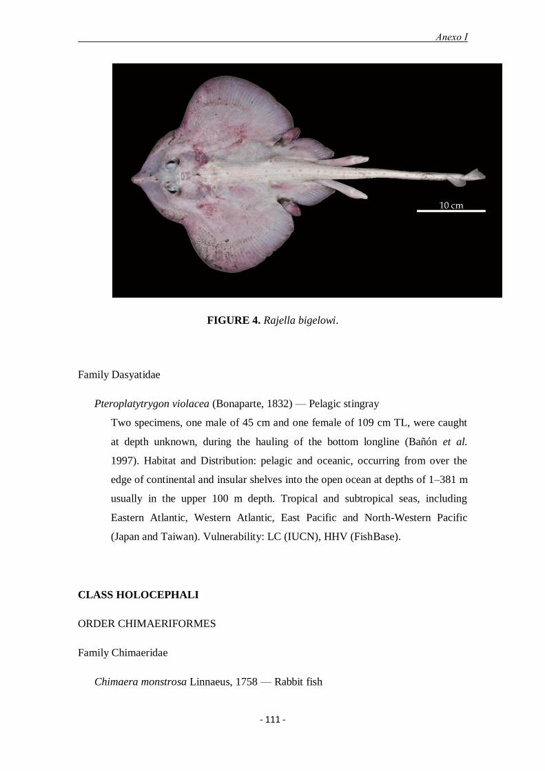
Anexo I
- 111 -
FIGURE 4. Rajella bigelowi.
Family Dasyatidae
Pteroplatytrygon violacea (Bonaparte, 1832) — Pelagic stingray
Two specimens, one male of 45 cm and one female of 109 cm TL, were caught
at depth unknown, during the hauling of the bottom longline (Bañón et al.
1997). Habitat and Distribution: pelagic and oceanic, occurring from over the
edge of continental and insular shelves into the open ocean at depths of 1–381 m
usually in the upper 100 m depth. Tropical and subtropical seas, including
Eastern Atlantic, Western Atlantic, East Pacific and North-Western Pacific
(Japan and Taiwan). Vulnerability: LC (IUCN), HHV (FishBase).
CLASS HOLOCEPHALI
ORDER CHIMAERIFORMES
Family Chimaeridae
Chimaera monstrosa Linnaeus, 1758 — Rabbit fish

Anexo I
- 112 -
3 specimens were caught at depths between 877 and 1,323 m. Dubious
identification specially after the capture of the cryptic species C. opalescens also
in the Bank. Habitat and Distribution: bathydemersal to benthopelagic at depth
range 40-1,000 m, generally between 300 and 500 m depth. Eastern Atlantic:
northern Norway and Iceland, Skagerrak and Kattegat south to Morocco
including western Mediterranean Sea (some isolated records from eastern part),
Azores and Madeira Islands. Records from South Africa are questionable.
Vulnerability: NT (IUCN), HHV (FishBase).
Chimaera opalescens Luchetti, Iglésias & Sellos, 2011 — Opal chimaera
4 specimens, 3 males of 10, 57 and 63 cm and one female of 64 cm TL, were
caught at depths from 903 to 1,450 m. This species was recently described
(Luchetti et al. 2011) and could probably be confused with C. monstrosa in
previous surveys. Habitat and Distribution: Northeast Atlantic, along the slope
to the west of the British Isles and France, from 900-1,400 m depth.
Vulnerability: DD (IUCN), HV (FishBase).
Hydrolagus affinis (de Brito Capello, 1868) — Smalleyed rabbitfish
Three specimens, 2 females of 12 and 22 cm TL and one male of 24 cm, were
caught at depths between 1,683 and 1,808 m. Habitat and Distribution: Found on
continental slopes and down to deep-sea plains, reported up to 3,000 m. Occurs
in North-Eastern Atlantic from the Rockall Trough along Ireland, northern Bay
of Biscay and off Portugal down to 22º off NW Africa, Cape Verde and Azores.
Vulnerability: LC (IUCN), HHV (FishBase).
CLASS ACTINOPTERYGII
ORDER NOTACANTHIFORMES
Family Halosauridae
Halosaurus ovenii Johnson, 1864 — No common name
12 specimens were caught at depths between 746 and 1,536 m. Length data were
available for eight specimens ranging from 20 to 57 cm TL. Habitat and
Distribution: both sides of the Atlantic Ocean, from Madeira, the Azores and

Anexo I
- 113 -
Canaries to Walvis Bay and the Gulf of Mexico, the Caribbean, the Antilles and
the Mediterranean Sea. Vulnerability: DD (IUCN), MHV (FishBase).
FIGURE 5. Halosauropsis macrochir.
Halosauropsis macrochir (Günther, 1878) — Abyssal halosaur (Fig. 5)
7 specimens from 52 to 62 cm TL were caught at depths between 1,536 and
1,809 m. Habitat and Distribution: benthopelagic, 1,100-3,300 m. Antitropical
distribution in Atlantic, Indian, and Pacific Oceans. Vulnerability: DD (IUCN),
MHV (FishBase).
Aldrovandia affinis (Günther, 1877) — Gilbert's halosaurid fish
3 specimens from 42 to 48 cm TL were caught at depths between 1,477 and
1,545 m. Habitat and Distribution: benthopelagic, 730–2,200 m. Worldwide,
known from all major oceans. Vulnerability: DD (IUCN), MHV (FishBase).
Aldrovandia phalacra (Vaillant 1888)— Hawaiian halosaurid fish
2 specimens of 19 and 33 cm TL were caught at a depth of 1,536 and 1,477 m
respectively. Habitat and Distribution: Benthopelagic between 500-2,300 m
depth. Circumglobal, mainly at tropical and temperate latitudes. Vulnerability:
DD (IUCN), MV (FishBase).
Aldrovandia oleosa Sulak, 1977 — No common name

Anexo I
- 114 -
16 specimens from 20 to 39 cm TL were caught at depths between 1,477 and
1,751 m. Benthopelagic to benthic on the lower slope, continental rise and upper
abyss, between 1,100 and 3,300 m depth and primarily between 2 and 4ºC
isotherm. Circumglobal at tropical and temperate latitudes. in Atlantic, Indian,
and Pacific Oceans. Vulnerability: DD (IUCN), MV (FishBase).
Family Notacanthidae
Notacanthus bonaparte Risso, 1840 — Shortfin spiny eel
656 specimens were caught at depths between 731 and 1685 m. Length data
were available for 375 specimens ranging from 15 to 46 cm TL (31.3±6.5).
Habitat and Distribution: bathypelagic between 487-2,000 m depth. Eastern
Atlantic Ocean, Iceland, Faeroes, and from Ireland to Cape Blanc, Mauritania,
and in the Western Mediterranean Sea. Vulnerability: DD (IUCN), LV
(FishBase).
Polyacanthonotus rissoanus (De Filippi & Verany, 1857) — Smallmouth spiny eel
7 specimens between 21 and 43 cm TL were caught at depths between 1,536 snd
1,809 m. Habitat and Distribution: epibenthic anti-tropical on the continental
slope, between 540-2,875 m with most records between 1,500-2,000 m depth.
Eastern Atlantic, from Iceland to South Africa, including the Mediterranean Sea
and Western Atlantic, from Davis Strait to Cape Hatteras and North Carolina in
the USA. Vulnerability: DD (IUCN), MV (FishBase).
ORDER ANGUILLIFORMES
Family Synaphobranchidae
Synaphobranchus kaupii Johnson, 1862 — Kaup's arrowtooth eel
1,264 specimens were caught at depths between 711 and 1,809 m. Length data
were available for 1,252 specimens ranging from 8 to 72 cm TL (21.8±11.4).
Habitat and Distribution: demersal deep-sea fish between 120-4,800 m depth,
usually 400-2,200 m. It is distributed in all the major ocean basins; the Atlantic,
the Indian and the Pacific Oceans. In the Eastern North Atlantic it is recorded
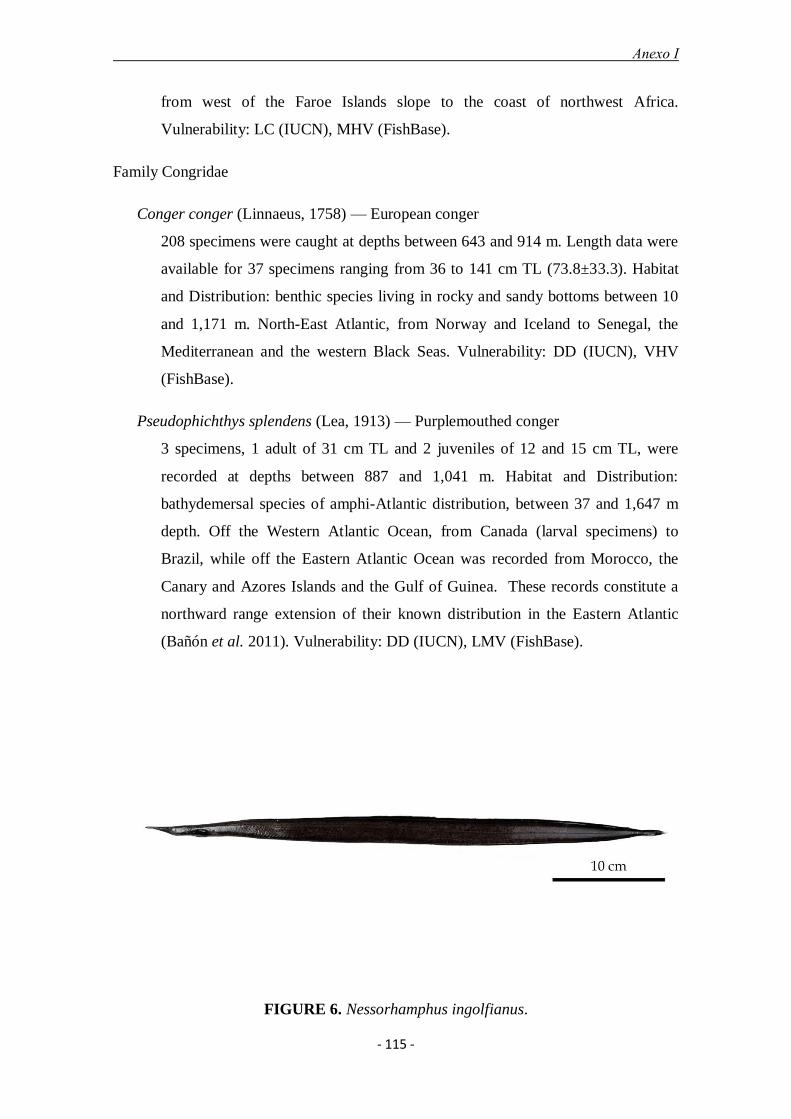
Anexo I
- 115 -
from west of the Faroe Islands slope to the coast of northwest Africa.
Vulnerability: LC (IUCN), MHV (FishBase).
Family Congridae
Conger conger (Linnaeus, 1758) — European conger
208 specimens were caught at depths between 643 and 914 m. Length data were
available for 37 specimens ranging from 36 to 141 cm TL (73.8±33.3). Habitat
and Distribution: benthic species living in rocky and sandy bottoms between 10
and 1,171 m. North-East Atlantic, from Norway and Iceland to Senegal, the
Mediterranean and the western Black Seas. Vulnerability: DD (IUCN), VHV
(FishBase).
Pseudophichthys splendens (Lea, 1913) — Purplemouthed conger
3 specimens, 1 adult of 31 cm TL and 2 juveniles of 12 and 15 cm TL, were
recorded at depths between 887 and 1,041 m. Habitat and Distribution:
bathydemersal species of amphi-Atlantic distribution, between 37 and 1,647 m
depth. Off the Western Atlantic Ocean, from Canada (larval specimens) to
Brazil, while off the Eastern Atlantic Ocean was recorded from Morocco, the
Canary and Azores Islands and the Gulf of Guinea. These records constitute a
northward range extension of their known distribution in the Eastern Atlantic
(Bañón et al. 2011). Vulnerability: DD (IUCN), LMV (FishBase).
FIGURE 6. Nessorhamphus ingolfianus.
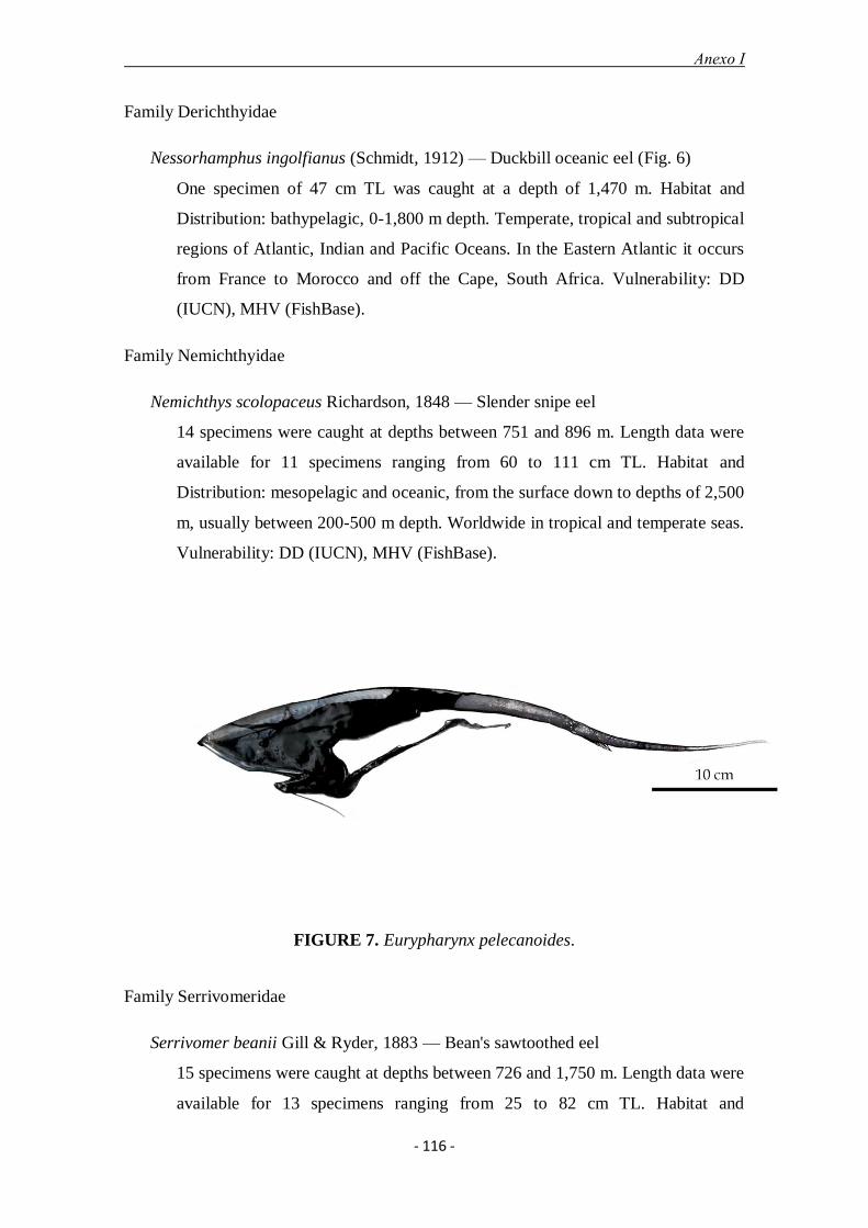
Anexo I
- 116 -
Family Derichthyidae
Nessorhamphus ingolfianus (Schmidt, 1912) — Duckbill oceanic eel (Fig. 6)
One specimen of 47 cm TL was caught at a depth of 1,470 m. Habitat and
Distribution: bathypelagic, 0-1,800 m depth. Temperate, tropical and subtropical
regions of Atlantic, Indian and Pacific Oceans. In the Eastern Atlantic it occurs
from France to Morocco and off the Cape, South Africa. Vulnerability: DD
(IUCN), MHV (FishBase).
Family Nemichthyidae
Nemichthys scolopaceus Richardson, 1848 — Slender snipe eel
14 specimens were caught at depths between 751 and 896 m. Length data were
available for 11 specimens ranging from 60 to 111 cm TL. Habitat and
Distribution: mesopelagic and oceanic, from the surface down to depths of 2,500
m, usually between 200-500 m depth. Worldwide in tropical and temperate seas.
Vulnerability: DD (IUCN), MHV (FishBase).
FIGURE 7. Eurypharynx pelecanoides.
Family Serrivomeridae
Serrivomer beanii Gill & Ryder, 1883 — Bean's sawtoothed eel
15 specimens were caught at depths between 726 and 1,750 m. Length data were
available for 13 specimens ranging from 25 to 82 cm TL. Habitat and

Anexo I
- 117 -
Distribution: epibenthic-pelagic species distributed in the Atlantic and western
Pacific Oceans. In the Eastern Atlantic it occurs from north to Iceland to South
Africa. Vulnerability: DD (IUCN), MV (FishBase).
ORDER SACCOPHARYNGIFORMES
Family Eurypharyngidae
Eurypharynx pelecanoides Vaillant, 1882 — Pelican eel (Fig. 7)
3 specimens between 34 and 47 cm TL were caught at depths between 780-
1,674 m. Habitat and Distribution: meso- to abyssopelagic and bathypelagic.
Circumglobal in tropical and temperate waters. In the Atlantic Ocean it is
recorded from off Iceland (65ºN) to 48ºS. Vulnerability: DD (IUCN), MHV
(FishBase).
ORDER OSMERIFORMES
FIGURE 8. Bathylagus euryops.
Family Bathylagidae
Bathylagus euryops Goode & Bean, 1896 — Goiter blacksmelt (Fig. 8)
2 specimens of 19 and 20 cm TL were caught at depths between 1,685 and 1,750
m. Habitat and Distribution: meso-and bathy pelagic zones of the North Atlantic,
sometimes in large aggregations, between 300 and 2,300 m depth. Western
Anexo I
- 118 -
Atlantic, as far north as Greenland, extending south to Bermuda and Eastern
Atlantic, from Iceland to Portugal. Vulnerability: DD (IUCN), LMV (FishBase).
Family Alepocephalidae
Alepocephalus rostratus Risso, 1820 — Risso's smooth-head
72 specimens were caught at depths between 781 and 1,683 m. Length data were
available for 51 specimens ranging from 18 to 65 cm TL (43.7±13.2). Habitat
and Distribution: bathydemersal, over soft bottoms at about 300-3,600 m depth,
usually at 300-1,600 m. Eastern Atlantic Ocean, from Iceland to Namibia and
Western Mediterranean Sea. Vulnerability: DD (IUCN), HHV (FishBase).
Alepocephalus bairdii Goode & Bean, 1879 — Baird's smooth-head
1,895 specimens were caught at depths between 711 and 1,809 m. Length data
were available for 1,228 specimens ranging from 13 to 89 cm TL (64.4±12.1).
Biometry and meristic: 6 specimens 521-817 mm TL, 443-708 mm SL; HL:
23.8-28.3; PO: 4.5-5.1; POL: 14.4-17.4; ED: 4.6-7.0; IOW: 3.4-4.4; PD: 55.6-
66.4; LD: 12.4-15.4; PA: 56.1-68.9; LA: 13.8-17.2, PP: 24.6-29.9; PV: 40.6-
49.2; LP: 7.7-11.5; LV: 4.9-5.6; H: 17.8-20.5; D: 20-22; A: 21-24; P: 10-13; V:
8-9; Gr: 8-11+1+18-19; SLL: 61-64. Habitat and Distribution: bathydemersal
over ooze and sand bottoms at a depth range of 365-2,500 m. Eastern Atlantic
Ocean, from Greenland and Iceland southward to 17°N and Western Atlantic
Ocean, from Greenland to Grand Banks and 29°52'N, 77°09'W. Vulnerability:
DD (IUCN), HHV (FishBase).
Xenodermichthys copei (Gill, 1884) — Bluntsnout smooth-head
69 specimens were caught at depths between 735 and 1,640 m. Length data were
available for 49 specimens ranging from 6 to 19 cm TL (14±2.8). Habitat and
Distribution: mesopelagic to benthopelagic as adults, between 100-2,650 m,
usually at 100-1,230 m depth. Widely distributed in the Atlantic, Eastern Pacific
and Indian Oceans. Vulnerability: DD (IUCN), MV (FishBase).
Rouleina attrita (Vaillant, 1888) — Softskin smooth-head
248 specimens were caught at depths between 1,470 and 1,809 m. Length data
were available for all specimens, ranging from 6 to 49 cm TL (25.4±9.6).
Habitat and Distribution: bathypelagic at depth range 450-2,300 m.
Anexo I
- 119 -
Circumglobal, widely distributed in the Atlantic, most Indian submarine ridges,
Subantarctic, North Pacific and tropical Western and Eastern Pacific Oceans.
Vulnerability: DD (IUCN), MHV (FishBase).
Conocara macropterum (Vaillant, 1888) — Longfin smooth-head
41 specimens were caught at depths between 1,674 and 1,809 m. Length data
were available for all specimens ranging from 17 to 39 cm TL (30.7±4.7).
Habitat and Distribution: epibenthic at about 800-2,677 m depth, usually at
1,200-1,800 m. Known from widely scattered localities on both sides of the
Atlantic Ocean, in Eastern Atlantic from 54°N to 45°S and in Western Atlantic
in Bahamas, Gulf of Mexico and off Brazil. Vulnerability: DD (IUCN), MHV
(FishBase).
ORDER STOMIIFORMES
Family Gonostomatidae
Gonostoma elongatum Günther, 1878 — Elongated bristlemouth fish
8 specimens were caught at depths between 740 and 916 m. Length data were
available for 4 specimens ranging from 18 to 24 cm TL. Habitat and
Distribution: meso- to bathypelagic, depth range 0-4,740 m, usually between
100-200 m and 500-800 m at night and 25-600 m and 1,250-1,500 m during the
day. Worldwide distribution, in tropical and subtropical Atlantic, Indian and
Pacific Oceans. In the Eastern Atlantic, from off Eastern Greenland, Iceland and
Spain south to the Gulf of Guinea, being more common south of 40°N.
Vulnerability: DD (IUCN), MV (FishBase).
Sigmops bathyphilus (Vaillant, 1884) — Spark anglemouth
3 specimens between 10 and 12 cm TL were caught at depths between 1,536 and
1,809 m. Habitat and Distribution: bathypelagic, juveniles and adults at 700-
3,000 m with marked stratification of size with depth. Temperate and subtropical
latitudes of the Atlantic, Pacific and Eastern Indian Oceans. Scattered records
from 65°'N to Namibia and South Africa in the Eastern Atlantic. Vulnerability:
DD (IUCN), MV (FishBase).
Cyclothone pallida Brauer, 1902 — Tan bristlemouth
Anexo I
- 120 -
1 specimen of 6 cm TL was caught at a depth of 1,674 m. Habitat and
Distribution: oceanic, meso- to bathypelagic, at a depth range of 16-4,663 m,
usually 600-1,800 m. Worldwide distribution, in tropical and subtropical
Atlantic, Indian and Pacific Oceans. Vulnerability: DD (IUCN), MV (FishBase).
Family Sternoptychidae
FIGURE 9. Sternoptyx diaphana.
Sternoptyx diaphana Hermann, 1781 — Diaphanous hatchet fish (Fig. 9)
One specimen of 4 cm TL was caught at a depth of 771 m. Habitat and
Distribution: bathypelagic, oceanodromous at depth range 400-3,676 m, usually
500-800 m. Mainly in tropical regions of Atlantic, Pacific and Indian Oceans.
Scattered records southwest of Ireland and also from Spain to Angola in the
Eastern Atlantic. Vulnerability: DD (IUCN), LV (FishBase).
Argyropelecus hemigymnus Cocco, 1829 — Half-naked hatchetfish
23 specimens were caught at depths between 765 and 1,460 m. Length data were
available for 22 specimens ranging from 2 to 4 cm TL. Habitat and Distribution:
oceanic and mesopelagic, from 100 to 4,054 m depth, mainly at 250-650 m.

Anexo I
- 121 -
Worldwide distribution in tropical and subtropical waters of all oceans.
Vulnerability: LC (IUCN), LV (FishBase).
Argyropelecus olfersii (Cuvier, 1829) — No common name
5 specimens were caught at depths between 771 and 1,674 m. Length data were
available for 4 specimens ranging from 9 to 11 cm TL. Habitat and Distribution:
oceanic, mesopelagic with adults and juveniles at 200-800 m during daylight
and from 100 (sometimes shallower) to 600 m at night. Restricted in the North-
East Atlantic Ocean between 35°N and 65°N, probably with a bipolar
distribution, and in the Southern Pacific Ocean between 30˚ S and 50˚S from
Chile to New Zealand. Vulnerability: DD (IUCN), LV (FishBase).
Argyropelecus aculeatus Valenciennes, 1850 — Lovely hatchetfish
1 specimen of 8 cm TL was caught at a depth of 791m. Habitat and Distribution:
oceanic and mesopelagic species at 100-600 m depth, concentrated at 300-600 m
during daylight and 100-300 at night. Atlantic Ocean, essentially absent from the
tropical Atlantic; Pacific from north of New Guinea to Japan and off eastern
Australia and Chile and central Indian Ocean from about 10°S to 40°S.
Vulnerability: DD (IUCN), LMV (FishBase).
Argyropelecus gigas Norman, 1930 — Hatchetfish
124 specimens between 6-11 cm TL were caught by bottom trawl during 1998's
surveys. They were identified as A. gigas, but we consider this identification, at
least in part, as dubious. The size of the specimens, which is larger in A gigas,
was used in the first surveys as one important criterion to differentiate
Argyropelecus species. However, in posterior surveys, we found a similar size
range in A. olfersii. Habitat and Distribution: bathypelagic at depth range 300-
1,000 m, usually 400-600 m. Circumglobal, except North-Eastern Pacific Ocean.
Vulnerability: DD (IUCN), LMV (FishBase).
Maurolicus muelleri (Gmelin, 1789) — Pearlsides
1 specimen of 5 cm TL was caught at a depth of 1,094 m. Habitat and
Distribution: mesopelagic, abundant near continental shelf-slope breaks and
seamounts and rare in the open ocean. It was found to depths of at least 1,524 m,
migrating in the water column at depths of 150-250 m during daylight and to
about 50 m at night. Tropical, subtropical, subarctic, and subantarctic waters of
Anexo I
- 122 -
the Pacific and Atlantic Oceans and the Mediterranean Sea. In the Eastern
Atlantic it occurs from Iceland and Norway to Senegal and also from
Democratic Republic of the Congo to Namibia. Vulnerability: DD (IUCN), LV
(FishBase).
FIGURE 10. Valenciennellus tripunctulatus.
Valenciennellus tripunctulatus (Esmark, 1871) — Constellationfish (Fig. 10)
1 specimen was caught at 790 m depth. Biometry and meristic: 34 mm TL, 29
mm SL. Photophores: VAV: 5; PV: 15; OA: 4; AC: 3+3+3+2+4; IP: 3+4.
Habitat and Distribution: oceanic and mesopelagic, between 100 and 700 m
depth, with marked stratification of size with depth. Worldwide in tropical and
temperate waters. Scattered records from the eastern Atlantic, in Iceland,
Ireland, and from Portugal to Namibia and in the Mediterranean Sea.
Vulnerability: DD (IUCN), LV (FishBase).
Family Phosichthyidae
Polymetme corythaeola (Alcock, 1898) — Rendezvous fish
124 specimens were caught at depths between 720 and 896 m. Length data were
available for 82 specimens ranging from 10 to 21 cm TL (16.8±2.7). Habitat and
Distribution: benthopelagic off continental and island slopes and seamounts in
the Atlantic, Eastern Pacific and Indo-West Pacific Oceans. Vulnerability: DD
(IUCN), LV (FishBase).

Anexo I
- 123 -
Family Stomiidae
Stomias boa (Risso, 1810) — Scaly dragonfish
7 specimens were caught at depths between 728 and 914 m. Length data were
available for 5 specimens ranging from 18 to 35 cm TL. Habitat and
Distribution: meso- to bathypelagic at depth range 200-1,500 m, but may
migrate to near-surface waters at night. Atlantic, Southeast Pacific and sub-
Antarctic region of the Indian Oceans and Western Mediterranean Sea.
Vulnerability: DD (IUCN), MV (FishBase).
Chauliodus sloani Bloch & Schneider, 1801 — Sloane's viperfish
56 specimens were caught at depths between 715 and 1,685 m. Length data were
available for 42 specimens ranging from 6 to 35 cm TL (23.3±7.1). Habitat and
Distribution: bathypelagic, depth range 400-2,800 m. Cosmopolitan in temperate
and tropical zones of all oceans, from about 63° N to 50° S and in the
Mediterranean Sea. Vulnerability: DD (IUCN), MV (FishBase).
FIGURE 11. Photostomias guernei.
Photostomias guernei Collett, 1889 — Loosejaw (Fig. 11)
4 specimens were caught at depths between 847 and 866 m. Length data were
available for 3 specimens ranging from 10 to 12 cm TL. Biometry and meristic:
Anexo I
- 124 -
107 mm TL, 99 mm SL; HL: 18.2; PO: 3.0; POL: 13.1; ED: 2.0; IOL: 4.0; PD:
84.8; LD: 12.1; PA: 83.8; LA: 13.1; PV: 46.5; LV: 42.4; H: 12.1; D: 22;A: 27.
Photophores: OA: 37; IC: 55. Habitat and Distribution: mesopelagic during
daylight to epipelagic at night, at depth range 1,138–3,100 m. Amphiatlantic, in
temperate and northern subtropical waters of the North Atlantic. Kenaley &
Hartel (2005) reported this species south to 3º58'N in the Eastern Atlantic, but
Quéro et al. (2003) recorded this species in Portugal and south of Spain. The
specimens captured in the Galicia Bank could constitute a new northern limit for
this specie in the Eastern Atlantic. Vulnerability: DD (IUCN), LV (FishBase).
Melanostomias bartonbeani Parr, 1927 — Scaleless black dragonfish
1 specimen was caught at a depth of 877 m. Biometry and meristic: 187 mm TL,
169 mm SL; HL: 14.2; BL: 18.9; H: 9.5; D: 13;A: 18; P: 5; V: 7. Photophores:
PV: 24. Habitat and Distribution: Meso- to bathypelagic at depth range 25-2,000
m. Nearly cosmopolitan in tropical and subtropical oceanic waters, apparently
absent from the Eastern Indian and Western Central Pacific Oceans. In the
Eastern Atlantic from 56°N to south of Guinea Bissau and also from Namibia to
South Africa. Vulnerability: DD (IUCN), MV (FishBase).
Flagellostomias boureei (Zugmayer, 1913) — Longbarb dragonfish
1 specimen was caught at depths between 768 and 786 m. Biometry and
meristic: 216 mm TL; 208 mm SL; HL: 13.0; PO: 4.3; POL: 5.8; ED: 2.9; IOL:
2.9; BL: 29.8 (broken); PD: 87.5; LD: 8.2; PA: 83.7; LA: 13.9; PV: 13.5; PD:
83.7; LV: 13.5; LP: H: 9.6; D: 13;A: 28; P: 10; V: 12. Habitat and Distribution:
meso- to bathypelagic at depth range 0-3,000 m. Circumglobal in tropical
through temperate seas. In the Eastern Atlantic from 58ºN to 40° S.
Vulnerability: DD (IUCN), MV (FishBase).
Malacosteus niger Ayres, 1848 — Stoplight loosejaw
6 specimens were caught at depths between 739 and 1,683 m. Length data were
available for 3 specimens ranging from 12 to 15 cm TL. Biometry and meristic:
140 mm TL; 130 mm SL; HL: 30.0; PO: 3.1; POL: 22.3; ED: 4.6; PD: 79.2; LD:
14.6; PA: 80.8; LA: 14.6; H: 17.7; D: 17; A: 19; P: 3; V: 6. Habitat and
Distribution: meso- to bathypelagic at depth range 500-3,886 m, usually 915-
1,830 m. It has been suggested that this species does not undergo substantial diel
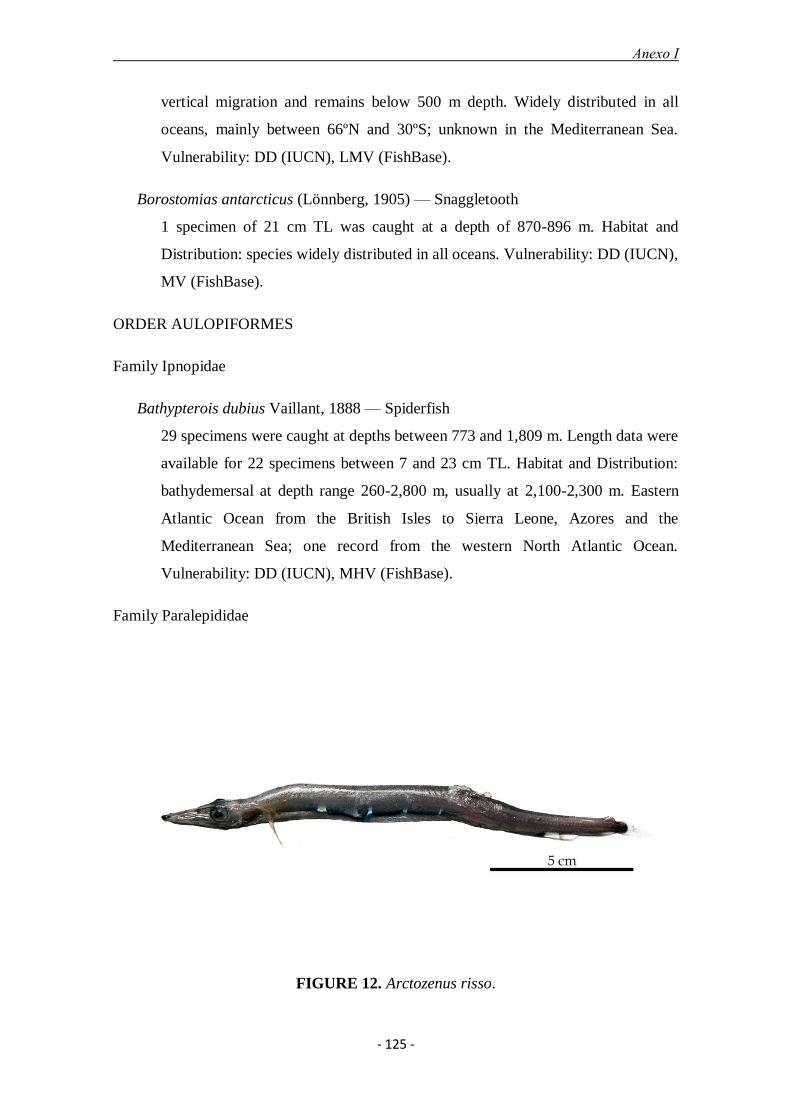
Anexo I
- 125 -
vertical migration and remains below 500 m depth. Widely distributed in all
oceans, mainly between 66ºN and 30ºS; unknown in the Mediterranean Sea.
Vulnerability: DD (IUCN), LMV (FishBase).
Borostomias antarcticus (Lönnberg, 1905) — Snaggletooth
1 specimen of 21 cm TL was caught at a depth of 870-896 m. Habitat and
Distribution: species widely distributed in all oceans. Vulnerability: DD (IUCN),
MV (FishBase).
ORDER AULOPIFORMES
Family Ipnopidae
Bathypterois dubius Vaillant, 1888 — Spiderfish
29 specimens were caught at depths between 773 and 1,809 m. Length data were
available for 22 specimens between 7 and 23 cm TL. Habitat and Distribution:
bathydemersal at depth range 260-2,800 m, usually at 2,100-2,300 m. Eastern
Atlantic Ocean from the British Isles to Sierra Leone, Azores and the
Mediterranean Sea; one record from the western North Atlantic Ocean.
Vulnerability: DD (IUCN), MHV (FishBase).
Family Paralepididae
FIGURE 12. Arctozenus risso.
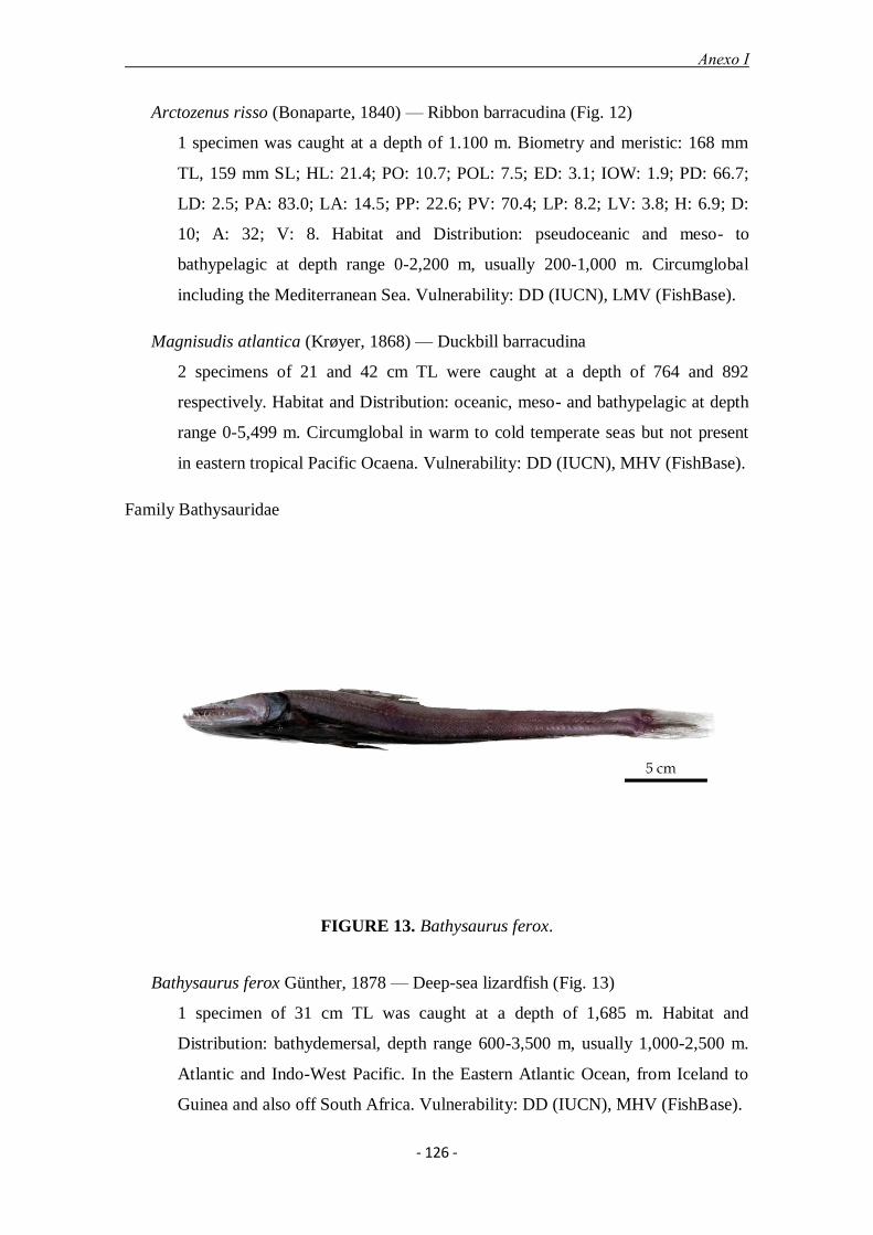
Anexo I
- 126 -
Arctozenus risso (Bonaparte, 1840) — Ribbon barracudina (Fig. 12)
1 specimen was caught at a depth of 1.100 m. Biometry and meristic: 168 mm
TL, 159 mm SL; HL: 21.4; PO: 10.7; POL: 7.5; ED: 3.1; IOW: 1.9; PD: 66.7;
LD: 2.5; PA: 83.0; LA: 14.5; PP: 22.6; PV: 70.4; LP: 8.2; LV: 3.8; H: 6.9; D:
10; A: 32; V: 8. Habitat and Distribution: pseudoceanic and meso- to
bathypelagic at depth range 0-2,200 m, usually 200-1,000 m. Circumglobal
including the Mediterranean Sea. Vulnerability: DD (IUCN), LMV (FishBase).
Magnisudis atlantica (Krøyer, 1868) — Duckbill barracudina
2 specimens of 21 and 42 cm TL were caught at a depth of 764 and 892
respectively. Habitat and Distribution: oceanic, meso- and bathypelagic at depth
range 0-5,499 m. Circumglobal in warm to cold temperate seas but not present
in eastern tropical Pacific Ocaena. Vulnerability: DD (IUCN), MHV (FishBase).
Family Bathysauridae
FIGURE 13. Bathysaurus ferox.
Bathysaurus ferox Günther, 1878 — Deep-sea lizardfish (Fig. 13)
1 specimen of 31 cm TL was caught at a depth of 1,685 m. Habitat and
Distribution: bathydemersal, depth range 600-3,500 m, usually 1,000-2,500 m.
Atlantic and Indo-West Pacific. In the Eastern Atlantic Ocean, from Iceland to
Guinea and also off South Africa. Vulnerability: DD (IUCN), MHV (FishBase).
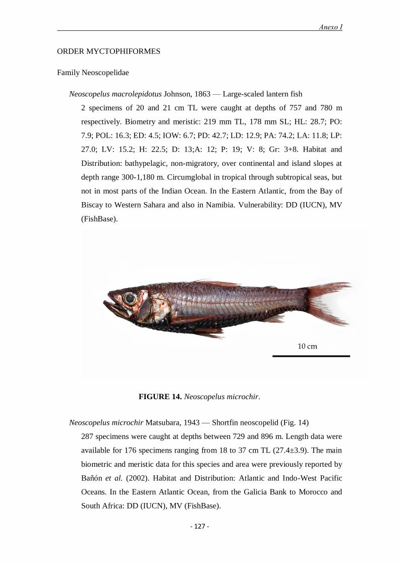
Anexo I
- 127 -
ORDER MYCTOPHIFORMES
Family Neoscopelidae
Neoscopelus macrolepidotus Johnson, 1863 — Large-scaled lantern fish
2 specimens of 20 and 21 cm TL were caught at depths of 757 and 780 m
respectively. Biometry and meristic: 219 mm TL, 178 mm SL; HL: 28.7; PO:
7.9; POL: 16.3; ED: 4.5; IOW: 6.7; PD: 42.7; LD: 12.9; PA: 74.2; LA: 11.8; LP:
27.0; LV: 15.2; H: 22.5; D: 13;A: 12; P: 19; V: 8; Gr: 3+8. Habitat and
Distribution: bathypelagic, non-migratory, over continental and island slopes at
depth range 300-1,180 m. Circumglobal in tropical through subtropical seas, but
not in most parts of the Indian Ocean. In the Eastern Atlantic, from the Bay of
Biscay to Western Sahara and also in Namibia. Vulnerability: DD (IUCN), MV
(FishBase).
FIGURE 14. Neoscopelus microchir.
Neoscopelus microchir Matsubara, 1943 — Shortfin neoscopelid (Fig. 14)
287 specimens were caught at depths between 729 and 896 m. Length data were
available for 176 specimens ranging from 18 to 37 cm TL (27.4±3.9). The main
biometric and meristic data for this species and area were previously reported by
Bañón et al. (2002). Habitat and Distribution: Atlantic and Indo-West Pacific
Oceans. In the Eastern Atlantic Ocean, from the Galicia Bank to Morocco and
South Africa: DD (IUCN), MV (FishBase).

Anexo I
- 128 -
Family Myctophidae
Myctophum punctatum Rafinesque, 1810 — Spotted lanternfish
1 specimen of 9 cm TL was caught at a depth of 749 m. Habitat and
Distribution: high-oceanic, mesopelagic at depth range 0-1,000 m;
nyctoepipelagic at the surface and down to 125 m and between 225-1,000 m
during the day. North Atlantic Ocean, from 69ºN to 15ºN and in the
Mediterranean Sea. Vulnerability: DD (IUCN), LMV (FishBase).
Benthosema glaciale (Reinhardt, 1837) — Glacier lantern fish
3 specimens were caught at depths between 790 and 796 m. Habitat and
Distribution: pelagic-oceanic, non-migratory, at depth range 0-1,407 m, usually
300-400 m. North Atlantic Ocean, between 81°N - 11°N and 76°W - 29°E. In
the Eastern Atlantic Ocean, from Greenland to Guinea and in the Mediterranean
Sea. Vulnerability: DD (IUCN), LMV (FishBase).
FIGURE 15. Electrona rissoi.
Ceratoscopelus maderensis (Lowe, 1839) — No common name
1 specimen of 8 cm TL was caught at 1,079 m depth. Habitat and Distribution:
mesopelagic and high-oceanic species, between 12-1,500 m depth, 650-700 m
during the day and between 51-250 m at night. Temperate-subtropical Atlantic
Ocean and in the Mediterranean Sea. In the eastern Atlantic Ocean, from about

Anexo I
- 129 -
57° N to the Mauritanian upwelling area. Vulnerability: DD (IUCN), LMV
(FishBase).
Electrona rissoi (Cocco, 1829) — Electric lantern fish (Fig. 15)
2 specimens of 6 and 7 cm TL were caught at a depth of 762 and 782 m
respectively. Biometry and meristic: 62 mm TL, 57 mm SL; HL: 36.8; PO: 7.0;
POL: 15.8; ED: 14.0; IOW: 5.3; PD: 50.9; LD: 15.8; PA: 63.2; LA: 26.3, LP:
24.6; LV: 15.8; H: 29.8; D: 13; A: 19; P: 16; V: 9; Gr: 9+19. Photophores: PVO:
2; PLO: 1; PO: 5; VLO: 1; SAO: 3;VO: 4; AO: 11. Habitat and Distribution:
high-oceanic and mesopelagic. Disjunct, circumtropical, in warm latitudes of
Atlantic, Indian and Pacific Oceans and in the Mediterranean Sea. Vulnerability:
DD (IUCN), LV (FishBase).
Lampadena speculigera Goode & Bean, 1896 — Mirror lanternfish
1 specimen of 10 cm TL was caught at depths between 755 and 759 m. Habitat
and Distribution: oceanic and mesopelagic, depth range 0-1,000 m, between
475-950 m during the day and between 60-750 m at night. North Atlantic Ocean
and southern circumglobal, between 66°N - 48°S. Vulnerability: DD (IUCN),
MV (FishBase).
Notoscopelus kroeyeri (Malm, 1861) — Lancet fish
3 specimens between 12 and 14 cm TL were caught at depths between 749 and
766 m. Habitat and Distribution: epi- to bathypelagic and high-oceanic, from
325 to deeper than 1,000 m during the day and at surface and down to 125 m
during the night. North Atlantic Ocean, between the Arctic Circle and 37°N in
the east and between 60°N and 40°N in the west. Vulnerability: DD (IUCN),
MV (FishBase).
ORDER GADIFORMES
Family Macrouridae
Trachyrincus scabrus (Rafinesque, 1810) — Roughsnout grenadier
69 specimens were caught at depths between 711 and 1,101 m. Length data were
available for 17 specimens ranging from 2.5 to 20 cm PAL. Habitat and
Distribution: bathydemersal at depth range 300-1,700 m. North Atlantic Ocean

Anexo I
- 130 -
and the Mediterranean Sea. In the eastern Atlantic, from Scotland to South
Africa. Vulnerability: DD (IUCN), LMV (FishBase).
Hymenocephalus italicus Giglioli, 1884 — Glasshead grenadier
56 specimens were caught at depths between 731 and 868 m. Length data were
available for 16 specimens ranging from 3 to 5.5 cm PAL. Habitat and
Distribution: benthopelagic at depth range 100-1,400 m. Atlantic and Western
Indian Oceans and in the Mediterranean Sea. In the eastern Atlantic Ocean, from
the Gulf of Biscay to Angola and South Africa. Vulnerability: DD (IUCN),
LMV (FishBase).
Coelorinchus caelorinchus (Risso, 1810) — Hollowsnout grenadier
9 specimens were caught at depths between 749 and 1,041 m. Length data were
available for 7 specimens ranging from 1 to 10 cm PAL. Habitat and
Distribution: benthopelagic at depth range 90-1,250 m, usually 200-500. North
Atlantic Ocean and the Mediterranean Sea. In the eastern Atlantic Ocean, from
Iceland and Faroe islands to Mauritania. Vulnerability: DD (IUCN), HV
(FishBase).
Coelorinchus labiatus (Koelher, 1896) — Spearsnouted grenadier
117 specimens were caught at depths between 1,094 and 1,809 m. Length data
were available for 117 specimens ranging from 8.5 to 18 cm PAL (12.3±2.2).
Habitat and Distribution: bathydemersal at depth range 460-2,220 m. North
Atlantic Ocean and the Mediterranean Sea. In the eastern Atlantic, from Iceland
to Mauritania. Vulnerability: DD (IUCN), MHV (FishBase).
Coryphaenoides rupestris Gunnerus, 1765 — Roundhead rat-tail
34 specimens were caught at depths between 720 and 1,536 m. Length data were
available for 13 specimens ranging from 5 to 13 cm PAL. Habitat and
Distribution: bathypelagic at depth range 180-2,600 m, in continental, island,
and seamount slopes. North Atlantic Ocean, from Iceland and Norway to
western Sahara in the eastern Atlantic Ocean. Vulnerability: EN (IUCN), HHV
(FishBase).
Coryphaenoides guentheri (Vaillant, 1888) — Günther's grenadier

Anexo I
- 131 -
40 specimens were caught at depths between 1,470 and 1,809 m. Length data
were available for 40 specimens ranging from 3 to 13 cm PAL (8.1±2.1).
Biometry and meristic: 320 mm TL, 316 mm SL; HL: 16.5; PO: 4.4; POL: 7.6;
ED: 4.4; IOW: 3.8; BL: 1.6; PD1: 20.3; PD2: 34.8; LD1: 4.7; LD2: 65.2; PA:
28.2; LA: 71.8; PP: 19.3; PV: 19.6; LP: 12.3; LV: 8.2; H: 12.7; D1: II+9; P: 22;
V: 7; Gr: 2+6. Habitat and Distribution: bathydemersal at depth range 831-2,830
m. North Atlantic Ocean and Mediterranean Sea. In the eastern Atlantic Ocean,
from Iceland and Denmark Strait to Mauritania and Gabon. Vulnerability: DD
(IUCN), MHV (FishBase).
Coryphaenoides mediterraneus (Giglioli, 1893) — Mediterranean grenadier
10 specimens were caught at depths between 1,470 and 1,809 m. Length data
were available for all specimens ranging from 3.5 to 17.5 cm PAL. Habitat and
Distribution: bathypelagic at depth range 883-4,262 m. North Atlantic Ocean
and in the Mediterranean Sea. In the eastern Atlantic Ocean, from Iceland and
west Scotland to Mauritania. Vulnerability: DD (IUCN), HV (FishBase).
Malacocephalus laevis (Lowe, 1843) — Rough rat-tail
924 specimens were caught at depths between 709 and 916 m. Length data were
available for 378 specimens ranging from 3 to 12 cm PAL (6.7±1.7). Habitat and
Distribution: bathydemersal at depth range 200-1,000 m, usually 300-750 m.
Atlantic and Indo-west-central Pacific Oceans. In the eastern Atlantic Ocean,
from Iceland and Faroe islands to South Africa. Vulnerability: DD (IUCN), HV
(FishBase).
Nezumia aequalis (Günther, 1878) — Common Atlantic grenadier
3,645 specimens were caught at depths between 737 and 1,470 m. Length data
were available for 544 specimens ranging from 1 to 9 cm PAL (4.3±1.3). Habitat
and Distribution: benthopelagic at depth range 200-2,320 m, usually 200-1,000
m. North Atlantic Ocean and the Mediterranean Sea. In the eastern Atlantic,
from the Faroe Bank Channel to northern Angola. Vulnerability: DD (IUCN),
MV (FishBase).
Family Bathygadidae
Gadomus longifilis (Goode & Bean, 1885) — Treadfin grenadier

Anexo I
- 132 -
3 specimens ranging from 27 to 29 cm TL were caught at depths between 1,450
and 1,683 m (Bañón et al., 2013a). Habitat and Distribution: benthopelagic,
between 520 and 2,165 m depth. Amphi-Atlantic in tropical and subtropical
North Atlantic Ocean. In Western Atlantic, from Greenland to the Gulf of
Mexico and Caribbean Sea and from the northwest of Spain to the Gulf of
Guinea in the Eastern Atlantic. Vulnerability: DD (IUCN), MV (FishBase).
Gadomus dispar (Vaillant, 1888) — No common name
6 specimens ranging from 17 to 36 cm TL were caught at depths between 764
and 1,051 m (Bañón et al. 2013a). Habitat and Distribution: benthopelagic
between 548 and 1,543 m depth. Amphi-Atlantic distribution in tropical and
subtropical North Atlantic Ocean. In Western Atlantic, from Norfolk Canyon to
the Caribbean Sea and in Eastern Atlantic from the Cantabrian Sea to Mauritania
and Guinea-Bissau. Vulnerability: DD (IUCN), MHV (FishBase).
FIGURE 16. Guttigadus latifrons.
Bathygadus melanobranchus Vaillant, 1888 — Vaillant's grenadier
One specimen of 37 cm TL was caught at depths between 1,185 and 1,187 m
(Bañón et al. 2013a). Habitat and Distribution: benthopelagic at depths between
450 and 2,650 m, but generally from 700 to 1,400 m. Amphi-Atlantic
distribution, in tropical and subtropical latitudes. In the Eastern Atlantic, from

Anexo I
- 133 -
the Irish continental slope to Senegal and Gabon. Vulnerability: DD (IUCN),
MHV (FishBase).
Family Moridae
Guttigadus latifrons (Holt & Byrne, 1908) — No common name (Fig. 16)
4 specimens ranging 11-13 cm TL were caught at depths between 791 and 851
m. Biometry and meristic: 129 mm TL; 118 mm SL; HL: 23.7; PO: 5.1; POL:
11.0; ED: 7.6; IOW: 8.5; BL: 2.5; PD1: 24.6; PD2: 28.8; LD1: 3.4; LD2: 58.5;
PA: 29.7; LA: 58.5; LP: 15.3; LV: 22.0; H: 22.0; D1: 5;D2: 72; A: 68; P: 22; V:
3; Gr: 7+16. Habitat and Distribution: bathydemersal between 770-1,875 m
depth. Eastern and Southwestern Atlantic Ocean, Western Indian Ocean and in
the Mediterranean Sea. In the Eastern Atlantic, from Ireland and Island to the
Azores islands and the Galicia Bank. Vulnerability: DD (IUCN), MV
(FishBase).
Halargyreus johnsonii Günther, 1862 — Slender codling
207 specimens were caught at depths between 731 and 1,685 m. Length data
were available for 137 specimens ranging from 9 to 45 cm TL (29.7±9.6).
Habitat and Distribution: bathypelagic, antitropical at depth range 450-3,000 m.
North Atlantic, South Atlantic, South-west Pacific, and South-east Pacific
Oceans. Patchy distribution in subarctic and subantarctic waters. Vulnerability:
DD (IUCN), HV (FishBase).
Physiculus dalwigki Kaup, 1858 — Black codling
One specimen of 26 cm TL was caught at depths between 731-738m m (Bañón
et al. 2002). Habitat and Distribution: benthopelagic at depth range 100-738 m.
Eastern Atlantic: Galicia Bank, Great Meteor Bank, Madeira and south along the
African coast to about 25°N and in Western Mediterranean Sea. Vulnerability:
DD (IUCN), MV (FishBase).
Mora moro (Risso, 1810) — Common mora
6,596 specimens were caught at depths between 709 and 1,323 m. Length data
were available for 1,310 specimens ranging from 13 to 67 cm TL (47.9 ±9.3),
with males between 25 and 55 cm (45.7 ±4.0, N=431) and females between 35
and 65 cm (54.8 ±4.5, N=490). Habitat and Distribution: bathypelagic; depth

Anexo I
- 134 -
range 400-2,500 usually 400-1,000 m. Wide distribution along the Atlantic,
Pacific and Indian Oceans and in the Western Mediterranean Sea. In the Eastern
Atlantic, from Iceland and Faeroes to Cape Bojador, West Africa, and including
Azores Islands and Madeira archipelago. Vulnerability: DD (IUCN), HV
(FishBase).
Lepidion lepidion (Risso, 1810) — Mediterranean codling
41,585 specimens were caught at depths between 709 and 1,323 m. Length data
were available for 3,196 specimens ranging from 11 to 53 cm TL (26±5.2).
Following a recent revision of the genus, the Atlantic L. eques has been
proposed as a junior synonym of the Mediterranean L. lepidion (Bañón et al.
2013b). Habitat and Distribution: benthopelagic, depth range 127-1,880 m,
usually 500-900 m. North Atlantic Ocean and the Mediterranean Sea.
Vulnerability: LC (IUCN), MHV (FishBase).
FIGURE 17. Lepidion guentheri.
Lepidion guentheri (Giglioli, 1880) — No common name (Fig. 17)
One specimen was caught at a depth of 1,536 m. Biometry and meristic: 697
mm TL; 632 mm SL; HL: 22.2; PO: 5.7; POL: 12.3; ED: 4.1; IOW: 5.1;
PD1:25.3; PD2: 29.3; LD1: 2.5; LD2: 62.8; PA: 48.3; LA: 62.8, PV: 19.3; PP:
24.4; LP: 13.9; LV: 30.4; H: 23.1; 1D: 5; 2D: 56; P: 21; V: 6; A:50; Gr: 6+16.
Habitat and Distribution: benthopelagic between 750 and 2,196 m depth. North-

Anexo I
- 135 -
eastern Atlantic, in west of Ireland, west and north coasts of Spain, north coast
of Portugal, the Azores, Madeira, Canary Islands and the Mid-Atlantic Ridge
and in Western Mediterranean Sea. Vulnerability: DD (IUCN), HHV
(FishBase).
Antimora rostrata (Günther, 1878) — Blue antimora
One specimen of 16 cm TL was caught at a depth of 1,750 m. Habitat and
Distribution: bathypelagic at depth range 350-3,000 m, usually 1,300-2,500 m.
Circumglobal, except North Pacific. In the Eastern Atlantic, from Iceland to
South Africa. Vulnerability: DD (IUCN), HHV (FishBase).
Family Melanonidae
Melanonus zugmayeri Norman, 1930 — Arrowtail
38 specimens were caught at depths between 773 and 1,470 m. Length data
were available for 28 specimens ranging from 13 to 28 cm TL. Habitat and
Distribution: oceanic and bathypelagic at depth range 0-3,000 m. Circumglobal
in tropical and subtropical seas. Vulnerability: DD (IUCN), LV (FishBase).
Family Gadidae
Micromesistius poutassou (Risso, 1827) — Blue whiting
165 specimens were caught at depths between 709 and 892 m. Length data were
available for 102 specimens ranging from 12 to 40 cm TL (29.2±4.7). Habitat
and Distribution: oceanic and bathypelagic at depth range 150-3,000 m, usually
300-400 m. Northeast Atlantic, from 26ºN to 82ºN, with smaller populations in
the Northwest Atlantic and the Mediterranean Sea. Vulnerability: DD (IUCN),
LMV (FishBase).
Family Lotidae
Gaidropsarus granti (Regan, 1903) — Azores rockling
2 specimens of 33 and 17 cm TL were caught at depths of 782 and 866 m
respectively (Bañón et al. 2002, 2010). Habitat and Distribution: demersal from
20 to over 800 m depth. Eastern Atlantic, in the Galicia Bank, Canary and the
Azores Islands and in the Eastern Mediterranean Sea. Vulnerability: DD
(IUCN), MV (FishBase).

Anexo I
- 136 -
Family Phycidae
Phycis blennoides (Brünnich, 1768) — Greater forkbeard
560 specimens were caught at depths between 709 and 952 m. Length data were
available for 111 specimens ranging from 20 to 79 cm TL (38.6±16.1). Habitat
and Distribution: benthopelagic over sandy and muddy bottoms at depth range
10-1,047 m, usually 100-450 m, with juveniles more coastal, over the
continental shelf while adults migrate along the slope. Eastern Atlantic, from
Norway and Iceland to Mauritania and in the Mediterranean Sea. Vulnerability:
DD (IUCN), HV (FishBase).
Family Merluccidae
Merluccius merluccius (Linnaeus, 1758) — European hake
One specimen, a female of 61 cm TL was caught at a depth of 795 m. Habitat
and Distribution: demersal to benthopelagic over sandy and muddy bottoms at
depth range 30-1,075 m, usually 50-370 m. Eastern Atlantic, from Norway and
Iceland to Mauritania and in the Mediterranean Sea. Vulnerability: DD (IUCN),
HV (FishBase).
ORDER OPHIDIIFORMES
FIGURE 18. Cataetyx alleni.

Anexo I
- 137 -
Family Bythitidae
Cataetyx alleni (Byrne, 1906) — No common name (Fig. 18)
29 specimens were caught at depths between 755 and 916 m. Length data were
available for 20 specimens ranging from 9 to 15 cm TL. Habitat and
Distribution: bathydemersal, depth range 480-1,851 m, usually below 600 m.
Eastern Atlantic, from the South-west Ireland to Portugal and Western
Mediterranean Sea. Vulnerability: DD (IUCN), LV (FishBase).
Cataetyx laticeps Koefoed, 1927 — No common name
2 specimens of 72 and 82 cm TL were caught at depths of 1,683 and 1,685 m
respectively. Habitat and Distribution: bathydemersal or benthopelagic at depth
range 500-2,830. North Atlantic Ocean and the Mediterranean Sea. In the
Eastern Atlantic, from Iceland, scattered localities around the British Isles,
France, Azores, and along the coast of West Africa to the Cape of Good Hope.
Vulnerability: DD (IUCN), HV (FishBase).
Family Ophididae
FIGURE 19. Spectrunculus grandis.
Spectrunculus grandis (Günther, 1877) — Pudgy cuskeel (Fig. 19)
One specimen of 55 cm TL was caught at a depth of 1,809 m. Habitat and
Distribution: bathydemersal; depth range 800-4,300 m, usually 2,000-3,000 m.

Anexo I
- 138 -
Widely distributed in all oceans, between 57°N and 59°S. Vulnerability: DD
(IUCN), HHV (FishBase).
ORDER LOPHIIFORMES
Family Lophiidae
Lophius piscatorius Linnaeus, 1758 — Anglerfish
137 specimens were caught at depths between 709 and 916 m. Length data were
available for 41 specimens ranging from 17 to 97 cm TL (75.8±14.8) with
males between 64 and 92 cm (N=8) and females between 67 and 97 cm (N=10).
Habitat and Distribution: bathydemersal on sandy, muddy, gravelly and
occasionally rocky bottoms, at depths from 20 to 2,600 m. Eastern Atlantic,
from Iceland and south-western Barents Sea to Mauritania, including the
Mediterranean and Black Sea. Vulnerability: DD (IUCN), HHV (FishBase).
Family Chaunacidae
Chaunax pictus Lowe, 1846 — Pink frogmouth
63 specimens were caught at depths between 726 and 940 m. Length data were
available for 40 specimens ranging from 12 to 41 cm TL (23.6±7.1). Habitat and
Distribution: bathydemersal on continental shelves, slopes and seamounts at
depth range 200-978 m. Circumglobal in tropical to temperate waters, although
Ho & Last (2013) limited its presence to the Atlantic Ocean. Vulnerability: DD
(IUCN), LMV (FishBase).
Family Linophrynidae
Linophryne coronata Parr, 1927 — Deep-sea anglerfish
One female of 223 mm TL with attached parasitic male of 29 mm TL was
caught at depths between 762 and 764 m (Bañón et al. 2006b). Habitat and
Distribution: meso- to bathypelagic, depth range 0-1,500 m. Scattered records in
the Atlantic and Eastern North Pacific Oceans. Vulnerability: DD (IUCN), LV
(FishBase).
ORDER BERYCIFORMES
Family Trachichthyidae
Anexo I
- 139 -
Hoplostethus mediterraneus Cuvier, 1829 — Mediterranean slimehead
61,206 specimens were caught at depths between 737 and 1,187 m. Length data
were available for 9,177 specimens ranging from 7 to 36 cm TL (21.5±3.4).
Habitat and Distribution: benthopelagic at depth range 100-1175 m, usually 500-
800 m. Northeastern Atlantic, Indian and South Pacific Oceans and in
Mediterranean Sea. In the Eastern Atlantic, from Ireland to South Africa.
Vulnerability: DD (IUCN), HV (FishBase).
Hoplostethus cadenati Quéro, 1974 — Black slimehead
47 specimens were caught between 777 and 940 m depth. Length data were
available for 22 specimens ranging from 20 to 29 cm TL. Biometry and meristic:
272 and 237 mm TL; 210 and 184 mm SL; HL: 38.1 and 38.6; PO: 9.0 and 10.9;
POL: 18.1 and 17.9; ED: 11.0 and 9.8; PD:41.9 and 41.8; LD: 37.1 and 38.0;
PA: 65.2 and 64.1; LA: 17.6 and 18.5, LP: 33.3 and 32.6; LV: 21.0 and 19.0; H:
41.4 and 44.6; D: VI+13 and V+14; A:III+10; P: 17; V: I+5 and I+6; Gr: 5+17.
Habitat and Distribution: bathypelagic, living near the bottom from 70 to at least
1,000 m depth, usually 200-700 m. Eastern Atlantic and Western Indian Oceans.
In the eastern Atlantic, from northwest Ireland, northwest Spain and along the
northwest coast of Africa between 27°30'N and 10°10'N and from 1°26'S to
26'14°S. Vulnerability: DD (IUCN), HV (FishBase).
Hoplostethus atlanticus Collett, 1889 — Orange roughy
3 specimens of 21, 24 and 31 cm TL were caught at depths between 1,470 and
1,685 m. Habitat and Distribution: bathypelagic, inhabits deep, cold waters over
steep continental slopes, ocean ridges and seamounts, sometimes in dense
aggregations, from 180 to 1,809 m depth, usually 400-900 m. Atlantic and Indo-
West Pacific Oceans but not in the eastern Pacific. In the Eastern Atlantic, from
Iceland to Morocco and from Namibia to South Africa. Vulnerability: VU
(IUCN, OSPAR), HHV (FishBase).
Family Diretmidae
Diretmichthys parini (Post & Quéro, 1981) — Parin's spiny fin (Fig. 20)
Two specimens were caught at depths between 780 and 1,315 m. Biometry and
meristic: 241 and 266 mm TL; 195 and 211 mm SL; HL: 35.9 and 36.5; PO: 6.7
and 9.5; POL: 15.9 and 11.4; ED: 13.3 and 16.1; IOW: 4.6 and 5.2; PD:42.1 and
Anexo I
- 140 -
43.1; LD: 42.1 and 43.1; PA: 60.0 and 61.6; LA: 42.1 and 32.2, LP: 27.2 and
27.5; LV: 28.7 and 29.9; H: 45.6 and 46.0; D: 27 and 29; P: I+17; V: I+6; A: 21
and 23; Gr: 6+1+12. Habitat and distribution: tropical, subtropical and moderate
latitudes of the Atlantic, Pacific and Indian Oceans at depths ranging from to
270 to more than 2000 m, with juveniles from epipelagic to mesopelagic zone
and adults collected close to the bottom (Arronte & Heredia 2006).
Vulnerability: DD (IUCN), LMV (FishBase).
FIGURE 20. Diretmichthys parini.
Diretmus argenteus Johnson, 1864 — Silver spinyfin
Five specimens were caught at depths between 777 and 940 m. Two specimens
were 6 and 26 cm TL respectively. Habitat and distribution: bathypelagic at
depth range 0-2,000 m, usually 500-700 m. Circumglobal in temperate and
tropical seas. In the Eastern Atlantic, from Iceland and British Isles to South
Africa including the Canary and Ascension Islands. Vulnerability: DD (IUCN),
LV (FishBase).
Family Berycidae
Beryx splendens Lowe, 1834 — Splendid alfonsino

Anexo I
- 141 -
1,968 specimens were caught at depths between 643 and 914 m. Length data
were available for 698 specimens ranging from 21 to 48 cm TL (36.5±4.4).
Habitat and Distribution: benthopelagic on continental shelves and slopes,
seamounts, and oceanic ridges in a depth range from 25 to 1,300 m, usually 200-
800 m. Circumglobal distribution, in temperate to tropical waters excluding the
North-eastern Pacific. In the Eastern Atlantic, from Ireland to South Africa.
Vulnerability: DD (IUCN), HV (FishBase).
Beryx decadactylus Cuvier, 1829 — Beryx
18 specimens were caught at depths between 643 and 877 m. Length data were
available for 11 specimens ranging from 44 to 58 cm TL. Length data available
during the exploratory surveys carried out in the 1980's was from 24 to 59 cm
TL, but the total number of individuals caught was not reported. Habitat and
Distribution: benthopelagic with a world-wide distribution, occurring in tropical,
subtropical and some temperate areas of the Atlantic, Pacific and Indian Oceans,
and in the Western Mediterranean Sea. In the Eastern Atlantic, from Greenland,
Iceland and Norway to Western Sahara and South Africa. Vulnerability: DD
(IUCN), HHV (FishBase).
Family Oreosomatidae
FIGURE 21. Neocyttus helgae.

Anexo I
- 142 -
Neocyttus helgae (Holt & Byrne, 1908) — False boarfish (Fig. 21)
One specimen was caught at depths between 1,410 and 1,427 m. Biometry and
meristic: 119 mm TL; 100 mm SL; HL: 35.0; PO: 9.0; POL: 7.0; ED: 19.0;
IOW: 12.0; PD: 45.0; LD: 50.0; PA: 48.0; LA: 37.0; PP: 40.0; PV: 39.0; LP:
15.0; LV: 15.0; H: 51.0; D: VII+33; A: IV+31; P: 19; V: I+6; Gr: 5+18; SLL:
80. Habitat and Distribution: bathypelagic species along the outer continental
shelf insular slope and seamounts, strongly associated with habitats of high
currents, ripple marks, slopes, reefs of rocks and gorgonians, at depths from 850
to 1,700 m. Northeast Atlantic, from Iceland to Madeira and Western North
Atlantic. Vulnerability: DD (IUCN), HV (FishBase).
ORDER SYNGNATHIFORMES
Family Syngnathidae
Entelurus aequoreus (Linnaeus, 1758) — Snake pipefish
34 specimens between 11 and 35 cm TL were caught over seabed depths of 766-
866 m, probably during the hauling of the bottom trawl. Habitat and
Distribution: coastal or oceanic pelagic species. Eastern Atlantic Ocean, from
the Azores to Iceland and Norway, including the Baltic Sea. Vulnerability: DD
(IUCN), LMV (FishBase).
ORDER SCORPAENIFORMES
Family Sebastidae
Helicolenus dactylopterus (Delaroche, 1809) — Blackbelly rosefish
2 specimens were caught at depths between 704 and 869 m. Only one individual
of 37 cm TL was measured. Habitat and Distribution: bathydemersal in soft
bottom areas of the continental shelf and upper slope, at depth range 50-1,100
m, usually 150-600 m. Western Atlantic, from Canada to Venezuela and Eastern
Atlantic, from Iceland and Norway to South Africa and in the Mediterranean
Sea. Vulnerability: DD (IUCN), MHV (FishBase).
Anexo I
- 143 -
Trachyscorpia cristulata echinata (Koehler, 1896) — Spiny scorpionfish
1,105 specimens were caught at depths between 709 and 1,323 m. Length data
were available for 267 specimens ranging from 12 to 50 cm TL (37.4±8.7).
Biometry and meristic: 4 specimens, 392-506 mm TL, 336-418 mm SL; HL:
43.6-47.1; PO: 11.2-14.4; POL: 23.2-24.5; ED: 8.9-10.1; IOW: 4.7-5.5; PD:
33.5-41.1; LD: 46.7-50.3; PA: 68.7-74.2; LA: 11.2-13.2; PP: 42.9-44.3; PV:
39.3-41.8; LP: 21.3-24.9; LV: 14.4-17.6; H: 29.9-32.5; D: XII+9; A: III+5; P:
20-21; V: I+5; Gr: 6+12-13. Habitat and Distribution: bathydemersal on muddy
and sandy bottoms between 200 and 2,500 m. Eastern Atlantic, from Ireland to
Senegal, Mid-Atlantic Ridge and in the Mediterranean Sea. Vulnerability: DD
(IUCN), HHV (FishBase).
Family Liparidae
Paraliparis hystrix Merrett, 1983 — No common name
One specimen of 4 cm TL was caught at a depth of 928 m. Habitat and
Distribution: bathydemersal at depth range 250-1,150 m. North-East Atlantic,
west of the British Isles and probably in North-West Atlantic. Vulnerability: DD
(IUCN), LMV (FishBase).
ORDER PERCIFORMES
Family Polyprionidae
Polyprion americanus (Bloch & Schneider, 1801) — Wreckfish
12 specimens were caught at depths between 645 and 740 m. Length data were
available for 2 specimens of 119 and 120 cm TL. Length data during the
exploratory surveys carried out on the 1980's was to 132 cm for males and to
142 cm for females, but the total number of individuals caught was not reported.
The presence of this species associated with floating objects has also been
reported. At least one specimen of 51 cm TL was caught in the surface of the
Galicia Bank during the 1980's surveys. Habitat and Distribution: pelagic
(juveniles) to demersal (adults), above rocky and muddy/sandy bottoms in
continental, oceanic island slopes and seamounts, from 40 to1,000 m, usually
from 100 to 200 m. Circumglobal, including the Mediterranean Sea, mostly in

Anexo I
- 144 -
temperate and subtropical latitudes. In the Eastern Atlantic, from Norway to
South Africa. Vulnerability: DD (IUCN), VHV (FishBase).
Family Epigonidae
Epigonus telescopus (Risso, 1810) — Bulls-eye
2,757 specimens were caught at depths between 643 and 1.323 m. Length data
were available for 1,372 specimens ranging from 15 to 77 cm TL (42.3±10.4).
Habitat and Distribution: pelagic (juveniles) to bathydemersal or benthopelagic
(adults) on soft bottoms, between 75 and 1,200 m depth, usually at 300-800 m.
Atlantic and Indo-West Pacific Oceans and in the Mediterranean Sea. In the
Eastern Atlantic it has an antitropical distribution, occurring from Iceland to the
Canary Islands and reappearing along the western coast of South Africa.
Vulnerability: DD (IUCN), HHV (FishBase).
Epigonus denticulatus Dieuzeide, 1950 — Pencil cardinal
One specimen of 16 cm TL was caught at a depth of 847 m. The species is
probably more abundant that it appears, having been confused with juveniles of
E. telescopus. Habitat and Distribution: bathydemersal, inhabiting the
continental slope from 200 to 830 m depth, although it occurs usually between
300 and 600 m. Circumglobal in warm seas, including the Mediterranean Sea. In
the Eastern North Atlantic, it is extended from the Bay of Biscay to the west
coast of Africa. Vulnerability: DD (IUCN), LMV (FishBase).
Family Carangidae
Trachurus trachurus (Linnaeus, 1758) —Atlantic horse mackerel
One specimen of 6 cm TL was caught over seabed depth of 771 m, probably
during the hauling of the bottom trawl. Habitat and Distribution: pelagic-neritic
usually over sandy bottom, at depth range 0-1,050 m, usually 100 -200 m.
Eastern Atlantic, from Norway to South Africa, round the coast to Maputo and
in the Mediterranean Sea. Vulnerability: DD (IUCN), HV (FishBase).
Family Coryphaenidae
Coryphaena equiselis Linnaeus, 1758 — Pompano dolphinfish

Anexo I
- 145 -
One specimen was caught over seabed depths of 804-859 m, probably during
the hauling of the bottom longline. Biometry and meristic: 455 mm TL; 344 mm
SL; FL: 104.7; HL: 23.5; PO: 8.4; POL: 11.0; ED: 4.9; IOW: 8.1; PD: 14.0; LD:
78.2; PA: 53.2; LA: 38.4, LP: 15.4; LV: 15.4; H: 27.0; D: 54; A: 25; P: 19; V: 5;
Gr: 0+1+9. Habitat and Distribution: pelagic and oceanic species but may enter
coastal waters. Worldwide in tropical and subtropical seas. Vulnerability: LC
(IUCN), LMV (FishBase).
Family Bramidae
Brama brama (Bonnaterre, 1788) — Atlantic pomfret
Reported only during the exploratory surveys carried out in the 1980's. Length
data of 994 specimens from 34 to 46 cm TL. Habitat and Distribution: pelagic-
oceanic at depths between 0-800 m, usually 0-550 m. Worldwide in the Atlantic,
Pacific and Indian Oceans in tropical, temperate, and sometimes cold waters. In
the Eastern Atlantic, from Norway to South Africa. Vulnerability: DD (IUCN),
HHV (FishBase).
Pterycombus brama Fries, 1837 — Atlantic fanfish
One specimen of unknown size but a weight of 750 g was caught over seabed
depth of 778-804 m, probably during the hauling of the bottom longline. This
species was also recorded during the exploratory surveys carried out in the
1980's, with length sizes between 34 and 41 cm TL, but the total number of
individuals caught was not reported. Habitat and Distribution: pelagic-oceanic at
depth range 25-400 m. North Atlantic Ocean and Mediterranean Sea. In the
eastern Atlantic, from Iceland, British Isles and Norway to the Gulf of Guinea.
Vulnerability: DD (IUCN), MHV (FishBase).
Taractes asper Lowe, 1843 — Rough pomfret
One specimen of 35 cm TL was caught over seabed depth of 685 m, probably
during the hauling of the bottom longline. Habitat and Distribution: pelagic-
oceanic at depth range 1-140 m. Circumglobal, antiequatorial, in tropical to
temperate waters of Pacific, Indian and Atlantic Oceans. In the Eastern Atlantic,
from Iceland and northern Norway to Madeira. Vulnerability: DD (IUCN), HV
(FishBase).

Anexo I
- 146 -
Family Chiasmodontidae
Chiasmodon niger Johnson, 1864 — Black swallower
Two specimens, one of them measuring 15 cm TL, were caught at depths
between 786 and 857 m. Habitat and Distribution: meso- to bathypelagic species
between 150 and 3,900 m, specimens larger than 45 mm usually between 730-
1,900 m. Distributed throughout the tropical and temperate eastern and western
North Atlantic Ocean and the Gulf of Mexico, from 95ºW to 5ºE and 46ºN to
5ºS. Vulnerability: DD (IUCN), LV (FishBase).
Family Blenniidae
FIGURE 22. Blennius ocellaris.
Blennius ocellaris Linnaeus, 1758 — Butterfly blenny (Fig. 22)
One specimen of 13 cm TL was caught at depths between 762 and 799 m.
Habitat and Distribution: demersal at a depth range 10-400 m. North-eastern
Atlantic, from the English Channel to Morocco, also known from the
Mediterranean and Black Sea. Vulnerability: DD (IUCN), LMV (FishBase).
Family Gempylidae

Anexo I
- 147 -
Nesiarchus nasutus Johnson, 1862 — Black gemfish
One specimen of 46 cm TL was caught at depths between 731-739 m. Habitat
and Distribution: larvae and juveniles are epipelagic to mesopelagic and adults
benthopelagic to mesopelagic at depth range 200-1,200 m. Dwell on the
continental slope or underwater rises, migrating to midwater at night.
Worldwide distributed in tropical and subtropical seas except in the Eastern
Pacific and northern Indian Oceans. In the eastern Atlantic it occurs from
Iceland and Norway to the Gulf of Guinea. Vulnerability: DD (IUCN), HHV
(FishBase).
Ruvettus pretiosus Cocco, 1833 — Oilfish
One specimen was caught at depths between 658-768 m. Biometry and meristic:
958 mm TL; 810 mm SL; FL: 105.4; HL: 26.4; PO: 9.4; POL: 12.6; ED: 4.8;
IOW: 6.2; PD: 23.7; LD: 65.4; PA: 68.3; LA: 20.4, LP: 19.4; LV: 8.3; H: 19.1;
D: XIV+17+2'; A: I+16+2'; P: 15; V: I+5; Gr: 6+1+9. Habitat and Distribution:
benthopelagic at continental slopes, around oceanic islands and submarine rises
at depth range 100-800 m, usually 200-400 m. Widely distributed throughout the
tropical and temperate waters of the world‘s oceans. Vulnerability: DD (IUCN),
VHV (FishBase).
Family Trichiuridae
Aphanopus carbo Lowe, 1839 — Black scabbardfish
21 specimens were caught at depths between between 720 and 1,094 m. Length
data were available for 17 specimens ranging from 35 to 136 cm TL. All
specimens were identified as A. carbo. However, this species can be easily
confused with the sympatric A. intermedius. Thus, the presence of the latter
species in the catches cannot be ruled out. Habitat and Distribution: bathypelagic
at depth range 200-1,700 m, usually 700-1,300 m. It is present at both sides of
the North Atlantic Ocean, at least between 69ºN and 26ºN. In the eastern
Atlantic Ocean it occurs from the strait of Denmark to Western Sahara,
including the Canaries Islands and the Madeira Archipelago and numerous
submarine banks and seamounts. Vulnerability: DD (IUCN), HHV (FishBase).
Benthodesmus simonyi (Steindachner, 1891) — Simony's frostfish

Anexo I
- 148 -
36 specimens were caught at depths between 652 and 877 m. Length data were
available for 20 specimens ranging from 73 to 117 cm TL. Habitat and
Distribution: benthopelagic and oceanic at depth range 200-900 m. Distributed
on the continental slope and underwater rises; juveniles are mesopelagic. Both
sides of the North Atlantic, off Newfoundland (Canada), Bermuda, New
England (USA), Middle Atlantic Ridges, Iceland, Norway, Portugal, Madeira,
and Canary Islands. Vulnerability: DD (IUCN), HV (FishBase).
Familly Centrolophidae
Centrolophus niger (Gmelin, 1789) — Blackfish
13 specimens were caught at depths between 735 and 868 m. Length data were
available for 11 specimens ranging from 46 to 89 cm TL. Habitat and
Distribution: oceanic, epipelagic or mesopelagic species with juveniles
occurring in surface waters; depth range 40-1,050 m, usually 300-700 m.
Circumglobal, including the western Baltic Sea, North Sea and the
Mediterranean Sea, but absent in the northern Pacific Ocean. Vulnerability: DD
(IUCN), VHV (FishBase).
Schedophilus medusophagus (Cocco, 1839) — Cornish blackfish
One specimen of 56 cm TL was caught at 766 m depth. Habitat and Distribution:
mesopelagic species between 3 and 900 m depth. Present in temperate waters of
the North Atlantic Ocean and Western Mediterranean Sea. In the Eastern
Atlantic Ocean it occurs from Iceland and Ireland to Morocco, including the
Azores and Madeira Islands. Vulnerability: DD (IUCN), MV (FishBase).
Familly Xiphiidae
Xiphias gladius Linnaeus, 1758 — Swordfish
This species was reported only during the exploratory surveys on the 1980's.
Length data from 190 to 322 cm TL, but the number of individuals were not
reported. Habitat and Distribution: pelagic-oceanic species preferring
temperatures from 18°C to 22°C at depths ranging between 0-800 m, usually 0-
550 m. Worldwide distributed in the Atlantic, Pacific, and Indian Oceans in
tropical, temperate, and sometimes cold waters. Vulnerability: LC (IUCN),
HHV (FishBase).

Anexo I
- 149 -
ORDER PLEURONECTIFORMES
Family Soleidae
Bathysolea profundicola (Vaillant, 1888) — Deepwater sole
19 specimens were caught at depths between 731 and 868 m. Length data were
available for 8 specimens ranging from 17 to 23 cm TL. Habitat and
Distribution: bathypelagic, between 200 and 1,350 m depth. Eastern Atlantic,
from southern Ireland to Angola and the Mediterranean Sea. Vulnerability: DD
(IUCN), LV (FishBase).
Discussion
The present checklist includes 139 species of marine fishes from the Galician Bank that
represent 14.6 % of the 955 species listed for the European Atlantic waters by Quéro et
al. (2003). Biogeographically, the Atlantic group is the most important (113 species,
81.3%), followed by the Lusitanian (17 species, 12.2%), the Boreal (6 species, 4.3%),
the African (2 species. 1.4%) and the Macaronesian group (1 species, 0.7%).
The diversity in species composition and their relative abundance are dependent
on the sampling effort, the type of fishing gears employed and the gear efficiencies.
Thus, commercial bottom trawl gears operating over the shallower sedimentary areas of
the Galicia Bank recorded both the highest species richness and abundance values.
The pelagic fish species are presumably underestimated. The abundance and
composition of mesopelagic fishes, mainly lantern fishes (Myctophidae) and
cyclothonids (Gonostomatidae), are probably underestimated because there was no
specific sampling protocol aimed to these groups and many of the specimens caught
were damaged during the trawling and could not be identified to species level.
Likewise, the epipelagic fishes were only sampled during the exploratory surveys
carried out in the 1980´s, with surface longline. The recorded species were captured
either during these exploratory surveys (e.g. X. gladius, I. oxyrhinchus) or accidentally
during the hauling of the bottom gears (e.g. C. equiselis, P. violacea).

Anexo I
- 150 -
Despite all these factors, the resulting list constitutes a good representation of the
fish fauna inhabiting the Galicia Bank, which includes species of demersal and benthic
domains and the three vertical oceanic zones (epi-, meso- and bathypelagic zones).
The ecology of seamounts is mainly determined by oceanographic, ecological
and fisheries factors (Pitcher 2008). According to this, among the oceanographic
factors, the summit peak depth and the proximity to the continental shelf seem to be the
most evident geographic features that could explain, in first instance, the fish fauna
composition of the Bank.
Seamounts can be classified, according to the water depth that the summit
reaches in shallow seamounts, reaching the euphotic zone, intermediate seamounts, with
summits below the euphotic zone but within the upper 400 m layer and deep seamounts
with peaks below 400 m depth (White & Mohn 2004). The Galicia Bank, with a summit
at 625 m of depth, can be classified as a deep seamount and its fish fauna is mainly
constituted by deep-water fishes, which can be defined as fishes that spend most of the
time at depths exceeding 400 m deep (Gordon 2001). Most of the 62 families of fishes
occurring in the Galicia Bank, including the most speciose such as Macrouridae,
Centrophoridae, Moridae and Alepocephalidae and many others such as Bathygadidae
and Halosauridae, are typical components of the deep fish fauna (Table 2). This is also
in agreement with the definition of seamount fishes, which are mostly deep-sea fishes
with occasional visitors from the epipelagic realm or from the continental shelf or slope
(Froese & Sampang 2004).
Globally, macrourids, scorpaenids, morids, squalids, alepocephalids and
serranids are reported to be the most diverse families among seamount fishes while
scorpaenids, morids, serranids, macrourids, and squalids are the most abundant ones
(Wilson & Kaufmann 1987). In the case of the Galicia Bank, Macrouridae, with 9
species, is the most diverse family followed by Moridae, Stomiidae and Sternoptychidae
with 7 species, whereas Trachichthyidae and Moridae are the most abundant with
61,257 and 48,395 specimens respectively. This is due to the higher abundance of the
trachichthyd H. mediterraneus (61,206 individuals) and the morid L. lepidion (41,585
individuals).
Seamount fishes are also defined as fish that have been reported as occurring on
seamounts (Morato et al. 2004). The number of seamount fishes occurring worldwide
has been increasing from 450 species (Wilson & Kaufman 1987) to 795 species (Morato
et al. 2006). A comparison between our results and the latter checklist showed that
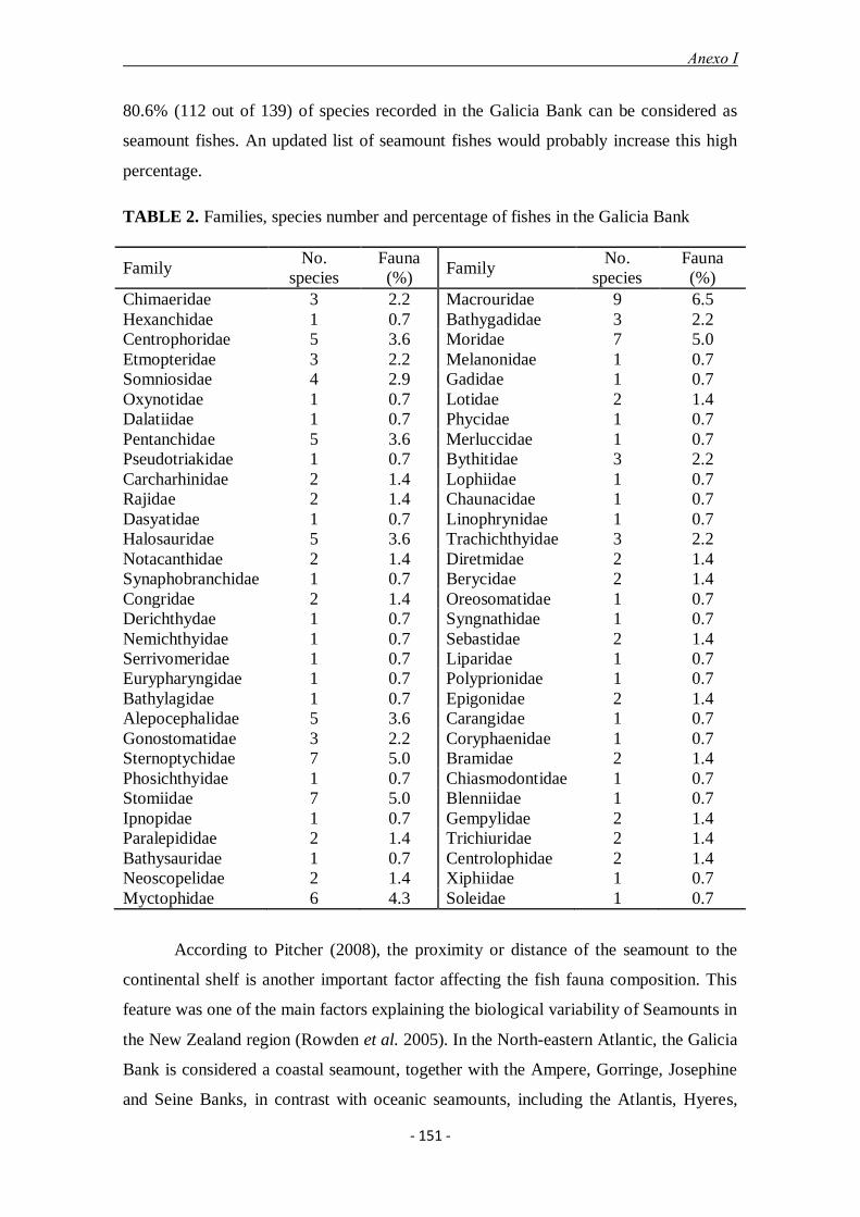
Anexo I
- 151 -
80.6% (112 out of 139) of species recorded in the Galicia Bank can be considered as
seamount fishes. An updated list of seamount fishes would probably increase this high
percentage.
TABLE 2. Families, species number and percentage of fishes in the Galicia Bank
Family No.
species
Fauna
(%) Family
No.
species
Fauna
(%)
Chimaeridae 3 2.2 Macrouridae 9 6.5
Hexanchidae 1 0.7 Bathygadidae 3 2.2
Centrophoridae 5 3.6 Moridae 7 5.0
Etmopteridae 3 2.2 Melanonidae 1 0.7
Somniosidae 4 2.9 Gadidae 1 0.7
Oxynotidae 1 0.7 Lotidae 2 1.4
Dalatiidae 1 0.7 Phycidae 1 0.7
Pentanchidae 5 3.6 Merluccidae 1 0.7
Pseudotriakidae 1 0.7 Bythitidae 3 2.2
Carcharhinidae 2 1.4 Lophiidae 1 0.7
Rajidae 2 1.4 Chaunacidae 1 0.7
Dasyatidae 1 0.7 Linophrynidae 1 0.7
Halosauridae 5 3.6 Trachichthyidae 3 2.2
Notacanthidae 2 1.4 Diretmidae 2 1.4
Synaphobranchidae 1 0.7 Berycidae 2 1.4
Congridae 2 1.4 Oreosomatidae 1 0.7
Derichthydae 1 0.7 Syngnathidae 1 0.7
Nemichthyidae 1 0.7 Sebastidae 2 1.4
Serrivomeridae 1 0.7 Liparidae 1 0.7
Eurypharyngidae 1 0.7 Polyprionidae 1 0.7
Bathylagidae 1 0.7 Epigonidae 2 1.4
Alepocephalidae 5 3.6 Carangidae 1 0.7
Gonostomatidae 3 2.2 Coryphaenidae 1 0.7
Sternoptychidae 7 5.0 Bramidae 2 1.4
Phosichthyidae 1 0.7 Chiasmodontidae 1 0.7
Stomiidae 7 5.0 Blenniidae 1 0.7
Ipnopidae 1 0.7 Gempylidae 2 1.4
Paralepididae 2 1.4 Trichiuridae 2 1.4
Bathysauridae 1 0.7 Centrolophidae 2 1.4
Neoscopelidae 2 1.4 Xiphiidae 1 0.7
Myctophidae 6 4.3 Soleidae 1 0.7
According to Pitcher (2008), the proximity or distance of the seamount to the
continental shelf is another important factor affecting the fish fauna composition. This
feature was one of the main factors explaining the biological variability of Seamounts in
the New Zealand region (Rowden et al. 2005). In the North-eastern Atlantic, the Galicia
Bank is considered a coastal seamount, together with the Ampere, Gorringe, Josephine
and Seine Banks, in contrast with oceanic seamounts, including the Atlantis, Hyeres,
Anexo I
- 152 -
Irving, Meteor and Plato Banks, located offshore (Gofas 2007; Surugiu et al. 2008).
Nevertheless, some results on inter-seamount invertebrate faunal similarity highlight the
separation of the Galicia Bank due to its isolated northern position and deep plateau
(Surugiu et al. 2008).
Of the 139 fish species reported in this paper, 99 (71.2%) have been also
reported in the continental shelf and slope of Galician waters whereas the remaining 40
species (28.8%) are exclusive of the Galicia Bank. This difference could be mainly
ascribed to a relative more intensive sampling of the Galicia Bank compared to the
deep-water areas of the Galician coast. In fact, all of the fish species captured in the
Galicia Bank have been also reported in other areas of the North-eastern Atlantic,
indicating the lack of endemic species in the Bank.
Seamounts have been frequently described as biological islands harbouring
unique or characteristic fauna with high rates of endemism. However many of these
characterizations have been questioned in the last years (McClain 2007) and the levels
of endemic species on seamounts may vary between individual seamounts, regions and
taxa, and may, in some cases, be limited to species with a low dispersal ability
(Secretariat of the Convention on Biological Diversity 2008). A recent study suggest
that seamount fish faunas are not unique to seamounts but are, in fact, similar to the
fauna inhabiting the surrounding region (Lundsten et al., 2009), which is in agreement
with our results.
Among the ecological factors pointed out by Pitcher (2008), the presence of
corals was related with the presence and abundance of seamount fishes. Corals provide
an important source of three dimensional structures in the predominantly sedimentary
habitats of deeper waters, acting as refuge habitat for many fish species (Söffker et al.
2011). Many fishes show spatial co-occurrence with deep-water corals and fish catches
have been found to be higher in and around deep-water coral reefs (Clark et al. 2006).
Studies on Lophelia coral reefs in the Northeast Atlantic have recorded the presence of
25 fish species (Costello et al. 2005). In the case of the Galicia Bank, the main areas of
cold-water coral mounds and reefs have been identified between 620 and 1,125 m depth
(Somoza et al. 2014). Although the relationships among fishes and corals in the Galicia
Bank was not analysed, most of the fish species (about 100) were captured within this
range of depth, which seems to indicate a positive relationship between corals and the
presence and abundance of fishes. Moreover, N. helgae and G. latifrons, two fish
Anexo I
- 153 -
species particularly associated with coral reef habitats off Ireland (Söffker et al. 2011),
were also present in the Bank.
Seamount communities are highly vulnerable to impacts from fisheries and
recovery from fishing impacts is a lengthy process (Schlacher et al. 2010). Thus, the
fishing activity is another feature to be considered when evaluating the conservation
status of seamounts in relation to threats (Pitcher 2008). Evidences of fishing activity in
the Galicia Bank were observed by the presence of derelict fishing gears, mainly gill
nets. The first fishing activities in the area were reported in 1971, initially with bottom
longlines and some years later with bottom gillnets (volantas) targeting L. piscatorius,
P. americanus, E. telescopus, Beryx splendens and P. blennoides. In the late 1970's and
early 1980's a fishery with pelagic longline targeting X. gladius and B. brama was
developed. During the 1990's, there was also some fishing activity targeting deep-water
sharks with bottom longline. Some attempts to fish by bottom trawling were also
recorded in the area. However, the scarcity of sedimentary areas suitable for trawling
combined with the low catch rate of commercial species and the high presence of corals
discouraged the development of this fishery.
During the last years, the fishing activity in the Galicia Bank has been greatly
reduced because of several aspects such as the great distance from homeports together
with the prohibition of fishing during weekends since 2002, the scarcity of high value
species and the zero catches for deep-water sharks set by the European Union since
2010. Nowadays, only 3 vessels are sporadically moving to the Bank targeting L.
piscatorius with gillnet. Thus, and in general terms, the fishing activity carried out in
the Bank has been low and has progressively decreased. This low level of fishing
activity, specially the absence of bottom trawl, has preserved the benthic environment of
the Galicia Bank in a relatively good state, with well-preserved deep-sea biotopes of
conservation importance such as coral communities.
Regarding the occurrence of singular fish species, the presence of B. ocellaris in
the Bank at 762-799 m depth set a new deep record for the species. B. ocellaris is a
demersal species usually distributed between 10 and 400 m depth that typically closes
its life-cycle in coastal waters without apparent dependence on seamounts. However,
this species has been recently captured in the Concepción Bank seamount, at 390 m

Anexo I
- 154 -
depth (IEO 2013). Both findings confirm the presence of B. ocellaris not only in the
continental or island shelves but also in coastal seamounts located near these areas.
TABLE 3. Species list to be threatened according to the OSPAR list of threatened
and/or declining species (www.ospar.org), IUCN red list of threatened species
(www.iucnredlist.org) and FishBase (www.fishbase.org). Abbreviations: critically
endangered (CR), vulnerable (VU), very high vulnerability (VHV), high to very high
vulnerability (HHV) and high vulnerability (HV).
Family Species OSPAR IUCN FishBase
Hexanchidae Hexanchus griseus — — VHV
Pentanchidae Galeus melastomus — — HV
Pentanchidae Apristurus aphyodes — — HHV
Pseudotriakidae Pseudotriakis microdon — — HHV
Carcharhinidae Isurus oxyrhinchus — VU VHV
Carcharhinidae Prionace glauca — — HHV
Dalatiidae Dalatias licha — EN VHV
Somniosidae Centroscymnus
coelolepis
VU EN HV
Somniosidae Centroselachus
crepidater
— — VHV
Somniosidae Somniosus rostratus — — VHV
Somniosidae Scymnodon ringens — — HV
Oxynotidae Oxynotus paradoxus — — HV
Centrophoridae Centrophorus granulosus VU CR VHV
Centrophoridae Centrophorus squamosus VU EN VHV
Centrophoridae Deania calcea — EN HHV
Centrophoridae Deania hystricosa — — HHV
Centrophoridae Deania profundorum — — HHV
Rajidae Dipturus batis VU CR VHV
Dasyatidae Pteroplatitrygon violacea — — HHV
Chimaeridae Chimaera monstrosa — — HHV
Chimaeridae Chimaera opalescens — — HV
Chimaeridae Hydrolagus affinis — — HHV
Congridae Conger conger — — VHV
Polyprionidae Polyprion americanus — — VHV
Gempylidae Ruvettus pretiosus — — VHV

Anexo I
- 155 -
Centrolophidae Centrolophus niger — — VHV
Alepocephalidae Alepocephalus bairdii — — HHV
Alepocephalidae Alepocephalus rostratus — — HHV
Macrouridae Coryphaenoides
rupestris
— EN HHV
Moridae Lepidion guentheri — — HHV
Moridae Antimora rostrata — — HHV
Ophididae Spectrunculus grandis — — HHV
Lophiidae Lophius piscatorius — — HHV
Trachichthyidae Hoplostethus atlanticus VU VU HHV
Berycidae Beryx decadactylus — — HHV
Sebastidae Trachyscorpia cristulata — — HHV
Epigonidae Epigonus telescopus — — HHV
Bramidae Brama brama — — HHV
Gempylidae Nesiarchus nasutus — — HHV
Trichiuridae Aphanopus carbo — — HHV
Xiphiidae Xiphias gladius — — HHV
Alepocephalidae Roulenia atrita — — HV
Macrouridae Coelorhynchus
coelorhynchus
— — HV
Macrouridae Coryphaenoides
mediterraneus
— — HV
Macrouridae Malacocephalus laevis — — HV
Moridae Halargyreus johnsonii — — HV
Moridae Mora moro — — HV
Phycidae Phycis blennoides — — HV
Merluccidae Merluccius merluccius — — HV
Bythitidae Cataetyx laticeps — — HV
Trachichthyidae Hoplostethus cadenati — — HV
Trachichthyidae Hoplostethus
mediterraneus
— — HV
Berycidae Beryx splendens — — HV
Oreosomatidae Neocyttus helgae — — HV
Carangidae Trachurus trachurus — — HV
Bramidae Taractes asper — — HV
Trichiuridae Benthodesmus simonyi — — HV

Anexo I
- 156 -
The presence in seamounts of unusual species, scarcely known on the
continental shelf, has been related to the hypothesis that seamounts and islands are used
as "stepping stones" for the transoceanic dispersal of species (Wilson & Kaufmann
1987). Examples of this could be the cases of N. helgae (Moore et al. 2008) or P.
dalwigki (Bañón et al. 2002), but also of several species such as P. splendens, G. granti,
A. oleosa and N. microchir, which have a northward eastern Atlantic distribution along
the Canary and Azores Islands and the Galicia Bank (Bañón et al. 2011).
During the last two decades, there has been an internationally concern in order to
protect the deep-sea ecosystems. Thus, the concept of ‗Ecologically or Biologically
Significant Marine Areas‘ (EBSAs) has been proposed to identify open ocean and deep-
sea habitats in need of protection (Clark et al. 2014). According to this, seamounts are
considered as EBSAs due to their importance as refuge locations for threatened,
endangered and declining species. Seamount fishes, particularly seamount-aggregating
fishes, have a higher intrinsic vulnerability than other groups of fishes due to a longer
lifespan, later sexual maturation, slower growth and lower natural mortality (Morato et
al. 2004).
Based on life history and ecological characteristics, several authors have placed
the seamount fishes at the extreme end of the vulnerability spectrum. Morato et al.
(2006) indicated that seamount species were more at risk than species that did not occur
on seamounts, and that aggregating species were even more vulnerable. Considering the
three databases (OSPAR, IUCN and FishBase) used to evaluate this criterion, 9 species
(6%) were considered as threatened according to IUCN, 5 species (3%) according to
OSPAR and 58 (42%) according to FishBase (Table 3). These differences are mainly
due to the different criteria used to estimate the vulnerability. OSPAR criteria are based
on the global and regional importance and on the presence of rare, sensitive, declining
and key stone species. Those of the IUCN are inferred from several parameters mainly
focusing on species population dynamics, which are not available for most of the listed
species (data deficient), whereas FishBase provides vulnerability values for fish mainly
based on fish life-history traits. Vulnerability data provided by FishBase are
uncorrelated with those provided by IUCN, but both should be used together in studies
dealing with fish conservation (Strona 2014). However, whenever data from IUCN are
not available or in general macro-ecological studies focusing on large sets of species,
the use of FishBase vulnerability data appears to be the best option (Strona et al. 2013).

Anexo I
- 157 -
Thus, 42% of the fish species recorded in the Galicia Bank should be considered as
threatened species. In addition, the high fish biodiversity composed mainly of deep-
water species, and their high vulnerability should be strong reasons to declare the
Galicia Bank as a MPA by the Spanish government.
Acknowledgements
This study was partially founded by the Spanish Environment Ministry (ECOMARG3
project) and by the EC contract INDEMARES-LIFE (07/ NAT /E/000732). We wish to
thank to all the participants in the surveys ―ECOMARG 09‖, ―INDEMARES 0810‖ and
―INDEMARES 0811‖ to the crews of the R/V Cornide de Saavedra (IEO) R/V Thalassa
(IFREMER-IEO) and the R/V Miguel Oliver (IEO). The Autonomous Government of
Galicia (Xunta de Galicia) has collaborated in this project. Special thanks to Alejandro
de Carlos (University of Vigo) for his valuable comments. The results of this paper will
fulfil the PhD requirements of Rafael Bañón Díaz in the University of Vigo.
References
Albaigés, J.B., Morales-Nin, B. & Vilas, F. (2006) The Prestige Oil Spill: A scientific
response. Marine Pollution Bulletin, 53, 205–207.
http://dx.doi.org/10.1016/j.marpolbul.2006.03.012
Alonso, B., Ercilla, G., Casas, D., Estrada, F., Farrán, M., García, M., Rey, D. & Rubio,
B. (2008) Late Pleistocene and Holocene sedimentary facies on the SW Galicia
Bank (Atlantic NW Iberian Peninsula). Marine Geology, 249, 46–63.
http://dx.doi.org/10.1016/j.margeo.2007.09.012
Arronte, J.C. & Heredia, J. (2006) First record of Diretmichthys parini (Beryciformes:
Diretmidae) in the Bay of Biscay (northeast Atlantic). Cybium, 30, 383–384.
Bouchet, P. & Metivier, B. (1988) Campagne océanographique "Seamount 1". Compte
rendu et liste des stations. MNHN, unpublished.
Bañón, R., Casas, J.M. Piñeiro C.G. & Covelo, M. (1997) Capturas de peces de
afinidades tropicales en aguas atlánticas de Galicia (NO de la península Ibérica).
Boletín del Instituto Español de Oceanografía, 13, 57–66.

Anexo I
- 158 -
Bañón, R., Del Río, J.L., Piñeiro, C. & Casas, M. (2002) Occurrence of tropical affinity
fishes In Galician waters NW Spain. Journal Marine Biology Association. U.K.,
82, 877–880.
http://dx.doi.org/10.1017/S0025315402006288
Bañón, R., Piñeiro, C. & Casas, M. (2006a) Biological aspects of deep-water sharks
Centroscymnus coelolepis and Centrophorus squamosus off Galician waters
(NW Spain). Journal Marine Biology Association U.K. 86, 847–852.
http://dx.doi.org/10.1017/S0025315406013774
Bañón, R., Pietsch, T.W. & Piñeiro, C.-G. (2006b) New record of Linophryne coronata,
(Lophiiformes, Linophrynidae) from the North-eastern Atlantic Ocean. Cybium,
30, 385–386.
Bañón, R., Piñeiro, C. & Casas, M. (2008) Biological observations on the gulper shark
Centrophours granulosus (Chondrichthyes: Centrophoridae) off the coast of
Galicia (north-west Spain, eastern Atlantic). Journal Marine Biology
Association U.K., 88, 411–414.
http://dx.doi.org/10.1017/S0025315408000787
Bañón, R., Villegas-Ríos, D., Serrano, A., Mucientes, G. & Arronte, J.C. (2010) Marine
fishes from Galicia (NW Spain): an updated checklist. Zootaxa, 2667, 1–27.
Bañón, R., Arronte, J.C., Serrano, A. & Sánchez, F. (2011) First records of
Purplemouthed conger Pseudophichthys splendens (Anguilliformes: Congridae)
from the Galicia Bank (NW Spain). A northward range extension of their
distribution in the eastern Atlantic. Cybium, 35, 262–264.
Bañón, R., Arronte, J.C., Barros-García, D., Vázquez-Dorado, S. & de Carlos, A.
(2013a) Taxonomic study of Bathygadidae fishes (Gadiformes) from Atlantic
Spanish waters combining morphological and molecular approaches. Zootaxa,
3746, 552–566.
http://dx.doi.org/10.11646/zootaxa.3746.4.3.
Bañón, R., Arronte, J.C., Vázquez-Dorado, S.,. del Río, J.L & de Carlos, A. (2013b).
DNA barcoding of the genus Lepidion (Gadiformes: Moridae) with recognition
of Lepidion eques as a junior synonym of Lepidion lepidion. Molecular Ecology
Resources, 13, 189–199.
http://dx.doi.org/10.1111/1755-0998.12045

Anexo I
- 159 -
Black, M., Hill, M.N., Laughton, A.S. & Matthews, D.H. (1964) Three non-magnetic
seamounts off the Iberian coast. Quarterly Journal of the Geological Society,
120, 477–513.
http://dx.doi.org/10.1144/gsjgs.120.1.0477
Cartes, J.E., V. Papiol, I. Frutos, E. Macpherson, C. González-Pola, A. Punzón, X.
Valeiras, A. Serrano. 2014. Distribution and biogeographic trends of decapod
assemblages from Galicia Bank (NE Atlantic) at depths between 700 and 1800
m, with connexions to regional water masses. Deep-Sea Research II, 106, 165–
178.
http://dx.doi.org/10.1016/j.dsr2.2013.09.034
Cheung, W.W.L., T.J. Pitcher and D. Pauly (2005). A fuzzy logic expert system to
estimate intrinsic extinction vulnerabilities of marine fishes to fishing.
Biological Conservation, 124, 97–111.
http://dx.doi.org/10.1016/j.biocon.2005.01.017
Clark, M.R., Tittensor, D., Rogers, A.D., Brewin, P., Schlacher, T., Rowden, A., Stocks,
K. & Consalvey, M. (2006) Seamounts, deep-sea corals and fisheries:
vulnerability of deep-sea corals to fishing on seamounts beyond areas of
national jurisdiction. UNEP-WCMC, Cambridge, 80 pp.
Clark, M.R., Watling, L., Rowden, A.A., Guinotte, J.M. & Smith, C.R. (2011) A global
seamount classification to aid the scientific design of marine protected area
networks. Ocean & Coastal Management, 54, 19–36.
http://dx.doi.org/10.1016/j.ocecoaman.2010.10.006
Clark, M.R., Rowden, A.A., Schlacher, Guinotte, J., Dunstan, P.K., Williams A.,
O‘Hara, T.D., Watling, L., Niklitschek, E. & Tsuchida, S. (2014) Identifying
Ecologically or Biologically Significant Areas (EBSA): A systematic method
and its application to seamounts in the South Pacific Ocean. Ocean & Coastal
Management, 91, 65–79.
http://dx.doi.org/10.1016/j.ocecoaman.2014.01.016
Costello, M.J., McCrea, M., Freiwald, A., Lundalv, T., Jonsson, L., Bett, B.J., Van
Weering, T.C.E., De Hass, H., Roberts, M.J. & Allen, D. (2005) Role of cold-
water Lophelia pertusa coral reefs as fish habitat in the NE Atlantic. In:

Anexo I
- 160 -
Freiwald, A. & Roberts, J.M. (Eds.), Cold-water corals and ecosystems. 2nd
International Symposium on Deep-Sea Corals. Springer, Berlin, pp. 771–805.
Cristobo, J., Ríos, P., Preciado, I., Serrano, A., González, D., Polonio, V., Fernández, J.
& Sánchez, F. (2010) Poriferos del Banco de Galicia recolectados durante la
expedición ECOMARG 09. XVI Simposio Ibérico de Estudios de Biología
Marina. Alicante (España), 6-10 Septiembre 2010.
Cristobo, J., Rios, P., Pomponi, S.A. & Xavier, J. (2015) A new carnivorous sponge,
Chondrocladia robertballardi sp. nov. (Porifera: Cladorhizidae) from two north-
east Atlantic seamounts. Journal of the Marine Biological Association of the
United Kingdom.
http://dx.doi.org/10.1017/S0025315414001325
Díaz, J., Gallart, J. & Gaspà, O. (2007) A typical seismic signals at the Galicia Margin,
North Atlantic Ocean, related to the resonance of subsurface fluid-filled cracks.
Tectonophysics, 433, 1–13.
http://dx.doi.org/10.1016/j.tecto.2007.01.004
Duineveld, G.C.A., Lavaleye, M.S.S., Berghuis, E.M. (2004) Particel flux and food
supply to a seamount cold-water coral community (Galicia Bank, NW Spain).
Marine Ecology Progress Series, 277, 13–23.
http://dx.doi.org/10.3354/meps277013
Durán, P. & Román, E. (2000) Spanish experimental fishings: a cooperative research
initiative between scientists and the local fishing industry. ICES CM 2000/W:03,
1–18.
Ellis, J.R., Engelhard, G.H. & Pinnegar, J.K. (2007) Ecotypology of fishes in the eastern
North Atlantic. RECLAIM, 26: 68 p. Available from:
http://www.climateandfish.eu (accessed 12/12/2014).
Ebert, D. A., Stehmann, M.F.W. (2013) Sharks, batoids, and chimaeras of the North
Atlantic. FAO Species Catalogue for Fishery Purposes No 7. FAO, Rome, 523
pp.
Ercilla, G., Córdoba, D., Gallart, J., Gràcia, E., Muñoz, J.A., Somoza, L., Vázquez, J.,
Vilas, F. & Prestige Group. (2006) Geological characterization of the Prestige

Anexo I
- 161 -
sinking area. Marine Pollution Bulletin, 53, 208–219.
http://dx.doi.org/10.1016/j.marpolbul.2006.03.016
Ercilla, G. & F. Vilas. (2008) Geological characterization of the Galicia Bank Region
(Atlantic Ocean, NW Iberia): The marine geology community's response to the
Prestige disaster. Marine Geology, 249: 1–6.
http://dx.doi.org/10.1016/j.margeo.2007.09.008
Eschmeyer, W.N. (Ed.) (2014) Catalog of Fishes, genera, species, references. Electronic
version. Available from:
http://research.calacademy.org/research/ichthyology/catalog/fishcatmain.asp
(accessed 1 November 2014)
Fisher, M.J. (1969) Benthonic foraminifera from the Maestrichtian chalk of Galicia
Bank, West of Spain. Palaeontology, 12, 189–200.
Flach, E., Muthumbi, A. & Heip, C. (2002) Meiofauna and macrofauna community
structure in relation to sediment composition at the Iberian margin compared to
the Goban Spur (NE Atlantic). Progress in Oceanography, 52, 433–457.
http://dx.doi.org/10.1016/S0079-6611(02)00018-6
Froese, R. & Sampang, A. (2004) Taxonomy and biology of seamount fishes. In:
Morato, T. & Pauly, D. (Eds.), Seamounts: biodiversity and fisheries. Fisheries
Centre Research Reports 12 (5), Vancouver, pp. 25–31.
Froese, R. & Pauly, D. (Eds.) (2014) FishBase. World Wide Web electronic publication.
Available from: http://www.fishbase.org (accessed 19 November 2014)
Gofas, S. (2007) Rissoidae (Mollusca: Gastropoda) from the northeast Atlantic
seamounts. Journal of Natural History, 41, 779–885.
http://dx.doi.org/10.1080/00222930701298085
Gordon, J.D.M. (2001) Open Ocean fisheries for Deep-water species. In: Steele, J.
Thorpe, S. & Turekian, K. (Eds.), Encyclopedia of Ocean Sciences, Academic
Press, pp. 2023-2030.
http://dx.doi.org/10.1006/rwos.2001.0470
Ho, H-C. & Last, P.R. (2013) Two new species of the coffinfish genus Chaunax
(Lophiiformes: Chaunacidae) from the Indian Ocean. Zootaxa, 3710, 436–448.
http://dx.doi.org/10.11646/zootaxa.3710.5.3

Anexo I
- 162 -
Howell, K.L., Mowles, S.L. & Foggo, A. (2010) Mounting evidence: near-slope
seamounts are faunally indistinct from an adjacent bank. Marine Ecology, 31,
52–62.
http://dx.doi.org/10.1111/j.1439-0485.2010.00368.x
Iglésias, S.P. Toulhoat, L. & Sellos, D.Y. (2010) Taxonomic confusion and market
mislabelling of threatened skates: important consequences for their conservation
status. Aquatic Conservation: Marine and Freshwater Ecosystems, 20, 319–333.
http://dx.doi.org/10.1002/aqc.1083
IEO (2013) Caracterización del Banco de La Concepción. Informe del Instituto Español
de Oceanografía-Centro Oceanográfico de Canarias. Proyecto LIFE+
INDEMARES (LIFE07/NAT/E/000732). Fundación Biodiversidad, Madrid, 278
pp.
IUCN (2014) The IUCN Red List of Threatened Species. Version 2014.2. Available
from: http://www.iucnredlist.org (accessed 23 November 2014).
Johnston, P.A., Santillo, D (2004) Conservation of seamount ecosystems: application of
a marine protected areas concept. Archive of Fisheries and Marine Research 51,
305–319.
Kenaley, C.P., Hartel, K.E. (2005) A revision of Atlantic species of Photostomias
(Teleostei: Stomiidae: Malacosteinae), with a description of a new species.
Ichthyological Research, 52, 251–263.
http://dx.doi.org/10.1007/s10228-005-0281-7
Luchetti, E.A., Iglésias, S.P. & Sellos, D.Y. (2011) Chimaera opalescens n. sp., a new
chimaeroid (Chondrichthyes: Holocephali) from the north-eastern Atlantic
Ocean. Journal of Fish Biology, 79, 399–417.
http://dx.doi.org/10.1111/j.1095-8649.2011.03027.x
McClain, C.R. (2007) Seamounts: identity crisis or split personality? Journal of
Biogeography, 34, 2001–2008.
http://dx.doi.org/10.1111/j.1365-2699.2007.01783.x
Morato, T., Cheung, W.W.L. & Pitcher, T.J. (2004) Taxonomy and biology of
seamount fishes In: Morato, T. & Pauly, D. (Eds.), Seamounts: biodiversity and
fisheries, 12. Fisheries Centre Research Reports, Vancouver, pp. 51–60.
Anexo I
- 163 -
Morato, T., Cheung, W.W.L. & Pitcher, T.J. (2006) Vulnerability of seamount fish to
fishing: fuzzy analysis of life history attributes. Journal of Fish Biology, 68,
209–221.
http://dx.doi.org/10.1111/j.0022-1112.2006.00894.x
Moore, J.A., Auster, P.J., Calini, D., Heinonen, K., Barber, K. & Hecker, B. (2008)
False Boarfish Neocyttus helgae in the Western North Atlantic. Bulletin of the
Peabody Museum of Natural History, 49, 31–41.
http://dx.doi.org/10.3374/0079-032X(2008)49[31:FBNHIT]2.0.CO;2
Nieto, A., Ralph, G.M., Comeros-Raynal, M.T., Kemp, J., García Criado, M., Allen,
D.J., Dulvy, N.K., Walls, R.H.L., Russell, B., Pollard, D., García, S., Craig, M.,
Collette, B.B., Pollom, R., Biscoito, M., Labbish Chao, N., Abella, A., Afonso,
P., Álvarez, H., Carpenter, K.E., Clò, S., Cook, R., Costa, M.J., Delgado, J.,
Dureuil, M., Ellis, J.R., Farrell, E.D., Fernandes, P., Florin, A-B., Fordham, S.,
Fowler, S., Gil de Sola, L., Gil Herrera, J., Goodpaster, A., Harvey, M., Heessen,
H., Herler, J., Jung, A., Karmovskaya, E., Keskin, C., Knudsen, S.W.,
Kobyliansky, S., Kovačić, M., Lawson, J.M., Lorance, P., McCully Phillips, S.,
Munroe, T., Nedreaas, K., Nielsen, J., Papaconstantinou, C., Polidoro, B.,
Pollock, C.M., Rijnsdorp, A.D., Sayer, C., Scott, J., Serena, F., Smith-Vaniz,
W.F., Soldo, A., Stump, E. and Williams, J.T. (2015) European Red List of
marine fishes. Publications Office of the European Union, Luxembourg, 81 pp.
http://dx.doi.org/10.2779/082723
OSPAR (2014) OSPAR List of Threatened and/or Declining Species and Habitats.
Available from: http://www.ospar.org/ (accessed 29 December 2014)
Piñeiro, C.G., Casas, M. & Araújo, H. (2001). Results of Exploratory deep-sea fishing
survey in the Galician Bank: biological aspects on some of seamount-associated
fish (ICES division IXb). NAFO SCR Doc. 01/146 Serial No. N4540, 1–7.
Pitcher, T.J. (2008) The sea ahead: challenges to marine biology from seafood
sustainability. Hydrobiologia, 606,161–185.
http://dx.doi.org/10.1007/s10750-008-9337-9
Quéro, J.C., Porche, P. & Vayne, J.J. (2003) Guide des poissons de l‘Atlantique
européen. Delachaux et Niestlé, Paris, 465 pp.

Anexo I
- 164 -
Rey, D., Rubio, B., Mohamed, K., Vilas, F., Alonso, B., Ercilla, G. & Rivas, T. (2008)
Detrital and early diagenetic processes in Late Pleistocene and Holocene
sediments from the SW Galicia Bank inferred from high-resolution
environmagnetic and geochemical records. Marine Geology, 249, 64–92.
http://dx.doi.org/10.1016/j.margeo.2007.09.013
Rodríguez-Cabello, C., Pérez, M. & Bañón, R. (2014) Occurrence of Apristurus species
in the Galicia Bank Seamount (NE Atlantic). Journal of Applied Ichthyology, 30,
906–915.
http://dx.doi.org/10.1111/jai.12480
Rolán, E. & Pedrosa, G.P.G. (1981) Molluscs collected at the Galizia Bank (Spain). La
Conchiglia, 13, 6-7.
Rowden, A.A, Clark, M.R. & Wright, I.C. (2005) Physical characterisation and a
biologically focused classification of ―seamounts‖ in the New Zealand region.
New Zealand Journal of Marine and Freshwater Research, 39, 1039–1059.
http://dx.doi.org/10.1080/00288330.2005.9517374
Ruiz-Villarreal, M., Gonzalez-Pola, C., Diaz del Rio, G., Lavin, A., Otero, P.,
Piedracoba, S. & Cabanas, J.M. (2006) Oceanographic conditions in North and
North West Iberia and their influence on the Prestige oil spill. Marine Pollution
Bulletin, 53, 220–238.
http://dx.doi.org/10.1016/j.marpolbul.2006.03.011
Sanjuán, A., De Carlos, A., Rodríguez-Cabello, C., Bañón, R., Sánchez, F. & Serrano,
A. (2012) Molecular identification of the Arrowhead Dogfish Deania
profundorum (Centrophoridae) from the northern waters of the Iberian
Peninsula. Marine Biology Research, 8, 901–905.
http://dx.doi.org/10.1080/17451000.2012.692160
Schlacher, T.A., Rowden, A.A., Dower, J.F. & Consalvey, M. (2010) Seamount science
scales undersea mountains: new research and outlook. Marine Ecology, 31, 1–
13.
http://dx.doi.org/10.1111/j.1439-0485.2010.00396.x
Secretariat of the Convention on Biological Diversity (2008) Synthesis and review of
the best available scientific studies on priority areas for biodiversity
conservation in marine areas beyond the limits of national jurisdiction.

Anexo I
- 165 -
Technical Series, 37. Secretariat of the Convention on Biological Diversity,
Montreal, 63 pp.
Sibuet, J.-C., De Charpal, O., Montadert, L. & Ryan, W.B.F. (1978) Mouvements
verticaux dans la region des bancs de Galice (Atlantique nord-est) d'après les
résultats du leg 47 B. Bulletin de la Société géologique de France, 20, 365–373.
http://dx.doi.org/10.2113/gssgfbull.S7-XX.4.365
Sibuet, J.-C., Srivastava, S.P., Enachescu, M. & Karner, G.D. (2007) Early Cretaceous
motion of Flemish Cap with respect to North America: implications on the
formation of Orphan Basin and SE Flemish Cap–Galicia Bank conjugate
margins. Geological Society, London, Special Publications, 282, 63–76.
http://dx.doi.org/10.1144/SP282.4
Söffker, M., Sloman, K.A. & Hall-Spencer, J.M. (2011) In situ observations of fish
associated with coral reefs off Ireland. Deep-Sea Research I, 58, 818–825.
http://dx.doi.org/10.1016/j.dsr.2011.06.002
Somoza, L., Ercilla, G., Urgorri, V., León, R., Medialdea, T., Paredes, M., Gonzalez,
F.J. & Nombela, M.A. (2014) Detection and mapping of cold-water coral
mounds and living Lophelia reefs in the Galicia Bank, Atlantic NW Iberia
margin. Marine Geology, 349, 73–90.
http://dx.doi.org/10.1016/j.margeo.2013.12.017
Staudigel, H., Koppers, A.A.P., Lavelle, J.W., Pitcher, T.J. & Shank, T.M. (2010) Box
1: Defining the word "seamount". Oceanography, 23, 20–21.
http://dx.doi.org/10.5670/oceanog.2010.85
Strona, G, Galli, P. & Fattorini, S. (2013) Fish parasites resolve the paradox of missing
coextinctions. Nature Communications 4, 1718, 1–5.
http://dx.doi.org/10.1038/ncomms2723
Strona, G. (2014) Assessing fish vulnerability: IUCN vs FishBase. Aquatic
Conservation: Marine and Freshwater Ecosystems, 24, 153–154.
http://dx.doi.org/10.1002/aqc.2439
Surugiu, V., Dauvin, J.-C., Gillet, P. & Ruellet, T. (2008) Can seamounts provide a
good habitat for polychaete annelids?, Example of the Northeastern Atlantic

Anexo I
- 166 -
Seamounts. Deep Sea Research I, 55, 1515–1531.
http://dx.doi.org/10.1016/j.dsr.2008.06.012
Vanney, J.R., Auxietre, J.L. & Dunand, J.P. (1979) Geomorphic provinces and the
evolution of the northwestern Iberian continental margin. Annales de l'Institut
Oceanographique, Paris, 55, 5–20.
Vázquez, J.T., Medialdea, T., Ercilla, G., Somoza, L., Estrada, F., Fernández-Puga,
M.C., Gallart, J., Gràcia, E., Maestro, A. & Sayago, M. (2008) Cenozoic
deformational structures on the Galicia Bank Region (NW Iberian continental
margin). Marine Geology, 249, 128–149.
http://dx.doi.org/10.1016/j.margeo.2007.09.014
White, M. & Mohn, C. (2004) Seamounts: a review of physical processes and their
influence on the seamount ecosystem. OASIS/National University of Ireland,
Galway, 38 pp.
White M, Mohn C (2004) Seamounts: a review of physical processes and their influence
on seamount ecosystems. OASIS (OceAnic seamounts) Report, University of
Hamburg
Wilson, R. & Kaufman, R. (1987) Seamount biota and geography. In: Keating B.H,
Fryer, P. Batiza, R. & Boehlert, G.W (Eds.), Seamounts, islands and attolls.
Geophysical Monograph, 43. American Geophysical Union, Washington, pp.
355–377.
Whitehead, P.J.P., Bauchot, M.-L. Hureau, J.-C. Nielsen, J. & Tortonese, E. (Eds.)
(1986) Fishes of the North-eastern Atlantic and the Mediterranean. Vols. I-III.
UNESCO, Paris,1473 pp.
Anexo II
167
Anexo II
Rodríguez-Cabello, C., Pérez, M. & Bañón, R. 2014. Occurrence of Apristurus species
in the Galicia Bank Seamount (NE Atlantic). Journal of Applied Ichthyology, 30 (5):
906-915.

Anexo II
168
SUMMARY
The aim of this study was to identify some Apristurus species combining
morphometric and genetic tools. Several specimens of the genus Apristurus were
caught on the Galicia Bank Seamount (NE Atlantic), between 1,460 and 1,809 m
depth, during a multidisciplinary survey carried out in 2011 within the framework of
the INDEMARES Project. Morphometric and genetic analyses were conducted to
aid the identification of the specimens collected. A total of 20 specimens were
identified, of which 18 corresponded to Apristurus aphyodes (Nakaya & Stehmann,
1998), one to A. profundorum (Goode & Bean, 1896) and one to A. melanoasper
Iglesias, Nakaya and Stehmann, 2004. Genetic results based on mtDNA COI
sequences (682–690 bp fragment of the COI gene) support the identification of A.
profundorum and A. melanoasper, with a bootstrap of 99% and 96% respectively.
The identification of A. aphyodes was also performed using a 499 bp fragment of
the 16S mitochondrial gene. These are the first records of Apristurus species from
Galician waters, which extend the known distribution area of these species and
provide more information about different biological and ecological aspects of this
complex taxonomic group.
INTRODUCTION
The genus Apristurus (Garman, 1913), is one of the largest genera of living
catsharks, with 37 species currently recognised as valid, and 55 nominal species
(Froese & Pauly, 2011). It previously belonged to the family Scyliorhinidae, but was
recently included in the family Pentanchidae, based on molecular and morphological
phylogenetic studies that showed that the family Scyliorhinidae was paraphyletic
(Maisey, 1984; Winchell et al., 2004; Iglesias et al., 2005). The resurrected family
Pentachidae differs from the Scyliorhinidae by the absence of supraorbital crests on
the chondocranium (Compagno, 1988; Iglesias et al., 2005).
Apristurus species inhabit the continental slopes and submarine elevations at
depths of 400–2,000 m in all marine waters, except for the Polar regions
(Compagno, 1984; Ebert & Stehmann, 2013). The Pacific Ocean accounts for the
greatest number of species (n=24), followed by the Atlantic (n=10) and the Indian
Ocean (n=4). One of these species, A. australis Sato, Nakaya & Yorozu, 2008
Anexo II
169
occurs in the Indian and Pacific coasts. Six species of Apristurus are known from
the North Atlantic i.e., A. laurussonii (Saemundsson, 1922) (= A. maderensis
Cadenat & Maul, 1966; = A. atlanticus (Koefoed, 1927), A. microps (Gilchrist,
1922), A. manis (Springer, 1979), A. aphyodes Nakaya & Stehmann, 1998 (=
A.atlanticus Compagno, 1984), A. profundorum (Goode and Bean, 1896) and A.
melanoasper Iglésias, Nakaya & Stehmann, 2004 (Iglesias et al., 2004). From
Galician waters, catsharks are represented by five species (Galeus atlanticus, G.
melastomus, G. murinus, Scyliorhinus canicula and S. stellaris), none of them from
the genus Apristurus (Bañón et al., 2010). However, only G. murinus has been
caught on the Galicia Bank Seamount, the other four species were found on the
continental shelf and slope.
The genus Apristurus is considered one of the most diverse and taxonomically
confusing genera among living sharks, in part due to the large number of poorly
known species (Nakaya et al., 2008a). Taxonomic revisions of Apristurus have been
previously carried out (Springer, 1979; Nakaya, 1991; Nakaya & Sato, 1998, 1999;
Iglesias et al., 2005). Despite all these revisions, taxonomic confusion still exists,
because many species are homogeneous in morphology and available material is
lacking for many species (Iglesias & Nakaya, 2004).
Galicia Bank (GB) is a large seamount located 120 miles offshore from the west
coast of Galicia (North Spain). The top of the Bank is at 600 m depth and reaches
4,000 m on its deepest side. It has a length of 50 km in the E–W direction and 90 km
in the N–S axis (Figure 1). This region comprises part of an Environment Ministry
(2004) proposal to make an inventory of the biodiversity in the Spanish seas through
the identification of valuable areas for the Natura 2000 Network. The last surveys
conducted in this area within this framework contributed to increase the number of
species that inhabit these waters and confirmed the high biodiversity in the Galicia
Bank. Although only scattered records have been published to date in this area
(Bañon et al., 2011; Sanjuan et al., 2012, a complete list of the fish fauna found in
the Galician Bank is now being processed.
Previous information on elasmobranch species present in the Galicia Bank is
limited. Piñeiro et al. (2001), reported 11 sharks for this area based on experimental
and commercial surveys, although they only provided the scientific name of six
species. In addition, biological and taxonomic studies of other deep-water sharks,
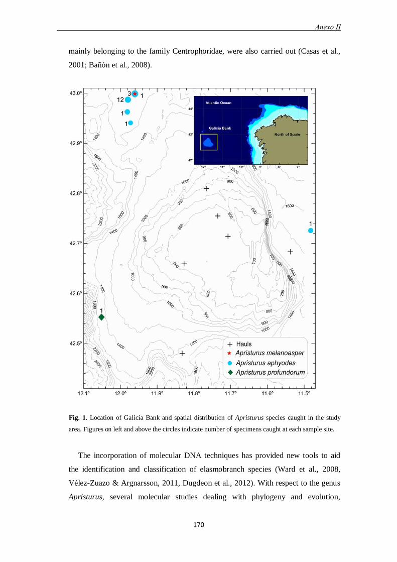
Anexo II
170
mainly belonging to the family Centrophoridae, were also carried out (Casas et al.,
2001; Bañón et al., 2008).
Fig. 1. Location of Galicia Bank and spatial distribution of Apristurus species caught in the study
area. Figures on left and above the circles indicate number of specimens caught at each sample site.
The incorporation of molecular DNA techniques has provided new tools to aid
the identification and classification of elasmobranch species (Ward et al., 2008,
Vélez-Zuazo & Argnarsson, 2011, Dugdeon et al., 2012). With respect to the genus
Apristurus, several molecular studies dealing with phylogeny and evolution,

Anexo II
171
conservation or diversity have been performed (Winchell et al., 2004; Iglesias et al.,
2005; Naylor et al., 2012). Nevertheless, genetic and morphological techniques have
their own limitations and therefore, the integration of both methodologies is
recommended (White & Last, 2012).
The aim of this study was to identify the Apristurus species caught in Galicia
Bank seamount combining morphometric and genetic tools, to increase the
knowledge of this complex taxonomic group.
MATERIAL AND METHODS
Study area
Apristurus species were caught during a multidisciplinary survey carried out in the
Galicia Bank in July 2011 within the framework of the INDEMARES project
(Figure 1). Almost all the specimens were caught using a bottom trawl net (GOG-
73) with a mesh size of 10 mm and haul duration of 30 min. Only one specimen was
caught using a beam trawl (3.5 m width, 10 mm mesh size) during a 15 min trawl
and another one with an Arcachon type suprabenthic sledge, aimed at colleting
small fauna from different water layers adjacent to the sea floor. The sea floor was
dredged for 2 min, at a speed of 2 knots (for more information about the different
gears used in these surveys visit www.ecomarg.net).
During this survey, a total of 20 hauls were performed, nine using the bottom
trawl net and eleven with the beam trawl at depths ranging from 700 to 1,809 m.
Apristurus species were recorded in five of these hauls at depths ranging from 1,459
to 1,809 m. (Table 1, Figure 1). Thirteen trawls were additionally carried out with
the suprabenthic sledge. The location and depth corresponded to the position
recorded at the end of the tow when the gear left the sea floor. Apristurus species
were identified according to several fish faunas and revisions of this genus
(Compagno, 1984; Whitehead, 1984; Iglésias et al., 2004; Iglesias, 2013; Nakaya &
Sato, 1999; Nakaya & Stehmann, 1998; Quéro et al., 2003; Springer, 1979; Ebert &
Stehmann, 2013).
Muscle samples were removed from thawed individuals and stored in 96%
ethanol. The specimens where then fixed in 10% formalin, prior to their storage in
70% ethanol. Specimens were stored in the IEO fish collection at the Oceanographic
Centre of Santander (Table 2). Photographs of the specimens and the DNA sequence

Anexo II
172
data are public available in the Barcode of Life Data Base (BOLD) with the DOI:
dx.doi.org/10.5883/DS-IEOBG10.
Tab
le 1
. D
ata
of
the
spec
imen
s ca
ugh
t an
d s
amp
led.
Gea
r G
OC
= b
ott
om
tra
wl
net
, B
T=
bea
m t
raw
l. %
O.M
.= o
rgan
ic m
atte
r per
centa
ge.
Q50 =
typ
e o
f se
dim
ent:
FS
= f
ine
sand,
VF
S =
ver
y f
ine
sand
, M
S =
med
ium
san
d.
Anexo II
173
Morphological analysis
Morphometric measurements followed Nakaya et al., (2008a). All measurements
were made point-to-point to the nearest mm. Values are expressed as a percentage of
the total length (LT). Meristic characters for teeth and dermal denticles were also
recorded and spiral valves counted for some specimens to confirm the group
identification. Dermal denticles (n=20) were randomly taken from the dorsolateral
side of the body below the first dorsal fin and mean crown length was recorded with
a binocular micrometer.
Similarity between morphometric characters was calculated using the Bray-
Curtis index (Clarke & Warwick, 2001) and the resulting dendrogram was obtained
with the group average clustering algorithm using PRIMER software. The student’s
t-test was applied to examine differences in morphometric measurements between
sexes in A. aphyodes specimens.
Genetic analysis. DNA isolation, amplification and sequencing
Total genomic DNA was extracted from ethanol-preserved muscle tissue using the
FENOSALT method (Pérez & Presa, 2011). Cytochrome oxidase I (COI) is a
reliable species tag and DNA barcoding can deliver species-level identifications
(Ward et al., 2009). A total of sixteen COI DNA sequences were obtained from
three different species of Apristurus caught in the Galicia Bank: A. aphyodes (14
sequences), A. melanoasper (1 sequence) and A. profundorum (1 sequence). A 682–
690 bp fragment of the COI gene was amplified and sequenced using the primer pair
FishF2 and FishR2 (Ward et al., 2005). Amplifications were carried out in a
Mastercycler thermocycler gradient (Eppendorf). The PCR program consisted of 5
min at 95ºC, the.n 35 cycles of 95ºC for 30 s, 50ºC for 1 min, 72ºC for 1 min and a
final extension of 10 min at 72ºC. The PCR amplification mixture of 25 µL
contained between 10 and 20 ng purified DNA, 10 pmol each primer, 0.2 mM of
dNTPs, 1.5 mM MgCl2, 1 U BioTaq DNA Polymerase (Bioline), and 2.5 µL of 10×
reaction buffer. The data set was completed with available Apristurus COI
sequences totalizing a complete data set of 71 sequences from twelve species.
In the case of A. aphyodes, COI failed to identify the sample species because
there were not available public COI sequences to conduct a barcoding comparative
identification. In this case, only 16S rRNA gene sequences were available (Iglesias
et al., 2004). Therefore, 16S rRNA gene was sequenced in four specimens

Anexo II
174
(BG11G2ASP1, BG11G10AAP1, BG11G9AAP2, BG11G2ASP3) and the data set
was completed with twelve sequences available in Genbank (AY462154-
AY462157, AY462162- AY462166 and AF358916) (Fig.2). A 427 bp fragment of
the 16S mitochondrial gene was also amplified by polymerase chain reaction (PCR)
using two primers: 16S-RA (5´-CGCCTGTTTATCAAAAACAT-3´) and 16S-RB
(5´-CCGGTCTGAACTCAGATCACGT-3´) (Palumbi et al. 1991). The PCR
program consisted of 10 min at 95ºC, then 35 cycles of 95ºC for 1 min, 55ºC for 45
s, 72ºC for 1 min and a final extension of 10 min at 72ºC. Each PCR reaction had a
total volume of 20 µL, containing between 10 and 20 ng of purified DNA, 2.5 µL of
10× NH4 Reaction Buffer (160 mM (NH4)2SO4, 670 mM Tris–HCl, pH 8.8), 1.5
µL of 8 mM pre-mixed dNTPs, 1.5 mM of MgCl2, 15 pmol of each primer, and 1 U
of BioTaq DNA polymerase (Bioline).
PCR products were cleaned before the sequencing reaction using Exo-Sap (USB)
according to the manufacturer’s protocol. The purified fragments were directly
sequenced on both DNA strands with the same primer pair used for PCR
amplification. Sequencing was performed in an ABI Prism 3100 capilar sequencer
using the BigDye Terminator Cycle Sequencing Standard (Applied Biosystems).
The final haplotypes were derived from the alignment of the forward and reverse
sequences obtained from each individual, using CHROMAS software
(http://www.technelysium.com.au/chromas.html). All Apristurus spp. public
sequences available in the BOLD database as well as 13 sequences obtained in the
present study were aligned and edited using the software Bioedit version 7.0.9.0
(Hall, 1999). The analysis involved 68 nucleotide sequences with a total of 468
positions in the final dataset. Evolutionary analyses were conducted using MEGA5
(Tamura et al., 2011). The bootstrap consensus tree based on COI sequences was
inferred from 1,000 replicates (Felsenstein, 1985) using the Neighbour-Joining
method (Saitou & Nei, 1987). The evolutionary distances were computed using the
Maximum Composite Likelihood method (Tamura & Kumar, 2004). Branches
corresponding to partitions reproduced in less than 50% bootstrap replicates were
collapsed. The percentage of replicate trees in which the associated taxa clustered
together in the bootstrap test (1,000 replicates) is shown next to the branches
(Felsenstein, 1985). All positions containing gaps and missing data were eliminated.
The molecular identification of the Apristurus species was made using i) the
identification engine provided in the Barcode of Life Data Systems (BOLD) based

Anexo II
175
on the COI sequences and, ii) a phylogenetic tree was inferred to assign unknown
sequences to species using the FINS method as described in Pérez & Presa, (2008)
and iii) the 16S sequences obtained from specimens; BG11G2ASP1,
BG11G10AAP1, BG11G9AAP2, BG11G2ASP3 were compared to those found in
GenBank using the Basic Local Alignment Search Tool algorithm (BLAST, Zhang
et al., 2000). Sequences are available online under the Genbank accession numbers
(Table 2).
Table 2. Apristurus species used in the present study with their respective codes: Sample
identification, Genbank accession numbers, Voucher collection
Species Survey_Haul Sex Length
(mm)
Sample
Identification
GenBank Accession numbers Collection Voucher
IEO COI 16 S
Apristurus
aphyodes BG1_G2 Male 259 BG11G2ASP1 KJ202061 KJ170696 IEOST2011_1_426_A
Apristurus
aphyodes BG1_G2 Female 260 BG11G2ASP3 KJ202062 KJ170698 IEOST2011_1_426_B
Apristurus
aphyodes BG1_G2 Female 247 BG11G2ASP4 KJ202063
Apristurus
aphyodes BG1_G5 Female 157 BG11G5ASP1 KJ202064
Apristurus
aphyodes BG1_G9 Male 397 BG11G9AAP1 KJ202065 IEOST2011_1_426_C
Apristurus
aphyodes BG1_G9 Female 282 BG11G9AAP2 KJ202066 KJ170697 IEOST2011_1_426_D
Apristurus
aphyodes BG1_G9 Female 260 BG11G9AAP3 KJ202067 IEOST2011_1_426_E
Apristurus
aphyodes BG1_G9 Female 261 BG11G9AAP4 KJ202068 IEOST2011_1_426_F
Apristurus
aphyodes BG1_G9 Male 249 BG11G9AAP5 KJ202069 IEOST2011_1_426_G
Apristurus
aphyodes BG1_G9 Female 242 BG11G9AAP6 KJ202070 IEOST2011_1_426_H
Apristurus
aphyodes BG1_G9 Male 252 BG11G9RF1 KJ202071
Apristurus
aphyodes BG1_G9 Male 294 BG11G9RF2 KJ202072
Apristurus
aphyodes BG1_G10 Female 377
BG11G10AAP
1 KJ202073 KJ170695 IEOST2011_1_426_K
Apristurus
aphyodes BG1_T5 Female 140 BG11T5ASP1 KJ202074
Apristurus
profundorum BG1_V7 Female 146 BG11V7ASP1 KJ202075 IEOST2011_1_437_A
Apristurus
melanoasper BG1_G2 Female 250 BG11G2ASP2 KJ202076 IEOST2011_1_436_A
RESULTS
Apristurus aphyodes Nakaya and Stehman, 1998.
Material examined. Apristurus aphyodes (see Table 2).
A total of 18 specimens were collected: six males ranging from 24.4–39.7 cm and
12 females from 22.7–37.7 cm TL at a depth range of 1,460–1,809 m (Table 1). The

Anexo II
176
majority of specimens were caught in the bottom grounds of fine sand and low
organic matter content, however, two specimens were also caught in medium and
very fine sand sediment. The bottom temperature ranged from 5.65–7.46ºC and
salinity between 35.27–35.57‰.
Description. Upper labial furrow shorter than lower one, large eyes with horizontal
diameter 1.9 to 2.5 times inter-orbital width, sub-equal size of dorsal fins, anterior
position of first dorsal fin with origin above frontal half of pelvic base, widely
spaced pectoral and pelvic fins with distance between their origins equaling head
length, 9 to 11 spiral valves in the intestine and uniform whitish coloration.
Morphometric mean values were compared between males and females (Table
1_Supp.) and significant differences were found in several characters: eye length,
head length, prebranchial length, preoral length, size of nostrils, pectoral and pelvic
lengths and distance to first dorsal fin. However, in both cases, all the specimens
sampled were juveniles. A comparison of the main morphometric measurements of
the specimens described in this study to the paratypes is shown in Table 2_Supp.
Habitat and distribution. This species is widely distributed in the eastern North
Atlantic, from Iceland to the northern Bay of Biscay (Nakaya & Stehmann, 1998),
thus, these records extend its distribution further towards the south 42º N.
Genetic results. Sixteen COI sequences (GenBank accession numbers KJ202061-
KJ202076) and four 16S sequences were obtained (GenBank accession numbers
KJ170695-KJ170698). The inferred phylogenetic tree based on obtained COI
sequences (Figure 2) clustered the 14 sequences together in the same group with a
bootstrap support of 99% (Fig. 3). The COI sequence of this species was not
available in the Genbank and BOLD databases, thus comparative identification was
not possible. However, the analysis of 16S gene sequences, carried out on four
specimens (BG11G2ASP1, BG11G10AAP1, BG11G9AAP2, BG11G2ASP3) and
subsequently compared with the sequences available in BLAST submitted by
Iglésias et al., (2004), allowed us to confirm that these samples corresponded to A.
aphyodes. The phylogenetic tree using the 16S sequences of A. aphyodes is shown
(Figure 3). All sequences were grouped with AF358916 sequence corresponding to
A. aphyodes, with a bootstrap support of 100%.

Anexo II
177
Apristurus profundorum (Goode & Bean, 1896).
Material examined. Apristurus profundorum (05/08/2011, 42.3315'N–12.0302'W,
1,460 m, 146 mm ♀ BG11V7ASP1). Only a female of 14.6 cm TL and 14.0 g
weight was caught at 1,459 m depth on medium sand sediment with a bottom
temperature and salinity of 7.45ºC and 35.57‰, respectively (Table 1).
Morphometric measurements are given in Table 1_Supp.
Description. Upper labial furrows sub-equal or shorter than lower, snout
moderately long and broad, preoral snout about 9% of total length. Eyes rather
small, diameter about 3% of total length and 2.9 to 4.0 times in interorbital width.
Mouth moderately long, large, and broadly arched; mouth and labial furrows
extending well in front of eyes (Figure 4a). Caudal fin fairly broad, with a well-
developed crest of enlarged denticles on dorsal caudal fin margin, with crest
denticles directed obliquely downwards (Figure 4b). Lateral trunk denticles of body
with crowns partly erect, giving skin surface (Figure 4c). Pectoral fins rather small,
anterior margins about 11% of total length; inner margins fairly long, about half
length of pectoral fin bases. Interspace between pectoral and pelvic fin bases
moderately long, slightly less than prespiracular length and about 15% of total
length. Pelvic fins high and broadly rounded. Interdorsal space slightly greater than
first dorsal fin base. First dorsal fin about as large as second, bases about equally
long. Spiral valve counts 10. Origin of first dorsal fin slightly behind pelvic fin mid
bases (Figure 4d).
A comparison of some morphometric measurements of this specimen and the
holotype according to Murray & Hjort (1932) is shown in Table 3_Supp.
Habitat and distribution. This species have been reported in the western North
Atlantic (Kiraly et al., 2003; Moore et al., 2003), the mid-Atlantic Ridge (Gushchin
& Kukuev, 1981) and eastern North Atlantic (Mauritania) (Compagno, 1984; Ebert
& Stehmann, 2013). This is the first record from Galician waters, which extends the
distribution of this species to the north in the Northeast Atlantic.
Genetic results. The COI sequence obtained from specimen BG11V7ASP1
(GenBank Accession No KJ202075) clustered together with the available sequences
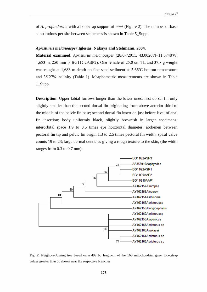
Anexo II
178
of A. profundorum with a bootstrap support of 99% (Figure 2). The number of base
substitutions per site between sequences is shown in Table 5_Supp.
Apristurus melanoasper Iglesias, Nakaya and Stehmann, 2004.
Material examined. Apristurus melanoasper (28/07/2011, 43.0026'N–11.5748'W,
1,683 m, 250 mm ♀ BG11G2ASP2). One female of 25.0 cm TL and 37.8 g weight
was caught at 1,683 m depth on fine sand sediment at 5.66ºC bottom temperature
and 35.27‰ salinity (Table 1). Morphometric measurements are shown in Table
1_Supp.
Description. Upper labial furrows longer than the lower ones; first dorsal fin only
slightly smaller than the second dorsal fin originating from above anterior third to
the middle of the pelvic fin base; second dorsal fin insertion just before level of anal
fin insertion; body uniformly black, slightly brownish in larger specimens;
interorbital space 1.9 to 3.5 times eye horizontal diameter; abdomen between
pectoral fin tip and pelvic fin origin 1.3 to 2.5 times pectoral fin width; spiral valve
counts 19 to 23; large dermal denticles giving a rough texture to the skin, (the width
ranges from 0.3 to 0.7 mm).
Fig. 2. Neighbor-Joining tree based on a 499 bp fragment of the 16S mitochondrial gene. Bootstrap
values greater than 50 shown near the respective branches

Anexo II
179
Fig. 3. Neighbor-Joining tree based on COI using Maximum Composite Likelihood distances.
Bootstrap values greater than 50 shown near the respective branches.

Anexo II
180
Fig. 4. Morphological characters of Apristurus profundorum. (a) Labial furrows, mouth shape and
nostrils; (b) Dermal denticles on dorsal caudal fin; (c) Dermal denticles on lateral dorsal body; and
(d) Dorsal and ventral fins.
A comparison of the main morphometric measurements followed Iglesias et al.,
(2004) based on all their specimens (n=53) and the one described in this study is
shown in Table 4_Supp.
Habitat and distribution. This species is widely distributed but very patchy in the
North Atlantic: northeastern U.S.A, France, Ireland and British Isles (Hartel et al.
2008; Iglesias et al., 2004; Moore et al., 2003). It also occurs in the Southeastern
Atlantic (Namibia), in the Central Indian Ocean and south of Madagascar and in the
western South Pacific (Australia, New Zealand and New Caledonia). This record
extends the known distribution of this species in the Northeast Atlantic.
Genetic results. One COI sequence was obtained (GenBank Accession KJ202076)
which is clustered within the A. melanoasper group with a bootstrap support of 95%
(Figure 2). The number of base substitutions per site between sequences is shown in
Table 5_Supp. The analysis involved 13 nucleotide sequences and was conducted
using the Maximum Composite Likelihood model (Tamura & Kumar, 2004). There
were a total of 592 positions in the final dataset because all positions containing
gaps were eliminated. All the distance values between BG11V7ASP1 and

Anexo II
181
BG11G2ASP2 with the rest of sequences are compatible with the distances between
species.
DISCUSSION
Apristurus aphyodes Nakaya & Stehman, 1998.
The comparison of the main morphometric measurements between the paratype
specimens described in the original paper of Nakaya & Stehmann (1998) and those
caught in the Galicia Bank (Table 2_Supp.) indicated that nearly all the
measurements were within the reported range with the exception of four. The upper
labial furrow, according to Nakaya & Stehmann (1998) was 2.6–3.8 (%TL) versus
4.2–4.4 in this study. The first and second dorsal fin base lengths were smaller in the
specimens described in GB (6.0–7.6 and 6.1–7.5 respectively, versus 5.6–5.9 and
5.8–6.1) as well as the caudal peduncle height (4.0–4.8 versus 3.6–3.7). The
maximum length recorded for this species is 55 cm in Rockall Trough (Moore et al.,
2013). The largest specimens caught in GB measured 39.7 and 37.7 cm, a male and
female respectively. Therefore, according to Nakaya & Stehmann (1998), who
reported that this species attained full maturity at 47 cm length and Moore et al.,
(2013) reporting L50=51.6 cm and L50=49.5 cm for male and female respectively,
all the individuals caught in this study area were juveniles.
Regarding other characters described for this species, the A. aphyodes examined in
this study confirmed: the presence of dermal denticles tricuspid; denticles on dorsal
margin of caudal fin closely packed but no enlargement in size and not forming a
crest and teeth small in upper and lower jaws with frequently five cuspids (three
cuspid in adults and two or three more lateral cuspids in small specimens). Table 6
summarizes the differences found among all the specimens examined, which could
be attributed to size or individual variation.
The identification made using 16S sequences allowed us to confirm that 11 samples
corresponded to A. aphyodes. The genetic distances (Table 5_Supp.) also indicate
the homogeneity among them with values near zero.
Apristurus profundorum (Goode & Bean, 1896)
The specimen collected in the Galicia Bank matched the general description of this
species; however, slight differences in some of the proportions of the main

Anexo II
182
characters described have been found (Table 3_Supp.), which might be due in part
to the small size of the specimen caught.
The maximum length reported for this species is 74.5 cm (Kiraly et al., 2003).
According to these authors, the holotype was collected in Hudson Canyon instead of
Delaware Bay (North West Atlantic). Further records have been reported in nearby
waters (Moore et al., 2003; Hartel et al., 2008) and in the Mid-Atlantic Ridge
(Gushchin & Kukuev, 1981). The only known records that exist in the Northeastern
Atlantic (Mauritania) need to be confirmed (Huveneers & Duffy, 2004). Thus, this
record extends the distribution of this species to the East Atlantic.
The BG11V7ASP1 COI sequence perfectly matches the A. profundorum available
sequences. All methods used to confirm this authentication, support this species
identification.
Apristurus melanoasper Iglesias, Nakaya and Stehmann, 2004
The specimen caught in GB matched all the characters previously described.
However, the dermal denticles that characterize this species and give its common
English name did not appear large at all (0.32 ± 0.03 mm), compared to the dermal
denticles of A. aphyodes of a similar size (0.36 ± 0.03 mm). This suggests that this
character might not be as evident in small specimens. A comparison of the main
morphometric measurements of this individual with those described by Iglesias et
al., (2004) is shown in Table 4_Supp.
This species was first described in 2004 in Northeast Atlantic waters (Lorien Bank)
at 1,243–1,260 m depth (Iglesias et al., 2004). However, some specimens from
Northwest Atlantic waters (North America) were also identified as A. melanoasper.
According to these authors, no significant differences were observed for
proportional measurements between European specimens and American ones. The
most significant difference found was in the size of the dermal denticles (0.3–0.7
mm), which were larger in European specimens. In 2008, this species was also
encountered in the South Pacific, Indian and South Atlantic Oceans at depths of
880–1,275 m (Nakaya et al., 2008b). The diagnosis was similar and the dermal
denticles were within the range of North Atlantic populations (0.3–0.7 mm) but
were more similar in size to American specimens. In a recently study, Naylor et al.,
(2012) questioned the classification of some specimens examined from Australia

Anexo II
183
and New Zealand based on a genetic approach and provisionally gave them the
designation Apristurus cf. melanoasper.
The genetic results based on COI allowed including this specimen (BG11G2ASP2)
with a bootstrap support of 95% within the A. melanoasper group. The sequences
accessible in the BOLD database corresponded to specimens caught in Australia,
and this might be the reason why all the sequences available for this species
clustered together with a 95% of bootstrap support and our sequence was not among
them. More sequences similar to that obtained for BG11G2ASP2 specimen could
clarify this situation. The BLAST comparison showed a maximum identity value of
99% with A. melanoasper.
References
Bañón, R.; Piñeiro, C; Casas M., 2008: Biological observations on the gulper shark
Centrophorus granulosus (Chondrichthyes: Centrophoridae) off the coast of
Galicia (north-west Spain, eastern Atlantic). J. Mar. Biol. Ass. U.K. 88(2),
411-414.
Bañón R.; Villegas-Ríos, D.; Serrano, A.; Mucientes, G.; Arronte, J.C., 2010:
Marine fishes from Galicia (NW Spain): an updated checklist. Zootaxa 2667,
1-27.
Bañón, R.; Arronte, J.C.; Serrano, A.; Sánchez, F., 2011: First records of
Purplemouthed conger Pseudophichthys splendens (Anguilliformes:
Congridae) from the Galicia Bank (NW Spain). A northward range extension
of their distribution in the eastern Atlantic. Cybium 35(3), 262-264.
Casas, J.M.; Piñeiro, C.; Bañón, R., 2001: Maturity and other biological aspects of
main deep-water squaloid sharks, in the north and northwest of the Iberian
Peninsula (ICES Divisions VIIIc, IXa and IXb). NAFO SCR Doc. 01/121:1-
10.
Clarke, K.R.; Warwick, R.M., 2001: Change in marine communities: an approach to
statistical analyses and interpretation 2nd edn. PRIMER-E, Plymouth.
Compagno, L.J.V., 1984: FAO Species Catalogue. Vol. 4: Sharks of the World. An
annotated and illustrated catalogue of shark species known to date. FAO
Fish. Synop., (125) 4(1): i-viii + 1-250; 4(2): i-x + 251-655.
Compagno, L.J.V., 1988: Sharks of the order Carcharhiniformes. Princeton
University Press, xii + 572+ pp., 157 figs., 35 plates.
Anexo II
184
Dudgeon, C.L.; Blower, D.C.; Broderick, D.; Giles, J.L.; Holmes, B.J.; Kashiwagi,
T.; Kruck, N.C.; Morgan, J.A.T.; Tillett, B.J.; Ovenden, J.R., 2012: A review
of the application of molecular genetics for fisheries management and
conservation of sharks and rays. J. Fish Biol. 80, 1789–1843.
Ebert, D.A.; Stehmann, M.F.W., 2013: Sharks, batoids, and chimaeras of the North
Atlantic FAO Species Catalogue for Fishery Purposes. Nº 7. Rome, FAO.
523 pp.
Felsenstein, J., 1985: Confidence limits on phylogenies: An approach using the
bootstrap. Evolution 39, 783-791.
Froese, R.; Pauly, D. Editors. 2011: FishBase. World Wide Web electronic
publication.www.fishbase.org, version (02/2013).
Garman, S., 1913: The Plagiostomia. Mem. Mus. Comp. Zool. Harvard, 36,1-515.
Gilchrist, J.D.F., 1922: Deep-sea fishes procured by the S.S. Pickle (Part 1) Special
Report No. III. Report of the Fisheries and Marine Biological Survey, Union
of South Africa 2, 41-79.
Goode, G.B.; Bean, T.H., 1896: Oceanic Ichthyology. US Nat. Mus. Spec. Bull. 2,
1-553.
Gushchin, A. V.; Kukuev, E. I., 1981: Notes on a collection of the ichthyofauna
from the northern part of the Mid-Atlantic Ridge. In: Fishes of the open
ocean. Eds: N. V. Parin and P. P. Shirshov, Institute of Oceanology, Moscow
(in Russian; English summary), pp. 36–40.
Hall, T.A., 1999: BioEdit: a user-friendly biological sequence alignment editor and
analysis program for Windows 95/98/NT. Nucl. Acid. S. 41, 95-98.
Hartel, K.E.; Kenaley, C.P.; Galbraith, J.K.; Sutton, T.T., 2008: Additional records
of deep-sea fishes from off greater New England. Northeastern Naturalist
15(3),317-334.
Huveneers, C.; Duffy, C., 2004: Apristurus profundorum. In: IUCN 2013. IUCN
Red List of Threatened Species. Version 2013.1. www.iucnredlist.org.
Iglesias, S.P., 2013: Chondrichthyans from the North-eastern Atlantic and the
Mediterranean (A natural classification based on collection specimens).
Provisional version 07, 01.04.2013. 106 pp. http://www.mnhn.fr/iccanam
Iglésias, S.P.; Nakaya, K., 2004: Apristurus atlanticus (Koefoed, 1927). A junior
synonym of the deepsea catshark A. laurussonii (Saemundsson, 1922)
(Chondrichthyes: Carcharhiniformes: Scyliorhinidae). Cybium 28,217–223.

Anexo II
185
Iglésias, S.P.; Nakaya, K.; Stehmann, M., 2004: Apristurus melanoasper, a new
species of deep-water catshark from the North Atlantic (Chondrichthyes:
Carcharhiniformes: Scyliorhinidae). Cybium 28,345–356.
Iglésias, S.P.; Lecointre, G.; Sellos, D.Y., 2005: Extensive paraphylies within sharks
of the order Carcharhiniformes inferred from nuclear and mitochondrial
genes. Mol. Phylogenet. Evol. 34,569–583.
Kiraly, S.J.; Moore, J.A.; Jasinski, P.H., 2003: Deepwater and other sharks of the
U.S. Atlantic Ocean Exclusive Economic Zone. Mar. Fish. Rev. 65(4),1-64.
Koefoed, E., 1927: Fishes from the sea-bottom. Rep. Sci. Res. “Michael Sars” N.
Atlantic deep-sea exped. 1910, Bergen Mus. Norway, 4(1),1-147.
Maisey, J.G., 1984: Higher elasmobranch phylogeny and biostratigraphy. Zool. J.
Linn. Soc. 82,33–54.
Moore, J.A.; Hartel, K.E.; Craddock, J.E.; Galbraith, J.K., 2003: An annotated list of
deepwater fishes from off the New England region, with new area records.
Northeast. Nat. 10(2),159-248.
Moore, D.M.; Neat, F.C.; Mccarthy, I.D., 2013: Population biology and ageing of
the deep water sharks Galeus melastomus, Centroselachus crepidater and
Apristurus aphyodes from the Rockall Trough, north-east Atlantic. J. Mar.
Biol. Ass. U.K. page 1 of 10.
Murray, J.; Hjort, J., 1932: Report of the scientific results of the “Michael Sars”
North Atlantic deep-sea expedition 1910. Published by the Bergen Museum.
Vol.IV. Part I.
Nakaya, K., 1991: A review of the long-snouted species of Apristurus
(Chondrichthyes, Scyliorhinidae). Copeia 1991,992-1002.
Nakaya, K.; Sato, K., 1998: Taxonomic review of Apristurus laurussonii
(Saemundsson, 1922) from the eastern North Atlantic (Elasmobranchii:
Scyliorhinidae). Cybium 22,149–157.
Nakaya, K.; Sato, K., 1999: Species grouping within the genus Apristurus
(Elasmobranchii, Scyliorhinidae), pp. 307–320. In: B. Séret & J.-Y. Sire
(eds) Proceedings of the Indo-Pacific Fish Conference, 1997, Nouméa.
Société Française d’Ichtyologie & Institut de Recherche pour le
Développement, Paris.

Anexo II
186
Nakaya, K.; Stehmann, M., 1998: A new species of deep-water catshark, Apristurus
aphyodes n. sp., from the Eastern North Atlantic (Chondrichthyes:
Carcharhiniformes: Scyliorhinidae). Arch. Fish. and Mar. Res. 46(1),77-90.
Nakaya, K.; Sato, K.; Iglesias, S.P.; White, W.T., 2008a: Methodology for the
taxonomic description of members of the genus Apristurus
(Chondrichthyes:Carcharhiniformes: Scyliorhinidae). In: Descriptions of
New Australian Chondrichthyans. Eds: P.R. Last; W.T. White; J.J.
Pogonoski. CSIRO Marine & Atmospheric Research Paper 022, 358 pp.
Nakaya, K.; Sato, K.; Iglésias, S.P., 2008b: Occurrence of Apristurus melanoasper
from the South Pacific, Indian and South Atlantic Oceans
(Carcharhiniformes: Scyliorhinidae), pp. 61–74. In: Descriptions of New
Australian Chondrichthyans. Eds: P.R. Last; W.T. White; J.J. Pogonoski.
CSIRO Marine & Atmospheric Research Paper 022, 358 pp.
Naylor, G.J.P.; Caira, J.N.; Jensen, K.; Rosana, K.A.M.; White, W.T.; Last, P.R.,
2012: A DNA sequence based approach to the identification of shark and ray
species and its implications for global elasmobranch diversity and
parasitology. B. Am. Mus. Nat. Hist. 367: 262 pp.
Palumbi, S.R.; Martin, A.P.; Romano, S.L.; McMillan, W.O.; Stice, L.; Grabowski,
G., 1991: The simple fool’s guide to PCR. Dept. of Zoology, University of
Hawaii, Honolulu.
Pérez, M.; Presa, P., 2008: Validation of tRNA-Glu-cytochrome b key for the
molecular identification of twelve hake species (Merluccius spp.) and
Atlantic cod (Gadus morhua) using PCR-RFLPs, FINS and BLAST. J.Agr.
Food Chem. 56(22),10865-10871.
Pérez, M.; Presa, P., 2011: FENOSALT: Un método sintético para la extracción de
ADN de peces y moluscos. In: Métodos y Técnicas de Investigación Marina.
Ed: Estévez J.M. et al, Madrid: Technos. pp. 81-89.
Piñeiro C.G.; Casas M.; Araújo, H., 2001: Results of exploratory deep-sea fishing
survey in the Galician Bank: biological aspects on some of seamount-
associated fish (ICES Division IXb). NAFO SCR Doc. 01/146 Serial No.
N4540, 7 p.
Quéro J.C.; Porché P.; Vayne J.J., 2003: Guide des Poissons de l'Atlantique
Européen. Delachaux et Niestle (eds). Paris. pp 465.

Anexo II
187
Saemundsson, B., 1922: Zoologiske Meddelelser fra Island. 14. 11 Fiske, ny for
Island, og supplerende Oplysninger omandre, tidligere kendte. Videnskab.
Meddel. Dansk. naturhist. Foren. Kobenhaven, 74,159-201.
Sanjuán, A.; De Carlos, A.; Rodríguez-Cabello, C.; Bañón, R.; Sánchez, F.; Serrano,
A., 2012: Molecular identification of the Arrowhead Dogfish Deania
profundorum (Centrophoridae) from the northern waters of the Iberian
Peninsula. Mar. Biol. Res. 8, 901-905.
Saitou, N.; Nei, M., 1987: The neighbor-joining method: A new method for
reconstructing phylogenetic trees. Mol. Biol. Evol., 4,406-425.
Springer, S., 1979: A revision of the catsharks, family Scyliorhinidae. NOAA
Technical Report, National Marine Fisheries Service, Circular, 422,1–152.
Tamura, K.; Nei, M.; Kumar, S., 2004: Prospects for inferring very large
phylogenies by using the neighbor-joining method. Proc. Natl. Acad. Sci.
U.S.A. 101,11030-11035.
Tamura, K.; Peterson, D.; Peterson, N.; Stecher, G.; Nei, M.; Kumar, S., 2011:
MEGA5: Molecular evolutionary genetics analysis using maximum
likelihood, evolutionary distance, and maximum parsimony methods. Mol.
Biol. Evol. 28(10), 2731-2739.
Vélez-Zuazo, X.; Agnarsson, I., 2011: Shark tales: A molecular species-level
phylogeny of sharks (Selachimorpha, Chondrichthyes). Mol. Phylogenet.
Evol. 58, 207–217.
Ward, R.D.; Zemlak, T.S.; Innes, B.H.; Last, P.R.; Hebert, P.D.N., 2005: DNA
barcoding Australia’s fish species. Philos. T. R. Soc. B. 360,1847-1857.
Ward, R.D.; Holmes, B.H.; William, A.; White, T.; Last, P.R., 2008: DNA
barcoding Australasian chondrichthyans: results and potential uses in
conservation. Mar. Freshwater Res. 59, 57–71.
Ward, R.D.; Hanner, R.; Hebert, P.D.N., 2009: The campaign to DNA barcode all
fishes FISH-BOLD. J. Fish Biol. 74(2), 329–356.
White, W.T.; Last, P.R., 2012: A review of the taxonomy of chondrichthyan fishes:
a modern perspective. J. Fish Biol. 80, 901–917.
Whitehead, P.J.P., 1984: Fishes of the North-eastern Atlantic and the Mediterranean
Vol. 1. Eds: Whitehead P.J.P.; Bauchot M.L.; Hureau J.C.; Nielsen J.;
Tortonese E. UNESCO. Paris. pp. 1473.

Anexo II
188
Winchell, C.J.; Martin, A.P.; Mallatt, J., 2004: Phylogeny of elasmobranchs based
on LSU and SSU ribosomal RNA genes. Mol. Phylogenet. Evol. 31,214-224.
Zhang, Z.; Schwartz, S.; Wagner, L.; Miller, W., 2000: A greedy algorithm for
aligning DNA sequences. J. Comput. Biol. 7(1-2), 203–214.

Anexo II
- 189 -
SUPLEMENTARY TABLES
Table 1 Supplement. Morphometric characters of Apristurus species (% TL) caught in the Galicia Bank.
A. aphyodes values grouped by sex and respective mean and standard deviation (± SD) included. Values
of t-test included; characters significantly different (p<0.05) are marked (*).
Morphometriccharacter
A. prof. A.melan. A. aphyodes
Significantly different
Female Female Male (n=6) Female (n=8)
t-value p p<0.05
1. Total length (cm) 14.6 25.0 28.3 ± 5.9 27.0 ± 4.6
2. PreD2-insertion 63.0 69.2 67.3 ± 1.4 67.4 ± 1.3 -0.054 0.958 3. PreD2-origin 56.8 60.4 61.7 ± 1.3 61.8 ± 1.4 -0.083 0.935 4. PreD1-insertion 47.9 54.4 53.2 ± 1.4 54.7 ± 1.0 -2.454 0.030 *
5. PreD1-origin 45.2 49.2 47.3 ± 1.0 49.0 ± 1.0 -3.162 0.008 *
6. PreP1 length 22.6 22.4 23.1 ± 1.0 25.1 ± 0.7 -4.533 0.001 *
7. PreP2 length 38.4 43.6 43.2 ± 0.8 44.6 ± 0.6 -3.626 0.003 *
8. Pre-ventlength 44.5 48.0 46.4 ± 0.7 48.1 ± 1.0 -3.429 0.005 *
9. Preanal fin length 50.7 55.6 54.5 ± 1.6 55.2 ± 1.4 -0.858 0.408
10. Precaudallength 64.4 70.8 68.1 ± 0.9 68.7 ± 1.0 -0.981 0.346 11. PG1= Prebranchiallength 16.4 18.0 18.8 ± 0.6 19.8 ± 0.6 -2.967 0.012 *
12. Pre-spiracularlength 14.4 14.6 14.8 ± 0.9 15.7 ± 0.8 -1.800 0.097 13. POB= Preorbitallength 10.3 10.8 10.4 ± 0.8 11.0 ± 0.9 -1.504 0.158 14. Pre-outernostril 4.1 4.6 4.9 ± 0.6 5.6 ± 0.6 -2.226 0.046 *
15. Pre-innernostril 5.8 8.0 7.8 ± 0.5 8.3 ± 0.4 -2.245 0.044 *
16. POR= Pre-oral length 5.5 9.2 8.4 ± 0.4 9.1 ± 0.5 -2.589 0.024 *
17. HDL= Head length 21.2 22.0 23.6 ± 0.6 24.3 ± 0.5 -2.251 0.044 *
18. Head height (5º gill) 8.2 7.4 7.5 ± 0.9 7.8 ± 1.1 -0.555 0.589 19. Head width (mouthcorners) 11.0 8.4 11.1 ± 0.7 11.3 ± 0.6 -0.416 0.685 20. Head width (max.) 11.6 12.8 11.8 ± 0.7 12.2 ± 0.7 -1.098 0.294 21. Mouthwidth MOW 11.0 8.0 9.8 ± 1.0 9.1 ± 1.0 1.209 0.250 22. Mouthlength MOL 7.5 4.2 4.9 ± 0.7 5.3 ± 0.5 -1.439 0.176 23. Internarialwidth( 5.1 4.0 4.1 ± 0.2 4.4 ± 0.4 -1.657 0.123 24. Upper labial furrowlength 2.7 3.0 2.8 ± 0.5 3.0 ± 0.7 -0.748 0.469 25. lower labial furrowlength 5.1 2.4 4.2 ± 0.6 4.2 ± 0.5 0.075 0.942
26. Orbiteyelength 2.7 3.4 3.5 ± 0.5 3.9 ± 0.4 -1.575 0.141 27. Orbitheightlength 2.4 1.8 1.4 ± 0.2 1.8 ± 0.3 -2.589 0.024 *
28. Oblique length of nostrils 3.8 4.6 3.0 ± 0.3 3.5 ± 0.4 -2.149 0.053 29. Nostri-mouthspace 1.2 2.0 1.6 ± 0.3 1.8 ± 0.4 -1.126 0.282 30. INO= Interorbitalwidth 9.2 7.8 7.2 ± 0.6 7.6 ± 0.4 -1.587 0.139 31. 1º gillheight 2.1 2.0 2.1 ± 0.9 2.4 ± 0.7 -0.728 0.480 32. 3º gillheight 2.7 2.0 2.5 ± 0.8 2.8 ± 0.3 -0.982 0.346 33. 5º gillheight 2.1 1.6 2.3 ± 0.8 2.4 ± 0.3 -0.471 0.646
34. Interdorsalspace 6.8 8.0 8.2 ± 1.3 7.8 ± 0.7 0.771 0.456 35. D1-D2 origins 11.0 14.8 14.3 ± 0.8 13.8 ± 0.9 0.961 0.355 36. D1-D2 insertions 14.4 14.4 14.4 ± 1.1 13.7 ± 1.0 1.173 0.263 37. P1-P2 space 11.3 16.4 13.9 ± 0.6 13.1 ± 1.5 1.252 0.234 38. P1 tip to P2 origin 8.9 12.4 8.5 ± 1.0 7.7 ± 1.5 1.059 0.311 39. P1-P2 origins 16.1 21.2 19.5 ± 1.0 19.7 ± 1.5 -0.168 0.870 40. P1-P2 insertions 17.1 23.2 19.2 ± 1.9 18.7 ± 1.9 0.440 0.668 41. P2- Anal space 4.8 4.0 4.7 ± 1.3 4.4 ± 0.6 0.619 0.547
42. P2- anal origins 10.6 11.2 12.1 ± 0.9 12.2 ± 1.0 -0.046 0.964 43. D1 length 6.2 8.4 8.6 ± 1.1 9.3 ± 0.5 -1.647 0.125 44. D1 base length 4.8 6.0 5.6 ± 0.4 5.9 ± 0.6 -1.110 0.289 45. D1 height 2.1 2.4 2.5 ± 0.3 2.6 ± 0.2 -0.307 0.764

Anexo II
- 190 -
46. D1 free lobelength 2.7 2.8 4.0 ± 0.5 3.8 ± 0.3 0.921 0.375
47. D2 length 7.9 8.4 9.3 ± 0.8 9.8 ± 0.4 -1.597 0.136 48. D2 base length 5.5 5.2 5.8 ± 0.3 6.1 ± 0.3 -1.973 0.072 49. D2 height 2.7 3.0 2.9 ± 0.4 3.0 ± 0.3 -0.661 0.521 50. D2 free lobe 3.4 3.8 4.3 ± 0.7 4.3 ± 0.2 -0.265 0.796 51. P1 base length 5.8 6.4 6.5 ± 0.5 6.3 ± 0.4 0.830 0.422 52. P1 anterior margin 6.2 8.4 10.7 ± 0.6 10.0 ± 0.8 1.617 0.132 53. P1 posterior margin 5.8 4.8 5.0 ± 0.3 5.4 ± 0.7 -1.139 0.277 54. P1 innermargin 3.1 5.6 5.9 ± 0.4 6.1 ± 0.5 -0.698 0.499
55. P1 width 4.8 6.2 6.2 ± 0.6 6.1 ± 0.6 0.484 0.637 56. P2 anterior margin 3.8 5.6 4.7 ± 1.0 5.1 ± 1.1 -0.875 0.399 57. P2 length 6.8 8.4 8.7 ± 0.6 8.3 ± 0.7 0.842 0.416 58. P2 base 6.2 5.6 5.6 ± 1.4 5.3 ± 1.2 0.557 0.588 59. P2 posterior margin 3.8 3.6 4.5 ± 0.9 4.6 ± 0.8 -0.125 0.903 60. P2 innermargin 1.4 1.8 3.1 ± 0.5 2.5 ± 0.6 1.858 0.088 61. Anal base length (ceratotr.) 13.7 13.6 12.3 ± 1.4 12.6 ± 0.3 -0.696 0.500 62. Anal base length (muscle) 14.4 14.8 12.9 ± 2.0 14.3 ± 1.8 -1.348 0.203
63. Anal anterior margin 7.2 8.8 9.4 ± 1.2 8.9 ± 1.4 0.605 0.556 64. Anal posterior margin 7.9 6.8 6.3 ± 1.3 6.0 ± 0.5 0.622 0.546 65. Anal height 2.1 3.8 4.4 ± 0.6 4.5 ± 1.0 -0.207 0.839 66. Anal innermargin 0.2 0.2 1.5 ± 0.4 1.3 ± 0.6 0.645 0.531 67. Caudal peduncleheight 4.1 4.0 3.6 ± 0.5 3.7 ± 0.4 -0.665 0.519 68. Caudal length CDM 36.3 30.0 31.4 ± 1.0 31.1 ± 1.7 0.427 0.677 69. Caudal height 6.8 6.6 7.0 ± 0.7 7.1 ± 0.9 -0.208 0.839 70. Caudal ventral margin 13.7 10.8 8.9 ± 0.7 9.5 ± 1.3 -1.074 0.304
71. Caudal postventralmargin 13.7 15.2 17.6 ± 1.1 16.8 ± 1.0 1.285 0.223 72. Caudal terminal lobeheight 2.4 2.8 2.1 ± 0.3 2.4 ± 0.4 -1.887 0.084 73. Caudal terminal lobelength 6.2 5.6 5.1 ± 0.9 5.2 ± 0.3 -0.311 0.761

Anexo II
- 191 -
Table 2 Supplement. Comparison of some morphometric measurements between selected paratypes of A.
aphyodes (Nakaya and Stehmann, 1998) and specimens from this study. Values expressed as percentage
of total length.
Morphometric character
Present study Nakaya&Stehmann
(N=14, M=6; F=8) (N=20, M=10; F=10)
Mean SD Min Max
1. Total length (cm) 27.5 ± 5.03 20.9 54.0
3. PreD2-origin 61.8 ± 1.27 59.4 67.2
5. PreD1-origin 48.3 ± 1.24 44.4 52.6
6. PreP1 length 24.3 ± 1.32 22.2 25.0
9. Preanal fin length 54.9 ± 1.41 50.6 60.8
10. Precaudallength 68.4 ± 1.08 66.8 72.9
11. PG1= Prebranchiallength 19.4 ± 0.82 19.1 22.5
13. POB= Preorbitallength 10.7 ± 0.80 9.9 12.7
14. Pre-outernostril 5.3 ± 0.67 4.0 6.4
16. POR= Pre-oral length 8.8 ± 0.53 7.7 9.8
17. HDL= Head length 24.0 ± 0.76 23.5 25.8
19. Head width (mouthcorners) 11.2 ± 0.91 10.4 13.5
21. Mouthwidth MOW 9.4 ± 1.03 8.4 11.0
23. Internarialwidth 4.3 ± 0.36 4.0 4.7
24. Upper labial furrowlength 2.9 ± 0.55 1.8 3.1
25. lower labial furrowlength 4.2 ± 0.66 2.6 3.8
26. Orbiteyelength 3.7 ± 0.42 3.0 3.5
28. Oblique length of nostrils 3.3 ± 0.52 2.7 3.6
30. INO= Interorbitalwidth 7.5 ± 0.47 6.6 8.2
31. 1º gillheight 2.2 ± 0.69 1.6 2.7
32. 3º gillheight 2.6 ± 0.54 1.8 3.2
33. 5º gillheight 2.3 ± 0.51 1.3 2.3
34. Interdorsalspace 8.0 ± 0.89 5.8 8.8
35. D1-D2 origins 14.0 ± 0.79 12.6 15.7
37. P1-P2 space 13.4 ± 1.38 11.2 18.3
39. P1-P2 origins 19.6 ± 1.23 18.3 25.3
44. D1 base length 5.7 ± 0.48 6.0 7.6
45. D1 height 2.5 ± 0.22 2.2 3.3
48. D2 base length 5.9 ± 0.37 6.1 7.5
49. D2 height 3.0 ± 0.32 2.8 3.5
52. P1 anterior margin 10.3 ± 0.84 8.5 12.2
57. P2 length 8.5 ± 0.63 8.0 11.0
62. Anal base length (muscle) 13.7 ± 1.82 12.5 14.5
65. Anal height 4.4 ± 0.81 3.7 6.1
67. Caudal peduncleheight 3.6 ± 0.42 4.0 4.8
68. Caudal length CDM 31.2 ± 1.33 26.7 33.6

Anexo II
- 192 -
Table 3 Supplement. Comparison of some morphometric measurementsfrom A. profundorum holotype
(Goode & Bean, 1896), based on original description of Murray & Hjort (1932) (B) and the specimen
caught in Galicia Bank following the character description of Nakaya et al. (2008) (A). In both cases
values are expressed as percentage of total length.
Morphometric character description This study
Goode&Bean 1896 A) Nakayaet al., 2008 B) Murray &Hjort, 1932
Total length (cm) Total length (cm) 14.6 52.0
Sex Sex Female Male
PreD1-insertion Snout to 1st dorsal fin 47.9 50.2
Pre-vent length Snout to ventral fin 44.5 43.8
Preanal fin length Snout to anal fin 50.7 58.6
Preorbital length Length of snout 10.3 11.0
Pre-oral length Distance from tip snout to upper jaw 5.5 8.7
Head length (HL) Head length 21.2 24.2
HL-Prebranchial length Distance 1ª to 5º branchial slit 4.8 4.6
Mouth width Mouth width 11.0 8.5
Internarial width Distance between nasal cavities 5.1 4.3
Orbit eye length Horizontal diameter of eye 2.7 3.1
Nostril-mouth space Nasal cavity to upper jaw 1.2 2.2
Interorbital width Interorbital space 9.2 8.7
3º gill height Height of 3rdbranchial slit 2.7 2.0
Interdorsal space Distance between 1st and 2nd dorsal fins
6.8 8.7
D1 base length Basis of 1st dorsal 4.8 6.3
D2 base length Basis of 2st dorsal 5.5 6.3
Pelvic base length Ventral fin basis 6.2 8.7
Anal base length Basis of anal fin 13.7 12.4

Anexo II
- 193 -
Table 4 Supplement.Comparison of main morphometric measurements, A. melanoasper, based on
Iglesias et al. (2004) study and the single specimen caught in Galicia Bank. Values expressed as
percentage oftotal length. Numbers in brackets refer to the corresponding morphometric character
description (see Table 2) based on Nakaya et al. (2008).
Morphometric character
Iglesias et al., 2004 Present study (N=53, M=36;
F=17)
Mean SD N=1
Snout tip to D2 origin (3) 64.1 ± 1.9 60.4
Snout tip to D1 origin (5) 49.2 ± 1.5 49.2
Snout tip to P2 origin (7) 45.6 ± 1.8 43.6
Snouttipto cloaca (8) 50.3 ± 1.5 48.0
Snout tip to anal origin (9) 56.8 ± 1.9 55.6
Snout tip to 1st gill opening (11) 18.2 ± 1.7 18.0
Snouttiptoeye (13) 9.7 ± 1.2 10.8
Snout tip to anterior nostril (14) 4.1 ± 0.4 4.6
Snout tip to posterior nostril (15) 6.8 ± 0.8 8.0
Snouttiptomouth (16) 8.6 ± 1.0 9.2
Snout tip to 5th gill opening (17) 21.9 ± 1.5 22.0
Head width (20) 11.0 ± 1.1 12,8
Mouthwidth (21) 7.9 ± 0.8 8.0
Internarialspace (23) 3.6 ± 0.4 4.0
Lengthupper labial furrow (24) 3.5 ± 0.3 3.0
Lengthlower labial furrow (25) 2.2 ± 0.3 2.4
Eye horizontal diameter (26) 3.0 ± 0.3 3.4
Nostrildiameter (28) 3.5 ± 0.5 4.6
Distance between nostril and mouth (29) 2,0 ± 0.3 2.0
Interorbitalspace (30) 6.8 ± 0.7 7.8
Length 1stgillopening (31) 1.4 ± 0.2 2.0
Length 3rd gillopening (32) 1.5 ± 0.3 2.0
Length 5thgillopening (33) 1.3 ± 0.2 1.6
Distancebetween D bases (34) 8.5 ± 0.9 8.0
Distancebetween D insertions (36) 14.7 ± 0.7 14.4 Distance between P insertion and V origin
(37) 17.5 ± 2.1 16.4
Distance between P tip and V origin (38) 12.4 ± 1.9 12.4
Distance between P and V origins (39) 24.5 ± 1.9 21.2
Distance between V and A insertions 18.3 ± 1.2 19.2 Distance between V insertion and A origin
(37) 4.4 ± 1.0 4.0
1st D overalllength (43) 10.1 ± 0.8 8.4
1st D height (45) 2.5 ± 0.3 2.4
2nd D overalllength (47) 9.7 ± 0.5 8.4
2nd D height (49) 2.8 ± 0.2 3.0
P1 anterior marginlength (52) 11.5 ± 1,0 8.4
Pectoral width (55) 6.8 ± 0.6 6.2
Ventral overalllength (57) 10 ± 0.8 8.4
Anal base length (62) 14.4 ± 0.9 14.8
Caudal peduncleheight (67) 4.3 ± 0.2 4.0
Caudal lowermargin (68) 29.3 ± 1.5 30.0

Anexo II
- 194 -
Table 5 Supplement. Estimates of evolutionary divergence between sequences obtained by Maximum
Composite Likelihood method (below diagonal). Standard error estimates were obtained by 1,000
bootstrap replicates (above diagonal).
1 2 3 4 5 6 7 8 9 10 11 12 13 14 15 16
1.BG11V7ASP1 0.023 0.023 0.023 0.023 0.023 0.023 0.023 0.023 0.023 0.049 0.023 0.023 0.021 0.021 0.026
2.BG11G5ASP1 0.086 0.002 0.002 0.003 0.002 0.002 0.002 0.002 0.002 0.053 0.002 0.002 0.002 0.002 0.008
3.BG11T5ASP1 0.084 0.002 0.000 0.002 0.002 0.000 0.000 0.000 0.000 0.053 0.000 0.000 0.002 0.002 0.008
4.BG11G9AAP1 0.084 0.002 0.000 0.002 0.002 0.000 0.000 0.000 0.000 0.053 0.000 0.000 0.002 0.002 0.008
5.BG11G10AAP1 0.082 0.003 0.002 0.002 0.002 0.002 0.002 0.002 0.002 0.053 0.002 0.002 0.002 0.002 0.009
6.BG11G2ASP1 0.085 0.003 0.002 0.002 0.003 0.002 0.002 0.002 0.002 0.052 0.002 0.002 0.002 0.000 0.009
7.BG11G9AAP3 0.084 0.002 0.000 0.000 0.002 0.002 0.000 0.000 0.000 0.053 0.000 0.000 0.002 0.002 0.008
8.BG11G9AAP4 0.084 0.002 0.000 0.000 0.002 0.002 0.000 0.000 0.053 0.000 0.000 0.002 0.002 0.008
9.BG11G9AAP5 0.084 0.002 0.000 0.000 0.002 0.002 0.000 0.000 0.000 0.053 0.000 0.000 0.002 0.002 0.008
10.BG11G9AAP6 0.084 0.002 0.000 0.000 0.002 0.002 0.000 0.000 0.000 0.053 0.000 0.000 0.002 0.002 0.008
11.BG11G2ASP2 0.199 0.202 0.200 0.200 0.197 0.200 0.200 0.200 0.200 0.200 0.053 0.053 0.048 0.047 0.056
12.BG11G2ASP3 0.084 0.002 0.000 0.000 0.002 0.002 0.000 0.000 0.000 0.000 0.200 0.000 0.002 0.002 0.008
13.BG11G9AAP2 0.084 0.002 0.000 0.000 0.002 0.002 0.000 0.000 0.000 0.000 0.200 0.000 0.002 0.002 0.008
14. BG11G9RF2 0.081 0.002 0.002 0.002 0.003 0.003 0.002 0.002 0.002 0.002 0.175 0.002 0.002 0.002 0.008
15. BG11GPRF1 0.079 0.003 0.002 0.002 0.003 0.000 0.002 0.002 0.002 0.002 0.173 0.002 0.002 0.003 0.009
16. BG11G2ASP4 0.101 0.028 0.030 0.030 0.031 0.031 0.030 0.030 0.030 0.030 0.206 0.030 0.030 0.030 0.031

Anexo III-1
- 195 -
ANEXO III-1
Bañón, R., Arronte, J.C., Vázquez-Dorado, S., del Río J.L. & de Carlos, A. 2013.
DNA barcoding of the genus Lepidion (Gadiformes: Moridae) with recognition of
Lepidion eques as a junior synonym of Lepidion lepidion. Molecular Ecology
Resources, 13: 189–199.
Anexo III-1
- 196 -
Abstract
DNA sequences of cytochrome c oxidase I gene (COI) from Lepidion spp. were
employed to test the efficiency of species identification. A sample of 32 individuals
from 5 Lepidion species was sequenced and combined with 26 sequences from other
BOLD projects. As a result, 58 Lepidion DNA sequences of the COI gene belonging to
eight of the nine recognized Lepidion species were analysed. Sequences were aligned
and formed seven clades in a Bayesian phylogenetic tree, where Lepidion lepidion and
Lepidion eques grouped jointly. The Kimura 2-parameter genetic distances, among
congeners were, on average, 4.28%, 16 times greater than among conspecifics (0.27%).
The main diagnostic meristic data of Lepidion spp. were compiled and a detailed
morphological revision of the congeneric species L. eques and L. lepidion was made.
The eye diameter was significantly different between L. eques and L. lepidion (p <
0.001). The number of anal fin rays ranged from 45 to 51 in L. lepidion and from 47 to
54 in L. eques, but no significant differences were obtained in the mean values of this
variable (p = 0.07). According to the morphological and genetic analyses, the results
strongly suggest that the Mediterranean codling L. lepidion and the North Atlantic
codling L. eques are conspecific, making L. eques a junior synonym of L. lepidion.
Introduction
The morid cod family Moridae, as currently recognized, comprises 18 genera and about
110 species (Okamoto et al. 2007). The family Moridae was proposed on the basis of
the unique swim bladder connection with the auditory capsules (Svetovidov 1937).
Currently, the family is defined by the following four characters: a swim bladder-
auditory capsule connection, a caudal skeleton with four or five hypurals and X-Y
bones, a joined first neural spine and distinctive otoliths (Okamoto et al. 2007).
The genus Lepidion Swainson, 1838, as currently recognized, contains nine
benthopelagic species, living on the continental slope and lower rise of the Atlantic,
Indian and Pacific Oceans and the Mediterranean Sea. The list of nominal species
within this genus includes: Lepidion capensis Gilchrist, 1922, the Patagonian codling
Lepidion ensiferus (Günther, 1887), the North Atlantic codling Lepidion eques
(Günther, 1887), Lepidion guentheri (Giglioli, 1880), the morid cod Lepidion inosimae
(Günther, 1887), the Mediterranean codling Lepidion lepidion (Risso, 1810), the small-
headed cod Lepidion microcephalus Cowper, 1956, Lepidion natalensis Gilchrist, 1922
and the Schmidt's cod Lepidion schmidti Svetovidov, 1936.

Anexo III-1
- 197 -
The genus Lepidion is characterized by an elongated and compressed body covered
by cycloid scales, which also cover the head and the bases of the fins; a short blunt
snout profile; the maxilla extending to vertical below the eye; a barbel on the chin; fine
teeth in bands on both jaws; two dorsal fins narrowly separated; a first dorsal fin with a
minute first ray and a filamentous, elongated second ray; a single and deeply indented
anal fin; sub truncated caudal and narrow ventral fins, with the two uppermost rays long
and filamentous; the anus located at about the midpoint of the body and no ventral
luminous organ (Cowper 1956; Okamoto et al. 2009).
The description of Lepidion species is incomplete, based only on a few specimens or
on reiterated descriptions of earlier authors. Some taxonomic inaccuracies and
uncertainties still persist. Cohen et al. (1990) pointed out that there might be a dozen or
more species whereas Paulin (1983), based on morphological similarities, suggested a
reduction in the number of the nominal species to six or seven.
Revisions of the genus Lepidion from the North Atlantic (Templeman 1970a,b) and
the Northwest Pacific Oceans (Nakaya et al. 1980) have been made previously. The
taxonomy and distribution of L. guentheri (Bañón et al. 2010) and L. schmidti (Arronte
et al. 2011), two poorly known species from the Northeast Atlantic, have recently been
updated. The first study of early life stages of the genus was carried out with the
morphological description of a pelagic juvenile of L. inosimae from the north east of
Japan (Okamoto et al. 2009).
Interrelationships within and among morid genera still remain unsolved (Howes
1991). Based on the examination of otoliths, morids have been split into three natural
groups, which possibly represent a basis for their division at the subfamily level, named
„„Mora”, “Pseudophycis” and „„Physiculus,” plus a series of incertae sedis genera (Fitch
& Baker 1972). In this classification, the genus Lepidion was grouped with the genera
Mora, Halargyreus and Antimora, within the “Mora” group. Later on, the establishment
of phylogenetic relationships among gadiform families, based on nuclear and
mitochondrial data, confirmed the existence of the „„Mora” group as including
Antimora, Lepidion and Halargyreus (Roa-Varón & Ortí 2009); the genus Mora was
excluded from this study because no samples were available.
Differences among COI mitochondrial gene sequences from distinct species can be
used as a barcode (Hebert et al. 2003) in order to facilitate identification of species,
highlight cases of range expansion for known species, flag previously overlooked
species and enable identifications where traditional methods cannot be applied (Ward et
Anexo III-1
- 198 -
al. 2009). The analysis is focused on approximately 650 base pairs at the 5´end of the
COI gene and the benefits in facilitating species identifications have been extensively
proved for marine fish. Exceptions may occur among some species that diverged very
recently or hybridise regularly. Alternatively, low barcode differences between
specimens attributed to different species may indicate synonymy, i.e. single species
incorrectly split into separate taxa, or misidentified specimens (Ward et al. 2009).
Although the DNA barcoding technique has been applied to address the
characterisation of many species of fish, data from morid cods are scarce in
ichthiological literature. DNA barcoding reveals the existence of a deep divergence
among individuals of the slender codling Halargyreus johnsonii Günther, 1862 but little
distinction between the congeneric violet cod Antimora rostrata (Günther, 1878) and
the longfin cod Antimora microlepis Bean, 1890, suggesting that both species could be
the same (Smith et al. 2011). A similar analysis of the common red cod Pseudophycis
bachus (Forster, 1801) showed the presence of potentially cryptic species on either side
of the Tasman Sea (Smith et al. 2008). As far as we know, there has not yet been a
comprehensive initiative to barcode the genus Lepidion. So far, only COI sequences
belonging to two species of this genus, L. microcephalus and L. schmidti, have been
used to illustrate the phylogenetic relationships among other genera from the family
Moridae (Smith et al. 2008, 2011).
The number and distribution of species belonging to the Moridae family still needs to
be determined, and this task could be assisted by constructing a molecular phylogeny
including additional specimens from the North Atlantic and Pacific Oceans (Smith et al.
2011). The relatively high number of species included in the genus Lepidion and the
scarcity of specimens point to the need for a worldwide revision of the genus (Chiu et
al. 1990).
The aim of the current paper is to revise the traditional and morphological specific
composition of the genus Lepidion using the DNA barcoding method. The appearance
of unreported distribution areas for some species of the genus is also inferred from the
results of this analysis.
Materials and methods
Sample collection, species identification and morphological analysis

Anexo III-1
- 199 -
Table 1 List of specimens with collection details and voucher numbers
Between 2007 and 2011, a total of 62 specimens belonging to five species of
Lepidion were collected by commercial and research vessels at diverse localities in the
Atlantic Ocean and the Mediterranean Sea (Table 1). All specimens were tentatively
identified and frozen on board. Once in the laboratory, positive identifications were
made according to Cohen (1986a), Templeman (1970 a,b) and Meléndez and Pequeño
(1999). Due to their morphological similarities, identifications of L. eques and L.
lepidion were mainly based on their catch area, Atlantic and Mediterranean,
respectively. Muscle samples from 32 thawed individuals were stored in 90% ethanol
Species Date Location Sample ID BOLD
specimen
no.
GenBank accession
no.
L. lepidion February
2008
Balearic Basin
W Mediterranean LPJ001 MORID007-12 JX437993
LPJ002 MORID008-12 JX437992
LPJ003 MORID009-12 JX437991
LPJ004 MORID010-12 JX437990
LPJ005 MORID011-12 JX437998
LPJ006 MORID012-12 JX437989
LPJ007 MORID013-12 JX437994
LPJ008 MORID014-12 JX437995
LPJ009 MORID015-12 JX437996
LPJ010 MORID016-12 JX437997
L. eques August
2010
Galician Bank
NE Atlantic LPS001 MORID017-12 JX437983
LPS002 MORID018-12 JX437982
LPS003 MORID019-12 JX437981
LPS004 MORID020-12 JX437980
LPS005 MORID021-12 JX437979
LPS006 MORID022-12 JX437978
LPS007 MORID023-12 JX437977
LPS008 MORID024-12 JX437976
LPS009 MORID025-12 JX437975
LPS010 MORID026-12 JX437974
July 2010 Avilés Canyon
NE Atlantic LPS011 MORID027-12 JX437973
LPS012 MORID028-12 JX437972
LPS013 MORID029-12 JX437971
LPS014 MORID030-12 JX437986
LPS015 MORID031-12 JX437985
LPS016 MORID032-12 JX437984
L.
guentheri
August
2007
Gulf of Biscay
NE Atlantic LPH001 MORID001-12 JX437987
August
2011
Galician Bank
NE Atlantic LPH002 MORID003-12 JX437988
L. schmidti August 2007
Gulf of Biscay NE Atlantic
LPT001 MORID002-12 JX437999
L.
ensiferus
December
2007 SE Atlantic LPE001 MORID004-12 JX437969
LPE002 MORID005-12 JX437970
LPE003 MORID006-12 JX437968

Anexo III-1
- 200 -
and the specimens were then fixed in 10% formalin, prior to their storage in 70%
ethanol. Voucher specimens were deposited in the Centro de Experimentación Pesquera
del Gobierno del Principado de Asturias, (Gijón, Spain) and in the Museo de Historia
Natural da Universidade de Santiago de Compostela, (Santiago de Compostela, Spain).
Photographs of specimens used in this study and DNA sequence data are available in
the project entitled „Barcoding of the genus Lepidion’ (code MORID) on the Barcode of
Life database (BOLD) at http://www. boldsystems.org.
The morphological analysis included measurements recorded to the nearest mm and
meristic characters were determined according to Templeman (1970a,b). Differences in
the two main distinctive characters, the eye diameter (as percentage of the head length)
and the number of the anal fin rays between L. eques and L. lepidion were tested with
general linear models (GLM) in R (R Development Core Team, 2011). In addition,
differences in these two variables were investigated between the different locations of L.
eques with GLM. For the eye diameter, only data from the present study were used,
whereas for the analysis of anal fin rays, data from Templeman (1970a,b) were also
included.
DNA extraction, PCR amplification and sequencing
DNA was extracted from samples of muscle tissues taken from reference specimens by
means of the DNA Blood and Tissue Extraction Kit from QIAGEN. The standard 5´
barcoding region of COI (ca. 650 bp) was amplified by PCR using ExTaq DNA
polymerase (TaKaRa) and primers LCOI1490 and HCOI2198 (Folmer et al. 1994) with
reaction conditions as follows: 3 min at 94 ºC; 35 cycles of 30 s at 94 ºC, 45 s at 55 ºC,
1 min at 72 ºC, with a final extension of 7 min at 72 ºC. The PCR products were
visualised on 1.5% agarose gels (Seakem LE Agarose, Cambrex) stained with ethidium
bromide. They were then purified with ExoSAP-IT (USB) following the manufacturer‟s
instructions. Each product was sequenced in the direct and reverse senses using the
same primers and the BigDye Terminator v3.1 Cycle Sequencing Kit (Applied
Biosystems). Sequencing reactions were resolved on an ABI 3130 Genetic Analyzer
and the consensus sequences were implemented with SeqScape v2.5.
Genetic relationships analyses

Anexo III-1
- 201 -
The evolutionary distances were calculated using the Kimura 2-parameter (K2P)
model (Kimura 1980). The 58 sequences from the different species of the genus
Lepidion, together with an outgroup sequence from Halargyreus johnsonii
(BW1674_EU8) were employed to perform an alignment using MEGA5 (Tamura et al.
2011). To select the nucleotide substitution model that best fit the sequence data under
the Bayesian criterion, ModelTest v2.4 (Posada & Crandall 1998) was used.
Phylogenetic relationships were explored with the neighbour-joining method using the
HKI+I nucleotide substitution model (Hasegawa et al. 1985) with MEGA5. To estimate
the reliability of the constructed phylogenetic tree, a non-parametric bootstrap analysis
(Felsenstein 1985) was carried out using 1000 replicates. The Bayesian phylogenetic
analysis using the HKI+I nucleotide substitution model was conducted with the program
MrBayes 3.2 (Ronquist & Huelsenbeck 2003). Four simultaneous Markov chains Monte
Carlo (MCMC) were run for one million generations, saving the current tree every 1000
generations. A 50% majority-rule consensus tree was created with a burn-in value of
1000 (i.e. the first 1000 trees were discarded). The phylogenetic tree was edited using
the program TreeGraph 2 (Stöver & Müller 2010).
Results
Genetics
A total of 32 COI DNA sequences were obtained from different species of the genus
Lepidion: L. ensiferus (3 sequences), L. eques (16 sequences), L. guentheri (2
sequences), L. lepidion (10 sequences) and L. schmidti (1 sequence). A further 26
barcodes were obtained from the BOLD database: L. capensis (5 sequences), L.
ensiferus (3 sequences), L. inosimae (3 sequences), L. microcephalus (8 sequences) and
L. schmidti (7 sequences). A complete dataset of 58 sequences from 8 of the 9 currently
recognized species with a uniform length of 651 positions was obtained. Unfortunately,
samples of L. natalensis were not available for analysis.
A Bayesian tree derived from Lepidion COI sequences showed seven well-supported
DNA clades among the sampled species (Fig. 1). All assemblages of conspecific
individuals were grouped in separate clades with high bootstrap and posterior
probability values, with the exception of L. eques and L. lepidion, which were grouped
together. Molecular analysis of the COI gene showed that some samples that had
previously been identified as a species by morphological similarities actually had a

Anexo III-1
- 202 -
higher genetic similarity with other species. This occurred in the case of one sequence
of L. inosimae, which clustered with L. guentheri sequences, one L. schmidti that
grouped with L. inosimae sequences, and four L. microcephalus relocated with the L.
ensiferus sequences.
Distance matrices for intra- and interspecific variation among COI sequences for the
species of Lepidion are provided in Table 2. The genetic distance using the K2P model
over all sequence pairs within and between species and their ranges are shown. Because
of the existence of sufficient difference between intraspecific and interspecific genetic
distance values, DNA barcoding was able to assign every Lepidion individual to a
particular species. The average intraspecific genetic distance was 0.27% and the average
genetic distance among Lepidion species rose to 4.28%. The lowest distance occurred
between L. ensiferus and L. capensis (1.89%) and the highest between L. eques and L.
microcephalus (6.29%). The small distance value observed between L. eques and L.
lepidion (0.29%) constituted an exception. Overall, the average of genetic distances
among congeners was 16-fold higher than among conspecifics.
Morphology and meristic traits
A bibliographic compilation of the main meristic characters of the nominal species of
the genus Lepidion is presented in Table 3. Most of the species show an extensive
overlap in the magnitude of the meristic variables analyzed. A comparison of the
morphometric measurements and meristic features of L. eques from Atlantic waters and
L. lepidion from the Mediterranean Sea is given in the Table 4. Significant differences
were found in mean eye diameter between both species (n = 92, F = 36.12, p < 0.001).
However, the comparison of the anal fin rays counts between L. eques and L. lepidion
resulted in non significant differences (p = 0.07). In L. eques, significant differences
were found in eye diameter between specimens from the Galician Bank and the Aviles
Canyon (n = 36, F = 4.71, p = 0.037). No significant differences were found, however,
in the number of anal fin rays between the five locations analysed (p = 0.711).
The frequency distribution of three meristic characters from both species in the
Mediterranean Sea and from different areas of Atlantic Ocean is given in Table 5. The
previous known ranges of most of the characters measured were enlarged for both
species. In addition, an overlap of all measurements and counts was found and a

Anexo III-1
- 203 -
latitudinal gradient in the meristic data of L. eques from Atlantic waters was also
apparent.
Discussion
According to present knowledge, the species of the genus Lepidion have, in general
terms, moderate distribution areas (Table 1), and none of the Lepidion species has a
worldwide distribution. Conversely, many deep-water fish species have very broad
global distributions (Grey 1956). In this sense, it has previously been stated that a
worldwide revision of Lepidion might reduce the number of species belonging to this
genus (Paulin 1983).
Analysis of COI sequences can reveal differentiation at fine taxonomic levels in a
wide diversity of taxonomic groups. In marine fish, around 98% of the species tested to
date can be distinguished by COI barcodes (Ward et al. 2009). The typical divergence
for COI sequences found in marine fish is characterized by low intraspecific (<0.5%)
and higher intra-generic values (>4%) (Smith et al. 2011), although these values may
vary among taxa. The low average intraspecific genetic distance within the genus
Lepidion (0.27%) is in accordance with most of the values previously found in fish
species. The same parameter in all projects of the Fish Barcode of Life campaign
(FISH-BOL) initiative (http://www.fishbol.org), which includes nearly 50,000
sequences obtained from over 7,000 species, was 0.3% (Zhang & Hanner 2011). The
average conspecific distance between fifty-one shark specimens from the Egyptian
Mediterranean was 0.35% (Moftah et al. 2011). Similar values were attained from the
study of 229 DNA sequences of fish from Japan (0.3%) (Zhang & Hanner 2011) and
from 321 sequences belonging to 121 species of fish from China (0.319%) (Zhang
2011).
The fact that the DNA sequences of specimens identified as L. lepidion clustered
tightly together with those identified as L. eques constituted the most interesting result.
Specimens of L. lepidion and L. eques showed very low interspecific divergences,
averaging 0.29%. This is typical of differentiation within a single species (Ward et al.
2005), suggesting that the 26 sequences analysed belong to the same species.
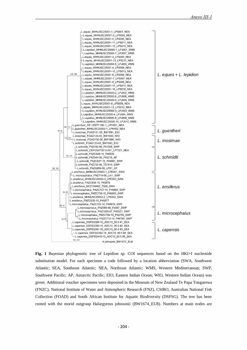
Anexo III-1
- 204 -
Fig. 1 Bayesian phylogenetic tree of Lepidion sp. COI sequences based on the HKI+I nucleotide
substitution model. For each specimen a code followed by a location abbreviation (SWA, Southwest
Atlantic; SEA, Southeast Atlantic; NEA, Northeast Atlantic; WMS, Western Mediterranean; SWP,
Southwest Pacific; AP, Antarctic Pacific; EIO, Eastern Indian Ocean; WIO, Western Indian Ocean) was
given. Additional voucher specimens were deposited in the Museum of New Zealand Te Papa Tongarewa
(FNZC), National Institute of Water and Atmospheric Research (FNZ), CSIRO, Australian National Fish
Collection (FOAD) and South African Institute for Aquatic Biodiversity (DSFSG). The tree has been
rooted with the morid outgroup Halargyreus johnsonii (BW1674_EU8). Numbers at main nodes are
L. eques + L. lepidion
L. guentheri
L. inosimae
L. schmidti
L. ensiferus
L. microcephalus
L. capensis

Anexo III-1
- 205 -
bootstrap percentages after 1000 replicates, based on genetic distances and Bayesian posterior probability
values.
Tab
le 2
Est
imat
es o
f gen
etic
dis
tan
ce o
ver
seq
uen
ce p
airs
wit
hin
and
bet
wee
n L
epid
ion
spec
ies
usi
ng t
he
Kim
ura
2-
par
amet
er m
odel
of
nu
cleo
tide
sub
stit
uti
on.

Anexo III-1
- 206 -
Tab
le 3
Bib
liogra
phic
com
pil
atio
n o
f th
e m
ain
mer
isti
c ch
arac
ters
of
no
min
al s
pec
ies
of
the
gen
us
Lep
idio
n.
Mer
isti
c: D
2 s
econd d
ors
al f
in r
ays,
A a
nal
fin
ray
s, G
R g
ill
rak
ers,
P p
ecto
ral
fin
ray
s
Dis
trib
uti
on:
M M
edit
erra
nea
n,
NA
No
rth
Atl
anti
c, N
P N
ort
h P
acif
ic,
OA
off
So
uth
Afr
ica,
SA
South
Atl
anti
c, S
P S
outh
Pac
ific

Anexo III-1
- 207 -
Table 4 Comparison between measurements and meristic features of L. eques from Atlantic waters and L.
lepidion from the Mediterranean Sea.
In marine fish species, interspecific variation in terms of genetic distance is generally
much higher than intraspecific variation, such that COI sequences may help to
discriminate among species. The interspecific genetic distance within the genus
Lepidion was 4.28%. The lowest average divergence between pairs of congeneric
species were 1.89% (range 1.56-2.51) for L. ensiferus and L. capensis and 1.98% (range
1.87-2.19) for L. guentheri and L. inosimae. These values were slightly lower than the
2% suggested as the minimal genetic distance value demanded for species
discrimination (Hebert et al. 2003, 2004). However, as pointed out by Ferguson (2002),
interspecific levels of divergence are variable among taxa, and a generalized 2% rule
cannot be applied to all species. Congeneric pairs in groups with normal rates of
mitochondrial evolution that show less than 2% divergence probably reflect short
histories of reproductive isolation. Some additional cases of low divergence may simply
be artefacts generated by flawed identifications, but other cases of congruence will
undoubtedly reflect mitochondrial introgression (Hebert et al. 2003). In fact, circa 15%
L. eques L. lepidion
Character Range n mean SD Range n mean SD
Total Length (mm) 170-355 36 135-217 20 As %HL
Eye diameter 29.0-37.8 36 34.1 2.2 27.6-35.3 20 30.7 1.8
Preorbital length 20.8-28.6 36 23.8 2.0 17.6-25.0 20 22.8 1.9 Postorbital length 38.8-44.7 36 42.2 1.3 44.4-51.3 20 46.5 1.6
Interorbital length 15.4-21.9 36 19.0 1.7 17.8-25.8 20 20.6 2.1
Barbel length 11.3-19.4 36 15.6 1.9 14.6-22.6 19 19.0 2.5 As %SL
Head length 19.4-23.9 36 21.9 1.0 21.2-25.3 20 23.6 1.1
2nd
Predorsal length 23-27 36 25.1 1.1 26.1-29.3 20 28.1 0.9
2nd
Dorsal base length 63.5-68.8 36 65.8 1.5 61.1-65.9 20 63.5 1.3 Anal base length 43.2-51.2 36 48.0 1.7 43.4-48.8 20 46.2 1.6
Caudal peduncle
length 2.4-5.9 36 4.4 0.7 2.9-7.0 20 4.4 1.0
Pectoral length 12.6-17.5 36 15.3 1.2 9.7-17.4 17 14.4 2.2
Ventral length 10.2-14.8 36 12.9 1.1 9.1-19.8 20 15.9 2.5
Body depth 14.5-23.4 36 19.1 2.4 15.7-22.8 20 18.8 2.1 Meristic features
1st Dorsal fin rays 4-5 36 4.4 0.5 4–5 20 4.7 0.4
2nd
Dorsal fin rays 51-59 36 55.9 1.9 53-57 20 55.1 1.2
Anal fin rays 47-54 36 50.2 1.6 45-51 20 48 1.5 Ventral fin rays 7-8 36 7.8 0.4 7–8 20 7.8 0.4
Pectoral fin rays 19-24 36 22 1.0 20-23 20 21.8 0.7
Gill rakers 18-21 36 19.6 1.0 18-23 20 20.1 1.1

Anexo III-1
- 208 -
of more than 5,000 barcoded fish species have congeneric distances <2.8% and 3.4%
have distances <1%, indicating clearly that, there is no absolute distance value that can
be employed as a hard criterion so that values above indicate interspecific divergence,
while those below are intraspecific (Ward et al. 2009). Thus, divergence averages of
1.11% were obtained within the genus Thunnus, 4.17% within the genus Squalus (Ward
et al. 2005) and 15.742% within genera of marine fishes from China (Zhang 2011).
These differences among genera probably reflect the average age of species divergence,
although within genera some species would be older than others (Ward et al. 2005).
Overall, the average genetic distance among congeneric species was 16-fold higher
than that of individuals within species. As a consequence of the variability within
genera, this metric also showed a great variability among taxa. The congeneric genetic
distance in all projects registered in the FISH-BOL database, containing over 7,000
species, is at least 30-fold higher than the conspecific one (Zhang & Hanner 2011). In
ornamental fishes, the average genetic distance between congeneric species was
approximately 26-fold higher than the within species variation (Steinke et al. 2009). In
coral reef fish larvae of the families Acanthuridae and Holocentridae, the divergence
among congeneric species was, on average, 20 to 87-fold higher than the divergence
between conspecific sequences (Hubert et al. 2010).
The L. schmidti haplotype from the NE Atlantic Ocean clustered together with the
haplotypes from the Pacific Ocean. This molecular coincidence reaffirms the presence
of L. schmidti in both oceans, as previously confirmed in a recent morphological study
(Arronte et al. 2011). The only L. guentheri haplotype from the NE Atlantic Ocean
clustered together with one haplotype of L. inosimae (FOAD131-05|BW-1691 EIO)
from the South Pacific Ocean, considered here as a misidentification of L. guentheri.
The possible presence of L. guentheri in the South Pacific Ocean suggests an Atlantic-
Pacific distribution for this species, similar to L. schmidti, although this issue needs to
be confirmed in future taxonomic studies.
The three haplotypes of L. ensiferus from the SE Atlantic Ocean clustered together
with L. ensiferus haplotypes from the same geographic area, but also with four
haplotypes of L. microcephalus from the SW Pacific Ocean, which were considered as
misidentifications. This fact could extend the known distribution area of L. ensiferus to
the SW Pacific Ocean.

Anexo III-1
- 209 -
Table 5 Comparison of three meristic characters of L. eques and L. lepidion from different geographical
areas, including data from Templeman (1970a,b) denoted by an asterisk.
The presence of this species is well documented in the SW Atlantic Ocean, the sub-
Antarctic islands of the Indian Ocean and the SE Pacific Ocean (Chiu et al. 1990;
Meléndez & Pequeño 1999; Reyes et al. 2009). Therefore, it is probable that L.
ensiferus has a circumglobal distribution in the Southern Hemisphere, and L. ensiferus
and L. microcephalus are probably two sympatric species in the SW Pacific Ocean.
Morphological identification of the Lepidion species requires the examination of a
number of features, which usually exhibit overlapping ranges, making accurate
identification difficult and producing some taxonomical confusion. There is need for
both a worldwide revision of the genus and a global identification key. In these cases,
the natural tendency of fish taxonomists is to consult regional checklists as an aid to
identification, although only a small number of species are usually included. However,
Species Area 2nd
Dorsal fin Range n mean SD
L. eques NW Atlantic* 55-60 15 57.67 1.45
Faroe Channel* 55-60 11 57.55 1.44
W Ireland* 56-58 12 56.75 0.75
Aviles canyon 53-59 10 56.6 1.9
Galician Bank 51-58 26 55.6 1.8
All areas 51-60 74 56.65 1.74
L. lepidion Mediterranean* 54-59 13 55.31 1.65
Balearic basin 53-57 20 55.1 1.2
All areas 53-59 33 55.18 1.38
Anal fin Range n mean SD
L. eques NW Atlantic* 51-54 14 52.57 0.76
Faroe Channel* 50-54 11 52.45 1.57
W Ireland* 50-53 12 52.25 0.97
Aviles canyon 49-54 10 51.2 1.6
Galician Bank 47-53 26 49.8 1.4
All areas 47-54 73 51.32 1.77
L. lepidion Mediterranean* 48-51 13 49.54 1.05
Balearic basin 45-51 20 48 1.5
All areas 45-51 33 48.6 1.61
Pectoral fin Range n mean SD
L. eques NW Atlantic* 21-25 15 22.93 0.96
Faroe Channel* 22-25 11 23 0.89
W Ireland* 22-24 12 22.75 0.87
Aviles canyon 21-23 10 22.3 0.67
Galician Bank 19-24 26 21.9 1.1
All areas 19-25 74 22.46 1.06
L. lepidion Mediterranean* 21-24 13 22.38 0.77
Balearic basin 20-23 20 21.8 0.7
All areas 20-24 33 22.06 0.79

Anexo III-1
- 210 -
if the real distribution of the Lepidion species is broader than currently known, this
could be a major source of potential misidentifications. For example, this seems to be
the case with L. schmidti, a species originally described from the Pacific Ocean
(Svetovidov 1936), erroneously misidentified as L. guentheri in the Northeast Atlantic
Ocean (Forster 1968), tentatively identified two years later as correct by Templeman
(1970a,b) and only recently confirmed in the latter area (Arronte et al. 2011). This could
also be the reason for the misidentifications of Lepidion spp. found in the BOLD
database.
The DNA barcoding results suggest the synonymy of L. eques and L. lepidion.
Morphologically, the taxonomic similarity between these two species has been
previously pointed out by several authors (Collett 1905, Roule 1919, Norman 1935,
Grey 1956 & Raimbault 1963). In his revision of the genus, Templeman (1970a,b)
stated that, in view of the great resemblances and the overlapping of meristic and mostly
of the morphometric character values, both species could be considered to have a
subspecific rather than a specific relationship, although, he concluded that it would be
unwise to make L. eques a synonym of L. lepidion.
These taxonomic uncertainties were not taken into account in subsequent
ichthyological publications (Cohen 1986a, Cohen et al. 1990), where L. lepidion and L.
eques were still considered valid and separate species.
In the literature both species of Lepidion have usually been separated on the basis of
the eye diameter in the head length, 3.1 to 3.6 times in L. lepidion and 2.6 to 3.1 times
in L. eques and by anal fin rays counts, 48-51 in L. lepidion and 50-54 in L.eques
(Cohen 1986a, Cohen et al. 1990). Our summary of comparative morphological and
meristic data (Table 4) extends, and for most characters overlaps previously published
ranges of values, invalidating them as specific diagnostic characters. For example, eye
diameter is contained 2.8-3.6 times in the head in L. lepidion and 2.6-3.4 in L. eques and
the number of anal fin rays are 45-51 in L. lepidion and 47-54 in L. eques. Significant
differences in those two morphometric variables analysed were only found in the mean
eye diameter. A significant latitudinal variation in this variable was also obtained in L.
eques. This may reflect that the observed interspecific differences might be due to a
location effect rather than to a species effect. Templeman (1970a) considered that the
morphological differences found between both species may be related to the warmer
and possibly also to the saltier environment of the Mediterranean Sea compared with the
North Atlantic Ocean. Likewise, according to our results, it is clear the presence of a

Anexo III-1
- 211 -
latitudinal gradient in the meristic counts of L. eques within the North Atlantic Ocean
(Table 5). The minimum average counts of the three meristic characters analysed were
found in the southern North Atlantic Ocean (Galician Bank), gradually increased further
northward. Moreover, these southern values are quite similar to the ones of the
Mediterranean L. lepidion.
Although geographical variation of morphometric and meristic characters is well
known in many fish species, they are poorly described for the genus Lepidion. Barlow
(1961) noted that lower meristic counts were generally found in lower latitudes
compared with higher latitudes. The Lepidion data followed the same trend, which
could explain the meristic differences found between the Atlantic and Mediterranean
specimens, which was erroneously used in the past to separate both species The number
of counts in a given meristic character is susceptible to the effects of both the
developmental stage and environmental factors, especially temperature variation with
latitude (Morris 1977). In previous studies of L. eques, an area lying to the west of
Ireland was the lowest latitude sampled (Templeman 1970a,b). Thus, in spite of
suspicions about the morphological similarities between L. eques and L. lepidion, the
results did not show the overlapping of characters caused by a latitudinal variation in L.
eques entirely. As Barlow (1961) pointed out, it is essential for the progress of
systematic ichthyology that the nature of the morphological variation in fishes is
properly understood.
Results from historical hydrographical cruises and climatological studies suggest the
existence of two veins of Mediterranean water in the NW of Spain, one on the slope
between the Galician Bank and the Iberian coast and the other recirculating to the west
of the Galician Bank (Ruiz-Villareal et al. 2006). The meristic similarities found
between the Mediterranean L. lepidion and the Atlantic L. eques on the Galician Bank
could be the result of both the environmental conditions of the Mediterranean water and
the possibility of gene flow between these two remote areas.
The COI DNA sequencing along with the morphological and meristic analysis
strongly suggests that there are no specific differences between the Atlantic L. eques
and the Mediterranean L. lepidion. Therefore, we propose L. eques as a junior synonym
of L. lepidion.
There has been a long controversy in the scientific community among advocates of
classical morphological and modern molecular taxonomic identification for a long time
(Ebach & Holdrege 2005). We agree with DeSalle et al. (2005), that genomic

Anexo III-1
- 212 -
information should be an active component of modern taxonomy, but DNA sequencing
should not be the sole source of information retrieval. In this context, the combination
of molecular and morphological data has become more frequent in more recent fish
taxonomic studies. The combination of these two types of analyses provides more solid
and reliable results, reducing the possibility of erroneous conclusions. Moreover, in our
opinion, DNA barcoding represents an extraordinary resource for the development of
new taxonomic hypotheses, which should be confirmed by reference to previously
published and/or future ichthyological studies.
References
Arronte JC, Bañón R, Quigley DTG, Pis-Millán JA, Heredia J (2011) New data on
Lepidion schmidti (Gadiformes: Moridae) from the north-east Atlantic Ocean.
Journal of Fish Biology, 79, 1709-1721.
Bañón R, Arronte JC, Heredia J, Pis-Millán JA (2010) First record of a specimen of
Lepidion guentheri (Giglioli, 1880) (Gadiformes: Moridae) with melanistic
coloration. Journal of Applied Ichthyology, 26, 602-605.
Barlow GW (1961) Causes and significance of morphological variation in fishes.
Systematic Biology, 10, 105-117.
Chiu TS, Markle DF, Meléndez R (1990) Moridae. In: Gon O and Heemstra PC (eds.)
Fishes of the Southern Ocean. Smith JLB Institute of Ichthyology,
Grahamstown, South Africa, pp 183-187.
Cohen DM (1986a) Moridae. In: Whitehead PJP, Bauchot M-L, Hureau J-C, Nielsen J,
Tortonese E (eds) Fishes of the Northeastern Atlantic and the Mediterranean,
Vol 2. UNESCO, Paris, pp 713-723.
Cohen DM (1986b) Moridae. In: Smith MM, Heemstra PC (eds) Smiths‟ sea fishes.
Macmillan, South Africa, Johannesburg, pp 326-328.
Cohen DM, Inada T, Iwamoto T, Scialabba N (1990) FAO Species Catalogue Vol 10.
Gadiform fishes of the world. Food and Agriculuture Organization of United
Nations, Rome.
Collett R (1905) Fiske indsamlede under “Michael Sars”s togter i Nordhavet 1900-
1902. Report on Norwegian Fishery and Marine Investigations, 2, 1-151.
Cowper TR (1956) A New Gadiform fish from the Continental Slope off Southeastern
Australia. Pacific Science, 10, 407-409.
Anexo III-1
- 213 -
DeSalle R, Egan MG, Siddall M (2005) The unholy trinity: taxonomy, species
delimitation and DNA barcoding. Philosophical Transactions of the Royal
Society B. doi:10.1098/rstb.2005.1722.
Ebach MC, Holdrege C (2005) More Taxonomy, Not DNA Barcoding. BioScience, 55,
822-823.
Felsenstein J (1985) Confidence limits on phylogenies: an approach using the bootstrap.
Evolution, 39, 783-791.
Ferguson JWH (2002) On the use of genetic divergence for identifying species.
Biological Journal of the Linnean Society, 75, 509-516.
Fitch JE, Barker LW (1972) The fish family Moridae in the eastern North Pacific with
notes on morid otoliths, caudal skeletons, and the fossil record. Fishery Bulletin,
70, 565-584.
Folmer O, Black M, Hoeh W, Lutz R, Vrijenhoek R (1994) DNA Primers for
amplification of mitochondrial cytochrome c oxidase subunit I from diverse
metazoan invertebrates. Molecular Marine Biology and Biotechnology, 3, 294-
299.
Forster GR (1968) Line-fishing on the continental slope. II. J Mar Biol Ass UK 48: 479-
483
Grey M (1956) The distribution of fishes found below a depth of 2000 meters.
Fieldiana Zoology, 36, 75–337.
Hasegawa M, Kishino H, Yano T (1985) Dating of the human-ape splitting by a
molecular clock of mitochondrial DNA. Journal of Molecular Evolution, 22,
160-174
Hebert PDN, Cywinska A, Ball SL, De Waard JR (2003) Biological identifications
through DNA barcodes. Proceedings of the Royal Society of London, 270, 313–
321.
Hebert PDN, Penton EH, Burns JM, Janzen DH, Hallwachs W (2004) Ten species in
one: DNA barcoding reveals cryptic species in neotropical skipper butterfly
Astraptes fulgerator. Proceedings of the National Academy of Sciences of the
United States of America, 101, 14812-14817.
Howes GJ (1991) Biogeography of gadoid fishes. Journal of Biogeography, 18, 595–
622.

Anexo III-1
- 214 -
Hubert N, Delrieu-Trottin E, Irisson JO, Meyer C, Planes S (2010) Identifying coral reef
fish larvae through DNA barcoding: A test case with the families Acanthuridae
and Holocentridae. Molecular Phylogenetics and Evolution, 55, 1195-1203.
Kimura M (1980) A simple method for estimating evolutionary rate of base
substitutions through comparative studies of nucleotide sequences. Journal of
Molecular Evolution, 16, 111–120.
Lloris D (1986) Ichofauna demersal y aspectos biogeográficos de la costa sudoccidental
de África (SWA/Namibia). Monografías de Zoología Marina, 1, 9-432.
Meléndez CR, Pequeño G (1999) New records of Morid fishes (Teleostei: Gadiformes)
from the southernmost tip of South America. Scientia Marina, 63, 465-467.
Moftah M, Abdel Aziz SH, Elramah S, Favereaux A (2011) Classification of Sharks in
the Egyptian Mediterranean Waters Using Morphological and DNA Barcoding
Approaches. PLoS ONE, 6, e27001.
Morris RW (1977) An Analysis of Some Meristic Characters of the Staghorn Sculpin
Leptocottus armatus Girard. Pacific Science, 31, 259-277.
Nakaya K, Amaoka K, Abe K (1980) A review of the genus Lepidion (Gadiformes,
Moridae) from the Northwestern Pacific. Japanese Journal of Ichthyology, 27,
41-47.
Nakamura I (1986) Moridae. In: Nakamura I (ed) Important fishes trawled off
Patagonia. Japan Marine Fisheries Resources Research Center, Tokyo, pp 104-
115
Norman JR (1935) Coast Fishes. Part I. The South Atlantic. Discovery Reports, 12, 1-
58.
Okamoto M, Sato N, Asahida T, Watanabe Y (2007) Pelagic juveniles of two morids
(Teleostei: Gadiformes: Moridae), Antimora microlepis and Physiculus
japonicus, from the western North Pacific. Species Diversity, 12, 17–27.
Okamoto M, Watanabe Y, Asahida T (2009) Descriptive morphology of pelagic
juvenile of Lepidion inosimae (Gadiformes: Moridae) collected from off
northeastern Japan. Ichthylogcal Research, 56, 76-81.
Paulin CD (1983) A revision of the family Moridae (Pisces, Anacanthini) within the
New Zealand region. National Museum of New Zealand Records, 2, 81-126.
Paulin CD (1984) First record of Lepidion inosimae (Günther) and L. schmidti
Svetovidov (Pisces: Moridae) from New Zealand. New Zealand Journal of
Zoology, 11, 59-62.

Anexo III-1
- 215 -
Paulin CD (1990) Moridae. In: Amaoka K, Matsuura K, Inada T, Takeda M, Hatanaka
H, Okada K (eds) Fishes collected by the R/V „„Shinkai Maru‟‟ around New
Zealand. Japan Marine Fisheries Resources Research Center, Tokyo, pp 149-157
Paulin CD, Roberts CD (1997) Review of the morid cods (Teleostei,
Paracanthopterygii, Moridae) of New Caledonia, southwest Pacific Ocean, with
description of a new species of Gadella. In: Séret B (ed) Résultats des
Campagnes MUSORSTOM, Memoires du Museum National d' Histoire
Naturelle, 174, 17-41.
Posada D, Crandall KA (1998) Modeltest: testing the model of DNA substitution.
Bioinformatics, 14, 817-818.
Raimbault R (1963) Notes sur certaines espèces ichthyologiques captureés au cours des
campagnes de l'Institut des Pêches en Méditerranée (1957-61). Revue des
Travaux de l'Institut Scientifique et Technique des Pêches Maritimes, 27, 161-
176.
R Development Core Team (2011) R: a language and environment for statistical
computing. R Foundation for Statistical Computing, Vienna, Austria. ISBN 3-
900051-07-0, URL http://www.R-project.org.
Reyes PR, Torres JP, Reyes EM (2009) Peces abisales del extremo austral de América
del sur (52°S-57°S), componentes de la fauna acompañante de la pesquería de
palangre del bacalao de profundidad (Dissostichus eleginoides Smitt, 1898).
Revista de Biología Marina y Oceanografía, 44, 59-65.
Roa-Varón A, Ortí G (2009) Phylogenetic relationships among families of Gadiformes
(Teleostei, Paracanthopterygii) based on nuclear and mitochondrial data.
Molecular Phylogenetics and Evolution, 52, 688-704.
Ronquist F, Huelsenbeck JP (2003) MrBayes version 3.0: Bayesian phylogenetic
inference under mixed models. Bioinformatics, 19, 1572-1574.
Roule L (1919) Poissons provenant des campagnes du yacht 'Princesse Alice' (1891-
1913) et du yacht 'Hirondelle II' (1914). Résultats des Campagnes scientifiques
du Prince Albert Ier de Monaco, 52, 1-191.
Ruiz-Villarreal M, Gonzalez-Pola C, Diaz del Rio G, Lavin A, Otero P, Piedracoba S,
Cabanas JM (2006) Oceanographic conditions in North and North West Iberia
and their influence on the Prestige oil spill. Marine Pollution Bulletin, 53, 220-
238.

Anexo III-1
- 216 -
Smith PJ, Steinke D, McMillan P, McVeagh SM, Stewart AL, Struthers CD (2008)
DNA database for commercial marine fish. New Zealand Aquatic Environment
and Biodiversity Reports, 22, 1-62.
Smith PJ, Steinke D, McMillan P, Stewart A, Ward RD (2011) DNA barcoding of
morid cods reveals deep divergence in the antitropical Halargyreus johnsoni but
little distinction between Antimora rostrata and Antimora microlepis.
Mitochondrial DNA, 22, 21-26.
Steinke D, Zemlak TS, Hebert PDN (2009) Barcoding Nemo: DNA-Based
Identifications for the Ornamental Fish Trade. PLoS ONE, 4, e6300.
Stöver BC, Müller KF (2010) TreeGraph 2: Combining and visualizing evidence from
different phylogenetic analyses. BMC Bioinformatics, 11, 7.
Svetovidov AN (1936) Lepidion schmidti, eine neue Fischart. Zoologischer Anzeiger,
113, 266-269.
Svetovidov AN (1937) Ueber die klassification der Gadiformes order Anacanthini.
Bulletin of the Academy of Sciences URSS, 4, 1281-1388.
Tamura K, Peterson D, Peterson N, Stecher G, Nei M, Kumar S (2011) MEGA5:
Molecular Evolutionary Genetics Analysis using Maximum Likelihood,
Evolutionary Distance, and Maximum Parsimony Methods. Molecular Biology
and Evolution, 28, 2731-2739.
Templeman W (1970a) A review of the morid fish genus Lepidion of the North Atlantic
with first records of Lepidion eques from the western North Atlantic. Journal of
the Fisheries Research Board of Canada, 27, 457- 498.
Templeman W (1970b) Additional tubular details of distributional meristic and
morphometric data of the paper: a review of the morid fish genus Lepidion of the
North Atlantic with first records of Lepidion eques from the western North
Atlantic (Templeman, 1970). Technical report - Fisheries Research Board of
Canada, 160 p
Trunov IA (1992) Morid cods from the southeast Atlantic (genera Lepidion,
Austrophycis, and Tripterophycis). Journal of Ichthyology, 32, 92-99.
Ward RD, Zemlak TS, Ines BH, Last PR, Hebert PDN (2005) DNA barcoding
Australia‟s fish species. Philosophical Transactions of the Royal Society B., 360,
1847-1857.
Ward RD, Hanner R, Herbert PDN (2009) The campaign to DNA barcode all fishes,
FISH-BOL. Journal of Fish Biology, 74, 329-356.
Anexo III-1
- 217 -
Zhang J (2011) Species Identification of marine fishes in China with DNA Barcoding.
Evidence-Based Complementary and Alternative Medicine, 2011, 1-10.
Zhang JB, Hanner R (2011) DNA barcoding is a useful tool for the identification of
marine fishes from Japan. Biochemical Systematics and Ecology, 39, 31-42.

Anexo III-1
- 218 -
Table S1 Biometric and meristic raw data of L. eques and L. lepidion used in the morphological analysis.
Lepidion lepidion Balearic Basin
BIOMETRIC L (mm) L (mm) L (mm) L (mm) L (mm) L (mm) L (mm)
Total length 154 140 168 181 207 156 205
Standard length 144 132 157 167 190 143 189
Head length 35 32 38 39 48 33 46
Snout length 8 7 9 9 11 8 11
Postorbital length 16 15 17 18 22 15 21
Eye diameter 11 10 12 12 15 10 14
Interorbital length 8 6 8 7 9 7 9
Predorsal1 length 34 31 40 39 45 35 46
Predorsal2 length 39 36 46 46 53 41 53
Dorsal1 base length 2 3 3 4 5 3 5
Dorsal2 base length 94 85 98 107 119 90 119
Maxilla length 15 16 18 19 21 16 22
Anal base length 69 60 75 75 89 62 89
Pectoral length − 16 23 − 33 17 29
Ventral length 19 12 25 25 33 23 27
Preanal length 60 58 68 74 79 65 80
Caudal peduncle Length 7 6 7 7 12 10 9
Minimum height of caudal peduncle
3 2 3 3 3 2 3
Body depth 26 22 26 34 36 26 39
Body width 12 10 14 16 24 14 18
MERISTIC
First dorsal rays 4 4 5 5 4 5 5
Second dorsal rays 56 57 54 57 55 54 54
Anal rays 51 49 47 51 48 47 48
Pectoral rays 20 22 20 22 22 22 21
Ventral rays 7 7 8 7 8 8 8
Branchiostegal rays 7 7 7 7 7 7 7
Gillrakers in first arch 6+15 5+15 6+15 6+13 6+15 5+16 5+13

Anexo III-1
- 219 -
Lepidion lepidion Balearic Basin
BIOMETRIC L (mm) L (mm) L (mm) L (mm) L (mm) L (mm) L (mm)
Total length 178 136 183 217 199 211 180
Standard length 167 134 175 202 184 196 162
Head length 41 32 42 45 45 48 40
Snout length 10 7 10 11 11 12 9
Postorbital length 19 15 19 20 21 22 18
Eye diameter 12 10 13 14 13 14 13
Interorbital length 8 6 9 9 8 9 9
Predorsal1 length 41 33 45 50 46 49 40
Predorsal2 length 49 38 51 57 53 56 46
Dorsal1 base length 4 3 4 5 4 5 4
Dorsal2 base length 105 85 107 128 116 123 101
Maxilla length 19 14 20 21 20 22 18
Anal base length 74 62 77 93 85 89 72
Pectoral length 23 17 17 30 23 20* 23
Ventral length 27 23 21 31 30 29 32
Preanal length 75 57 77 82 80 85 70
Caudal peduncle Length 7 7 8 8 8 9 7
Minimum height
of caudal peduncle 3 2 3 3 3 4 3
Body depth 36 24 36 46 38 43 28
Body width 16 12 14 21 18 26 17
MERISTIC
First dorsal rays 5 5 4 4 5 5 5
Second dorsal rays 56 56 54 55 55 54 54
Anal rays 48 47 49 45 48 46 48
Pectoral rays 22 22 23 22 22 22 22
Ventral rays 8 8 8 8 8 8 8
Branchiostegal rays 7 7 7 7 7 7 7
Gillrakers in first arch 6+14 5+14 6+15 5+15 6+14 6+14 6+17
Anexo III-1
- 220 -
Lepidion lepidion Balearic Basin
BIOMETRIC L (mm) L (mm) L (mm) L (mm) L (mm) L (mm)
Total length 171 159 172 145 157 135
Standard length 159 146 162 138 145 127
Head length 34 31 39 31 34 29
Snout length 6 7 8 6 8 7
Postorbital length 16 15 18 16 16 14
Eye diameter 12 9 13 9 10 8
Interorbital length 8 8 8 7 7 6
Predorsal1 length 36 34 38 30 35 31
Predorsal2 length 43 39 45 36 41 37
Dorsal1 base length 4 4 4 4 4 3
Dorsal2 base length 104 96 101 91 92 81
Maxilla length 14 14 15 12 13 11
Anal base length 77 70 76 65 65 62
Pectoral length 22 24 26 24 22 22
Ventral length 24 26 31 26 26 22
Preanal length 65 63 69 55 62 52
Caudal peduncle Length 5 5 7 4 5 4
Minimum height
of caudal peduncle 3 2 3 3 2 2
Body depth 28 24 29 23 29 20
Body width 17 17 16 14 14 12
MERISTIC
First dorsal rays 5 5 5 5 5 5
Second dorsal rays 57 56 54 56 55 53
Anal rays 50 48 47 49 45 49
Pectoral rays 22 22 22 22 23 22
Ventral rays 8 8 8 8 8 7
Branchiostegal rays 7 7 7 7 7 7
Gillrakers in first arch 6+15 6+13 6+13 6+14 6+14 6+14
Anexo III-1
- 221 -
Lepidion eques Galician Bank
BIOMETRIC L (mm) L (mm) L (mm) L (mm) L (mm) L (mm) L (mm)
Total length 267 311 283 329 322 273 336
Standard length 245 291 265 308 296 255 312
Head length 56 64 58 68 67 61 72
Snout length 13 16 13 19 17 13 19
Postorbital length 24 27 24 28 28 27 30
Eye diameter 19 21 21 21 22 21 23
Interorbital length 12 14 11 13 14 12 14
Predorsal1 length 50 63 53 69 63 60 70
Predorsal2 length 60 74 65 78 72 67 78
Dorsal1 base length 7 7 6 6 7 5 6
Dorsal2 base length 164 188 174 199 197 163 205
Maxilla length 17 28 24 26 26 22 28
Anal base length 119 128 124 133 141 118 147
Pectoral length 37 51 43 48 46 40 52
Ventral length 29 39 33 44 41 32 42
Preanal length 100 123 109 134 121 106 124
Caudal peduncle Length 12 16 15 15 15 11 15
Minimum height
of caudal peduncle 5 5 5 5 5 5 6
Body depth 49 58 59 61 66 52 70
Body width 28 38 31 36 37 31 37
MERISTIC
First dorsal rays 4 4 4 4 4 4 4
Second dorsal rays 58 57 51 55 54 54 55
Anal rays 53 50 51 49 50 48 49
Pectoral rays 23 23 24 23 21 19 22
Ventral rays 7 7 8 7 7 8 7
Branchiostegal rays 7 7 7 7 7 7 7
Gillrakers in first arch 5+15 5+14 6+15 5+15 6+15 5+14 5+13

Anexo III-1
- 222 -
Lepidion eques Galician Bank
BIOMETRIC L (mm) L (mm) L (mm) L (mm) L (mm) L (mm) L (mm)
Total length 355 282 279 296 290 332 304
Standard length 330 256 259 271 269 305 285
Head length 77 56 58 58 62 71 62
Snout length 22 12 13 15 17 19 15
Postorbital length 33 24 25 24 27 29 27
Eye diameter 23 20 20 19 18 23 20
Interorbital length 15 12 11 12 13 13 12
Predorsal1 length 80 51 60 54 60 71 61
Predorsal2 length 87 59 69 63 70 82 72
Dorsal1 base length 5 6 6 6 6 7 6
Dorsal2 base length 211 175 167 182 172 196 184
Maxilla length 34 23 26 24 27 31 28
Anal base length 149 128 126 130 128 142 136
Pectoral length 51 44 42 43 42 48 45
Ventral length 36 33 37 34 37 45 42
Preanal length 141 101 102 107 115 129 114
Caudal peduncle Length 18 10 12 13 12 15 13
Minimum height
of caudal peduncle 6 5 5 5 5 6 5
Body depth 65 60 55 53 61 65 52
Body width 42 35 28 30 31 41 31
MERISTIC
First dorsal rays 4 4 4 5 4 4 4
Second dorsal rays 57 56 56 58 57 53 56
Anal rays 49 49 51 49 48 49 50
Pectoral rays 21 23 23 22 21 22 21
Ventral rays 7 8 8 8 7 7 7
Branchiostegal rays 7 7 7 7 7 7 7
Gillrakers in first arch 6+14 6+15 6+15 5+13 6+14 5+13 5+13

Anexo III-1
- 223 -
Lepidion eques Galician Bank
BIOMETRIC L (mm) L (mm) L (mm) L (mm) L (mm) L (mm) L (mm)
Total length 219 227 210 255 229 290 239
Standard length 199 210 194 236 211 268 217
Head length 42 47 38 53 46 57 48
Snout length 10 12 8 13 11 14 10
Postorbital length 18 20 16 23 20 24 21
Eye diameter 14 15 14 17 17 19 17
Interorbital length 7 9 8 9 9 11 9
Predorsal1 length 41 43 41 50 49 58 48
Predorsal2 length 47 53 48 61 57 66 55
Dorsal1 base length 4 4 4 5 4 5 4
Dorsal2 base length 132 137 127 152 134 180 142
Maxilla length 19 21 18 22 22 26 21
Anal base length 97 97 96 114 102 131 106
Pectoral length 26 33 28 35 31 37 32
Ventral length 23 27 27 32 28 34 28
Preanal length 76 84 75 94 85 109 87
Caudal peduncle Length 10 11 7 11 9 12 10
Minimum height
of caudal peduncle 3 3 3 4 4 5 4
Body depth 35 42 33 43 44 55 35
Body width 19 23 16 26 22 31 20
MERISTIC
First dorsal rays 4 4 5 5 4 5 5
Second dorsal rays 55 54 56 57 58 57 56
Anal rays 49 47 52 50 49 51 50
Pectoral rays 20 20 23 22 22 22 23
Ventral rays 8 8 8 8 8 8 8
Branchiostegal rays 7 7 7 7 7 7 7
Gillrakers in first arch 6+14 5+15 6+14 6+15 5+15 5+13 5+15

Anexo III-1
- 224 -
Lepidion eques Galician Bank
BIOMETRIC L (mm) L (mm) L (mm) L (mm) L (mm)
Total length 254 194 205 248 261
Standard length 234 183 189 231 245
Head length 52 37 40 52 53
Snout length 13 8 9 12 12
Postorbital length 21 15 17 23 22
Eye diameter 18 14 14 17 19
Interorbital length 8 7 7 11 9
Predorsal1 length 50 36 39 52 53
Predorsal2 length 58 42 45 58 61
Dorsal1 base length 5 4 4 5 5
Dorsal2 base length 156 123 128 155 162
Maxilla length 23 18 18 23 23
Anal base length 116 89 94 116 118
Pectoral length 34 23 25 36 33
Ventral length 32 21 23 31 30
Preanal length 93 70 74 90 95
Caudal peduncle Length 11 9 9 10 12
Minimum height
of caudal peduncle 4 3 3 4 4
Body depth 47 33 37 48 52
Body width 26 14 17 26 30
MERISTIC
First dorsal rays 5 5 5 5 5
Second dorsal rays 52 56 57 55 57
Anal rays 52 49 52 49 49
Pectoral rays 22 22 22 21 22
Ventral rays 8 8 8 8 8
Branchiostegal rays 7 7 7 7 7
Gillrakers in first arch 6+13 5+15 6+15 5+15 5+13

Anexo III-1
- 225 -
Lepidion eques Aviles canyon
BIOMETRIC L (mm) L (mm) L (mm) L (mm) L (mm) L (mm) L (mm)
Total length 230 272 238 230 265 275 235
Standard length 215 250 220 209 244 254 219
Head length 45 55 47 43 54 54 49
Snout length 11 12 10 10 12 12 12
Postorbital length 19 23 21 18 22 22 19
Eye diameter 15 20 16 15 20 20 18
Interorbital length 8 9 8 7 10 10 9
Predorsal1 length 48 56 49 47 51 56 50
Predorsal2 length 57 65 56 52 60 60 57
Dorsal1 base length 5 5 4 4 5 6 6
Dorsal2 base length 137 172 145 138 165 171 142
Maxilla length 17 23 20 20 27 24 21
Anal base length 107 120 103 104 125 121 105
Pectoral length 31 42 35 33 40 41 33
Ventral length 22 36 24 25 31 32 30
Preanal length 82 100 93 82 93 105 90
Caudal peduncle Length 9 10 9 8 9 9 9
Minimum height
of caudal peduncle 3 3 3 3 4 4 4
Body depth 33 47 34 34 45 42 36
Body width 19 26 22 19 25 29 21
MERISTIC
First dorsal rays 4 4 5 5 4 5 5
Second dorsal rays 57 56 58 59 58 53 54
Anal rays 51 51 51 54 53 52 49
Pectoral rays 21 22 23 22 23 22 22
Ventral rays 8 8 8 8 8 8 8
Branchiostegal rays 7 7 7 7 7 7 7
Gillrakers in first arch 5+13 5+14 6+15 5+14 6+14 5+14 6+15

Anexo III-1
- 226 -
Lepidion eques Aviles canyon
BIOMETRIC L (mm) L (mm) L (mm)
Total length 199 193 170
Standard length 180 177 165
Head length 39 36 32
Snout length 9 9 7
Postorbital length 17 15 13
Eye diameter 13 12 12
Interorbital length 8 6 7
Predorsal1 length 41 40 36
Predorsal2 length 47 45 40
Dorsal1 base length 5 4 3
Dorsal2 base length 117 118 105
Maxilla length 17 17 13
Anal base length 85 89 76
Pectoral length 27 27 21
Ventral length 25 23 19
Preanal length 75 69 63
Caudal peduncle Length 6 6 4
Minimum height
of caudal peduncle 3 3 2
Body depth 30 28 24
Body width 18 16 13
MERISTIC
First dorsal rays 5 4 5
Second dorsal rays 58 57 56
Anal rays 52 50 49
Pectoral rays 23 22 23
Ventral rays 8 8 8
Branchiostegal rays 7 7 7
Gillrakers in first arch 5+15 5+14 6+14
Anexo III-1
- 227 -
Anexo III-2
- 228 -
ANEXO III-2
Bañón, R., Arronte, J.C., Isbert, W., Coscelli, G. & Sánchez, F. 2014. Melanic hyper-
pigmentation in the genus Lepidion (Gadiformes: Moridae). Cybium, 38 (3): 231-234.
Anexo III-2
- 229 -
Abstract
Two cases of melanic hyper-pigmentation in Lepidion lepidion are reported from two
localities in Spanish Atlantic waters. A bibliographic search revealed the occurrence of
this chromatic anomaly in another two Lepidion specimens, the first of them reported in
the late 19th century. Macroscopically, the colour abnormality was characterized by the
presence of numerous cutaneous irregular dark patches over the head, body and fins.
Microscopically, melanosis corresponds with hyperplasia of dermal melanophores.
Although the cause of the hyperplasic proliferation of pigmented cells could not be
determined, possible aetiologic agents were proposed. This is the first histopathological
study of a melanic specimen of the genus Lepidion.
INTRODUCTION
Pigmentation and integumentary colours in fish are the result of a combination of
coloured substances or biochromes, contained in various pigmented cells or
chromatophores. There are three major chromatophore cell types: melanophores,
xantophores and iridophores (Fujii, 1993). Melanophores contain melanin, which gives
a brown or black colouration. In teleosts, melanophores are commonly located in the
dermis of the skin, forming a pigmented layer, but they can also appear in the epidermis
and hypodermis (Beeching et al., 2013). The pigmentation patterns are regulated by
several intrinsic physiological conditions (Quigley and Parichy, 2002) and they are also
influenced by numerous environmental stressors such as exposure to light and
ultraviolet ray, temperature, osmolarity and pH of the water, mechanical pressure and
nutrition (Greenwood et al., 2012).
Many fish species may develop skin pigment abnormalities both in wild or farming
conditions, mainly associated to melanophore disorders. Hyper-pigmentation is one of
these disorders, characterized by the occurrence of focal or generalized spots, patches or
bands of dark coloration (Groff, 2001; Simon et al., 2009). It has been commonly
observed associated with pathological conditions such as chronic inflammation,
hyperplasic or neoplastic proliferation of melanophores (Roberts, 2012; Lévesque et al.,
2013).
Skin lesions, including hyper-pigmentation, have received considerable attention in
the last few years, as they represent indicators of water pollution and/or otherwise
stressed aquatic environments (Vethaak and Jol, 1996). The purpose of this study is to
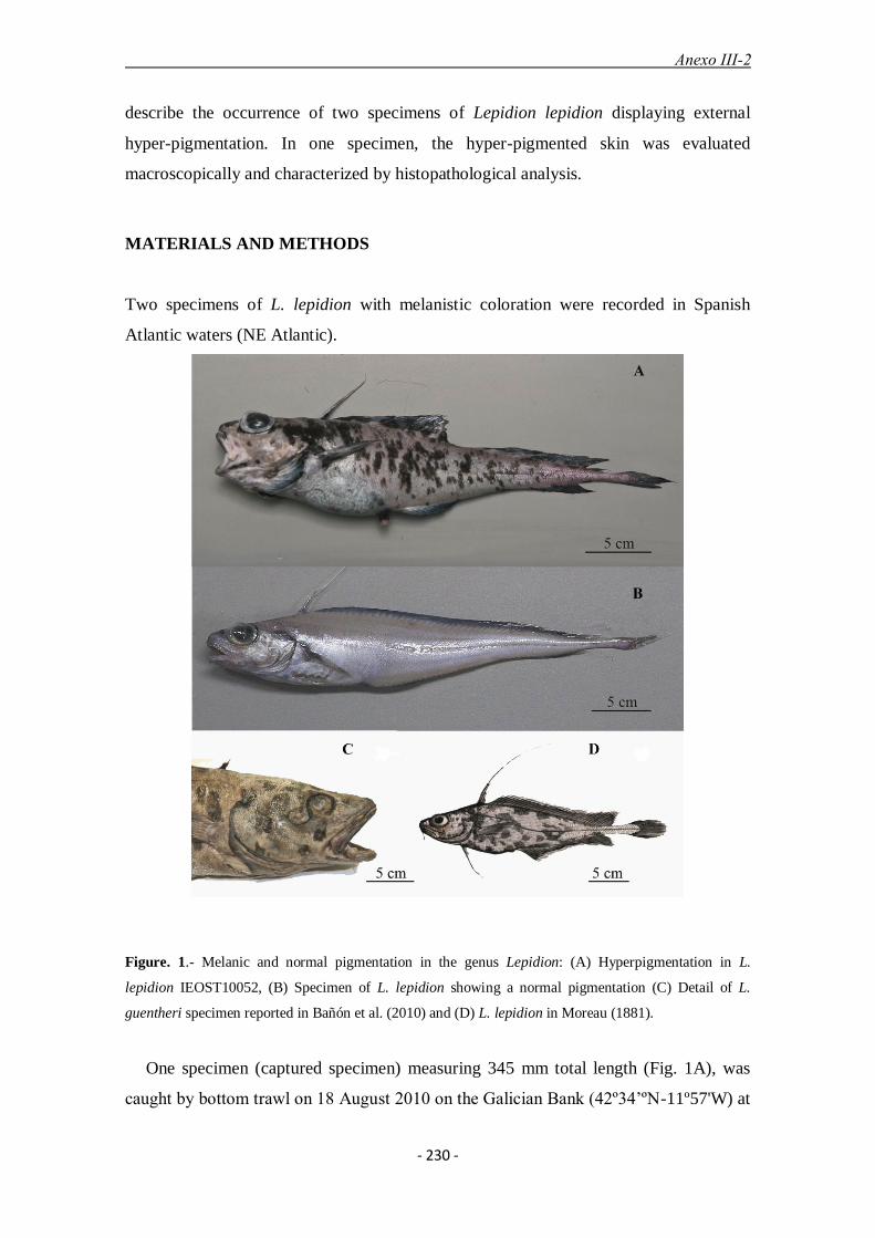
Anexo III-2
- 230 -
describe the occurrence of two specimens of Lepidion lepidion displaying external
hyper-pigmentation. In one specimen, the hyper-pigmented skin was evaluated
macroscopically and characterized by histopathological analysis.
MATERIALS AND METHODS
Two specimens of L. lepidion with melanistic coloration were recorded in Spanish
Atlantic waters (NE Atlantic).
Figure. 1.- Melanic and normal pigmentation in the genus Lepidion: (A) Hyperpigmentation in L.
lepidion IEOST10052, (B) Specimen of L. lepidion showing a normal pigmentation (C) Detail of L.
guentheri specimen reported in Bañón et al. (2010) and (D) L. lepidion in Moreau (1881).
One specimen (captured specimen) measuring 345 mm total length (Fig. 1A), was
caught by bottom trawl on 18 August 2010 on the Galician Bank (42º34’ºN-11º57'W) at
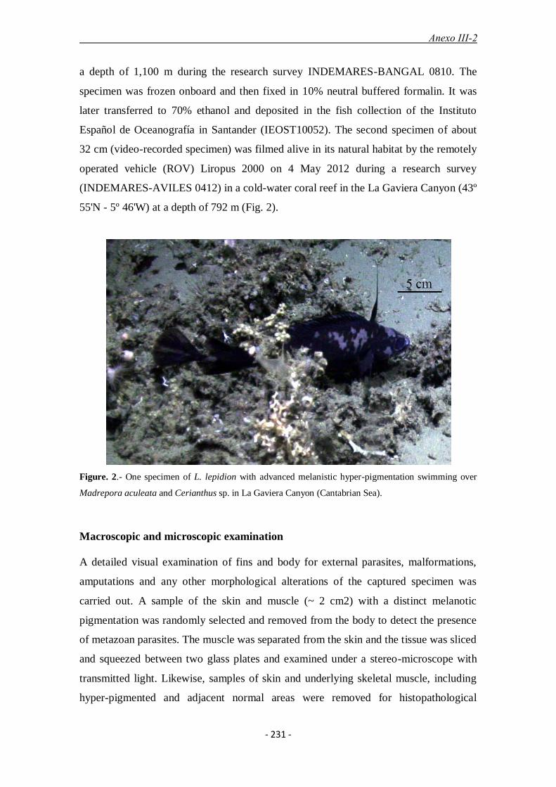
Anexo III-2
- 231 -
a depth of 1,100 m during the research survey INDEMARES-BANGAL 0810. The
specimen was frozen onboard and then fixed in 10% neutral buffered formalin. It was
later transferred to 70% ethanol and deposited in the fish collection of the Instituto
Español de Oceanografía in Santander (IEOST10052). The second specimen of about
32 cm (video-recorded specimen) was filmed alive in its natural habitat by the remotely
operated vehicle (ROV) Liropus 2000 on 4 May 2012 during a research survey
(INDEMARES-AVILES 0412) in a cold-water coral reef in the La Gaviera Canyon (43º
55'N - 5º 46'W) at a depth of 792 m (Fig. 2).
Figure. 2.- One specimen of L. lepidion with advanced melanistic hyper-pigmentation swimming over
Madrepora aculeata and Cerianthus sp. in La Gaviera Canyon (Cantabrian Sea).
Macroscopic and microscopic examination
A detailed visual examination of fins and body for external parasites, malformations,
amputations and any other morphological alterations of the captured specimen was
carried out. A sample of the skin and muscle (~ 2 cm2) with a distinct melanotic
pigmentation was randomly selected and removed from the body to detect the presence
of metazoan parasites. The muscle was separated from the skin and the tissue was sliced
and squeezed between two glass plates and examined under a stereo-microscope with
transmitted light. Likewise, samples of skin and underlying skeletal muscle, including
hyper-pigmented and adjacent normal areas were removed for histopathological

Anexo III-2
- 232 -
analysis. Fixed tissues were routinely processed and paraffin-embedded. Sections of 3-4
µm thickness were cut and stained with haematoxylin and eosin (H-E), periodic acid-
Schiff (PAS) and Fontana-Masson (FM) staining. Alternatively, additional sections
were bleached with 3% H2O2 for 24 h (in a humid chamber at room temperature)
before H-E stainings. Skin samples of three specimens displaying normal pigmentation
were used as a reference for normal histological structure.
RESULTS
Normal pigmentation
The typical pigmentation of L. lepidion is uniformly pale, varying from light brown to
grey-pink, with the fin extremities lightly pigmented (Fig. 1B).
Altered skin pigmentation
Macroscopic examination
The captured and video-recorded specimens of L. lepidion, both exhibited darkened skin
with evident hyper-pigmented areas, including the head, operculum and body surface. In
the captured specimen, lesions were characterized by generalized, multifocal dark
brown and black macules and spots with a smooth surface (Fig. 1A). Lesions were
variable in shape and size, varying from well-demarcated spots to irregular and diffuse
patches. Transverse sections of the body showed that hyper-pigmentation was restricted
to the skin and was not found deep in the musculature. In addition, the captured fish
exhibited a partial amputation on its dorsal profile, specifically in the middle of its
second dorsal fin. The video-recorded specimen exhibited a similar skin colour pattern,
but a higher proportion of skin surface was covered by hyper-pigmentation.
Microscopic examination
The parasitological examination did not reveal any parasites either on the skin or in the
muscular tissue. The histological examination of hyper-pigmented skin showed
hyperplasia of dermal melanophores (Fig. 3A). Pigmented cells were largely distributed
throughout the stratum laxum of the dermis, beneath the epidermis and above the scales,
but not extending into the deep dermis. They formed a thick, continuous and compact
pigmented row, parallel to the basement membrane (Fig. 3B). Demelanized samples
showed melanophores with rounded to fusiform nuclei and indistinguishable

Anexo III-2
- 233 -
cytoplasmatic edges (Fig. 3C). Mitotic figures were not observed. Staining with the FM
technique confirmed the presence of melanin granules in pigmented cells (Fig. 3D).
There was no evidence of inflammatory or necrotic changes. No bacterial, fungal or
parasites structures were observed in any of the analysed sections.
Figure. 3.- Microphotographs of hypermelanized skin sections. A, pigmented cell proliferation in the
superficial dermis (stratum laxum) (arrows); epidermis (ep), scale (sc), deep dermis (dd). H-E, bar=50
µm. Insert: distribution of melanophores (arrows) in normal pigmented skin. H-E, bar=50 µm. B,
hyperplasia of melanophores in superficial dermis forming a thick heavily pigmented layer beneath the
epidermis (arrow); epidermis (ep), scale (sc), deep dermis (dd). H-E, bar=50 µm. C, foci of hyperplasic
melanophores densely clustered. H-E, bar= 20 µm. D, Positive argentaffin reaction of melanin granules.
FM staining, bar=100 µm.
DISCUSSION
Following a recent revision of the genus, the Atlantic L. eques has been proposed as a
junior synonym of the Mediterranean L. lepidion (Bañón et al., 2013). Therefore, L.
lepidion is a deep-water species widely distributed in the North Atlantic Ocean and the
Mediterranean Sea.
Macroscopically, the anomalous colouration pattern was quite similar in both
specimens. A similar colouration pattern was previously reported in a specimen of the
congeneric L. guentheri from the Bay of Biscay (Bañón et al., 2010) (Fig. 1C) and in a
specimen of L. lepidion from the Mediterranean Sea (Moreau, 1881; Vinciguerra, 1883)
(Fig. 1D). Thus, the Moreau original drawing (1881, Vol. 3 p. 262), would appear to
Anexo III-2
- 234 -
represent the first documented case of melanosis in the genus Lepidion and one of the
first, if not the first, among marine fishes.
Microscopically, the histopathological examination of tissues revealed that the skin
melanosis corresponded with a severe hyperplasia of dermal melanophores, which
resulted in the darkened skin. However, the aetiology of melanophore hyperplasia could
not be established.
Hyperplasia is characterized by an increase in organ size or tissue involved that can
be caused by an excessive and/or prolonged stimulation of hormones or growth factors
on target cells, but also by inflammatory response to certain bacterial and viral
infections or physical agents, such as radiation or trauma (Cockerell and Cooper, 2002;
Sweet et al., 2012; Lévesque et al., 2013).
Melanophore hyperplasia seems to be a frequent cause of hyper-pigmentation in
fishes and has been described previously in other fish species, such as Sebastes sp.,
Pagellus acarne, Limanda limanda and Xiphophorus sp. (Gimenez-Conti et al., 2001;
Noguera et al., 2013; Ramos et al., 2013).
The microscopic examination showed neither dermal inflammatory changes nor
histological evidence of viral, bacterial, fungal or parasite infection. However, a
preceding inflammatory process cannot be ruled out because the inductor stimuli could
have been activated long before the specimen was examined.
Thus, the lesion observed in the second dorsal fin of the captured fish may represent
a sequel to a traumatic event, which may have been the initial stimulus that triggered the
proliferation of melanophores. Although aetiology was not considered in the original
publication, the specimen of L. guentheri with hyper-pigmentation reported by Bañón et
al. (2010) also showed a sequel scar as a result of a traumatic injury in the suborbital
area of the specimen's right eye (Fig. 1C). Unfortunately, the presence of wounds or
injuries in both Moreau’s drawing and the video-recorded specimen of L. lepidion could
not be confirmed.
Chromatic alterations in fish species related to traumas, wounds and injuries have
previously been reported in other fish species as Carassius auratus (Smith, 1931) and
flatfishes (Norman, 1934; Dahlberg, 1970).
The four compiled cases confirm the presence of melanic hyper-pigmentation within
the genus Lepidion. However, considering the relatively small number of melanic
specimens found to date, the prevalence of this condition in wild populations seems to
be very low. Nevertheless, specific attention to these anomalies is required in order to

Anexo III-2
- 235 -
achieve a more comprehensive knowledge about the occurrence of melanic hyper-
pigmentation in deep-water fish species.
REFERENCES
BAÑÓN R., ARRONTE J.C., HEREDIA J. & PIS-MILLÁN J.A., 2010.- First record of
a specimen of Lepidion guentheri (Giglioli, 1880) (Gadiformes: Moridae) with
melanistic coloration. J. Appl. Ichthyol., 26: 602-605.
BAÑÓN R., ARRONTE J.C., VÁZQUEZ-DORADO S., DEL RÍO J. & DE CARLOS
A., 2013.- DNA barcoding of the genus Lepidion (Gadiformes: Moridae) with
recognition of Lepidion eques as a junior synonym of Lepidion lepidion. Mol.
Ecol. Res., 13: 189-199.
BEECHING S.C., GLASS B.A. & REHOREK S.J., 2013.- Histology of melanic flank
and opercular color pattern elements in the Firemouth Cichlid, Thorichthys
meeki. J. Morphol., 274, 7: 743-749.
COCKERELL G.L. & COOPER B.J., 2002.- Disorders of cell growth and cancer
biology In: Mechanisms of Disease: A Textbook of Comparative General
Pathology (Slauson D.O. & Cooper B.J., eds), pp. 299-376. St. Louis, USA.
DAHLBERG M.D., 1970.- Frequencies of abnormalities in Georgia estuarine fishes.
Trans. Amer. Fish. Soc., 99: 95–97.
FUJII R., 1993.- Cytophysiology of fish chromatophores. Int. Rev. Cytol., 143, 191-255.
GIMENEZ-CONTI I., WOODHEAD A., HARSHBARGER J.C., KAZIANIS S.,
SETLOW R.B., NAIRN R.S. & WALTER, R.B., 2001.- A proposed
classification scheme for Xiphophorus melanomas based on histopathological
analyses. Mar. Biotechnol., 3, 1: S100-S106.
GREENWOOD A.K., CECH J.N. & PEICHELA C.L., 2012.- Molecular and
developmental contributions to divergent pigment patterns in marine and
freshwater sticklebacks. Evol. Dev., 14, 4: 351-362.
GROFF J.M., 2001.- Cutaneous biology and diseases of fish. Vet. Clin. North.Am. Exot.
Anim. Pract. 4, 2: 321-411.
LÉVESQUE M. P., KRAUSS J., KOEHLER C., BODEN C. & HARRIS M.P., 2013.-
New tools for the identification of developmentally regulated enhancer regions
in embryonic and adult zebrafish. Zebrafish 10, 1: 21-29.

Anexo III-2
- 236 -
MOREAU E., 1881.- Histoire naturelle des poissons de la France (Vol. 3). 698 p. Paris:
Masson.
NOGUERA P.A., FEIST S.W., BATEMAN K.S., LANG T., GRÜTJEN F. & BRUNO
D.W., 2013.- Hyperpigmentation in North Sea dab Limanda limanda. II.
Macroscopic and microscopic characteristics and pathogen screening. Dis.
Aquat. Org., 103: 25-34.
NORMAN J.R., 1934.- A systematic monograph of flatfishes (Heterosomata). Vol I:
Psettodidae, Bothidae, Pleuronectidae. 463 p. London: British Museum (Natural
History).
QUIGLEY I.K. & PARICHY D.M., 2002.- Pigment pattern formation in zebrafish: a
model for developmental genetics and the evolution of form. Microsc. Res.
Tech., 58: 442-455.
RAMOS P., VICTOR P. & BRANCO S., 2013.- Spontaneous melanotic lesions in
axillary seabream, Pagellus acarne (Risso). J. Fish Dis., 36, 9: 769-77.
ROBERTS R.J., 2012.- Fish pathology (4th edition). 590 p. Wiley-Blackwell.
SIMON T., JOYEUX J.C. & MACIEIRA R.M., 2009.- First record of partial melanism
in the coney Cephalopholis fulva (Perciformes: Epinephelidae). Braz. J.
Oceanogr., 57, 2: 145-147.
SMITH G.M., 1931.- The occurrence of melanophores in certain experimental wounds
of the goldfish (Carassius auratus). Biol. Bull., 61, 1: 73–84.
SWEET M., KIRKHAM N., BENDALL M., CURREY L., BYTHELL J. & HEUPEL
M., 2012.- Evidence of melanoma in wild marine fish populations. PLoS ONE,
7: e41989.
VETHAAK A.D. & JOL J.C., 1996.- Diseases of flounder Platichthys flesus in Dutch
coastal and estuarine waters, with particular reference to environmental stress
factors. I. Epizootiology of gross lesions. Dis. Aquat. Org., 26: 81-97.
VINCIGUERRA D., 1883.- Resultati Ittiologici delle crociere del "violante". Annali
Mus. civ. Stor. nat. Genova, 18: 465-590.

Anexo IV
- 237 -
ANEXO IV
Bañón, R., Arronte, J.C., Barros-García, D., Vázquez-Dorado, S. & de Carlos, A.
2013. Taxonomic study of Bathygadidae fishes (Gadiformes) from Atlantic Spanish
waters combining morphological and molecular approaches. Zootaxa, 3746 (4): 552–
566.

Anexo IV
- 238 -
Abstract From 2009 to 2011 eleven specimens belonging to four bathygadid species of
the family Bathygadidae were captured in two different locations in the northern waters
of Spain. The morphometric measurements and meristic characters of these specimens
are given. The specimens were identified as belonging to the genera Gadomus Regan,
1903, and Bathygadus Günther, 1878, including the following species: Gadomus dispar
(Vaillant, 1888), Gadomus longifilis (Goode & Bean, 1885), Gadomus arcuatus (Goode
& Bean, 1886) and Bathygadus melanobranchus Vaillant, 1888. As a result, a new
northern limit of distribution of G. arcuatus from the northeastern Atlantic is reported.
The first molecular identification and genetic interrelationships of Bathygadidae
species, based on the mitochondrial COI nucleotide sequences -DNA barcodes- is
reported. Sequences corresponding to specimens from the same species were identical
and the overall mean genetic diversity (uncorrected p-distance) was 0.096 ± 0.008.
Based on a morphological and meristic examination of the specimens, as well as on the
available literature, an updated key of the members of the family Bathygadidae from the
north-eastern Atlantic Ocean is provided.
Introduction
The grenadiers or rattails, traditionally included in the family Macrouridae, are now
divided in three families: Bathygadidae, Macrouridae and Trachyrincidae (Howes,
1989; Roa-Varón & Ortí, 2009). The family Bathygadidae, also known as bathygadids,
contains two genera, the genus Bathygadus, with 13 species, and the genus Gadomus,
with about 13 species. Bathygadids show a worldwide distribution from tropical to
subtropical seas, at depths of between 100 and 3,000 m. They can be found in the
Atlantic Ocean, between 40ºN and 40ºS, principally along the African continental slope,
in the west confined to the Gulf of Mexico and Caribbean Sea, extending east to the
mid-oceanic ridge; the Indian Ocean, the Natal and Somali basins, the Arabian Sea and
the Bay of Bengal; the Pacific Ocean, the Philippine Seas, the southern slope of Japan,
north of New Zealand, the Hawaiian islands and from the Sala-y-Gomez Ridge (Howes,
1991; Sazonov & Iwamoto, 1992).
Bathygadids are characterized by the presence of two dorsal fins, with the second
beginning immediately behind the first without a pronounced gap; first dorsal fin with
two spinous rays, the first one rudimentary and the second one smooth and flexible;
dorsal rays are longer than anal rays; 20 or more lathlike long outer gill rakers appear on
the first arch; 7 branchiostegal rays; no membrane restricts the first gill slit; 8-10 pelvic

Anexo IV
- 239 -
fin rays; the caudal fin is absent; there are no spinules on the scales; the swim bladder
has two or four retia mirabilia; the mouth is large and terminal and there is no
protruding snout (Marshall & Iwamoto, 1973; Iwamoto & Graham, 2001). Differences
in functional morphology between bathygadids and macrourids seem to be related with
their respective strategies for capturing prey. As a general rule, bathygadids, as pelagic
feeders, have a wide mouth and terminal and dorsal rays longer than the anal ones
whereas macrourids, as benthic to benthopelagic feeders, have subterminal or inferior
mouths and longer anal rays than the dorsal ones (Marshall, 1965; McLellan, 1977).The
taxonomic position of the Bathygadids is controversial, being a subject of scientific
debate. Some authors assigned this group to the suborder Macrouroidei (Iwamoto,
1989) whereas others to the suborder Gadoidei (Howes, 1989; Howes & Crimmen,
1990). On the other hand, Bathygadus and Gadomus have been traditionally constituting
the subfamily Bathygadinae of the family Macrouridae (Marshall & Iwamoto, 1973;
Maul, 1976). However, based on morphological and molecular evidences, this group
has been recognized at the family level (Howes & Crimmen, 1990; Iwamoto & Graham,
2001; Shao et al. 2008).
Morphologically, the bathygadids are chiefly distinguished from macrourids in
having the combination of second dorsal fin better developed (higher) than the anal fin;
the outer gill rakers long and slender (vs tubercular); the first gill slit no restricted by
folds of skin connecting the dorsal and ventral regions of the arch with the operculum, a
terminal mouth, viliform teeth, the body scales without spinules and all members have
seven branchiostegal rays (Iwamoto & Anderson, 1994). Molecular data based on
mitochondrial and nuclear DNA sequence analysis (average p-distance calculations)
among the Gadiformes also suggest that Bathygadinae could be ranked at the family
level (Roa-Varón & Ortí, 2009).
Recent morphological and genetic analyses support that bathygadids are basal to the
other grenadiers (Endo, 2002; Satoh et al. 2006; Iwamoto 2008; Roa-Varón & Ortí,
2009). However, the fossil records might imply that Macrouridae (with Nezumia
lindsay) is the oldest and probably most basal group, whereas Bathygadidae (the oldest
representative is Bathygadus novus from the Late Eocene of Italy) might be more
derived (Kriwet & Hecht 2008).
Differences among cytochrome oxidase c subunit I (COI) mitochondrial gene
sequences from distinct species can be used as a barcode in order to facilitate
identification of species, highlight cases of range expansion for known species, flag

Anexo IV
- 240 -
previously overlooked species and enable identifications where traditional methods
cannot be applied (Hebert et al. 2003). The analysis is focused on approximately 650
base pairs at the 5´end of the COI gene and the benefits in facilitating the identification
of species have been extensively proved for marine fish (Ward et al. 2009).
DNA barcoding data from bathygadid fishes are scarce in the ichthyiological
literature and only a few species have been barcoded until now. A barcode from
Bathygadus antrodes (Jordan & Starks, 1904) was obtained during the course of the
complete sequencing of a mtDNA genome in order to illustrate the phylogenetic
relationships among grenadier fishes by comparing the arrangement of their
mitochondrial genes (Satoh et al. 2006). In the largest COI database of macrourid fishes
of New Zealand, composed of 27 species, a barcode from the filamentous rattail
Gadomus aoteanus McCann & McKnight, 1980 is also mentioned (Smith et al. 2008).
At the moment of writing this paper, there are no published COI sequence records of
Gadomus and only five records of Bathygadus can be found in the BOLD database
(URL: http://v3.boldsystems.org/ accessed September 26, 2013), representing 3 species:
B. antrodes, B. favosus Goode & Bean,1886 and B. melanobranchus.
Taxonomic revisions of bathygadids have been previously carried out (Iwamoto,
1970; Marshall & Iwamoto, 1973; Howes & Crimmen, 1990; Iwamoto & Anderson,
1994). In the eastern Atlantic Ocean, the specific composition from the western Africa
waters has been recently updated, reporting seven bathygadid species, four Gadomus:
G. dispar, G. longifilis, G. arcuatus and G. capensis (Gilchrist & von Bonde, 1924) and
three Bathygadus: B. melanobranchus, B. macrops Goode & Bean, 1885 and B. favosus
Goode & Bean (Sobrino et al. 2012); only three of them, G. dispar, G. longifilis and B.
melanobranchus reaching the Atlantic European waters northward (Quéro et al. 2003).
However, little is known about the distribution and abundance of these species in
Atlantic European waters and our knowledge is based only on a few scattered records.
The aim of the current paper is to revise the species composition of the family
Bathygadidae from the Atlantic northern waters of Spain combining both the
morphological analysis and the molecular DNA barcoding method.
Material and methods
Sample collection, species identification and morphological analysis
Anexo IV
- 241 -
A total of eleven specimens of the family Bathygadidae were caught between 2009 and
2011 during 4 research cruises carried out in the Galicia Bank and the Avilés Canyon in
north-eastern Atlantic Ocean (northern Spanish waters). All specimens were tentatively
identified and subsequently frozen on board. Once in the laboratory, identification of
specimens to the species level was carried out according to Marshall & Iwamoto (1973)
and Howes & Crimmen (1990). Measurements to the nearest mm and meristic
characters were determined mainly according to Marshall & Iwamoto (1973).
Muscle samples were removed from thawed individuals and stored in 90% ethanol.
The specimens were then fixed in 10% formalin, prior to their storage in 70% ethanol.
Voucher specimens were deposited in the Museo de Historia Natural da Universidade
de Santiago de Compostela (MHNUSC, Santiago de Compostela, Spain). Photographs
of specimens used in this study and DNA sequence data are available in the project
entitled ―Barcoding of the family Bathygadidae‖ (code BATGA) in the Barcode of Life
Database (BOLD).
DNA extraction, PCR amplification and sequencing
Total DNA was purified from 25 mg of muscle tissue taken from each specimen using
the spin-column protocol of the DNeasy Blood and Tissue Kit (QIAGEN). The standard
5´ barcoding region of the COI gene (ca. 650 bp) was amplified by PCR using primers
LCOI1490 and HCOI2198 (Folmer et al. 1994). The following reaction conditions were
applied: initial denaturation at 94 ºC for 3 min followed by 35 cycles of 94 ºC for 30 s,
annealing at 52 ºC for 45 s and 72 ºC for 1 min, with a final extension at 72 ºC for 7
min. Polymerase chain reaction mixtures contained 1 x reaction buffer (TaKaRa), 25
pmol of each primer, 0.2 mM of each dNTP, 2 mM MgCl2, 0,25 U ExTaq DNA
Polymerase (TaKaRa) and 50-100 ng of template DNA. PCR reaction products were
visualized on 1.2% agarose gels (Seakem LE Agarose) stained with ethidium bromide
and, due to the specificity of the results, purified directly with ExoSAP-IT (USB)
following the manufacturer´s instructions. DNA sequencing reactions were carried out
in the direct and reverse senses using the same primers and the BigDye Terminator v3.1
Cycle Sequencing Kit (Applied Biosystems). The resulting products were resolved on
an ABI 3130 Genetic Analyser and the consensus sequences were obtained after
assembling the direct and reverse traces with SeqScape v2.5.
Sequence alignment and phylogenetic analysis
Phylogenetic and molecular evolutionary analyses were conducted in MEGA version 5
(Tamura et al., 2011). Twelve COI partial nucleotide sequences and their deduced

Anexo IV
- 242 -
amino acid alignments were built with the Alignment Explorer using the MUSCLE
program (Edgar, 2004). The number of base differences per site between sequences (p-
distance) served as genetic divergence estimation and was applied for the comparison of
pairs of haplotypes in general and also within and between congeners. The evolutionary
history among the bathygadid COI sequences was inferred by using the Maximum
Likelihood (ML) method based on the Hasegawa-Kishino-Yano model (Hasegawa et
al., 1985). Initial tree(s) for heuristic search were obtained automatically by applying
Nieghbor-Join and BioNJ algorithms to a matrix of pairwise distances estimated using
the Maximum Composite Likelihood (MCL) approach, and then selecting the topology
with superior log likelihood value. A discrete Gamma distribution was used to model
evolutionary rate differences among sites (G parameter = 0.1660). Codon positions
included were 1st+2nd+3rd+Noncoding. The species and gene sequences included in
the phylogenetic analysis are listed in the Table 1. For comparisons, the data set was
completed with a sample of G. arcuatus from the Canary Islands (28º 08,077' N, 14º
37,903' W) and barcodes of B. antrodes from Japan (GenBank Accession No
NC008222) and B. favosus (BIN BOLD: AAW2815) from the North Atlantic Ocean.
Sequences in BOLD of B. melanobranchus (MAECO390-09 and MAECO391-09) were
rejected of this analyses due to high genetic divergence found, which seems indicate
that they could be wrongly named. The barcode from a voucher specimen representing
the Atlantic cod Gadus morhua Linnaeus, 1758 (GenBank Accession No EU752090)
was used as outgroup in order to root the ML tree.
TABLE 1. Species used in the present study and gene sequences included in the phylogenetic analysis.
Species Location Sample ID BOLD
specimen
no.
GenBank accession
no.
Gadomus dispar Galicia Bank GAD001 BATGA003-13 KC959895
Galicia Bank GAD002 BATGA004-13 KC959900 Galicia Bank GAD003 BATGA005-13 KC959899
Galicia Bank GAD004 BATGA006-13 KC959898
Aviles Canyon GAD005 BATGA007-13 KC959897 Galicia Bank GAD006 BATGA008-13 KC959896
Gadomus longifilis Galicia Bank GAL001 BATGA009-13 KC959903
Galicia Bank GAL002 BATGA010-13 KC959901
Galicia Bank GAL003 BATGA011-13 KC959902 Gadomus arcuatus Aviles Canyon GAC001 BATGA002-13 KC959894
Canary Islands GAC002 BATGA012-13 KC959893
Bathygadus melanobranchus
Galicia Bank BGN001 BATGA001-13 KC959892

Anexo IV
- 243 -
Results
Genetics
Twelve COI DNA sequences were obtained from four different species of bathygadids
caught in the Galicia Bank, the Avilés Canyon and the Canary Islands: B.
melanobranchus (1 sequence), G. arcuatus (2 sequences), G. dispar (6 sequences) and
G. longifilis (3 sequences). The alignment of 651 nucleotides revealed the presence of
542 conserved and 109 variable sites from which 76 were parsimony informative (i.e.
containing at least two types of nucleotides and at least two of them occurring with a
minimum frequency of two) while 33 positions corresponded to singletons. Regarding
the 217 putative amino acid positions all but two were identical with the exception of
V138 (codon GUU) and T152 (codon ACC) in Bathygadus replaced by I138 (codons
AUC or AUU) and I152 (codons AUU or, AUC) in Gadomus.
The values of number of nucleotide differences per site (uncorrected p-distance)
between haplotypes from the specimens of the family Bathygadidae are shown in Table
2.
TABLE 2. Number of nucleotide differences per site (uncorrected p-distance) from averaging over all
COI haplotype pairs between bathygadids. Standard error estimates are shown above the diagonal and
were obtained by a bootstrap procedure (100 replicates).
B.
antrodes
B.
favosus
B.
melanobranchus
G.
arcuatus
G.
dispar
G.
longifilis
B. antrodes1 0.009 0.010 0.012 0.012 0.012
B. favosus2 0.051 0.009 0.013 0.013 0.012
B. melanobranchus 0.060 0.057 0.012 0.011 0.011
G. arcuatus 0.123 0.121 0.124 0.009 0.010
G. dispar 0.114 0.123 0.108 0.084 0.010
G. longifilis 0.109 0.106 0.103 0.071 0.084 1GenBank Accession No. NC008222.
2BIN BOLD:AAW2815 (MAECO389-09)
Sequences obtained from G. arcuatus, G. dispar and G. longifilis, produced only one
haplotype each. The mean overall distance (d ± S.E.) value among bathygadid
haplotypes was 0.096 ± 0.008. The within group mean distance was 0.056 ± 0.008 for
Bathygadus and 0.080 ± 0.009 for Gadomus. The group mean distance between the two
genera was 0.115 ± 0.010. The highest divergence occurred between B.

Anexo IV
- 244 -
melanobranchus and G. arcuatus (d = 0.124 ±0.012) while the lowest was between B.
antrodes and B. favosus (0.051 ± 0.009).
ML analysis was conducted with the HKY+G model of nucleotide substitution and
produced a phylogenetic tree showing that all species formed statistically well-
supported and coherent clades (Fig. 1). Two separated branches representing the two
genera of the family Bathygadidae can be observed. Regarding the sequences obtained
in this investigation, the various Gadomus sequences formed one clade and the only B.
melanobranchus sequence formed a second clade together with the congeneric ones
from B. antrodes and B. favosus mined from the databases. All sequences previously
assigned by taxonomy at the species level formed monophyletic clades with high
bootstrap values.
FIGURE 1. Molecular phylogenetic analysis of bathygadid COI barcoding sequences by Maximum
Likelihood method. For each specimen a code followed by a location abbreviation (NEA, Northeast
Atlantic) was given. Voucher specimens were deposited in the Museo de Historia Natural da
Universidade de Santiago de Compostela (MHNUSC) and Instituto Español de Oceanografía de Canarias
(IEOSC). A Gadus morhua sequence (EU752090) was employed as out-group. The percentage of trees in
which the associated taxa clustered together is shown above the branches. The scale bar represents 1 fixed
mutation per 10 nucleotide sequence positions.
Taxonomic descriptions
Family BATHYGADIDAE

Anexo IV
- 245 -
Genus Gadomus Regan, 1903
Gadomus dispar (Vaillant, 1888): Fig. 2.
Hymenocephalus dispar Vaillant, 1888: 221, Pl. 24 (Fig. 1). Off Morocco, 33°43'N,
9°02'W, station 20, depth 1105 meters. Holotype (unique): MNHN 1986-0551. Marshall
& Iwamoto, 1973: 518–530 (description, key); Howes & Crimmen 1990: 192–201
(description, key).
Material examined. MHNUSC 25004-1, 367 mm TL, 23th July 2009, Galicia Bank;
42º42.170 N—11º44.880' W; 765-766 m depth; MHNUSC 25004-2, 197 mm TL, 17th
August 2010, Galicia Bank; 42º39.968'N—11º43.327'W; 764-766 m depth; MHNUSC
25004-3, 171 mm TL, 21th August 2010, Galicia Bank; 42º42.960'N—11º43.000'W;
775 m depth; MHNUSC 25004-4, 187 mm TL, 21th
August 2010, Galicia Bank;
42º42.960'N—11º43.000'W; 775 m depth; MHNUSC 25004-5, 292 mm TL, 12th
May
2011, Avilés Canyon; 43º 54.970‘N—6º 15.250‘W; 1051 m depth; MHNUSC 25004-6,
260 mm TL, 3th
August 2011, Galicia Bank; 42º 49.180‘N—11º 46.890‘W; 909 m
depth.
Description. Body elongated and attenuated to the caudal peduncle; head small, 5.7-
6.7 times in total length; snout moderately acute, 4.3-5.8 into head; interorbital width
lower than horizontal eye diameter; barbel filamentous of moderate length, about as
long as the length of head, 0.8-1.2 in head length; dorsal, pectoral and ventral fins with
a single elongated ray; elongated second dorsal ray 1.6-2.7, elongated second pectoral
ray 1.7-2.2 and elongated first pelvic ray 0.9-2.0 in the head length. The main
morphometric and meristic characteristics are presented in Table 3.
Habitat and Distribution. Benthopelagic between 548 and 1,543 m depth in tropical
and subtropical North Atlantic (Marshall & Iwamoto, 1973; Sobrino et al. 2012).
Amphi-Atlantic distribution; in western Atlantic it occurs in Norfolk Canyon, eastern
Gulf of Mexico and the Caribbean Sea and in eastern Atlantic in the Cantabrian Sea,
Portugal, Morocco, Mauritania and Guinea-Bissau (Middleton & Musick, 1986;
Marques & Saldanha, 1998; McEachran & Fechhelm, 1998; Sánchez et al. 2008;
Sobrino et al. 2012).

Anexo IV
- 246 -
TABLE 3. Comparison of morphometric, meristic data and respective body proportions for specimens of
Gadomus dispar
Gadomus dispar MHNUSC
25004(1—6)
Marshall & Iwamoto
(1973)
Howes &Crimmen
(1990)
Total Length (mm) 171-367 — —
Head length (mm) 30-61 31-56 — As % TL
Head length 15.0-17.5 15-20 —
As % HL Eye diameter 24.6-29.0 26.8-31.6 27.6-29.5
Preorbital length 17.4-23.3 22.6-27.3 —
Postorbital length 48.4-56.5 — — Interorbital length 16.1-20.5 15.2-17.1 18.6-19.1
Upper jaw length 48.4-56.7 51.6-56.3 —
Barbel length 83.6-119.4 83.9-103.2 75.4-90.0
1stPredorsal length 95.7-119.4 112.9-117.7 —
2nd
Predorsal length 136.7-159.0 138.7-154.2 —
1st Dorsal base length 22.6-38.5 — —
Preanal length 200-233.3 192.8-206.4 — Length of longest ray of first
dorsal
161-270 126-135 —
Pectoral length 174.2-216 164-208 — Ventral length 93.3-108.7 96-116 —
Body depth 70.5-120 67.7-85.3 —
Meristic features
1st Dorsal fin rays II+9-11 12-13 II+9-11
Ventral fin rays 8 8 8
Pectoral fin rays 19-21 19-20 17-18
Gill rakers 4-5+19-21 4-5+20-21 4+20-21 Pyloric caeca >50 — 35+
FIGURE 2. Gadomus dispar from the north-east Atlantic Ocean, MHNUSC 25004-6, 260 mm total
length.
Gadomus longifilis (Goode & Bean, 1885): Fig. 3.
Bathygadus longifilis Goode & Bean, 1885: 599. Albatross station 2392,
28°47'30"N, 87°27'00"W, depth 724 fathoms. Syntypes: ?SU 9546 (1), USNM 37338
(2). Type catalog: Böhlke 1953:56. Parr, 1946: 8-17 (description, key); Iwamoto, 1970:

Anexo IV
- 247 -
327–352 (description, key); Marshall & Iwamoto, 1973: 518–530 (description, key);
Howes & Crimmen, 1990: 192–201 (description, key).
Material examined. MHNUSC 25005-1, 278 mm TL, 6th August 2011, Galicia
Bank; 42º 40.390‘N—11º 31.670‘W; 1,450 m depth; MHNUSC 25005-2, 291 mm TL,
6th August 2011, Galicia Bank; 42º 40.390‘N—11º 31.670‘W; 1,450 m depth;
MHNUSC 25005-3, 295 mm TL, 7th
August 2011, Galicia Bank; 42º 58.51‘N—11º
59.23‘W; 1,683 m depth.
Description. Body elongated and attenuated to the caudal peduncle; head small, 6.7-
7.7 times in total length; snout blunt, 3.7-4.4 times into head; interorbital width about
equal to horizontal diameter of orbit; long chin barbel present, strongly developed and
1.9-2.4 in head length; dorsal, pectoral and ventral fins with a single elongated ray,
elongated second dorsal ray 1.8-2.4, elongated second pectoral ray 2.0-2.3 and
elongated first pelvic ray 2.0-2.2 in the head length. The main morphometric and
meristic characteristics are presented in Table 4.
Habitat and Distribution. Benthopelagic in tropical and subtropical North Atlantic
between 520 and 2,165 m depth (Geistdoerfer, 1990). Amphi-Atlantic distribution; in
western Atlantic it occurs in West Greenland (a single specimen), off east coast of
Florida, Straits of Florida, Gulf of Mexico and Caribbean sea and in eastern Atlantic
from the northwest of Spain (Galicia), Portugal, Azores, Canary Islands, Morocco,
Mauritania and Gulf of Guinea (Marshall & Iwamoto, 1973; Maul, 1976; Geistdoefer,
1990; Jørgensen, 1996; Bañón et al. 2010; Sobrino et al. 2012).
FIGURE 3. Gadomus longifilis from the north-east Atlantic Ocean, MHNUSC 25005-3, 295 mm total
length.

Anexo IV
- 248 -
TABLE 4. Comparison of morphometric, meristic data and respective body proportions for specimens of
Gadomus longifilis.
Gadomus longifilis MHNUSC
25005(1—3) Parr
(1946) Iwamoto (1970)
Marshall & Iwamoto (1973)
Howes &
Crimmen
(1990)
Total Length (mm) 278-296 — 117-290 — —
Head length (mm) 38-41 — 19-45 25-46 —
As % TL
Head length 13.1-14.9 15-18 — ~15 — As % HL
Eye diameter 17.1-22.7 21-23 24-28 23.1-28.0 23.5-27.7
Preorbital length 22.7-26.8 28-30 26-31 26.3-28.9 — Postorbital length 54.5-57.9 — 46-53 — —
Interorbital length 21.1-22.7 23-25 21-28 21.1-25.0 19.7-24.8
Upper jaw length 56.1-60.5 60 57-65 52.6-60.0 — Barbel length 40.9-51.2 40-45 13-48 31.6-40.0 40.0-50.0
1stPredorsal length 112.2-113.6 — — 105.3-116.0 —
2nd
Predorsal length 152.6-156.8 — — 135.1-146.1 —
1st Dorsal base
length 34.2-39.0 30 — — —
Preanal length 197.6-202.6 — — 171.1-182.8 —
Length of longest ray of first dorsal
175.0-243.9 200 190 — —
Pectoral length 204.5-234.1 180 200 — —
Ventral length 204.5-217.1 160-170 250 — —
Body depth 87.8-94.7 — — 65.8-77.1 — Meristic features
1st Dorsal fin rays II+9-10 — II+8-10 9-11 II+9-10
Ventral fin rays 8 8 8 8 8 Pectoral fin rays 16-17 14-16 14-18 14-16 13-16
Gill rakers 7+29-31 — 7-8+26-
31
5-7+1+27-29 6-8+27-29
Pyloric caeca 9-12 10-12 9-13 — 5-12
Gadomus arcuatus (Goode & Bean, 1886): Fig. 4.
Bathygadus arcuatus Goode & Bean, 1886: 158. Off Martinique Island, West Indies,
Blake station 205, depth 334 fathoms. Holotype: MCZ 28007. Parr, 1946: 8-17
(description, key); Marshall & Iwamoto, 1973: 518–530 (description, key); Howes &
Crimmen 1990: 192–201 (description, key).
Material examined. MHNUSC 25006-1, 566 mm TL, 13th May 2011, Avilés
Canyon; 43º 57.850‘N—6º 28.050‘W; 1,450 m depth.
Description. Body elongated and attenuated to the caudal peduncle; upper profile to
first dorsal fin strongly inclined, with a pronounced hump-backed appearance; head
moderately large, 6.2 times in total length; snout 4.8 times into head; interorbital width
about equal to horizontal eye diameter and 5.4 times into head length; chin barbel
present and of moderate size, 0.7 in head length; mouth large and terminal jaws beyond
the posterior margin of the orbit; only one pelvic ray elongated but broken is patent, all
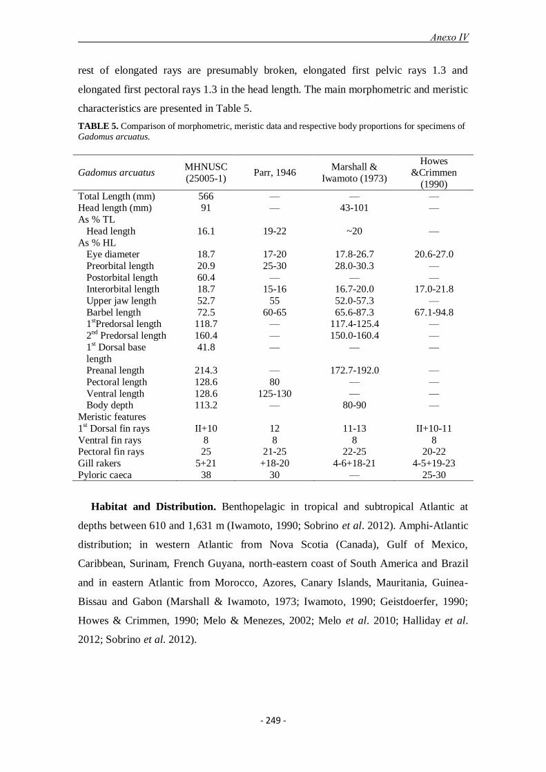
Anexo IV
- 249 -
rest of elongated rays are presumably broken, elongated first pelvic rays 1.3 and
elongated first pectoral rays 1.3 in the head length. The main morphometric and meristic
characteristics are presented in Table 5.
TABLE 5. Comparison of morphometric, meristic data and respective body proportions for specimens of
Gadomus arcuatus.
Gadomus arcuatus MHNUSC
(25005-1) Parr, 1946
Marshall &
Iwamoto (1973)
Howes &Crimmen
(1990)
Total Length (mm) 566 — — — Head length (mm) 91 — 43-101 —
As % TL
Head length 16.1 19-22 ~20 —
As % HL Eye diameter 18.7 17-20 17.8-26.7 20.6-27.0
Preorbital length 20.9 25-30 28.0-30.3 —
Postorbital length 60.4 — — — Interorbital length 18.7 15-16 16.7-20.0 17.0-21.8
Upper jaw length 52.7 55 52.0-57.3 —
Barbel length 72.5 60-65 65.6-87.3 67.1-94.8 1
stPredorsal length 118.7 — 117.4-125.4 —
2nd
Predorsal length 160.4 — 150.0-160.4 —
1st Dorsal base
length
41.8 — — —
Preanal length 214.3 — 172.7-192.0 —
Pectoral length 128.6 80 — —
Ventral length 128.6 125-130 — — Body depth 113.2 — 80-90 —
Meristic features
1st Dorsal fin rays II+10 12 11-13 II+10-11
Ventral fin rays 8 8 8 8 Pectoral fin rays 25 21-25 22-25 20-22
Gill rakers 5+21 +18-20 4-6+18-21 4-5+19-23
Pyloric caeca 38 30 — 25-30
Habitat and Distribution. Benthopelagic in tropical and subtropical Atlantic at
depths between 610 and 1,631 m (Iwamoto, 1990; Sobrino et al. 2012). Amphi-Atlantic
distribution; in western Atlantic from Nova Scotia (Canada), Gulf of Mexico,
Caribbean, Surinam, French Guyana, north-eastern coast of South America and Brazil
and in eastern Atlantic from Morocco, Azores, Canary Islands, Mauritania, Guinea-
Bissau and Gabon (Marshall & Iwamoto, 1973; Iwamoto, 1990; Geistdoerfer, 1990;
Howes & Crimmen, 1990; Melo & Menezes, 2002; Melo et al. 2010; Halliday et al.
2012; Sobrino et al. 2012).

Anexo IV
- 250 -
FIGURE 4. Gadomus arcuatus from the north-east Atlantic Ocean, MHNUSC 25006-1, 566 mm total
length.
Genus Bathygadus Günther, 1878
Bathygadus melanobranchus Vaillant, 1888: Fig. 5.
FIGURE 5. Bathygadus melanobranchus from the north-east Atlantic Ocean, MHNUSC 25007-1, 370
mm total length.
Description. Body elongated and attenuated to the caudal peduncle; head large, 6
times in total length; snout blunt, 4.1 times into head; mouth large and terminal, jaws do
not reaching the posterior margin of the orbit; snout as long as eye diameter and 4.1
times into head length; chin barbel absent; only first ventral ray slightly produced, 0.8 in
the head length. The main morphometric and meristic characteristics are presented in
Table 6.
Habitat and Distribution. Benthopelagic in tropical and subtropical Atlantic at
depths between 450 and 2,650 m, but generally from 700 to 1400 m (Marshall &
Iwamoto, 1973). Amphi-Atlantic distribution; in western Atlantic from the Gulf of
Mexico, Caribbean sea and off Suriname and in eastern Atlantic from the Irish
continental slope, Azores, Madeira, Canary Islands, Morocco, Mauritania, Guinea-

Anexo IV
- 251 -
Bissau, Senegal and Gabon (Farran, 1924; Marshall & Iwamoto, 1973; Sobrino et al.
2012). The records from South Africa were not included because they cannot be verified
(Howes & Crimmen, 1990).
TABLE 6. Comparison of morphometric, meristic data and respective body proportions for specimens of
Bathygadus melanobranchus.
Bathygadus
melanobranchus
MHNUSC
(25007-1)
Parr
(1946)
Iwamoto
(1970)
Marshall &
Iwamoto (1973)
Total Length (mm) 370 — 70-400 —
Head length (mm) 62 — — 28-89
As % TL Head length 16.8 — — 15-20
As % HL
Eye diameter 24.2 27-29 — 24.7-34.2
Preorbital length 24.2 — 25-33 24.7-29.2 Postorbital length 51.6 — 46-52 —
Interorbital length 29.0 — 25-35 24.7-33.9
Upper jaw length 54.8 54-57 51-60 46.1-56.5 1
stPredorsal length 111.3 — — 102.3-115.8
2nd
Predorsal length 151.6 — — 128.2-147.9
1st Dorsal base length 35.5 40 — —
Preanal length 195.2 — — 166.1-187.0
Length of longest ray
of first dorsal
51.6 50-55 < 50 —
Pectoral length 66.1 55-60 — — Ventral length 83.9 80-85 — —
Body depth 83.9 — — 71.9-80.3
Meristic features 1
st Dorsal fin rays II+10 — II+9-11 11-13
Ventral fin rays 8 — 8 7-8
Pectoral fin rays 16 — 16-20 16-19
Gill rakers 6+24 +21 6-7+21-24 5-7+0-1+21-23 Pyloric caeca 26 28 25-40 —
Key to species of Bathygadidae from the north-eastern Atlantic Ocean waters
(adapted from Iwamoto, 2003)
1a. Chin barbel very small or absent; no elongated fin rays in dorsal and pectoral fins
and only slightly elongated in the ventral fin..................................Genus Bathygadus (2)
1b. Chin barbel long, well developed; elongated fin rays in dorsal, pectoral and ventral
fins..................................................................................................Genus Gadomus (4)
2a.- Very small barbel present on chin; body integument relatively tough, not readily
torn; head bones strong; gill filaments pale......................................Bathygadus macrops

Anexo IV
- 252 -
2b. No barbel on chin; body integument weak, easily torn; head bones weak, easily
broken; gill filaments dusky or pale..............................................................................3
3a. Pelvic-fin rays 8; gill filaments dusky; interorbital width moderate, 4 or more times
into head length..................................................................Bathygadus melanobranchus
3b. Pelvic-fin rays 9; gill filaments pale; interorbital wide, 2.5-3.0 into head
.......................................................................................................Bathygadus favosus
4a. Two elongated rays in pelvic fin; pectoral-fin soft rays 20 to 28....Gadomus arcuatus
4b. One elongated ray in pelvic fin; pectoral-fin soft rays 14 to 21..................................5
5a. Gill rakers on lower limb of first arch 26 to 31; interorbital length 21-28% head
length; pectoral-fin soft rays 14 to 18; orbit 17.1-28.0% head length; 9-13 pyloric caeca
in adult specimens.............................................................................Gadomus longifilis
5b. Gill rakers on lower limb of first arch 19 to 21; interorbital length 15.2-20.5% head
length; pectoral-fin soft rays 17 to 21; orbit 24.6-31.6% head length; more than 50
pyloric caeca in adult specimens............................................................Gadomus dispar
Discussion
The latitudinal and depth distributions found in this study are in the same range of
previous records, with the exception of G. arcuatus, whose finding, in the Avilés
Canyon, constitutes a new northern limit of distribution from the eastern Atlantic
Ocean. The higher abundance of bathygadids in the eastern Atlantic seems to be
restricted to north-western Africa, specifically in the Morocco-Western Sahara area.
Merrett & Marshall (1981) found that B. melanobranchus is one of the most numerous
species of the fishes collected in this area, occupying a depth range of 734-1,017 m.
Ramos et al. (2006) reported B. melanobranchus and G. longifilis as two of the
dominant species in the global catch of deep demersal fauna in northern Morocco
between 500 and 2,000 m and Sobrino et al. (2012), pointed out that B. melanobranchus
and B. macrops are the most abundant macrourid fishes caught in the Morocco-Saharan
area.
The absence of both a long chin barbel and elongated fin rays separate the
Bathygadus from the Gadomus species (Howes & Crimmen, 1990). B. melanobranchus
can be separated from the other congeneric Atlantic species by the number of pelvic fin
rays (7-8 vs 9-10 in B. favosus), greater number of gillrakers (5-7+21-24 vs 5-6+19-21
in B. macrops) and wider interorbital length (24.5-33.9 vs 19.7-25.0 %HL in B.

Anexo IV
- 253 -
macrops) (Howes & Crimmen, 1990). The morphological measurements and counts of
our specimen, are in agreement with these ranges, confirming its correct identification
(Table 6).
In sampled specimens of Gadomus, the higher number of pectoral fins rays separate
G. arcuatus from the other two Gadomus species (25 vs 16-21). G. longifilis can be
easily differenced from G. dispar by the lower number of pectoral fin rays (16-17 vs 19-
21), greater gill raker counts on the lower limb of the first arch (29-31 vs 19-21), wider
interorbital length (21.1-22.7 vs 16.1-20.5 %HL), lower barbel length (40.9-51.2 vs
83.6-119.4 %HL) and lower number of pyloric caeca (9-12 vs more than 50). Also, G.
dispar can be differentiated from G. longifilis and G. arcuatus in having a greater eye
diameter and shorter head length (Howes & Crimmen, 1990). Our results confirm the
first diagnostic but not the second. The eye diameter was 24.6-29.0 %HL in G. dispar
compared to 17.1-22.7 in the other two congeners. However, G. dispar showed a greater
head length (15-17.5 %TL) than in the other two congeners (13.1-16.1%TL).The
morphometric and meristic data of Gadomus are generally in agreement, apart from
minor exceptions, with previous descriptions (Tables 3–6).
The presence of attenuated anterior dorsal, pectoral and pelvic fin rays is one of the
main distinctive characters in the genus Gadomus (Howes & Crimmen, 1990).
Nevertheless, due to their fragility, it is very frequent to find these rays partially or
completely broken. This fact can complicate the correct taxonomic identification and
also seems to be the cause of erroneous descriptions in the literature. In the first dorsal
fin of all bathygadids examined in this study, the second and flexible spinous ray was
the longest. In B. melanobranchus it is only slightly larger than the others rays, whereas
in the Gadomus species it is very elongated (broken in our specimen of G. arcuatus).
The presence of an enlarged dorsal ray in G. arcuatus has been described in some
specimens (Koefoed, 1927; Marshall & Iwamoto, 1973) but also its absence has been
observed in several individuals (Iwamoto, 1990). In G. dispar, the absence of an
elongated ray in the first dorsal and pelvic fins has been erroneously proposed as a
distinctive character (Iwamoto, 2003). The description of the holotype reported that
from state of preservation, it was not possible to determine if the second dorsal fin ray
was elongated or not. However, the presence of an elongated ray in pectoral and ventral
fins had already been described (Vaillant, 1888). In all of our specimens, as well as in
previous descriptions (Marshall & Iwamoto, 1973; Geistdoefer, 1986), the presence of
an elongated ray in dorsal, pectoral and ventral fins was observed.
Anexo IV
- 254 -
The second pectoral fin ray is elongated in the three Gadomus species (broken in our
specimen of G. arcuatus). This is in agreement with McEachran & Fechhelm (1998),
although some authors have described the first pectoral fin rays as the elongated one
(Maul, 1976; Geistdoerfer, 1986). After our revision, the following radial formulae with
respect to the position of the elongated fin ray is proposed: 2:2:1 for G. dispar and G.
longifilis and 2:2:1-2 for G. arcuatus, with reference to dorsal, pectoral and ventral fins,
respectively. The formula 2:2:1 could probably be applicable to the rest of the Gadomus
species, but this should be confirmed in future studies.
The counts of pyloric caeca are in agreement with those previously reported, 5-13 for
G. longifilis (Iwamoto, 1970; Howes & Crimmen, 1990), 25-40 for G. arcuatus (Cohen
et al. 1990; Howes & Crimmen, 1990) and 25-40 for B. melanobranchus (Iwamoto,
1986). For G. dispar, only a count of +35 has been reported (Howes & Crimmen, 1990).
Our specimens of G. dispar have numerous pale, long and thin pyloric caeca. Although
they were very difficult to count, they exceeded 50 in each count (about 58 in a
specimen of 292 mm TL). The number of pyloric caeca increases with the size (Howes
& Crimmen, 1990), which could be the main origin of the intraspecific differences
reported in literature.
Despite the fact that most of the specimens had been caught in different locations
and/or dates, the COI sequences from the six G. dispar, the three G. longifilis and the
two G. arcuatus are identical and represent a single barcode each. The zero value of the
intra-specific divergence in the Gadomus species may indicate that the COI gene
appears to be conserved in this genus, but this aspect should be proved in future
researches.
The bootstrap values of the ML phylogenetic tree support the formed clades,
validating the haplotype sequences as barcodes for the six species investigated.
Following the established procedure (Ward et al. 2009), it is provided for the first time a
barcode sequence for the species G. dispar, derived from six voucher specimens that
yield a single haplotype. The presence of various bathygadid sequences deposited in
BOLD Databases probably resembles other scientists initiatives related to the barcoding
of this or a similar group of species and will be reflected in the inclusion of these
sequences in future research papers. Although only 6 out of 26 (20.7 %) bathygadid
species are involved, this is the first approach to the genetic interrelationships into the
family Bathygadidae.

Anexo IV
- 255 -
The ‗Integrative taxonomy‘ is defined as the science that aims to delimit the units of
life‘s diversity from multiple and complementary perspectives (Dayrat, 2005). The
DNA barcoding technique has been successfully integrated with traditional
morphological analysis in the systematic studies of fishes (Baldwin & Weigt, 2012;
Bañón et al. 2013). Taxonomic studies including morphological and molecular data
could help to resolve identification mistakes and incongruities between DNA and
morphological results. Molecular tools have the potential to complement taxonomic
investigations by helping to reveal cryptic species, the identification of immature
specimens, and the clarification of problems of synonymy (Pires & Marinoni, 2010). On
the other hand, morphological analyses should be necessary to prove the correct
identification of all DNA barcoded species. Errors in identification are the primary
source of inaccuracies in FISH-BOL barcode data (Becker et al. 2011). Without verified
reference sequences from voucher specimens that have been authenticated by qualified
taxonomists, there is no reliable library for newly generated query sequences to be
compared with (Taylor & Harris, 2012).
There were no incongruities among morphological and molecular identification in
this study of the family Bathygadidae. The taxonomic identification supported the
genetic analysis and viceversa, which reinforces the resulting taxonomic identification.
References
Baldwin, C.C. & Weigt, L.A. (2012) A New Species of Soapfish (Teleostei: Serranidae:
Rypticus), with redescription of R. subbifrenatus and comments on the use of
DNA barcoding in systematic studies. Copeia, 1, 23–36.
Bañón, R., Villegas-Ríos, D., Serrano, A., Mucientes, G. & Arronte, J.C. (2010) Marine
fishes from Galicia (NW Spain): an updated checklist. Zootaxa, 2667, 1–27.
Bañón, R., Arronte, J.C., Vazquez-Dorado, S. del Rio, J.L. & de Carlos, A. (2013) DNA
barcoding of the genus Lepidion (Gadiformes: Moridae) with recognition of
Lepidion eques as a junior synonym of Lepidion lepidion. Molecular Ecology
Resources, 13, 189–199.
Becker, S., Hanner, R. & Steinke, D. (2011) Five years of FISH-BOL: brief status
report. Mitochondrial DNA, 22, 3–9.
Cohen, D.M., Inada, T., Iwamoto, T. & Scialabba, N. (1990) FAO species catalogue.
Gadiform fishes of the world (order Gadiformes). An annotated and illustrated

Anexo IV
- 256 -
catalogue of cods, hakes, grenadiers and other gadiform fishes known to date.
FAO Fisheries Synopsis, 125, 1-442.
Dayrat, B. (2005) Towards integrative taxonomy. Biological Journal of the Linnean
Society, 85, 407–415.
Edgar, R.C. (2004) MUSCLE: multiple sequence alignment with high accuracy and
high throughput. Nucleic Acids Research, 32, 1792-97.
Endo, H. (2002) Phylogeny of the order Gadiformes (Teleostei, Paracanthopterygii).
Memoirs of the Graduate School of Fisheries Sciences Hokkaido University, 49,
75–149.
Farran, G.P. (1924) Seventh report on the fishes of the Irish Atlantic slope. The
Macrurid fishes (Coryphaenoididae). Proceedings of the Royal Irish Academy,
36, 91–143. Felsenstein, J. (1985) Confidence limits on phylogenies: An
approach using the bootstrap. Evolution, 39,783–791.
Folmer, O., Black, M., Hoeh, W., Lutz, R. & Vrijenhoek, R. (1994) DNA primers for
amplifications of mitochondrial cytochrome c oxidase subunit I from diverse
metazoan invertebrates. Molecular Marine Biology and Biotechnology, 3, 294–
299.
Geistdoerfer, P. (1986) Macrouridae. In: Whitehead, P.J.P., Bauchot, M.L., Hureau,
J.C., Nielsen, J. & Tortonese, E. (Eds.), Fishes of the north-eastern Atlantic and
the Mediterranean. UNESCO, Paris, pp. 644–676.
Geistdoerfer, P. (1990) Macrouridae. In: Quéro, J.C. Hureau, J.C., Karrer, C. Post, A. &
Saldanha, L. (Eds.) Check-list of the fishes of the eastern tropical Atlantic
(CLOFETA), UNESCO, JNICT & SEI, Lisboa, Paris, pp. 541–563.
Halliday, R.G., Van Guelpen, L. & Themelis, D.E. (2012) Demersal fish fauna of the
continental slope off Nova Scotia, Canada, based on exploratory bottom trawl
surveys in 1994–95. Journal of Northwest Atlantic Fishery Science, 44, 41–60.
Hasegawa, M., Kishino, H. & Yano, T. (1985) Dating of the human-ape splitting by a
molecular clock of mitochondrial DNA. Journal of. Molecular Evolution, 22,160
–174.
Hebert, P.D.N., Cywinska, A., Ball, S.L. & de Waard, J.R. (2003) Biological
identifications through DNA barcodes. Proceedings of the Royal Society of
London Series B, 270, 313–321.
Howes, G.J. (1989) Phylogenetic relationships of macrouroid and gadoid fishes based
on cranial myology and anthology. In: Cohen, D.M. (Ed.), Papers on the

Anexo IV
- 257 -
systematics of gadiform fishes. Natural History Museum of Los Angeles County,
Los Angeles, pp. 112–128.
Howes, G.J. & Crimmen, O.A. (1990) A review of the Bathygadidae (Teleostei:
Gadiformes). Bulletin of the British Museum (Natural History) Zoology, 56,
155–203.
Howes, G.J. (1991) Biogeography of gadoid fishes. Journal of Biogeography, 18, 595–
622.
Iwamoto, T. (1970) The R/V Pillsbury Deep-Sea Biological Expedition to the Gulf of
Guinea, 1964-65. Macrurid fishes of the Gulf of Guinea. Studies in Tropical
Oceanography, 4, 316–431.
Iwamoto, T. (1986) Macrouridae. In: Smith, M.M. & Heemstra, P.C. (Eds.), Smith's sea
fishes. Macmillan South Africa, Johannesburg, pp. 330–341.
Iwamoto, T. (1990) Family Macrouridae. In: Cohen, D.M., Inada, T., Iwamoto, T.&
Scialabba, N. (Eds), FAO species catalogue. Gadiform fishes of the world
(Order Gadiformes). An annotated and illustrated catalogue of cods, hakes,
grenadiers and other gadiform fishes known to date. FAO, Rome, pp. 90–317.
Iwamoto, T. & Anderson, R.C. (1994) Review of the grenadiers (Teleostei:
Gadiformes) of Southern Africa, with descriptions of four new species.
Ichthyological bulletin of the J.L.B. Smith Institute of Ichthyology, 61, 1–28.
Iwamoto, T. & Graham, K. (2001) Grenadiers (Families Bathygadidae and
Macrouridae, Gadiformes, Pisces) of New South Wales, Australia. Proceedings
of the California Academy of Sciences, 52, 407–509.
Iwamoto, T. (2003) Bathygadidae. In: Carpenter, K.E. (Ed.), FAO species identification
guide for fishery purpose. The living marine resources of the Western Central
Atlantic. Bony fishes part 1 (Acipenseridae to Grammatidae). FAO, Rome, pp.
988–990.
Iwamoto, T. (2008) A brief taxonomic history of grenadiers. In: Orlov, A. & Iwamoto,
T. (Eds.), Grenadiers of the world oceans: biology, stock assessment, and
fisheries. American Fisheries Society, Bethesda, pp. 3–13.
Jørgensen, O.A. (1996) Distribution and biology of grenadiers (Macrouridae) in west
Greenland waters. Journal of Northwest Atlantic Fishery Science, 18, 7–29.
Koefoed, E. (1927) Fishes from the sea-bottom. Scientific Results of the Michael Sars
North Atlantic Deep-Sea Expedition 1910, 4, 1–148.

Anexo IV
- 258 -
Kriwet, J. & Hecht, T. (2008) A review of early gadiform evolution and diversification:
first record of a rattail fish skull (Gadiformes, Macrouridae) from the Eocene of
Antarctica, with otoliths preserved in situ. Naturwissenschaften, 95, 899–907.
Marques, A. & Saldanha, L. (1998) Three new records of bathyal fish species from the
Portuguese slope: Notes on their morphology and distribution. Cybium, 22, 285–
289.
Marshall, N.B. (1965) Systematic and biological studies of the macrourid fishes
(Anacanthini-Teleostii). Deep-Sea Research, 12, 299–322.
Marshall, N.B. & Iwamoto, T. (1973) Family Macrouridae. In: Cohen, D.M. et al.
(Eds.), Fishes of the Western North Atlantic. Memoirs of the Sears Foundation
of Marine Research, New Haven, pp. 496–665.
Maul G.E. (1976) The fishes taken in bottom trawls by R.V. ‗Meteor‘ during the 1967
seamounts cruises in the northeast Atlantic. Meteor Forschungsergebnisse, 22,
1–69.
McEachran, J.D. & Fechhelm, J.D. (1998) Fishes of the Gulf of Mexico. Vol. 1:
Myxiniformes to Gasterosteiformes. University of Texas Press, Austin, 1120 pp.
McLellan, T. (1977) Feeding strategies of the macrourids. Deep-Sea Research, 24,
1019–1036.
Melo, O. & Menezes, G. (2002) Exploratory fishing of the orange roughy (Hoplostethus
atlanticus) in some seamounts of the Azores archipelago. ICES CM 2002/M:26,
11 p.
Melo, M.R.S., Braga, A.C., Nunan, G.W.A. & Costa, P.A.S. (2010) On new collections
of deep-sea Gadiformes (Actinopterygii: Teleostei) from the Brazilian
continental slope, between 11° and 23°S. Zootaxa, 2433, 25–46.
Merrett, N.G. & Marshall, N.B. (1981) Observations on the ecology of deep-sea
bottom-living fishes collected off northwest Africa (08°–27°N). Progress in
Oceanography, 9, 185–244.
Middleton, R.W. & Musick, J.A. (1986) The abundance and distribution of the family
Macrouridae (Pisces: Gadiformes) in the Norfolk Canyon Area. Fishery Bulletin,
84, 35–62.
Pires, A.C. & Marinoni, L. (2010) DNA barcoding and traditional taxonomy unified
through integrative taxonomy: a view that challenges the debate questioning
both methodologies. Biota Neotropica, 10, 339–346.
Anexo IV
- 259 -
Quéro, J.C., Porche, P. & Vayne, J.J. (2003) Guide des poissons de l’Atlantique
européen. Delachaux et Niestlé, Paris, 465 pp.
Ramos, A., Hernandez, C., Gonzalez, J.F., Faraj, A., Balguerias, E. & Ramil, F. (2006)
Deep demersal communities of Moroccan waters: First faunistic results of
MAROC-0411 Survey. 11th International Deep-Sea Biology Symposium
National Oceanography Centre, Southampton UK, 9 – 14 July 2006, p. 149.
Roa-Varón, A & Ortí, G. (2009). Phylogenetic relationships among families of
Gadiformes (Teleostei, Paracanthopterygii) based on nuclear and mitochondrial
data. Molecular Phylogenetics and Evolution, 52, 688–704.
Shao, K.-T., Iwamoto, T., Ho, H.-C., Cheng, T.-Y. & Chen, C.-Y. (2008) Species
Composition and Distribution Pattern of Grenadiers (Family Bathygadidae,
Macrouridae, and Macrourididae) from Taiwan. In: Orlov, A. & Iwamoto, T.
(Eds.), Grenadiers of the world oceans: biology, stock assessment, and fisheries.
American Fisheries Society, Bethesda, pp. 17–29.
Sánchez, F., Serrano, A., Parra, S., Ballesteros, M. & Cartés, J.E. (2008) Habitat
characteristics as determinant of the structure and spatial distribution of
epibenthic and demersal communities of Le Danois Bank (Cantabrian Sea, N.
Spain). Journal of Marine Systems, 72, 64–86.
Satoh, T.P., Miya, M., Endo, H. & Nishida, M. (2006) Round and pointed-head
grenadier fishes (Actinopterygii: Gadiformes) represent a single sister group:
Evidence from the complete mitochondrial genome sequences. Molecular
Phylogenetics and Evolution, 40, 129–138.
Sazonov, Y.I. & Iwamoto, T. (1992) Grenadiers (Pisces, Gadiformes) of the Nazca and
Sala y Gómez ridges, southeastern Pacific. Proceedings of the California
Academy of Sciences, 48, 27–95.
Smith, P.J., Steinke, D., McMillan, P., McVeagh, S.M., Stewart, A.L., Struthers, C.D.
(2008) DNA database for commercial marine fish. New Zealand Aquatic
Environment and Biodiversity Report, 22, 1–62.
Sobrino, I., González, J., Hernández-González, C.L. & Balguerias, E. (2012)
Distribution and relative abundance of main species of grenadiers (Macrouridae,
Gadiformes) from the African Atlantic coast. Journal of Ichthyology, 52, 690–
699.
Tamura, K., Peterson, D., Peterson, N., Stecher, G., Nei, M. & Kumar, S. (2011)
MEGA5: molecular evolutionary genetics analysis using maximum likelihood,

Anexo IV
- 260 -
evolutionary distance, and maximum parsimony methods. Molecular Biology
and Evolution, 28, 2731–2739.
Taylor, H.R. & Harris, W. E. (2012) An emergent science on the brink of irrelevance: a
review of the past 8 years of DNA barcoding. Molecular Ecology Resources, 12,
377–388.
Vaillant, L.L. (1888) Expéditions scientifiques du "Travailleur" et du "Talisman"
pendant les années 1880, 1881, 1882, 1883. Poissons. G. Masson, Paris, 406 pp.
Ward, R. D., Hanner, R. & Hebert, P. D. N. (2009). The campaign to DNA barcode all
fishes, FISH-BOL. Journal of Fish Biology, 74, 329–3565.
