icfca 2012 international conference on formal concept analysis
TRANSCRIPT

Florent Domenach, Dmitry I. Ignatov, Jonas Poelmans (Eds.)
ICFCA 2012 International Conference on Formal
Concept Analysis
Contributions to the 10th International Conference on Formal Concept Analysis(ICFCA 2012)May 2012, Leuven, Belgium
i

Volume Editors
Florent DomenachDepartment of Computer ScienceUniversity of Nicosia, Cyprus
Dmitry I. IgnatovSchool of Applied Mathematics and Information ScienceNational Research University Higher School of Economics, Moscow, Russia
Jonas PoelmansFaculty of Business and EconomicsKatholieke Universiteit Leuven, Belgium
Printed in Belgium by the Katholieke Universiteit Leuven with ISBN 978-9-08-140995-7.
The proceedings are also published online on the CEUR-Workshop website involume Vol-876 of a series with ISSN 1613-0073.
Copyright c© 2012 for the individual papers by papers' authors, for the Volumeby the editors. All rights reserved. No part of this publication may be reproduced,stored in a retrieval system, or transmitted, in any form or by any means withoutthe prior permission of the copyright owners.
ii

Preface
This volume contains the papers presented at the 10th International Conferenceon Formal Concept Analysis (ICFCA 2012) held from May 7th to May 10th, atthe Katholieke Universiteit Leuven, Belgium.
There were 68 submissions by authors from 27 countries. Each submissionwas reviewed by at least three program committee members, and twenty reg-ular papers (29%) were accepted for the Springer Proceedings. The programalso included six invited talks on topical issues: Recent Advances in MachineLearning and Data Mining, Mining Terrorist Networks and Revealing Crimi-nals, Concept-Based Process Mining, and Scalability Issues in FCA and RoughSets. The corresponding abstracts are gathered in the rst section of the Springervolume. Another fourteen papers were assessed as valuable for discussion at theconference and were therefore collected in this volume.
Formal Concept Analysis emerged in the 1980's from attempts to restructurelattice theory in order to promote better communication between lattice theo-rists and potential users of lattice theory. Since its early years, Formal ConceptAnalysis has developed into a research eld in its own right with a thriving theo-retical community and a rapidly expanding range of applications in informationand knowledge processing including visualization, data analysis, and knowledgemanagement.
The conference aims to bring together researchers and practitioners workingon theoretical or applied aspects of Formal Concept Analysis within major re-lated areas such as Mathematics, Computer and Information Sciences and theirdiverse applications to elds such as Software Engineering, Linguistics, Life andSocial Sciences.
We would like to thank the authors and reviewers whose hard work ensuredpresentations of very high quality and scientic vigor. In addition, we expressour deepest gratitude to all Program Committee and Editorial Board membersas well as external reviewers, especially to Bernhard Ganter, Claudio Carpineto,Frithjof Dau, Sergei Kuznetsov, Sergei Obiedkov, Sebastian Rudolf and StefanSchmidt for their advice and support.
We would like to acknowledge all sponsoring institutions and the local or-ganization team who made this conference a success. In particular, we thankAmsterdam-Amstelland Police, IBM Belgium, OpenConnect Systems, ResearchFoundation Flanders, and Vlerick Management School.
We are also grateful to Katholieke Universiteit Leuven for publishing thisvolume and the developers of the EasyChair system which helped us during thereviewing process.
May, 2012 Florent DomenachDmitry I. IgnatovJonas Poelmans

Organization
The International Conference on Formal Concept Analysis is the annual confer-ence and principal research forum in the theory and practice of Formal ConceptAnalysis. The inaugural International Conference on Formal Concept Analysiswas held at the Technische Universität Darmstadt, Germany, in 2003. Subse-quent ICFCA conferences were held at the University of New South Wales inSydney, Australia, 2004, Université d'Artois, Lens, France, 2005, Institut für Al-gebra, Technische Universität Dresden, Germany, 2006, Université de Clermont-Ferrand, France, 2007, Université du Québec à Montréal, Canada, 2008, Darm-stadt University of Applied Sciences, Germany, 2009, Agadir, Morocco, 2010,and University of Nicosia, Cyprus, 2011. ICFCA 2012 was held at the KatholiekeUniversiteit Leuven, Belgium. Its committees are listed below.
Conference Chair
Jonas Poelmans Katholieke Universiteit Leuven, Belgium
Conference Organization Committee
Guido Dedene Katholieke Universiteit Leuven, BelgiumStijn Viaene Vlerick Management School, BelgiumAimé Heene Ghent University, BelgiumJasper Goyvaerts Katholieke Universiteit Leuven, BelgiumNicole Meesters Katholieke Universiteit Leuven, BelgiumElien Poelmans Maastricht University, NetherlandsGerda Verheyden GZA Hospitals, Antwerpen, Belgium
Program Chairs
Florent Domenach University of Nicosia, CyprusDmitry I. Ignatov Higher School of Economics, Russia
Editorial Board
Peter Eklund University of Wollongong, AustraliaSébastien Ferré Université de Rennes 1, FranceBernhard Ganter Technische Universität Dresden, GermanyRobert Godin Université du Québec à Montréal, CanadaRobert Jäschke Universität Kassel, Germany

Sergei O. Kuznetsov Higher School of Economics, RussiaLeonard Kwuida Zurich University of Applied Sciences, SwitzerlandRaoul Medina Université de Clermont-Ferrand 2, FranceRokia Missaoui Université du Québec en Outaouais, CanadaSergei Obiedkov Higher School of Economics, RussiaUta Priss Edinburgh Napier University, UKSebastian Rudolph Karlsruhe Institute of Technology, GermanyStefan Schmidt Technische Universität Dresden, GermanyBari³ Sertkaya SAP Research Center Dresden, GermanyGerd Stumme University of Kassel, GermanyPetko Valtchev Université du Québec à Montréal, CanadaRudolf Wille Technische Universität Darmstadt, GermanyKarl Erich Wol University of Applied Sciences Darmstadt, Germany
Program Committee
Simon Andrews Sheeld Hallam University, UKMichael Bain University of New South Wales, AustraliaJaume Baixeries Polytechnical University of Catalonia, SpainPeter Becker The University of Queensland, AustraliaRadim Belohlavek Palacky University, Czech RepublicSadok Ben Yahia Faculty of Sciences, TunisiaKarell Bertet Université de La Rochelle, FranceClaudio Carpineto Fondazione Ugo Bordoni, ItalyNathalie Caspard Université Paris 12, FranceFrithjof Dau SAP, GermanyGuido Dedene Katholieke Universiteit Leuven, BelgiumStephan Doerfel University of Kassel, GermanyVincent Duquenne Université Paris 6, FranceAlain Gély LITA, Université Paul Verlaine, FranceJoachim Hereth DMC GmbH, GermanyMarianne Huchard Université Montpellier 2 and CNRS, FranceTim Kaiser SAP AG, GermanyMehdi Kaytoue LORIA Nancy, FranceMarkus Krötzsch The University of Oxford, UKMarzena Kryszkiewicz Warsaw University of Technology, PolandYuri Kudryavcev PMSquare, AustraliaLot Lakhal LIF, Université Aix-Marseille, FranceWilfried Lex TU Clausthal, GermanyEngelbert Mephu Nguifo LIMOS, Université de Clermont-Ferrand 2, FranceAmedeo Napoli LORIA Nancy, FranceLhouari Nourine LIMOS, FranceJan Outrata Palacky University of Olomouc, Czech RepublicJean-Marc Petit LIRIS, INSA Lyon, France
v

Geert Poels Ghent University, BelgiumAlex Pogel New Mexico State University, USASándor Radeleczki University of Miskolc, HungaryOlivier Raynaud LIMOS, Université de Clermont-Ferrand 2, FranceCamille Roth CNRS/EHESS, FranceMohamed Rouane-Hacene Université du Québec à Montréal, CanadaDominik l¦zak University of Warsaw & Infobright, PolandLaszlo Szathmary University of Debrecen, HungaryAndreja Tepav£evi¢ University of Novi Sad, SerbiaStijn Viaene Katholieke Universiteit Leuven, Belgium
External Reviewers
Mikhail Babin, RussiaPhilippe Fournier-Viger, TaiwanNathalie Girard, FranceTarek Hamrouni, FranceAlice Hermann, France
Yury Katkov, RussiaViet Phan Luong, FranceNikita Romashkin, Russia
Sponsoring Institutions
Amsterdam-Amstelland Police, The NetherlandsIBM, BelgiumOpenConnect Systems, United StatesResearch Foundation Flanders, BelgiumVlerick Management School, Belgium
vi

Table of Contents
Composition of L-Fuzzy contexts . . . . . . . . . . . . . . . . . . . . . . . . . . . . . . . . . . . . 1Cristina Alcalde, Ana Burusco and Ramon Fuentes-Gonzalez
Iterator-based Algorithms in Self-Tuning Discovery of Partial Implications 14Jose Balcazar, Diego García-Saiz and Javier De La Dehesa
Completing Terminological Axioms with Formal Concept Analysis . . . . . . 29Alexandre Bazin and Jean-Gabriel Ganascia
Structural Properties and Algorthms on the Lattice of Moore Co-Families 41Laurent Beaudou, Pierre Colomb and Olivier Raynaud
A Tool-Based Set Theoretic Framework for Concept Approximation . . . . . 53Zoltán Csajbók and Tamás Mihálydeák
Decision Aiding Software Using FCA . . . . . . . . . . . . . . . . . . . . . . . . . . . . . . . . 69Florent Domenach and Ali Tayari
Analyzing Chat Conversations of Pedosexuals with Temporal RelationalSemantic Systems . . . . . . . . . . . . . . . . . . . . . . . . . . . . . . . . . . . . . . . . . . . . . . . . . 82
Paul Elzinga, Karl Erich Wol, Jonas Poelmans, Stijn Viaene and
Guido Dedene
Closures and Partial Implications in Educational Data Mining . . . . . . . . . . 98Diego García-Saiz, Jose L. Balcázar and Marta E. Zorrilla
Attribute Exploration in a Fuzzy Setting . . . . . . . . . . . . . . . . . . . . . . . . . . . . . 114Cynthia Vera Glodeanu
On Open Problem Semantics of the Clone Items . . . . . . . . . . . . . . . . . . . . 130Juraj Macko
Computing the Skyline of a Relational Table Based on a Query Lattice . . 145Carlo Meghini, Nicolas Spyratos and Tsuyoshi Sugibuchi
Using FCA for Modelling Conceptual Diculties in Learning Processes . . 161Uta Priss, Peter Riegler and Nils Jensen
Author Index . . . . . . . . . . . . . . . . . . . . . . . . . . . . . . . . . . . . . . . . . . . . . . . . . . . 174
vii

Composition of L-Fuzzy contexts
Cristina Alcalde1, Ana Burusco2, and Ramon Fuentes-Gonzalez2
1 Dpt. Matematica Aplicada. Escuela Universitaria PolitecnicaUPV/EHU. Plaza de Europa, 120018 - San Sebastian (Spain)
[email protected] Dpt. Automatica y Computacion. Universidad Publica de Navarra
Campus de Arrosadıa31006 - Pamplona (Spain)
burusco,[email protected]
Abstract. In this work, we introduce and study the composition of twoL-fuzzy contexts that share the same attribute set. Besides studying itsproperties, this composition allows to establish relations between the setsof objects associated to both L-fuzzy contexts.We also define, as a particular case, the composition of an L-fuzzy contextwith itself.In all the cases, we show some examples that illustrate the results.
Key words: Formal contexts theory, L-fuzzy contexts, Contexts asso-ciated with a fuzzy implication operator
1 Introduction
In some situations we have information that relates two sets X and Z to the sameset Y and we want to know if these relations allow us to establish connectionsbetween X and Z. In the present work we will try to deal with the study of thisproblem using as tool the L-fuzzy Concepts Theory.
The Formal Concept Analysis developed by Wille ([13]) tries to extract someinformation from a binary table that represents a formal context (X,Y,R) withX and Y being two finite sets (of objects and attributes, respectively) and R ⊆X × Y . This information is obtained by means of the formal concepts which arepairs (A,B) with A ⊆ X, B ⊆ Y fulfilling A∗ = B and B∗ = A (where ∗ isthe derivation operator which associates to each object set A the set B of theattributes related to A, and vice versa). A is the extension and B the intensionof the concept.
The set of the concepts derived from a context (X,Y,R) is a complete latticeand it is usually represented by a line diagram.
In some previous works ([4],[5]) we defined the L-fuzzy context (L,X, Y,R), where L is a complete lattice, X and Y the sets of objects and attributesrespectively and R ∈ LX×Y an L-fuzzy relation between the objects and theattributes, as an extension to the fuzzy case of the Wille’s formal contexts when

2 C. Alcalde et al.
the relation between the objects and the attributes that we want to study takesvalues in a complete lattice L. When we work with these L-fuzzy contexts weuse the derivation operators 1 and 2 defined by: For every A ∈ LX , B ∈ LY
A1(y) = infx∈XI(A(x), R(x, y)), B2(x) = inf
y∈YI(B(y), R(x, y))
where I is a fuzzy implication operator defined in (L,≤), I : L × L −→ L,which is decreasing in its first argument, and, A1 represents, as a fuzzy set, theattributes related to the objects of A and B2 the objects related to the attributesof B.
The information of the context is visualized by means of the L-fuzzy conceptswhich are pairs (A,A1) ∈ (LX , LY ) with A ∈ fix(ϕ) the set of fixed points of theoperator ϕ, being this one defined by the derivation operators 1 and 2 mentionedabove as ϕ(A) = (A1)2 = A12. These pairs, whose first and second componentsare the extension and the intension respectively, represent, as a fuzzy set, theset of objects that share some attributes.
The set L = (A,A1) : A ∈ fix(ϕ) with the order relation ≤ defined as:
(A,A1), (C,C1) ∈ L, (A,A1) ≤ (C,C1) if A ≤ C
(or equiv. C1 ≤ A1) is a complete lattice that is said to be the L-fuzzy conceptlattice ([4],[5]).
On the other hand, given A ∈ LX , (or B ∈ LY ) we can obtain the derivedL-fuzzy concept applying the defined derivation operators. In the case of the useof a residuated implication operator (as it holds in this work), the associatedL-fuzzy concept is (A12, A1) (or (B2, B21)).
Other extensions of the Formal Concept Analysis to the fuzzy area are in[14], [12], [3], [8], [10], [11] and [6].
2 Composed formal contexts
The composition of formal contexts allows to establish relations between theelements of two sets of objects that share the same attribute set.
Definition 1. Let (X,Y,R1) and (Z, Y,R2) be two formal contexts, the com-posed formal context is defined as the context (X,Z,R1 ? R2), where ∀(x, z) ∈X × Z:
R1 ? R2(x, z) =
1 if R2(z, y) = 1, ∀y such that R1(x, y) = 1
0 in other case
That is, the object x is related to z in the composed context if z shares all theattributes of x in the original contexts.
Proposition 1. The relation of the composed context, R1 ? R2, can also bedefined as:
R1 ? R2(x, z) = miny∈YmaxR1′(x, y), R2(z, y) ∀(x, z) ∈ X × Z

Composition of L-Fuzzy contexts 3
where R1′ is the negation of the relation R1, that is, R1′(x, y) = (R1(x, y))′ ∀(x, y) ∈
X × Y .
This property will be helpful in the following sections.
Remark 1. Given the formal contexts (X,Y,R1) and (Z, Y,R2), the relation ofthe composed context R1 ? R2 is not necessarily the opposed of the relationR2 ? R1, that is, in general,
There exists (x, z) ∈ X × Z such that R1 ? R2(x, z) 6= R2 ? R1(z, x)
Example 1. Let us consider the formal contexts (X,Y,R1) and (Z, Y,R2), whereX = x1, x2, x3, Y = y1, y2, y3, y4, y5, Z = z1, z2, z3, z4, and the respectiverelations are the following ones:
R1 y1 y2 y3 y4 y5
x1 0 1 1 0 1x2 1 1 0 1 0x3 0 0 1 0 1
R2 y1 y2 y3 y4 y5
z1 1 1 0 1 0z2 0 1 0 0 1z3 1 1 0 1 1z4 0 1 1 1 1
If we calculate the composition of the contexts defined above in the twopossible orders, then the obtained relations are:
R1 ? R2 z1 z2 z3 z4
x1 0 0 0 1x2 1 0 1 0x3 0 0 0 1
R2 ? R1 x1 x2 x3
z1 0 1 0z2 1 0 0z3 0 0 0z4 0 0 0
and, as can be seen, (R1 ? R2)op 6= R2 ? R1.This property will be helpful in the following sections.
2.1 Particular case: when a formal context is composed with itself
Let us analyze a particular case where some interesting results are obtained.
Proposition 2. Let (X,Y,R) be a formal context. If (X,Y,R) is composed withitself, then the obtained context is (X,X,R ? R) where the sets of objects andattributes are coincident and the relation R ? R is a binary relation defined onX as follows:
R ? R(x1, x2) = miny∈YmaxR′(x1, y), R(x2, y) ∀(x1, x2) ∈ X ×X

4 C. Alcalde et al.
Remark 2. The object x1 is related to attribute x2 in the composed context, ifin the original context the object x2 has at least the same attributes than theobject x1.
Example 2. Returning to the formal context (X,Y,R) that we studied in theprevious example, where the relation R was:
R y1 y2 y3 y4 y5
x1 0 1 1 0 1x2 1 1 0 1 0x3 0 0 1 0 1
The composition of this context with itself is the context (X,X,R ? R), andrelation is given by the table:
R ? R x1 x2 x3
x1 1 0 0x2 0 1 0x3 1 0 1
Proposition 3. The relation R ? R obtained by the composition of the formalcontext (X,Y,R) with itself is a preorder relation defined on the object set X.
Proof. As a consequence of the definition, it is immediate to prove that:
1. The relation R ? R is reflexive.2. The relation R ? R is transitive.
ut
Remark 3. It is a simple verification to see that:
– The relation R?R is not, in general, a symmetric relation. To be symmetricit is necessary that whenever an object x2 in the original context (X,Y,R)has all the attributes of another object x1, both objects have the same setof attributes.
– The relation R ? R is not antisymmetric either. Therefore, R ? R is not, ingeneral, an order relation.
3 Extension to the L-fuzzy context case
The expression given in proposition 1 can be generalized to the fuzzy case sub-stituting the maximum operator by a t-conorm S and taking a strong negation′. In this way, we can define the compositions of two L-fuzzy contexts as follows:
Composition of L-Fuzzy contexts 5
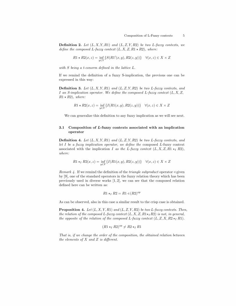
Definition 2. Let (L,X, Y,R1) and (L,Z, Y,R2) be two L-fuzzy contexts, wedefine the composed L-fuzzy context (L,X,Z,R1 ? R2), where:
R1 ? R2(x, z) = infy∈YS(R1′(x, y), R2(z, y)) ∀(x, z) ∈ X × Z
with S being a t-conorm defined in the lattice L.
If we remind the definition of a fuzzy S-implication, the previous one can beexpressed in this way:
Definition 3. Let (L,X, Y,R1) and (L,Z, Y,R2) be two L-fuzzy contexts, andI an S-implication operator. We define the composed L-fuzzy context (L,X,Z,R1 ? R2), where:
R1 ? R2(x, z) = infy∈YI(R1(x, y), R2(z, y)) ∀(x, z) ∈ X × Z
We can generalize this definition to any fuzzy implication as we will see next.
3.1 Composition of L-fuzzy contexts associated with an implicationoperator
Definition 4. Let (L,X, Y,R1) and (L,Z, Y,R2) be two L-fuzzy contexts, andlet I be a fuzzy implication operator, we define the composed L-fuzzy contextassociated with the implication I as the L-fuzzy context (L,X,Z,R1 ?I R2),where:
R1 ?I R2(x, z) = infy∈YI(R1(x, y), R2(z, y)) ∀(x, z) ∈ X × Z
Remark 4. If we remind the definition of the triangle subproduct operator / givenby [9], one of the standard operators in the fuzzy relation theory which has beenpreviously used in diverse works [1, 2], we can see that the composed relationdefined here can be written as:
R1 ?I R2 = R1 / (R2)op
As can be observed, also in this case a similar result to the crisp case is obtained.
Proposition 4. Let (L,X, Y,R1) and (L,Z, Y,R2) be two L-fuzzy contexts. Then,the relation of the composed L-fuzzy context (L,X,Z,R1?IR2) is not, in general,the opposite of the relation of the composed L-fuzzy context (L,Z,X,R2 ?I R1).
(R1 ?I R2)op 6= R2 ?I R1
That is, if we change the order of the composition, the obtained relation betweenthe elements of X and Z is different.

6 C. Alcalde et al.
Proof. Given two L-fuzzy contexts (L,X, Y,R1) and (L,Z, Y,R2), and a fuzzyimplication operator I, the relation of the composed L-fuzzy context (L,X,Z,R1 ?I R2) is:
R1 ?I R2(x, z) = infy∈YI(R1(x, y), R2(z, y)) ∀(x, z) ∈ X × Z
On the other hand, the relation of the composed L-fuzzy context (L,Z,X,R2 ?I R1) is defined as:
R2 ?I R1(z, x) = infy∈YI(R2(z, y), R1(x, y)) ∀(z, x) ∈ Z ×X
As, in general, given a fuzzy implication I(a, b) 6= I(b, a), then these relationsare not opposed. ut
Example 3. We have a company of temporary work in which we want to ana-lyze the suitability of some candidates to obtain some offered employments. Thecompany knows the requirements of knowledge to occupy each one of the posi-tions, represented by means of the L-fuzzy context (L,X, Y,R1), where the set ofobjects X is the set of employments, the attributes Y the necessary knowledge,and the relation among them appears in Table 1 with values in the chain L=0,0.1, 0.2, . . . , 1.
Table 1. The requirements of knowledge to obtain each one of the employments.
R1 computer science accounting mechanics cooking
domestic helper 0.1 0.3 0.1 1waiter 0 0.4 0 0.7
accountant 0.9 1 0 0car salesman 0.5 0.7 0.9 0
On the other hand, we have the knowledge of some candidates for thesepositions, represented by the L-fuzzy context (L,Z, Y,R2) in which the objectsare the different candidates to occupy the jobs, the attributes the necessaryknowledge and the relation among them is given by Table 2.
A candidate will be suitable to obtain a job if he owns all the knowledgerequired in this position. Therefore, to analyze what candidate is adapted foreach job, we would use the composed L-fuzzy context (L,X,Z,R1 ? R2). Therelation of this composed context, calculated using the Lukasiewicz implicationoperator, is the represented in Table 3.
To obtain the information of this L-fuzzy context we will use the ordinarytools of the L-fuzzy Concept Theory to analyze the associated L-fuzzy concepts.Thus, for example, if we want to find the best candidate to occupy the job ofwaiter, we take the set:
Composition of L-Fuzzy contexts 7
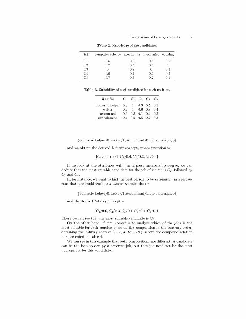
Table 2. Knowledge of the candidates.
R2 computer science accounting mechanics cooking
C1 0.5 0.8 0.3 0.6C2 0.2 0.5 0.1 1C3 0 0.2 0 0.3C4 0.9 0.4 0.1 0.5C5 0.7 0.5 0.2 0.1
Table 3. Suitability of each candidate for each position.
R1 ? R2 C1 C2 C3 C4 C5
domestic helper 0.6 1 0.3 0.5 0.1waiter 0.9 1 0.6 0.8 0.4
accountant 0.6 0.3 0.1 0.4 0.5car salesman 0.4 0.2 0.5 0.2 0.3
domestic helper/0,waiter/1, accountant/0, car salesman/0
and we obtain the derived L-fuzzy concept, whose intension is:
C1/0.9, C2/1, C3/0.6, C4/0.8, C5/0.4
If we look at the attributes with the highest membership degree, we candeduce that the most suitable candidate for the job of waiter is C2, followed byC1 and C4.
If, for instance, we want to find the best person to be accountant in a restau-rant that also could work as a waiter, we take the set
domestic helper/0,waiter/1, accountant/1, car salesman/0
and the derived L-fuzzy concept is
C1/0.6, C2/0.3, C3/0.1, C4/0.4, C5/0.4
where we can see that the most suitable candidate is C2.On the other hand, if our interest is to analyze which of the jobs is the
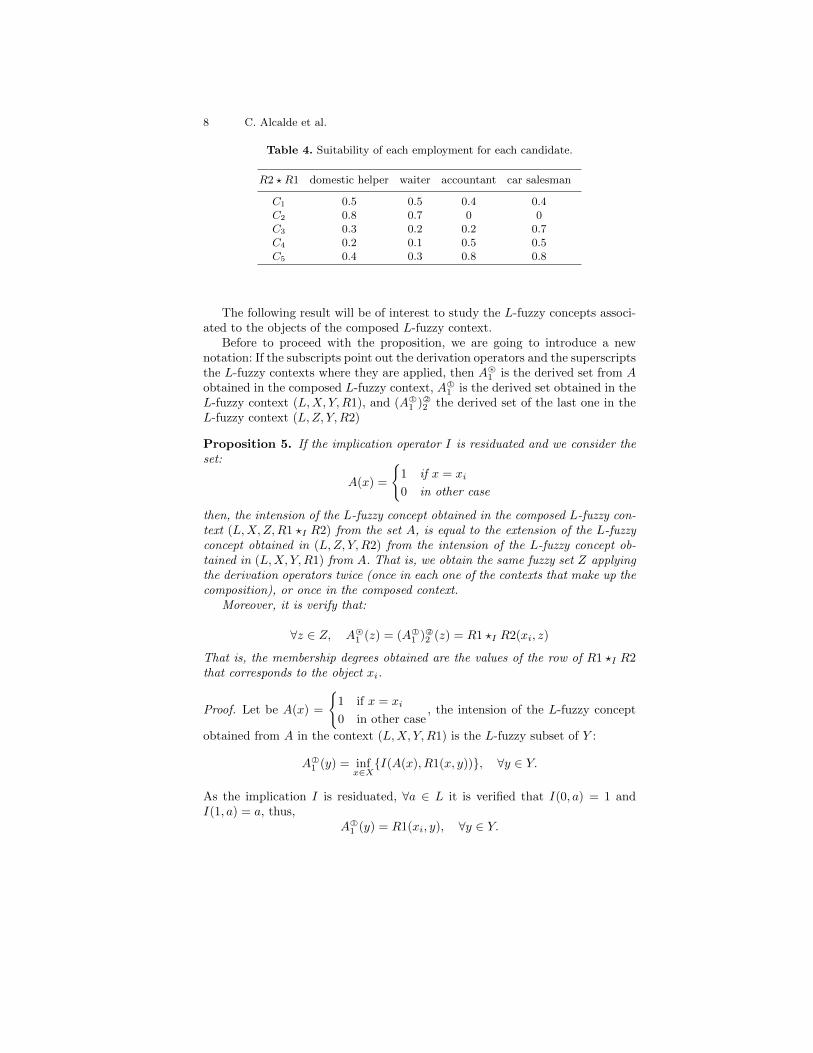
most suitable for each candidate, we do the composition in the contrary order,obtaining the L-fuzzy context (L,Z,X,R2 ? R1), where the composed relationis represented in Table 4.
We can see in this example that both compositions are different: A candidatecan be the best to occupy a concrete job, but that job need not be the mostappropriate for this candidate.
8 C. Alcalde et al.
Table 4. Suitability of each employment for each candidate.
R2 ? R1 domestic helper waiter accountant car salesman
C1 0.5 0.5 0.4 0.4C2 0.8 0.7 0 0C3 0.3 0.2 0.2 0.7C4 0.2 0.1 0.5 0.5C5 0.4 0.3 0.8 0.8
The following result will be of interest to study the L-fuzzy concepts associ-ated to the objects of the composed L-fuzzy context.
Before to proceed with the proposition, we are going to introduce a newnotation: If the subscripts point out the derivation operators and the superscriptsthe L-fuzzy contexts where they are applied, then A ?©
1 is the derived set from Aobtained in the composed L-fuzzy context, A 1©
1 is the derived set obtained in theL-fuzzy context (L,X, Y,R1), and (A 1©
1 ) 2©2 the derived set of the last one in the
L-fuzzy context (L,Z, Y,R2)
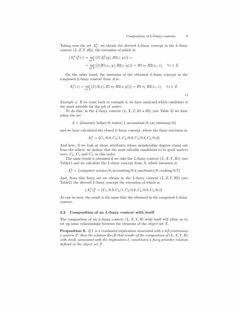
Proposition 5. If the implication operator I is residuated and we consider theset:
A(x) =
1 if x = xi
0 in other case
then, the intension of the L-fuzzy concept obtained in the composed L-fuzzy con-text (L,X,Z,R1 ?I R2) from the set A, is equal to the extension of the L-fuzzyconcept obtained in (L,Z, Y,R2) from the intension of the L-fuzzy concept ob-tained in (L,X, Y,R1) from A. That is, we obtain the same fuzzy set Z applyingthe derivation operators twice (once in each one of the contexts that make up thecomposition), or once in the composed context.
Moreover, it is verify that:
∀z ∈ Z, A ?©1 (z) = (A 1©
1 ) 2©2 (z) = R1 ?I R2(xi, z)
That is, the membership degrees obtained are the values of the row of R1 ?I R2that corresponds to the object xi.
Proof. Let be A(x) =
1 if x = xi
0 in other case, the intension of the L-fuzzy concept
obtained from A in the context (L,X, Y,R1) is the L-fuzzy subset of Y :
A 1©1 (y) = inf
x∈XI(A(x), R1(x, y)), ∀y ∈ Y.
As the implication I is residuated, ∀a ∈ L it is verified that I(0, a) = 1 andI(1, a) = a, thus,
A 1©1 (y) = R1(xi, y), ∀y ∈ Y.
Composition of L-Fuzzy contexts 9
Taking now the set A 1©1 , we obtain the derived L-fuzzy concept in the L-fuzzy
context (L,Z, Y,R2), the extension of which is:
(A 1©1 ) 2©
2 (z) = infy∈YI(A 1©
1 (y), R2(z, y)) =
= infy∈YI(R1(xi, y), R2(z, y)) = R1 ?I R2(xi, z), ∀z ∈ Z.
On the other hand, the intension of the obtained L-fuzzy concept in thecomposed L-fuzzy context from A is:
A ?©1 (z) = inf
x∈XI(A(x), R1 ?I R2(x, y)) = R1 ?I R2(xi, z), ∀z ∈ Z.
utExample 4. If we come back to example 3, we have analyzed which candidate isthe most suitable for the job of waiter.
To do this, in the L-fuzzy context (L,X,Z,R1 ? R2) (see Table 3) we havetaken the set
A = domestic helper/0,waiter/1, accountant/0, car salesman/0
and we have calculated the closed L-fuzzy concept, where the fuzzy intension is:
A ?©1 = C1/0.9, C2/1, C3/0.6, C4/0.8, C5/0.4
And here, if we look at those attributes whose membership degrees stand outfrom the others, we deduce that the most suitable candidates to be good waiterswere, C2, C1 and C4, in this order.
The same result is obtained if we take the L-fuzzy context (L,X, Y,R1) (seeTable1) and we calculate the L-fuzzy concept from A, which intension is:
A 1©1 = computer science/0, accounting/0.4,mechanics/0, cooking/0.7
And, from this fuzzy set we obtain in the L-fuzzy context (L,Z, Y,R2) (seeTable2) the derived L-fuzzy concept the extension of which is:
(A 1©1 ) 2©
2 = C1/0.9, C2/1, C3/0.6, C4/0.8, C5/0.4
As can be seen, the result is the same that the obtained in the composed L-fuzzycontext.
3.2 Composition of an L-fuzzy context with itself
The composition of an L-fuzzy context (L,X, Y,R) with itself will allow us toset up some relationships between the elements of the object set X.
Proposition 6. If I is a residuated implication associated with a left continuoust-conorm T , then the relation R?IR that results of the composition of (L,X, Y,R)with itself, associated with the implication I, constitutes a fuzzy preorder relationdefined in the object set X.

10 C. Alcalde et al.
Proof. 1. First, we prove that it is a reflexive relation, that is, the relationverifies:
∀x ∈ X, R ?I R(x, x) = 1.
By the definition of the composition associated with an implication operator,we have
∀x ∈ X, R ?I R(x, x) = infy∈YI(R(x, y), R(x, y)),
and, as any residuated implication verifies that I(a, a) = 1, ∀a ∈ L, then
∀x ∈ X, R ?I R(x, x) = 1.
2. To see that R ?I R is a T -transitive relation, we have to prove that
∀x, t, z ∈ X, T (R ?I R(x, t), R ?I R(t, z)) ≤ R ?I R(x, z),
that is, the following inequality must be verified:
T
(infα∈YI(R(x, α), R(t, α)), inf
β∈YI(R(t, β), R(z, β))
)≤
infα∈YI(R(x, α), R(z, α)).
By the monotony of the t-norm, we have:
T
(infα∈YI(R(x, α), R(t, α)), inf
β∈YI(R(t, β), R(z, β))
)≤
infα∈Y
T
(I(R(x, α), R(t, α)), inf
β∈YI(R(t, β), R(z, β))
)≤
infα∈YT (I(R(x, α), R(t, α)), I(R(t, α), R(z, α))) .
As the used t-norm T is left-continuous, we know that [7]
∀a, b, c ∈ [0, 1], T (I(a, b), I(b, c)) ≤ I(a, c),
and it is verified that:
T
(infα∈YI(R(x, α), R(t, α)), inf
β∈YI(R(t, β), R(z, β))
)≤
infα∈YI(R(x, α), R(z, α)).
ut
Remark 5. The relation R ?I R is neither symmetric nor antisymmetric andthen, is neither an equivalence nor an order relation. For instance, if we take therelation R given by the table:

Composition of L-Fuzzy contexts 11
R y1 y2 y3 y4
x1 0.1 0.3 0.5 0.1x2 0.8 0.2 0.8 0.2x3 0.4 0.7 0 0.1
then the relation R ?I R associated with the Lukasiewicz implication operatoris:
R ?I R x1 x2 x3
x1 1 0.9 0.5x2 0.3 1 0.2x3 0.5 0.5 1
and, as can be seen, is neither a symmetric nor an antisymmetric relation.
Remark 6. If we are using a non residuated implication operator, not always afuzzy preorder relation is obtained. For instance, if we take the previous relationR and we do the composition R ?I R associated with the Kleene-Dienes impli-cation (that does not verify I(x, x) = 1), then we obtain the following relation:
R ?I R x1 x2 x3
x1 0.5 0.7 0.5x2 0.2 0.2 0.2x3 0.3 0.3 0.3
that is neither a reflexive nor a fuzzy preorder relation.
The application of this composition can be very interesting in social or workrelations as we can see next:
Example 5. There are four different manufacture processes in a factory and wewant to organize the workers so that each of them is subordinate of another oneif its capacity to carry out each one of the processes of manufacture is smaller.
To model this problem, we are going to take the L-fuzzy context (L,X, Y,R),where the set of objects X is formed by the workers O1, O2, O3, O4, O5, theattributes are the different manufacture processes P1, P2, P3, P4, and the rela-tion R represents the capacity of each one of the workers to carry out each oneof the processes, in a scale of 0 to 1 (See Table 5).
The L-fuzzy context that results of the composition of this context with itselfallow us to define relations boss-subordinate between the workers so that therelation R ? R(x, y) of the compound context (associated with the Lukasiewiczimplication) gives the degree in which the worker x is subordinate of the workery. (See Table 6).

12 C. Alcalde et al.
Table 5. Capacity of the workers to carry out each one of the manufacture processes
R P1 P2 P3 P4
O1 0.7 1 0.3 0O2 0.3 0.8 0.9 0.4O3 0.1 0.2 1 0.5O4 0.5 0.3 0.2 0.4O5 1 0.5 0.8 1
Table 6. Relation ”be subordinate of”.
R ? R O1 O2 O3 O4 O5
O1 1 0.6 0.2 0.3 0.5O2 0.4 1 0.4 0.3 0.7O3 0.3 0.9 1 0.2 0.8O4 0.6 0.8 0.6 1 1O5 0 0.3 0.1 0.4 1
This will allow us, for example, to choose bosses in the group watching thecolumns of the obtained relation: In this case, we could choose as bosses of theworkers to O2 and O5 because both have as subordinate O3 and O4 and thesubordination degrees are the biggest values of the columns.
4 Conclusions and future work
This work constitutes the first approach to the problem of composition of L-fuzzy contexts. In future works we will use these results in the resolution ofother problems that seem interesting to us:
- First, this composition will be useful to study the chained L-fuzzy contexts,that is, to find relations between two defined contexts where the set of attributesof the first context is the same that the set of objects of the second one.
- On the other hand, we think that it will be useful to define the compo-sition of L-fuzzy contexts in the interval-valued case in order to study certainsituations.
Acknowledgements
This work has been partially supported by the Research Group “Intelligent Sys-tems and Energy (SI+E)” of the Basque Government, under Grant IT519-10.
References
1. C. Alcalde, A. Burusco and R. Fuentes-Gonzalez, “Analysis of certain L-Fuzzyrelational equations and the study of its solutions by means of the L-Fuzzy Concept

Composition of L-Fuzzy contexts 13
Theory.” International Journal of Uncertainty, Fuzziness and Knowledge-BasedSystems. 20 No.1 (2012), pp. 21–40.
2. E. Bartl and R. Belohlavek, “Sup-t-norm and inf-residuum are a single type ofrelational equations.” International Journal of General Systems. 40 No.6 (2011),pp. 599–609.
3. R. Belohlavek, “Fuzzy Galois connections and fuzzy concept lattices: from binaryrelations to conceptual structures”, in: Novak V., Perfileva I. (eds.): Discoveringthe World with Fuzzy Logic, Physica-Verlag (2000), pp. 462–494.
4. A. Burusco and R. Fuentes-Gonzalez, “The Study of the L-Fuzzy Concept Lattice.”Mathware and Soft Computing. 1 No.3 (1994), pp. 209–218.
5. A. Burusco and R. Fuentes-Gonzalez, “Construction of the L-Fuzzy Concept Lat-tice.” Fuzzy Sets and Systems. 97 No.1 (1998), pp. 109–114.
6. Y. Djouadi, D. Dubois and H. Prade, “On the possible meanings of degrees whenmaking formal concept analysis fuzzy.” EUROFUSE workshop. Preference Mod-elling and Decision Analysis. Pamplona, Sep 2009, pp. 253–258.
7. J. Fodor, M. Roubens. Fuzzy Preference Modelling and Multicriteria DecisionSupport. Theory and Decision Library (Kluwer Academic Publishers), Dor-drecht/Boston/London (1994).
8. A. Jaoua, F. Alvi, S. Elloumi, S. B. Yahia. “Galois Connection in Fuzzy BinaryRelations.” Applications for Discovering Association Rules and Decision Making.RelMiCS (2000), pp. 141–149.
9. L. J. Kohout, W. Bandler, Use of fuzzy relations in Knowledge representation, ac-quisition, and processing, in: L. Zadeh, J. Kacprzyk (Eds.), Fuzzy Logic for Man-agement of Uncertainty, 1992, pp. 415-435.
10. S. Krajci. “A generalized concept lattice.” Logic J. IGPL 13 (5) (2005) pp. 543–550.11. J. Medina, M. Ojeda-Aciego, and J. Ruiz-Calvino. “On multi-adjoint concept lat-
tices: definition and representation theorem.” Lect. Notes in Artificial Intelligence,4390,(2007), pp 197–209.
12. S. Pollandt, Fuzzy Begriffe: Formale Begriffsanalyse unscharfer Daten, Springer(1997).
13. R. Wille. “Restructuring lattice theory: an approach based on hierarchies of con-cepts”,in: Rival I.(ed.),Ordered Sets, Reidel, Dordrecht-Boston (1982), pp. 445–470.
14. K.E. Wolff. “Conceptual interpretation of fuzzy theory”, in: Proc. 6th EuropeanCongress on Intelligent techniques and Soft computing, 1, (1998), pp. 555–562.

Iterator-based Algorithms in Self-TuningDiscovery of Partial Implications
Jose L. Balcazar1, Diego Garcıa-Saiz2, and Javier de la Dehesa2
1 LSI Department, UPC, Campus Nord, [email protected]
2 Mathematics, Statistics and Computation Department, University of CantabriaAvda. de los Castros s/n, Santander, Spain
Abstract. We describe the internal algorithmics of our recent imple-mentation of a closure-based self-tuning associator: yacaree. This systemis designed so as not to request the user to specify any threshold. Inorder to avoid the need of a support threshold, we introduce an algo-rithm that constructs closed sets in order of decreasing support; we arenot aware of any similar previous algorithm. In order not to overwhelmthe user with large quantities of partial implications, our system filtersthe output according to a recently studied lattice-closure-based notionof confidence boost, and self-adjusts the threshold for that rule qualitymeasure as well. As a consequence, the necessary algorithmics interact incomplicated ways. In order to control this interaction, we have resortedto a well-known, powerful conceptual tool, called Iterators: this notionallows us to distribute control among the various algorithms at play ina relatively simple manner, leading to a fully operative, open-source,efficient system for discovery of partial implications in relational data.
Keywords: Association mining, parameter-free mining, iterators, Python
.
1 Introduction
The task of identifying which implications hold in a given dataset has receivedalready a great deal of attention [1]. Since [2], also the problem of identifyingpartial implications has been considered. Major impulse was received with theproposal of “mining association rules”, a very closely related concept. A majorityof existing association mining programs follow a well-established scheme [3], ac-cording to which the user provides a dataset, a support constraint, a confidenceconstraint, and, optionally, in most modern implementations, further constraintson other rule quality evaluation measures such as lift or leverage (a survey ofquality evaluation measures for partial implications is [4]). A wealth of algo-rithms, of which the most famous is apriori, have been proposed to performassociation mining.

Iterator-based Algorithms in Self-Tuning Discovery of Partial Implications 15
Besides helping the algorithm to focus on hopefully useful partial implica-tions, the support constraint has an additional role: by restricting the processto frequent (or frequent closed) itemsets, the antimonotonicity property of thesupport threshold defines a limited search space for exploration and avoids theoften too wide space of the whole powerset of items.
Instead, however, the price becomes a burden on the user, who must supplythresholds on rule evaluation measures and on support. Rule measure thresh-olds may be difficult to set correctly, but at least they offer often a “semantic”interpretation that guides the choice; for instance, confidence is (the frequentistapproximation to) the conditional probability of the consequent of the rule, giventhe antecedent, whereas lift and leverage refer to the (multiplicative or additive,respectively) deviation from independence of antecedent and consequent. Butsupport thresholds are known to be very difficult to set right. Some smallishdatasets are so dense that any exploration below 95% support, on our currenttechnology, leads to a not always graceful breakdown of the associator program,whereas other, large but sparse datasets hardly yield any association rule un-less the support is set at quantities as low as 0.1%, spanning a factor of almostone thousand; and, in order to set the “right” support threshold (whatever thatmeans), no intuitive guidance is currently known, except for the rather trivialone of trying various supports and monitoring the number of resulting rules andthe running time and memory needed.
The Weka apriori implementation automates partially the process, as follows:it explores repeatedly at several support levels, reducing the threshold from onerun to the next by a “delta” parameter (to be set as well by the user), until a givennumber of rules has been gathered. Inspired by this idea, but keeping our focus inavoiding user-set parameters, we are developing an alternative association miner.It includes an algorithm that explores closed itemsets in order of decreasingsupport. This algorithm is similar in spirit to ChARM [5], except that some ofthe accelerations of that algorithm require ordering some itemsets by increasingsupport, which becomes inapplicable in our case. Additionally, our algorithmkeeps adjusting automatically the support bound as necessary so as to be ableto proceed with the exploration within the available memory resources. Thisis, of course, more expensive in computation time, compared to a traditionalexploration with the “right” support threshold, as the number of closed frequentsets that can be filtered out right away is much smaller; on the other hand,no one can tell ahead of time which is the “right” support threshold, and ouralternative spares the user the need of guessing it. To our knowledge, this is thefirst algorithm available for mining closed sets in order of descending supportand without employing a user-fixed support threshold.
Similarly, in order to spare the user the choice of rule measure thresholds,we employ a somewhat complex (and slightly slower to evaluate) measure, theclosure-based confidence boost, for which our previous work has led to useful,implementable bounds as well as to a specific form of self-tuning [6]. It can beproved that this quantity is bounded by a related, easy to compute quantity:namely, the closure-based confidence boost is always less than or equal to the
16 Jose L. Balcazar et al.
support ratio, introduced (with a less prononceable name) in [7], and definedbelow; this bound allows us to “push” into the closure mining process a constrainton the support ratio that spares computation of rules that will fail the rulemeasure threshold. We do this by postponing the consideration of the closedsets that, upon processing, would give rise only to partial implications below theconfidence boost threshold.
As indicated, our algorithm self-tunes this threshold, which starts at a some-what selective level, by lowering it in case the output rules show it appropriate.Then, the support ratio in the closure miner is to follow suit: the constraint is tobe pushed into the closure mining process with the new value. This may meanthat previously discarded closures are to be now considered. Therefore, we mustreconcile four processes: one of mining closed frequent sets in order of decreas-ing support, filtering them according to their support ratio; two further onesthat change, along the way, respectively, the support threshold and the supportratio threshold; and the one of obtaining the rules themselves from the closeditemsets. Unfortunately, these processes interfere very heavily with each other.Closed sets are the first objects to be mined from the dataset, and are to beprocessed in order of decreasing support to obtain rules from them, but they areto be processed only if they have both high enough support, and high enoughsupport ratio. Closed sets of high support and low support ratio, however, cannotbe simply discarded: a future decrease of the self-adjusting rule measure boundmay require us to “fish” them back in, as a consequence of evaluations made“at the end” of the process upon evaluating rules; likewise, rules of low closure-based confidence boost need to be kept on hold instead of discarded, so as tobe produced if, later, they turn out to clear the threshold after adjusting it to alower level. The picture gains an additional complication from the fact that con-structing partial implications requires not only the list of frequent closures, butalso the Hasse edges that constitute the corresponding Formal Concept Lattice.
As a consequence, the varying thresholds make it difficult to organize thearchitecture of the software system in the traditional form of, first, mining thelattice of frequent closures and, then, extracting rules from them. We describehere how iterators offer a simple and efficient solution for the organization ofour partial implication miner yacaree, available at SourceForge and shown atthe demo track of a recent conference [8]. The details of the implementation aredescribed here for the first time.
2 Concepts, Notation, and Overview
In our technological context (pure Python), “generators” constitute one of theways of obtaining iterators. An iterator constructed in this way is a method (inthe object-oriented sense) containing, anywere inside, the “yield” instruction;most often, this instruction is inside some loop. This instruction acts as a “re-turn” instruction for the iterator, except that its whole status, including valuesof local variables and program counter, is stored, and put back into place at thenext call to the method. Thus, we obtain a “lazy” method that gives us, one
Iterator-based Algorithms in Self-Tuning Discovery of Partial Implications 17
by one, a sequence of values, but only computes one more value whenever it iscalled from the “consumer” that needs these values.
Generators as a comfortable way of constructing iterators are available onlyin a handful of platforms: several quite specialized lazy functional programminglanguages offer them, but, among the most common programming languages,only Python and C# include generators. Java or C++ offer a mere “iterator”interface that simply states that classes implementing iterators must offer, withspecific names, the natural operations to iterate over them, but the notion ofgenerators to program them easily is not available.
We move on to describe the essentials of our system, and the way iteratorsdefined by means of generators allow us to organize, in a clear and simple way,the various processes involved.
A given set of available items U is assumed; its subsets are called itemsets.We will denote itemsets by capital letters from the end of the alphabet, and usejuxtaposition to denote union of itemsets, as in XY . The inclusion sign as inX ⊂ Y denotes proper subset, whereas improper inclusion is denoted X ⊆ Y .For a given dataset D, consisting of n transactions, each of which is an itemsetlabeled with a unique transaction identifier, we define the support sup(X) of anitemsetX as the cardinality of the set of transactions that containX. Sometimes,the support is measured “normalized” by dividing by the dataset size; then, itis an empirical approximation to the probability of the event that the itemsetappears in a “random” transaction. Except where explicitly indicated, all ouruses of support will take the form of ratios, and, therefore, it does not matter atall whether they come absolute or normalized.
An association rule is an ordered pair of itemsets, often written X → Y .The confidence c(X → Y ) of rule X → Y is sup(XY )/sup(X). We will referoccasionally below to a popular measure of deviation from independence, oftennamed lift : assuming X ∩ Y = ∅, the lift of X → Y is
sup(XY )
sup(X) sup(Y )
where all three supports are assumed normalized (if they are not, then thedataset size must of course appear as an extra factor in the numerator).
An itemset X is called frequent if its support is greater than or equal tosome user-defined threshold: sup(X) > τ . We often assume that τ is known; nosupport bound is implemented by setting τ = 0. Our algorithms will attemptat self-tuning τ to an appropriate value without concourse of the user. Givenan itemset X ⊆ U , its closure X of X is the maximal set (with respect to setinclusion) Y ⊆ U such thatX ⊆ Y and sup(X) = sup(Y ). It is easy to see thatXis unique. An itemset X is closed if X = X. Closure operators are characterizedby the three properties of monotonicity, idempotency, and extensivity.
The support ratio was essentially employed first, to our knowledge, in [7],where, together with other similar quotients, it was introduced with the aimof providing a faster algorithm for computing representative rules. The support

18 Jose L. Balcazar et al.
ratio of an association rule X → Y is that of the itemset XY , defined as follows:
σ(X → Y ) = σ(XY ) =sup(XY )
maxsup(Z) | sup(Z) > τ, XY ⊂ Z .
For many quality measures for partial implications, including support, con-fidence, and closure-based confidence boost (to be defined momentarily), therelevant supports turn out to be the support of the antecedent and the supportof the union of antecedent and consequent. As these are captured by the corre-sponding closures, we deem inequivalent two rules X → Y and X ′ → Y ′ exactlywhen they are not “mutually redundant” with respect to the closure space de-fined by the dataset: either X 6= X ′, or XY 6= X ′Y ′. We denote that fact as(X → Y ) 6≡ (X ′ → Y ′).
We now assume sup(XY ) > τ . As indicated, our system keeps a varyingthreshold on the following rule evaluation measure: β(X → Y ) =
c(X → Y )
maxc(X ′ → Y ′) | (X → Y ) 6≡ (X ′ → Y ′), sup(X ′Y ′) > τ, X ′ ⊆ X, Y ⊆ X ′Y ′ .
This notion, known as “closure-based confidence boost”, as well as the “plainconfidence boost”, which is a simpler variant where the closure operator reducesto the identity, are studied in depth in [6]. Intuitively, this is a relative, insteadof absolute, form of confidence: we are less interested in a partial implicationhaving very similar confidence to that of a simpler one. A related formula mea-sures relative confidence with respect to logically stronger partial implications(confidence width, see [6]); the formula just given seems to work better in prac-tice. For the value of this measure to be nontrivial, XY must be a closed set;the following inequality holds:
Proposition 1. β(X → Y ) ≤ σ(X → Y ).
The threshold on β(X → Y ) is self-adjusted along the mining process, on thebasis of several properties such as coincidence with lift under certain conditions;all these details and properties are described in [6].
2.1 Architecture of yacaree
The diagram in Figure 1 shows the essentials of the class structure, for easierreference along the description of the iterators. For simplicity, a number of ad-ditional classes existing in the system are not shown. A couple of them, addedrecently, find minimal generators via standard means and implement a plainconfidence boost version appropriate for full-confidence implications; their al-gorithmics are not novel, pose no challenge, and are omitted here. We are alsoomitting discussion of classes like the Dataset class, some heap-like auxiliarydata structures, user interfaces, and a class capturing a few static values, astheir role in our description is minor or easy to understand (or both).

Iterator-based Algorithms in Self-Tuning Discovery of Partial Implications 19
Fig. 1. Partial class diagram of the associator
2.2 Class Overview
We give a brief explanation of the roles of the classes given in the diagram.Details about their main methods (the corresponding iterators) come below.
Class ItemSet keeps the information and methods to prettyprint itemsets,including information such as support; it inherits from sets all set-theoretic op-erations. Class Rule keeps both antecedent and consequent (technically, it keepsthe antecedent and the union of antecedent and consequent, as in this case thelatter is always closed, which allows for more efficient processing), and is able toprovide rule evaluation measures such as confidence or lift.
Class ClMiner runs the actual closure mining, with some auxiliary methodsto handle all details. Its main method is the iterator mine closures() (describedbelow) which yields, one by one and upon being called, all closed sets havingsupport above the threshold, in order of decreasing support. This “decreasingsupport” condition allows us to increase the support threshold, if necessary, tocontinue the exploration. As explained below, when the internal data structuresof the closure miner are about to overflow, the support threshold is increased insuch a way that half the closures found so far and still pending considerationare discarded.

20 Jose L. Balcazar et al.
Class Lattice runs its own iterator, candidate closures(), which, in turn, callsmine closures() as new closed sets become needed. Its main task is to call meth-ods that implement the algorithms from [9] and actually build the lattice ofclosed sets, so that further iterators can expect to receive closures for which theimmediate predecessors have been identified. Version 1.0 of yacaree employedthe Border algorithm but in version 1.1 we have implemented the faster al-gorithm iPred and indeed obtained around a 10% acceleration. The fact thatiPred could be employed in enumerations of closures by decreasing support wasproved in [10]. See [11] for futher discussions.
Additionally, the support ratio of each closed set is also computed here, andthe class offers yet another iterator that provides, for each closure, all the prede-cessor closures having support above a local, additional support threshold thatcan be specified at call time. In this way, we obtain all the candidate antecedentsfor a given closed set as potential consequent. This internal iterator amounts toa plain depth-first search, so that we do not discuss it further here.
Within class Lattice, two heap-structured lists keep, respectively, the closuresthat are ready to be passed on as they clear both the support and the supportratio thresholds (Lattice.ready) and the closures that clear the support thresholdbut fail the support ratio threshold (Lattice.freezer); these will be recovered incase a decrease of the confidence boost bound is to affect the support ratiopruning.
Finally, class RuleMiner is in charge of offering the system an iterator over allthe association rules passing the current thresholds of support and closure-basedconfidence boost: mine rules(). Its usage allows one to include easily furtherchecks of confidence, lift, or any other such quantity.
3 Details
This section provides details of the main iterators and their combined use toattain our goals.
3.1 ClMiner.mine closures()
The closure miner is the iterator that supports the whole scheme; it follows a“best-first” strategy, where here “best” means “highest support”. We maintain aheap containing closures already generated, but which have not been expandedyet to generate further closures after them. The heap can provide the one ofhighest support in logarithmic time, as this is the closure that comes next. Then,as this closure is passed on to the lattice constructor, items (rather, closures ofsingletons) are added to it in all possible ways, and closure operations are appliedin order to generate its closed successors, which are added to the heap unlessthey were already in it. The decreasing support condition ensures that they werenever visited before. For simplicity, we omit discussing the particular case of theempty set, which, if closed, is to be traversed first, separately.
1: identify closures of singletons

Iterator-based Algorithms in Self-Tuning Discovery of Partial Implications 21
2: organize them into a maxheap according to support3: while heap nonempty do4: consider increasing the support threshold by monitoring the available
memory5: if the support threshold must be raised then6: kill from the heap pending closures of support below new threshold,
which is chosen so that the size of the heap halves7: end if8: pop from heap the max-support itemset9: yield it
10: try to extend it with all singleton closures11: for such extensions with sufficient support do12: if their closure is new then13: add it to the heap14: end if15: end for16: end while
In order to clarify how this algorithm works, we develop the following ex-ample. Consider a dataset with 24 transactions over universe U = a, b, c, d, eof 5 items: abcde, bcde × 2, abe, cde, be, ae × 3, ab × 4, cd × 6, b × 2, a × 3. Forthis dataset, there are 12 closed sets, which we enumerate here with their cor-responding supports: ∅/24, a/12, b/11, cd/10, e/9, ab/6, ae/5, be/5, cde/4, bcde/3,abe/2, abcde/1. The empty set is treated first, separately, as indicated. Then, thefour next closures correspond to closures of singletons (the closures of c and dcoincide) and form an initial heap, containing: [a/12, b/11, cd/10, e/9].
The heap provides a as next closure in descending support; it is passedon to further processing at the “yield” instruction, and it is expanded withsingleton closures in all possible ways, enlarging the heap into containing sixpending closures: [b/11, cd/10, e/9, ab/6, ae/5, abcde/1]: each of the new sets in theheap is obtained by adding to a the closure of a singleton, and closing theresult. The next closure is b, which goes into the “yield” instruction and, subse-quently, generates two further closures to be added to the heap, which becomes:[cd/10, e/9, ab/6, ae/5, be/5, bcde/3, abcde/1]. The closure ab generated from b isomitted, as it is repeated since it was already generated from a.
For illustration purposes, we assume now that the length of the heap, cur-rently 7, is deemed too large. Of course, in a toy example like this one there isno need of moving up the support threshold, but let’s do it anyway: assume thatthe test indicates that the heap is occupying too much memory, incurring in arisk of soon-coming overflow. Then, the support is raised as much as necessaryso as to halve the length of the heap. Pending closures of support 5 or less wouldbe discarded from the heap, the support threshold would be set at 6, and onlythree closures would remain in the heap: [cd/10, e/9, ab/6]. Each of them would beprocessed in turn, given onwards by the “yield” instruction, and expanded withall closures of singletons; in all cases, we will find that expanding any of themwith a singleton closure leads to a closure of support below 6, which is therefore

22 Jose L. Balcazar et al.
omitted as it does not clear the threshold. Eventually, these three closures in theheap are passed on, and the iterator will have traversed all closures of support6 or higher.
As a different run, assume now that we accept the growth of the heap, so thatit is not reduced. The traversal of closures would go on yielding cd, which wouldadd cde to the heap; adding either a or b to cd leads to abcde which is already inthe heap. The next closure e adds nothing new to the heap, and the next is abwhich adds abe; at this point the heap is [ae/5, be/5, cde/4, bcde/3, abe/2, abcde/1].All further extensions only lead to repeated closures, hence nothing is furtheradded to the heap, and, as it is emptied, the traversal of all the closures iscompleted.
The main property that has to be argued here is the following:
Proposition 2. As the support threshold rises, all the closed sets delivered sofar by the iterator to the next phase are still correct, that is, have support at leastthe new value of the threshold.
Proof. We prove this statement by arguing the following invariants: first, thenew threshold is bounded above by the highest support of a closure in the heap;second, all the closed sets provided so far up to any “yield” statement have sup-port bounded below by all the supports currently in the heap. These invariantsare maintained as we extract the closure C of maximum support in the heap,and also when we add to it extensions of C: indeed, C having been freshly takenoff the heap, all previous deliveries have at least the same support, whereas allextensions that are to enter the heap are closed supersets of C and must havelower support, because C is closed.
Hence, all previous deliveries have support higher than the maximum supportin the heap, which, in turn, is also higher than the new threshold; transitivitynow proves the statement.
3.2 Lattice.candidate closures()
In order to actually mine rules from the closures traversed by the loop describedin the previous section, further information is necessary: data structures to allowfor traversing predecessors, namely, the Hasse edges, that is, the immediate,nontransitive neighbors of each closure. These come from a second iterator thatimplements the iPred algorithm [9].
Additionally, we wish to push into the closure mining the confidence boostconstraint. The way to do it is to compute the support ratio of each closure, andonly pass it on to mine rules from it if this support ratio is above the confidenceboost threshold; indeed, Proposition 1 tells us that, if the support ratio is belowthe threshold, the confidence boost will be too.
Due to the condition of decreasing support, we know that the closed supersetthat defines the support ratio is exactly the first successor to appear from theclosure mining iterator. As soon as one successor of C appears, if the supportratio is high enough, we can yield C, as the Hasse edges to its own predecessors

Iterator-based Algorithms in Self-Tuning Discovery of Partial Implications 23
are guaranteed to have been set before. If the support ratio is not enough, it iskept on a “freezer” (again a heap-like structure) from where it might be “fishedback in” if the confidence boost threshold decreases later on.
One has to be careful that the same closed set, say C, may be the firstsuccessor of more than one predecessor. As we set the predecessors C ′ of C, wemove to the “ready” heap those that have C as first successor, if their supportratio is high enough; then we yield them all. Additionally, as we shall see, it mayhappen that RuleMiner.mine rules() moves closures from “freezer” to “ready”.We explain this below.
1: for each closed set C yielded by ClMiner.mine closures() do2: apply a Hasse edges algorithm (namely iPred) to set up the lattice edges
connecting C to its predecessors3: for each unprocessed predecessor C ′ do4: compute the support ratio of C ′
5: if support ratio is over the rule evaluation threshold then6: add C ′ to the “ready” heap7: else8: add C ′ to the “freezer” heap9: end if
10: end for11: for each closure in the “ready” heap do12: yield it13: end for14: end for
We observe here that we are not guaranteeing decreasing support order in thisiterator, as the changes to the support ratio threshold may swap closures withrespect to the order in which they were obtained. What we do need is that themost basic iterator, ClMiner.mine closures(), does provide them in decreasingsupport order, first, to ensure that the support threshold can be raised if nec-essary, and, second, to make sure that the support ratio is correctly computedfrom the first successor found for each closure.
Along the same example as before, consider, for instance, what happens whenClMiner.mine closures() yields the closure ab to Lattice.candidate closures().The iPred algorithm identifies a and b as immediate predecessors of ab, andthe corresponding Hasse edges are stored. Then, both a and b are identified asclosures whose first successor (in decreasing support) has just appeared; indeed,other successors have less support than ab. The support ratios of a and b, namely,12/6 = 2 and 11/6, are seen to be higher than the confidence boost threshold(which starts at 1.15 by default) and both a and b are moved to the “ready”heap and yielded to the subsequent rule mining phase. On the other hand, if theconfidence boost threshold was, say, at 1.4, upon processing bcde we would find4/3 < 1.4 as support ratio of cde, and this closure would wait in the freezer heap,until (if at all) a revised lower value of the confidence boost threshold would letit through, by moving it from the freezer queue to the ready queue.

24 Jose L. Balcazar et al.
3.3 RuleMiner.mine rules()
In the class RuleMiner, which inherits from Lattice, the iterator mine rules()relies on the closures provided by the previous iterator in the pipeline:
1: reserved rules = [ ]2: for each closure from candidate closures() do3: for each predecessor having high enough support so as to reach the con-
fidence threshold do4: form a rule r with the predecessor as antecedent and the closure as
consequent5: use it to revise the closure-based confidence boost threshold6: if threshold decreased then7: move from Lattice.freezer to Lattice.ready those closures whose sup-
port ratio now passes the new threshold8: for each rule in reserved rules do9: if its closure-based confidence boost threshold passes the threshold
then10: yield it11: else12: keep it in reserved rules13: end if14: end for15: end if16: if the closure-based confidence boost of r passes the threshold then17: yield r18: else19: keep it in reserved rules20: end if21: end for22: end for
Each closure makes available an iterator over its predecessors in the closureslattice (closed proper subsets), up to a given support level that we can specifyupon calling it. For instance, at the closure bcde, of support 3, and assuminga confidence threshold of 0.6, we would explore predecessors be and cde, whichlead to rules be → cd and cde → b. The confidence boost has to be checked,but part of the task is already made since the very fact that the closure bcdearrived here implies that its support ratio is over the confidence boost threshold.In this case, the support ratio of closure bcde is 3. We must test confidences withsmaller antecedents (see [6]). As the confidences of b → cd and e → cd are lowenough, the rule be → cd becomes indeed reported; cde → b does as well, afterchecking how low the confidences of cd→ b and e→ b are.
The revision of the closure-based confidence boost threshold can be donein a number of ways. The current implementation keeps computing the lift ofthose rules whose antecedent is a singleton, as the condition on support ratioensures that, in this case, it will coincide with the confidence boost [6]; these liftvalues enter a weighted average with the current threshold, and, if the average is

Iterator-based Algorithms in Self-Tuning Discovery of Partial Implications 25
sufficiently smaller, the threshold is decreased. Only a partial justification existsso far for this choice.
When the threshold for confidence boost decreases, closures whose supportratio was too low may become now high enough; thus, the freezer is explored andclosures whose support ratio is now above the new confidence boost thresholdare moved into the ready queue (lines 6 and 7), to be processed subsequently.
3.4 System
The main program simply traverses all rules, as obtained from the iteratormine rules(), in the class RuleMiner:
1: for each rule in RuleMiner.mine rules() do2: account for it3: end for
What is to be done with each rule depends on the instructions from the userinterface, but usually we count how many of them are obtained and we writethem all on disk, maybe up to a fixed limit on the number of rules (that canbe modified by editing the source code). In this case, we report those of highestclosure-based confidence boost.
4 A Second Implementation
With a view to offering this system in a more widespread manner, we have de-veloped a joint project with KNIME GmbH, a small company that develops theopen source data mining suite KNIME. This data mining suite is implementedin Java. Hence, we have constructed a second implementation in Java.
However, the issue is not fully trivial because of two main reasons. The firstis that the notion of iterator in Java is different from that in Python, and is notobtained from generators: the “yield” instruction, which saves the state of aniteration at the time it is invoked, does not exist in Java, which simply declaresthat hasNext() and next() methods must be made available: respectively, toknow whether there are more elements to process and to get the next element.A second significative change is that the memory control to ensure that the listof pending closures does not overflow has to be made in terms of the memorymanagement API of KNIME, and requires one extra loop to check whether thedecrease in memory usage was sufficient.
Therefore, we have to use the Iterator class to “copy”, to the extent possible,the “yield” behavior, saving all necessary information to continue in queues andlists. The three most affected methods for this issue are, of course, mine rules(),candidate closures() and mine closures(). We describe here only mine rules().
In this case, a queue, called ready rules, is needed in order to store therules that are built from the current closure among the candidates and haveachieved the support, confidence, and confidence boost requirements. Rules thatdo not clear these thresholds are stored in another queue, reserved rules, as inthe Python implementation. The code is shown next:

26 Jose L. Balcazar et al.
1: reserved rules = empty queue of rules2: ready rules = empty queue of rules3: ready rules iterator = iterator for ready rules4: while !ready rules iterator.hasNext() do5: for each closure from candidate closures() do6: for each predecessor having high enough support so as to reach the
confidence threshold do7: form a rule r with the predecessor as antecedent and the closure as
consequent8: use it to revise the threshold for the rule evaluation measure9: if threshold decreased then
10: move from Lattice.freezer to Lattice.ready those closures whosesupport ratio now passes the new threshold
11: for each rule in reserved rules do12: if its rule measure passes the new threshold then13: store it in ready rules14: else15: keep it in reserved rules16: end if17: end for18: end if19: if the rule measure of r passes the threshold then20: store it in ready rules21: else22: keep it in reserved rules23: end if24: end for25: end for26: end while27: return ready rules
In Lattices.candidate closures(), the candidate closures are likewise stored ina list called cadidate closures list in order that mine rules method can obtainthem. The program is constructed in the same way as the one just described,and is omitted here.
The last method that needs a change in the translation from Python to Javaand KNIME is clminer.mine closures(), and it consists of storing in a list calledmax-support itemset list the candidate itemsets that obey the max-support re-quirement, and of returning this list at the end of the method. In this caseiterators aren’t needed beacuse in this method is only required to store andreturn the list, so next() and hastNext() methods are not used.
1: max-support itemset list = empty list of itemset2: identify closures of singletons3: organize them into a maxheap according to support4: while heap nonempty do
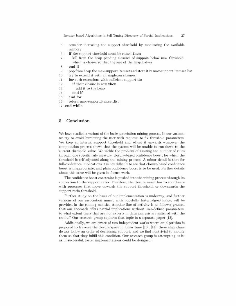
Iterator-based Algorithms in Self-Tuning Discovery of Partial Implications 27
5: consider increasing the support threshold by monitoring the availablememory
6: if the support threshold must be raised then7: kill from the heap pending closures of support below new threshold,
which is chosen so that the size of the heap halves8: end if9: pop from heap the max-support itemset and store it in max-support itemset list
10: try to extend it with all singleton closures11: for such extensions with sufficient support do12: if their closure is new then13: add it to the heap14: end if15: end for16: return max-support itemset list17: end while
5 Conclusion
We have studied a variant of the basic association mining process. In our variant,we try to avoid burdening the user with requests to fix threshold parameters.We keep an internal support threshold and adjust it upwards whenever thecomputation process shows that the system will be unable to run down to thecurrent threshold value. We tackle the problem of limiting the number of rulesthrough one specific rule measure, closure-based confidence boost, for which thethreshold is self-adjusted along the mining process. A minor detail is that forfull-confidence implications it is not difficult to see that closure-based confidenceboost is inappropriate, and plain confidence boost is to be used. Further detailsabout this issue will be given in future work.
The confidence boost constraint is pushed into the mining process through itsconnection to the support ratio. Therefore, the closure miner has to coordinatewith processes that move upwards the support threshold, or downwards thesupport ratio threshold.
Further study on the basis of our implementation is underway, and furtherversions of our association miner, with hopefully faster algorithmics, will beprovided in the coming months. Another line of activity is as follows: grantedthat our approach offers partial implications without user-defined parameters,to what extent users that are not experts in data analysis are satisfied with theresults? Our research group explores that topic in a separate paper [12].
Additionally, we are aware of two independent works where an algorithm isproposed to traverse the closure space in linear time [13], [14]; these algorithmsdo not follow an order of decreasing support, and we find nontrivial to modifythem so that they fulfill this condition. Our research group is attempting at it,as, if successful, faster implementations could be designed.

28 Jose L. Balcazar et al.
References
1. Ganter, B., Wille, R.: Formal Concept Analysis: Mathematical Foundations.Springer-Verlag (1999)
2. Luxenburger, M.: Implications partielles dans un contexte. Mathematiques etSciences Humaines 29 (1991) 35–55
3. Agrawal, R., Mannila, H., Srikant, R., Toivonen, H., Verkamo, A.I.: Fast discov-ery of association rules. In: Advances in Knowledge Discovery and Data Mining.AAAI/MIT Press (1996) 307–328
4. Geng, L., Hamilton, H.J.: Interestingness measures for data mining: A survey.ACM Comput. Surv. 38(3) (2006)
5. Zaki, M.J., Hsiao, C.J.: Efficient algorithms for mining closed itemsets and theirlattice structure. IEEE Transactions on Knowledge and Data Engineering 17(4)(2005) 462–478
6. Balcazar, J.L.: Formal and computational properties of the confidence boost inassociation rules. Available at: [http://personales.unican.es/balcazarjl]. Extendedabstract appeared as ”Objective novelty of association rules: Measuring the confi-dence boost. In Yahia, S.B., Petit, J.M., eds.: EGC. Volume RNTI-E-19 of Revuedes Nouvelles Technologies de lInformation., Cepadu‘es-Editions (2010) 297-302”(2010)
7. Kryszkiewicz, M.: Closed set based discovery of representative association rules. InHoffmann, F., Hand, D.J., Adams, N.M., Fisher, D.H., Guimaraes, G., eds.: Proc.of the 4th International Symposium on Intelligent Data Analysis (IDA). Volume2189 of Lecture Notes in Computer Science., Springer-Verlag (2001) 350–359
8. Balcazar, J.L.: Parameter-free association rule mining with yacaree. In Khenchaf,A., Poncelet, P., eds.: EGC. Volume RNTI-E-20 of Revue des Nouvelles Technolo-gies de l’Information., Hermann-Editions (2011) 251–254
9. Baixeries, J., Szathmary, L., Valtchev, P., Godin, R.: Yet a faster algorithm forbuilding the Hasse diagram of a concept lattice. In Ferre, S., Rudolph, S., eds.:Proc. of the 7th International Conference on Formal Concept Analysis (ICFCA).Volume 5548 of Lecture Notes in Artificial Intelligence., Springer-Verlag (2009)162–177
10. Balcazar, J.L., Tırnauca, C.: Border algorithms for computing Hasse diagramsof arbitrary lattices. In Valtchev, P., Jaschke, R., eds.: ICFCA. Volume 6628 ofLecture Notes in Computer Science., Springer (2011) 49–64
11. Kuznetsov, S.O., Obiedkov, S.A.: Algorithms for the construction of concept lat-tices and their diagram graphs. In Raedt, L.D., Siebes, A., eds.: Proc. of the5th European Conference on Principles of Data Mining and Knowledge Discovery(PKDD). Volume 2168 of Lecture Notes in Artificial Intelligence., Springer-Verlag(2001) 289–300
12. Garcıa-Saiz, D., Zorrilla, M., Balcazar, J.L.: Closures and partial implications ineducational data mining. ICFCA, Supplementary proceedings (2012)
13. Ganter, B.: Two basic algorithms in concept analysis (preprint 1987). In Kwuida,L., Sertkaya, B., eds.: ICFCA. Volume 5986 of Lecture Notes in Computer Science.,Springer (2010) 312–340
14. Uno, T., Asai, T., Uchida, Y., Arimura, H.: An efficient algorithm for enumeratingclosed patterns in transaction databases. In Suzuki, E., Arikawa, S., eds.: DiscoveryScience. Volume 3245 of Lecture Notes in Computer Science., Springer (2004) 16–31

Completing Terminological Axioms with FormalConcept Analysis
Alexandre Bazin and Jean-Gabriel Ganascia
Universite Pierre et Marie Curie, Laboratoire d’Informatique de Paris 6Paris, France
Abstract. Description logics are a family of logic-based formalisms usedto represent knowledge and reason on it. That knowledge, under theform of concepts and relationships between them called terminologicalaxioms, is usually manually entered and used to describe objects in agiven domain. That operation being tiresome, we would like to automat-ically learn those relationships from the set of instances using dataminingtechniques. In this paper, we study association rules mining in the de-scription logic EL. First, we characterize the set of all possible conceptsin a given EL language. Second, we use those characteristics to developan algorithm using formal concept analysis to mine the rules more effi-ciently.
Keywords: Description Logic, Association Rules Mining, Ontology
1 Introduction
Ontologies are knowledge representation tools used in various domains of appli-cation. The semantic web, for example, makes an extensive use of them. Theyare essentially composed of a list of concepts relevant to a particular domainand relations (mainly inclusion and equivalence, i.e. hierarchical relations) ex-isting between them. Description Logics (DL) are increasingly popular logicalframeworks used to represent ontologies and on which is based the OWL1 lan-guage for the semantic Web. They have a great representation power and allowpowerful reasoning tools. However, the construction of ontologies, usually per-formed manually by knowledge engineers, is both a tedious and tricky operation.One of the difficulties is to ensure the consistency and the completeness of theset of relations between concepts. in order to facilitate this step, we propose toautomatize, at least partially, the process of relation generation.
Based on the lattice theory, Formal Concept Analysis (FCA) is a mathemat-ical framework that also deals with concepts and their hierarchical relationships.FCA provides solid theoretical foundations for association rule learning tools.
1 OWL is an acronym for Ontology Web Language, which is a W3C standard
30 A. Bazin et al.
It therefore seems to be a good natural candidate for this task, i.e. for the au-tomatic generation of relationships between concepts, from object descriptions,i.e. from concept instances.
Despite differences between the use of the notion of concept in these twoformalisms, it would be interesting to combine them both and draw benefitsfrom their mutual advantages. This combination has already been investigatedand two main approaches exist. The first integrates operators of FCA to theDL framework in order to be able to apply learning algorithms directly to aknowledge base expressed in DL [4] [8], the second, which corresponds to ourpresent work, translates data from DL to a form comprehensible by FCA, inother words, it interprets DL formalism within the lattice theory [2] [3] [7].
We claim that, by using the specific lattice structure of the set of conceptsof description logics, we will be able to modify classical FCA algorithms inorder to build complete and consistent sets of terminological axioms from objectdescriptions given as assertions. This work, which constitutes a first attempt inthis direction, will make use of a simple description logic, which is EL. But, theapproach is not restricted to EL; it will certainly be possible to generalize it toother DL, which will be investigated in further work.
Apart from the introduction and the conclusion, this paper is divided intofour parts. The first briefly recalls the usual definitions in both DescriptionLogics and Formal Concept Analysis, the second characterizes the structure ofthe set of EL-concepts making use of the function Φ that is the set of subsetsof incomparable elements of a language, the third describes a simple associationrule learning algorithm that works within the set of EL-concepts previouslydescribed. It then studies the properties of the set of terminological axioms thatit generates. The last part is dedicated to a brief example, which illustrates thedifferent notions presented in this paper.
2 Definitions and Recalls
2.1 Description Logics
Descriptions logics are decidable fragments of first-order logic used to representand reason on knowledge. Syntactically, every description logic language makesuse of a set of concept namesNC , a set of role namesNR and a set of object namesNO and combines them using constructors to build concept descriptions or, inshort, concepts. The set of constructors used defines the language’s expressionpower and the complexity of its reasoning procedures. In this paper, we willconsider the logic EL. In it, every concept name is a concept description and, forany concept descriptions A and B and any role r, AuB and ∃r.A are also conceptdescriptions. Having only two constructors, this logic is one of the simplest.
Semantics are defined by means of interpretations. An interpretation is a pairI = (∆I , .I) where ∆I is a set of objects called the domain and .I a functionmapping every concept name C to a subset CI of ∆I and every role name r
Completing Terminological Axioms with Formal Concept Analysis 31
to a binary relation rI ⊆ ∆I ×∆I . As such, concepts are defined by the set ofobjects which belong to them.
An important notion in description logic systems is the subsumption relationbetween concept descriptions. Given two concept descriptions C and D, we saythat D subsumes C (C v D) if the set of objects belonging to C is included inthe set of objects belonging to D (CI ⊆ DI) for all interpretations I. For a givenTBox T , we say that D subsumes C with respect to T (C vT D) if CI ⊆ DI
for every model of T . If C v D and D v C, it gives the definition C ≡ D.Constructions such as C v D and C ≡ D expressing subsumption relations arecalled terminological axioms.
For any given concept C, role r and object names o and o′, o : C and (o, o′) : rare called assertional sentences. The constructions o : C means that the objecto belongs to the concept C and (o, o′) : r means that the object o′ fulfills therole r for the object o.
A knowledge base consists of a TBox and an ABox. The TBox is constitutedof terminological axioms, which we try to learn in this paper, and concept defi-nitions. The ABox is a set of assertional sentences and can be viewed as a set ofdescriptions of objects.
2.2 Formal Concept Analysis
In formal concept analysis (FCA), we call formal context a triplet (O,A,R)where O is a set of objects, A a set of attributes and R a binary relation betweenobjects and attributes. We say here that (o, a) ∈ R means that a describes o.
We have at our disposal two functions .′ such as
.′ : 2A 7→ 2O
A′ =⋂
a∈Ao ∈ O | (o, a) ∈ R (1)
and
.′ : 2O 7→ 2A
O′ =⋂
o∈Oa ∈ A | (o, a) ∈ R (2)
A′ is then the set of objects described by every attribute of A and O′ is theset of attributes describing every object of O. If A ⊆ B, then B′ ⊆ A′ and ifO ⊆ P then P ′ ⊆ O′. As such, those two functions form a Galois Connection.
A formal concept is defined as a pair (E, I) ∈ AO × 2A where E = I ′
and I = E′. We say that E and I are closed. E and I are respectively calledthe extent and the intent of the concept. In order to prevent confusion, formal

32 A. Bazin et al.
concept will not be abbreviated and the term concept will be used exclusivelyfor DL-concepts.
We call FC(O,A,R) the set of formal concepts we can find in (O,A,R).We can define an order < (a relation “is more general than”) on this set suchas (E, I) < (F, J) ⇔ (F ⊂ E and I ⊂ J) and the pair (FC(O,A,R), <)satisfies the properties of a complete lattice. Such a lattice is called a concept(or Galois) lattice. For example, for a formal context in which O = a, b, c, d, e,A = 1, 2, 3, 4, 5 and R = (a, 2), (a, 4), (b, 3), (b, 5), (c, 1), (c, 2), (c, 4), (d, 2),(d, 3), (e, 2), (e, 4) we obtain the following concept lattice.
(,1,2,3,4,5)
(c,1,2,4) (b,3,5) (d,2,3)
(a,c,e,2,4) (b,d,3)
(a,b,c,d,e,)
Fig. 1. A Concept Lattice
FCA allows us to find implications in the formal context which are orderedpairs (B,C), often written B → C. An implication B → C holds in a context ifevery object described by every attribute in B is also described by every attributein C.
Definition 1. We say that a set X ∈ A respects an implication B → C ifB ⊆ X implies C ⊆ X.
An implication B → C follows from a set of implications L if every X ∈ Athat respects every implication in L respects B → C. A set L of implicationsis then called a basis if every implication in L holds in the context and everyimplication that holds in the context follows from L.
It is a known fact that X → X ′′ | X ⊆ A is an implicational basis whichmeans that, in order to obtain a basis of minimal cardinality, we need only tofind implications whose right-hand side are concept intents. Finding suitableleft-hand side has thus been the subject of many works.
Definition 2. A set X ∈ A is a pseudo-intent of the context (O,A,R) if X isnot a concept intent and, for all pseudo-intent Y ⊂ X, Y ′′ ⊆ X.

Completing Terminological Axioms with Formal Concept Analysis 33
Definition 3. The set of implications X → X ′′ | X is a pseudo-intent iscalled a Duquenne-Guigues Basis.
The Duquenne-Guigues Basis is the minimal set of implication from whichwe can find every other implications that hold through inference.
3 The Set of Concept Descriptions
Before using an association rules learning algorithm, we will study the structureof the set of concepts one can build with the description logic EL.
We will use Ω to denote the set of terminological axioms A v B in an acyclicTBox T . NC = AC ∪DC will denote the set of concept names used in T withAC the set of atomic concepts and DC the set of defined concepts, appearing inthe left hand side of definitions. The set of pairs (C1, C2) such as C1 ≡ C2 willbe called Def(T ). Ω induces a partial order on the set of equivalence classes ofconcepts, noted NC≡ , used in axioms (if (x u y v z) ∈ Ω, we will consider thereis some d in DC such as d ≡ x u y). We will simply use b ≤ a for [a]≡ v [b]≡.(NC≡ ,≤) is then a partially ordered set such as, for all x in NC , [>]≡ ≤ [x]≡.For clarity purposes, we will now use CN0 to denote a set of concept namescontaining a unique representative of each equivalence class together with theorder ≤. Obviously, CN0 is isomorphic to (NC≡ ,≤).
We are interested in the set of every possible concept we can construct withNC , NR and the constructors u and ∃. Suppose there are two concepts A andB such as A v B. This means that AI ⊆ BI so A uB ≡ A. Those two conceptdescriptions being equivalent we consider they are the same and we do not wantto include both of them in the set of possible concepts. As such, we want the setof concepts resulting from the conjunction of incomparable elements.
Definition 4. We call Φ(CN0) = X ⊆ CN0 | x ∈ X ∧ y ∈ X ⇒ x||y the setof subsets of incomparable elements of CN0
We call Φ(CN0) the set of subsets of incomparable elements of CN0 anduA the concept built from the conjunction of the elements of A. For any twoelements C,D ∈ Φ(CN0), we say that C ≤ D if and only if uD v uC. Thatis, C ≤ D if and only if for every element c ∈ C there is some d ∈ D suchas c ≤ d. Evidently, Φ(CN0) is isomorphic to the set of ideals of CN0 orderedby inclusion and its elements are the sets of maximal elements of those ideals.Φ(CN0) is then a distributive lattice.
Proposition 1. For any two elements A,B ∈ Φ(CN0), A ∧ B = Max(x ∈CN0 | ∃a ∈ A, ∃b ∈ B, x ≤ a & x ≤ b) and A ∨B = Max(A ∪B).
u(A ∧ B) corresponds to the least common subsumer of uA and uB andu(A ∨ B) to the most specific concept subsumed by uA and uB. They can beeasily computed from CN0.
Φ(CN0) being finite and distributive, for all A and B in Φ(CN0), there is aleast element X such as A∨X ≥ B called difference and noted B \A. It is equal

34 A. Bazin et al.
to Max(↓ B\ ↓ A) where ↓ A is the set of elements lower or equal to elementsof A in CN0.
Proposition 2. For a given linear extension σ of CN0, the relation A B ⇔B \A = Maxσ(B) defines a spanning tree of the covering graph of Φ(CN0).
The spanning tree gives us, for every element A ∈ Φ(CN0), a unique pathfrom > to A in which A B ⇒ A ≤ B.
Φ(CN0) is the set of different conjunctions of concept names based on thesubsumption relation. However, the TBox can also contain equivalences betweenelements of Φ(CN0). If (A,B u C) ∈ Def(T ) then B ≤ A and C ≤ A inCN0. In Φ(CN0), A is thus strictly greater than B,C. Those two conceptsbeing equivalent, every element greater or equal to B,C and lower than Ais considered redundant.
Definition 5. Φ(CN0)Def(T ) = Φ(CN0) \ B | (A,B) ∈ Def(T ) is the set ofsubsets of incomparable elements of CN0 without the elements corresponding toright-hand sides of definitions of Φ(C,≤X)Def(T ) the TBox.
Proposition 3. For any two elements A,B ∈ Φ(CN0)Def(T ), A ∧B inΦ(CN0)Def(T ) is equal to A ∧B in Φ(CN0).
Proposition 4. For all A and B in Φ(CN0)Def(T ), the difference A \ B inΦ(CN0) is an element of Φ(CN0)Def(T ).
These operations on Φ(CN0)Def(T ) are thus the same than on Φ(CN0). Thedifferences appear when we try to compute the upper cover of an element D, i.e.elements immediately greater than D. We call Cand – for candidate – the set ofminimal elements not lower than elements of D in CN0. In Φ(CN0), the uppercover of D is then Max(D∪ c) | c ∈ Cand. In Φ(CN0)Def(T ), if there is some(L,R) ∈ Def(T ) such as L ≥ Max(D ∪ c) ≥ R, c must be removed from thelist of candidates and L added if it is minimal in Cand \ c. In order to find theelements following D in the spanning tree of Φ(CN0)Def(T ) induced by some σit would then be sufficient to remove the candidates c such as c ≤σ d for some din D. The algorithm is as follows :
Algorithm 1
Require: CNn, D1: Cand = c ∈ CNn | c ∈Min(CN0\ ↓ D) and ∀d ∈ D, c ≥σ d2: for each c ∈ Cand do3: if ∃(L,R) ∈ Def(T ) such as L ≥Max(D ∪ c) ≥ R then4: Cand = Min((Cand \ c) ∪ L)5: end if6: end for7: Return Max(D ∪ c) | c ∈ Cand

Completing Terminological Axioms with Formal Concept Analysis 35
Now, Φ(CN0)Def(T ) is only the lattice of concepts built from a conjunctionof concept name without roles. However, it gives us informations on the struc-ture of the set of role-concepts. We know that, for a given role r, A v B ⇒∃r.A v ∃r.B. The partially ordered set of roles of a depth 1 is then isomorphic
to Φ(CN0)Def(T ). We use CN1r to denote it. If CN1 = CN0
⋃|NR|i=1 CN1
ri is theset of both concept names and roles of depth 1 together with the partial orderinduced by Ω, then Φ(CN1)Def(T ) is the lattice of concepts containing roles
up to a depth 1. Recursively, Φ(CNn)Def(T ) where CNn = CN0⋃|NR|i=1 CNn
riwith CNn
ri isomorphic to Φ(CNn−1)Def(T ) is the set of every possible conceptdescriptions up to an arbitrary role depth n.
4 Learning Axioms with Formal Concept Analysis
As we said previously, we take the approach of creating a formal context corre-sponding to the DL-objects we want to manipulate. More precisely, we use theformal context (O,A,R) where O is a set of objects, A = Φ(CNn)Def(T ) is theset of every possible concept descriptions defined in Section 2.2 and R ⊆ O×Ais the relation associating objects to the most specific concept to which theybelong. In that respect, it is very similar to contexts from Logical Concept Anal-ysis [5] or the work of Baader [1] which also deals with finding implications inEL.
We re-define the following operators :
.′ : A 7→ 2O
X ′ = o ∈ O | oRa⇒ X ≤ a (3)
and
.′ : 2O 7→ A
O′ =∧a ∈ A | o ∈ O ⇒ oRa (4)
The first operator maps a concept description to the set of objects belongingto it while the second is the generalization of the most specific concepts describingthe objects, which corresponds to the infimum in the lattice.
Now, if we want to get implications of the form X → X ′′ \ X, we cannotuse the set-theoretic difference directly. The difference B \A in the distributivelattice defined in the previous section corresponds to the most general conceptwhose conjunction with A would be more specific than B. It can also be seenintuitively as the part of B not covered by A. Thus, in the remainder of thiswork, we will use this definition of the difference.
By using the structure of Φ(CNn)Def(T ), we can enumerate concept descrip-tions and get a set of implications by using the following algorithm :

36 A. Bazin et al.
Algorithm 2
Require: CNn, σ1: Open = >2: for every minimal element X of minimal role depth in Open do3: C = X ′′
4: if C 6= X then5: Update CNn with X → C \X6: Add elements following X in the spanning tree of Φ(CNn)def(T ) to Open7: end if8: end for
Beginning with >, the least element of Φ(CNn)def(T ), we classically com-pute its closure. We then compute the closure of every element of Φ(CNn)def(T )
immediately greater than > and so on. Of course, an element of the uppercover of D should not be considered if it contains an element that does not sub-sume any description of elements of D′. As soon as X ′′ is different from X anew implication is found and CNn is updated, adding a new element to DC ifnecessary, and X becomes a closed set of the new Φ(CNn)def(T ).
For any minimal element X in Open, the elements of its lower cover areclosed sets. As such, for any Y ⊂ X, Y ′′ ⊆ X. If X 6= X ′′, X is a pseudo-intent.Thus, by considering a minimal element of Open at every step of the algorithm,we make sure we obtain the Duquenne-Guigues Basis of the original context. Asa new implication A → B changes the structure of the lattice for role conceptswe must select the minimal elements in ascending role-depth order.
As an element is added to NC for every AuB v C found and AuB becomesa closed element of the new Φ(CNn)def(T ), the algorithm terminates with CNn
isomorphic to the concept lattice of the formal context minus the maximal formalconcept.
The method we propose in this paper is similar to the one presented byRudolph in [6]. However, we feel some important differences must be pointedout. First, our algorithm immediately considers all concepts up to the maximumrole depth instead of using a different learning phase for each depth. Second,new implications are immediately included in the background knowledge. Webelieve this is especially important for axioms of the form A v B u ∃r.C whereA v B would be found a first time before the step including roles.
5 Example
In our example, NC = Man, Woman, Father, Mother, Parent, GrandFather,GrandMother and NR = hasChild. Moreover, we know that
Motherv Woman u Parent
We consider the following set of objects described by concept descriptions

Completing Terminological Axioms with Formal Concept Analysis 37
Bob : Man u Father u Parent u ∃hasChild.ManBill : ManBenjamin : Man u GrandFather u Father u Parent ∃hasChild.(Man u Father u Parent)Bertrand : Man u GrandFather u Father u Parent u ∃hasChild.(Mother u Parent)Bernard : Man u Father u Parent u ∃hasChild.WomanClara : Mother u ∃hasChild.WomanCoralie : Mother u GrandMother u ∃hasChild.(Man u Father u Parent)Claire : Mother u GrandMother u ∃hasChild.(Mother u Parent)Chloe : Woman
Initially, Open = > and CNn is as follows :
>
Father Woman GrandMother Parent ∃hasChild.> GrandFather Man
Mother... ...
Fig. 2. CNn at Step 0 (irrelevant role-concepts omitted)
>′′ = ∅ so there is no new implication.
Open = Woman, Father, GrandMother, Parent, ∃hasChild.>, GrandFather,Man
Woman′′ = ∅ so there is no new implication.
Open = Father, GrandMother, Parent, ∃hasChild.>, GrandFather, Man,Mother, Woman, Father, Woman, GrandMother, Woman, Parent, Woman,∃hasChild.>, Woman, GrandFather, Woman, Man
Father′′ =Father, Man, Parent, ∃hasChild.> so The implication Father →Man, Parent, ∃hasChild.> is added.
CNn is then updated.

38 A. Bazin et al.
>
Woman GrandMother Parent Man ∃hasChild.> GrandFather
Mother Father... ...
Fig. 3. CNn at Step 3 (irrelevant role-concepts omitted)
Open = GrandMother, Parent, ∃hasChild.>, GrandFather, Man, Mother,Woman, Father, Woman, GrandMother, Woman, Parent, Woman, ∃hasChild.>,Woman, GrandFather, Woman, Man, Father, GrandMother, Father, Grand-Father, Father, ∃hasChild.Parent, Father, ∃hasChild.Woman, Father, ∃hasChild.Man
Others implications are then found for GrandMother, Parent, ∃hasChild.>,Woman, Parent, GrandFather, Father, ∃hasChild.Parent, Man, Parent,Mother, ∃hasChild.Parent, Father, ∃hasChild.Parent. The algorithm termi-nates with CNn in the following state.
>
Woman Parent Man
Mother ∃hasChild.Parent Father
GrandMother GrandFather
Fig. 4. CNn at the end of the algorithm (irrelevant role-concepts omitted)
Note that ∃hasChild.> does not appear in CNn because it has been foundequivalent to Parent.
The following terminological axioms have been found :
Father ≡ Parent u ManMother ≡ Parent u Woman
GrandMother ≡ Mother u ∃hasChild.ParentGrandFather ≡ Father u ∃hasChild.Parent
∃hasChild.> ≡ Parent

Completing Terminological Axioms with Formal Concept Analysis 39
6 Conclusion
As mentionned in the introduction, this research aims at completing the TBoxwith terminological axioms learned from assertions contained in an ABox. Ourapproach translates data from DL formalism, that is instances of the ABox,to a form homogeneous to FCA, i.e. to lattices. More precisely, by using thelattice structure of the set of concepts of description logics, we modify classicalFCA algorithms in order to build complete and consistent sets of terminologicalaxioms from object descriptions given as assertions.
In this paper, we have restricted our approach to EL. We have shown thatthe set of EL-concept descriptions, ordered by the subsumption relation, is iso-morphic to a certain subset – that depends on the definitions of the TBox –of the lattice of ideals of the partially ordered set of equivalence classes builton the union of concept names and role concepts. We then proposed a simplealgorithm exploiting this structure to learn terminological axioms from exam-ples. Every implication found in the data is added to the TBox. We can easilymake this algorithm interactive. More precisely, it is possible to change it intoan attribute exploration-like algorithm in which experts are asked about eachaxiom and may give counterexamples. In this work, we dealt with descriptionlogic EL but the main idea of considering sets of incomparable concepts namesis also valid for DLs with the concept ⊥ or the constructor ∀. However, it nolonger works with constructors such as the negation because it adds new con-straints between concept names. More complex DL languages will be the subjectof future investigations on our part.
References
1. Franz Baader and Felix Distel. A finite basis for the set of el-implications holdingin a finite model. In In ICFCA, vol.4933 of LNAI, pages 46–61. Springer Verlag,2008.
2. Franz Baader, Bernhard Ganter, Baris Sertkaya, and Ulrike Sattler. Completingdescription logic knowledge bases using formal concept analysis. In In Proc. ofIJCAI 2007, pages 230–235. AAAI Press, 2007.
3. Franz Baader and Baris Sertkaya. Applying formal concept analysis to descriptionlogics. In Peter Eklund, editor, Concept Lattices, volume 2961 of Lecture Notes inComputer Science, pages 593–594. Springer Berlin / Heidelberg, 2004.
4. Felix Distel. Learning Description Logic Knowledge Bases from Data Using Methodsfrom Formal Concept Analysis. PhD thesis, Technische Universitat Dresden, 2011.
5. Sebastien Ferre and Olivier Ridoux. A logical generalization of formal conceptanalysis. In Int. Conf. Conceptual Structures, LNCS 1867, pages 371–384. Springer,2000.
6. Sebastian Rudolph. Exploring relational structures via fle. In Conceptual Structuresat Work: 12th International Conference on Conceptual Structures. Volume 3127 ofLNCS. Springer, 2004.
7. Sebastian Rudolph. Relational Exploration - Combining Description Logics andFormal Concept Analysis for Knowledge Specification. Universitatsverlag Karlsruhe,December 2006.

40 A. Bazin et al.
8. N. V. Shilov and S.-Y. Han. A proposal of description logic on concept lattices.In Proceedings of the Fifth International Conference on Concept Lattices and theirApplications, 2007.

Structural properties and algorithms on the
lattice of Moore co-families
Laurent Beaudou1 and Pierre Colomb1 and Olivier Raynaud1
Université Blaise Pascal, Campus Universitaire des Cézeaux, 63173 Aubière, France
Abstract. A collection of sets on a ground set Un (Un denotes the set1, 2, ..., n) closed under intersection and containing Un is known as aMoore family. The set of Moore families for a xed n is in bijectionwith the set of Moore co-families (union-closed families containing theempty set) denoted Mn. In this paper, we show that the set Mn can beendowed with the quotient partition associated with some operator h.This operator h is the main concept underlying a recursive descriptionof Mn. By this way each class of the partition contains all the familieswhich have the same image by h. Then we prove some structural resultslinking any Moore co-family to its image by h. From these results wederive an algorithm which computes eciently the image by h of anygiven Moore co-family.
Key words: Moore co-families, Formal Concept Analysis, lattices
References
1. Barbut, M., Monjardet, B.: Ordre et classication. Hachette (1970)
2. Birkho, G.: Lattice Theory. Third edn. American Mathematical Society (1967)
3. Birkho, G.: Rings of sets. Duke Mathematical Journal 3 (1937) 443454
4. Caspard, N., Monjardet, B.: The lattices of closure systems, closure operators, andimplicational systems on a nite set: a survey. Discrete Appl. Math. 127 (2003)241269
5. Cohn, P.: Universal Algebra. Harper and Row, New York (1965)
6. Colomb, P., Irlande, A., Raynaud, O.: Counting of Moore families on n=7. In:ICFCA, Lecture Notes in Articial Intelligence 5986, Springer. (2010)
7. Colomb, P., Irlande, A., Raynaud, O., Renaud, Y.: About the recursive décompo-sition of the lattice of moore co-families. In: ICFCA. (2011)
8. Davey, B.A., Priestley, H.A.: Introduction to lattices and orders. Second edn. Cam-bridge University Press (2002)
9. Demetrovics, J., Molnar, A., Thalheim, B.: Reasoning methods for designing andsurveying relationships described by sets of functional constraints. Serdica J. Com-
puting 3 (2009) 179204
10. Demetrovics, J., Libkin, L., Muchnik, I.: Functional dependencies in relationaldatabases: A lattice point of view. Discrete Appl. Math. 40(2) (1992) 155185
11. Doignon, J.P., Falmagne, J.C.: Knowledge Spaces. Springer, Berlin (1999)
12. Duquenne, V.: Latticial structure in data analysis. Theoretical Computer Science
217 (1999) 407436

42 L. Beaudou et al.
13. Ganter, B., Wille, R.: Formal Concept Analysis. mathematical foundations, Berlin-Heidelberg-NewYork, Springer (1999)
14. Habib, M., Nourine, L.: The number of Moore families on n=6. Discrete Mathe-
matics 294 (2005) 29129615. Sierksma, G: Convexity on union of sets. Compositio Mathematica volume 42
(1981) 39140016. van de Vel, M.L.J.: Theory of convex structures. North-Holland, Amsterdam (1993)

A Tool-Based Set Theoretic Framework forConcept Approximation
Zoltan Csajbok1 and Tamas Mihalydeak2
1 Department of Health Informatics, Faculty of Health, University of Debrecen,Sostoi ut 2-4, H-4400 Nyıregyhaza, Hungary
[email protected] Department of Computer Science, Faculty of Informatics, University of Debrecen
Egyetem ter 1, H-4032 Debrecen, [email protected]
Abstract. Modelling positive and negative knowledge has a long-stand-ing tradition in Formal Concept Analysis. To approximate concepts wepropose a tool-based set theoretic partial approximation framework inwhich positive features and their negative counterparts of observed ob-jects can be approximated simultaneously.
Key words: Concept approximation, positive-negative knowledge, roughset theory, partial approximation framework
1 Introduction
Modelling of learning from positive and negative examples has a long-standingtradition in machine learning, for a brief historical survey see, e.g. [16]. A possiblemodel in terms of Formal Concept Analysis was described in [10, 15].
The idea of knowing negatively was introduced explicitly by M. Minsky in[19]. Negative knowledge has a number of beneficial effects in professional con-texts which are discussed in detailed, e.g. in [12, 19]. The adjectives ‘positive’ and‘negative’ do not imply a valuation per se. ‘Positive’ knowledge is not good, ad-vantageous or benign, whereas ‘negative’ knowledge is not bad, disadvantageousor malign in and of itself.
Both positive and negative knowledge have procedural [19] and declarativeaspects [23]. A procedural aspect of positive and negative knowledge can be para-phrased as ‘to know what to do’ and ‘to know what not to do’ resp., whereas adeclarative aspect as ‘to know what one knows’ and ‘to know what one does notknow’ resp. In addition, both positive and negative knowledge have two differentdegrees of knowing or not-knowing. Positive knowledge is informed (uninformed)when one is (not) aware of his/her own relevant knowledge. Negative knowledgeis informed (uninformed) when one is (not) aware of his/her own lack of rele-vant knowledge. Our discussion deals with the declarative aspect of positive andnegative knowledge and informed way of knowing/not-knowing.

54 Z. Csajbok et al.
In our approach, first, we consider a class of objects which is modelled asan abstract set, called the universe of discourse. We assume that a concept isdefined over the universe as a subset. In real life the concepts are usually ex-pressed in natural language and so their exact definition cannot be given. Theconcept approximation is a fundamental problem in artificial intelligence in orderto be able to solve real-world problems [17, 22, 31]. A possible way to approx-imate concepts is to induce their approximations from available experimental(observed, measured) data which is also modelled as subsets over the universe[29–31]. Concepts are generally rough, whereas measurements are always crisp.
It is also assumed that we have some well-defined, decidable features withwhich an observed object possesses or not. These features assign crisp subsetswithin the universe. In other words, we model an object of interest as a memberof an abstract set, called the universe, and its property ‘it possesses a feature’as ‘it is the element of a crisp subset of the universe’.
In practice, a concept, of course, cannot be specified completely over theuniverse. Instead, two relevant sample groups of objects can be established de-termined by our currently available and necessarily constrained knowledge: agroup of which members characteristically possess some features concerning theconcept in question, and another group of which members do not substantiallypossess the same features. Both groups correspond two crisp subsets of the uni-verse. They are disjoint, and, in general, the union of them does not add upto the whole universe. For obvious reasons, the former can be marked with theadjective positive and called the positive sample set, whereas the latter withnegative and called the negative sample set.
Moreover, in real life, a feature of objects cannot be observed directly as well.We need tools at our disposal with which we are able to measure one or moreconstituents of a feature which are called properties. For instance, let us say thatwe observe velocity (feature) of cars (objects). Velocity is a vector quantity withspeed and direction. They are two properties of velocity which can be measuredsimultaneously and both of them can be expressed numerically. And so, a caris modelled as a member of an abstract set, the universe, and its velocity as itis a member of intersection of two subsets of cars with given speed and givendirection (tools) which were measured at the same time.
It is assumed that we are able to judge easily and unambiguously whetheran object possesses a property ascertained by a tool or not. It is expected thattools can be used simply and quickly. The objects classified by a tool can bemodelled as a crisp subset of the universe. With a slight abuse of terminology,this subset is also simply called tool.
Different tools form different subsets, but they are not necessarily disjoint.Intersections of not disjoint tools are also viewed as tools. The complement of atool is not necessarily a tool at the same time. In practice, there are propertieswhich can be measured but their counterparts cannot. For instance, a givendisease can be diagnosed but the health cannot be measured. These significantfacts confirm the partial nature of our approach.

A Tool-Based Set Theoretic Framework for Concept Approximation 55
Let us distinguish two types of tools: positive and negative ones. It is a naturalassumption that a subset cannot be positive and negative tool simultaneously.
To manage the problem outlined above we need an approximation framework.It may be built on the rough set theory because it provides a powerful foundationto reveal and discover important structures in data and classify complex objects[27, 28]. The rough set theory was introduced by the Polish mathematician, Z.Pawlak in the early 1980s [24, 25]. It can be seen as a new mathematical approachto vagueness [14]. According to Pawlak’s idea, the vagueness of a subset withinthe universe U is defined by the difference of its upper and lower approximationswith respect to a partition of U . Using partitions, however, is a very strictrequirement. Our starting point is an arbitrary family of subsets of U whichdoes not cover the universe necessarily. The lower and upper approximationsare straightforward point-free generalizations of Pawlak’s ones [2–6]. We applythem to build a set theoretic tool-based partial approximation framework in whichpositive features and their negative counterparts of any clump of observed objectscan be approximated simultaneously.
The rest of the paper is organized as follows. Section 2 sums up the most im-portant features of rough set theory and partial approximation spaces. Classicalrough set theory and formal concept analysis use similar structures to representinformation which is briefly described in Section 3. In Section 4 we will propose atool-based set theoretical framework for concept approximation based on partialapproximation spaces. Its main notions are illustrated in Section 5. Finally, inSection 6, we conclude the paper.
2 Partial Approximation of Sets
First, we summarize the most important concepts and properties of rough settheory [13, 25]. Let U be a nonempty set and ε be an equivalence relation on U .Let U/ε denote the partition of U generated by ε. Members of the partition arecalled ε-elementary sets. X ⊆ U is ε-definable, if it is a union of ε-elementarysets, otherwise ε-undefinable. By definition, the empty set is considered to be anε-definable set.
The pair 〈U, ε〉 is called a Pawlakean approximation space. The lower andupper ε-approximations of X ⊆ U can be defined as follows.
The lower ε-approximation of X is3
ε(X) =⋃Y | Y ∈ U/ε, Y ⊆ X,
and the upper ε-approximation of X is
ε(X) =⋃Y | Y ∈ U/ε, Y ∩X 6= ∅.
The set Bε(X) = ε(X)\ε(X) is the ε-boundary of X. X is ε-crisp, if Bε(X) =∅, otherwise X is ε-rough.
3 If A ⊆ 2U , we define⋃
A = x | ∃A ∈ A(x ∈ A), and⋂
A = x | ∀A ∈ A(x ∈ A).If A is an empty family of sets,
⋃ ∅ = ∅ and⋂ ∅ = U .
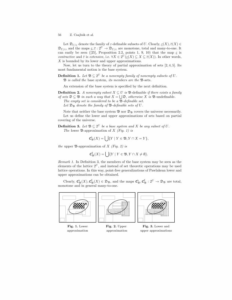
56 Z. Csajbok et al.
Let DU/ε denote the family of ε-definable subsets of U . Clearly, ε(X), ε(X) ∈DU/ε, and the maps ε, ε : 2U → DU/ε are monotone, total and many-to-one. Itcan easily be seen ([25], Proposition 2.2, points 1, 9, 10) that the map ε iscontractive and ε is extensive, i.e. ∀X ∈ 2U (ε(X) ⊆ X ⊆ ε(X)). In other words,X is bounded by its lower and upper approximations.
Now, let us turn to the theory of partial approximation of sets [2, 4, 5]. Itsmost fundamental notion is the base system.
Definition 1. Let B ⊆ 2U be a nonempty family of nonempty subsets of U .B is called the base system, its members are the B-sets.
An extension of the base system is specified by the next definition.
Definition 2. A nonempty subset X ⊆ U is B-definable if there exists a familyof sets D ⊆ B in such a way that X =
⋃D, otherwise X is B-undefinable.
The empty set is considered to be a B-definable set.Let DB denote the family of B-definable sets of U .
Note that neither the base system B nor DB covers the universe necessarily.Let us define the lower and upper approximations of sets based on partial
covering of the universe.
Definition 3. Let B ⊆ 2U be a base system and X be any subset of U .The lower B-approximation of X (Fig. 1) is
C[B(X) =⋃Y | Y ∈ B, Y ∩X = Y ,
the upper B-approximation of X (Fig. 2) is
C]B(X) =⋃Y | Y ∈ B, Y ∩X 6= ∅.
Remark 1. In Definition 3, the members of the base system may be seen as theelements of the lattice 2U , and instead of set theoretic operations may be usedlattice operations. In this way, point-free generalizations of Pawlakean lower andupper approximations can be obtained.
Clearly, C[B(X),C]B(X) ∈ DB, and the maps C[B,C]B : 2U → DB are total,monotone and in general many-to-one.
Fig. 1. Lower Fig. 2. Upper Fig. 3. Lower and
approximation approximation upper approximations
A Tool-Based Set Theoretic Framework for Concept Approximation 57
Proposition 1 ([6], Proposition 4.8). Let B ⊆ 2U be a base system. Then
1. ∀X ∈ 2U (C[B(X) ⊆ C]B(X));2. ∀X ∈ 2U (C[B(X) ⊆ X)—that is, C[B is contractive;
3. ∀X ∈ 2U (X ⊆ C]B(X)) if and only if⋃B = U—that is, C]B is extensive if
and only if B covers the universe.
Using the previous notations, the notion of the partial approximation spacecan be introduced.
Definition 4. The ordered quadruple 〈U,DB,C[B,C]B〉 is called the (weak) par-tial B-approximation space.
Let (P,≤P ) and (Q,≤Q) be two posets.
Definition 5. The pair of maps f : P → Q and g : Q → P forms a (regular)Galois connection between P and Q, in notation G(P, f, g,Q), if
∀p ∈ P ∀q ∈ Q (f(p) ≤Q q ⇔ p ≤P g(q)).
If P = Q, G(P, f, g, P ) is called a Galois connection on P .
Remark 2. Here we adopted the definition of Galois connection in which themaps are monotone. It is also called monotone or covariant form. For moredetails on Galois connections, see, e.g. [8]. Note that since Galois connectionsare not necessarily symmetric, the order of the maps is important.
It is well known fact ([13], Proposition 138) that upper and lower ε-approx-imations form a Galois connection G(2U , ε, ε, 2U ) on (2U ,⊆). Next theoremshows the conditions under which upper and lower B-approximations also forma Galois connection.
Theorem 1 ([6], Theorem 4.14). Let 〈U,B,C[B,C]B〉 be a partial B-approxi-mation space. The upper and lower B-approximations form a Galois connectionG(2U ,C]B,C[B, 2U ) on (2U ,⊆) if and only if the base system B is a partition ofU .
According to Proposition 1, point 3, X ⊆ C]B(X) if and only if the basesystem B covers the universe.
Definition 6. A subset X ⊆ U is B-approximatable if X ⊆ C]B(X), otherwiseit is said that X has a B-approximation gap.
A B-approximation gap may be interpreted so that our knowledge about theuniverse encoded in the base system is incomplete and not enough to approxi-mate X.
Definition 7. Let 〈2U ,DB,C[B,C]B〉 be a partial B-approximation space, andX be any subset of U .
The partial upper B-approximation of X is
∂C]B(X) =
C]B(X), if X is B-approximatable;undefined, otherwise.
(1)

58 Z. Csajbok et al.
There exists at least one nonempty B ∈ B B-set by Definition 2. ThenB ⊆ C]B(B) according to Definition 3. Hence, ∂C]B is defined on at least onenonempty subset of U .
Notice that C[B(X) ⊆ X ⊆ ∂C]B(X) holds provided X is B-approximatable.As Theorem 1 shows, the upper and lower B-approximations form a Galois
connection on (2U ,⊆) if and only if the base system B is a partition of U . Thequestion naturally arises whether the Galois connection could be generalizedso that the maps ∂C]B and C[B may form a Galois connection in any sense.Moreover, if the answer is yes, then what conditions have to be fulfilled by apartial B-approximation space so that ∂C]B and C[B form a Galois connection of
this special type. Recall that C[B is a total and ∂C]B is a partial map on 2U .To answer this question, first of all, we need a suitable modified notion of
Galois connections.
Definition 8 ([18], Definition 2.2.2). The pair of maps f : P → Q andg : Q → P forms a partial Galois connection between P and Q, denoted by∂G(P, ∂f, g,Q), if
1. f : P → Q is a monotone partial map,2. g : Q→ P is a monotone total map,3. f(g(q)) exists for all q ∈ Q, and4. ∀p ∈ P and ∀q ∈ Q such that f(p) is defined, f(p) ≤Q q ⇔ p ≤P g(q).
Remark 3. In [18], A. Mine actually introduced the concept of F-partial Galoisconnection ∂G(P, ∂f, g,Q) between the concrete domain P and the abstractdomain Q, where F is a set of concrete operators. We apply this notion in thesimplest form when P = Q = 2U and F = ∅. It is allowed by Mine’s definition.
Theorem 2 ([6], Theorem 4.22). Let 〈U,B,C[B,C]B〉 be a partial B-approxi-mation space.
The partial upper B-approximation and the lower B-approximation form apartial Galois connection ∂G(2U , ∂C]B,C[B, 2U ) on (2U ,⊆) if and only if the B-sets are pairwise disjoint.
A natural question is how we can form a base system from an arbitrary oneof which members are pairwise disjoint. In practice, this problem can be reducedto finite base systems. A possible way to construct such a base system is thefollowing.
First, let us form an intersection structure from an arbitrary finite basesystem. Formally, a nonempty family S ⊆ 2U is an intersection structure if∀S′( 6= ∅) ⊆ S (
⋂S′ ∈ S), i.e. it is closed under intersection but does not
contain U necessarily [7].Let us take an arbitrary finite base system B and create its intersection
structure IS(B) as the smallest set which satisfies the following two properties:
1. B ⊆ IS(B).2. If B′ ⊆ IS(B), then
⋂B′ ∈ IS(B).

A Tool-Based Set Theoretic Framework for Concept Approximation 59
Having given the intersection structure IS(B), we can create a family of setsISΠ(B) of which members are pairwise disjoint. ISΠ(B) is the smallest familyof sets which satisfies the following property:
If u ∈ U and B′ = B : B ∈ B ∧ u ∈ B, then⋂B′ ∈ ISΠ(B).
3 Rough Set Theory and Formal Concept Analysis
Let G and M denote a set of objects and a finite set of attributes, respectively.Note that the formal concept analysis allows that G and M to be empty sets,but the rough set theory does not.
3.1 Information Systems
First, we reformulate the rough set theory [9, 24]. Let S = 〈G,M, Vm∈M , f〉 bean information system, where G and M as before, Vm is a nonempty set of valuesof attribute m ∈M , and f : G×M → V =
⋃m∈M Vm is an information function
with ∀g ∈ G∀m ∈ M (f(g,m) ∈ Vm). Informally, f(g,m) represents the valuewhich object g takes at attribute m.
The information system is often represented by a table, as shown in Table 1.It is an information table containing a shortened student grade history from aninformation technology course held for hospital nurses at the Faculty of Health,University of Debrecen. It contains 20 students and their results in three home-work assignments, and one final examination.
Table 1. Information system Table 2. Information system
of a shortened student grade history of a shortened student grade history
(complete) (partial)
Student Hw1 Hw2 Hw3
Final
exam
S 1 1 1 1 1
S 2 1 1 2 2
S 3 1 1 1 1
S 4 1 2 1 1
S 5 1 1 1 1
S 6 1 1 2 1
S 7 4 1 3 1
S 8 2 4 1 2
S 9 1 3 1 2
S 10 1 1 3 1
S 11 2 1 1 2
S 12 1 1 1 1
S 13 1 2 1 1
S 14 1 1 2 3
S 15 4 3 3 4
S 16 2 1 1 4
S 17 2 2 2 4
S 18 4 4 3 3
S 19 4 3 3 2
S 20 4 4 3 4
Student Hw1 Hw2 Hw3
Final
exam
S 1 1 1 1 1
S 2 1 1 2 2
S 3 1 1 1 1
S 4 2 1
S 5 1 1 1 1
S 6 1 1 2 1
S 7 1 3 1
S 8 2 4 1 2
S 9 1 3 1 2
S 10 1 1 3 1
S 11 2 1 1 2
S 12 1 1 1 1
S 13 1 2 1 1
S 14 1 1 2 3
S 15 4 3 3 4
S 16 2 1 1 4
S 17 4
S 18 4 4 3 3
S 19 4 3 3 2
S 20 4 4 3 4

60 Z. Csajbok et al.
With each N ⊆M we associate an equivalence relation EN ⊆ G×G by
(g1, g2) ∈ EN if ∀n ∈ N (f(g1, n) = f(g2, n)).
If g ∈ G, then [g]ENis the equivalence class of EN containing g. Let G/N denote
the set of equivalence classes generated by EN .A concept X ⊆ G is EN -definable or EN -exact if X is a union of some
equivalence classes, otherwise X is EN -undefinable or EN -inexact.Lower and upper EN -approximations of X are:
EN (X) =⋃[g]EN
∈ G/N | [g]EN⊆ X,
EN (X) =⋃[g]EN
∈ G/N | [g]EN∩X 6= ∅.
3.2 Formal Context
In formal concept analysis a formal context is a triple 〈G,M,R〉 [11], where Gand M as above and R ⊆ G×M is a binary relation. Choosing
∀m ∈M (Vm = 0, 1) and f(g,m) =
1, if (g,m) ∈ R;0, otherwise
,
we may transform information systems into formal contexts. For instance, Table3 shows a formal context representation of the same example shown in Table 1.
Table 3. Formal context Table 4. Incomplete formal context
of a shortened student grade history of a shortened student grade history
Final
Student 1 2 3 4 5 1 2 3 4 5 1 2 3 4 5 exam
S 1 1 0 0 0 0 1 0 0 0 0 1 0 0 0 0 1
S 2 1 0 0 0 0 1 0 0 0 0 0 1 0 0 0 2
S 3 1 0 0 0 0 1 0 0 0 0 1 0 0 0 0 1
S 4 1 0 0 0 0 0 1 0 0 0 1 0 0 0 0 1
S 5 1 0 0 0 0 1 0 0 0 0 1 0 0 0 0 1
S 6 1 0 0 0 0 1 0 0 0 0 0 1 0 0 0 1
S 7 0 0 0 1 0 1 0 0 0 0 0 0 1 0 0 1
S 8 0 1 0 0 0 0 0 0 1 0 1 0 0 0 0 2
S 9 1 0 0 0 0 0 0 1 0 0 1 0 0 0 0 2
S 10 1 0 0 0 0 1 0 0 0 0 0 0 1 0 0 1
S 11 0 1 0 0 0 1 0 0 0 0 1 0 0 0 0 2
S 12 1 0 0 0 0 1 0 0 0 0 1 0 0 0 0 1
S 13 1 0 0 0 0 0 1 0 0 0 1 0 0 0 0 1
S 14 1 0 0 0 0 1 0 0 0 0 0 1 0 0 0 3
S 15 0 0 0 1 0 0 0 1 0 0 0 0 1 0 0 4
S 16 0 1 0 0 0 1 0 0 0 0 1 0 0 0 0 4
S 17 0 0 0 1 0 0 0 0 1 0 0 0 1 0 0 4
S 18 0 0 0 1 0 0 0 0 1 0 0 0 1 0 0 3
S 19 0 0 0 1 0 0 0 1 0 0 0 0 1 0 0 2
S20 0 0 0 1 0 0 0 0 1 0 0 0 1 0 0 4
Homework1 Homework2 Homework3
S20 0 0 0 1 0 0 0 0 1 0 0 0 1 0 0 4
Final
Student 1 2 3 4 5 1 2 3 4 5 1 2 3 4 5 exam
S 1 1 0 0 0 0 1 0 0 0 0 1 0 0 0 0 1
S 2 1 0 0 0 0 1 0 0 0 0 0 1 0 0 0 2
S 3 1 0 0 0 0 1
S 4 1 0 0 0 0 0 1 0 0 0 1 0 0 0 0 1
S 5 1 0 0 0 0 1 0 0 0 0 1 0 0 0 0 1
S 6 1 0 0 0 0 1 0 0 0 0 0 1 0 0 0 1
S 7 1 0 0 0 0 0 0 1 0 0 1
S 8 0 1 0 0 0 0 0 0 1 0 1 0 0 0 0 2
S 9 1 0 0 0 0 0 0 1 0 0 1 0 0 0 0 2
S 10 1 0 0 0 0 1 0 0 0 0 0 0 1 0 0 1
S 11 0 1 0 0 0 1 0 0 0 0 1 0 0 0 0 2
S 12 1 0 0 0 0 1 0 0 0 0 1 0 0 0 0 1
S 13 1 0 0 0 0 0 1 0 0 0 1 0 0 0 0 1
S 14 1 0 0 0 0 1 0 0 0 0 0 1 0 0 0 3
S 15 0 0 0 1 0 0 0 1 0 0 0 0 1 0 0 4
S 16 0 1 0 0 0 1 0 0 0 0 1 0 0 0 0 4
S 17 4
S 18 0 0 0 1 0 0 0 0 1 0 0 0 1 0 0 3
S 19 0 0 0 1 0 0 0 1 0 0 0 0 1 0 0 2
S 20 0 0 0 1 0 0 0 0 1 0 0 0 1 0 0 4
Homework3Homework1 Homework2
S 20 0 0 0 1 0 0 0 0 1 0 0 0 1 0 0 4

A Tool-Based Set Theoretic Framework for Concept Approximation 61
Given the formal context 〈G,M,R〉 we define
AB = m ∈M | ∀g ∈ A ((g,m) ∈ R), for A ⊆ G,
BC = g ∈ G | ∀m ∈ B((g,m) ∈ R), for B ⊆M,
called the polars of A, B, respectively [26].Informally, AB is the set of attributes common to all the objects in A, BC is
the set of all objects which possess all of the attributes in B.Given A ⊆ G and B ⊆ M we have A× B ⊆ R ⇔ A ⊆ BC ⇔ AB ⊇ B. The
pair (A,B) is called a formal concept if
A = BC and AB = B.
Formal concepts are usually ordered by inclusion on the first co-ordinateand/or reverse inclusion on the second:
(A1, B1) (A2, B2)⇔ A1 ⊆ A2 and B1 ⊇ B2 ⇔ A1 ⊆ A2 ⇔ B1 ⊇ B2.
Formal concepts with this ordering form a concept hierarchy for the context〈G,M,R〉 and denoted by B(G,M,R). The fundamental theorem of formal con-cept analysis states that B(G,M,R) with the ordering is a complete latticecalled the concept lattice [11].
4 A Tool-Based Set Theoretic Approximation Framework
Let U be any nonempty set. Let A+, A− ⊆ U be two nonempty subsets of U insuch a way that A+ ∩ A− = ∅. A+ and A− are called the positive and negativereference set, respectively. The adjectives positive and negative claim nothingelse but that the sets A+ and A− are well separated.
In general, the constraint A+ ∩ A− = ∅ is the only requirement for A+ andA−. Of course, additional relations between them may be supposed.
Furthermore, let T+ and T− ⊆ 2U be two nonempty finite families of subsetsof U . The members of T+ are called positive or T+-tools, whereas the membersof T− are called negative or T−-tools.
Requirements for positive and negatives tools are the following:
(T1) For each subset T+ ∈ T+ (resp., T− ∈ T−) it is easy to decide whetheran element of U belongs to T+ (resp., T−) or not.
(T2) Sets in T+ are not necessarily pairwise disjoint, neither are those in T−.(T3) T+ ∩ T− = ∅.(T4) Neither
⋃T+ nor
⋃T− covers U necessarily.
(T5) It is assumed that
∀T+1 , T+
2 ∈ T+ (T+1 ∩ T+
2 ∈ T+), and ∀T−1 , T−2 ∈ T− (T−1 ∩ T−2 ∈ T−),
i.e. the T+ and T− are closed under intersection.

62 Z. Csajbok et al.
Positive (resp., negative) tools provide an opportunity to locate or approxi-mate the positive (resp., negative) reference set. Positive and negative toolstogether also yield useful information about the reference sets. To do this, wecan use the following three partial approximation spaces relaying on T+ and T−:
〈U,DT+ ,C[T+ ,C]T+〉, 〈U,DT− ,C[T− ,C
]T−〉, 〈U,DT+∪T− ,C[T+∪T− ,C
]T+∪T−〉.
Within these spaces, any clump of observed objects can be approximatedwith the help of the lower and upper T+(T−-,T+ ∪ T−-)-approximations.
5 An Illustrative Example
To illustrate our framework let us see a simple example. We want to approxi-mately estimate the achievement of students and their results in the final ex-amination in higher education [20, 21]. We have at our disposal an informationtable (Table 5) containing the student grade history (5 = excellent, 4 = good, 3= fair, 2 = pass, 1 = fail).
Table 5. Information table with student grade history
Student Hw1 Hw2 Hw3
Final
exam
S 1 1 1 1 1
S 2 1 1 2 2
S 3 1 1 1 1
S 4 1 2 1 1
S 5 1 1 1 1
S 6 1 1 2 1
S 7 4 1 3 1
S 8 2 4 1 2
S 9 1 3 1 2
S 10 1 1 3 1
S 11 2 1 1 2
S 12 1 1 1 1
S 13 1 2 1 1
S 14 1 1 2 3
S 15 4 3 3 4
S 16 2 1 1 4
S 17 2 2 2 4
S 18 4 4 3 3
S 19 4 3 3 2
S 20 4 4 3 4
Positive tools:
T+Hw1=4 = S7, S15, S18, S19, S20
T+Hw2=4 = S8, S18, S20
T+Hw1=4∧Hw2=4 = S18, S20
Negative tools:
T−Hw1=1 =
S1, S2, S3, S4, S5, S6, S9, S10, S12, S13, S14T−Hw2=1 =
S1, S2, S3, S5, S6, S7, S10, S11, S12, S14, S16T−Hw3=1 =
S1, S3, S4, S5, S8, S9, S11, S12, S13, S16T−Hw1=1∧Hw2=1 =
S1, S2, S3, S5, S6, S10, S12, S14T−Hw1=1∧Hw3=1 = S1, S3, S4, S5, S9, S12, S13T−Hw1=2∧Hw3=1 = S1, S3, S5, S11, S12, S16T−Hw1=1∧Hw2=1∧Hw3=1 = S1, S3, S5, S12
Of course, there is no way to accurately measure the achievement of studentsand their success or failure on the final exam. Moreover, students cannot exactlyappreciate ‘what they know’ or ‘what they do not know’. However, with the

A Tool-Based Set Theoretic Framework for Concept Approximation 63
apparatus of partial approximation spaces, we can analyze student grade historycontained in Table 5 in order to understand how the results in assignmentsapproximately relate to success or failure on the final exam.
For the sake of simplicity, students’ success and failure on homework assign-ments or the final exam are measured by grade 4 and grade 1, respectively. Basedon these prerequisites, the positive tools (Fig. 4) and negative tools (Fig. 5) arethe following (see also Table 5):
T+ = T+Hw1=4, T
+Hw2=4, T
+Hw1=4∧Hw2=4,
T− = T−Hw1=1, T−Hw2=1, T
−Hw3=1, T
−Hw1=1∧Hw2=1, T
−Hw1=1∧Hw3=1,
T−Hw1=2∧Hw3=1, T−Hw1=1∧Hw2=1∧Hw3=1
U
S8
T+
Hw2=4
S18
S20
T+
Hw1=4
S19S15
S17
S16
S1 S3
S12S11
S5
S14
S6
S10
S2
S7 S4
S9
S13
U
S1
S14
S3 S12
S4S13S9
S6
S10
S2
S7
S16S11
T¡
Hw1=1
S5
T¡
Hw2=1
T¡
Hw3=1
S15S17 S18 S19 S20
S8
Fig. 4. Positive tools (homework = 4). Fig. 5. Negative tools (homework = 1).〈U,DT+ ,C[
T+ ,C]
T+〉 partial 〈U,DT− ,C[T− ,C]
T−〉 partial
approximation space approximation space
Students who have successful final exams can be evaluated with both positiveand negative tools (Fig. 6, Fig. 7):
– C[T+(XFinal exam=4) = ∅Informally: there is no combination of successful homework in which casethe final exam surely succeeds.
– C]T+(XFinal exam=4) = T+Hw1=4 ∪ T+
Hw2=4 ∪ T+Hw1=4∧Hw2=4
Informally: if one of the Homework 1, 2 or both of the two succeed, the finalexam possibly succeeds.
– C[T−(XFinal exam=4) = ∅Informally: there is no combination of failed homework in which case thefinal exam surely succeeds.
– C]T−(XFinal exam=4) = T−Hw3=1
Informally: if the Homework 3 fails, the final exam may succeed.

64 Z. Csajbok et al.
U
S8
T+
Hw2=4
S18
S20
T+
Hw1=4
S19S15
S17
S16
S1 S3
S12S11
S5
S14
S6
S10
S2
S7 S4
S9
XFinal exam=4
S13
U
S1
S14
S3 S12
S4S13S9
S6
S10
S2
S7
S16S11
T¡
Hw1=1
S5
T¡
Hw2=1
T¡
Hw3=1
S15
S17
S18 S19
S20
S8
XFinal exam=4
Fig. 6. Evaluation of successful final Fig. 7. Evaluation of successful final
exams with positive tools exams with negative tools
Students who have failed their final exams can also be evaluated with bothpositive and negative tools (Fig. 8, Fig. 9):
– C[T+(XFinal exam=1) = ∅Informally: there is no combination of successful homework in which casethe final exam surely fails.
– C]T+(XFinal exam=1) = T+Hw1=4
Informally: if the only Homework 1 succeeds, the final exam possibly fails(because, e.g., Homework 1 is the simplest part of the course).
– C[T−(XFinal exam=1) = T−Hw1=1∧Hw2=1∧Hw3=1
Informally: If all homework fail, the final exam surely fails.– C]T−(XFinal exam=1) =
⋃T−
Informally: if at least one homework fails, the final exam possibly fails.
U
S8
T+
Hw2=4
S18
S20
T+
Hw1=4
S19
S15
S17
S16S1 S3
S12
S11
S5
S14
S6
S10
S2
S7
S4
S9
XFinal exam=1
S13
U
S1
S14
S3 S12
S4S13S9
S6
S10
S2
S7
S16S11
T¡
Hw1=1
S5
T¡
Hw2=1
T¡
Hw3=1
S15S17 S18 S19 S20
S8
XFinal exam=1
Fig. 8. Evaluation of failed final exams Fig. 9. Evaluation of failed final exams
with positive tools with negative tools

A Tool-Based Set Theoretic Framework for Concept Approximation 65
Evaluations can also be carried out over positive and negative tools together:
– C[T+∪T−(XFinal exam=4) = ∅ (see Fig. 10) informally means that there is nocombination of successful or failed homework in which case the final examsurely succeeds.
– C]T+∪T−(XFinal exam=4) (see Fig. 10) informally means that if one of theHomework 1, 2 or both of the two succeed, in addition, even if one of theHomework 1, 3 or both of the two fail, then the final exam possibly succeed.
– C[T+∪T−(XFinal exam=1) (see Fig. 11) informally means that if at least onehomework fails, the final exam surely fails.
– C]T+∪T−(XFinal exam=1) (see Fig. 11) informally means that if at least onehomework fails, the final exam possibly fails even if the Homework 1 succeeds.
U
S8
T+
Hw2=4
S18
S20
T+
Hw1=4
S19S15
S17
T¡
Hw2=1
T¡
Hw3=1
S16
S1 S3
S12S11
S5
S14
S6
S10
S2
S7 S4
S9
XFinal exam=4
S13
C[T+∪T−(XFinal exam=4) = ∅
C]T+∪T−(XFinal exam=4)
= T+Hw1=4 ∪ T+
Hw2=4
∪T+Hw1=4∧Hw2=4
∪T−Hw2=1 ∪ T−Hw3=1
∪T−Hw2=1∧Hw3=1
Fig. 10. Evaluation of successful final exams with positive and negative tools
U
S1
S14
S3 S12
S4S13S9
S6
S10
S2
S7
S16S11
T¡Hw1=1
S5
T¡Hw2=1
T¡Hw3=1
S15S17 S18 S19 S20
XFinal exam=1
T+Hw1=4
S8
C[T+∪T−(XFinal exam=1)
= T−Hw1=1∧Hw2=1∧Hw3=1
C]T+∪T−(XFinal exam=1)
= T−Hw1=1 ∪ T−Hw2=1 ∪ T−Hw3=1
∪T−Hw1=1∧Hw2=1
∪T−Hw1=1∧Hw3=1
∪T−Hw2=1∧Hw3=1
∪T−Hw1=1∧Hw2=1∧Hw3=1
∪T+Hw1=4
Fig. 11. Evaluation of failed final exams with positive and negative tools

66 Z. Csajbok et al.
6 Conclusion
We have presented in this paper a tool-based set theoretic framework for conceptapproximation relying on partial approximation spaces. Positive features andtheir substantially negative features of observed objects can simultaneously beapproximated with the help of this framework.
We have drawn up a simplified example to demonstrate our approach. Wehave analyzed a student grade history and we have been able to evaluate thestudents’ achievement, exploring ‘what they know’ and/or ‘what they do notknow’, and understand how the results in homework assignments approximatelyrelate to success or failure on the final exam. Of course, a more subtle definitionof the notions of ‘success’ and ‘failure’ could result in a more subtle evaluation.A refined evaluation process can form a basis for quality insurance in highereducation properly building in the hierarchy of quality management.
Acknowledgement
The author would like to express his gratitude to the anonymous referees forreading the paper carefully and their insightful comments and suggestions.
References
1. Proceedings of the International Multiconference on Computer Science and Infor-mation Technology, IMCSIT 2009, Mragowo, Poland, 12-14 October 2009. PolskieTowarzystwo Informatyczne - IEEE Computer Society Press (2009)
2. Csajbok, Z.: Partial approximative set theory: A generalization of the rough settheory. In: Martin, T., Muda, A.K., Abraham, A., Prade, H., Laurent, A., Laurent,D., Sans, V. (eds.) Proceedings of SoCPaR 2010, December 7-10, 2010., CergyPontoise / Paris, France. pp. 51–56. IEEE (2010)
3. Csajbok, Z., Mihalydeak, T.: A general tool-based approximation framework basedon partial approximation of sets. In: Kuznetsov, S.O., et al. (eds.) Proceedings ofRSFDGrC 2011, June 25-27, 2011, Moscow, Russia. LNAI, vol. 6743, pp. 52–59.Springer-Verlag Berlin Heidelberg (2011)
4. Csajbok, Z., Mihalydeak, T.: On the general set theoretical framework of set ap-proximation. pp. 12–15 (2011), Proceedings of RST 2011, 14-16 September 2011,Milan, Italy (2011)
5. Csajbok, Z., Mihalydeak, T.: Partial approximative set theory: A generalization ofthe rough set theory. International Journal of Computer Information Systems andIndustrial Management Applications 4, 437–444 (2012)
6. Csajbok, Z.: Approximation of sets based on partial covering. Theoretical Com-puter Science 412(42), 5820–5833 (2011)
7. Davey, B.A., Priestley, H.A.: Introduction to Lattices and Order. Cambridge Uni-versity Press, Cambridge (2002)
8. Denecke, K., Erne, M., Wismath, S. (eds.): Galois Connections and Applications.Kluwer Academic Publishers (2004)
9. Duntsch, I., Gediga, G.: Statistical evaluation of rough set dependency analysis.International Journal of Human-Computer Studies 46(5), 589–604 (1997)

A Tool-Based Set Theoretic Framework for Concept Approximation 67
10. Ganter, B., Kuznetsov, S.O.: Formalizing hypotheses with concepts. In: Mineau,G., Ganter, B. (eds.) Proc. 8th Int. Conf. on Conceptual Structures, ICCC’2000.Lecture Notes in Artificial Intelligence, vol. 1867, pp. 342–356. Springer, Berlin(2000)
11. Ganter, B., Wille, R.: Formal concept analysis: Mathematical foundations.Springer, Berlin-Heidelberg (1999)
12. Gartmeier, M., Bauer, J., Gruber, H., Heid, H.: Negative knowledge: Understand-ing professional learning and expertise. Vocations and Learning: Studies in Voca-tional and Professional 1(2), 87–103 (2008)
13. Jarvinen, J.: Lattice theory for rough sets. In: Peters, J.F., Skowron, A., Duntsch,I., Grzyma la-Busse, J.W., Or lowska, E., Polkowski, L. (eds.) Transactions onRough Sets VI, LNCS, vol. 4374, pp. 400–498. Springer-Verlag (2007)
14. Keefe, R.: Theories of Vagueness. Cambridge Studies in Philosophy, CambridgeUniversity Press, Cambridge, UK (2000)
15. Kuznetsov, S.O.: Machine learning and formal concept analysis. In: Eklund, P.W.(ed.) Concept Lattices, Second International Conference on Formal Concept Anal-ysis, ICFCA 2004, Sydney, Australia, February 23-26, 2004, Proceedings. LectureNotes in Computer Science, vol. 2961, pp. 287–312. Springer-Verlag, Berlin Hei-delberg (2004)
16. Kuznetsov, S.O.: Galois connections in data analysis: Contributions from the sovietera and modern russian research. In: Ganter, B., Stumme, G., Wille, R. (eds.)Formal Concept Analysis, Foundations and Applications. LNAI, vol. 3626, pp.196–225. Springer (2005)
17. Marek, V.W., Truszczynski, M.: Approximation schemes in logic and artificial in-telligence. In: Peters, J.F., Skowron, A., Rybinski, H. (eds.) Transactions on RoughSets IX. LNCS, vol. 5390, pp. 135–144. Springer-Verlag (2008)
18. Mine, A.: Weakly Relational Numerical Abstract Domains. Ph.D. thesis, EcolePolytechnique, Palaiseau, France (December 2004)
19. Minsky, M.: Negative expertise. International Journal of Expert Systems 7(1), 13–19 (1994)
20. Narli, S., Ozelik, Z.A.: Data mining in topology education: Rough set data analysis.International Journal of the Physical Sciences 5(9), 1428–1437 (2010)
21. Narli, S., Yorek, N., Sahin, M., Usak, M.: Can we make definite categorization ofstudent attitudes? a rough set approach to investigate students implicit attitudinaltypologies toward living things. Journal of Science Education and Technology 19,456–469 (2010)
22. Pagliani, P., Chakraborty, M.: A Geometry of Approximation: Rough Set TheoryLogic, Algebra and Topology of Conceptual Patterns (Trends in Logic). SpringerPublishing Company, Incorporated (2008)
23. Parviainen, J., Eriksson, M.: Negative knowledge, expertise and organisations. In-ternational Journal of Management Concepts and Philosophy 2(2), 140–153 (2006)
24. Pawlak, Z.: Rough sets. International Journal of Computer and Information Sci-ences 11(5), 341–356 (1982)
25. Pawlak, Z.: Rough Sets: Theoretical Aspects of Reasoning about Data. KluwerAcademic Publishers, Dordrecht (1991)
26. Priestley, H.A.: Ordered sets and complete lattices: A primer for computer science.In: Backhouse, R.C., Crole, R.L., Gibbons, J. (eds.) Algebraic and CoalgebraicMethods in the Mathematics of Program Construction. LNCS, vol. 2297, pp. 21–78. Springer (2000)
27. Revett, K., Gorunescu, F., Salem, A.B.M.: Feature selection in parkinson’s disease:A rough sets approach. In: IMCSIT [1], pp. 425–428

68 Z. Csajbok et al.
28. Salem, A.B.M., Revett, K., El-Dahshan, E.S.A.: Machine learning in electrocar-diogram diagnosis. In: IMCSIT [1], pp. 429–433
29. Skowron, A.: Rough sets in perception-based computing. In: Pal, S.K., Bandy-opadhyay, S., Biswas, S. (eds.) Pattern Recognition and Machine Intelligence, FirstInternational Conference, PReMI 2005, Kolkata, India, December 20-22, 2005, Pro-ceedings. LNCS, vol. 3776, pp. 21–29. Springer (2005)
30. Skowron, A., Stepaniuk, J., Swiniarski, R.: Approximation spaces in rough-granularcomputing. Fundamenta Informaticae 100(1–4), 141–157 (2010)
31. Zadeh, L.A.: A new direction in AI: Toward a computational theory of perceptions.AI Magazine 22(1), 73–84 (2001)
Decision Aiding Software Using FCA
Florent Domenach and Ali Tayari
Computer Science Department, University of Nicosia, 46 Makedonitissas Av.,P.O.Box 24005, 1700 Nicosia, Cyprus, [email protected]
Abstract. The consensus problem arises from social choice theory andsystematic biology where we are looking for the common informationshared by a series of trees. In this paper we present a decision aidingsoftware to help systematic biologist to choose the consensus functionthe most appropriate for their need. This software is based on a previousstudy between consensus functions and axiomatic properties, and theirunderlined concept lattice.
1 Introduction
The consensus problem, which [11] deemed a ”problem for the future”, consistsof summarizing a series of structures, usually trees, into one representative struc-ture. Axiomatic studies of consensus functions is often [26] described as an ”idealsituation [in which] the researcher formulates a list of desirable axioms that aconsensus function should satisfy, and search for the best method that satisfiesthese axioms” [33]. We present here a software following this approach almostto the letter. Unfortunatly, it is still missing critical GUI features and is notavailable yet.
The motivation for the software is originating from the separation existingbetween theorizers and practitioners of consensus theory, what [7] denotes asabstract consensus theory and concrete consensus theory. On one hand, math-ematicians are developing sophisticated mathematical tools. The modern devel-opment of the consensus problem originates from Arrow’s work [3] (followedby [25]) who considered the problem of aggregating votes and showed that anyvoting system is either inconsistent, arbitrary or unstable. Since then, a lot offunctions, together with a set of equivalent axioms, were developed (see [15, 22]for a comprehensive survey).
On the other hand, practitioners like systematic biologists are rarely usingmore than a handful of consensus functions. If you consider the most popularsoftware available like PAUP∗1 [37] (majority), PHYLIP2 [20] (majority, strict),or COMPONENT 2.03 [30] (strict, majority-rule, loose, Nelson and Adams con-sensus trees), only a handful are available for use. It was pointed out [38] thatthis gap between the two communities was detrimental to both.
1 http://paup.csit.fsu.edu/2 http://evolution.genetics.washington.edu/phylip.html3 http://taxonomy.zoology.gla.ac.uk/rod/cpw.html
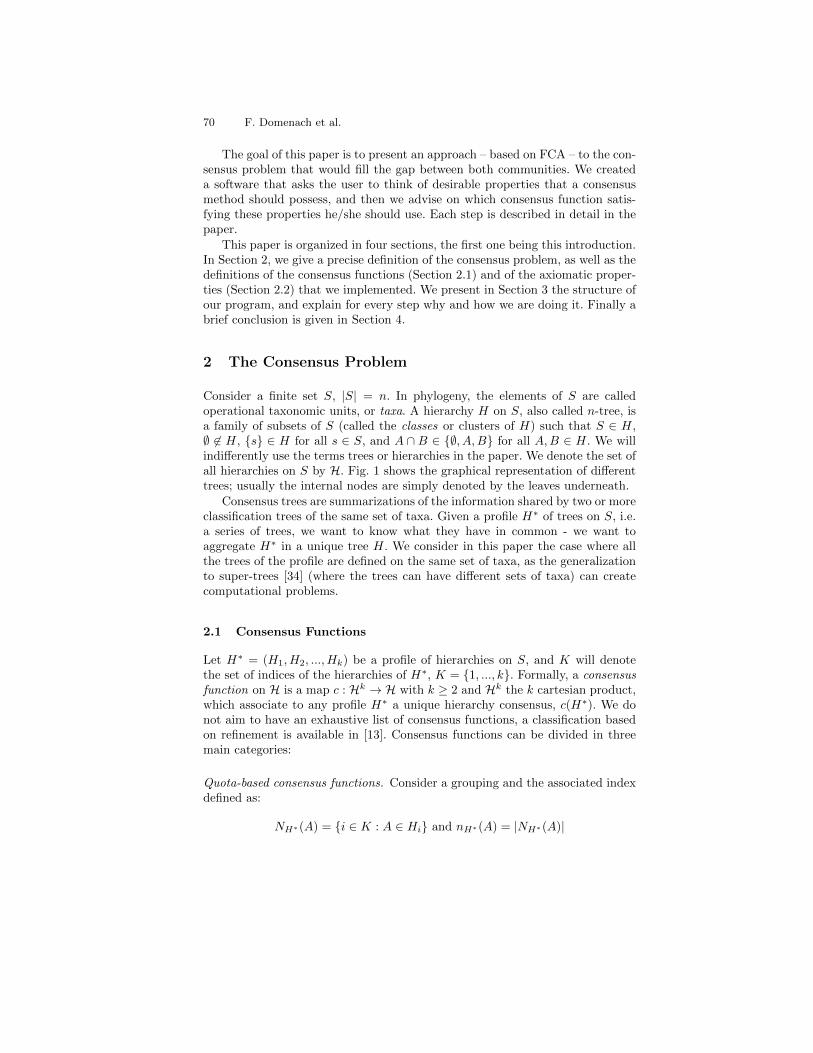
70 F. Domenach et al.
The goal of this paper is to present an approach – based on FCA – to the con-sensus problem that would fill the gap between both communities. We createda software that asks the user to think of desirable properties that a consensusmethod should possess, and then we advise on which consensus function satis-fying these properties he/she should use. Each step is described in detail in thepaper.
This paper is organized in four sections, the first one being this introduction.In Section 2, we give a precise definition of the consensus problem, as well as thedefinitions of the consensus functions (Section 2.1) and of the axiomatic proper-ties (Section 2.2) that we implemented. We present in Section 3 the structure ofour program, and explain for every step why and how we are doing it. Finally abrief conclusion is given in Section 4.
2 The Consensus Problem
Consider a finite set S, |S| = n. In phylogeny, the elements of S are calledoperational taxonomic units, or taxa. A hierarchy H on S, also called n-tree, isa family of subsets of S (called the classes or clusters of H) such that S ∈ H,∅ 6∈ H, s ∈ H for all s ∈ S, and A ∩ B ∈ ∅, A,B for all A,B ∈ H. We willindifferently use the terms trees or hierarchies in the paper. We denote the set ofall hierarchies on S by H. Fig. 1 shows the graphical representation of differenttrees; usually the internal nodes are simply denoted by the leaves underneath.
Consensus trees are summarizations of the information shared by two or moreclassification trees of the same set of taxa. Given a profile H∗ of trees on S, i.e.a series of trees, we want to know what they have in common - we want toaggregate H∗ in a unique tree H. We consider in this paper the case where allthe trees of the profile are defined on the same set of taxa, as the generalizationto super-trees [34] (where the trees can have different sets of taxa) can createcomputational problems.
2.1 Consensus Functions
Let H∗ = (H1, H2, ...,Hk) be a profile of hierarchies on S, and K will denotethe set of indices of the hierarchies of H∗, K = 1, ..., k. Formally, a consensusfunction on H is a map c : Hk → H with k ≥ 2 and Hk the k cartesian product,which associate to any profile H∗ a unique hierarchy consensus, c(H∗). We donot aim to have an exhaustive list of consensus functions, a classification basedon refinement is available in [13]. Consensus functions can be divided in threemain categories:
Quota-based consensus functions. Consider a grouping and the associated indexdefined as:
NH∗(A) = i ∈ K : A ∈ Hi and nH∗(A) = |NH∗(A)|
Decision Aiding Software Using FCA 71
a bc d e
(H1)
a bc d e
(H2)
a bc d e
(H3)
a bc d e
(HStrict)
a bc d e
(HMaj)
a bc d e
(HLoose)
Fig. 1. Different trees defined on the set of taxa S = a, b, c, d, e. For the profileH∗ = (H1, H2, H3), the strict consensus tree is given by (HStrict), the majority by(HMaj) and the loose by (HLoose)
We associate the consensus function c(p) : Hk → H to the index nH∗ for any p ∈K. A subset A is called p-frequent if nH∗(A) ≥ p, and the p-frequent consensusof H∗, denoted as c(p)(H
∗), is the family of all p-frequent subsets. Quota-basedconsensus functions are particular cases of federation consensus functions [23].Recall that a federation (simple game) is a family F of subsets of K such thatA ∈ F , B ⊇ A imply B ∈ F . A federation consensus function cF is then definedas cF (H∗) = ∨S∈F (∩i∈SHi). If we take the simple case where, for some j ∈ K,F = S ⊆ K : j ∈ S, we have cF (H∗) = Hj , a single hierarchy dictating theresult of the consensus, the so called projection consensus function.
Projection: ∃j ∈ K : Prj(H∗) = Hj
When we extend this to a subset J of K, we have the oligarchic consensusfunction using F = S ⊆ K : J ⊆ S, and cF (H∗) =
⋂j∈J Hj .
Oligarchy: ∃J ⊆ K : Ol(H∗) =⋂
j∈JHj
In the family of quota-based consensus functions, one can notice c(k)(H∗) =⋂
i∈K Hi the set of classes present in all trees of the profile, i.e. the strict con-sensus function [36]. In Fig. 1, (HStrict) is the strict consensus of the profile(H1, H2, H3).
Strict: Str(H∗) =⋂
i∈KHi
If we take p = dk+12 e, the smallest natural number greater than k
2 , we have themajority consensus function [24] which considers clusters appearing in at least

72 F. Domenach et al.
half of the trees. An example of the majority consensus function is given in Fig.1, where (HMaj) = Maj(H1, H2, H3).
Majority: Maj(H∗) = X ⊆ S : nH∗(X) >k
2
Unfortunately, if p is less than dk+12 e, it cannot be guaranteed that the resulting
family will be a tree. In order to keep the structure of a tree, different strategiescan be used.
Frequency-based consensus functions A first approach considers the idea of com-patibility, i.e. two sets A and B are compatible if A ∩B ∈ ∅, A,B, denoted asA‖B, and a set A is compatible with a hierarchy H if it is compatible with everycluster of H (or, equivalently, if A ∪ H ∈ H). We then can define a consensusfunction called loose consensus [6] (originally called combinable component [12],also called semi-strict) which considers subsets as long as they are compatiblewith every tree of the profile. Fig. 1 shows (HLoose), the loose consensus treeobtained from (H1, H2, H3).
Loose: L(H∗) =⋃X ⊆ S : ∃j ∈ K,X ∈ Hj and ∀i ∈ K,X ∪Hi ∈ H
The loose consensus function was extended by [18] to two different consensusfunctions. The first one is combining the classes obtained by the majority con-sensus function with those of the loose consensus function:
Loose and Majority Function Property: LM(H∗) = Maj(H∗) ∪ L(H∗)
The second extension is to add classes that are more often compatible than not.Define NH∗(X) = i ∈ K : X ∪Hi 6∈ H as the set of trees not compatible witha subset X, then the majority (+) consensus function will take subsets that aremore often compatible than incompatible. It obviously contains all the classesobtained by the majority function and by the loose function.
Majority-rule (+) : Maj+(H∗) = X ⊆ S : |NH∗(X)| > |NH∗(X)|
Consider the weight function w(X) = nH∗(X)− 1 on classes. The Nelson-Pageconsensus tree is the tree constructed from the clique G containing the com-ponents most frequently replicated in the profile. If two or more cliques havethe same, maximal number of replications of components, then the consensustree is constructed from those components common to all those cliques. In theliterature, the Nelson-Page tree [27, 29] has often been confused with the strictconsensus tree.
The frequency difference consensus function consider the subsets of S thatare more frequent than any other subsets non-compatible.
Freq. Diff.: FD(H∗) = X : nH∗(X) > maxY not compatible with X
nH∗(Y )
Previous consensus functions may miss some structural features of the trees,particularly if the data is noisy. For example, a desirable feature would be that

Decision Aiding Software Using FCA 73
if two taxa are closer than a third one, we want these two taxa to be separatedfrom the third one in the consensus hierarchy - which is what Adams’ function [1]achieves. Historically the first one, an Adams consensus tree contains the nestingscommon to all trees in a profile. X nests in Y in H, denoted as X <H Y if andonly if X ⊂ Y and there is Z ∈ H such that X ⊆ Z and Y 6⊆ Z. π(H) is themaximal cluster partition for H with blocks equal to the maximal clusters of H.Adams’ consensus function is best described algorithmically (from [13]):
Procedure AdamsTree(H1, ...,Hk)Construct π(H), the product of π(H1), ..., π(Hk).For each block B of π(H) do
AdamsTree(H1|B , ...,Hk|B)
Distance-based consensus functions Another consensus family is based on dis-tance, either as a height function, or as distance between trees. Durchschnitt [28]consensus function takes the intersection of all classes at the same height. Thecanonical height η0(X) of a class X ⊆ S is defined as η0(S) = 0 and η0(X) = h ifand only if there is a maximal sequence S ⊃ X1 ⊃ ... ⊃ Xh−1 ⊃ Xh = X. Defineω = mini∈KmaxX∈Hiη0(X) as the height of the smallest tree of the profile.
Durchschnitt: Dur(H∗) =
ω⋃
j=1
⋂
i∈KXi : Xi ∈ Hi and η0(Xi) = j
The median and asymmetric median consensus functions both use a distancebetween trees, i.e. a distance on H. The median consensus is the tree minimizingthe distance of the symmetric difference from it to every tree of the profile.The median consensus was extensively studied, particularly in the case of semi-lattices [35] (as trees can be seen as semi-lattices).
Median: Med(H∗) = minH∈H
k∑
i=1
|H4Hi|
The asymmetric median consensus [32] on the other hand is the tree minimiz-ing the distance between each tree and the consensus tree, i.e. minimizing thenumber of classes in Hi that are not present in c(H∗).
Asymmetric Median: AMed(H∗) = minH∈H
k∑
i=1
|Hi −H|
2.2 Axiomatic Properties of Consensus Functions
Historically, consensus functions were studied through a series of (desirable) ax-ioms proved to be equivalent to the function. Arrow’s pioneer work proved theimpossibility of a non-dictatorial consensus function satisfying fundamental ax-ioms (transitivity, Pareto and independence of irrelevant alternatives) on linear

74 F. Domenach et al.
orders. We implemented a series of axioms that a user may find desirable orundesirable.
A consensus function is Pareto relatively to a specific kind of relationships(classes, triplets, nestings) when the consensus tree will contain the relationshippresent in all the trees, i.e. will contain the intersection of the trees of the profilewith respect to the relationship. For example, when we are interested in thecommon classes, we have the Pareto optimal [31] axiom:
Pareto Optimality: (∀X ⊆ S)(X ∈k⋂
i=1
Hi ⇒ X ∈ c(H∗))
Trees can also be defined [14] through triplets ab|c, a, b, c ∈ S, denoting thegrouping of a and b relative to c. We say that ab|c ∈ H if there exists a classX ∈ H such that a, b ∈ X but c 6∈ X. The Pareto property on triplets is that acommon separation of two taxa from a third taxon among every input tree mustbe respected and applied in the consensus tree.
Ternary Pareto Optimality: (∀x, y, z ∈ S)((∀i ∈ K)(xy|z ∈ Hi)⇒ xy|z ∈ c(H∗))
Adams [2] extended that idea to nestings, where if two clusters are separatedfrom each other in every input tree, therefore they must also be separated in theconsensus tree:
Nesting Preservation: (∀∅ 6= X,Y ⊆ S)((∀i ∈ K)(X <HiY )⇒ (X <c(H∗) Y ))
Conversely, a consensus function is co-Pareto for a particular relationship if onecan find every relationship of that kind of the consensus tree in one or more treeof the profile. Every cluster from the consensus tree must appear in at least oneof the input tree, or in other words it should be a member of the union of allinput trees. We will consider here only co-Pareto optimally for classes.
co-Pareto Optimality: (c(H∗) ⊆k⋃
i=1
Hi)
In order to characterize his consensus function, Adams introduced a reciprocalproperty of nesting preservation, although stronger than just a co-Pareto prop-erty. It states that if two subsets are nested in the consensus tree, they must benested in all the trees of the profile.
Strong Presence: (∀∅ 6= X,Y ⊆ S)(X <c(H∗) Y ⇒ (∀i ∈ K)(X <HiY ))
It happened that Strong Presence property was too constraining, so instead ofconsidering all possible nested subsets, Adams considered only the nested classes.Any two clusters of the consensus tree that are separated from each other mustalso be separated in every input tree.
Qualified Strong Presence: (∀X,Y ∈ c(H∗))(X <c(H∗) Y ⇒ (∀i ∈ K)(X <HiY ))

Decision Aiding Software Using FCA 75
Qualified strong presence was weakened to consider the clusters of the consensustree to be nested in S in each tree of the profile:
Upper Strong Presence: (∀X ∈ c(H∗))(X <c(H∗) S ⇒ (∀i ∈ K)(X <Hi S))
The dictatorship property (an input tree dictates over the consensus tree byhaving all of its clusters included in the consensus tree) is often consider unde-sirable; however, this can change if there is a particular tree that can be consideran oracle, i.e. for which we want the consensus tree to refine it.
Dictatorship: (∃j ∈ K)(∀X ⊆ S)(X ∈ Hj ⇒ X ∈ c(H∗))Another desirable property, also called faithful, is the following: for every groupof clusters containing only one cluster from each input tree there must be acluster in the consensus tree such that it includes the intersection of the groupof the group of clusters and it is included in the union of the groups of the groupof clusters.
Betweenness: (∀i ∈ K with Xi ∈ Hi)(∃Y ∈ c(H∗))(k⋂
i=1
Xi ⊆ Y ⊆k⋃
i=1
Xi)
3 Decision Aiding Software
We used Formal Concept Analysis (FCA) [21] as our formal background. FCA isparticularly suitable as it provides a structure on the power set of attributes, herethe consensus functions and axioms, and allow calculations of distances on thatstructure. Since we assume the reader familiar with FCA, we will only brieflyrecall main terminologies and results used in our program: a formal context(G,M, I) is defined as a set G of objects, a set M of attributes, and a binaryrelation I ⊆ G × M . (g,m) ∈ I is read as ”object g has attribute m”. Tothis formal context, one can associate to a set of objects A ⊆ G its intensionA′ = m ∈M : ∀g ∈ A, (g,m) ∈ I of all properties shared by A. Dually, we candefine B′ = g ∈ G : ∀m ∈ B, (g,m) ∈ I, the extension of a set of propertiesB ⊆ M . A pair (A,B), A ⊆ G,B ⊆ M , is a formal concept if A′ = B andB′ = A. The set of all formal concepts, ordered by inclusion, forms a lattice [5],called concept lattice. For more terms and definitions on lattice theory, one canrefer to [10, 16].
This D.A. software has three different functional layout (see Fig. 2): a pre-processing is first done on consensus functions and axioms in order to create thecontext that then will be used, with the associated lattice, in order to adviseusers on which consensus function to use. The last layer is concerned with theobtainment of the tree itself from some input profile.
3.1 Pre-processing
The first layer of the D.A. software concerns the pre-processing of the data thatwill be used. In order to insure scientific validity of the decision aiding, we imple-mented the previous consensus functions of Sec. 2.1 and the axiomatic properties

76 F. Domenach et al.
Fig. 2. D.A. software functional layout.
of Sec. 2.2 in C++ on a laptop Intel Core i5, 2.3 GHz. Initially, it generates allpossible hierarchies based on a given set of n taxa, and traverses through all pos-sible profiles of k hierarchies, together with all possible consensus trees. Thenwe exhaustively list what we called configurations, each configuration is a pairconsisting of a profile and a consensus tree. Every configuration was systemati-cally compared against axiomatic properties and consensus functions in order tocreate a first (raw) context. Attributes of the context are the consensus functionsand the axiomatic properties, while the objects are every possible configuration.We discussed in [17] the implications generated by the context.
During the pre-processing phase, we encountered a series of computationalchallenges, as the number of n-trees grows exponentially [19] and some consen-sus functions are NP-hard [32]. We were able to exhaustively investigate theconfigurations only up to n = 5, for which we obtained around 9.57× 10¹² con-figurations. Since the running time of the simulation increases exponentially withslight addition to n or k, in order to have partial results, controlled randomlyselected configurations were chosen in order to have a more accurate - and so amore refine - context.
3.2 Underlined Structure
Given the number of objects in our context (over one trillion), we first eliminateduplicates. If several configurations share the same attributes, we simply keepthe first one as representative. No information is lost as we are interested in

Decision Aiding Software Using FCA 77
the structure of the attributes, and the objects (the configurations) sole purposeis to systematically investigate this structure. Our simplified context has 5379objects for 23 attributes, and Fig. 3 shows the overall concept lattice, having3718 concepts. In order to derive the lattice, we followed The Next Closure [21]algorithm. This algorithm uses the lectic order on the set of attributes M , whichis a total order on P(M). Given two subsets A and B of M , A is said to belectically smaller than B at position i, and we denote it by A ≺i B, if and onlyif i = min(A∆B) and i ∈ B. Finally, we say that A is lectically smaller than Bif A = B or A ≺i B for some i ∈ K. We used Next Closure algorithm as it is anefficient and easy to implement.
Fig. 3. Concept lattice associated with the configurations with minimal labeling of theproperties (drawn with ConExp [39]).

78 F. Domenach et al.
After constructing the list of concepts and listing them in ascending order,the program also keeps track of the children and parents of each concept ofthe lattice. The user can then select a set of axiomatic properties dependingon the one he/she finds desirable or undesirable: each axiom can be preferred(positive), disliked (negative), or neutral. Based on that input, the programfinds the meet of the selected properties, i.e. the concept C associated to his/herchoices. Concept C is the smallest concept containing all the positive user’schoices and no negative ones if it exists. If the user’s choices are conflicting, i.e.C doesn’t exist, positive choices will be given priority over negative ones.
3.3 Distances in the lattice
In order to advise which consensus function would be suitable depending on theuser’s choices, for each consensus function, we first find the smallest concepts Ci
containing that consensus function. Then we used different distances between C(the concept representing the user’s choice) and each Ci (the concepts associatedwith consensus function i) in order to find the consensus function the closest tothe user’s choice. The use of different distances lets the user freely choose whichdistance is more suitable.
We can consider two types of distances in a lattice: distances based on con-cepts and distances on the covering graph (or Hasse diagram) of the lattice. Forthe first type, we used the distance of the symmetric difference between con-cepts, d1(C,Ci) = |C∆Ci|, i.e the number of properties present in either C orCi but not in both. For the second type, distances in the covering graph, weconsidered four distinct distances:
– Any Path Distance: weight of the shortest path (topological distance) be-tween the corresponding attribute concepts; the closer the two concepts arein the graph, the greater their likelihood.
– Any Path Distance Without ⊥L and >L: we remove the top and the bot-tom concepts of the lattice to compute the topological distance because suchconcepts don’t bear any information (even if 1L can have attributes associ-ated, it still doesn’t have any meaning). It is particularly important whenwe consider the co-atoms of the lattice (such as Pareto Optimal or co-ParetoOptimal, see Fig. 3), as the shortest path could go through 1L and short-circuit the ”real” distance.
– Meet Distance: It is the topological distance between C and Ci passingthrough their meet, i.e. the distance from C to C ∧ Ci plus the distancefrom Ci to C ∧ Ci.
– Join Distance: Dual to the meet distance, it is the topological distance be-tween C and Ci passing through their join.
Since each previous distance has its own advantages and disadvantages, we alsoimplemented a weighted average distance for which the user can freely assignthe weights. It is a weighted average of all the above distances based on user’spreference. Fig. 4 shows an example of user’s choice and the advised consensusfunction.

Decision Aiding Software Using FCA 79
Fig. 4. Screen shot of the second layer of the software, with an example of user’schoices.
3.4 Decision Aiding
In the third layer, the D.A. Software recognizes input trees which are givenin Newick format. The Newick tree format is a well-known representation ofgraph-theoretical trees which denotes trees using parentheses and commas. Thesimplicity and standard nature of Newick makes it a suitable method for scien-tists to provide the software with their input. There are several ways throughwhich trees can be represented, however the representation that contains onlythe information about the leaves are recognized as the valid ones. For example, inFig. 1, (H1) has the Newick format (((a, c), b), d, e), while (H2) is ((a, c), (b, d, e)).
Upon selection of consensus functions by the user, the D.A. software generatesthe unique (or set of all possible consensus trees) for the selected functions, sothat the user can compare them with each other. Using this feature, the user isable to find out which model would be more suitable for the nature of their work,for which he/she will be provided with respective consensus tree(s). This allowsthe user to have a narrowed list of candidates for the representative consensustrees as well as having a hands-on experience to find out the most suitablefunctional property and consensus tree.
4 Conclusion and Future Work
In this paper, we presented a decision aiding software which explore via FormalConcept Analysis the space of consensus functions and their axioms. It providesthe user with means to generate consensus tree(s) representative(s) dependingon their choices. It initially imports the raw context obtained via pre-processing,constructs the associated lattice and, depending on the user’s preferences, advise

80 F. Domenach et al.
based on distances in the lattice on which function to use. Upon selection offunctions, the program generates the consensus trees of the collection of user’sinput tree using selected functional properties.
In continuation of this project, we are planning to expand the capabilitiesof this software. Firstly, besides the (rooted) trees that are currently supportedas input and output, the program will be able to support super-trees as wellas unrooted trees as its input and output. Another possibility would be theaddition of other types of structures of sets such as pyramids [9], weak-trees[4], and, more generally, lattices. In addition, the concept of independence andneutrality as axiomatic properties are planned to be incorporated. Moreover,other commonly used consensus functions are going to be added to the result,therefore with a further refined and exhaustive approach, the program’s precisionand usefulness would be improved.
References
[1] Adams III, E.N.: Consensus Techniques and the Comparison of Taxonomic Trees.Systematic Zoology 21 (1972) 390–397
[2] Adams III, E.N.: N-trees as nestings: Complexity, similarity, and consensus. J.Classif 3 (1986) 299-317
[3] Arrow, K.J.: Social Choice and Individual Values. Wiley, New York (1951)
[4] Bandelt, H.-J., Dress, A.: Weak hierarchies associated with similarity measures: anadditive clustering technique Bull. Math. Biology 51 (1989) 133-166
[5] Barbut, M., Monjardet, B.: Ordres et classification: Algebre et combinatoire (tomeII). Hachette, Paris (1970)
[6] Barthelemy, J.-P., McMorris, F.R., Powers, R.C: Dictatorial consensus functionson n-trees. Math. Soc. Sci. 25 (1992) 59-64
[7] Barthelemy, J.-P., Brucker, F.: Average Consensus in Numerical Taxonomy. InData analysis, Eds. W. Gaul, O. Opitz, and M. Schader, Springer (2000) 95-104
[8] Bertrand, P.: Set Systems and Dissimilarities. Europ. J. Combinatorics 21 (2000)727-743
[9] Bertrand, P., Diday, E.: A visual representation of compatibility between an orderand a dissimilarity index: the pyramids. Comput. Stat. Quart. 2 (1985) 31-44
[10] Birkhoff, G.: Lattice Theory, 3rd ed. Amer. Math. Soc., Providence (1967)
[11] Bock, H.H.: Classification and clustering: Problems for the future. In Diday, E.,Lechevallier, Y., Schader, M., Bertrand, P., Burtschy, B.: New approaches in clas-sification and data analysis. Springer-Verlag, Berlin (1994) 3–24
[12] Bremer, K.: Combinable component consensus. Cladistics 6 (1990) 369-372
[13] Bryant, D.: A Classification of Consensus Methods for Phylogenetics. In: Janowitz,M., Lapointe, F.J., McMorris, F., Mirkin, B., Roberts, F. (eds.) Bioconsensus,DIMACS (2003) 163-184
[14] Colonius, H., Schulze, H.-H.: Tree structure for proximity Data. Brit. J. of Math.Stat. Psych. 34 (1981) 167-180
[15] Day, W.H.E., McMorris, F.R.: Axiomatic Consensus Theory in Group Choice andBiomathematics. Siam, Philadelphia (2003)
[16] Davey, B.A., Priestley, H. A.: Introduction to Lattices and Order, 2nd ed. Cam-bridge University Press (2002)
Decision Aiding Software Using FCA 81
[17] Domenach, F., Tayari, A.: Implications of Axiomatic Consensus Properties. Toappear (2012)
[18] Dong, J., Fernandez-Baca, D., McMorris, F.R., Powers. R.C.: An Axiomatic Studyof Majority-rule (+) and associated Consensus Functions on Hierarchies. Disc. App.Math. 159 (2011) 2038-2044
[19] Felsenstein, J.: The Number of Evolutionary Trees. Syst. Zool. 27 (1978) 27-33[20] Felsenstein, J.: PHYLIP - Phylogeny Inference Package (Version 3.2). Cladistics
5 (1989) 164-166[21] Ganter, B., Wille, R.: Formal Concept Analysis : Mathematical Foundations.
Springer (1996)[22] Hudry, O., Monjardet, B.: Consensus Theories. An Oriented Survey. Math. Sci.
hum 190 (2010) 139-167[23] Leclerc, B. Monjardet, B.: Latticial theory of consensus. In: Barnett, V., Moulin,
H., Salles M., Schofield N. (eds.) Social choice, Welfare and Ethics. CambridgeUniversity Press, Cambridge (1995) 145-159
[24] Margush, T., McMorris, F.R.: Consensus n-trees. Bull. Math. Biol. 43 (1981)239-244
[25] May, K.O.: A Set of Independent Necessary and Sufficient Conditions for SimpleMajority Decision. Econometrica 20 (1952) 680-684
[26] McMorris, F.R.: : Axioms for consensus functions defined on undirected phyloge-netic trees. Math. Biosciences 74 (1985) 77-80
[27] Nelson, G.: Cladistic analysis and synthesis: Principles and definitions, with ahistorical note on Adanson’s Famille des Plantes (1763-1764). Syst. Zool. 28 (1979)1-21
[28] Neumann, D.A.: Faithful consensus methods for n-trees. Math. Biosci 63 (1983)271-287
[29] Page, R.D.M.: Tracks and Trees in the Antipodes: A Reply to Humphries andSeberg. Syst. Zool. 39 (1990) 288-299
[30] Page, R.D.M.: User’s manual for COMPONENT, Version 2.0. Natural HistoryMuseum, London (1993)
[31] Pareto, V.: Cours d’economie politique. F. Rouge, Lausanne (1896)[32] Phillips, C., Warnow, T.J.: The aymmetric median tree - A new model for building
consensus trees. Disc. App. Math. 71 (1996) 311-335[33] Powers, R.C., White, J.M.: Wilson’s theorem for consensus functions on hierar-
chies. Disc. Appl. Math. 156 (2008) 1321–1329[34] Semple, M., Steel, C.: A supertree method for rooted trees. Disc. App. Math. 105
(2000) 147-158[35] Sholander M.: Medians, Lattices, and Trees. Proceedings of the American Math-
ematical Society 5 (1954) 808-812[36] Sokal, R.R., Rohlf, F.J., Taxonomic congruence in the Leptopodomorpha re-
examined. Syst. Zool. 30 (1981) 309-325[37] Swofford, D.L.: PAUP: Phylogenetic Analysis Using Parsimony, version 3.0. Illinois
Natural History Survery, Champaign (1990)[38] Wilkinson, M., Thorley, J.L., Pisani, D.E., Lapointe, F.-J., McInerney, James O.:
Some Desiderata for Liberal Supertrees. In: Phylogenetic Supertrees: CombiningInformation to Reveal the Tree of Life, Kluwer Academic Publishers (2004) 564-582
[39] Yevtushenko, S.A.: System of data analysis ”Concept Explorer”. Proceedings ofthe 7th national conference on Artificial Intelligence KII-2000, Russia (2000) 127-134
Analyzing Chat Conversations of Pedophileswith Temporal Relational Semantic Systems
Paul Elzinga1, Karl Erich Wolff2, Jonas Poelmans3,4, Guido Dedene3,5, andStijn Viaene3,6
1 Amsterdam-Amstelland PoliceJames Wattstraat 84, 1097DM Amsterdam, The Netherlands
[email protected] Ernst-Schroder-Center, Darmstadt University of Technology
Schloßgartenstr. 7, D-64289 Darmstadt, [email protected]
3 K.U.Leuven, Faculty of Business and Economics, Naamsestraat 69, 3000 Leuven,Belgium
4 National Research University Higher School of Economics (HSE)Pokrovskiy boulvard 11, 101000 Moscow, Russia
[email protected] Universiteit van Amsterdam Business School
Roetersstraat 11, 1018 WB Amsterdam, The [email protected]
6 Vlerick Leuven Gent Management School, Vlamingenstraat 83, 3000 Leuven,Belgium
Abstract. Grooming is the process by which pedophiles try to find chil-dren on the internet for sex-related purposes. In chat conversations theymay try to establish a connection and escalate the conversation towardsa physical meeting. Till date no good methods exist for quickly analyzingthe contents, evolution over time, the present state and threat level ofthese chat conversations. In this paper we propose a novel method basedon Temporal Relational Semantic Systems, the main structure in thetemporal and relational version of Formal Concept Analysis. For rapidlygaining insight into the topics of chat conversations we combine a lin-guistic ontology for chat terms with conceptual scaling and representthe dynamics of chats by life tracks in nested line diagrams. To show-case the possibilities of our approach we used chat conversations of aprivate American organization which actively searches for pedophiles onthe internet.
Keywords: Formal Concept Analysis, Temporal Concept Analysis, Con-ceptual Scaling, Relational Systems, Nested Line Diagrams, TransitionDiagrams
Acknowledgment Jonas Poelmans is Aspirant of the “Fonds voor Wetenschap-pelijk Onderzoek – Vlaanderen” (FWO) or Research Foundation – Flanders.

Analyzing Chat Conversations of Pedophiles 83
References
[1] Chein, M., Mugnier, M.-L.: Graph-based Knowledge Representation. Computa-tional Foundations of Conceptual Graphs. Springer-Verlag London Limited (2009)
[2] Chen, H., Chung, W., Xu, J.J., Wang, G., Qin, Y., Chau, M.: (2004) Crime datamining: a general framework and some examples. IEEE Computer, April (2004)
[3] Dau, F.: The Logic System of Concept Graphs with Negation And Its Relationshipto Predicate Logic. LNAI 2892, Springer, Heidelberg (2003).
[4] Dombrowski, S.C., Gischlar, K.L., Durst, T.: Safeguarding young people fromcyber pornography and cyber sexual predation: a major dilemma of the internet.Child abuse review, Vol. 16, pp. 153–170 (2007).
[5] Elzinga, P., Poelmans, J., Viaene, S., Dedene, G., Morsing, S. : Terrorist threatassessment with Formal Concept Analysis. Proc. IEEE International Conferenceon Intelligence and Security Informatics. May 23-26, 2010 Vancouver, Canada.ISBN 978-1-42446460-9/10, pp.77–82. (2010)
[6] Ganter, B., Wille, R.: Formal Concept Analysis: Mathematical Foundations.Springer, Heidelberg (1999); German version: Springer, Heidelberg (1996)
[7] Gottschalk, P.: A dark side of computing and information sciences: characteristicsof online groomers. The Journal of Emerging Trends in Computing and Informa-tion Sciences, Vol. 2, No. 9, pp. 447–455, September (2011).
[8] Huchard, M., Rouane-Hacene, M., Cyril Roume, Valtchev, P.: Relational con-cept discovery in structured datasets. Ann. Math. Artif. Intell. 49(1–4), pp. 39–76.(2007)
[9] IALEIA: Law Enforcement Analytic Standards. Richmond, VA: Global JusticeInformation Sharing Initiative.(2004)
[10] Krippendorf, K.: The Content analysis Reader. With M. A. Bock (Eds.). Thou-sand Oaks, CA: Sage, 481 pp.(2008)
[11] Poelmans, J., Elzinga, P., Viaene, S., Dedene, G. . A case of using formal conceptanalysis in combination with emergent self organizing maps for detecting domesticviolence, Lecture Notes in Computer Science, 5633, pp. 247 - 260, Advances inData Mining. Applications and Theoretical Aspects, 9th Industrial Conference(ICDM), Leipzig, Germany, July 20–22, 2009, Springer (2009)
[12] Poelmans, J., Elzinga, P., Viaene, S., Dedene, G. : Curbing domestic violence:Instantiating C-K theory with Formal Concept Analysis and Emergent Self Or-ganizing Maps. Intelligent Systems in Accounting, Finance and Management 17,(3–4), pp. 167–191. Wiley and Sons, Ltd. doi 10.1002/isaf.319 (2010)
[13] Poelmans, J., Elzinga, P., Viaene, S., Dedene, G., Kuznetsov, S. : A conceptdiscovery approach for fighting human trafficking and forced prostitution. LectureNotes in Computer Science 6828, pp. 201–214, 19th International conference onconceptual structures, July 25–29, Derby, England. Springer (2011)
[14] Poelmans, J., Elzinga, P., Neznanov, A., Kuznetsov, S., Dedene, G., Ignatov,D., Viaene, S. : Concept relation discovery and innovation enabling technology(CORDIET). D. Ignatov et al. (Eds.): Proceedings of the International Workshopon Concept Discovery in Unstructured Data, 25 June, Moscow, Russia, pp. 53 –62. ISSN 1613-0073.(2011)
[15] Prediger, S.: Kontextuelle Urteilslogik mit Begriffsgraphen. Ein Beitrag zur Re-strukturierung der mathematischen Logik. Dissertation, TU Darmstadt 1998.Shaker, Aachen (1998)
[16] Ratcliffe, J.: Intelligence-Led Policing. Collumpton, UK Willan Publishing (2008)

84 P. Elzinga et al.
[17] Sowa, J.F.: Conceptual structures: information processing in mind and machine.Adison-Wesley, Reading (1984)
[18] Sowa, J.F.: Knowledge representation: logical, philosophical, and computationalfoundations. Brooks Cole Publ. Comp., Pacific Grove, CA (2000)
[19] Wille, R.: Restructuring Lattice Theory: an Approach based on Hierarchies ofConcepts. In: Rival, I. (ed.): Ordered Sets. pp. 445–470, Reidel, Dordrecht-Boston(1982). Reprinted in: Ferr’e, S., Rudolph, S. (eds.): Formal Concept Analysis.ICFCA 2009. LNAI 5548, pp. 314–339. Springer, Heidelberg (2009)
[20] Wille, R.: Conceptual Graphs and Formal Concept Analysis. In: D. Lukose, H.Delugach, M. Keeler, L. Searle, J.F. Sowa (eds.): Conceptual Structures: FulfillingPeirce’s Dream. LNAI 1257, pp. 290–303. Springer, Heidelberg (1997)
[21] Wolak, J., Finkelhor, D., Mitchell, K.J., Ybarra, M.L.: Online predators and theirvictims - myths, realities and implications for prevention and treatment. AmericanPsychologist Vol. 63, No. 2, pp. 111–128 (2008).
[22] Wolff, K.E.: Temporal Concept Analysis. In: E. Mephu Nguifo et al. (eds.): ICCS-2001 International Workshop on Concept Lattices-Based Theory, Methods andTools for Knowledge Discovery in Databases, Stanford University, Palo Alto, CA,91–107 (2001)
[23] Wolff, K.E.: ’Particles’ and ’Waves’ as Understood by Temporal Concept Analysis.In: K.E. Wolff, H.D. Pfeiffer, H.S. Delugach (eds.): Conceptual Structures at Work.LNAI 3127, pp. 126–141. Springer, Heidelberg (2004)
[24] Wolff, K.E.: States of Distributed Objects in Conceptual Semantic Systems. In: F.Dau, M.L.Mugnier, G.Stumme (eds.): Common Semantics for Sharing Knowledge.LNAI 3596, pp. 250–266. Springer, Heidelberg (2005)
[25] Wolff, K.E.: States, Transitions, and Life Tracks in Temporal Concept Analysis.In: B. Ganter, G. Stumme, R. Wille (eds.): Formal Concept Analysis State of theArt. LNAI 3626, pp. 127–148. Springer, Heidelberg (2005)
[26] Wolff, K.E.: Relational Semantic Systems, Power Context Families, and ConceptGraphs. In: Wolff, K.E. et al (eds.): Contributions to ICFCA 2009, pp. 63–78.Verlag Allgemeine Wissenschaft, Darmstadt (2009)
[27] Wolff, K.E.: Relational Scaling in Relational Semantic Systems. In: Rudolph, S. etal (eds.): Conceptual Structures: Leveraging Semantic Technologies. LNAI 5662,pp. 307–320. Springer-Verlag, Heidelberg (2009)
[28] Wolff, K.E.: Temporal Relational Semantic Systems. In: Croitoru et al (eds.):Conceptual Structures: From Information to Intelligence. LNAI 6208, pp. 165–180. Springer-Verlag, Heidelberg (2010)
[29] Wolff, K.E.: Applications of Temporal Conceptual Semantic Systems. In: Wolff,K.E. et al (eds.): Knowledge Processing and Data Analysis. LNAI 6581, pp. 59–78.Springer-Verlag, Heidelberg (2011)
[30] Wollbold, J., Wolff, K.E., Huber, R., Kinne, R.: Conceptual Representation ofGene Expression Processes. In: Wolff et al (eds.): Knowledge Processing and DataAnalysis. LNAI 6581, pp. 79–100. Springer, Heidelberg (2011)
Closures and Partial Implicationsin Educational Data Mining
Diego Garcıa-Saiz1, Marta Zorrilla1, and Jose L. Balcazar2
1 Mathematics, Statistics and Computation Department, University of CantabriaAvda. de los Castros s/n, Santander, Spain
[email protected] [email protected] LSI Department, UPC, Campus Nord, Barcelona
Abstract. Educational Data Mining (EDM) is a growing field of use ofdata analysis techniques. Specifically, we consider partial implications.The main problems are, first, that a support threshold is absolutely nec-essary but setting it “right” is extremely difficult; and, second, that, veryoften, large amounts of partial implications are found, beyond what anEDM user would be able to manually inspect. Our program yacaree,recently developed, is an associator that tackles both problems. In anEDM context, our program has demonstrated to be competitive withrespect to the amount of partial implications output. But “finding fewrules” is not the same as “finding the right rules”. We extend the eval-uation with a deeper quantitative analysis and a subjective evaluationon EDM datasets, eliciting the opinion of the instructors of the coursesunder analysis to assess the pertinence of the rules found by differentassociation miners.
Keywords: Closure Lattices, Partial Implications, Association Rules
1 Introduction
Education is evolving at all levels since the appearance of e-learning environ-ments: Learning Content Management Systems (LCMS), Intelligent TutoringSystems, or Adaptive Educational Hypermedia Systems. These systems log allthe activity carried out by students and instructors, and this raw data, ade-quately analyzed, might help instructors to obtain a better understanding ofthe students and of their learning processes. In remote learning, instructors maynever see their students in person. Data analysis techniques could help them todetect problems (lack of motivation, under-performance, drop-out. . . ) and, pos-sibly, to take action. Yet, unless the course itself is on data mining, it is unlikelythat the instructors know much about data mining techniques. If we want tohelp teachers of, say, philology or law, we need to work out data mining toolsthat do not require much tuning or technical understanding.

Closures and Partial Implications in Educational Data Mining 99
Here we focus on the particular case of mining partial implications [1] (arelaxed form of implication analysis in concept lattices [2]), and their close rel-atives: association rules [3]. Most of the available algorithms depend on one ormore parameters whose value is to be set by the user, and whose semantics areunlikely to be easy to understand by teachers of other disciplines.
We have explored the output of five association algorithms on datasets fromeducational sources, and evaluated not only the amounts of partial implicationsfound but also the subjective pertinency of the rules obtained. For this last taskwe kept close cooperation with the end user, namely, the teachers of the onlinecourses from which the datasets were obtained. Our conclusions are in the formof strengths and weaknesses of each of the five algorithms compared.
One of the algorithms participating in the evaluation was a contribution ofour group, demonstrated at [4] and described in more detail in [5]: the yacaree as-sociation miner. This associator extracts partial implications from the “iceberg”(frequent part of the) FCA lattice [6]; it attempts at offering a more user-friendly,parameter-less interface, through self-tuning the support threshold and a thresh-old on a relative form of confidence studied in [7]: the closure-based confidenceboost.
In [8], a two-page poster publication, we have provided a preliminary initialdescription of this study, containing only the quantitative analysis (a part ofTable 2 below) but using a version of yacaree which did not report yet rules ofconfidence 100%. This paper extends it largely with further quantitative analy-ses and a qualitative, user-based, subjective evaluation of the usefulness of theresulting rules. The main question to study is whether a price, in terms of use-fulness of the output for the end user, was being paid for the parameter-lessinterface. Any parameter-free alternative should stand a comparison of its out-put with that of other, “expert”-oriented algorithms, to clarify whether, for thesubjective perception of the teacher, the outcome does make sense and resultsuseful. Actually, our main conclusion is that they do, and that, developed accord-ing to our strategy, a self-tuning associator is able to provide sensible quantitiesof partial implications that result useful and informative to the end user.
1.1 Related work
In the educational context, data mining techniques are used in order to un-derstand learner behaviour [9], to recommend activities or topics [10], to offerlearning experiences [11] or to provide instructional messages to learners [12]with the aim of improving the effectiveness of the course, promoting group-basedcollaborative learning [13], or even predicting students’ performance [9]. Two in-teresting papers which detail and summarize the application of data mining toeducational systems are [14] and [15].
The FCA community has also contributed in this arena. We must nameRomashkin et al. [16] who used closed sets of students and their marks to revealsome interesting patterns and implications in student assessment data, especiallyto trace dynamic; and Ignatov et al. [17] who showed that FCA taxonomies area useful tool for representing object-attribute data which helps to reveal some
100 D. Garcıa-Saiz et al.
frequent patterns and to present dependencies in data entirely at a certain levelof details. They carried out the analysis of university applications to the HigherSchool of Economics as case study. Another interesting work in this researchline was previously carried out by Belohlavek et al. [18] in order to evaluatequestionnaires.
In the particular case of the association rules technique, we find works suchas [19] in which association rules are used to find mistakes often made togetherwhile students solve exercises in propositional logic, [20] where rules are used todiscover the tools which virtual students employ frequently together during theirlearning sessions, and [21] where association rules and collaborative filtering areused inside an architecture for making recommendations in courseware.
However, association rule algorithms still have some drawbacks, as analyzedin [22]: mainly, first, as most often the instructors are not data mining experts,the decisions about setting to useful values the parameters of the algorithmspresent difficulties. Then, a second difficulty is the large number of rules oftenobtained as output, most of which are redundant and non-interesting for decisionmaking and, in many occasions, exhibit low understandability. The authors of[22] offer some solutions although none of them is automatized or gathered inan algorithm. For example, they propose to use Predictive Apriori, rather thanthe implementation of Apriori in Weka [23], since it only requires one parameterwhich is the number of rules that the user wants to obtain. In [24], it is arguedthat cosine and added value (or equivalently lift) are well suited to educationaldata, and that instructors can interpret their results easily. In our opinion, thesemeasures lack actionability since they are symmetric, which reduces the use ofthe rules in decision making tasks. Orientation is a crucial and very suggestiveproperty of association rules and partial implications, and we consider that itmust be preserved in an effective but asymmetric measure, as close as possibleto confidence. Many measures of intensity of implication are described e.g. in[25],[26].
2 Case Studies
This section contains our major contributions: we compare the output of fivewell-known association rule miners on five educational datasets and evaluate thesubjective pertinency of the rules obtained in close cooperation with the teachersinvolved in the two virtual courses analyzed.
2.1 Association rule miners
There is a long list of association rule miners; large sets of references and surveysappear e.g. in http://michael.hahsler.net/research/bib/association rules/ and inall main Data Mining reference works. Among them, we have chosen the followingalgorithms for our comparison: the implementation of Apriori by Borgelt [27],the implementation of Apriori in the Weka package [23], the Predictive Apriori

Closures and Partial Implications in Educational Data Mining 101
implementation in Weka [28], the implementation of ChARM [29] available inthe Coron System [30], and our own closure-lattice-based associator yacaree [4].
The implementation of Apriori by Borgelt [27] is a representative of the stan-dard usage of association rules in data mining, as per [3], particularly in the waysupport and confidence parameters are handled, as well as in the restriction toassociation rules with a single item in the consequent. In this fully standard ap-proach, first, one constructs all frequent sets, and then each item in each frequentset is tried as consequent with the rest of the frequent itemset as antecedent,and the confidence of the rule evaluated; the rule is reported if its confidenceis high enough. This implementation is amazingly well streamlined for speed. Itoffers, additionally, an ample repertory of additional evaluation measures (lift,normalized chi-square. . . ), and we must warn that a specific flag must be set(as we did, “-o”) so that support is computed accordingly with the notion ofsupport in other tools.
Weka is one of the oldest and most extended open-source data mining suites,and all implementations there are widely used. The implementation of Aprioriin the Weka package is similar to the one just described, employing confidenceand support constraints; it departs slightly from [3], though. First, the rulesgenerated can have more than one item in the consequent. Also, instead of fixingthe support at the given threshold at once, the user is requested to indicate anumber of rules and a “delta” parameter. Then, support is set initially at 100%and iteratively reduced by “delta” until either the support threshold is reachedor the requested number of rules is collected.
The Predictive Apriori implementation in Weka follows [28]. The advantageof this algorithm is that it only requires from the user to set the number ofrules to be discovered, which is appropriate for users that are not data miningexperts, provided that, in some sense, “the right rules” are found. The algorithmautomatically attempts at balancing optimally support and confidence on thebasis of Bayesian criteria related to the so-called expected predictive accuracy. Adisadvantage of this method is that it often requires longer running times thanthe previous ones.
These three implementations construct partial implications on the basis of allfrequent itemsets. Our other two systems work on the basis of frequent closures,which allow one to know the support of any frequent itemset without storingall of them. The Coron system [30] offers several implementations of differentclosed-set-based algorithms. These methods return the same set of closure-basedpartial implications, although they compute them in different ways. We haveused ChARM [29], but the specific method is not relevant here because we donot include yet running times in our evaluation: we concentrate on the usefulnessof the output.
The fifth implementation is our own association miner yacaree [4]. LikeChARM, it is based on closures, and allows for several items in the consequentof the partial implications. In the partial implications output by this system,both antecedent and total set of items in each rule will be closed sets. The cur-rently most recent version 1.2.0 is the first to report rules of confidence 100%.

102 D. Garcıa-Saiz et al.
First, it constructs the Closure Lattice up to a support bound that is adjustedautonomously during the run, on the basis of the technological limitations, sothat the user does not need to select it. Second, it constructs a basis of partialimplications out of these closures. Third, it filters the partial implications alongthe way, on the basis of the closure-based confidence boost [7], whereby the con-fidence of an association rule is compared to that of other similar rules: a rulemust offer a clear improvement on similar ones to be considered useful.
2.2 Datasets
For the case studies, we used the data from two courses offered in the Universityof Cantabria. Both courses are eminently practical. The first one, entitled “Intro-duction to multimedia methods”, has the objective of teaching the students howto use a particular multimedia tool (in what follows, we refer to it as the mul-timedia dataset) and the second one, “Basic administration of a UNIX-LINUXsystem” (the Linux dataset) teaches the students the basic utilities and tools toinstall and configure correctly a LINUX operating system.
The multimedia course is designed by means of web pages and includes somevideo tutorials, flash animations and interactive elements. The students mustperform 4 exercises, 2 projects and one final exam online. The course is open toall degrees and the number of students enrolled was 79.
Unlike the multimedia course, the Linux course only allows 24 students tobe enrolled, all of them from a telecommunications degree. All materials of thecourse are available since the first day of the course. Furthermore, the contentsof a previous edition of the course is also offered in pdf; these files have theadvantage that they can be kept locally and used for study in case any technicalproblem would prevent access to the updated files, but do not include all thecontents of the present edition. Additionally, during the course, the studentsmust deliver 6 practical exercises and pass two online exams. The course includes38 self-tests, one for each topic of the course. The instructor indicates the topicsand self-tests that they must perform every week on the calendar.
We worked with five datasets. The first one, “linux materials”, gathers the ac-cess logs to materials prepared by the instructor (html pages, pdf files, tests, andso on) as used by each student in each learning session of the Linux course. Thedatasets “linux resources” and ”multimedia resources” are the session-wise log ofthe resources and tools used by each student in each learning session(assessment,content-pages, forum, and so on). It was immediately apparent that, in thesedatasets, one specific resource led to some “noise”: the “organizer” resource actsas front page of most sessions (near 84% in Linux and 85% in multimedia, asthe only other alternative is the access through the forum) and hence it appearsin many rules and creates many variants, mostly of low information contents.Thus, we prepared two datasets, named “linux resources reduced” and “mul-timedia resources reduced” respectively, which are identical to the second andthird dataset, except that the “organizer” resource is fully removed. The numberof different items and transactions of each dataset is shown in Table 1. For the

Closures and Partial Implications in Educational Data Mining 103
sake of better understanding, we show a diagram of the intents of the conceptlattice of the linux dataset above 13% support in Fig. 1.
∅
contentpage assignment assessment discussion mygrades
contentpage
assignment
assignment
assessment
assignment
discussion
assessment
discussion
assignment
mygrades
assessmentmygrades discussion
mygrades
assignment assessment discussion
Fig. 1. Intents of at least 13% support.
Table 1. Datasets description
Name Transactions Items
Dataset1 (linux materials) 407 22Dataset1 (linux resources) 2486 27Dataset2 (linux resources reduced) 2346 26Dataset4 (multimedia resources) 5892 27Dataset5 (multimedia resources reduced) 5643 26
2.3 Datasets results
With the aim of comparing several association programs, one difficulty is alwaysthe setting of the parameters, particularly the support, as the value chosen mightfavor one particular algorithm in larger degree. In our case, there is an extralevel of difficulty, as one of the participating algorithms, yacaree, self-tunes the

104 D. Garcıa-Saiz et al.
support on itself. In order to find fair comparison grounds, we performed a briefpreprocessing.
Running on one of the “Linux resources” dataset, yacaree took about fourminutes (a bit long for a non-expert to wait) and delved down to 0.02% support;however, for this low threshold, both Weka alternatives were substantially worse(Predictive Apriori took 40 minutes and Apriori led to overflow even when given2GB of memory). Similar facts happened for the other datasets.
Given this information, we decided to fix at 1% the support threshold for allthe computations, and at 66% the confidence threshold (initial value set up byyacaree). In all the runs, we left unbounded, or, in the case of Weka tools, we setvery high (10000) the number of rules to be found, even if this meant overridingtheir default value for this quantity. We show the number of rules obtainedutilizing the different algorithms on our datasets in Table 2. The entries marked“—” on the table are cases where the corresponding algorithm was unable tocomplete in 6 hours.
Table 2. Number of rules obtained on our datasets with the five algorithms
Dataset Number of rules s=1% c=66%
Weka Predictive Borgelt ChARM yacareeApriori Apriori Apriori
Dataset1 (linux materials) 2272 1730 524 366 40Dataset2 (linux resources) 7523 over 10000 3751 5610 255Dataset3 (linux resources reduced) 4249 over 10000 1876 2586 93Dataset4 (multimedia resources) 1442 — 1023 1427 182Dataset5 (multimedia resources reduced) 488 — 404 469 46
Results from “resources reduced” datasets If we analyze the results ob-tained with Apriori from Weka, we can see that the number of rules is unman-ageable, e.g. 4249 rules for Linux resources reduced dataset. The first 243 areimplications of full confidence, 100%, low support, and high redundancy: seerules 2 and 3 and 235 and 236 and the followings in Table 3. Had we used thetool’s default settings of the parameters, we would have found essentially noinformation. The same happens with multimedia dataset (we do not show thetable for space reasons).
The analysis of the results obtained from Predictive Apriori is very costly,as it generates as many rules as we allow it to. With 10000 rules required, theyare obtained on dataset2 and dataset3 waiting for more than 20 minutes, andthe accuracy is still high, so that many further rules could be obtained. If werestrict ourselves to the first few rules returned, they turn out to offer a very lowsupport and quite some redundancy (see Table 4).
The output offered by Borgelt’s implementation presents a large number ofrules: 1876 and 404 rules in Linux and multimedia reduced datasets respectively,

Closures and Partial Implications in Educational Data Mining 105
Table 3. Subset of association rules obtained with Apriori from Weka on the ”Linuxresources reduced” dataset
No. Association rule (Sup., Conf.)
2 announcement tracking ⇒ assessment (1.7, 100)3 announcement mygrades tracking⇒ assessment (1.6, 100)
235 assignments calendar contentpage discussion medialibrary syllabus⇒ assessment (1.0, 100)
236 assessment calendar contentpage discussion medialibrary syllabus⇒ assignments (1.0, 100)
2523 announcement assessment calendar syllabus⇒ assignments contentpage (1.2, 78.0)
2524 announcement assessment calendar syllabus⇒ assignments discussion (1.2, 78.0)
2530 announcement calendar mail ⇒ contentpage (1.0, 78.0)2534 announcement assignments calendar chat ⇒ contentpage (1.0, 78.0)
Table 4. Subset of association rules obtained with Predictive Apriori from Weka onthe “linux resources reduced” dataset
No. Association rule (Support, Accuracy)
122 assignments calendar search ⇒ syllabus (0.85, 0.95439)123 assignments chat weblinks ⇒ assessment syllabus (0.85, 0.95439)124 assignments chat weblinks ⇒ discussion syllabus (0.85, 0.95439)125 assignments discussion search ⇒ assessment syllabus (0.85, 0.95439)
of which 141 and 2 are implications. Coming up with specific conclusions becomesharder. The rules tend to be small, exhibit high redundancy and involve low-support tools that are almost never used, so that they offer little interest to theinstructor. As shown in Table 5, where the rules 11, 12, 13 differ slightly fromthe rules 99, 100 and 101 which contain the announcement tool in the antecedentwith a very low support and similar confidence.
Table 5. Subset of association rules obtained with Borgelt’s apriori implementationon the “linux resources reduced” dataset
No. Association rule (Supp. , Conf. )
11 chat ⇒ discussion (3.7, 84.9)12 chat ⇒ assignments (3.7, 75.6)13 chat ⇒ assessment (3.7, 81.4)
99 chat announcement ⇒ discussion (2.0, 84.8)100 chat announcement ⇒ assignments (2.0, 87.0)101 chat announcement ⇒ assessment (2.0, 93.5)
ChARM returns a higher number of rules, 2586 and 469 with 193 and 2implications in Linux and multimedia resources reduced datasets respectively.

106 D. Garcıa-Saiz et al.
As in previous cases, the rules also present high redundancy (see rules 3 to 6and 7 and 8 in Table 6 and rules 10,11,12 and 31,32,33 in Table 7).
Table 6. Subset of association rules obtained with ChARM on the “linux resourcesreduced” dataset
No. Association rule (Supp. , Conf. )
3 announcement, contentpage, medialibrary, syllabus ⇒ assessment (1.02, 96.00)4 announcement, assessment, medialibrary, syllabus ⇒ contentpage (1.02, 88.89)5 announcement, assessment, contentpage, medialibrary ⇒ syllabus (1.02, 70.59)6 announcement, medialibrary, syllabus ⇒ assessment, contentpage (1.02, 82.76)
7 announcement, medialibrary, syllabus ⇒ contentpage (1.07, 86.21)8 announcement, contentpage, medialibrary ⇒ syllabus (1.07, 67.57)
Table 7. Subset of association rules obtained with ChARM algorithm on the “multi-media resources reduced” dataset
No. Association rule (Supp. , Conf. )
10 chat, contentpage, discussion ⇒ assessment (1.13, 81.01)11 assessment, chat contentpage ⇒ discussion (1.13, 94.12)12 chat, contentpage ⇒ assessment, discussion (1.13, 71.91)
31 contentpage, discussion, syllabus, ⇒ assessment (1.12, 84.00)32 assessment, discussion, syllabus, ⇒ contentpage (1.12, 66.32)33 assessment, contentpage, syllabus, ⇒ discussion (1.12, 79.75)
Despite the fact that the number of rules obtained with yacaree on reducedresources datasets is a bit high, 93 for dataset3 and 46 for dataset5, it is possibleto discover the resources which students use frequently together in each learningsession and, at the same time, the kind of sessions which they perform. It isremarkable the reduction in the number of rules due to the use of confidenceboost parameter. A subset of the most relevant rules obtained with yacaree onLinux resources reduced dataset is shown in Table 8. However, there appear aswell quite a few trivial and non-interesting rules for the instructor. For instance,rule 1 is trivial because it is obvious that to send a task is necessary to use thefile manager tool. The rules 6, 18 and 19 do not offer new information to theinstructor given that he uses the forum in order to establish the date of theexams. So that these kind of sessions are known to the instructor. The rules 7,12, 36 and 50 gather sessions in which students want to know specific dates:deadlines for tasks or assessments, exam dates. Rule 16 indicates quite a fewsessions in which the students are interested in knowing their progress, and rules8 and 10 gather the study sessions in which the students combine reading ofcontent pages with tackling self-tests.
Table 9 depicts a subset of the most relevant rules obtained with yacareeon multimedia resources reduced dataset. As in the previous result, there are

Closures and Partial Implications in Educational Data Mining 107
Table 8. Subset of association rules obtained with yacaree on the “linux resourcesreduced” dataset
No. Association rule (Supp., Conf., Lift, Cboost)
1 filemanager ⇒ assignments (4.6, 93.9, 1.908, 1.908)
6 discussion whoisonline ⇒ assessment (3.0, 75.5, 1.648, 1.379)18 discussion mail ⇒ assessment (3.2, 72.1, 1.574, 1.268)19 announcement mail ⇒ assessment discussion (1.6, 80.9, 3.381, 1.267)
7 announcement ⇒ assessment (7.6, 88.1, 1.923, 1.369)12 calendar ⇒ assessment (9.1, 75.9, 1.656, 1.337)36 calendar ⇒ assignments (8.1, 67.0, 1.362, 1.219)50 announcement calendar ⇒ assessment assignments (2.6, 77.2, 2.941, 1.200)
16 tracking ⇒ mygrades (6.8, 80.3, 2.409, 1.272)
8 contentpage mygrades ⇒ assessment (3.8, 84.8, 1.850, 1.369)10 contentpage discussion ⇒ assessment (7.3, 75.1, 1.639, 1.339)
some trivial and non-interesting rules for the instructor. For example, rule 1already explained, and rule 2 and 40 which gather sessions in which studentswanted to know specific dates for assignments. Instead, other rules as rule 7, 14and 36 allowed the teacher to discover the students visited the content pagesand the forum in working sessions with the aim at solving problems or doubtsin the resolution of the tasks. Furthermore, she was happy when observed thatlearning objectives tool was used while studying the contents (rule 3). Thismeans that students played the videotutorials which she had recorded with greateffort. Additionally, rule 4 informed her about the joint use of contents andweblinks tools. This last one contains the links to downloadable material. Thisreinforced her idea that the material should be presented in both formats, onlineand downloadable.
Table 9. Subset of association rules obtained with yacaree on the ”multimedia re-sources reduced” dataset
No. Association rule (Supp., Conf., Lift, Cboost)
1 filemanager ⇒ assignments (5.1, 71.5, 1.871, 1.871)
2 calendar ⇒ assignments (6.1, 74.9, 1.961, 1.610)40 announcement ⇒ assignments (3.9, 67.2, 1.759, 1.153)
3 weblinks ⇒ contentpage (3.7, 78.2, 2.105, 1.588)4 learningobjectives ⇒ contentpage (4.5, 81.4, 2.192, 1.530)
7 contentpage mygrades ⇒ assignments (2.7, 66.7, 1.746, 1.421)
14 assignments whoisonline ⇒ discussion (1.7, 72.5, 1.612, 1.301)36 discussion weblinks ⇒ assignments (1.9, 73.4, 1.923, 1.180)
Results from “resources” datasets, not reduced From the point of viewof a virtual course instructor who is not an expert in Data Mining, the decision

108 D. Garcıa-Saiz et al.
of removing the “organizer” item from the “resources” dataset is debatable. Thiswould be rather an action typical of a Data Mining expert. We consider that itwas appropriate to do it, as the designers of the e-learning platform could easilypredict that this “organizer” item was to be extremely frequent, and thus theoption of discarding it could be incorporated by design into a set of related datamining tools ahead of time. However, we briefly discuss now what happens if oneworks with the complete “resources” dataset.
With yacaree we obtain 255 and 182 rules in dataset2 and dataset4 respec-tively. In both cases, one of them indicates that “organizer” is used in near 84%and 85% of the sessions respectively (see Tables 10 and 11). For this formatof rule, with empty antecedent, support and confidence clearly must coincide.Essentially, the output of yacaree is not that different from the previous cases:many rules from the previous analysis reappear now in pairs, once with “orga-nizer” and once without; when such a pair appears, the rule having “organizer”may look sometimes redundant, but its confidence boost value shows that it hashigh enough confidence so as to make it nonredundant (see Tables 10 and 11).
Table 10. Subset of association rules obtained with yacaree on the ”Linux resources”dataset
No. Association rule (Supp., Conf., Lift, Cboost)
2 ⇒ organizer (83.9, 83.9, 1.000, 1.982)
158 mygrades tracking ⇒ assessment organizer (4.6, 71.7, 1.888, 1.109)287 mygrades tracking ⇒ assessment (5.0, 78.6, 1.818, 1.096 )
Table 11. Subset of association rules obtained with yacaree on the ”multimedia re-sources” dataset
No. Association rule (Supp., Conf., Lift, Cboost)
1 ⇒ organizer (84.9, 84.9, 1.000, 2.421)
9 chat ⇒ discussion organizer (2.0, 77.6, 2.324, 1.283)113 chat ⇒ discussion (2.2, 84.2, 1.954, 1.085)
The extra effort to be spent on the yacaree output is not that high comparedwith the alternative algorithms. ChARM and Borgelt’s Apriori runs into thesame difficulties indicated for the reduced datasets, increased by the fact thatthe number of rules is, with ChARM, 5610 in dataset2 and 1427 in dataset4, andwith Borgelt, 3751 in dataset2 and 1023 in dataset4, which include a considerablenumber of rules whose only consequent is “organizer”. Intuitively, all of them arepointing out to the fact that this item is so prevalent. Similarly, Weka Aprioriobtains over 7000 rules in dataset2 and 1442 in dataset4, of which the first568 are implications of 100% confidence, 474 of which are again rules that onlyhave “organizer” as consequent. Predictive Apriori, beyond taking 45 minutes

Closures and Partial Implications in Educational Data Mining 109
to complete, also generates a large amount of rules (which we limited to 10000again); and again the first ones have as single consequent “organizer”, and thenext ones are long rules of very low support.
Results from the “linux materials” dataset We show in the Table 12 someof the most relevant rules among the 40 rules, of which 16 are implications ofconfidence 100%, selected by yacaree on this dataset. Such a limited output sizeallows for easy inspection by the instructor.
Table 12. Subset of association rules obtained with yacaree on the “materials” dataset
No. Association rule (Supp., Conf., Lift, Cboost)
1 topic6 ⇒ topic-pdf (13.3, 1.0, 2.544, 2.544)2 topic7 ⇒ topic-pdf (9.8, 1.0, 2.544, 2.500)
3 topic4 topic-pdf ⇒ topic5 (6.4, 76.5, 5.764, 2.266)18 topic1 topic3 ⇒ topic2 (3.9, 72.7, 4.055, 1.377)
6 topic9 ⇒ topic10 topic-pdf (0.057, 1.0, 7.537, 1.917)7 topic10 topic7 ⇒ topic8 topic-pdf (0.037, 1.0, 14.536, 1.875)23 topic-pdf topic10 topic6 ⇒ topic8 (2.9, 66.7, 9.690, 1.286)
40 exam2 topic-pdf ⇒ topic10 (1.7, 77.8, 5.862, 1.167)
9 test2 ⇒ test1 test3 (4.9, 71.4, 13.844, 1.667)10 test9 ⇒ test6 test7 test8 topic-pdf topic10 (2.5, 66.7, 27.133, 1.667)14 test7 topic-pdf topic10 ⇒ test6 test8 test9 (2.5, 76.9, 31.308, 1.538)23 test9 ⇒ test8 topic-pdf topic10 (3.4, 93.3, 23.742, 1.273)28 test3 test4 ⇒ test5 topic-pdf (2.7, 73.3, 14.213, 1.222)
The rules show that the course is divided clearly in two parts, up to topicand test number 5 and the followings (see rules 2 and 18 and 6, 7 and 23 aswell as the set of rules from 9 to 28). The instructor observed that not all topicsget really studied: some are worked out only through self-tests (set rule from9 to 28 with a higher support than the corresponding to topic rules). He wasvery interested by these rules: first, as many of them indicate that students donot really study their assigned materials, but rather they undertake the testsand only look at the study materials when they do not know the answer, hencereversing the intended order of use of the materials; second, because they showthat the outdated, incomplete materials from the earlier edition of the course(topic-pdf appears in most rules), which were thought of as a remedial offer forcases of technical connectivity difficulties only, were actually used much morethan intended, even in sessions devoted to learning through self-tests. The firstseven rules shown in the table also seems to suggest that students checked atwhat extent the contents of each topic differs from the old compiled versionand as it was easier to manage and carry out searches, they frequently used itwith tests. Another piece of interesting information, as judged by the teacher, isthe fact that the topics in the second half of the course were consulted in moresessions than the first; this did match his perception that he had had to offer

110 D. Garcıa-Saiz et al.
more “moral support” to students on the brink of failure towards the end of thecourse. Rule 38 shows a good support for exam2, which is not the case for exam1;in fact, the exams are one-shot events. This unexpected support for exam2 wasdue to technical problems: half the students lost their connections and had toreconnect later in order to finish their exams, accounting for a misleadingly highnumber of sessions. (The instructor was surprised that our association rules coulddetect this.).
With Coron’s ChARM many of the rules generated are somewhat redundantvariants of the rules found by yacaree. Many other rules are also found: essen-tially, longish rules of confidence 100% (see Table 13). The task of browsingthrough the hundreds of rules, however, is slow and not user-friendly, and we donot believe a regular instructor would display enough patience to find out themost instructive rules among those returned by the algorithm.
Table 13. Subset of association rules obtained with Coron’s ChARM implementationon the “materials” dataset
No. Association rule (Supp. , Conf. )
6 topic7 topic9 topic10 topic-pdf ⇒ topic8 (1.23, 100.00)7 topic7 topic8 topic9 topic-pdf ⇒ topic10 (1.23, 100.00)8 topic7 topic8 topic9 topic10 ⇒ topic-pdf (1.23, 100.00)9 topic7 topic9 topic-pdf ⇒ topic8 topic10 (1.23, 100.00)
65 test5 test7 test8 test9 topic10 topic-pdf ⇒ test6 (1.47, 100.00)66 test5 test6 test8 test9 topic10 topic-pdf ⇒ test7 (1.47, 100.00)67 test5 test6 test7 test9 topic10 topic-pdf ⇒ test8 (1.47, 100.00)
This objection also happens in Borgelt’s implementation and worsens withthe Weka Apriori, which produces 2272 rules, of which 1522 are again longishimplications of confidence 100%. Still, one can see that some of the rules havingseveral items as consequent subsume into a single line several rules that theclassical scheme separates into one rule per consequent item. Predictive Apriorigenerates 1730 rules, of which the first handful are 100% confidence implicationswith topic-pdf (the old material) as consequent, and the rest consists mostly ofrules of rather low support.
3 Conclusions
One of the drawbacks of some data mining algorithms is a dependence on suit-able parameter settings which can be difficult for “non-expert data miners” todetermine. Another aspect is the degree of difficulty of interpretation of the re-sults. Although the results obtained by association rule miners can be consideredeasy to interpret by end-users, the large number of rules generated by the morecommonly used algorithms, most of which contain facts that, intuitively, willbe seen as redundant by users, makes their interpretation and comprehensiondifficult.

Closures and Partial Implications in Educational Data Mining 111
Our comparison of different associators shows that they are vastly differentin mere quantitative terms (already advanced in [8] and confirmed in this work);most associators lead to voluminous output; on the other hand, yacaree providesseveral dozen rules that may contain good knowledge yet will not overwhelm theuser.
The main question, then, is: are they “the right ones?” Our educationaldatasets seem to require a low support threshold, but do include items of ratherhigh support; and this combination seriously hinders the ability of traditionalassociation miners to offer interesting output. On the other hand, the mostrecent version of yacaree, which includes implications of confidence 100%, seemsparticularly well-suited to these cases, and finds rules of both high and lowsupports; and indeed we find that in most cases these rules “say different things”.All our conclusions have been thoroughly discussed with the instructors of thevirtual courses to which the datasets refer.
Summarizing, we can say that yacaree offers several advantages for non-expert data miners. First, it offers a parameter-less interface, which makes itsusage easier. Second, it generates a reduced number of rules, as it works withclosed frequent itemsets, mines only a rule basis, and prunes the rules throughthe confidence boost parameter. Third, it shows the support, confidence, liftand confidence boost in the output at the same time, which allows end-users tobetter assess the rules, once these measures are conveniently explained.
The current (and previous) versions of yacaree present a limitation: by de-fault, it sets up the number of output rules to 50; our study reveals that this con-dition should be removed or, at least, relaxed. Previous versions did not searchfor full implications, and only the latest current version (1.2.0) does; our studiesconfirm that this must be maintained, as a number of interesting implicationsfor our external user were missed in previous versions.
As final conclusion, our interaction with the instructors involved in the vir-tual courses analyzed indicates that the results of yacaree are superior, in thecase of analyzing datasets coming from logs of educational learning systems, incomparison with the rest of the algorithms used in our case study. This programcan be freely downloaded from SourceForge, and a link has been provided in theweb page on FCA software kindly maintained by prof. Uta Priss.
References
1. Luxenburger, M.: Implications partielles dans un contexte. Mathematiques etSciences Humaines 29 (1991) 35–55
2. Ganter, B., Wille, R.: Formal Concept Analysis: Mathematical Foundations.Springer-Verlag (1999)
3. Agrawal, R., Mannila, H., Srikant, R., Toivonen, H., Verkamo, A.I.: Fast discov-ery of association rules. In: Advances in Knowledge Discovery and Data Mining.AAAI/MIT Press (1996) 307–328
4. Balcazar, J.L.: Parameter-free association rule mining with yacaree. In Khenchaf,A., Poncelet, P., eds.: EGC. Volume RNTI-E-20 of Revue des Nouvelles Technolo-gies de l’Information., Hermann-Editions (2011) 251–254

112 D. Garcıa-Saiz et al.
5. Balcazar, J.L., Garcıa-Saiz, D., de la Dehesa, J.: Iterator-based algorithms inself-tuning discovery of partial implications. ICFCA, Supplementary proceedings(2012)
6. Stumme, G., Taouil, R., Bastide, Y., Pasquier, N., Lakhal, L.: Computing icebergconcept lattices with Titanic. Data Knowl. Eng. 42(2) (2002) 189–222
7. Balcazar, J.L.: Formal and computational properties of the confidence boost inassociation rules. Available at: [http://personales.unican.es/balcazarjl]. Extendedabstract appeared as [31] (2010)
8. Zorrilla, M.E., Garcıa-Saiz, D., Balcazar, J.L.: Towards parameter-free data min-ing: Mining educational data with yacaree. [32] 363–364
9. Hung, J.L., Zhang, K.: Revealing online learning behaviors and activity patternsand making predictions with data mining techniques in online teaching. Journalof Online Learning and Teaching 4(4) (2008) 426–436
10. Zaıane, O.R.: Building a recommender agent for e-learning systems. In: Proc.of the International Conference on Computers in Education (ICCE), Washington,DC, USA, IEEE Computer Society (2002) 55–59
11. Au, T.W., Sadiq, S., Li, X.: Learning from experience: Can e-learning technologybe used as a vehicle? In: Proceed ings of the fourth International Conference one-Learing, Toronto: Academic Publishing Limited (2009) 32–39
12. Ueno, M., Okamoto, T.: Bayesian agent in e-learning. IEEE International Confer-ence on Advanced Learning Technologies (2007) 282–284
13. Perera, D., Kay, J., Koprinska, I., Yacef, K., Zaıane, O.R.: Clustering and sequen-tial pattern mining of online collaborative learning data. IEEE Transactions onKnowledge and Data Engineering 21(6) (2009) 759–772
14. Romero, C., Ventura, S.: Educational data mining: A review of the state-of-the-art. IEEE Tansactions on Systems, Man and Cybernetics, part C: Applicationsand Reviews 40(6) (2010) 601–618
15. Castro, F., Vellido, A., Nebot, A., Mugica, F.: Applying data mining techniquesto e-learning problems. In Kacprzyk, J., Jain, L., Tedman, R., Tedman, D., eds.:Evolution of Teaching and Learning Paradigms in Intelligent Environment. Vol-ume 62 of Studies in Computational Intelligence. Springer Berlin Heidelberg (2007)183–221 10.1007/978-3-540-71974-8 8.
16. Romashkin, N., Ignatov, D.I., Kolotova, E.: How university entrants are choosingtheir department? mining of university admission process with fca taxonomies. [32]229–234
17. Ignatov, D.I., Mamedova, S., Romashkin, N., Shamshurin, I.: What can closed setsof students and their marks say? [32] 223–228
18. Belohlavek, R., Sklenar, V., Zacpal, J., Sigmund, E.: Evaluation of questionnairessupported by formal concept analysis. In Eklund, P.W., Diatta, J., Liquiere, M.,eds.: CLA. Volume 331 of CEUR Workshop Proceedings., CEUR-WS.org (2007)
19. Merceron, A., Yacef, K.: Mining student data captured from a web-based tutoringtool: Initial exploration and results. Journal of Interactive Learning Research 15(4)(2004) 319–346
20. Zorrilla, M.E., Garcıa-Saiz, D.: Mining service to assist instructors involved invirtual education. In Zorrilla, M.E., Mazon, J.N., Oscar Ferrandez, Garrigos,I., Daniel, F., Trujillo, J., eds.: Business Intelligence Applications and the Web:Models, Systems and Technologies. Information Science Reference (IGI GlobalPublishers) (September 2011)
21. Garcıa, E., Romero, C., Ventura, S., de Castro, C.: An architecture for makingrecommendations to courseware authors using association rule mining and collab-orative filtering. User Model. User-Adapt. Interact. 19(1-2) (2009) 99–132

Closures and Partial Implications in Educational Data Mining 113
22. Garcıa, E., Romero, C., Ventura, S., Calders, T.: Drawbacks and solutions ofapplying association rule mining in learning management systems. In: Procs of theInternational Workshop on Applying Data Mining in e-Learning. (2007) 13–22
23. Witten, I.H., Frank, E.: Data Mining: Practical Machine Learning Tools and Tech-niques (2ed). Morgan Kaufmann (2005)
24. Merceron, A., Yacef, K.: Interestingness measures for associations rules ineducational data. In de Baker, R.S.J., Barnes, T., Beck, J.E., eds.: EDM,www.educationaldatamining.org (2008) 57–66
25. Geng, L., Hamilton, H.J.: Interestingness measures for data mining: A survey.ACM Comput. Surv. 38(3) (2006)
26. Lenca, P., Meyer, P., Vaillant, B., Lallich, S.: On selecting interestingness measuresfor association rules: User oriented description and multiple criteria decision aid.European Journal of Operational Research 184(2) (2008) 610–626
27. Borgelt, C.: Efficient implementations of apriori and eclat. In Goethals, B., Zaki,M.J., eds.: FIMI. Volume 90 of CEUR Workshop Proceedings., CEUR-WS.org(2003)
28. Scheffer, T.: Finding association rules that trade support optimally against confi-dence. In: In: 5th European Conference on Principles of Data Mining and Knowl-edge Discovery. (2001) 424–435
29. Zaki, M.J., Hsiao, C.J.: Efficient algorithms for mining closed itemsets and theirlattice structure. IEEE Transactions on Knowledge and Data Engineering 17(4)(2005) 462–478
30. Kaytoue, M., Marcuola, F., Napoli, A., Szathmary, L., Villerd, J.: The CoronSystem. In Boumedjout, L., Valtchev, P., Kwuida, L., Sertkaya, B., eds.: 8thInternational Conference on Formal Concept Analsis (ICFCA) - SupplementaryProceedings. (2010) 55–58 (demo paper).
31. Balcazar, J.L.: Objective novelty of association rules: Measuring the confidenceboost. In Yahia, S.B., Petit, J.M., eds.: EGC. Volume RNTI-E-19 of Revue desNouvelles Technologies de l’Information., Cepadues-Editions (2010) 297–302
32. Pechenizkiy, M., Calders, T., Conati, C., Ventura, S., Romero, C., Stamper,J.C., eds.: Procs of the 4th International Conference on Educational DataMining, Eindhoven, The Netherlands, July 6-8, 2011. In Pechenizkiy, M.,Calders, T., Conati, C., Ventura, S., Romero, C., Stamper, J.C., eds.: EDM,www.educationaldatamining.org (2011)
Attribute Exploration in a Fuzzy Setting
Cynthia Vera Glodeanu
Technische Universitat Dresden,01062 Dresden, Germany
Abstract. Since its development attribute exploration was successfullyapplied in different fields, proving itself as a strong tool for knowledgeacquisition. However, the disadvantage of this method is that it can beapplied only for binary data. The growing number of applications of fuzzylogic in numerous domains including formal concept analysis makes it anatural wish to generalise the powerful technique of attribute explorationfor fuzzy data. It is this paper’s purpose to fulfill this wish and presenta generalisation of attribute exploration to the fuzzy setting.
Keywords: Attribute exploration, knowledge discovery, fuzzy data
1 Introduction
Attribute exploration, as introduced in [1], is a tool for knowledge discovery byinteractive determination of the implications holding between a given set of at-tributes. This method is especially useful when the examples, objects having theconsidered attributes, are infinite, hardly to enumerate or (partially) unknown.The user is asked whether some implications (the smallest set of implicationsfrom which all the other implications can be derived) hold. If the answer is affir-mative, the next implication is considered. If, however, the implication is false,the user has to provide a counterexample. This method assumes that the user candistinguish between true and false implications and that he can provide coun-terexamples for false implications. The result of the attribute exploration is a setof implications which are true in general for the attributes under considerationand a representative set of examples for the whole theory.
Attribute exploration was successfully applied in different areas of research,for a brief overview see Subsection 2.1.
Formal fuzzy concept analysis goes back to [2, 3]. Its need arose by the factthat objects can have attributes with some truth degree instead of either havingor not having them, reflecting that life is not just black and white. In such afuzzy setting one can also be interested in the implications between attributes.These are formulas like A ⇒ B, where A and B are fuzzy sets of attributes.Such implications can be interpreted in fuzzy contexts, meaning that if objectshave the attributes from A to at least the degree a, then they also have the at-tributes from B to at least the degree b. Attribute implications in a fuzzy settingwere mainly developed and investigated by R. Belohlavek and V. Vychodil in

Attribute Exploration in a Fuzzy Setting 115
a series of papers, see for example [4, 5]. Due to the large number of fuzzy at-tribute implications in a formal fuzzy context, one is interested in the smallestset of attribute implications, the so-called stem base, from which all the otherimplications can be derived. The problem of determining the stem bases for thecrisp case was studied in [6], see also [1]. However, in the fuzzy setting thesestem bases need neither to be unique nor to exist. These facts split the problemof fuzzy attribute exploration into two cases, as we will see in Sections 3 and 4.We will show under which conditions an attribute exploration in a fuzzy settingcan be performed successfully. The research in attribute exploration in the fuzzysetting is still at its beginning. We expect for it at least the same popularity inapplications as its crisp variant has gained.
The article is structured as follows: In Section 2 we give short introductionsto attribute exploration in the crisp setting, fuzzy sets and fuzzy logic, formalfuzzy concept analysis and implications in such a setting. Section 3 first presentshow the stem bases can be computed in a fuzzy setting using the globalisationand afterwards it focuses on attribute exploration in such a setting. In Section 4we treat the same subject as in the section before but this time we use a generalhedge in the residuated lattice for the exploration. The last section containsconcluding remarks and further topics of research.
2 Preliminaries
2.1 Crisp Attribute Exploration
We assume basic familiarities with Formal Concept Analysis and refer the readerto [1].
Attribute exploration ([1]) permits the interactive determination of the im-plications holding between the attributes of a given context. However, there aresituations when the object set of a context is too large (possibly infinite) ordifficult to enumerate. With the examples (possibly none) of our knowledge webuild the object set of the context step-by-step. The stem base of this contextis built stepwise and we are asked whether the implications of the base are true.If an implication holds, then it is added to the stem base. If however, an impli-cation does not hold, we have to provide a counterexample. While performingan attribute exploration we have to be able to distinguish between true andfalse implications and to provide correct counterexamples for false implications.This is a crucial point since the algorithm is naive and will believe whateverwe tell it. Once a decision was taken about the validity of an implication thechoice cannot be reversed. Therefore, the counterexamples may not contradictthe so-far confirmed implications. The procedure ends when all implications ofthe current stem base hold in general. This way we obtain an object set whichis representative for the entire theory, theory which may also be infinite.
The following proposition justifies why we do not have to reconsider thealready confirmed implications:
Proposition 1. ([1]) Let K be a context and P1, P2, . . . , Pn be the first n pseudo-intents of K with respect to the lectic order. If K is extended by an object g the
116 C.V. Glodeanu
object intent g↑ of which respects the implications Pi → P ↓↑i , i ∈ 1, . . . , n,then P1, P2, . . . , Pn are also the lectically first n pseudo-intents of the extendedcontext.
As mentioned in the introductory section, attribute exploration was success-fully applied in both theoretical and practical research domains. On the one handit facilitated the discovery of implications between properties of mathematicalstructures, see for example [7–9]. On the other hand it was also used in real-lifescenarios, for instance in civil engineering ([10]), chemistry ([11]), informationsystems ([12]), etc.
The algorithm is implemented in different formal concept analytical tools, asfor example in ConExp1 and Conexp-clj2.
There are also further variants of attribute exploration, for instance attributeexploration with background knowledge for the case that the user knows in ad-vance some implications between the attributes that hold ([13, 14]). Anotherpossibility is to perform concept exploration as presented in [15]. By replacingthe implications with Horn clauses from predicate logic one obtains the so-calledrule exploration developed in [16].
2.2 Fuzzy Sets and Fuzzy Logic
In this subsection we present some basics about fuzzy sets and fuzzy logic. Theinterested reader may find more details for instance in [17, 3].
A complete residuated lattice with truth-stressing hedge (shortly,a hedge) is an algebra L := (L,∧,∨,⊗,→,∗ , 0, 1) such that: (L,∧,∨, 0, 1) is acomplete lattice; (L,⊗, 1) is a commutative monoid; 0 is the least and 1 thegreatest element; the adjointness property, i.e., a⊗ b ≤ c⇔ a ≤ b→ c, holds forall a, b, c ∈ L. The hedge ∗ is a unary operation on L satisfying the following:
i) a∗ ≤ a,
ii) (a→ b)∗ ≤ a∗ → b∗,iii) a∗∗ = a∗,iv)
∧i∈I a
∗i = (
∧i∈I ai)
∗,
for every a, b, ai ∈ L (i ∈ I). Elements of L are called truth degrees, ⊗ and →are (truth functions of) “fuzzy conjunction” and “fuzzy implication”. The hedge∗ is a (truth function of) logical connective “very true”, see [17, 18]. Properties(i)-(iv) have natural interpretations, i.e., (i) can be read as “if a is very true,then a is true”, (ii) can be read as “if a→ b is very true and if a is very true, thenb is very true”, etc. From the mathematical point of view, the hedge operator isa special kernel operator which controls the size of the fuzzy concept lattice.
A common choice of L is a structure with L = [0, 1], ∧ and ∨ being minimumand maximum, ⊗ being a left-continuous t-norm with the corresponding→. The
1 http://conexp.sourceforge.net/2 http://daniel.kxpq.de/math/conexp-clj/

Attribute Exploration in a Fuzzy Setting 117
three most important pairs of adjoint operations on the unit interval are:
Lukasiewicz: a⊗ b := max(0, a + b− 1) with a→ b := min(1, 1− a + b),
Godel: a⊗ b := min(a, b) with a→ b :=
1, a ≤ bb, a b
,
Product: a⊗ b := ab with a→ b :=
1, a ≤ bb/a, a b
.
Typical examples for the hedge are the identity, i.e., a∗ := a for all a ∈ L, andthe globalization, i.e., a∗ := 0 for all a ∈ L \ 1 and a∗ := 1 if and only if a = 1.
Let L be the structure of truth degrees. A fuzzy set (L-set) A in a uni-verse U is a mapping A : U → L, A(u) being interpreted as “the degreeto which u belongs to A”. If U = u1, . . . , un, then A can be denoted byA = a1/u1, . . . ,
an /un meaning that A(ui) equals ai for each i ∈ 1, . . . , n.Let LU denote the collection of all fuzzy sets in U . The operations with fuzzysets are defined component-wise. For example, the intersection of fuzzy setsA,B ∈ LU is a fuzzy set A ∩ B in U such that (A ∩ B)(u) = A(u) ∧ B(u) foreach u ∈ U , etc. Binary fuzzy relations (L-relations) between G and M can bethought of as fuzzy sets in the universe G×M . For A,B ∈ LU , the subsethooddegree is defined as
S(A,B) :=∧
u∈U(A(u)→ B(u)),
which generalises the classical subsethood relation ⊆. Therefore, S(A,B) repre-sents a degree to which A is a subset of B. In particular, we write A ⊆ B iffS(A,B) = 1.
2.3 Formal Fuzzy Concepts and Concept Lattices
In the following we give brief introductions to Formal Fuzzy Concept Analysis[2, 3].
A triple (G,M, I) is called a formal fuzzy context if I : G×M → L isa fuzzy relation between the sets G and M and L is the support set of someresiduated lattice. Elements from G and M are called objects and attributes,respectively. The fuzzy relation I assigns to each g ∈ G and each m ∈ M thetruth degree I(g,m) ∈ L to which the object g has the attribute m. For fuzzysets A ∈ LG and B ∈ LM the derivation operators are defined by
A↑(m) :=∧
g∈G(A(g)∗ → I(g,m)), B↓(g) :=
∧
m∈M(B(m)→ I(g,m)), (1)
for g ∈ G and m ∈ M . Then, A↑(m) is the truth degree of the statement “mis shared by all objects from A” and B↓(g) is the truth degree of “g has allattributes from B”. The operators ↑,↓ form a so-called Galois connection withhedges ([19]). A formal fuzzy concept is a tuple (A,B) ∈ LG×LM such that

118 C.V. Glodeanu
A↑ = B and B↓ = A. Then, A is called the (fuzzy) extent and B the (fuzzy)intent of (A,B). We denote the set of all fuzzy concepts of a given context(G,M, I) by B(G∗,M, I). Concepts serve for classification. Consequently, thesuper- and subconcept relation plays an important role. A concept is calledsuperconcept of another if it is more general, i.e., if it contains more objects. Moreformally, (A1, B1) is a subconcept of (A2, B2), written (A1, B1) ≤ (A2, B2), iffA1 ⊆ A2 (iff B1 ⊇ B2). Then, we call (A2, B2) the superconcept of (A1, B1).The set of all fuzzy concepts ordered by this concept order forms a complete fuzzylattice (with hedge), the so-called fuzzy concept lattice which is denoted byB(G∗,M, I) := (B(G∗,M, I),≤), see [20].
The fuzzy lectic order ([21]) is defined as follows: Let L = l0 < l1 < · · · < lnbe the support set of some residuated lattice. For a := (i, j) and b := (h, k), wherea, b ∈M × L, we write
a ≤ b :⇐⇒ (i < h) or (i = h and lj ≥ lk).
For B ∈ LM and (i, j) ∈M × L we define
B ⊕ (i, j) := ((B ∩ 1, 2, . . . , i− 1) ∪ aj/i)↓↑.
Furthermore, for B,C ∈ LM define
B <(i,j) C :⇐⇒ B ∩ 1, . . . , i− 1 = C ∩ 1, . . . , i− 1 and B(i) < C(i) = aj .
We say that B is lectically smaller than C, written B < C, if B <(i,j) C forsome (i, j). As in the crisp case we have that B+ := B⊕ (i, j) is the least intentwhich is greater than a given B with respect to < and (i, j) is the greatest withB <(i,j) B ⊕ (i, j).
Example 1. Consider the formal fuzzy context (G,M, I) given in Figure 1. Us-ing the Lukasiewicz logic with the identity as hedge we obtain 15 formal fuzzyconcepts. For example (Mo, T,0.5 /W, c, r) is a fuzzy concept. We couldname it the concept of cold and rainy days because of its intent. Then, Mon-day, Tuesday and partially Wednesday belong to this concept, i.e., they are coldand rainy days. Another example is (0.5/W, Th, F, w) which corresponds towarm days. Yet another example are the warm and partially rainy days givenby (0.5/W, Th,0.5 /F, w,0.5 /r). The fuzzy concept lattice is displayed on theleft side in Figure 2. For better legibility we did not use all the labels. Using theglobalisation instead of the identity, we obtain 10 formal fuzzy concepts whichare displayed on the right in Figure 2. The concepts obtained through the global-isation need not be a subset of those obtained with the identity. In this examplethis case does not appear. Using the Godel structure one obtains 13 conceptswith the identity and 10 with the globalisation.
2.4 Fuzzy Implications and Non-redundant Bases
As already mentioned, fuzzy implications were studied in a series of papers byR. Belohlavek and V. Vychodil, for instance in [4, 5].

Attribute Exploration in a Fuzzy Setting 119
warm (w) cold (c) rainy (r)
Monday (Mo) 0 1 1Tuesday (T) 0 1 1
Wednesday (W) 0.5 0.5 1Thursday (Th) 1 0 0.5
Friday (F) 1 0 0
Fig. 1. Example of a fuzzy formal context
0.5/c
r
c
Mo, T W
Th
F
0.5/r
r,0.5 /c
c
Mo, T W Th
F
0.5/r
0.5/w
w
0.5/w
w
Fig. 2. Formal fuzzy concept lattices
A fuzzy attribute implication (over the attribute set M) is an expressionA⇒ B, where A,B ∈ LM . The verbal meaning of A⇒ B is: “if it is (very) truethat an object has all attributes from A, then it also has all attributes from B”.The notions “being very true”, “to have an attribute”, and logical connective“if-then” are determined by the chosen L. For a fuzzy set N ∈ LM of attributes,the degree ||A⇒ B||N ∈ L to which A⇒ B is valid in N is defined as
||A⇒ B||N := S(A,N)∗ → S(B,N).
If N is the fuzzy set of all attributes of an object g, then ||A ⇒ B||N is thetruth degree to which A ⇒ B holds for g. For a set N ⊆ LM , the degree||A⇒ B||N ∈ L to which the implication A⇒ B holds in N is defined by
||A⇒ B||N :=∧
N∈N||A⇒ B||N .
For a fuzzy context (G,M, I), let Ig ∈ LM (g ∈ G) be a fuzzy set of attributessuch that Ig(m) = I(g,m) for each m ∈ M . Clearly, Ig corresponds to the rowlabelled g in (G,M, I). The degree ||A⇒ B||(G,M,I) ∈ L to which A⇒ B holdsin (each row of) K = (G,M, I) is defined by
||A⇒ B||K = ||A⇒ B||(G,M,I) := ||A⇒ B||N ,

120 C.V. Glodeanu
where N := Ig | g ∈ G. Denote by
Int(G∗,M, I) := B ∈ LM | (A,B) ∈ B(G∗,M, I) for some A
the set of all intents of B(G∗,M, I). Since N ∈ LM is the intent of some conceptif and only if N = N↓↑, we have Int(G∗,M, I) = N ∈ LM | N = N↓↑.The degree ||A ⇒ B||B(G∗,M,I) ∈ L to which A ⇒ B holds in (the intents of)B(G∗,M, I) is defined by
||A⇒ B||B(G∗,M,I) := ||A⇒ B||Int(G∗,M,I).
Lemma 1. ([22]) Let (G,M, I) be a fuzzy context. Then,
||A⇒ B||(G,M,I) = ||A⇒ B||B(G∗,M,I) = S(B,A↓↑)
for each fuzzy attribute implication A⇒ B.
Example 2. Consider once again the fuzzy context given in Figure 1. Using theLukasiewicz logic and the globalisation as the hedge we have ||c⇒ r||(G,M,I) = 1,i.e., this is a true implication. However, in the fuzzy case, there are implicationswhich are valid to a certain degree different from 1, for instance we have theimplication ||c ⇒ 0.5/w, r||(G,M,I) = 0.5. We obtain the same truth valuefor these implications also by using the identity. Consider the Godel logic withthe globalisation. For example, we have the implication ||w, r ⇒ c||(G,M,I) = 1but using the identity this implication holds with the truth value 0. This isdue to the fact that we have w, r↓↑ = w, r, c with the globalisation andw, r↓↑ = w, r with the identity.
Due to the large number of implications in a fuzzy and even in a crisp formalcontext, one is interested in the stem base of the implications. The stem baseis a set of implications which is non-redundant and complete. The problem forthe fuzzy case was studied in [5, 22, 23]. Neither the existence nor the uniquenessof the stem base for a given fuzzy context is guaranteed in general. How theseproblems can be overcome is the topic of the rest of this subsection. For a moredetailed description we refer the reader to the papers cited above.
Let T be a set of fuzzy attribute implications. A fuzzy attribute set N ∈ LM
is called a model of T if ||A ⇒ B||N = 1 for each A ⇒ B ∈ T . The set of allmodels of T is denoted by Mod (T ), i.e.,
Mod (T ) := N ∈ LM | N is a model of T.
The degree ||A ⇒ B||T ∈ L to which A ⇒ B semantically follows from T isdefined by ||A⇒ B||T := ||A⇒ B||Mod(T ). T is called complete (in (G,M, I))if ||A ⇒ B||T = ||A ⇒ B||(G,M,I) for each A ⇒ B. If T is complete and noproper subset of T is complete, then T is called a non-redundant basis.
Theorem 1. ([5]) T is complete iff Mod (T ) = Int(G∗,M, I).
As in the crisp case the stem base of a given fuzzy context can be obtainedthrough the pseudo-intents.

Attribute Exploration in a Fuzzy Setting 121
Definition 1. P ⊆ LM is called a system of pseudo-intents if for eachP ∈ LM we have:
P ∈ P ⇐⇒ (P 6= P ↓↑ and ||Q⇒ Q↓↑||P = 1 for each Q ∈ P with Q 6= P ).
For each (G,M, I) there exists a unique system of pseudo-intents, if ∗ is theglobalisation and M is finite (this does not hold for the other hedges in general).
Theorem 2. ([22]) T := P ⇒ P ↓↑ | P ∈ P is complete and non-redundant.If ∗ is the globalization, then T is unique and minimal.
3 Fuzzy Attribute Exploration with Globalisation
Attribute exploration is a very powerful tool. However, its theoretical basis liesin Proposition 1 which represents its key to success. Thus, the crucial step is togeneralise this proposition to the fuzzy setting. After developing the theoreticalingredients for a successful attribute exploration in a fuzzy setting, we turn ourattention to its practical parts. First, we develop an appropriate algorithm forthis technique and afterwards illustrate the method by an example.
In case we choose for ∗ the globalisation, then the formalisation of pseudo-intents from Definition 1 becomes: P ⊆ LM is a system of pseudo-intents if
P ∈ P ⇐⇒ (P 6= P ↓↑ and Q↓↑ ⊆ P for each Q ∈ P with Q & P ). (2)
Theorem 3. ([22]) Let L be a residuated lattice with globalization. Then, foreach (G,M, I) with finite M there is a unique system of pseudo-intents P givenby (2).
For Z ∈ LM we put
ZT∗:= Z ∪
⋃B ⊗ S(A,Z)∗ | A⇒ B ∈ T and A 6= Z,
ZT∗0 := Z,
ZT∗n := (ZT∗
n−1)T∗, for n ≥ 1,
where B ⊗ S(A,Z)∗ is computed component-wise, and we define an operatorclT∗ on L-sets in M by
clT∗ (Z) :=
∞⋃
n=0
ZT∗n .
Theorem 4. ([5]) If ∗ is the globalisation, then clT∗ is an L∗-closure operatorand
clT∗ (Z) | Z ∈ LM = P ∪ Int(X∗, Y, I).
According to this theorem, if ∗ is the globalisation, then we can obtain allintents and all pseudo-intents of a given fuzzy context by computing the fixedpoints of clT∗ . In [5] an algorithm for the computation of all intents and allpseudo-intents in lectic order was proposed. Therefore, the following result holds:

122 C.V. Glodeanu
Proposition 2. Let L be a residuated lattice with hedge and let ∗ be the glob-alisation. Further, let P be the unique system of pseudo-intents of the fuzzycontext (G,M, I) such that P1, P2, . . . , Pn ∈ P are the first n pseudo-intents inP with respect to the lectic order. If (G,M, I) is extended by an object g the
object intent g↑ of which respects the implications Pi → P ↓↑i , i ∈ 1, . . . , n,then P1, P2, . . . , Pn remain the lectically first n pseudo-intents of the extendedcontext.
Proof. Easy, by induction on the number of pseudo-intents in P.
With this result we are able to generalise the attribute exploration algorithmto the fuzzy setting, as displayed below.
(1) L := ∅; A := ∅(2) if (A = A↓↑)(3) then add A to Int(K)(4) else Ask expert whether ||A⇒ A↓↑||K = 1(5) If yes, add A⇒ A↓↑ to L(6) else ask for counterexample g and add it to K(7) end if(8) do while (A 6= M)(9) for i = n, . . . , 1 and for l = maxL, . . . ,minL with A(i) < l do
(10) B :=clT∗ (A)(11) if (A i = B i) and (A(i) < B(i)) then(12) A := B(13) if (A = A↓↑)(14) then add A to Int(K)(15) else Ask expert whether ||A⇒ A↓↑||K = 1(16) If yes, add A⇒ A↓↑ to L(17) else ask for counterexample g and add it to K(18) end if(19) end if(20) end for(21) end do
Fig. 3. Algorithm for attribute exploration with globalisation
The first intent or pseudo intent is the empty set. If it is an intent, add it tothe set of intents of the context. Otherwise, ask the expert whether the impli-cation is true in general. If so, add this implication to the stem base else askfor a counterexample and add it to the context (line 2− 6). Until A is differentfrom the whole attribute set, repeat the following steps: Search for the largestattribute i in M with its largest value l such that A(i) < l. For this attributecompute its closure with respect to the clT∗ -closure operator and check whetherthe result is the lectically next intent or pseudo-intent (line 9 − 12). Thereby,

Attribute Exploration in a Fuzzy Setting 123
A i := A ∩ 1, . . . , i− 1. If the result is an intent, add it to the set of intents(line 13 − 14), otherwise ask the user whether the implication provided by thepseudo-intent holds. If the implication holds, add it to the stem base otherwiseask the user for a counterexample (line 15− 17).
The algorithm generates interactively the stem base of the formal fuzzy con-text. As in the crisp case we enumerate the intents and pseudo-intents in thelectic order. Hence, we go through the list of all such elements. Due to Propo-sition 2 we are allowed to extend the context by objects whose object intentsrespect the already confirmed implications. This way, the pseudo-intents alreadyused in the stem base do not change. Hence, the algorithm is sound and correct.
Example 3. We want to explore the size and distance of the planets. We includesome of them into the object set and obtain the context given in Figure 4. In thisexample we will be using the Lukasiewicz logic with the globalisation as hedge.
small (s) large (l) far (f) near (n)
Earth 1 0 0 1Mars 1 0 0.5 1Pluto 1 0 1 0
Fig. 4. Initial context
We start the attribute exploration. The first pseudo-intent is ∅ and we areasked
All objects have the attribute s to degree 1?
This is of course not true and we provide a counterexample:
small (s) large (l) far (f) near (n)
Jupiter 0 1 1 0.5
The next pseudo-intent is n and we are asked
Objects having attribute n to degree 1 also have attribute s to degree 1?
This is a true implication and we confirm it. The next pseudo-intent is f,0.5 /nwhich yields the following question:
Objects having attribute f and n to degree 1 and 0.5, respectively,also have attribute l to degree 1?
This is a true implication and we confirm it. The algorithm proceeds with
Objects having attribute l to degree 0.5 also have the attributesl, f, n to degree 1, 1, 0.5, respectively?
This implication is not true for our planet system and we give a counterexample:

124 C.V. Glodeanu
small (s) large (l) far (f) near (n)
Uranus 0.5 0.5 1 0
The following four implications are true, so we will confirm them:
0.5/l⇒ f,
l, f ⇒0.5 /n,0.5/s,0.5 /n⇒ s, n,
s,0.5 /l, f ⇒ l, n.
And the attribute exploration has stopped. Now we have an extended formalfuzzy context, namely the one containing Jupiter and Uranus besides the ob-jects given in Figure 4. Note that we did not have to include all the planetsinto the object set, just a representative part of them. The other planets withtheir attributes are displayed in Figure 5. These objects contain just redundantinformation and the knowledge provided by them is already incorporated intothe stem base of the extended context.
small (s) large (l) far (f) near (n)
Mercury 1 0 0 1Venus 1 0 0 1Saturn 0 1 1 0.5
Neptune 0.5 0.5 1 0
Fig. 5. Superfluous planets
4 Fuzzy Attribute Exploration with General Hedges
As the title of this section suggests, we will now turn our attention to attributeexploration with general hedges. After introducing the necessary backgroundinformation, we will focus on the exploration. As it turns out, there are severalobstacles that make a straight-forward generalisation of attribute explorationin such a setting impossible. At the end of the section we will discuss whichapproaches may lead to a successful exploration. However, it is also an openquestion whether an exploration in such a setting is desirable.
The computation of the systems of pseudo-intents for general hedges wasstudied in [23]. For a fuzzy context (G,M, I) we compute the following:
V := P ∈ LM | P 6= P ↓↑, (3)
E := (P,Q) ∈ V × V | P 6= Q and ||Q⇒ Q↓↑||P 6= 1. (4)
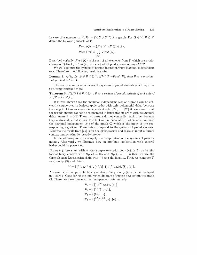
Attribute Exploration in a Fuzzy Setting 125
In case of a non-empty V , G := (V,E ∪ E−1) is a graph. For Q ∈ V , P ⊆ Vdefine the following subsets of V :
Pred (Q) := P ∈ V | (P,Q) ∈ E,P red (P) :=
⋃
Q∈PPred (Q).
Described verbally, Pred (Q) is the set of all elements from V which are prede-cessors of Q (in E). Pred (P) is the set of all predecessors of any Q ∈ P.
We will compute the systems of pseudo-intents through maximal independentsets. Therefore, the following result is useful:
Lemma 2. ([23]) Let ∅ 6= P ⊆ LM . If V \ P =Pred (P), then P is a maximalindependent set in G.
The next theorem characterises the systems of pseudo-intents of a fuzzy con-text using general hedges:
Theorem 5. ([23]) Let P ⊆ LM . P is a system of pseudo-intents if and only ifV \ P = Pred(P).
It is well-known that the maximal independent sets of a graph can be effi-ciently enumerated in lexicographic order with only polynomial delay betweenthe output of two successive independent sets ([24]). In [25] it was shown thatthe pseudo-intents cannot be enumerated in lexicographic order with polynomialdelay unless P = NP. These two results do not contradict each other becausethey address different issues. The first one in encountered when we enumeratethe maximal independent sets of the graph G which is the input of the cor-responding algorithm. These sets correspond to the systems of pseudo-intents.Whereas the result from [25] is for the globalisation and takes as input a formalcontext enumerating its pseudo-intents.
In the following we will exemplify the computation of the systems of pseudo-intents. Afterwards, we illustrate how an attribute exploration with generalhedge could be performed.
Example 4. We start with a very simple example. Let (g, a, b, I) be theformal fuzzy context with I(g, a) = 0.5 and I(g, b) = 0. Further, we use thethree-element Lukasiewicz chain with ∗ being the identity. First, we compute Vas given by (3) and obtain
V = 0.5/a,0.5 /b, 0.5/b, , 0.5/a, b, b, a.Afterwards, we compute the binary relation E as given by (4) which is displayedin Figure 6. Considering the undirected diagram of Figure 6 we obtain the graphG. There, we have four maximal independent sets, namely
P1 = , 0.5/a, b, a,P2 = 0.5/b, a,P3 = b, a,P4 = 0.5/a,0.5 /b, a.

126 C.V. Glodeanu
P1 and P3 do not satisfy the condition of Theorem 5 and are therefore not
0.5/a,0.5 /b
0.5/b
0.5/a, b
b a
Fig. 6. Binary relation E for (G,M, I)
systems of pseudo-intents. P2 and P4 do satisfy this condition and hence theyare systems of pseudo-intents yielding the stem bases displayed in Figure 7.
T2 T4
(1) 0.5/b ⇒ a (3) 0.5/a,0.5 /b ⇒ a(2) a ⇒0.5 /b (4) a ⇒0.5 /b
Fig. 7. Stem bases
Now we could start an attribute exploration, for instance in T2. The algorithmwould ask us:
Objects having attribute b to degree 0.5 also have attribute a to degree 1?
Let us answer this question affirmatively. The next question is:
Objects having attribute a to degree 1 also have attribute b to degree 0.5?
We deny this implication and provide a counterexample, namely the object hwith I(h, a) = 1 and I(h, b) = 0. This counterexample obviously respects thealready confirmed implication so the context is extended by the new object h.For this extended context we can compute the sets V and E. The binary relation

Attribute Exploration in a Fuzzy Setting 127
0.5/a,0.5 /b
0.5/b b 0.5/a, b
Fig. 8. Binary relation E for the extended context
E for the extended context is given in Figure 8. From this graph we obtain fourmaximal independent sets, three of which form systems of pseudo-intents. Thestem bases which they induce are displayed in Figure 9. At the beginning we
T p2 T pp
2 T ppp2
(5) 0.5/b ⇒ a (6) ⇒0.5 /a (8) b ⇒ a(7) 0.5/a, b ⇒ b
Fig. 9. Stem bases of the extended context
have confirmed implication (1) from Figure 7. However, this implication is nownot present any more in the stem bases T pp
2 and T ppp2 . This is also reflected in
the stem base T4. Even though the counterexample respects implication (3), thepseudo-intent belonging to this implication also disappears.
Concluding, by extending the context with objects which respect the alreadyconfirmed implications, the latter may disappear from the stem base of theextended context. Hence, we do not have an analogon of Proposition 2 for generalhedges.
The attribute exploration with general hedges raises a lot of questions andopen problems. First of all it is unclear whether such an exploration is desirable.We have more than one stem base for a context. These bases are equally pow-erful with respect to their expressiveness. The major problem however is howto perform an attribute exploration successfully. It is an open problem how toenumerate the pseudo-intents obtained by general hedges such that the alreadyconfirmed implication still remain in the stem base of the extended context. One
128 C.V. Glodeanu
could for instance make some constraints on the counterexamples. However, suchan approach is not in the spirit of attribute exploration.
5 Conclusion
We presented a generalisation of attribute exploration to the fuzzy setting. Theproblem is two-sided. If one uses the globalisation in the residuated lattice, thestem base is unique. For such a setting the results regarding the explorationfrom the crisp case can be transferred without problems and one can performsuccessfully an attribute exploration with attributes having fuzzy values. Us-ing hedges different from the globalisation one obtains more than one systemof pseudo-intents. This alone would not cause such a big problem. The majordifficulty comes with the fact that the already confirmed pseudo-intents are notnecessarily pseudo-intents of the extended context. This is therefore an openproblem, how to perform an attribute exploration using a general hedge.
In the future we will focus on the problem regarding the general hedge andon extensions of this method, as for instance on fuzzy attribute exploration withbackground knowledge. There, the user can enter in advance some implicationswhich he/she knows to hold between the attributes. Using such backgroundknowledge one usually has to provide less examples and answer to fewer ques-tions.
We are expecting that the method will have many practical applications, asits crisp variant has. Therefore, we will also focus on applications using attributeexploration in a fuzzy setting.
References
1. Ganter, B., Wille, R.: Formale Begriffsanalyse: Mathematische Grundlagen.Springer (1996)
2. Pollandt, S.: Fuzzy Begriffe. Springer Verlag, Berlin Heidelberg New York (1997)3. Belohlavek, R.: Fuzzy Relational Systems: Foundations and Principles. Volume 20
of IFSR Int. Series on Systems Science and Engineering. Kluwer Academic/PlenumPress (2002)
4. Belohlavek, R., Vychodil, V.: Attribute implications in a fuzzy setting. In: ICFCA.(2006) 45–60
5. Belohlavek, R., Chlupova, M., Vychodil, V.: Implications from data with fuzzyattributes. In: AISTA 2004 in Cooperation with the IEEE Computer SocietyProceedings. (2004)
6. Guigues, J.L., Duquenne, V.: Familles minimales d’implications informatives re-sultant d’un tableau de donnes binaires. Math. Sci. Humaines 24(95) (1986) 5–18
7. Sacarea, C.: Towards a theory of contextual topology. PhD thesis, TH Darmstadt,Aachen (2001)
8. Kwuida, L., Pech, C., Reppe, H.: Generalizations of boolean algebras. an attributeexploration. Math. Slovaca 56(2) (2006) 145–165
9. Revenko, A., Kuznetsov, S.: Attribute exploration of properties of functions onordered sets. In: Proc. CLA 2010. (2010) 313–324

Attribute Exploration in a Fuzzy Setting 129
10. Eschenfelder, D., Kollewe, W., Skorsky, M., Wille, R.: Ein Erkundungssystem zumBaurecht: Methoden der Entwicklung eines TOSCANA-Systems. Volume 2036.Techn. Univ., FB 4, Darmstadt (Januar 1999) Ersch. ebenf. in: Begriffliche Wis-sensverarbeitung: Methoden und Anwendungen. Hrsg.: G. Stumme, R. Wille. -Berlin, Heidelberg (u.a.): Springer, 2000. S. 254-272.
11. Bartel, H.G., Nofz, M.: Exploration of nmr data of glasses by means of formalconcept analysis. Chemom. Intell. Lab. Syst. 36 (1997) 53–63
12. Stumme, G.: Acquiring expert knowledge for the design of conceptual informationsystems. In Fensel, D., Studer, R., eds.: EKAW. Volume 1621 of Lecture Notes inComputer Science., Springer (1999) 275–290
13. Ganter, B.: Attribute exploration with background knowledge. Theor. Comput.Sci. 217(2) (1999) 215–233
14. Stumme, G.: Attribute exploration with background implications and exceptions.In Bock, H.H., Polasek, W., eds.: Data Analysis and Information Systems. Sta-tistical and Conceptual approaches. Proc. GfKl’95. Studies in Classification, DataAnalysis, and Knowledge Organization 7, Heidelberg, Springer (1996) 457–469
15. Wille, R.: Bedeutungen von Begriffsverbanden. In Ganter, B., Wille, R., Wolff,K.E., eds.: Beitrage zur Begriffsanalyse. B.I.–Wissenschaftsverlag, Mannheim(1987) 161–211
16. Zickwolff, M.: Rule exploration: first order logic in formal concept analysis. Tech-nische Hochschule Darmstadt. (1991)
17. Hajek, P.: The Metamathematics of Fuzzy Logic. Kluwer (1998)18. Hajek, P.: On very true. Fuzzy Sets and Systems 124(3) (2001) 329–33319. Belohlavek, R., Funiokova, T., Vychodil, V.: Galois connections with hedges. In
Liu, Y., Chen, G., Ying, M., eds.: Eleventh International Fuzzy Systems Associa-tion World Congress,. Fuzzy Logic, Soft Computing & Computational Intelligence,Tsinghua University Press and Springer (2005) 1250–1255
20. Belohlavek, R., Vychodil, V.: Fuzzy concept lattices constrained by hedges. JACIII11(6) (2007) 536–545
21. Belohlavek, R.: Algorithms for fuzzy concept lattices. In: Proc. Fourth Int. Conf.on Recent Advances in Soft Computing. (2002) 200–205
22. Belohlavek, R., Vychodil, V.: Fuzzy attribute logic: attribute implications, theirvalidity, entailment, and non-redundant basis. In Liu, Y., Chen, G., Ying, M., eds.:Eleventh International Fuzzy Systems Association World Congress,. Volume 1 ofFuzzy Logic, Soft Computing & Computational Intelligence., Tsinghua UniversityPress and Springer (2005) 622–627
23. Belohlavek, R., Vychodil, V.: Fuzzy attribute implications: Computing non-redundant bases using maximal independent sets. In: Australian Conference onArtificial Intelligence. (2005) 1126–1129
24. Johnson, D.S., Yannakakis, M., Papadimitriou, C.H.: On generating all maximalindependent sets. Information Processing Letters 27(3) (1988) 119–123
25. Distel, F., Sertkaya, B.: On the complexity of enumerating pseudo-intents. DiscreteApplied Mathematics 159(6) (2011) 450–466

On Open Problem - Semantics of the CloneItems
Juraj Macko
Dept. Computer SciencePalacky University, Olomouc
17. listopadu 12, CZ-77146 OlomoucCzech Republic
email: [email protected]
Abstract. There was presented a list of open problems in the FormalConcept Analysis area at the conference ICFCA 2006. The problem num-ber seven deals with the semantics of the clone items. Namely, for whomcan clone items make sense and for whom can make sense the item,which can cause, that clones disappear in the collection of itemsets. Inthis paper we propose the semantics behind clone items with the coupleof examples. Definition of the clone items is very strict and theirs usecould be very limited in the real datasets. We introduce method, how todeal with items, which properties are very near to the clones. We alsohave a look on the items, which causes the disappearing of the clones, ordecrease (increase) the degree of property ”to be clone”. In the experi-ment part we analyze some known datasets from the clone items point ofview. The results bring a couple of new questions for the future research.
Keywords: formal concept analysis, clone items
1 Introduction
This paper is structured as follows: The first part, which is actually cited fromthe source, where the problem were defined [2] describes and defines the wholeproblem - the semantics of the clone items. In the second part is proposed thesemantics of the clone items by putting the problem into the other point ofview. There is also a discussion here, about another possible definitions of theclones as presented in [1]. In this part three comprehensive examples can befound. The third part tries to set a quite new approach to the clone items.The attributes, which are not clones, but they have properties very close toclones are considered. A nearly clones are defined. In this part some results fromthe introductory experiments about the clones and nearly clones are presented.Finally, the conclusion is divided in two parts - conclusion of defined problemand conclusion of other proposed issues.

On Open Problem - Semantics of the Clone Items 131
2 The Problem Setting
The proposed problem of the semantics of the clone items were proposed anddefined in [2] as follows: Let J be a set of items x1, ..., x|J|, let F be a collectionof subsets of J and let ϕa,b be the mapping ϕa,b : 2J → 2J defined by followingformula:
X → ϕa,b(X) =
(X\a) ∪ b if b /∈ X and a ∈ X(X\b) ∪ a if a /∈ X and b ∈ XX elsewhere
It means swapping items a and b, which are called clone items in F iff for anyF ∈ F , we have ϕa,b(F ) ∈ F . A Clone-free collection is, if it does not containany clone items.
Let (X,Y, I) be a formal context such that attributes a ∈ Y and b ∈ Y arenot clones. Consider the formal sub-context (X,Z, I), where Z ⊂ Y , such that aand b are clone in (X,Z, I). Let c ∈ Y \Z such that a and b are no longer clonein (X,Z ∪ c, I). Attributes a and b has symmetrical behaviour in (X,Z, I),but this behaviour is lost when we add the attribute c to the formal context.The following question are asked:
1. Does such symmetrical behaviour of a and b make sense for someone?2. Does it make the sense, that such symmetrical behaviour disappears, when
the attribute c is added?3. What is semantics behind the attributes a, b, and c?
3 Semantics behind Clones
3.1 Semantics behind Clones - Auxiliary Formal Definitions
The collection of itemsets will be defined as a formal context (X,Y, I), where Xis a set of objects and Y is a set of attributes. Objects and attributes are relatedby I ⊆ X×Y , which means, that the object x ∈ X has the attribute y ∈ Y . ForA ⊆ X, B ⊆ Y and formal context (X,Y, I) we define operators
A↑I = y ∈ Y | for each x ∈ X : 〈x, y〉 ∈ IB↓I = x ∈ X | for each y ∈ Y : 〈x, y〉 ∈ I
The two given attributes a, b ∈ Y will be investigated, whether are clones or not.For this purpose the pivot table will be defined as the relation R ⊆ P × N ,where P = a, b ⊆ Y and N is a set of all Nj , where j ∈ [1; |N |]. Nj ∈ Nrepresents the set of attributes Nj = x↑I ∩ (Y \P ) for each x ∈ X such thata, b ∩ x↑I 6= ∅ and a, b * x↑I . The investigated attributes a, b ∈ P ⊆ Ywill be named the pivot attributes and all other considered attributes, hence
n ∈ ⋃|N |j=1Nj , we denote as the non-pivot attributes. Nj is a set generated
by pivot attributes (or shortly the generated set). The pivot table has two

132 J. Macko
rows. The ”cross” × in pivot table will represent the fact, that in the formalcontext there exists at least one row, where the investigated attribute a (or brespectively) appears together with the attributes in the particular Nj . Formally,
〈a,Nj〉 ∈ R iff in context (X,Y, I) exists x ∈ X such that x↑I = a ∪Nj ,
〈b,Nj〉 ∈ R iff in context (X,Y, I) exists x ∈ X such that x↑I = b ∪Nj .
Based on pivot attributes, non-pivot attributes and formal context (X,Y, I)consider pivot table which is as new formal context (P,N , R) with operatorsfor C ⊆ P and D ⊆ N defined as follows
C↑R = Ni ∈ N | for each p ∈ P : 〈p,Nj〉 ∈ R,D↓R = p ∈ P | for each Ni ∈ N : 〈p,Nj〉 ∈ R
In the pivot table (P,N , R) we are trying to find whether a↑R = b↑R . In
a b n1 n2 n3
x1 × × ×x2 × × ×x3 × × ×x4 × × ×x5 × × ×x6 × × ×x7 × × × ×x8 × × × ×
N1
=n
1,n
2
N2
=n
2,n
3
N3
=n
1,n
3
N4
=n
1,n
2,n
3
a × × × ×b × × × ×
a b n1 n2 n3 c
x1 × × × ×x2 × × × ×x3 × × ×x4 × × ×x5 × × × ×x6 × × ×x7 × × × ×x8 × × × × ×
N1
=n
1,n
2,c
N2
=n
2,n
3
N3
=n
1,n
3
N4
=n
1,n
3,c
N5
=n
1,n
2,n
3
N6
=n
1,n
2,n
3,c
a × × × ×b × × × ×
(i) Formal context (ii) Pivot table (iii) Formal context (iv) Pivot table(X,Z, I) (P,N , R) (X,Z ∪ c, Ic) (P,Nc, Rc)
Fig. 1. Formal context and pivot tables with and without clones
other words, we want to know, whether the attribute a appears in given formalcontext with the same combination of other attributes, as b appears (in the sameformal context). If yes, the pivot attributes a, b in context (X,Y, I) generates thesame generated sets. In other words, a, b are not unique with respect to the non-pivot attributes. Such attributes we call clones. When a↑R 6= b↑R , attributesa, b are unique with respect to the non-pivot attributes, because generates at leastone different generated set. The attribute c ∈ Y , which makes a, b unique withrespect to generated sets is called the originality factor of a, b. In Figure 1 weshow examples of the contexts and pivot tables with clones or with the originalityfactor respectively. By introducing the pivot table, the whole problem have beenput to the other point of view. The proposed semantics will be explained basedon the previous definitions.

On Open Problem - Semantics of the Clone Items 133
3.2 Discussion and Remarks
Before the comprehensive examples will be proposed, it is necessary to discussprevious auxiliary definition of the clones using the pivot table. There are coupleof problems mainly dealing with ambiguity of the pivot table definition withrespect to the various definitions of the clones used by the several authors inthe other works. In the pivot table definition the set Nj ∈ N is defined asNj = x↑I ∩ (Y \P ) for each x ∈ X such that
1. a, b ∩ x↑I 6= ∅ and2. a, b * x↑I .
The first condition tells, that we ignore the itemsets (rows), where neither anor b is present. Such items are not interesting when we investigate whethe a andb are clones, so we will ignore them when the pivot table is defined. The secondcondition excludes itemsets, where we have the both pivot attributes a and band the question is: Why we exclude such itemsets from pivot table, when wecan see it in original definition of the clone items? Recall the original definitionof the clones:
X → ϕa,b(X) =
(X\a) ∪ b if b /∈ X and a ∈ X(X\b) ∪ a if a /∈ X and b ∈ XX elsewhere
Items a and b, which are called clone items in F iff for any F ∈ F , we haveϕa,b(F ) ∈ F . So we need to have the original itemset and swapped itemset aswell in the whole collection of itemsets. In definition of ϕ are interesting therows 1 and 2. The row 3 is only technical condition. It means, that fulfillmentof swapping condition of itemsets, which does not contain any of a or b or con-versely, when it contains both, is trivial. So we could add them in the pivottable by skipping the condition a, b * x↑I , but we consider such informa-tion redundant and hence useless. However, the semantics of the clones remainsunchanged. But on the other side, it can influence the value of the degree ofclones dI(a,b) (which will be defined later). In such case we need to investigate,which definition would be more precise for the user. The basic idea of our se-mantics of clones (and nearly clones defined later as well) is, of how original areitems a and b in the whole collection of itemsets. The itemsets which does notinclude either a or b will not tell us anything about originality of such items, theitemsets which include both as well.
The other point for the discussion comes from the problem number six (pre-sented in [2]), which deals with the size of a clone-free Guigues-Duquenne basis.Namely, whether the clone items are responsible for the combinatorial explo-sion of some Guigues-Duquennes basis. The Guigues-Duquennes basis is non-redundant. All other attribute implications, which holds in given context, canbe derived from this base. In the paper [1] there are presented some partial re-sults, which includes definitions and propositions dealing with the clones. The

134 J. Macko
clones are defined with respect to pseudo-closed sets in the collection of theclosed itemsets. The one of the basic results is, that in order to detect cloneitems, one has to consider meet-irreducible itemsets only (for details see [1]).The definition of the clone items given in [2] is defined in more general manner.It is based not only on the pseudo-closed itemset collection, but it is defined forarbitrary collection of itemsets. This fact can cause, that two items may not ap-pear as clone according the definition in [2], but the are still clones in definitionaccording to [1]. In the rest of the paper there will be considered the definitionused in [2] only. However, the proposed semantics would be slightly modified,when we would need to use it in the meaning of [1].
The other important part is to compare proposed solution with other at-tempts or solutions, but the author has no information either about such at-tempts or about some real solutions. Hence, according to the author’s bestknowledge, the author’s proposed solution seems to be novel.
3.3 Semantics behind Clones - Examples
In this part we would like to show on couple of examples, how the clone itemsand the originality factor can be used. The originality factor can be desired undersome conditions, but undesired under the other conditions. Inall examples thesame formal context and the pivot tables will be used, but always with the dif-ferent meaning of the objects and attributes. The Table 1 represents the originalformal context (X,Z, I) with the clones a and b and it also represents the formalcontext (X,Z ∪ c), where the originality factor c is added. The correspondingpivot tables (P,N , R) and (P,Nc, Rc) can be seen in the Table 2. A labeling ofthe objects and the pivot attributes is done according to the particular sets Xand Y defined in each example below.
The sales analysis Let X = Customer1, . . . , Customer8 be a set of cus-tomers and the set of attributes is defined as Y = Man,Woman, n1, n2, n3, c.The attributesMan andWoman represents the sex of customer and the other at-tributes represents the products bought by each customer. The following formalcontexts represents a marketing research of the sales company (the customers andtheirs attributes). In the formal context (X,Z, I) attributes Man and Womanare clones. In the pivot table (P,N , R) attributes Man and Woman are pivotattributes and nj is product bought by customer. On the other hand, in theformal context (X,Z ∪ c) and the corresponding pivot table (P,Nc, Rc) theattributes Man and Woman are no longer clones and the attribute c (Productc) is the originality factor in this case. Namely, for the itemset Man, n1, n3, cthere is no corresponding itemset Woman, n1, n3, c.
How can this information be used for the marketing department? Imagine,that the sales company wants to create packages based on the marketing re-search. These packages should consist of the particular products nj . In the first

On Open Problem - Semantics of the Clone Items 135
Man
/Europe
/Gene1
Wom
an
/America
/Gene2
n1 n2 n3 c
Customer 1 / Animal 1 / Organism 1 × × × ×Customer 2 / Animal 2 / Organism 2 × × × ×Customer 3 / Animal 3 / Organism 3 × × ×Customer 4 / Animal 4 / Organism 4 × × ×Customer 5 / Animal 5 / Organism 5 × × × ×Customer 6 / Animal 6 / Organism 6 × × ×Customer 7 / Animal 7 / Organism 7 × × × ×Customer 8 / Animal 8 / Organism 8 × × × × ×Table 1. Formal contexts (X,Z, I) and (X,Z ∪ c, Ic)
N Nc
N1
=n
1,n
2
N2
=n
2,n
3
N3
=n
1,n
3
N4
=n
1,n
2,n
3
N1
=n
1,n
2,c
N2
=n
2,n
3
N3
=n
1,n
3
N4
=n
1,n
3,c
N5
=n
1,n
2,n
3
N6
=n
1,n
2,n
3,c
Man / Europe / Gene1 × × × × × × × ×Woman / America / Gene2 × × × × × × × ×
Table 2. Pivot tables (P,N , R) and (P,Nc, Rc)

136 J. Macko
case of the formal context (X,Z, I) the company can create the same packagesfor man and for woman, because male and female customers buy the same com-binations of products nj . The same packages for two different groups can reducethe total cost of production, because we need to produce only four types of thepackages, namely the packages N1 = n1, n2, N2 = n2, n3, N3 = n1, n3 andN4 = n1, n2, n3. With the attribute c added to the formal context, we need sixdifferent packages, because only the packages N1 = n1, n2 and N2 = n2, n3can be produced for men and women at the same time. Other packages are dif-ferent for the male and female customers. From this point of view, the originalityfactor is undesired and the clones are desired.
But we can use this information in the other way. Suppose, that the costdifference of producing four or six package types is not significant, but significantcan be a targeted marketing on the male and female customers. The formalcontext (X,Z, I), where we have the clone attributes Man and Woman, doesnot provide differentiated information about the male and female customers. Onthe other hand, the formal context (X,Z ∪ c) does. The attribute c providesdesired information, that the Product c influences the different combinationof the products bought by the male and female customer. It means, that wecan make targeted marketing (namely, the different type of packages for thedifferent type of customers) based on the originality factor Product c and itscombinations with the other products. Some combinations of the products withthe originality factor can be used as a topic for advertising to highlight thedifference between man and woman preferences. However, the clone analysis canprovide the marketing department with the useful information in both cases.
Analysis of the animals Let X = Animal1, . . . , Animal8 be a set of ani-mals and a set of attributes is defined as Y = Europe,America, n1, n2, n3, c.The formal context (X,Z, I) in the Table 1, shows the attributes Europe andAmerica as clones. This fact can be interpreted as follows: In Europe and inAmerica they live the same types of animals, when we consider the attributes ofthe animals n1, n2 and n3 only. The same information can be seen in the pivottable Table 2. When we add the attribute c, we can see the different types ofanimals (with the different generated sets) in Europe and in America as well(see Table 2). The information, that exists the originality factor c for attributesEurope and America can be interpreted as follows: It shows, that Europe andAmerica are somehow specific. In Europe are some different combinations ofanimal’s attributes than in America and vice versa and at the same time we see,that this difference somehow deals with the attribute c. Biologist can investi-gate in more details, what is specific in Europe and in America, which specificattribute of Europe leads to the different attributes of the animals in Europe(and vice versa). Other use of such information is following: From a backgroundknowledge we know, that there is no reason for differentiating the animals in Eu-rope and America just on attribute c. In our dataset we do not have in Americathe animal with attributes n1, n3 and c, but with respect to the attribute c we

On Open Problem - Semantics of the Clone Items 137
expect to have the same types of animals in Europe and in America. Thus, weneed to look for such animal in America as well. Our hypothesis is, that in Amer-ica lives such animal, because it lives in Europe and based on our backgroundknowledge there is no reason for c to be the originality factor. From the formalpoint of view, we do not have the complete dataset (formal context). Some rowsare missing, and we need to find such objects in the reality (in this case we arelooking for the animal).
Analysis of genes and the morphological attributes of organisms Thelast example use set X = Organism1, . . . , Organism8 and set of attributesY = Gene1, Gene2, n1, n2, n3, c The attributes Gene1 and Gene2 are clonesin formal context (X,Z, I) in Table 1 and the other attributes represents themorphological property of the organism. The interpretation can be following:Organisms with Gene1 and Gene2 has the same combination of morphologicalproperties Nj , when we consider the morphological properties of organisms n1,n2 and n3. The same information can be seen in the pivot table Table 2. When weadd the morphological attribute c, we get the formal context (X,Z∪c), whichmeans, that based on attribute c there are some different types of the morpho-logical attributes of organisms with the Gene1 and Gene2 (see the Table 1 andTable 2). It shows, that the Gene1 and Gene2 probably does not influence thesets of the morphological attributes containing only n1, n2, n3, but this Gene1and Gene2 influence the sets of the morphological attributes containing c. Thus,c as the originality factor makes the difference between these two genes. Thisinformation could be useful for a hypothesis creation in genetics.
4 Nearly Clones
4.1 Degree of Clones and Degree of Originality
The definition of the clone items is very strict. Recall, that condition ϕa,b(F ) ∈ Fneeds to be true for any F ∈ F . We can see, that adding only one ”cross” intothe huge formal context can cause, that two clones disappear. We expect, thatin real dataset such condition can be true very rarely. When we want to usethe clone items meaningfully, we need to have a weaker definition. For practicalpurposes it suffices, that condition ϕa,b(F ) ∈ F can be true in some reasonableamount of F ∈ F . We define degree of clone as
dI(a,b) =|a↑R ∩ b↑R ||a↑R ∪ b↑R | ,
which can be read as follows: The attributes a and b with respect to the formalcontext I are clones in the degree d. For a priori given threshold θ we define aand b as nearly clones iff d(a,b) ≥ θ. Note, that for d(a,b) = 1 the attributes aand b are clones and for d(a,b) = 0 we say, that they are original attributes.Consider now the formal context (X,Z, IZ) and the corresponding pivot table(P,NZ , RZ) (see Figure 2). We can see, that a and b are clones with the degree

138 J. Macko
dIZ(a,b) = 1. Adding either attribute c1 or attribute c2 to the formal context leads
to decreasing of clone degree for a and b. Namely, dIc1(a,b) = 0 and d
Ic2(a,b) = 0, 6. In
both cases degree has decreased, but the resulted clone degree is different. In thefirst case attributes are original, in the second case attributes are nearly clonesfor arbitrary θ ≤ 0, 6. Such situation can be formalized, and define the degreeof originality for given ci and context (X,Z, I) as
gIc(a,b) = dI(a,b) − dIc(a,b)The degree of originality shows, how the attribute, added to the context,
does influence the degree of clone for given attributes a, b ∈ Y and the formalcontext (X,Z, I).
a b n1 n2 n3 c1 c2
x1 × × × × ×x2 × × ×x3 × × × ×x4 × × ×x5 × × × ×x6 × × ×x7 × × × × ×x8 × × × ×
N1
=n
1,n
2
N2
=n
2,n
3
N3
=n
1,n
3
N4
=n
1,n
2,n
3
a × × × ×b × × × ×
N1
=n
1,n
2,c
1
N2
=n
1,n
2
N3
=n
2,n
3,c
1
N4
=n
2,n
3
N5
=n
1,n
3,c
1
N6
=n
1,n
3
N7
=n
1,n
2,n
3
N8
=n
1,n
2,n
3,c
1
a × × × ×b × × × ×
N1
=n
1,n
2,c
2
N2
=n
1,n
2
N3
=n
2,n
3
N4
=n
1,n
3
N5
=n
1,n
2,n
3
a × × × ×b × × × ×
(i) Formal contexts (ii) Pivot table (iii) Pivot table (iv) Pivot table(X,Z, IZ), (P,NZ , RZ) (P,Nc1 , Rc1) (P,Nc2 , Rc2)
(X,Z ∪ c1, Ic1), from context from context from contextand (X,Z, IZ) (X,Z ∪ c1, Ic1) (X,Z ∪ c2, Ic2)
(X,Z ∪ c2, Ic2) dIZ(a,b) = 1 dIc1(a,b) = 0 d
Ic2(a,b) = 0, 6
Fig. 2. Formal contexts and pivot tables with different degrees of clone.
4.2 Experiment Nr. 1 - Amounts and Degrees of Nearly Clones inDatasets
For the purpose of this paper we arranged two introductory experiments with thenearly clones, in which we use datasets Mushroom [3], Adults [4] and Anonymous[5] from well known UC Irvine Machine Learning Repository (for the detailssee Table 3). In the experiments we used a naive algorithm (the brute-forcesearch, but with polynomial complexity) for finding the degrees of clones asdefined above. Looking for more efficient algorithm is out of scope of this paper.The algorithm was implemented in C, and all experiments have been run onthe computer with an Intel Core i5 CPU, 2.54 Ghz, 6 GB RAM, 64bit W7Professional.

On Open Problem - Semantics of the Clone Items 139
In the first experiment we were focused on finding all nearly clone pairs, withd(a,b) > 0, especially we investigated, if there are some clones (where d(a,b) = 1)in the real datasets. The results of the first experiment are shown in Table 3.
Mushroom [3] Adults [4] Anonymous [5]
Number of objects 8 124 48 842 32 713Number of attributes 119 104 295Number of nearly clones d(a,b) > 0 113 1 568 382Maximal d(a,b) > 0 1,00000 0,02252 0,00187Minimal d(a,b) > 0 0,00123 0,00014 0,00143Average d(a,b) > 0 0,24423 0,00449 0,00160Median d(a,b) > 0 0,14537 0,00195 0,00159Slope 0,99402 0,77895 0,55004
Table 3. Overview of the datasets and results of the first experiment (source ofdatasets: http://archive.ics.uci.edu/ml/index.html)
(i) nearly clone pairs for d(a,b) > θ = 0 (ii) nearly clone pairs for d(a,b) ≥ θ = 0.5x-axis - number of nearly clone pairs x-axis - number of nearly clone pairs
y-axis - degree of clone d(a,b) y-axis - degree of clone d(a,b)z-axis - number of objects processed z-axis - number of objects processed
Fig. 3. Mushroom - distribution of d(a,b) in dataset scaled by 1000 objects.
In case of the dataset Mushroom, we present also the distribution of the clonedegrees and some other details as well. Figure 3 shows the volume of all pairsa and b and clone degree d(a,b) > 0, for each scale pattern (from 1000 to 8124by 1000). In (i) are displayed all pairs with d(a,b) > 0 and part (ii) is morefocused on the amount of pairs where d(a,b) ≥ 0, 5 for each investigated scaledpattern. Note, that the results from numbers of the processed objects in thedataset Mushroom (namely from 1000 to 7000 depicted in z-axis in the Figure3) depends on an order of the processing objects. This fact were not investigated

140 J. Macko
more deeply. However, when we have processed all 8124 objects, the order willnot influence the result. Figure 4 shows some interesting details. In (i) there arepresented the pairs a, b with d(a,b) = 1, in (ii) the same for 1 > d(a,b) ≥ 0, 5 . Wehave found 4 clone pairs, and one clone triple. In the clone triple (103, 104, 105)we can see the transitivity (i.e. when (a, b) are clones and b, c are clones, also aand c are clones). Such transitivity is not surprising and is direct consequenceof the clone definition.
What does such results show and does it appear reasonable? The Figure 4part (i) shows the clones a and b. The original dataset Mushroom consists of 22attributes with non-binary values. For the purposes of clone investigation, thisdataset were nominally scaled to the formal context, which is binary indeed. Itis interesting to see, that all clone items represents the value of the same originalattribute. E.g. clones 019 and 021 represents the original attribute Cap Color,thus its values Purple or White respectively. Another example is clone triple 103,104 and 105 which represents the original attribute Spore Print Color with thecorresponding values Orange, Purple and White. It can be interpreted as fol-lows: Purple and white color generates the same sets of the non-pivot attributes.In other words, to each mushroom with the purple cap (the pivot attribute),there exists corresponding mushroom with the white cap (the pivot attribute),but all other properties remains he same (non-pivot attributes). Similarly to eachmushroom with the purple spore print color, there exists corresponding mush-room with the white spore print color and the corresponding mushroom with theorange one. When we look on the nearly clones in the Figure 4 part (ii), the at-tributes 69 and 70 represents the same original attribute stalk color above ringwith the values cinnamon and gray (the details are not shown in the table).These attributes are not the clones, but the nearly clones with the clone degreed(a,b) = 0, 96. It can be interpreted similarly as by the clones. Only the differencewill be in a quantifier. By clones the quantifier was ”for each”, by the nearlyclones we will have fuzzy quantifier, in this case ”for the most”. Hence the inter-pretation is: For the most mushroom with cinnamon stalk above the ring existscorresponding mushroom with the corresponding gray stalk above the ring (andvice versa). The clone degree is very high in this case (d(a,b) = 0, 96) it meansthere are only couple of mushrooms with cinnamon stalk above the ring color,which do not have corresponding mushroom with the gray stalk above the ringcolor. However, the for the deeper understanding of such examples, it is requiredto ask an expert in mycology.
4.3 Experiment 2 - Structure of Nearly Clones in Datasets
In the second experiment we investigated the structure of nearly clones. Namely,we have defined a fuzzy relation T : Y × Y → L, where L = [0; 1] is defined asT (a, b) = d(a,b) ∈ L. In other words, the fuzzy relation express the degree of theclone for each pair a, b ∈ Y . For the better visualization we display such relationin so called ”bubble chart”. The bubble chart displays three dimensional datain two dimensional chart. The position of the bubble is given by two dimensions

On Open Problem - Semantics of the Clone Items 141
(x and y axis) and the size of the bubble shows the third dimension. The resultsfrom the first experiments are displayed in bubble chart, where the pairs ofattributes a and b represents two dimensions and the degree of clone d(a,b) isrepresented by the size of the bubble. Note, that the fuzzy relation T is indeedsymmetric (i.e. d(a,b) = d(b,a)), but we show only part of the relation, wherea < b. Figures 5, 6 and 7 show the structure of the nearly clones for the datasetsMushroom, Anonymous and Adults. We can observe very different structure ofthe nearly clones in each dataset. In Mushroom we can see, that the structureof the nearly clones is approximately linear. All nearly clones are clustered nearto the line defined as (y, y). In the case of Adults dataset we can see morespread, but still approximately linear structure, except of one cluster near point(0, |Y |). The nearly clones of the data set Anonymous forms the different, butkind of regular structure as well. This results leads to the question, what kind ofproperties has fuzzy relation of the nearly clones and if properties of such fuzzyrelation correlates with the properties of the formal context, or with propertiesof the concept lattice. Until now we know, that such relation is transitive forclone items d(a,b) = 1 and symmetric for the arbitrary nearly clone items, butthis two properties are trivial. I would be also interesting to find the semanticsof such fuzzy relation defined on the nearly clones. All this will be part of thefuture investigation.
original attributes a b d(a,b) = 1
03. cap-color 019 purple=u 021 white=w 1,0005. odor 025 almond=a 026 anise=l 1,0005. odor 030 musty=m 031 none=n 1,0017. veil-color 086 brown=n 087 orange=o 1,0020. spore-print-color 103 orange=o 104 purple=u 1,0020. spore-print-color 103 orange=o 105 white=w 1,0020. spore-print-color 104 purple=u 105 white=w 1,00
a b d(a,b) ≥ 0.5
69 70 0,9697 98 0,9578 79 0,842 5 0,8449 50 0,7412 16 0,6640 42 0,51
(i) Clones (ii) Nearly clones
Fig. 4. Dataset Mushroom - experiment on nearly clones
5 Conclusion and Future Perspectives
The paper was motivated by open problem proposed at ICFCA 2006 [2]. Wehope, that this small open problem is solved now and the reason is presentedin the first part of the conclusion. This part is structured as a direct answerson proposed questions. The second part of the conclusion describes ideas, whichoverlaps the original open problem and come with some new questions.
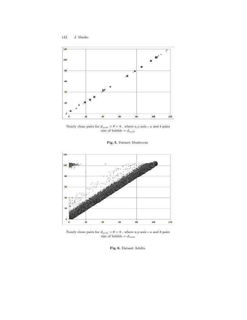
142 J. Macko
Nearly clone pairs for d(a,b) > θ = 0 , where x,y-axis - a and b pairssize of bubble = d(a,b)
Fig. 5. Dataset Mushroom
Nearly clone pairs for d(a,b) > θ = 0 , where x,y-axis - a and b pairssize of bubble = d(a,b)
Fig. 6. Dataset Adults

On Open Problem - Semantics of the Clone Items 143
Nearly clone pairs for d(a,b) > θ = 0 , where x,y-axis - a and b pairssize of bubble = d(a,b)
Fig. 7. Dataset Anonymous
5.1 Conclusion for Open Problem Questions
Question 1: Does the symmetrical behaviour of a and bmake sense for someone?Answer 1: Yes, such symmetrical behaviour can identify the same combinationof the non-pivot attributes with respect to pivot attributes and can make sense:
– for the marketing department to reduce cost of packages - the clone itemsenable the same packages for the different types of customers (e.g. man andwoman)
– for biologists to complete the the dataset - the clone items are expected, be-cause the originality factor c, has no sense based on the background knowl-edge. Hence, we some miss rows in the dataset (e.g. we need to find the newanimals)
– for genetics - it bring an information that the two genes has no influence ona combination of the morphological properties of organisms
– generally for everyone, who needs an information about the same combina-tion of non-pivot attributes with respect to the pivot attributes
Question 2: Does it make sense, that such symmetrical behaviour disappear,when c is added?Answer 2: Yes, such attribute is called the originality factor for the items aand b and can be useful:

144 J. Macko
– for the marketing department to make a targeted marketing for the differenttypes of customers (e.g. man and woman) using unique combination of thenon-pivot attributes
– for biologist to find the difference between two pivot attributes (e.g. Europeand America) with respect to other non-pivot properties. The originalityfactor c reveals, that the pivot attributes are original and this originalityneeds to be investigated deeper.
– for genetics - it brings an information, that two genes has an influence on acombination of the morphological properties of organisms
– generally for everyone, who needs an information about the reason, why thenon-pivot attributes has the different combinations with respect to the pivotattributes.
Question 3: What is semantics behind a, b, and c?Answer 3: The attributes a and b are the pivot attributes, all other attributesare the non-pivot attributes and c is moreover the originality factor for theattributes a and b. The pivot attributes generates a combination of the non-pivot attributes in the given context. The attribute c make the attributes a andb unique, which can be ”good” or ”bad”. It depends on a goal of the analysis.
5.2 Conclusion and Future Perspectives
The second part of conclusion shows, that the clones are very strictly defined.Therefore the nearly clones were introduced. The nearly clones operates withthe degree, in which two attributes are clones. Such formalization asks itself forstudy of the nearly clones under fuzzy setting (e.g. we have already mentioned,that structure of nearly clones can be seen as fuzzy relation indeed). The intro-ductory experiments shows, that the nearly clones in dataset have an interestingstructure, which needs to be investigated more deeply. This paper was introduc-tory for the nearly clones. As a future work we plan to describe more efficientalgorithm to compute the nearly clones for the given threshold θ, and algorithmfor identifying the originality factors for another given threshold ω. Finally wehope, that this paper, even it does not come with a great mathematical or ex-perimental results, brings some interesting ideas to FCA community.
Acknowledgements. The author is very grateful to the reviewers for theirhelpful comments and suggestions. Partly supported by IGA (Internal GrantAgency) of the Palacky University, Olomouc is acknowledged.
References
1. Gely A,, Medina A., Nourine L. and Renaud Y.: Uncovering and Reducing HiddenCombinatorics in Guigues-Duquenne Bases. Springer, Lecture Notes in ComputerScience, 2005, Volume 3403/2005, 235-248, Heidelberg 2005
2. more authors: Some open problems in Formal Concept Analysis. ICFCA 2006, Dres-den, http://www.upriss.org.uk/fca/fcaopenproblems.html

On Open Problem - Semantics of the Clone Items 145
3. Schlimmer,J.S. : Concept Acquisition Through Representational, Adjustment (Tech-nical Report 87-19). (1987). Doctoral disseration, Department of Information andComputer Science, University of California, Irvine.
4. Kohavi R.: Scaling Up the Accuracy of Naive-Bayes Classifiers: a Decision-TreeHybrid Proceedings of the Second International Conference on Knowledge Discoveryand Data Mining, 1996
5. Breese J., Heckerman D., Kadie C.: Empirical Analysis of Predictive Algorithms forCollaborative Filtering. Proceedings of the Fourteenth Conference on Uncertaintyin Artificial Intelligence, Madison, WI, July, 1998.

Computing the Skyline of a Relational TableBased on a Query Lattice
Nicolas Spyratos, Tsuyoshi Sugibuchi, Ekaterina Simonenko, and CarloMeghini
Laboratoire de Recherche en Informatique, Universite Paris-Sud 11, FranceNicolas.Spyratos, Tsuyoshi.Sugibuchi, [email protected]
Istituto di Scienza e Tecnologie della Informazione del CNR, Pisa, [email protected]
Abstract. We propose a novel approach to computing the skyline setof a relational table R, with respect to preferences expressed over oneor more numerical attributes. Our approach is based on what we callthe query lattice of R, and our basic algorithm constructs the skylineset as the union of the answers to a subset of queries from that lattice -hence without directly accessing the table R. Therefore, in contrast to allexisting techniques, our approach is independent of how the table R isimplemented or how its tuples are indexed. We demonstrate the general-ity of our approach by computing the skyline set of the join of two tablesbased on the product of their individual query lattices - therefore withoutperforming the join. The paper presents basic concepts and algorithmsleaving experimentation and performance evaluation to a forthcomingpaper.
Keywords: skyline, relational table, query lattice
1 Introduction
In many multicriteria decision-making applications, dominance analysis is an im-portant aspect. As an example, consider a person looking for a vacation packageusing two criteria, or “attributes”: hotel rating and price. Intuitively, a packageP = 〈r, p〉 is better than a package P ′ = 〈r′, p′〉 if P is better than P ′ in oneattribute and not worse than P ′ in the other attribute. If this is the case thenwe say that P dominates P ′.
For example, consider the following three packages:
– P1 = 〈2, 100〉, P2 = 〈3, 130〉, P3 = 〈2, 120〉
Since a higher rating and a lower price are more preferable, P1 dominates P3.On the other hand, P1 and P2 don’t dominate each other because P1 has a lowerrating than P2 and P2 has a higher price. Similarly, P2 and P3 don’t dominateeach other because P2 has a higher rating than P3 and P3 has a lower price.
A package, or “tuple” that is not dominated by any other tuple is said tobe a skyline tuple or to be in the skyline. The tuples in the skyline are the best

146 N. Spyratos et al.
possible trade-offs among the attribute values appearing in the tuples. Thus inour example, packages P1 and P2 are in the skyline, while P3 is not.
In order to conduct a skyline analysis, two items must be specified:
1. A set of attributes over which preferences are expressed (such as Hotel Ratingand Price, in our example).
2. An ordering of the attribute values (either total or partial) according towhich preference is expressed (such as the ordering of the integers for HotelRating to express that rating r is preferred to rating r′ if r > r′; and similarlyfor Price to express that price p is preferred to price p′ if p < p′).
In recent years, skyline analysis has gained considerable interest in the area ofinformation systems in general, and in the area of databases in particular. How-ever, skyline analysis (i.e. computing non dominated points) existed well beforethe concept appeared in database research; it is known as the maximum vectorproblem or the Pareto optimum [11][18]. The popularity of skyline analysis in thearea of information systems is mainly due to its applicability for decision makingapplications. Indeed, as information systems store larger and larger volumes ofdata today, data management and in particular query processing present diffi-cult challenges. From the user viewpoint, large volumes of data imply answers oflarge size. By returning the best tuples (in terms of user preferences), the skylinequery relieves the user from having to deal with answers of large size in order tofind the best tuples.
The skyline operator was first introduced in [3], where the authors alsopresent two basic algorithms: the Block Nested Loops (BNL) and the Divideand Conquer (D&C). In order to improve the performance of BNL algorithm,the SFS (sort-filter-skyline) algorithm was proposed in [5]. SFS runs on datasorted according to a monotonic function (namely, entropy descending). Suchsorting guarantees the non-dominance of each object by those that follow in theorder. Therefore, once an object is put into the buffer window, it can be reportedas part of the skyline. Not only this makes the SFS algorithm progressive, butalso allows to reduce the number of comparisons needed, since SFS comparesonly against the non-dominated tuples, whereas BNL often compares againstdominated tuples [7]. Despite this improvement, all objects have to be scannedby the algorithm at least once. Succeeding approaches tend to avoid scanningthe complete data set. Namely, SaLSa [1] uses the minimal coordinate of eachobject as a sorting function, and during the filter-scan step checks if all remain-ing objects are dominated by a so-called stop object, which can be determinedin O(1) from the data accessed so far. The shortcoming is that the performanceof SaLSa algorithm is affected by the data distribution and increasing dimen-sionality, since in higher dimensions instances of the problem the pruning powerof the stop object is limited [29].More generally, all sort-based techniques share the same drawback, namely thenumber of computations during the filter-scan step, as every input object shouldbe compared with the skyline points in the buffer (which can potentially becomelarge).

Computing the Skyline of a Relational Table Based on a Query Lattice 147
An alternative to the sort-based techniques is the use of indexes, which allowsto avoid scanning all the input objects. The basic idea is to rely on an index inorder to determine dominance between tuples, and to exclude tuples from fur-ther processing as early as possible. Two index-based algorithms, Bitmap andIndex were first introduced in [21]. Bitmap uses the bitmap encoding of the dataso that the dominating points are determined by a bit-wise “and” operation.The Index approach partitions the objects into a set of lists. Each list is sortedby minimum coordinate and indexed by a B-tree. The objects are accessed inbatches defined by the values of the minimal coordinate, while the algorithmcomputes local skylines in each “batch” of the lists and then merges them into aglobal skyline. However, besides the computation cost of Bitmap, and the neces-sity to construct a B-tree for every combination of dimensions having potentialinterest for the user, the order in which skyline points are returned by these al-gorithms is fixed and depends on the data distribution, so it cannot be adaptedto the users preferences.Two other index-based skyline algorithms, NN (nearest-neighbor) [13] and BBS(branch-and-bound skyline) [19], are based on the observation that the objectclosest to the origin has to be part of the skyline. Nearest neighbor search isused to retrieve such point by using the R-tree. The pitfall of the NN algorithmis that in order to iteratively find the next nearest neighbors it divides the dataset into overlapping partitions, and therefore duplicates have to be removed bytraversing the R-tree multiple times. To avoid that, BBS rather accesses par-tially dominated nodes of the R-tree.The main drawback of all index-based approaches is that not all data can beindexed (namely when data is dynamically produced). Also, R-trees and othermultidimensional indexes have their own limitations, namely the curse of dimen-sionality.Concerning related work specifically targeting the multi-relational skyline (orskyline join), two progressive algorithms are proposed in [9]. The idea is to com-bine the join with nested-loop and sort-merge algorithms. However, each relationhas to accessed multiple times in order to compute the skyline for each join value,and then the global skyline. In addition, each input object has to be scanned atleast once.More recent work also considers how to compute the skyline over the join of twoor more relational tables without actually computing the join [23]. Apart fromits applicability to computing skylines in a centralized database, the interest ofsuch work lies in the fact that it is also applicable to distributed environments.Earlier work related to this topic can be found in [1][2][8][10][20][25][26].A lattice-based approach to single-relation skyline computation is introducedin [15], with the aim of proposing a data-distribution independent algorithm.A lattice structure is used to answer skyline queries over dimensions with low-cardinality domains, or those that can be mapped to low-cardinality domains(such as Price, that can be mapped to price ranges). The principle is to organizeall the values combinations into a lattice based on the dominance relationship,and then to retrieve those that (a) are present in the input data set, and (b)
148 N. Spyratos et al.
are not reachable by the dominance relationship from another element of thelattice, also belonging to the data set. However, no early pruning is done, so theentire data set has to be read twice in order to determine the skyline tuples,and the skyline join problem is not investigated. Also, the mapping of the valuesof a domain to a set of ranges has to be carefully tuned in order to deliver ameaningful skyline result, which is not discussed in the paper.Several variants of skyline were introduced in [19], such as constrained, sub-space and dynamic skyline queries (see also [6][16][22][27][28]). Skyline querieshave also been studied in various other domains, outside traditional databases.These include probabilistic skyline computations over uncertain data [17](e.g.data in sensor networks); skyline computations over incomplete data [12](e.g.data with missing values); over data whose attributes have partially-ordered do-mains [4](e.g. preferences expressed by users online); over stream data[14]; oreven bandwidth-constrained skyline computations over mobile devices [24].
In this paper, we present a novel approach to computing skylines which rep-resents a major deviation from existing approaches. Indeed, instead of accessingindividual tuples in a database table, our approach relies on the definition ofskyline as the union of the answers to a set of queries. In doing so, our ba-sic algorithm avoids accessing the table directly: access to the table is throughqueries, hence independent of how the table is implemented or how its tuplesare indexed.
Given a relational table R, our approach is based on what we call the querylattice of R; and our basic algorithm constructs the skyline set as the union of theanswers to a subset of queries from that lattice - hence without directly accessingthe table R. We demonstrate the generality of our approach by computing theskyline of the join of two tables based on the product of their individual querylattices - therefore without performing the join. The paper presents basic con-cepts and algorithms leaving experimentation and performance evaluation to aforthcoming paper.
The paper is organized as follows. In section 2 we give some preliminary def-initions and introduce our notation. In section 3 we present our basic algorithmfor computing skylines through queries. In section 4 we apply our approach tocomputing skylines over joins, thus demonstrating the generality of the approach.Finally, in section 5, we offer some concluding remarks and discuss further re-search.
2 Basic definitions
Let R be a relational table, with A1, . . . , An as attributes. Let B = B1, . . . , Bk,k ≤ n, be the set of preference attributes, that is a set of attributes of the tablewhose domains are numeric and over which preferences are declared.
A preference over Bi is an expression of one of two forms: Bi → min orBi → max . If the preference Bi → min is expressed by a user of the table, thenthis is interpreted as follows: given two values x and y in the domain of Bi, x ispreferred to y or x preceeds y iff x < y; and similarly, if the preference Bi → max

Computing the Skyline of a Relational Table Based on a Query Lattice 149
is expressed by a user, then this is interpreted as follows: given two values x andy in the domain of Bi, x is preferred to y or x preceeds y iff x < y;
In order to simplify the presentation, and without loss of generality, we shallconsider only one form of preference, namely Bi → min. However, all methodsdiscussed in this paper can be applied with any combination of the preferencesBi → min and Bi → max .Therefore, from now on, given two values x and y inthe domain of Bi, we shall say that x is preferred to y or x preceeds y iff x < y.
Definition 1 (Pareto domination) Let B = B1, . . . , Bk be a set of preferenceattributes of a relational table R and let s and t be tuples of R. We say that sis equivalent to t, denoted as s ≡ t iff s.Bi = t.Bi for all Bi ∈ B. Moreover, wesay that s Pareto dominates t, denoted as s <Pat, iff s 6≡ t and for all Bi ∈ B,s.Bi ≤ t.Bi.
In order to simplify the presentation we will simply say “dominates” insteadof “Pareto dominates”, and we shall drop the subscript in the notation, writings < t instead of s <Pat.
We shall call Pareto preference query, or simply preference query over R, anyexpression of the form (B1 = b1)∧ . . .∧ (Bk = bk), where each bi is a value in thedomain of attribute Bi. For simplicity of notation we shall denote a preferencequery simply by 〈b1, . . . , bk〉.
Note that 〈b1, . . . , bk〉 denotes also a tuple in the projection of R over thepreference attributes; however, context will always disambiguate. Also note thata preference query 〈b1, . . . , bk〉 returns the set of tuples in R whose projectionover the preference attributes is the tuple 〈b1, . . . , bk〉; therefore the answer toeach query of the form 〈b1, . . . , bk〉 is a Pareto equivalence class.
It is easy to verify that Pareto domination is irreflexive (i.e., s < s is falsefor each tuple s) and transitive (i.e., s < t and t < u imply s < u for all tupless, t and u), hence a strict order over R. A partial order ≤ over R can be definedfrom Pareto domination as follows:
s ≤ t iff (s < t or s = t)
for all tuples s and t in R. We shall say that s Pareto preceeds t, or simply thats preceeds t, whenever s ≤ t.
Clearly, Pareto precedence defines a partial order also over preference queries.Moreover, given preference queries s and t we define the following operations:
– s⊗ t = 〈mins.B1, t.B1, . . . ,mins.Bk, t.Bk〉– s⊕ t = 〈maxs.B1, t.B1, . . . ,maxs.Bk, t.Bk〉
It is easy to check that these operations make the set of preference queries overR into a complete lattice, with ⊗ defining the least upper bound and ⊕ definingthe greatest lower bound of any two preference queries. We notice that thislattice may be infinite, as some of the domains of the preference attributes maybe infinite. However, if we require that each bi in a preference query be in theactive domain of Bi (i.e.if we require that each bi appear in R), then the lattice
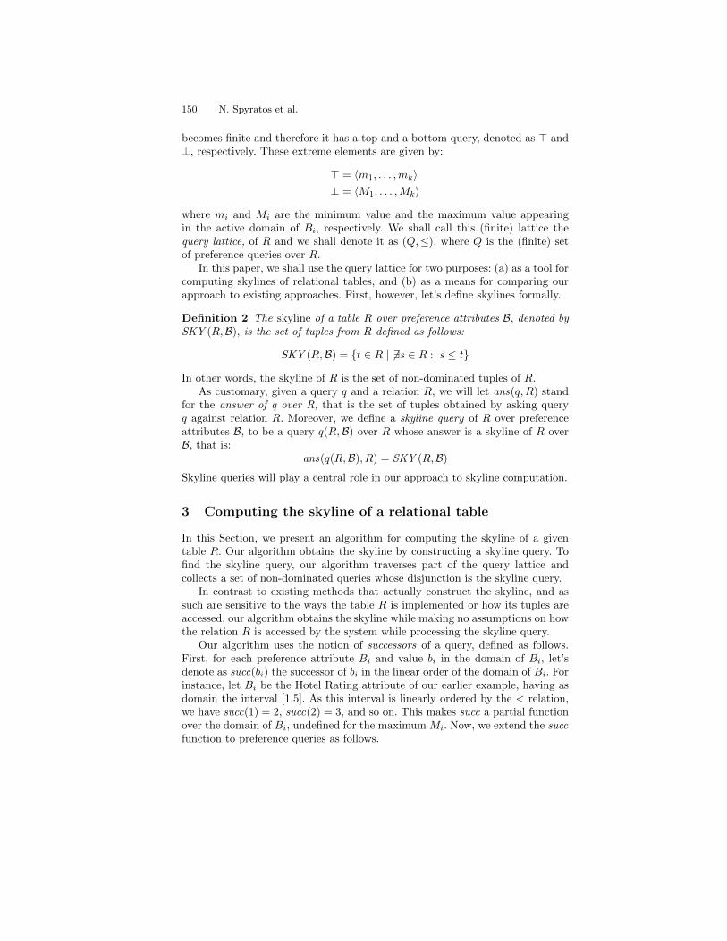
150 N. Spyratos et al.
becomes finite and therefore it has a top and a bottom query, denoted as > and⊥, respectively. These extreme elements are given by:
> = 〈m1, . . . ,mk〉⊥ = 〈M1, . . . ,Mk〉
where mi and Mi are the minimum value and the maximum value appearingin the active domain of Bi, respectively. We shall call this (finite) lattice thequery lattice, of R and we shall denote it as (Q,≤), where Q is the (finite) setof preference queries over R.
In this paper, we shall use the query lattice for two purposes: (a) as a tool forcomputing skylines of relational tables, and (b) as a means for comparing ourapproach to existing approaches. First, however, let’s define skylines formally.
Definition 2 The skyline of a table R over preference attributes B, denoted bySKY (R,B), is the set of tuples from R defined as follows:
SKY (R,B) = t ∈ R | 6 ∃s ∈ R : s ≤ t
In other words, the skyline of R is the set of non-dominated tuples of R.As customary, given a query q and a relation R, we will let ans(q,R) stand
for the answer of q over R, that is the set of tuples obtained by asking queryq against relation R. Moreover, we define a skyline query of R over preferenceattributes B, to be a query q(R,B) over R whose answer is a skyline of R overB, that is:
ans(q(R,B), R) = SKY (R,B)
Skyline queries will play a central role in our approach to skyline computation.
3 Computing the skyline of a relational table
In this Section, we present an algorithm for computing the skyline of a giventable R. Our algorithm obtains the skyline by constructing a skyline query. Tofind the skyline query, our algorithm traverses part of the query lattice andcollects a set of non-dominated queries whose disjunction is the skyline query.
In contrast to existing methods that actually construct the skyline, and assuch are sensitive to the ways the table R is implemented or how its tuples areaccessed, our algorithm obtains the skyline while making no assumptions on howthe relation R is accessed by the system while processing the skyline query.
Our algorithm uses the notion of successors of a query, defined as follows.First, for each preference attribute Bi and value bi in the domain of Bi, let’sdenote as succ(bi) the successor of bi in the linear order of the domain of Bi. Forinstance, let Bi be the Hotel Rating attribute of our earlier example, having asdomain the interval [1,5]. As this interval is linearly ordered by the < relation,we have succ(1) = 2, succ(2) = 3, and so on. This makes succ a partial functionover the domain of Bi, undefined for the maximum Mi. Now, we extend the succfunction to preference queries as follows.

Computing the Skyline of a Relational Table Based on a Query Lattice 151
Let q be a preference query q = 〈b1, . . . , bk〉 such that q 6= ⊥. This means thatbj 6= Mj for at least one j ∈ [1, k], where Mj is the maximum value in the activedomain of Bj . With no loss of generality, we shall assume that the m values of qthat are not maximal, where 1 ≤ m ≤ k, occur in the first m positions of q, (i.e.,q = 〈b1, . . . , bm,Mm+1, . . . ,Mk〉). Then, the successors of q, succ(q), is definedto be the set of queries succ(q) = q1, . . . , qm, such that, for all 1 ≤ i ≤ m,
qi = 〈b1, . . . , bi−1, succ(bi), bi+1, . . . , bm,Mm+1, . . . ,Mk〉
Clearly, the succ function is undefined on the bottom of the lattice ⊥. Thefollowing Lemma gives two important properties of the successors of q for theestablishment of the correctness of the following algorithm for computing a sky-line query of the table R.
Lemma 1. Let q be a preference query. Then, for each query q′ ∈ succ(q) :
1. q ≤ q′2. there is no query q′′ such that q < q′′ < q′.
We are now ready to give the algorithm for computing a skyline query of atable R.
Algorithm Skyline Query over a Single Table (SQST )
Input A non-empty table R, a non-empty set B = B1, . . . , Bk of preferenceattributes in R, and the projections of R over B1, . . . , Bk.
Data We use the following variables for accumulating data during the executionof the algorithm:
– The variable F is a set variable called frontier; it is initialized to empty, andit is used to accumulate the queries whose disjunction will be the result ofthe algorithm (i.e., whose disjunction will be the skyline query).
– The variable C is a set variable containing the set of all current candidatequeries; it is initialized to the top > of the query lattice.
– The variable S is a set variable used to accumulate successors of currentcandidate queries.
– The variable C ′ is a (auxiliary) set variable for accumulating candidatequeries for the next while-loop iteration in the algorithm; it is initializedto empty at the beginning of each iteration.
Output A set of preference queries over R, whose disjunction is a skyline query.
Method
C ← >;F ← ∅while C 6= ∅ do
for all c ∈ C such that ans(c,R) 6= ∅ doC ← C\c;F ← F ∪ c
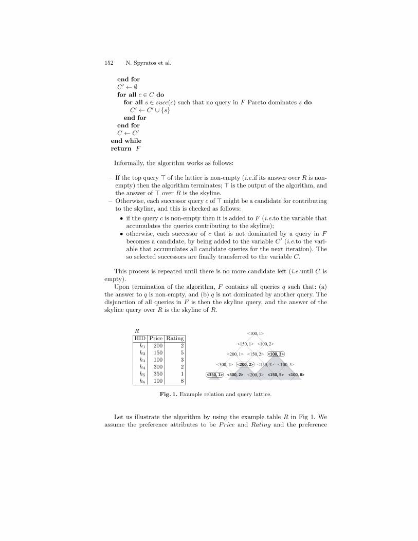
152 N. Spyratos et al.
end forC ′ ← ∅for all c ∈ C do
for all s ∈ succ(c) such that no query in F Pareto dominates s doC ′ ← C ′ ∪ s
end forend forC ← C ′
end whilereturn F
Informally, the algorithm works as follows:
– If the top query > of the lattice is non-empty (i.e.if its answer over R is non-empty) then the algorithm terminates; > is the output of the algorithm, andthe answer of > over R is the skyline.
– Otherwise, each successor query c of > might be a candidate for contributingto the skyline, and this is checked as follows:
• if the query c is non-empty then it is added to F (i.e.to the variable thataccumulates the queries contributing to the skyline);
• otherwise, each successor of c that is not dominated by a query in Fbecomes a candidate, by being added to the variable C ′ (i.e.to the vari-able that accumulates all candidate queries for the next iteration). Theso selected successors are finally transferred to the variable C.
This process is repeated until there is no more candidate left (i.e.until C isempty).
Upon termination of the algorithm, F contains all queries q such that: (a)the answer to q is non-empty, and (b) q is not dominated by another query. Thedisjunction of all queries in F is then the skyline query, and the answer of theskyline query over R is the skyline of R.
R
HID Price Rating
h1 200 2h2 150 5h3 100 3h4 300 2h5 350 1h6 100 8
Fig. 1. Example relation and query lattice.
Let us illustrate the algorithm by using the example table R in Fig 1. Weassume the preference attributes to be Price and Rating and the preference

Computing the Skyline of a Relational Table Based on a Query Lattice 153
to be Price → min and Rating → min. The projections of R over Price andRating, sorted in ascending order, are as follows:
– Price : 100, 150, 200, 300, 350– Rating : 1, 2, 3, 5, 8
The diagram in Fig 1 shows a part of the query lattice derived from R. Inthis diagram, queries having non-empty answers are emphasized by bold letters.Queries contributing to the skyline are enclosed by rounded rectangles. Graytriangles in the diagram represent areas dominated by queries in the skyline. Aswe can see in the diagram, the top of the query lattice is > = 〈100, 1〉. Therefore,we start the first iteration of the algorithm with C = 〈100, 1〉 and F = ∅. Atthe end of each subsequent iteration of the while-loop, the contents of C and Fchange as follows:
– end of 1st iteration: C = 〈150, 1〉, 〈100, 2〉, F = ∅– end of 2nd iteration: C = 〈200, 1〉, 〈150, 2〉, 〈100, 3〉, F = ∅
In the third iteration, the query 〈100, 3〉 ∈ C has a non-empty result therefore〈100, 3〉 leaves C and enters F . We then consider the successors of the queriesleft in C. 〈150, 3〉 ∈ succ(〈150, 2〉) is dominated by 〈100, 3〉 ∈ F therefore 〈150, 3〉is omitted from C ′, which accumulates candidate queries for the next iteration.
– end of 3rd iteration: C = 〈300, 1〉, 〈200, 2〉, F = 〈100, 3〉– end of 4th iteration: C = 〈350, 1〉, F = 〈100, 3〉, 〈200, 2〉– end of 5th iteration: C = ∅, F = 〈100, 3〉, 〈200, 2〉, 〈350, 1〉
(the algorithm stops here)
The correctness of the algorithm is easily established by observing that thealgorithm explores the lattice completely (this is guaranteed by the second prop-erty of the succ function in the above Lemma), retaining only maximal queries(this is guaranteed by the test on dominance performed by the algorithm andalso by the fact that the successors of a query are all dominated by it, as statedby the first property of the succ function in the above Lemma).
Formally, we will denote as SQST (R,B) the result of the SQST algorithmhaving R and B as the input non-empty relation and preference attributes, re-spectively. On the basis of the above observations, we state the following:
Proposition 1 For every relation R and preference attributes B over R,
ans(∨
SQST (R,B), R) = SKY (R,B)
We note that, as all queries in F are conjunctive and any two queries in Fdiffer in at least one conjunct, the answers making up the skyline actually forma partition of the skyline. This is an interesting observation when combined withthe notion of rank of a query in the query lattice.

154 N. Spyratos et al.
Definition 3 (Rank of a query) The rank of a query q in the query lattice isdefined as follows: if q is the root query then rank(q) = 0 else rank(q) is themaximum length of path from the root query to q
Clearly, the higher the rank of a query the less the tuples in its answer arepreferred.
Now, as the skyline of R is partitioned by the answers to the queries in F ,one can ask new kinds of queries. For example, one can ask the query: “give methe best tuples from the skyline”. The answer to this query will be the answerto the query of lowest rank in F . Similarly, one can ask the query: “give me theranks of all tuples in the skyline”. This query will return a set of ranks, therebygiving a useful information as to how far are the tuples of the skyline from themost preferred tuples. A detailed discussion of the relationship between “mostpreferred” and “non-dominated” tuples is given in a forthcoming paper.
4 Skylines of joins
We now consider the computation of the skyline over the join of two tables R1
and R2. To this end, we introduce the necessary concepts.Let R1 and R2 be relations with A1
1, . . . , An11 and A1
2, . . . , An22 as attributes,
respectively, and let Bi = B1i , . . . , B
kii , ki ≤ ni, be a set of attributes of Ri,
called the preference attributes of Ri, for i = 1, 2.We shall denote as (Q1,≤1) and (Q2,≤2) the query lattices over R1 and R2,
respectively. Moreover, ⊗i and ⊕i will stand for the least upper bound and thegreatest lower bound of any two preference queries over Ri, respectively.
Let Ji = J1i , . . . , J
li, be a set of attributes of Ri disjoint form the preference
attributes Bi, for i = 1, 2.A join over J1 and J2 is a relational equijoinR1 ./e R2,whose join expression e is given by J1
1 = J12 , . . . , J
l1 = J l
2. In order to simplifythe model and with no loss of generality, we will consider the join attributes tobe the same for the two relations, that is J1 = J2, and moreover to consist of asingle attribute J, that is e is given by J = J.
Intuitively, a preference query over a join R1 ./e R2 is a (k1+k2)-tuple whosefirst k1 elements make up a query in Q1 and whose last k2 elements make up aquery in Q2. In order to simplify notation, we will commit a slight abuse andwrite 〈q1, q2〉 to represent a preference query over R1 ./e R2, where q1 ∈ Q1 andq2 ∈ Q2. As a consequence, the set of preference queries over R1 ./e R2, that weshall denote as Q./, is given by the Cartesian product of the set of preferencequeries over R1 and R2, that is:
Q./ = Q1 ×Q2
Now, let ≤./ be the Pareto preference relation over Q./. As we have alreadyseen in the previous Section, (Q./,≤./) is a complete lattice. Moreover, it is notdifficult to see that:

Computing the Skyline of a Relational Table Based on a Query Lattice 155
Proposition 2 (Q./,≤./) is the product of (Q1,≤1) and (Q2,≤2). That is, let-ting q and q′ be preference queries in Q./ such that q = 〈q1, q2〉 and q′ = 〈q′1, q′2〉,where q1, q
′1 ∈ Q1 and q2, q
′2 ∈ Q2, we have:
1. q≤./q′ iff q1 ≤1 q
′1 and q2 ≤2 q
′2
2. q ⊗./ q′ = 〈q1 ⊗1 q
′1, q2 ⊗2 q
′2〉
3. q ⊕./ q′ = 〈q1 ⊕1 q
′1, q2 ⊕2 q
′2〉
From now on we shall simplify notation by omitting subscripts, unless thiscreates ambiguity.
We shall call join values the set of tuples V = X1 ∩X2, where:
Xi = πJ(Ri) for i = 1, 2
By definition of join, a tuple t in Ri contributes to the join if and only if itsprojection over the join attribute J is in V, that is t.J ∈ V, for i = 1, 2. Likewise,a query q in Qi may contribute to the skyline of the join only if it occurs in thejoin. For each join value v ∈ V, we define the v−partition of Ri, denoted Si(v),as follows :
Si(v) = πBi(σJ=v(Ri)) for i = 1, 2
In practice, each v−partition includes the queries that contribute to the joinR1 ./ R2. In particular:
πB1∪B2(R1 ./ R2) =
⋃
v∈VS1(v)× S2(v)
v−partitions play an important role in determining the skyline of the join R1 ./R2 without computing the join.
Proposition 3 A query 〈q1, q2〉 ∈ πB1∪B2(SKY (R1 ./ R2,B1∪B2)) iff for some
join value v ∈ V, qi ∈ πBi(SKY (Si(v),Bi)) for i = 1, 2 and for no other v′ ∈ V
there exists skylines q′i ∈ πBi(SKY (Si(v
′),Bi)) such that q′i ≤ qi for i = 1, 2.Proof: (→) If for some join value v ∈ V, qi ∈ πBi(SKY (Si(v),Bi)) for i = 1, 2then 〈q1, q2〉 ∈ πB1∪B2(R1 ./ R2), and moreover for 1 in Proposition 2 thereexists no other query 〈q′1, q′2〉 ∈ πB1∪B2
(R1 ./ R2) where q′i ∈ Si(v) for i =1, 2 such that 〈q′1, q′2〉 ≤ 〈q1, q2〉. If for no other v′ ∈ V there exists skylinesq′i ∈ πBi
(SKY (Si(v′),Bi)) such that q′i ≤ qi for i = 1, 2 then again from 1
in Proposition 2 there exists no 〈q′1, q′2〉 such that 〈q′1, q′2〉 ≤ 〈q1, q2〉. Hence〈q1, q2〉 ∈ πB1∪B2(SKY (R1 ./ R2,B1 ∪ B2)).(←) Suppose not. Then, either (a) for no join value v ∈ V, qi ∈ πBi(SKY (Si(v),Bi))for i = 1, 2 or (b) there exists a join value v′ ∈ V and skylines q′i ∈ πBi
(SKY (Si(v′),Bi))
such that q′i ≤ qi for i = 1, 2. In case (a), there are two sub-cases: (a1) for no joinvalue v ∈ V, qi ∈ Si(v) for i = 1, 2. In this case, 〈q1, q2〉 6∈ πB1∪B2
(R1 ./ R2),against the hypothesis. (a2) for some join value v ∈ V, qi ∈ Si(v), but eitherq1 6∈ πB1(SKY (S1(v),B1)) or q2 6∈ πB2(SKY (S2(v),B2)). Then let q′i be suchthat q′i ∈ πBi
(SKY (Si(v),Bi)). Such q′i are guaranteed to exist because Si(v) isfinite and partially ordered by Pareto preference. By hypothesis, either q′1 6= q1 or

156 N. Spyratos et al.
q′2 6= q2. Then 〈q′1, q′2〉 ∈ πB1∪B2(R1 ./ R2) and by 1 in Proposition 2 〈q′1, q′2〉 ≤〈q1, q2〉, therefore 〈q1, q2〉 6∈ πB1∪B2
(SKY (R1 ./ R2,B1∪B2)), against the hypoth-esis. (b) If there exists a join value v′ ∈ V and skylines q′i ∈ πBi
(SKY (Si(v′),Bi))
such that q′i ≤ qi for i = 1, 2 then 〈q′1, q′2〉 ∈ πB1∪B2(R1 ./ R2) and by 1 in Propo-
sition 2 〈q′1, q′2〉 ≤ 〈q1, q2〉, therefore 〈q1, q2〉 6∈ πB1∪B2(SKY (R1 ./ R2,B1 ∪ B2)),
against the hypothesis.
We now provide an algorithm for computing the skyline queries over the joinof two tables R1 and R2 (without computing the join.). The algorithm exploitsProposition 3, and uses the SQST algorithm for computing skylines over v-partitions of the given tables. As a result, the algorithm returns two sets ofqueries, one over R1, the other over R2, for selecting from each table the tuplesthat will generate the skyline of the join R1 ./ R2, and only those.
Algorithm The Skyline Queries over a Join (SQJ )
Input Non-empty relations R1 and R2, non-empty sets B1 and B2 of preferenceattributes in R1 and R2, respectively, and the join values V.
Data G is a set variable initialized to empty and used to accumulate all candidateskyline queries, resulting from the Cartesian products of the skyline queries overthe same join value. R is a set variable where the skyline of G is computed. Pi
and Fi (for i = 1, 2) are auxiliary set variables, used to store v-partitions andfinal results, respectively.
Output Two sets of queries, one over R1 and the other over R2.
Method
G← ∅for all v ∈ V doP1 ← SQST (S1(v),B1)P2 ← SQST (S2(v),B2)G← G ∪ (P1 × P2 × v)
end forR← SQST (G,B1 ∪ B2)F1 ← πB1∪J(R)F2 ← πB2∪J(R)return F1, F2
We note that the algorithm operates in three passes:
1. In the first pass, it gathers (in G) all candidate results by looping over alljoin values. This is in fact required by the first condition of Proposition 3,which states that 〈q1, q2〉 is in a skyline query of the join if both q1 and q2are skyline queries over the v-partitions for the same join value v.
2. In the second pass, it removes from G the compound queries that are dom-inated by some other compound query, as required by the second conditionof Proposition 3.

Computing the Skyline of a Relational Table Based on a Query Lattice 157
3. Finally, it slices the compound queries vertically, in order to obtain queriesover R1 (these are stored in F1) and queries over R2 (in F2). Notice thatthe join attribute J must be transferred all along in order to generate thecorrect queries.
Clearly, there is no other way of proceeding since it is necessary to obtain allcandidate queries in order to apply the second condition of Proposition 3.
Formally, we will denote as SQJ (R1, R2,B1,B2)i the i−th result of the SQJalgorithm having R1 and R2 as the input non-empty relations and B1 andB2 as preference attributes, respectively. For readability, we will abbreviateSQJ (R1, R2,B1,B2)i as SQJ i.
On the basis of the above observations and of Proposition 3, we thereforestate the following:
Proposition 4 For every pair of relations R1 and R2 and preference attributesB1 and B2 over them,
SQST (ans(∨
SQJ 1, R1) ./ ans(∨
SQJ 2, R2),B1∪B2) = SKY (R1 ./ R2,B1∪B2)
Let us demonstrate the SQJ algorithm by using table R1 (hotels) and R2
(restaurants) in Fig. 2. Suppose we want to find best combinations of hotelsand restaurants in the same “Location”, by minimizing “Price”, “Rating”, “Dis-tance” and “Location” (we took this example from [23]). In this case, the pref-erence attributes are B1 = Price,Rating, B2 = Distance,Ranking and thejoin attribute is J = Location. From the intersection of values appearing inthe Location attribute in R1 and R2, we can obtain join values V = A,B,C.
In the algorithm, firstly we gather candidate skyline queries for each joinvalue. In the example, for a join value A ∈ V , we obtain v-partition S1(A) andS2(A). Then we compute skylines P1, P2 (emphasized in tables S1, S2 by boldletters) from S1(A), S2(A) by the applying the SQST algorithm. Finally wemake a Cartesian product P1 × P2 × A and append it to G that accumulatescandidate skyline queries.
After iterating this candidate gathering process for every join value, we applySQST to G to obtain the skyline (emphasized in tables G by bold letters) overthe join R1 ./ R2. It is important to note the difference of size between R1 ./ R2
and G. In this example, R1 ./ R2 produces 12 tuples but G contains 8 tuples.Therefore, we can compute the skyline from G with less cost than by computingdirectly from R1 ./ R2.
In the example, 〈h5, r5〉 is not a skyline in the join because for the join valueB, we have h2 dominating h5 and r1 dominating r5. On the other hand, neitherh6 nor r4 are skyline in their table, but they form a skyline in the join becausethey are skylines in their join group and there is no other group in which bothare dominated (h6 is dominated by a query h3 in the A group, whereas r4 isdominated by r2 in the C group, and there is no single group in which both aredominated.)
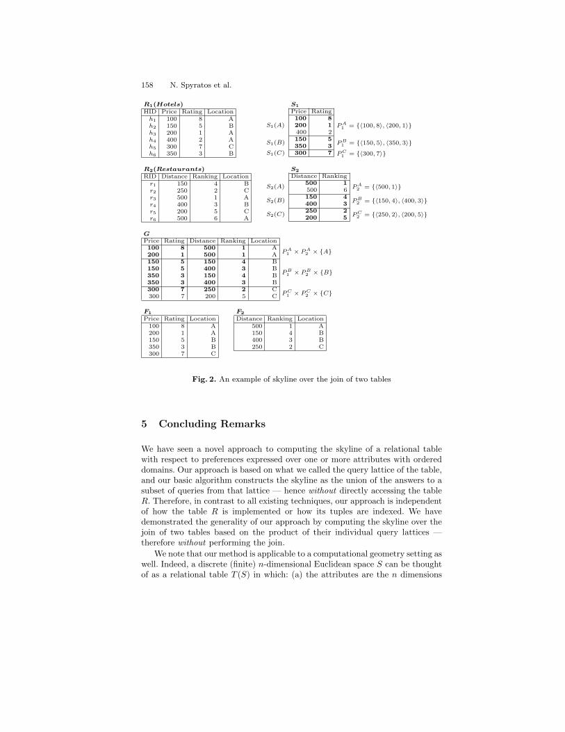
158 N. Spyratos et al.
R1(Hotels)HID Price Rating Locationh1 100 8 Ah2 150 5 Bh3 200 1 Ah4 400 2 Ah5 300 7 Ch6 350 3 B
S1
Price Rating
S1(A)100 8
PA1 = 〈100, 8〉, 〈200, 1〉200 1
400 2
S1(B)150 5
PB1 = 〈150, 5〉, 〈350, 3〉
350 3S1(C) 300 7 PC
1 = 〈300, 7〉
R2(Restaurants)RID Distance Ranking Location
r1 150 4 Br2 250 2 Cr3 500 1 Ar4 400 3 Br5 200 5 Cr6 500 6 A
S2
Distance Ranking
S2(A)500 1
PA2 = 〈500, 1〉
500 6
S2(B)150 4
PB2 = 〈150, 4〉, 〈400, 3〉
400 3
S2(C)250 2
PC2 = 〈250, 2〉, 〈200, 5〉
200 5
GPrice Rating Distance Ranking Location100 8 500 1 A
PA1 × PA
2 × A200 1 500 1 A150 5 150 4 B
PB1 × PB
2 × B150 5 400 3 B350 3 150 4 B350 3 400 3 B300 7 250 2 C
PC1 × PC
2 × C300 7 200 5 C
F1
Price Rating Location100 8 A200 1 A150 5 B350 3 B300 7 C
F2
Distance Ranking Location500 1 A150 4 B400 3 B250 2 C
Fig. 2. An example of skyline over the join of two tables
5 Concluding Remarks
We have seen a novel approach to computing the skyline of a relational tablewith respect to preferences expressed over one or more attributes with ordereddomains. Our approach is based on what we called the query lattice of the table,and our basic algorithm constructs the skyline as the union of the answers to asubset of queries from that lattice — hence without directly accessing the tableR. Therefore, in contrast to all existing techniques, our approach is independentof how the table R is implemented or how its tuples are indexed. We havedemonstrated the generality of our approach by computing the skyline over thejoin of two tables based on the product of their individual query lattices —therefore without performing the join.
We note that our method is applicable to a computational geometry setting aswell. Indeed, a discrete (finite) n-dimensional Euclidean space S can be thoughtof as a relational table T (S) in which: (a) the attributes are the n dimensions

Computing the Skyline of a Relational Table Based on a Query Lattice 159
of S and (b) each tuple of T (S) represents a point in S. Moreover, the answerto a query q = 〈b1, . . . , bk〉 from the query lattice of T (S) is the set of allpoints of S such that (B1 = b1) ∧ . . . ∧ (Bk = bk), where B1, . . . , Bk are thecorresponding dimensions; in other words, the answer to q is the set of pointshaving the same coordinate values over the dimensions B1, . . . , Bk. Additionally,our method can be applied to the Cartesian product of two or more spacesthrough the product lattice of the individual spaces. We are currently pursuingwork in two different directions, namely refining skyline analysis and applyingour approach to a distributed setting:
1. Refining skyline analysisAs we mentioned in section 3, the skyline query returned by our basic al-gorithm is the disjunction of a set of queries from the query lattice, sayq1 ∧ . . .∧ qm; and the answers to these queries actually partition the skylineinto disjoint subsets. Moreover, these queries have different ranks, in general.Therefore it now becomes possible to ask finer queries regarding the skylinesuch as “give me the best tuples of the skyline” (meaning the answer to thequery qi of highest rank), or “return the skyline by presenting the answersto qi’s in increasing order of rank”, and so on. In this respect, we would alsolike to investigate in more detail the relationship between “most preferredtuple” and “non-dominated tuple”.
2. Applying our method to a distributed settingAs information systems store bigger and bigger volumes of data today, datamanagement and in particular query processing presents difficult challenges.From the user viewpoint, big volumes of data imply answers of large size.By returning the best tuples (in terms of user preferences), the skyline queryrelieves the user from having to deal with answers of large size; and havingthe possibility to further refine the skyline (as mentioned above) furthercontributes in that direction. However, in recent years, data management anddata storage have become increasingly distributed, and distribution presentsadditional challenges for query processing. Adapting the skyline operator to adistributed setting is one of the research lines that we are currently pursuing.We believe that our approach to skyline computation through query latticesis particularly well suited in a distributed environment, where computationcan be distributed and recomposed in the form of the product lattice.
References
1. I. Bartolini, P. Ciaccia, and M. Patella. SaLSa: computing the skyline withoutscanning the whole sky. In Proceedings of CIKM, 2006.
2. I. Bartolini, P. Ciaccia, and M. Patella. Efficient sort-based skyline evaluation.ACM Trans. Database Syst., 33(4), 2008.
3. S. Borzsonyi, D. Kossmann, and K. Stocker. The skyline operator. In Proceed-ings of ICDE, pages 421-430, 2001.
4. C.-Y. Chan, P.-K. Eng, K.-L. Tan. Stratified computation of skylines withpartially-ordered domains. In Proc. of SIGMOD 2005, pp. 03–214, 2008.

160 N. Spyratos et al.
5. J. Chomicki, P. Godfrey, J. Gryz, and D. Liang. Skyline with presorting. InProceedings of ICDE, pages 717-816, 2003.
6. B. Cui, H. Lu, Q. Xu, L. Chen, Y. Dai, Y. Zhou. Parallel Distributed Processingof Constrained Skyline Queries by Filtering. In Proc. of ICDE 2008, pp. 546-555, 2008.
7. P. Godfrey, R. Shipley, and Jarek Gryz. Algorithms and analyses for maximalvector computation. The VLDB Journal, vol 16(1), pp. 5–28, 2007.
8. W. Jin, M. Ester, Z. Hu, and J. Han. The multi-relational skyline operator. InProceedings of ICDE, 2007.
9. W. Jin, M. Morse, J. Patel, M. Ester, and Z. Hu. Evaluating skylines in thepresence of equi-joins. In Proc. of ICDE, 2010.
10. N. Koudas, C. Li, A. K. H. Tung, and R. Vernica. Relaxing join and selectionqueries. In Proceedings of VLDB, 2006.
11. H.T. Kung, F. Luccio, F.P. Preparata. On finding the maxima of a set ofvectors. Journal of the ACM, vol. 22(4), pp. 469–476, 1975.
12. M.E. Khalefa, M.F. Mokbel, J.J. Levandoski. Skyline Query Processing forIncomplete Data. In Proc. of ICDE 2008, pp. 556-565, 2008.
13. D. Kossmann , F. Ramsak , S. Rost. Shooting Stars in the Sky: An OnlineAlgorithm for Skyline Queries. In Proc. of VLDB 2002, pp. 275–286, 2002.
14. X. Lin , Y. Yuan , W. Wangnicta , S. Wales. Stabbing the sky: Efficient skylinecomputation over sliding windows. In Proc. of ICDE 2005, pp. 502–513, 2005.
15. M. Morse , J. Patel , H. V. Jagadish. Efficient Skyline Computation over Low-Cardinality Domains. In Proc. of VLDB 2007, pp. 267–278, 2007.
16. J. Pei , W. Jin , M. Ester , Y. Tao. Catching the best views of skyline: Asemantic approach based on decisive subspaces. In Proc. of VLDB 2005, pp.253–264, 2005.
17. J. Pei , B. Jiang , X. Lin , Y. Yuan. Probabilistic skylines on uncertain data.In Proc. of VLDB 2007, pp. 15–26, 2007.
18. F.P. Preparata, M.I. Shamos. Computational Geometry Computational Geom-etry, Springer-Verlag, 1985.
19. D. Papadias, Yufei Tao, Greg Fu, Bernhard Seeger. An Optimal and ProgressiveAlgorithm for Skyline Queries. In Proc. of SIGMOD 2003, pp. 467–478, 2003.
20. V. Raghavan, E. Rundensteiner. Progressive result generation for multi-criteriadecision support queries. In Proceedings of ICDE, 2010.
21. K.-L. Tan, P.-K. Eng, B.C. Ooi. Efficient Progressive Skyline Computation. InProc. of VLDB 2001, pp. 301-310, 2001.
22. Y. Tao, X. Xiao, and J. Pei. Subsky: Efficient computation of skylines in sub-spaces. In Proceedings of ICDE, 2006.
23. A. Vlachou, C. Doulkeridis, N. Polyzotis. Skyline query processing over joins.In Proceedings of SIGMOD 2011, pp. 73–84, 2011.
24. A. Vlachou, K. Nørvag. Bandwidth-constrained distributed skyline computa-tion. In Proc. of MobiDE 2009, pp. 17–24, 2009.
25. D. Sun, S. Wu, J. Li, and A. K. H. Tung. Skyline-join in distributed databases.In ICDE Workshops, 2008.
26. Q. Wan, R. C.-W. Wong, I. F. Ilyas, M. T. Ozsu, and Y. Peng. Creatingcompetitive products. PVLDB, vol. 2(1), 898-909, 2009.
27. P. Wu , C. Zhang , Y. Feng , B.Y. Zhao , D. Agrawal , A.E. Abbadi. Parallelizingskyline queries for scalable distribution. In Proc. of EDBT 2006, pp. 112-130,2006.
28. Y. Yuan , X. Lin , Q. Liu , W. Wang , J.X. Yu , Q. Zhang. Efficient Computationof the Skyline Cube. In Proc. of VLDB 2005, pp. 241–252, 2005.

Computing the Skyline of a Relational Table Based on a Query Lattice 161
29. S. Zhang , N. Mamoulis , S.W. Cheung. Scalable skyline computation usingobject-based space partitioning. In Proc. of SIGMOD 2009, pp. 483-494, 2009.

Using FCA for Modelling Conceptual Difficulties inLearning Processes
Uta Priss, Peter Riegler, Nils Jensen
Zentrum fur erfolgreiches Lehren und LernenOstfalia University of Applied Sciences
Wolfenbuttel, Germanywww.upriss.org.uk, p.riegler,[email protected]
Abstract. In the natural sciences, mathematics and technical subjects, universi-ties often observe generally low pass rates and high drop out rates in the firstyears. Many students seem to have conceptual difficulties with technical andmathematical materials. Furthermore, physics education research appears to indi-cate that even students who are able to pass exams may still not have a good un-derstanding of basic physics concepts. Some researchers use the notion of “mis-conception” to describe conceptual differences between intuitive notions and ac-cepted scientific notions. A significant body of educational research exists dedi-cated to overcoming such didactic challenges, but so far not much Formal Con-cept Analysis (FCA) research has been dedicated to these topics. The aim of thispaper is to develop a better understanding of the structure of conceptual difficul-ties in learning processes using FCA. It is not intended in this paper to developnew educational methods or to collect new data, but instead to analyse existingdata and models from an FCA viewpoint.
1 Introduction
Education is an interesting application area for Formal Concept Analysis1 (FCA) be-cause the analysis, representation and development of conceptual structures - in themind of the learner, and maybe also of the teacher - is an inherent feature of learningand teaching. Because modern e-learning materials and environments tend to accumu-late and provide large amounts of data, any technology, such as FCA, developed forstructuring and retrieval of information or semantic, conceptual and ontological analy-sis is implicitly applicable to learning materials as well.
Rudolf Wille the founder of FCA also pioneered the use of FCA for teaching math-ematics (Wille, 1995). He published a number of subsequent papers on mathematicsrestructuring and education - most of them are more general, of philosophical natureand not specifically about FCA. Otherwise, there do not appear to be significant num-bers of FCA publications in the educational domain. Examples of FCA applications inthis area focus on ontological representations, such as the structuring, retrieval and vi-sualisation of learning materials (Lee, 2005) or the development of an ontology-based
1 Because this conference is dedicated to FCA, this paper does not provide an introduction toFCA. Information about FCA can be found, for example, on-line (http://www.fcahome.org.uk)and in the main FCA textbook by Ganter & Wille (1999).

162 U. Priss et al.
courseware management system (Tane et al., 2004) which facilitates browsing, query-ing and clustering of materials and ontology evolution. Other FCA applications relateto the use of FCA with computer algebra systems (Priss, 2010) and to the meta-analysisof learning materials. For example Pecheanu et al. (2011) use FCA to evaluate andcompare open source learning platforms.
Apart from the general data analysis and knowledge representation applications, itis of interest to use FCA to directly analyse the cognitive structures involved in learn-ing processes because presumably learning consists of concept formation, ordering andstructuring. Applying FCA in this area is not fundamentally different from other appli-cations where different concept lattices might represent the views of different expertsexcept that in teaching there is an expectation that some conceptual structures are cor-rect and some are not and that the conceptual structures of the students are intended tochange.
One obvious difficulty is that it is not easy to obtain representations of such cogni-tive structures. Psychologists have developed methods for eliciting and externally rep-resenting mental models. A number of applications of FCA in the psychological do-main have been described, for example, by Spangenberg and Wolff (1991). Al-Dibanand Ifenthaler (2011) discuss the comparison of two methods for eliciting and analysingmental models of students, one of which uses FCA. These methods build on a qualitativeanalysis of data, including transcribed and coded textual protocols, and data collectedfrom specific tests where subjects order concepts in if-then relations. A disadvantageof these methods is that it is not clear whether they could be applied to data observedin real teaching situations (instead of collected from tests) because real data might nothave sufficient structure and detail. Furthermore at least in the Al-Diban and Ifenthalerstudy, the focus was on declarative knowledge, that is whether students know certainfacts, not so much on degrees of understanding. An advantage of these methods is that,for example, conceptual gaps and differences among different students and betweenstudents and teachers can be detected and analysed.
In addition to the analysis of conceptual structures in learning processes, one mightalso want to model the conceptual space of a domain for teaching purposes. This hasbeen achieved by Falmagne et al. (2006) who describe a “knowledge state” as the set ofparticular problems a student can answer in a mathematical topic area. Feasible knowl-edge states are represented with respect to a precedence graph. This graph is a partiallyordered set and not a lattice, but it could be embedded into a lattice and thus modelledwith FCA. The idea is that knowledge is ordered: if someone masters a certain mathe-matical problem then that person can also solve problems that are simpler but may stillhave to learn to solve problems that are more difficult. Because the precedence graph isnot a linear order, different students can take different learning paths. The position ofthe knowledge state of a student in the graph shows exactly which problems the studentcan attempt to learn to solve next. Furthermore the student’s progress can be exactlymeasured. Establishing a precedence graph for a mathematical topic area which mightconsist of hundreds of states is labour-intensive but feasible in a commercial environ-ment such as Falmagne et al.’s ALEKS software tool. There are different means forbuilding such a precedence graph: by questioning experts about the difficulties and pre-

Using FCA for Modelling Conceptual Difficulties in Learning Processes 163
requisites of problems, by analysing student data collected from an e-learning tool orby analysing problem solving processes in the domain.
Currently, ALEKS focuses on mathematics and science topics. It is not clear howfar such approaches would be suitable for other non-science domains where it would bedifficult to establish a precise ordering of problems. Furthermore, it it may be difficult toevaluate how accurate and useful a particular precedence graph is because user testingof complex e-learning tools is notoriously difficult. If student learning improves whilethey are using ALEKS, it would be difficult to determine whether that is because of theprecedence graph or because of any other of ALEKS’s many features.
In summary, general knowledge representation and retrieval aspects of e-learningtools are not any different to such aspects of other textual databases and are coveredsufficiently in other domains than educational research. But the analysis of concep-tual structures involved in learning processes and the conceptual structuring of domainknowledge for learning purposes is specific to educational research. Currently, FCAappears to be underrepresented in these tasks but it should be very applicable to bothof these tasks. It is of particular interest to study differences between the conceptualstructures of a learner and of an expert, such as knowledge gaps, discrepancies and mis-conceptions. A goal for this paper is to involve FCA in the analysis, description anddetection of conceptual difficulties, including misconceptions. Section 2 of this paperprovides an overview of challenges encountered in teaching conceptually difficult top-ics. The following three sections show examples of conceptual difficulties for selectedmathematical topics: equality in Section 3, translating text into algebraic expressionsin Section 4 and the notion of “function” in Section 5. The lattices in these examplesare developed from the viewpoint of a teacher who is exploring the difficulties in theseareas by modelling formal contexts based on the description of misconceptions in theliterature and based on student data.
2 Successful and unsuccessful teaching
Physics Education Research studies the problems students have in acquiring physicsconcepts. Hake (1998) explains that students have initial common-sense beliefs about’motion’ which are in contradiction to current physics theory and which are not im-proved on by traditional educational methods. Hestenes et al. (1992) published a ForceConcept Inventory (FCI) designed to test the students’ conceptual understanding ofNewtonian mechanics which can be used before and after a physics course to evaluatethe educational success of the course. The test is written in a language that is accessi-ble to people who have never taken physics courses but the test is quite different fromstandard exams which students may be able to pass by memorising and applying for-mulas. The FCI test purely examines conceptual knowledge. It shows that there is nocorrelation between standard exam results and test results of individual students. Manystudents do not change their incorrect beliefs about physics concepts when they aretaking physics classes. The revelation that traditional teaching methods are largely in-effective (Hake, 1998) led physics professors to search for alternative teaching methodsand led to the establishment of Physics Education Research as a field of study. It seemsthat misconceptions are particularly visible in physics education because, on the one

164 U. Priss et al.
hand, people have naive physics theories about natural laws based on observation andexperience and, on the other hand, scientific physics theory describes concepts and lawswith mathematical precision which are experimentally verifiable but which sometimescontradict naive observation and experience. Outside the natural sciences, concepts arenot usually definable and verifiable with such rigour and precision. But the insights ofPhysics Education Research should also be relevant for the other natural sciences andmathematics (the latter as discussed by Riegler (2010)).
A conclusion of Physics Education Research is that teaching methods involvinginteractive engagement (Hake, 1998) tend to be more successful in improving the con-ceptual understanding of students than traditional teaching methods. Interactive engage-ment is achieved by questioning and challenging students to think instead of just mem-orising facts. Several factors appear to be contributing to the success of interactive en-gagement teaching, including cognitive, social constructive and psychological factors.
From a cognitive viewpoint, it has been known for many years (Auble and Franks,1978) that effort toward comprehension improves recall, i.e., if someone makes an ef-fort at finding a solution before the solution is presented, recall is higher than if a solu-tion is presented right away. Furthermore, active recall is more beneficial for long-termretention than passive exposure (Ellis, 1995). Conway et al. (1992) report that course-work marks are a better predictor for long-term retention than exam marks, possiblybecause creating a piece of coursework requires the students to be involved with thesubject matter at a deeper level than when they reiterate facts during an exam. Conwayet al.’s (1992) paper also confirms other observations of Physics Education Researchwith respect to other domains: procedural knowledge (where students learn somethingby doing it) is retained much better than declarative knowledge. Students who take onlyone course in a subject domain tend to forget it completely after a few years. In par-ticular although they might remember some isolated facts, their understanding of thesubject is first to disappear - presumably because they never really understood it in thefirst place. Students who take several courses on a topic and achieve a certain level ofproficiency and understanding will retain a large portion of their knowledge for a longtime. Thus if interactive engagement teaching leads to a better understanding of a sub-ject, it will help students to remember what they have learnt more permanently than justuntil the end of the term.
An example of interactive engagement teaching is Mazur’s (1996) peer instructionwhich is even feasible in large classes. Using peer instruction, a lecturer pauses a lecturewith challenging questions which the students discuss among each other. Apparentlystudents do not change their conceptual knowledge just because a teacher provides themwith facts or a good explanation or even with a demonstration. But if they discussquestions among each other, the students who do have correct conceptual understandingtend to be able to convince their peers. In addition to the cognitive aspects of interactiveengagement learning, there seems to be a social component involved: peer pressureseems to be a stronger motivation for people to question and change their beliefs thanexplanation or observation.
Last but not least, psychological aspects are involved in learning processes. Devlin(2000) argues that mathematicians are psychologically different to non-mathematiciansbecause mathematicians think about mathematical objects in an emotional, associa-

Using FCA for Modelling Conceptual Difficulties in Learning Processes 165
tive manner in the same way as other people think about physical or even animate ob-jects. For example, mathematicians might attribute emotional features to numbers andother abstract objects. Other psychological aspects are involved when people experi-ence clashes between observation and scientific explanations, as for example in opticalillusions which are clashes of visual perception and logical, geometrical explanations.Some people perceive clashes as emotionally upsetting. A famous example is the MontyHall problem2 about the winning chances in a game show. When Marilyn Vos Savantdiscussed it and similar problems in her column in the TV magazine Parade, readersresponded with angry, emotional letters: “I will never read your column again3” or “Asa professional mathematician, I’m very concerned with the general public’s lack ofmathematical skills. Please help by confessing your error and in the future being morecareful4.” - written by someone with a Ph.D who was wrong! One can speculate thatanimals have evolved probabilistic intuitions in order to make survival decisions whichevoke strong emotional responses when challenged. Another example of intuitions con-tradicting mathematical probability is the belief which many people have that the longerthey have played in the lottery without winning, the more likely it is that they are goingto win the next time they play. Again this belief tends to have an emotional componentas anybody can observe who has ever discussed it with lottery players.
In summary, teaching a topic which contradicts the existing conceptual structureswhich the students have is challenging. Methods such as peer instruction can help toovercome cognitive, social constructivist and emotional obstacles. Clearly, not all top-ics evoke such difficulties and some can be taught with more standard teaching meth-ods. Thus it would be useful for a teacher to know in advance which areas of the sub-ject domain are going to produce conceptual difficulties and which not. McDermott(2001) argues that there is only a limited number of re-occurring conceptual difficul-ties which tend to be experienced by all students similarly. The idea for this paper isthat FCA might provide useful methods for detecting and analysing conceptual diffi-culties. Although McDermott (2001) emphasises that just detecting misconceptions isnot sufficient for improving teaching, providing a better understanding of the concep-tual structures of misconceptions is going to be beneficial for teachers. In the following,three examples of conceptual difficulties in mathematics education are analysed usingFCA.
3 Conceptual difficulties of the equality sign
Prediger (2010) discusses problems pupils are having with developing an appropriateconceptual model of equality. In primary school, pupils tend to experience the equalsign as a request to calculate something. For example, “2 + 3 =” might be printed in atextbook. Prediger calls this the operational use because pupils are requested to performan operation. Apparently, this can lead to difficulties later when the equal sign is used inits more general algebraic meaning (or its “relational” meaning). For example, Predigerquotes the case of a pupil who says that the equation 24 × 7 = 20 × 7 + 4 × 7 is
2 http://en.wikipedia.org/wiki/Monty Hall problem3 Parade Magazine, July 27, 19974 http://www.marilynvossavant.com/articles/gameshow.html

166 U. Priss et al.
wrong because “24×7 does not equal 20” and the case of a pupil who writes “1×10 =10 + 110 = 120”. Prediger then discusses the difficulties which prospective teachersmight encounter in understanding the problems these pupils are having. In her analysisshe distinguishes operational, relational and specification uses (such as defining x :=4) of the equal sign. She divides the relational use further into symmetric identities(4 + 5 = 5 + 4), general equivalences ((a − b)(a + b) = a2 − b2), searching forunknowns (x2 = 6 − x) and contextual uses (a2 + b2 = c2) where the variables aremeaningful in a context, such as characterising a right-angled triangle.
To demonstrate the use of FCA in this area we have modelled the problem as aformal context. The formal objects are examples of uses of the equal sign, inequality(>) and equivalence (⇔). Furthermore we added basic operations from programminglanguages: not-equal (!=), test for equality (==) and Boolean operators (&&). Fourof the formal attributes are from Prediger’s classification: “operation”, “contextual”,“definition” (i.e. specification) and “law” (i.e equivalence). Here, “operation” refers torule-based drills where the students solve a problem in a precisely taught manner andthe equality sign is always read from left to right. A “definition” for other symbolsthan “=” defines a set of possible values for a variable (e.g., i > 1). Furthermore, twoattributes have been added which distinguish whether the statements are true for allvalues of the variables or just for some. Prediger’s “unknowns” has been replaced with“test” as a request to evaluate an expression with respect to variables with given values.
contextual
<=>
x − y = (x−y)(x+y)22a + b = c2 2 2
x := 42+3 =
2+y = 6x != 4
i > 1
test
x=4 y=5&&x == 4
x>4 −x<−4
for some values
law
3 != 4y+1 > y
x+y = y+x
for all values definition operation
y:=4 x==3:<=>
Fig. 1. Equation, assignment and comparison operators

Using FCA for Modelling Conceptual Difficulties in Learning Processes 167
The resulting concept lattice (Fig. 1) shows a classification which is slightly differ-ent from Prediger’s list5. The operational use of the equal sign is not connected to any ofthe other uses. Although this results directly from the definition of the formal attribute“operation”, it represents implicit structure which the authors were not aware of be-fore the lattice was constructed. The separation of “operation” from the other conceptsprovides a graphical explanation as to why students may find it particularly difficult toprogress from an operational use to the more general algebraic use.
The extensions of the concepts under “for all values” contain tautologies. But thereis a distinction made between those which students have to specifically learn (under“law”) in order to understand how the operators work and those which just happento be true. There are three different reasons why a statement might only be true forsome values of the variables: the variables are defined in the statement; it is to be testedwhether the statement is true (or for which variables it is true); and in the contextualuse, the statement is only true in some contexts and thus describes such contexts. Someinteresting cases are under both “test” and “definition”: an equation 2 + y = 6 is bothan implicit definition of y and a request to evaluate which values of y yield the equationto be true. For the use of != and <, it depends on the context whether the statements aremeant to be evaluated for their truth value or whether they are meant to define a rangefor their variables.
4 Conceptual difficulties of translating text into algebraicexpressions
A well-known conceptual difficulty that mathematics students experience pertains to thetranslation of text into algebraic expressions. Clement (1982) conducts an experimentwhere he asks students to write an equation using the variables S and P to represent“there are six times as many students as professors”. His findings are that only 40-60% of the students produce a correct answer (S = 6P ). The most common incorrectanswer is 6S = P . He provides two reasons for the incorrect answer: first, some stu-dents simply translate the sentence into mathematical symbols in the same word order.Second, some students use a static comparison pattern or, in other words, an incorrectschema where S and P do not represent numbers, but instead units of students andprofessors. This is in the same manner as how m and km are used in 1000m = 1km.In this case, m and km are not variables but represent a fixed “1 to 1000” relation-ship. It is not possible to substitute arbitrary values for m or km, but m can be sub-stituted with 1
1000km and km can be substituted with 1000m, yielding, for example,2000m = 2000 × 1
1000km = 2km. One difference between units and variables fornumbers is that it is not usually acceptable to insert a multiplication sign between anumber and its unit.
Table 1 summarises the differences between the two conceptual systems: in the firstone the letters represent units, in the second, algebraic one the letters represent vari-ables for numbers. The first conceptual system has a meronymic (part-whole) quality.A certain, fixed aggregate of the smaller units constitutes the larger unit. The extension
5 In Fig. 1, in the statements with more than one operator the relevant one is printed in bold face.
168 U. Priss et al.
of 6s = 1p is really a fixed “6 to 1” relation which is expressed in s and p. In contrast,the algebraic conceptual system represents normal algebraic use of variables. The ex-tension of s = 6 ∗ p consists of the pairs of values that can be substituted for s and p.The table also shows examples of intensionally equivalent and implied expressions. Inthe meronymic conceptual system, s is indeed smaller than p because it represents theunit “student” which somehow has less value than the unit “professor”. It is possible tointerpret the units s and p as algebraic variables but not as “numbers of”. For example,s could represent the money paid by a student and p the money earned by a professor.
Table 1. Two conceptual systems for the use of letters in equations
the letter means: unit variable for numberconceptual system: meronymic algebraic operationrepresentation: 6s = p s = 6 ∗ pextension: relation: 6 to 1 substitution: (6, 1), (12, 2), (18, 3), ...intensionally equivalent: s = 1
6p s/p = 6/1
intensionally implied: s < p s > p
It should be emphasised that both conceptual systems in Table 1 are consistent. Ineveryday experience, meronymic, unit-based conceptual systems may be much morecommon than algebraic ones. Thus it should be expected that students who have notyet made much progress towards learning algebra or people who have not recently usedalgebra would prefer the meronymic, unit-based representation. Ben-Ari (1998) arguesthat from a constructivist educational viewpoint, students always already have existingmental models which may contradict scientific models. Teachers need to understandthe students’ mental models and to build on them instead of discarding them as simplybeing incorrect. In this case the algebraic use of variables must be taught to people whoalready employ a different, meronymic conceptual system. They need to learn to usethe different systems in different circumstances.
As a further analysis, we have coded the data from two student interviews (Clement,1982) in a content analytic manner and converted them into a formal context. The for-mal objects are mathematical notations as used or implied by the students. The formalattributes are verbal descriptions made by the students converted into a slightly moreformal language. A cross in the formal context means that the student used a verbalexpression with respect to a mathematical notation. Mathematical notations and verbalexpressions that were used algebraically incorrectly by a student have been highlightedin bold face.
The following observations can be made from the resulting concept lattice in Fig.2. Even though it was argued that the two conceptual systems in Table 1 are both con-sistent conceptual systems, in Fig. 2 it appears that the correct statement s = 6p isconceptually better refined than the incorrect one 6s = p which is more isolated in thelattice. This is because the lattice combines the data from two student interviews: onestudent with a correct answer of the problem who provided detailed explanations andreasons for why his answer was correct and another student who produced an incorrect

Using FCA for Modelling Conceptual Difficulties in Learning Processes 169
6 * as many P1 to 16s = p
6 P for S S to P is 6 to 1
S for students
more S than P number of S = number of P * 6
s = 6*ps > ps/p = 6/1P for Profs6 to 1
s = 6p
S divided by 6
S = # StudentsP = # Profs
s/6 = p
six * as many S as P
Fig. 2. Data from student interviews
solution which does not appear to be very coherent according to the lattice. The studentwith the correct answer understood that the variables represent “numbers of”. The otherstudent said that “S stands for student”. It is interesting to observe that the student withthe incorrect solution focussed more on the relationship (“6 to 1” and “1 to 1”) whichis indeed the extension of the incorrect representation according to Table 1. When hetalked about “1 to 1” he really meant to express a “fixed correspondence”. The studentwith the correct answer on the other hand demonstrated detailed understanding of al-gebraic transformations which is why his arguments contained intensionally equivalentand implied statements.
Clement (1982) observes that different, unsuccessful strategies have been tried tohelp students in finding correct solutions. It is our opinion that all of the strategiesmentioned by Clement are methods from within the algebraic conceptual system (forexample telling the student to substitute numbers for variables or to determine whetherthere are more students or professors). Presumably all instructors involved in the ex-periments were of the opinion that a student’s attempt was plain wrong, not that it waspart of an internally coherent, but different conceptual system. One can speculate whatwould happen if the students were somehow taught that there are different conceptualsystems for use of letters in equations and how to determine which conceptual systemis appropriate for which problem. We suspect that in general in most basic mathemat-ics teaching the modelling aspect (how to determine which type of solution belongs towhich type of problem) is not significantly highlighted. Thus most students will not beaware that there are different conceptual structures involved in using mathematics andwill not have been taught to analyse their strategies from that aspect on a meta-level.They might be aware that they are not “very good at mathematics” without knowingany reasons for the difficulties encountered.

170 U. Priss et al.
5 Conceptual difficulties of the notion of “function”
The third example discussed in this paper refers to the conceptual difficulties encoun-tered by students in learning the notion of “function”. The problem is well-known andhas been discussed numerous times (e.g., Leinhardt et al. (1990) and Breidenbach etal. (1992)). Quite often students can recall a correct formal definition of a function, butmisconceptions become obvious when they are asked to determine whether somethingcan be represented as a function or not. Leinhardt et al. provide the following list ofmisconceptions:
• Too narrow understanding of “function”. Only functions with certain characteristics(regularity, symmetry, linearity, one-to-one, causal relationship, etc) or which arerepresented in a certain manner (formula, graph, table) are recognised as functions.
• Correspondence: students often believe that functions must be one-to-one and theymight be confused about the difference between many-to-one and one-to-many.
• Linearity: students have a tendency towards linearity. They tend to prefer straightlines in graphs.
• Continuous versus discrete: historically, functions were not allowed to be discon-tinuous. Students have problems understanding the notion of continuity. They dis-cretise continuous data.
• Representations: problems translating graphs into formulas and vice versa.• Interpretation of graphs: students have problems with confusing intervals and points,
slope and height. They might interpret graphs in a literal, iconic manner.• Variables: students have problems with the notion of “variable”. Some do not accept
constant functions as functions.• Notation: students have problems understanding axes and scales in a graph.
Breidenbach et al. (1992) emphasise the “process conception of function”. Theyargue that an understanding of “function” proceeds from a pre-function over an actionto a process stage. In our opinion the notion of “process” is misleading in this casebecause it implies a temporal progression which is not involved in functions. This is incontrast to functions implemented in a computer where an input is converted into anoutput in real time so that the output is generated temporally after the input has beenprocessed and the input may be purged from memory after it has been used. Althoughboth Clement (1982) and Breidenbach et al. observe that students often develop a betterunderstanding of mathematical operations if they execute them as computer programs,many features of mathematical objects cannot be adequately represented on a computer(for example infinity) and thus there are limits to the use of computer programs forrepresenting mathematical ideas.
In our opinion, it is not the “process conception of function” that is relevant butinstead simply the “concept of function”. Breidenbach et al.’s tests for whether stu-dents understand the notion of function include: asking students to provide a defini-tion (i.e., an intensional description); asking students to decide whether something is afunction or not (i.e., evaluating whether something is in the extension of “function”);and asking students to perform operations with functions (composition and reversion)which demonstrates an understanding of the implied intensional features. Thus all of

Using FCA for Modelling Conceptual Difficulties in Learning Processes 171
the tests are aimed at demonstrating whether or not students have an acceptable conceptof function, including extension, intension, subsumption, implication and equivalence.Initially, students appear to have incomplete or disconnected concepts of “function”.For example, Breidenbach et al. report that the examples of functions provided by stu-dents are more sophisticated than their definitions whereas Leinhardt et al. (1990) statethat students can recall an accurate definition of “function” but cannot apply it. In eithercase there is a mismatch between the extension and intension of “function”.
Breidenbach et al. also test whether students develop an abstract understanding ofparticular functions. For example, they define a complicated function F(a)(b)(c) themeaning of which is “the cth character in the string which is the name of the integergiven by the ath power of the integer b”. We would argue that although translatinga function from one representation (formula) to another (textual representation) is animportant aspect of using functions, this particular example is really more a test forintelligence than for an understanding of the notion of “function”. Similarly, they usestrings as examples of functions. Depending on how much experience students havewith programming languages, they may or may not be familiar with the representationof strings as arrays of characters. Thus, interpreting a string as a function depends onthe students’ programming knowledge, not on an understanding of function. On theother hand, if students do have a programming background, then functions from pro-gramming languages can be used to emphasise to students that not all functions are ofthe form “f(x) =”.
From an FCA viewpoint, data collected from student interviews and exams can berepresented as concept lattices to visualise such conceptual differences. The followingattributes are examples of how to characterise an understanding of “function”.
• representation: set, equation, graph, verbal description, table, computer program, ...• constant, linear, quadratic, ...• causal, non-causal• discrete, continuous• 1-to-1, 1-to-many (i.e., the reverse is a function), many-to-1, many-to-many• finite domain, infinite domain
In Fig. 3 some of these attributes are selected as formal attributes and appliedto examples of functions as formal objects. The lattice shows a conceptual structureof “function”. In this case, continuous functions with infinite domains tend to havemore attributes. For computer programs, it is a matter of choice whether one considers“min(x)” as an abstract function with an infinite domain of possible values x (wherex is a set or other container object) or as an actually implemented function with a fi-nite domain. The use of such an expert-designed concept lattice is in comparison withlattices obtained from student data (which we have not included in this paper).
6 Conclusion
This paper argues that FCA provides useful methods for analysing conceptual diffi-culties in learning processes. Teachers can use the construction of formal contexts andconcept lattices in order to explore the implicit structures in mathematical notions. The

172 U. Priss et al.
infinite domain
f(x) = x(1,d),(2,s)
equation quadraticstringset
finite domainno patterndiscrete
min(x)
1−to−1
program linear f(x)
x:= x+1
continuous
f(x) = 1
2"one" x = 2a f(x) = x
Fig. 3. Attributes of functions
data for the lattices can be obtained from the literature on misconceptions, from studentinterviews or from assessment data. In this manner FCA becomes a tool for explorationand for making underlying assumptions explicit.
Traditional teaching methods are often not successful in teaching conceptually chal-lenging topics. While teaching methods have been developed that are more promising,teachers still need to know when to apply such methods. Thus they need to determinewhat the specific conceptual challenges are with respect to a certain domain. FCA canbe employed as a tool by teachers to familiarise themselves with the materials and tostructure difficult topics. Based on the improved understanding of the topics, teacherscan then design interactive engagement teaching exercises that focus on the conceptu-ally challenging aspects which the students need to learn.
References
1. Al-Diban, Sabine; Ifenthaler, Dirk (2011). Comparison of Two Analysis Approaches for Mea-suring Externalized Mental Models. Educational Technology & Society, 14, 2, p. 16-30.

Using FCA for Modelling Conceptual Difficulties in Learning Processes 173
2. Auble, Pamela M.; Franks, Jeffery J. (1978). The effects of effort toward comprehension onrecall. Memory & Cognition, 6, 1, p. 20-25.
3. Ben-Ari, Mordechai (1998). Constructivism in computer science education. SIGCSE Bull, 30,1, p. 257-261
4. Breidenbach, Daniel; Dubinsky, Ed; Hawks, Julie; Nichols, Devilyna (1992). Development ofthe Process Conception of Function. Educational Studies in Mathematics, 23, p. 247-285.
5. Clement, John (1982). Algebra Word Problem Solutions: Thought Processes Underlying aCommon Misconceptions. Journal for Research in Mathematics Education, 13, 1, p. 16-30.
6. Conway, M. A., Cohen, G.; Stanhope, N. (1992). Very long-term memory for knowledge ac-quired at school and university. Applied Cognitive Psychology, 6, p. 467-482.
7. Devlin, Keith. 2000. The Maths Gene. Why everyone has it, but most people don’t use it.Weidenfeld & Nicolson, UK.
8. Ellis, N. C. (1995). The Psychology of Foreign Language Vocabulary Acquisition: Implica-tions for CALL. International Journal of Computer Assisted Language Learning (CALL), 8,p. 103-128.
9. Falmagne, Jean-Claude; Cosyn, Eric; Doignon, Jean-Paul; Thiery, Nicolas (2006). The As-sessment of Knowledge, in Theory and in Practice. LNCS 3874, 949, Springer, p. 61-79.
10. Ganter, Bernhard, & Wille, Rudolf (1999). Formal Concept Analysis. Mathematical Foun-dations. Berlin-Heidelberg-New York: Springer.
11. Hake, Richard R. (1998) Interactive-engagement versus traditional methods: A six-thousand-student survey of mechanics test data for introductory physics courses. AmericanJournal of Physics, 66, 1, p. 64-74.
12. Hestenes, D.; Wells, M.; Swackhamer, G. (1992) Force Concept Inventory. Phys. Teach., 30,p. 141-158.
13. Lee, Chien-Sing (2005). A Formal Context-aware Visualization tool for Adaptive Hyperme-dia Learning. WSEAS International Conference on Engineering Education, Athens, Greece.
14. Leinhardt, Gaea; Zaslavsky, Orit; Stein, Mary Kay (1990). Functions, Graphs, and Graph-ing: Tasks, Learning, and Teaching. Review of Educational Research, 60, 1, p. 1-64.
15. Mazur, Eric (1996). Peer Instruction: A User’s Manual. New Jersey, Prentice Hall.16. McDermott, Lillian Christie (2001). Oersted Medal Lecture 2001: “Physics Education
Research-The Key to Student Learning”. Am. J. Phys., 69, 11, p. 1127-1137.17. Pecheanu, E.; Stefanescu, D.; Dumitriu, L.; Segal, C. (2011). Methods to evaluate open
source learning platforms Global Engineering Education Conference (EDUCON), IEEE.18. Prediger, Susanne (2010). How to develop mathematics-for-teaching and for understanding:
the case of meanings of the equal sign. J. Math. Teacher Educ., 13, p. 73-93.19. Priss, Uta (2010). Combining FCA Software and Sage. In: Kryszkiewicz; Obiedkov (eds.),
Proceedings of the 7th International Conference on Concept Lattices and Their Applications,p. 302-312.
20. Riegler, Peter (2010). Towards Mathematics Education Research - Does Physics EducationResearch serve as a model? Proceedings of the 15th MWG Seminar and 8th GFC Workshop,Wismar.
21. Spangenberg, N.; Wolff, K.E. (1991). Interpretation von Mustern in Kontexten und Be-griffsverbanden. Actes 26e Seminaire Lotharingien de Combinatoire, p. 93-113.
22. Tane, Julian; Schmitz, Christoph; Stumme, Gerd (2004). Semantic Resource Managementfor the Web: An E-Learning Application Proceedings of the 13th international World WideWeb conference on Alternate track papers & posters, ACM.
23. Wille, Rudolf (1995). “Allgemeine Mathematik” als Bildungskonzept fur die Schule. In:Mathematik allgemeinbildend unterrichten. Biehler et al. (eds). Aulis, p. 41-55.

Author Index
A J
Alcalde, Cristina 1 Jensen, Nils 161
B M
Balcazar, Jose L. 14, 98 Macko, Juraj 130Bazin, Alexandre 29 Meghini, Carlo 145Beaudou, Laurent 41 Mihálydeák, Tamás 53Burusco, Ana 1
C P
Colomb, Pierre 41 Poelmans, Jonas 82Csajbók, Zoltán 53 Priss, Uta 161
D R
De La Dehesa, Javier 14 Raynaud, Olivier 41Dedene, Guido 82 Riegler, Peter 161Domenach, Florent 69 S
S
E Spyratos, Nicolas 145Elzinga, Paul 82 Sugibuchi, Tsuyoshi 145
F T
Fuentes-Gonzalez, Ramon 1 Tayari, Ali 69
G V
Ganascia, Jean-Gabriel 29 Viaene, Stijn 82García-Saiz, Diego 14, 98Glodeanu, Cynthia Vera 114 W
Wol, Karl Erich 82
Z
Zorrilla, Marta E. 98