ice melt, sea level rise and superstorms: evidence from paleoclimate

ACPD15, 20059–20179, 2015

Ice melt, sea levelrise and superstorms

J. Hansen et al.

Title Page

Abstract Introduction

Conclusions References

Tables Figures

J I

J I

Back Close

Full Screen / Esc

Printer-friendly Version

Interactive Discussion

Discussion

Paper

|D

iscussionP

aper|

Discussion

Paper

|D

iscussionP

aper|

Atmos. Chem. Phys. Discuss., 15, 20059–20179, 2015www.atmos-chem-phys-discuss.net/15/20059/2015/doi:10.5194/acpd-15-20059-2015© Author(s) 2015. CC Attribution 3.0 License.

This discussion paper is/has been under review for the journal Atmospheric Chemistryand Physics (ACP). Please refer to the corresponding final paper in ACP if available.

Ice melt, sea level rise and superstorms:evidence from paleoclimate data, climatemodeling, and modern observations that2 ◦C global warming is highly dangerous

J. Hansen1, M. Sato1, P. Hearty2, R. Ruedy3,4, M. Kelley3,4, V. Masson-Delmotte5,G. Russell4, G. Tselioudis4, J. Cao6, E. Rignot7,8, I. Velicogna8,7, E. Kandiano9,K. von Schuckmann10, P. Kharecha1,4, A. N. Legrande4, M. Bauer11, andK.-W. Lo3,4

1Climate Science, Awareness and Solutions, Columbia University Earth Institute, New York,NY 10115, USA2Department of Environmental Studies, University of North Carolina at Wilmington,North Carolina 28403, USA3Trinnovium LLC, New York, NY 10025, USA4NASA Goddard Institute for Space Studies, 2880 Broadway, New York, NY 10025, USA5Institut Pierre Simon Laplace, Laboratoire des Sciences du Climat et de l’Environnement(CEA-CNRS-UVSQ), Gif-sur-Yvette, France

20059

http://www.atmos-chem-phys-discuss.net

http://www.atmos-chem-phys-discuss.net/15/20059/2015/acpd-15-20059-2015-print.pdf

http://www.atmos-chem-phys-discuss.net/15/20059/2015/acpd-15-20059-2015-discussion.html

http://creativecommons.org/licenses/by/3.0/

ACPD15, 20059–20179, 2015


J. Hansen et al.

Title Page



Tables Figures

J I

J I

Back Close

Full Screen / Esc



Discussion

Paper

|D

iscussionP

aper|

Discussion

Paper

|D

iscussionP

aper|

6Key Lab of Aerosol Chemistry & Physics, Institute of Earth Environment,Chinese Academy of Sciences, Xi’an 710075, China7Jet Propulsion Laboratory, California Institute of Technology, Pasadena,California, 91109, USA8Department of Earth System Science, University of California, Irvine, California, 92697, USA9GEOMAR, Helmholtz Centre for Ocean Research, Wischhofstrasse 1–3,Kiel 24148, Germany10Mediterranean Institute of Oceanography, University of Toulon, La Garde, France11Department of Applied Physics and Applied Mathematics, Columbia University, New York,NY, 10027, USA

Received: 11 June 2015 – Accepted: 9 July 2015 – Published: 23 July 2015

Correspondence to: J. Hansen ([email protected])

Published by Copernicus Publications on behalf of the European Geosciences Union.

20060





ACPD15, 20059–20179, 2015


J. Hansen et al.

Title Page



Tables Figures

J I

J I

Back Close

Full Screen / Esc



Discussion

Paper

|D

iscussionP

aper|

Discussion

Paper

|D

iscussionP

aper|

Abstract

There is evidence of ice melt, sea level rise to +5–9 m, and extreme storms in the priorinterglacial period that was less than 1 ◦C warmer than today. Human-made climateforcing is stronger and more rapid than paleo forcings, but much can be learned bycombining insights from paleoclimate, climate modeling, and on-going observations.5

We argue that ice sheets in contact with the ocean are vulnerable to non-linear disin-tegration in response to ocean warming, and we posit that ice sheet mass loss can beapproximated by a doubling time up to sea level rise of at least several meters. Dou-bling times of 10, 20 or 40 years yield sea level rise of several meters in 50, 100 or200 years. Paleoclimate data reveal that subsurface ocean warming causes ice shelf10

melt and ice sheet discharge. Our climate model exposes amplifying feedbacks in theSouthern Ocean that slow Antarctic bottom water formation and increase ocean tem-perature near ice shelf grounding lines, while cooling the surface ocean and increasingsea ice cover and water column stability. Ocean surface cooling, in the North Atlanticas well as the Southern Ocean, increases tropospheric horizontal temperature gradi-15

ents, eddy kinetic energy and baroclinicity, which drive more powerful storms. We focusattention on the Southern Ocean’s role in affecting atmospheric CO2 amount, which inturn is a tight control knob on global climate. The millennial (500–2000 year) time scaleof deep ocean ventilation affects the time scale for natural CO2 change, thus the timescale for paleo global climate, ice sheet and sea level changes. This millennial carbon20

cycle time scale should not be misinterpreted as the ice sheet time scale for responseto a rapid human-made climate forcing. Recent ice sheet melt rates have a doublingtime near the lower end of the 10–40 year range. We conclude that 2 ◦C global warmingabove the preindustrial level, which would spur more ice shelf melt, is highly danger-ous. Earth’s energy imbalance, which must be eliminated to stabilize climate, provides25

a crucial metric.

20061





ACPD15, 20059–20179, 2015


J. Hansen et al.

Title Page



Tables Figures

J I

J I

Back Close

Full Screen / Esc



Discussion

Paper

|D

iscussionP

aper|

Discussion

Paper

|D

iscussionP

aper|

1 Introduction

Humanity is rapidly extracting and burning fossil fuels without full understanding of theconsequences. Current assessments place emphasis on practical effects such as in-creasing extremes of heat waves, droughts, heavy rainfall, floods, and encroachingseas (IPCC, 2014; USNCA, 2014). These assessments and our recent study (Hansen5

et al., 2013a) conclude that there is an urgency to slow carbon dioxide (CO2) emis-sions, because the longevity of the carbon in the climate system (Archer, 2005) andpersistence of the induced warming (Solomon et al., 2010) may lock in unavoidablehighly undesirable consequences.

Despite these warnings, global CO2 emissions continue to increase as fossil fuels10

remain the primary energy source. The argument is made that it is economically andmorally responsible to continue fossil fuel use for the sake of raising living standards,with expectation that humanity can adapt to climate change and find ways to minimizeeffects via advanced technologies.

We suggest that this viewpoint fails to appreciate the nature of the threat posed by15

ice sheet instability and sea level rise. If the ocean continues to accumulate heat and in-crease melting of marine-terminating ice shelves of Antarctica and Greenland, a pointwill be reached at which it is impossible to avoid large scale ice sheet disintegrationwith sea level rise of at least several meters. The economic and social cost of losingfunctionality of all coastal cities is practically incalculable. We suggest that a strate-20

gic approach relying on adaptation to such consequences is unacceptable to most ofhumanity, so it is important to understand this threat as soon as possible.

We examine events late in the last interglacial period warmer than today, called Ma-rine Isotope Stage (MIS) 5e in studies of ocean sediment cores, Eemian in Europeanclimate studies, and sometimes Sangamonian in American literature (see Sect. 5 for25

timescale diagram of Marine Isotope Stages). Accurately known changes of Earth’s as-tronomical configuration altered the seasonal and geographical distribution of incomingradiation during the Eemian. Resulting global warming was due to feedbacks that am-

20062





ACPD15, 20059–20179, 2015


J. Hansen et al.

Title Page



Tables Figures

J I

J I

Back Close

Full Screen / Esc



Discussion

Paper

|D

iscussionP

aper|

Discussion

Paper

|D

iscussionP

aper|

plified the orbital forcing. While the Eemian is not an analog of future warming, it isuseful for investigating climate feedbacks, the response of polar ice sheets to polarwarming, and the interplay between ocean circulation and ice sheet melt.

Our study relies on a large body of research by the scientific community. After intro-ducing evidence concerning late Eemian climate change, we analyze relevant climate5

processes in three stages. First we carry our IPCC-like climate simulations, but withgrowing freshwater sources in the North Atlantic and Southern Oceans. Second weuse paleoclimate data to extract information on key processes identified by the mod-eling. Third we use modern data to show that these processes are already spurringclimate change today.10

2 Evidence concerning Eemian climate

We first discuss geologic evidence of late-Eemian sea level rise and storms. We thendiscuss ocean core data that help define a rapid cooling event in the North Atlantic thatmarks the initial descent from interglacial conditions toward global ice age conditions.This rapid end-Eemian cooling occurs at ∼118 ky b2k in ocean cores with uncertainty15

∼2 ky, and is identified by Chapman and Shackleton (1999) as cold event C26.C26 is the cold phase of Dansgaard–Oeschger climate oscillation D–O 26 in the

NGRIP (North Greenland Ice Core Project) ice core (NGRIP, 2004). C26 begins witha sharp cooling at 119.14 ky b2k on the GICC05modelext time scale (Rasmussen etal., 2014). The GICC05 time scale is based on annual layer counting in Greenland ice20

cores for the last 60 ky and on an ice flow-model extension for earlier times. An alter-native time scale is provided by Antarctic ice core chronology AICC2012 (Bazin et al.,2013; Veres et al., 2013) on which Greenland ice core records have been synchronizedvia global markers such as oscillations of atmospheric CH4 amount. C26 on Greenlandis at 116.72 ky b2k on the AICC2012 time scale. Figure S1 in the Supplement shows25

the difference between GICC05 and AICC2012 times scales versus time.

20063





ACPD15, 20059–20179, 2015


J. Hansen et al.

Title Page



Tables Figures

J I

J I

Back Close

Full Screen / Esc



Discussion

Paper

|D

iscussionP

aper|

Discussion

Paper

|D

iscussionP

aper|

This age uncertainty for C26 is consistent with the ice core 2σ error estimate of3.2 ky at Eemian time (Bazin et al., 2013). Despite this absolute age uncertainty, wecan use Greenland data synchronized to the AICC2012 time scale to determine therelative timing of Greenland and Antarctic climate changes (Sect. 5) to an accuracy ofa few decades (Bazin et al., 2013).5

2.1 Eemian sea level

Eemian sea level is of special interest because Eemian climate was at most ∼2 ◦Cwarmer than pre-industrial climate, thus at most ∼1 ◦C warmer than today. Indeed,based on multiple data and model sources Masson-Delmotte et al. (2013) suggestthat peak Eemian temperature was only a few tenths of a degree warmer than to-10

day. The Eemian period thus provides an indication of sea level change that can beexpected if global temperature reaches and maintains a level moderately higher thantoday. Eemian sea level reached heights several meters above today’s level (Chen etal., 1991; Neumann and Hearty, 1996; Hearty et al., 2007; Kopp et al., 2009; Duttonand Lambeck, 2012; O’Leary et al., 2013). Although climate forcings were weak and15

changed slowly during the Eemian, there were probably instances in the Eemian withsea level change of the order of 1 m century−1 (Rohling et al., 2008; W. Thompson etal., 2011; Blanchon et al., 2009).

Hearty et al. (2007) used shoreline stratigraphy, field information, and geochronolog-ical data from 15 sites around the world to construct a composite curve of Eemian sea20

level change. Their reconstruction has sea level rising in the early Eemian to +2–3 m(“+” indicates above today’s sea level). Mid-Eemian sea level may have fallen a fewmeters to a level near today’s sea level. Sea level rose rapidly in the late Eemian whenit cut multiple bioerosional notches in older limestone in the Bahamas and elsewhereat +6–9 m. These brief upward shifts of sea level were interpreted as evidence of rapid25

ice melt events.This sea level behavior may be surprising at first glance, and it is easy to question

specific details because of the difficulties in sea level reconstructions, including the20064





ACPD15, 20059–20179, 2015


J. Hansen et al.

Title Page



Tables Figures

J I

J I

Back Close

Full Screen / Esc



Discussion

Paper

|D

iscussionP

aper|

Discussion

Paper

|D

iscussionP

aper|

effect of regional glacio-isostatic adjustment (GIA) of Earth’s crust as ice sheets growand decay. Indeed, rapid late-Eemian sea level rise is unexpected, because seasonalinsolation anomalies favored growth of Northern Hemisphere ice at that time. However,the basic conclusion that arises from global studies is a sea level elevation differenceof 3–5 m between late and early Eemian. We will show in the remainder of this paper5

that there is now substantial supporting evidence for these sea level change featuresand a rational interpretation.

Assessed chronology of sea level change depends on ages estimated for fossilcorals. The analytic uncertainty of uranium radioactive decay (U-series) ages is about1 ky (Edwards et al., 2003; Scholz and Mangini, 2007), but often undetectable dia-10

genetic effects can increase the error (Bard et al., 1992; Thompson and Goldstein,2005). The growth position of corals is a good, though not comprehensive, indicator ofsea level, because sea level had to be higher than the reef at the time of coral growth.However, some corals grow at a range of depths, which adds uncertainty. Furthermore,if sea level rises too fast, corals tend to “give up” or founder, only recording minimum15

sea level (Neumann and MacIntyre, 1985), and if sea level falls corals are exposed, die,and thus stop recording sea level. Mobile carbonate sediments that mantle limestoneplatforms such as Bermuda and the Bahamas record rapid sea level change effectively,because the sediments respond and cement quickly, thus preserving sea level changeevidence.20

Hearty and Kindler (1993), White et al. (1998) and Wilson et al. (1998) describeevidence in fossil Bahamian reefs of a mid-Eemian regressive-transgressive cycle (sealevel fall and rise). They estimated a sea level fall from +4 m to approximately today’slevel, and then a rise to at least +6 m. U-series dating defined the period of fall and riseas a maximum of 1500 years covering ∼125 to 124 ky b2k, and the high stand lasting25

until ∼119 ky b2k. Such rapid sea level change requires ice sheet growth and melt,regional lithospheric adjustment, or both.

Blanchon et al. (2009) used a sequence of coral reef crests from northeast Yucatanpeninsula, Mexico, to investigate sea level change with a higher temporal precision

20065





ACPD15, 20059–20179, 2015


J. Hansen et al.

Title Page



Tables Figures

J I

J I

Back Close

Full Screen / Esc



Discussion

Paper

|D

iscussionP

aper|

Discussion

Paper

|D

iscussionP

aper|

than possible with U-series dating alone. They used coral reef “back-stepping”, i.e., thefact that the location of coral reef building moves shoreward as sea level rises, to infersea level change. They found that in the latter half of the Eemian there was a pointat which sea level jumped by 2–3 m within an “ecological” period, i.e., within severaldecades. From U-series dating they estimated that this period of rapid sea level rise5

occurred at about 121 ky b2k. W. Thompson et al. (2011) reexamined Eemian coralreef data from the Bahamas with a method that corrected uranium-thorium ages fordiagenic disturbances. They confirmed a mid-Eemian sea level minimum, putting sealevel at +4 m at 123 ky b2k, at +6 m at 119 ky b2k, and at 0 m at some time in between,again noting that coral reefs only record minimum sea level.10

Despite general consistency among these studies, considerable uncertainty re-mains about details of Eemian sea level change. Sources of uncertainty include post-depositional effects of GIA and local tectonics. Global models of GIA of Earth’s crustto loading and unloading of ice sheets are used increasingly to improve assessmentsof past sea level change. Although GIA models contain uncertain parameters, they15

provide a useful indication of possible displacement of geological sea level indicators.O’Leary et al. (2013) provide a new perspective on Eemian sea level change usingover 100 well-dated U-series coral reefs at 28 sites along the 1400 km west coast ofAustralia and incorporating GIA corrections on regional sea level. In agreement withHearty et al. (2007), their analyses suggest that sea level was relatively stable at 3–20

4 m in most of the Eemian, followed by a rapid (<1000 yr) late-Eemian sea level rise toabout +9 m. U-series dating of the corals has the sea level rise begin at 119 ky b2k andpeak sea level at 118.1±1.4 ky b2k. This dating of peak sea level is consistent with theestimate of Hearty and Neumann (2001) of ∼118 ky b2k as the time of rapid climatechanges and extreme storminess.25

End-Eemian sea level rise would seem to be a paradox, because orbital forcing thenfavored growth of Northern Hemisphere ice sheets. We will find evidence, however, thatthe sea level rise and increased storminess are consistent, and likely related to eventsin the Southern Ocean.

20066





ACPD15, 20059–20179, 2015


J. Hansen et al.

Title Page



Tables Figures

J I

J I

Back Close

Full Screen / Esc



Discussion

Paper

|D

iscussionP

aper|

Discussion

Paper

|D

iscussionP

aper|

2.2 Evidence of end-Eemian storms in Bahamas and Bermuda

Late-Eemian sea level rise was followed by rapid sea level fall at the end of MIS 5e(Neumann and Hearty, 1996; Stirling et al., 1998; McCulloch and Esat, 2000; Lambeckand Chappell, 2001; Lea et al., 2002). Geologic data suggest that this sea level os-cillation was accompanied by increased temperature gradients and storminess in the5

North Atlantic region. Here we summarize evidence for end-Eemian storminess, basedmainly on geological studies of Neumann and Hearty (1996), Hearty (1997), Hearty etal. (1998), Hearty and Neumann (2001) and Hearty et al. (2007) in Bermuda and theBahamas. In following sections we examine data from ocean sediment cores relevantto climate events in this period and then make global climate simulations, which help10

us suggest causal connections among end-Eemian events.The Bahama Banks are low-lying carbonate platforms that are exposed during

glacials and largely flooded during interglacial high stands. From a tectonic perspec-tive, the platforms are relatively stable, but may have experienced minor GIA effects.When flooded during MIS 5e sea level rise, enormous volumes of aragonitic oolitic15

grains were generated across the shallow high energy banks, shoals, ridges, anddunes, where storm deposits indurated rapidly upon subaerial exposure, preservingrock evidence of brief, high-energy events. The preserved stratigraphic, sedimentaryand geomorphic features attest to the energy of the late-Eemian Atlantic Ocean andpoint to a turbulent end-Eemian transition.20

In the Bahama Islands, extensive oolitic sand ridges with a distinctive landward-pointing V-shape are common, each standing in relief across several kilometers of lowarea (Hearty et al., 1998). Termed “chevron ridges” from their characteristic V-shape,these beach ridges are found on broad, low lying platforms or ramps throughout theAtlantic-facing, deep-water margins of the Bahamas. Hearty et al. (1998) examined 3525

areas with chevron ridges across the Bahamas, which all point in a southwest direction(S65◦W) with no apparent relation to the variable configuration of the coastline.

20067





ACPD15, 20059–20179, 2015


J. Hansen et al.

Title Page



Tables Figures

J I

J I

Back Close

Full Screen / Esc



Discussion

Paper

|D

iscussionP

aper|

Discussion

Paper

|D

iscussionP

aper|

The lightly indurated ooid sand ridges are several kilometers long and appear to haveoriginated from the action of long-period waves from a northeasterly Atlantic source.The chevron ridges contain bands of beach fenestrae, formed by air bubbles trappedin fine ooid sand inundated by water and quickly indurated. The internal sedimentarystructures including the beach fenestrae and scour structures (Tormey, 2015) show that5

the chevrons were rapidly emplaced by water rather than wind (Hearty et al., 1998).These landforms were deposited near the end of a sea level high stand, when sealevel was just beginning to fall, otherwise they would have been reworked subsequentlyby stable or rising seas. Some chevrons contain multiple smaller ridges “nested” in aseaward direction (Hearty et al., 1998), providing further evidence that sea level was10

falling fast enough to strand and preserve older chevrons as distinct landforms.Fine-grained carbonate ooids cement rapidly, sometimes within decades to a cen-

tury, if left immobile (Taft et al., 1968; Curran et al., 2008). Additional evidence of therapid emplacement of the sand ridges is inferred from burial of large trees and frondsin living positions (Neumann and Hearty, 1996; Hearty and Olson, 2011). Fenestrae15

are abundant primarily in the youngest 5e beds throughout the eastern margin of theBahamas.

Older ridges adjacent to the chevron ridges have wave runup deposits that reachheights nearly 40 m above present sea level, far above the reach of a quiescent 5e seasurface. Such elevated beach fenestrae are considered to result from runup of very20

large waves (Wanless and Dravis, 1989). These stratigraphically youngest deposits onthe shore-parallel ridges are 1-5 m thick fenestrae-filled seaward-sloping tabular bedsof stage 5e age that mantle older MIS 5e dune deposits (Neumann and Moore, 1975;Chen at al., 1991; Neumann and Hearty, 1996; Tormey, 2015). Runup beds reach morethan a kilometer from the present coast, mantling the eastern flanks of stage 5e ridges25

(Hearty et al., 1998). Bain and Kindler (1994) suggested the fenestrae could be rain-generated, but the fenestrae at high elevations are widespread and exclusive to the late5e deposits. They are not commonly found in older dune ridges (Hearty et al., 1998).

20068





ACPD15, 20059–20179, 2015


J. Hansen et al.

Title Page



Tables Figures

J I

J I

Back Close

Full Screen / Esc



Discussion

Paper

|D

iscussionP

aper|

Discussion

Paper

|D

iscussionP

aper|

Enormous boulders tossed onto an older Pleistocene landscape (Hearty, 1997;Hearty et al., 1998; Hearty and Neumann, 2001) provide a metric of powerful wavesat the end of stage 5e. Giant displaced boulders (Fig. 1) were deposited in northEleuthera, Bahamas near chevron ridges and runup deposits (Hearty, 1997). The boul-ders are composed of recrystallized oolitic-peloidal limestone of MIS 9 or 11 age (300–5

400 ky; Kindler and Hearty, 1996; Hearty, 1998). The boulders rest on oolitic sedimentsand fossils typical of MIS 5e, and thus were deposited after most of the interglacial hadpassed. The maximum age of boulder emplacement is ∼115–120 ky based on theirstratigraphy and association with regressive stage 5e marine, eolian and fossil landsnail (Cerion) deposits (Hearty, 1997; Hearty et al., 1998). Hearty (1997) reasoned10

that the boulders were emplaced during the latest substage 5e highstand, while sealevel remained high, because even larger waves would have been required at times oflower sea level during MIS sub-stages 5c and 5a in order to lift the boulders over thecliffs.

The boulders must have been transported to their present position by waves, as two15

of the largest ones (Fig. 1) are located on the crest of the island’s ridge, eliminating thepossibility that they were moved downward by gravity (Hearty, 1998) or are the karsticremnants of some ancient landscape. A tsunami conceivably deposited the boulders,but the area is not near a tectonic plate boundary. The coincidence of a tsunami at theend-Eemian moment is improbable given the absence of evidence of tsunamis at other20

times in the Bahamas and the lack of evidence of tsunamis on the Atlantic CoastalPlain of the United States. The proximity of run-up deposits and nested chevron ridgesacross a broad front of Bahamian islands is clear evidence of a sustained series ofhigh-energy wave events.

The remarkable size of the boulders in north Eleuthera becomes more comprehensi-25

ble upon realization that numerous boulders larger than 10 m3 have been thrown up onEleuthera Island by storms during the Holocene (Hearty, 1997). The mass and volumeof the Holocene boulders (the largest ∼90 m3, Table 4 of Hearty, 1997) are about 10×smaller than the MIS 5e boulders (Table 2 of Hearty, 1997). Hearty (1998) notes that the

20069





ACPD15, 20059–20179, 2015


J. Hansen et al.

Title Page



Tables Figures

J I

J I

Back Close

Full Screen / Esc



Discussion

Paper

|D

iscussionP

aper|

Discussion

Paper

|D

iscussionP

aper|

large 5e and Holocene boulders are all located at the apex of a narrowing horseshoe-shaped submerged embayment (Fig. 2 of Hearty, 1997). Long period ocean waves arefunneled into this embayment, generating huge surge and splash even today as theyimpact the cliffs near the Glass Window Bridge.

Movement of these sediments, including chevrons, run-up deposits and boulders,5

required a potent sustained energy source. Anticipating our interpretation in terms ofpowerful storms driven by an unusually warm tropical ocean and strong zonal tempera-ture gradients in the North Atlantic, we must ask whether there should not be evidenceof comparable end-Eemian storms in Bermuda. Indeed, there are seaward sloping pla-nar beds rising to about +20 m along several kilometers of the north coast of Bermuda10

(Land et al., 1967; Vacher and Rowe, 1997; Hearty et al., 1998). These beds, from thelatest stage 5e, are filled with beach fenestrae in platy grains and thick air-filled lami-nations, in marked contrast to older stage 5 sedimentary structures that underlie them(Hearty et al., 1998). Meter-scale, subtidal cross beds comprise the seaward faciesof the elevated beach beds, reflecting an interval of exceptional wave energy on the15

normally tranquil, shallow and broad north shore platform of Bermuda.Given the geologic evidence of high seas and storminess from Bermuda and the Ba-

hamas, Hearty and Neumann (2001) suggested “Steeper pressure, temperature, andmoisture gradients adjacent to warm tropical waters could presumably spawn largerand more frequent cyclonic storms in the North Atlantic than those seen today.” We20

now seek further evidence related to the question of whether powerful end-Eemianstorms in the North Atlantic may have dispersed long-period, well-organized waves tothe southwest.

2.3 End-Eemian evidence from North Atlantic sediment cores

Sediment cores from multiple locations provide information not only on ocean temper-25

ature and circulation changes (Fig. 2), but also changes on ice sheet destabilizationinferred from ice rafted debris. Comparison of data from different sites is affected byinaccuracy in absolute dating and use of different age models. Dating of sediments is

20070





ACPD15, 20059–20179, 2015


J. Hansen et al.

Title Page



Tables Figures

J I

J I

Back Close

Full Screen / Esc



Discussion

Paper

|D

iscussionP

aper|

Discussion

Paper

|D

iscussionP

aper|

usually based on tuning to the time scale of Earth orbital variations (Martinson et al.,1987) or “wiggle-matching” to another record (Sirocko et al., 2005), which limits ac-curacy to several ky. Temporal resolution is limited by bioturbation of sediments; thusresolution varies with core location and climate (Keigwin and Jones, 1994). For exam-ple, high deposition rates during ice ages at the Bermuda Rise yield a resolution of5

a few decades, but low sedimentation rates during the Eemian yield a resolution ofa few centuries (Lehman et al., 2002). Lateral transport of sedimentary material priorto deposition complicates data interpretation and can introduce uncertainty, as arguedspecifically regarding data from the Bermuda Rise (Ohkouchi et al., 2002; Engelbrechtand Sachs, 2005).10

Adkins et al. (1997) analyzed sediment core (MD95-2036, 34◦N, 58◦W) from theBermuda Rise using an age model based on Martinson et al. (1987) orbital tuningwith the MIS stage 5/6 transition set at 131 ky b2k and the stage 5d/5e transition at114 ky b2k. They found that oxygen isotope δ18O of planktonic (near-surface dwelling)foraminifera and benthic (deep ocean) foraminifera both attain full interglacial values at15

∼128 ky b2k and remain nearly constant for ∼10 ky (their Fig. 2). Adkins et al. (1997)infer that: “Late within isotope stage 5e (∼118 ky b2k), there is a rapid shift in oceanicconditions in the western North Atlantic. . . ” They find in the sediments at that pointan abrupt increase of clays indicative of enhanced land-based glacier melt and an in-crease of high nutrient “southern source waters”. The latter change implies a shutdown20

or diminution of NADW formation that allows Antarctic Bottom Water (AABW) to pushinto the deep North Atlantic Ocean (Duplessy et al., 1988; Govin et al., 2009). Adkinset al. (1997) continue: “The rapid deep and surface hydrographic changes found in thiscore mark the end of the peak interglacial and the beginning of climate deteriorationtowards the semi-glacial stage 5d. Before and immediately after this event, signaling25

the impeding end of stage 5e, deep-water chemistry is similar to modern NADW.” Thislast sentence refers to a temporary rebound to near interglacial conditions. In Sect. 5we use accurately synchronized Greenland and Antarctic ice cores, which also reveal

20071





ACPD15, 20059–20179, 2015


J. Hansen et al.

Title Page



Tables Figures

J I

J I

Back Close

Full Screen / Esc



Discussion

Paper

|D

iscussionP

aper|

Discussion

Paper

|D

iscussionP

aper|

this temporary end-Eemian climate rebound, to interpret the glacial inception and itsrelation to ice melt and late-Eemian sea level rise.

Ice rafted debris (IRD) found in ocean cores provides a useful climate diagnostictool (Heinrich, 1988; Hemming, 2004). Massive ice rafting (“Heinrich”) events are of-ten associated with decreased NADW production and shutdown or slowdown of the5

Atlantic Meridional Overturning Circulation (AMOC) (Broecker, 2002; Barrieiro et al.,2008; Srokosz et al., 2012). However, ice rafting occurs on a continuum of scales,and significant IRD is found in the cold phase of all the 24 Dansgaard–Oeschger (D–O) climate oscillations first identified in Greenland ice cores (Dansgaard et al., 1993).D–O events exhibit rapid warming on Greenland of at least several degrees within a10

few decades or less, followed by cooling over a longer period. Chapman and Shackle-ton (1999) found IRD events in the NEAP18K core for all D–O events (C19–C24) withinthe core interval that they studied, and they also labeled two additional events (C25and C26). C26 did not produce identifiable IRD at the NEAP18K site, but it was addedto the series because of its strong surface cooling.15

Lehman et al. (2002) quantify the C26 cooling event using the same Bermuda Risecore (MD95-2036) and age model as Adkins et al. (1997). Based on the alkenonepaleo-temperature technique (Sachs and Lehman, 1999), Lehman et al. (2002) finda sharp sea surface temperature (SST) decrease of ∼3 ◦C (their Fig. 1) at ∼118 kyBP, coinciding with the end-Eemian shoulder of the benthic δ18O plateau that defines20

stage 5e in the deep ocean. The SST partially recovered after several centuries, butC26 marked the start of a long slide into the depths of stage 5d cold, as ice sheetsgrew and sea level fell ∼50 m in 10 ky (Lambeck and Chappell, 2001; Rohling et al.,2009). Lehman et al. (2002) wiggle-match the MD95-2036 and NEAP18K cores, find-ing a simple adjustment to the age model of Chapman and Shackleton (1999) that25

maximizes correlation of the benthic δ18O records with the Adkins et al. (1997) δ18Orecord. Specifically, they adjust the NEAP time scale by +4 ky before the MIS 5b δ18Ominimum and by +2 ky after it, which places C26 cooling at 118 ky b2k in both records.

20072





ACPD15, 20059–20179, 2015


J. Hansen et al.

Title Page



Tables Figures

J I

J I

Back Close

Full Screen / Esc



Discussion

Paper

|D

iscussionP

aper|

Discussion

Paper

|D

iscussionP

aper|

They give preference to the Adkins et al. (1997) age scale because it employs a 230Th-based time scale between 100 and 130 ky b2k.

We do not assert that the end-Eemian C-26 cooling was necessarily at 118 ky b2k,but we suggest that the strong rapid cooling observed in several sediment cores in thisregion of the subtropical and midlatitude North Atlantic Drift at about this time were all5

probably the same event. Such a large cooling lasting for centuries would not likely beconfined to a small region. The dating models in several other studies place the dateof the end-Eemian shoulder of the deep ocean δ18O and an accompanying surfacecooling event in the range 116–118 ky b2k.

Kandiano et al. (2004) and Bauch and Kandiano (2007) analyze core M23414 (53◦N,10

17◦W), west of Ireland, finding a major SST end-Eemian cooling that they identify asC26 and place at 117 ky b2k. The 1 ky change in the timing of this event compared withLehman et al. (2002), is due to a minor change in the age model, specifically, Bauchand Kandiano say: “The original age model of MD95-2036 (Lehman et al., 2002) hasbeen adjusted to our core M23414 by alignment of the 4 per mil level in the benthic15

δ18O records (at 130 ka in M23414) and the prominent C24 event in both cores.” Bauchand Erlenkeuser (2008) and H. Bauch et al. (2012) examine ocean cores along theNorth Atlantic Current including its continuation into the Nordic seas. They find that inthe Greenland-Iceland-Norwegian (GIN) Sea, unlike middle latitudes, the Eemian waswarmest near the end of the interglacial period. The age model employed by Bauch and20

Erlenkeuser (2008) has the Eemian about 2 ky younger than the Adkins et al. (1997)age model, Bauch and Erlenkeuser (2008) having the benthic δ18O plateau at ∼116–124 ky BP (their Fig. 6). Rapid cooling they illustrate there at ∼116.6 ky BP for coreM23071 on the Voring Plateau (67◦N, 3◦ E) likely corresponds to the C26 end-Eemiancooling event.25

Identification of end-Eemian cooling in ocean cores is hampered by the fact thatEemian North Atlantic climate was more variable than in the Holocene (Fronval andJansen, 1996). There were at least three cooling events within the Eemian, each withminor increases in IRD, which are labeled C27, C27a and C27b by Oppo et al. (2006);

20073





ACPD15, 20059–20179, 2015


J. Hansen et al.

Title Page



Tables Figures

J I

J I

Back Close

Full Screen / Esc



Discussion

Paper

|D

iscussionP

aper|

Discussion

Paper

|D

iscussionP

aper|

see their Fig. 2 for core site ODP-980 in the eastern North Atlantic (55◦N, 15◦W) nearIreland. High (sub-centennial) resolution cores in the Eirik drift region (MD03-2664,57◦ N,49◦W) near the southern tip of Greenland reveal an event with rapid coolingaccompanied by reduction in NADW production (Irvali et al., 2012; Galaasen et al.,2014), which they place at ∼117 ky b2k. However, their age scale has the benthic δ18O5

shoulder at ∼115 ky b2k (Fig. S1 in the Supplement, Galaasen et al., 2014), so thatevent may have been C27b with C26 being stronger cooling that occurred thereafter.

2.4 Eemian timing consistency with insolation anomalies

Glacial-interglacial climate cycles are affected by insolation change, as shown persua-sively by Hays et al. (1976) and discussed in Sect. 5.1. Each “termination” (Broecker,10

1984) of glacial conditions in the past several hundred thousand years coincided witha large positive warm-season insolation anomaly at the latitude of North American andEurasian ice sheets (Raymo, 1997; Paillard, 2001). The explanation is that positivesummer insolation anomalies (negative in winter) favor increased summer melting andreduced winter snowfall, thus shrinking ice sheets.15

Termination timing is predicted better by high Northern Hemisphere late spring(April–May–June) insolation than by summer anomalies. For example, Raymo (1997)places Terminations I and II (preceding the Holocene and Eemian) midpoints at 13.5and 128–131 ky b2k. Late spring insolation maxima are at 13.2 and 129.5 ky b2k(Fig. 4a). The AICC2012 ice core chronology (Bazin et al., 2013) places Termination20

II at 128.5 ky b2k, with 2σ uncertainty 3.2 ky. Late spring irradiance maximizes warm-season ice melt by producing the earliest feasible warm-season ice sheet darkeningvia snow melt and snow recrystallization (Hansen et al., 2007b).

Late Eemian sea level rise is seemingly a paradox, because glacial-interglacial sealevel change is mainly a result of the growth and decay of Northern Hemisphere ice25

sheets. Northern warm-season insolation anomalies were negative and declining inthe latter part of the Eemian (Fig. 3a), so Northern Hemisphere ice sheets should havebeen growing. We suggest that the explanation for a mid-Eemian sea level minimum is

20074





ACPD15, 20059–20179, 2015


J. Hansen et al.

Title Page



Tables Figures

J I

J I

Back Close

Full Screen / Esc



Discussion

Paper

|D

iscussionP

aper|

Discussion

Paper

|D

iscussionP

aper|

a substantial late-Eemian collapse of the Antarctic ice sheet facilitated by the positivewarm-season insolation anomaly on Antarctica and the Southern Ocean during the lateEemian (Fig. 3b).

Persuasive presentation of this interpretation requires analysis of relevant climatemechanisms with a global model as well as a detailed discussion of paleoclimate data.5

We will show that these analyses in turn help to explain ongoing climate change today,with implications for continuing climate change this century.

3 Simulations of 1850–2300 climate change

We make simulations for 1850–2300 with radiative forcings that were used for IPCC(2007, 2013) studies. This allows comparison with simulations made for prior studies.10

3.1 Climate model

Simulations are made with an improved version of a coarse-resolution model that al-lows long runs at low cost, GISS (Goddard Institute for Space Studies) model E-R.The atmosphere model is the documented modelE (Schmidt et al., 2006). The oceanis based on the Russell et al. (1995) model that conserves water and salt mass, has a15

free surface with divergent flow, uses a linear upstream scheme for advection, allowsflow through 12 sub-resolution straits, has background diffusivity 0.3 cm2 s−1, 4◦ ×5◦

resolution and 13 layers that increase in thickness with depth.However, the ocean model includes simple but significant changes, compared with

the version documented in simulations by Miller et al. (2014). First, an error in the20

calculation of neutral surfaces in the Gent–McWilliams (GM, Gent and McWilliams,1990) mesoscale eddy parameterization was corrected; the resulting increased slopeof neutral surfaces provides proper leverage to the restratification process and correctlyorients eddy stirring along those surfaces.

20075





ACPD15, 20059–20179, 2015


J. Hansen et al.

Title Page



Tables Figures

J I

J I

Back Close

Full Screen / Esc



Discussion

Paper

|D

iscussionP

aper|

Discussion

Paper

|D

iscussionP

aper|

Second, the calculation of eddy diffusivity Kmeso for GM following Visbeck etal. (1997) was simplified to use a length scale independent of the density structure(J. Marshall, personal communication, 2014):

Kmeso = C/[Teady × f (latitude)] (1)

where C = (27.9 km)2, Eady growth rate 1/Teady = {|S ×N |}, S is the neutral surface5

slope, N the Brunt–Vaisala frequency, { } signifies averaging over the upper D metersof ocean depth, D = min(max(depth, 400 m), 1000 m), and f (latitude) =max(0.1, sin(|latitude |)) to qualitatively mimic the larger values of the Rossby radius of deformationat low latitudes. These choices for Kmeso, whose simplicity is congruent with the use ofa depth-independent eddy diffusivity and the use of 1/Teady as a metric of eddy energy,10

result in the zonal average diffusivity shown in Fig. 4.Third, the so-called nonlocal terms in the KPP mixing parameterization (Large et al.,

1994) were activated. All of these modifications tend to increase the ocean stratifica-tion, and in particular the Southern Ocean state is improved by the GM modifications.However, as is apparent in Fig. 4, drift in the Southern Ocean state leads to a modest15

reduction of the eddy diffusivities over the first 500 years of spin-up. Overall realism ofthe ocean circulation is improved, but significant model deficiencies remain, as we willdescribe.

The simulated Atlantic Meridional Overturning Circulation (AMOC) has maximumflux that varies within the range ∼14–18 Sv in the model control run (Figs. 5 and 6).20

AMOC strength in recent observations is 17.5±1.6 Sv (Baringer et al., 2013; Srokoszet al., 2012), based on eight years (2004–2011) data for an in situ mooring array(Rayner et al., 2011; Johns et al., 2011).

Ocean model control run initial conditions are climatology for temperature and salinity(Levitus and Boyer, 1994; Levitus et al., 1994); atmospheric composition is that of 188025

(Hansen et al., 2011). Overall model drift from control run initial conditions is moderate(see Fig. S2 for planetary energy imbalance and global temperature), but there is driftin the North Atlantic circulation. The AMOC circulation cell initially is confined to the

20076





ACPD15, 20059–20179, 2015


J. Hansen et al.

Title Page



Tables Figures

J I

J I

Back Close

Full Screen / Esc



Discussion

Paper

|D

iscussionP

aper|

Discussion

Paper

|D

iscussionP

aper|

upper 3 km at all latitudes (1st century in Figs. 5 and 6), but by the 5th century the cellreaches deeper at high latitudes.

Atmospheric and surface climate in the present model is similar to the documentedmodelE-R, but because of changes to the ocean model we provide several diagnosticsin the Supplement. A notable flaw in the simulated surface climate is the unrealistic5

double precipitation maximum in the tropical Pacific (Fig. S3). This double ITCZ (in-tertropical convergence zone) occurs in many models and is related to the difficulty ofproducing realistic stratus clouds in the Eastern Tropical Pacific. Another flaw is unre-alistic hemispheric sea ice, with too much sea ice in the Northern Hemisphere and toolittle in the Southern Hemisphere (Figs. S4 and S5). Excessive Northern Hemisphere10

sea ice might be caused by deficient poleward heat transport in the Atlantic Ocean(Fig. S6). However, the AMOC has realistic strength and Atlantic meridional heat trans-port is only slightly below observations at high latitudes (Fig. S6). Thus we suspectthat the problem may lie in sea ice parameterizations or deficient dynamical transportof ice out of the Arctic. The deficient Southern Hemisphere sea ice, at least in part,15

is likely related to excessive poleward (southward) transport of heat by the simulatedglobal ocean (Fig. S6), which is related to deficient northward transport of heat in themodeled Atlantic Ocean (Fig. S6).

A key characteristic of the model and the real world is the response time: how fastdoes the surface temperature adjust to a climate forcing, i.e., an imposed perturba-20

tion of the planet’s energy balance? ModelE-R response is about 40 % in five years(Fig. 7) and 60 % in 100 years, with the remainder requiring many centuries. Hansenet al. (2011) concluded that most ocean models, including modelE-R, mix a surfacetemperature perturbation downward too efficiently and thus have a slower surface re-sponse than the real world. The basis for this conclusion was empirical analysis using25

climate response functions, with 50, 75 and 90 % response at year 100 for climate sim-ulations (Hansen et al., 2011). Earth’s measured energy imbalance in recent years andglobal temperature change in the past century revealed that the response function with

20077





ACPD15, 20059–20179, 2015


J. Hansen et al.

Title Page



Tables Figures

J I

J I

Back Close

Full Screen / Esc



Discussion

Paper

|D

iscussionP

aper|

Discussion

Paper

|D

iscussionP

aper|

75 % response in 100 years provided a much better fit with observations than the otherchoices.

Durack et al. (2012) compared observations of how rapidly surface salinity changesare mixed into the deeper ocean with the large number of global models in the CMIP3(Climate Model Intercomparison Project), reaching a similar conclusion, that the mod-5

els mix too rapidly.Our present ocean model has a faster response on 10–75 year time scales than the

old model (Fig. 7), but the change is small. Although the climate response time in ourmodel is comparable to that in many other ocean models (Hansen et al., 2011), webelieve that it is likely slower than the response in the real world on time scales of a few10

decades and longer. A too slow surface response could result from excessive smallscale mixing. We will suggest, after the studies below, that excessive mixing has otherconsequences, e.g., causing the effect of freshwater stratification on slowing AABWformation and growth of Antarctic sea ice cover to occur 1–2 decades later than in thereal world. Similarly, excessive mixing may make the AMOC in the model less sensitive15

to freshwater forcing than the real world AMOC.

3.2 Experiment definition: exponentially increasing fresh water

Freshwater injection is specified as 360 Gt yr−1 (1 mm sea level) in 2003–2015, thengrowing with 5, 10 or 20 year doubling time (Fig. 8). Injection ends when input to globalsea level reaches 1 or 5 m. The sharp cut-off aids separation of immediate forcing20

effects and feedbacks.We do not argue for this specific input function, but we suggest that rapid meltwater

increase is likely if GHGs continue to grow rapidly. Greenland and Antarctica haveoutlet glaciers occupying canyons with bedrock below sea level well back into the icesheet (Fretwell et al., 2013; Morlighem et al., 2014; Pollard et al., 2015). Feedbacks,25

including ice sheet darkening due to surface melt (Hansen et al., 2007b; Robinsonet al., 2012; Tedesco et al., 2013; Box et al., 2012) and lowering and thus warmingof the near-coastal ice sheet surface, make increasing ice melt likely. Paleoclimate

20078





ACPD15, 20059–20179, 2015


J. Hansen et al.

Title Page



Tables Figures

J I

J I

Back Close

Full Screen / Esc



Discussion

Paper

|D

iscussionP

aper|

Discussion

Paper

|D

iscussionP

aper|

data reveal instances of sea level rise of several meters in a century (Fairbanks, 1989;Deschamps et al., 2012). Those cases involved ice sheets at lower latitudes, but 21stcentury climate forcing is larger and increasing much more rapidly.

Radiative forcings are those of Hansen et al. (2007c), based on data through 2003and IPCC scenario A1B for later GHGs. A1B is an intermediate IPCC scenario over5

the century, but on the high side early this century (Fig. 2, Hansen et al., 2007c). Weadd freshwater to the North Atlantic (ocean area within 52–72◦N and 15◦ E–65◦N) orSouthern Ocean (ocean south of 60◦ S), or equally divided between the two oceans.Ice sheet discharge (icebergs plus meltwater) is mixed as fresh water with mean tem-perature −15 ◦C into top three ocean layers (Fig. S7).10

3.3 Simulated surface temperature and energy balance

We present surface temperature and planetary energy balance first, thus providing aglobal overview. Then we examine changes in ocean circulation and compare resultswith prior studies.

Temperature change in 2065, 2080 and 2096 for 10 year doubling time (Fig. 9) should15

be thought of as results when sea level rise reaches 0.6, 1.7 and 5 m, because thedates depend on initial freshwater flux. Actual current freshwater flux may be about afactor of four higher than assumed in these initial runs, as we will discuss, and thuseffects may occur ∼20 years earlier. A sea level rise of 5 m in a century is about themost extreme in the paleo record (Fairbanks, 1989; Deschamps et al., 2012), but the20

assumed 21st century climate forcing is also more rapidly growing than any knownnatural forcing.

Meltwater injected on the North Atlantic has larger initial impact, but Southern Hemi-sphere ice melt has a greater global effect for larger melt as the effectiveness of moremeltwater in the North Atlantic begins to decline. The global effect is large long before25

sea level rise of 5 m is reached. Meltwater reduces global warming about half by thetime sea level rise reaches 1.7 m. Cooling due to ice melt more than eliminates A1Bwarming in large areas of the globe.

20079





ACPD15, 20059–20179, 2015


J. Hansen et al.

Title Page



Tables Figures

J I

J I

Back Close

Full Screen / Esc



Discussion

Paper

|D

iscussionP

aper|

Discussion

Paper

|D

iscussionP

aper|

The large cooling effect of ice melt does not decrease much as the ice melting ratevaries between doubling times of 5, 10 or 20 years (Fig. 10a). In other words, the cu-mulative ice sheet melt, rather than the rate of ice melt, largely determines the climateimpact for the range of melt rates covered by 5, 10 and 20 year doubling times. Thus ifice sheet loss occurs even to an extent of 1.7 m sea level rise (Fig. 10b), a large impact5

on climate and climate change is predicted.Greater global cooling occurs for freshwater injected on the Southern Ocean, but the

cooling lasts much longer for North Atlantic injection (Fig. 10a). That persistent cooling,mainly at Northern Hemisphere middle and high latitudes (Fig. S8), is a consequenceof the sensitivity, hysteresis effects, and long recovery time of the AMOC (Stocker and10

Wright, 1991; Rahmstorf, 1995 and earlier studies referenced therein). AMOC changesare described below.

When freshwater injection on the Southern Ocean is halted, global temperaturejumps back within two decades to the value it would have had without any freshwa-ter addition (Fig. 10a). Quick recovery is consistent with the Southern Ocean-centric15

picture of the global overturning circulation (Fig. 4, Talley, 2013), as the Southern Merid-ional Overturning Circulation (SMOC), driven by AABW formation, responds to changeof the vertical stability of the ocean column near Antarctica (see Sect. 4) and the oceanmixed layer and sea ice have limited thermal inertia.

Global cooling due to ice melt causes a large increase in Earth’s energy imbalance20

(Fig. 10b), adding about +2 W m−2, which is larger than the imbalance caused by in-creasing GHGs. Thus, although the cold fresh water from ice sheet disintegration pro-vides a negative feedback on regional and global surface temperature, it increases theplanet’s energy imbalance, thus providing more energy for ice melt (Hansen, 2005).This added energy is pumped into the ocean.25

Increased downward energy flux at the top of the atmosphere is not located in theregions cooled by ice melt. On the contrary, those regions suffer a large reduction ofnet incoming energy (Fig. 11a). The regional energy reduction is a consequence ofincreased cloud cover (Fig. 11b) in response to the colder ocean surface. However,

20080





ACPD15, 20059–20179, 2015


J. Hansen et al.

Title Page



Tables Figures

J I

J I

Back Close

Full Screen / Esc



Discussion

Paper

|D

iscussionP

aper|

Discussion

Paper

|D

iscussionP

aper|

the colder ocean surface reduces upward radiative, sensible and latent heat fluxes,thus causing a large (∼50 W m−2) increase of energy into the North Atlantic and asubstantial but smaller flux into the Southern Ocean (Fig. 11c).

Below we conclude that the principal mechanism by which this ocean heat increasesice melt is via its effect on ice shelves. Discussion requires examination of how the5

freshwater injections alter the ocean circulation and internal ocean temperature.

3.4 Simulated AMOC

Broecker’s articulation of likely effects of freshwater outbursts in the North Atlantic onocean circulation and global climate (Broecker, 1990; Broecker et al., 1990) spurredquantitative studies with idealized ocean models (Stocker and Wright, 1991) and10

global atmosphere-ocean models (Manabe and Stouffer, 1995; Rahmstorf 1995, 1996).Scores of modeling studies have since been carried out, many reviewed by Barreiro etal. (2008), and observing systems are being developed to monitor modern changes inthe AMOC (Carton and Hakkinen, 2011).

Our climate simulations in this section are 5 member ensembles of runs initiated at15

25 year intervals at years 901–1001 of the control run. We chose this part of the controlrun because the planet is then in energy balance (Fig. S2), although by that time modeldrift had altered the slow deep ocean circulation. Some model drift away from initialclimatological conditions is inevitable, as all models are imperfect, and we carry out theexperiments with cognizance of model limitations. However, there is strong incentive20

to seek basic improvements in representation of physical processes to reduce drift infuture versions of the model.

GHGs alone (scenario A1B) slow AMOC by the early 21st century (Fig. 12), butvariability among individual runs (Fig. S9) would make definitive detection difficult atpresent. Freshwater injected onto the North Atlantic or in both hemispheres shuts down25

the AMOC (Fig. 12, right side). GHG amounts are fixed after 2100 and ice melt is zero,but after two centuries of stable climate forcing the AMOC has not recovered to its

20081





ACPD15, 20059–20179, 2015


J. Hansen et al.

Title Page



Tables Figures

J I

J I

Back Close

Full Screen / Esc



Discussion

Paper

|D

iscussionP

aper|

Discussion

Paper

|D

iscussionP

aper|

earlier state. This slow recovery was found in the earliest simulations by Manabe andStouffer (1994) and Rahmstorf (1995, 1996).

Freshwater injection already has a large impact when ice melt is a fraction of 1 mof sea level. By the time sea level rise reaches 59 cm (2065 in the present scenarios),when fresh water flux is 0.48 Sv, the impact on AMOC is already large, consistent with5

the substantial surface cooling in the North Atlantic (Fig. 9).

3.5 Comparison with prior simulations

AMOC sensitivity to GHG forcing has been examined extensively based on IPCC stud-ies. Schmittner et al. (2005) found that AMOC weakened 25±25 % by the end of the21st century in 28 simulations of 9 different models forced by the A1B emission sce-10

nario. Gregory et al. (2005) found 10–50 % AMOC weakening in 11 models for CO2

quadrupling (1 % yr−1 increase for 140 years), with largest decreases in models withstrong AMOCs. Weaver et al. (2007) found a 15–31 % AMOC weakening for CO2 qua-drupling in a single model for 17 climate states differing in initial GHG amount. AMOCin our model weakens 30 % between 1990–2000 and 2090–2100, the period used by15

Schmittner et al. (2005), for A1B forcing (Fig. S9). Thus our model is more sensitivethan the average, but within the range of other models, a conclusion that continues tobe valid in comparison with 10 CMIP5 models (Cheng et al., 2013).

AMOC sensitivity to freshwater forcing has not been compared as systematicallyamong models. Several studies find little impact of Greenland melt on AMOC (Huy-20

brechts et al., 2002; Jungclaus et al., 2006; Vizcaino et al., 2008) while others findsubstantial North Atlantic cooling (Fichefet et al., 2003; Swingedouw et al., 2007; Huet al., 2009, 2011). Studies with little impact calculated or assumed small ice sheetmelt rates, e.g., Greenland contributed only 4 cm of sea level rise in the 21st centuryin the ice sheet model of Huybrechts et al. (2002). Fichefet et al. (2003), using nearly25

the same atmosphere-ocean model as Huybrechts et al. (2002) but a more responsiveice sheet model, found AMOC weakening from 20 to 13 Sv late in the 21st century, butseparate contributions of ice melt and GHGs to AMOC slowdown were not defined.

20082





ACPD15, 20059–20179, 2015


J. Hansen et al.

Title Page



Tables Figures

J I

J I

Back Close

Full Screen / Esc



Discussion

Paper

|D

iscussionP

aper|

Discussion

Paper

|D

iscussionP

aper|

Hu et al. (2009, 2011) use the A1B scenario and freshwater from Greenland startingat 1 mm sea level per year increasing 7 % yr−1, similar to our 10 year doubling case. Huet al. keep the melt rate constant after it reaches 0.3 Sv (in 2050), yielding 1.65 m sealevel rise in 2100 and 4.2 m in 2200. Global warming found by Hu et al. (2009, 2010) forscenario A1B resembles our result but is 20–30 % smaller (compare Fig. 2b of Hu et5

al., 2009 to our Fig. 9), and cooling they obtain from the freshwater flux is moderatelyless than that in our model. AMOC is slowed about one-third by the latter 21st centuryin the Hu et al. (2011) 7 % yr−1 experiment, comparable to our result.

General consistency holds for other quantities, such as changes of precipitation.Our model yields southward shifting of the Inter-Tropical Convergence Zone (ITCZ)10

and intensification of the subtropical dry region with increasing GHGs (Fig. S10), ashas been reported in modeling studies of Swingedouw et al. (2007, 2009) and others(IPCC, 2013). These effects are intensified by ice melt and cooling in the North Atlanticregion (Fig. S10).

A recent 5-model study (Swingedouw et al., 2014) finds a small effect on AMOC15

for 0.1 Sv Greenland freshwater flux added in 2050 to simulations with a strong GHGforcing. Our larger response is likely due, at least in part, to our freshwater flux reachingseveral tenths of a Sv.

Freshwater sensitivity in our model is similar to an earlier version of the model usedto simulate the 8.2 ky b2k freshwater event associated with demise of the Hudson20

Bay ice dome (LeGrande et al., 2006). The ∼50 % AMOC slowdown in that model,in response to forcings of 2.5–5 Sv years indicated by geologic and paleohydraulicstudies (e.g., Clarke et al, 2004), is consistent with indications from isotope-enabledanalyses of the 8.2 ky event (LeGrande and Schmidt, 2008) and sediment recordsfrom the northwest Atlantic (Kleiven et al., 2008). The 1–2 century AMOC recovery25

time in numerical experiments (LeGrande and Schmidt, 2008) seems consistent withthe 160 year duration of the 8.2 ky cooling event (Rasmussen et al., 2013).

20083





ACPD15, 20059–20179, 2015


J. Hansen et al.

Title Page



Tables Figures

J I

J I

Back Close

Full Screen / Esc



Discussion

Paper

|D

iscussionP

aper|

Discussion

Paper

|D

iscussionP

aper|

3.6 Storm-related model diagnostics

Ice melt in the North Atlantic creates a substantial increment toward higher sea levelpressure in the North Atlantic region in all seasons (Fig. 13). In the summer the addedsurface pressure strengthens and moves northward the Bermuda high pressure system(Fig. S3). Circulation around the high pressure creates strong prevailing northeasterly5

winds in the North Atlantic at the latitudes of Bermuda and the Bahamas. A1B climateforcing alone (top row of Fig. S11) has only a small impact on the winds, but coldmeltwater in the North Atlantic causes a strengthening and poleward shift of the highpressure.

The high pressure in the model is located further east than appropriate for producing10

the fastest possible winds at the Bahamas. Our coarse resolution (4◦ ×5◦) model, whichslightly misplaces the pressure maximum for today’s climate, may be partly responsiblefor the displacement. However, the location of high pressure also depends meltwaterplacement, which we spread uniformly over all longitudes in the North Atlantic between65◦W and 15◦ E and on specific location of ocean currents and surface temperature15

during the Eemian.Our results at least imply that strong cooling in the North Atlantic from AMOC shut-

down does create higher wind speed. It would be useful to carry out more detailedstudies with higher resolution climate models including the most realistic possible dis-tribution of meltwater.20

The increment in seasonal mean wind speed of the northeasterlies relative to prein-dustrial conditions is as much as 10–20 %. Such a percentage increase of wind speedin a storm translates into an increase of storm power dissipation by a factor ∼1.4–2,because wind power dissipation is proportional to the cube of wind speed (Emanuel,1987, 2005). However, our simulated changes refer to seasonal mean winds averaged25

over large grid-boxes, not individual storms.A blocking high pressure system in the North Atlantic creating consistent strong

northeasterly flow would provide wave action that may have contributed to the chevron

20084





ACPD15, 20059–20179, 2015


J. Hansen et al.

Title Page



Tables Figures

J I

J I

Back Close

Full Screen / Esc



Discussion

Paper

|D

iscussionP

aper|

Discussion

Paper

|D

iscussionP

aper|

ridge formation in the Bahamas and Bermuda. This blocking high pressure systemcould contribute to powerful storm impacts in another way. In combination with thewarm tropical conditions that existed in the late Eemian (Cortijo et al., 1999), and areexpected in the future if GHGs continue to increase, this blocking high pressure couldcreate a preferred alley for tropical storm tracks.5

We assumed, in discussing the relevance of these experiments to Eemian climate,that effects of freshwater injection dominate over changing GHG amount, as seemslikely because of the large freshwater effect on SSTs and sea level pressure. However,Eemian CO2 was actually almost constant at ∼275 ppm (Luthi et al., 2008). Thus, toisolate effects better, we now carry out simulations with fixed GHG amount, which helps10

clarify important feedback processes.

3.7 Pure freshwater experiments

Our pure freshwater experiments are 5 member ensembles starting at years 1001,1101, 1201, 1301, and 1401 of the control run. Each experiment ran 300 years. Fresh-water flux in the initial decade averaged 180 km3 yr−1 (0.5 mm sea level) in the hemi-15

sphere with ice melt and increased with a 10 year doubling time. Freshwater input isterminated when it reaches 0.5 m sea level rise per hemisphere for three 5-member en-sembles: two ensembles with injection in the individual hemispheres and one ensemblewith input in both hemispheres (1 m total sea level rise). Three additional ensembleswere obtained by continuing freshwater injection until hemispheric sea level contribu-20

tions reached 2.5 m. Here we provide a few model diagnostics central to discussionsthat follow. Additional results are provided in Figs. S12–S14.

The AMOC shuts down for Northern Hemisphere freshwater input yielding 2.5 m sealevel rise (Fig. 14). By year 300, more than 200 years after cessation of all freshwaterinput, AMOC is still far from full recovery for this large freshwater input. On the other25

hand, freshwater input of 0.5 m does not cause full shutdown, and AMOC recoveryoccurs in less than a century.

20085





ACPD15, 20059–20179, 2015


J. Hansen et al.

Title Page



Tables Figures

J I

J I

Back Close

Full Screen / Esc



Discussion

Paper

|D

iscussionP

aper|

Discussion

Paper

|D

iscussionP

aper|

Global temperature change (Fig. 15) reflects the fundamentally different impact offreshwater forcings of 0.5 and 2.5 m. The response also differs greatly depending onthe hemisphere of the freshwater input. The case with freshwater forcing in both hemi-spheres is shown only in the Supplement because, to a good approximation, the re-sponse is simply the sum of the responses to the individual hemispheric forcings (see5

Figs. S12–S14). The sum of responses to hemispheric forcings moderately exceedsthe response to global forcing.

Global cooling continues for centuries for the case with freshwater forcing sufficient toshut down the AMOC (Fig. 15). If the forcing is only 0.5 m of sea level, the temperaturerecovers in a few decades. However, the freshwater forcing required to reach the tipping10

point of AMOC shutdown may be less in the real world than in our model, as discussedbelow. Global cooling due to freshwater input on the Southern Ocean recovers in a fewyears after freshwater input ceases (Fig. 15), for both the smaller (0.5 m of sea level)and larger (2.5 m) freshwater forcings.

Injection of a large amount of surface freshwater in either hemisphere has a notable15

impact on heat uptake by the ocean and the internal ocean heat distribution (Fig. 16).Despite continuous injection of a large amount of very cold (−15 ◦C) water in these purefreshwater experiments, substantial portions of the ocean interior become warmer.Tropical and Southern Hemisphere warming is the well-known effect of reduced heattransport to northern latitudes in response to the AMOC shutdown (Rahmstorf, 1996;20

Barreiro et al., 2008).However, deep warming in the Southern Ocean may have greater consequences.

Warming is maximum at grounding line depths (∼1–2 km) of Antarctic ice shelves(Rignot and Jacobs, 2002). Ice shelves near their grounding lines (Fig. 13 of Jenk-ins and Doake, 1991) are sensitive to temperature of the proximate ocean, with ice25

shelf melting increasing 1 m per year for each 0.1 ◦C temperature increase (Rignot andJacobs, 2002). The foot of an ice shelf provides most of the restraining force that iceshelves exert on landward ice (Fig. 14 of Jenkins and Doake, 1991), making ice nearthe grounding line the buttress of the buttress. Pritchard et al. (2012) deduce from

20086





ACPD15, 20059–20179, 2015


J. Hansen et al.

Title Page



Tables Figures

J I

J I

Back Close

Full Screen / Esc



Discussion

Paper

|D

iscussionP

aper|

Discussion

Paper

|D

iscussionP

aper|

satellite altimetry that ice shelf melt has primary control of Antarctic ice sheet massloss.

Thus we examine our simulations in more detail (Fig. 17). The pure freshwater ex-periments add 5 mm sea level in the first decade (requiring an initial 0.346 mm yr−1

for 10 year doubling), 10 mm in the second decade, and so on (Fig. 17a). Cumulative5

freshwater injection reaches 0.5 m in year 68 and 2.5 m in year 90.AABW formation is reduced ∼20 % by year 68 and ∼50 % by year 90 (Fig. 17b).

When freshwater injection ceases, AABW formation rapidly regains full strength, incontrast to the long delay in reestablishing NADW formation after AMOC shutdown.The response time of the Southern Ocean mixed layer dictates the recovery time for10

AABW formation. Thus rapid recovery also applies to ocean temperature at depths ofice shelf grounding lines (Fig. 17c).

The rapid response of the SMOC (within a decade) to a change of the density of theSouthern Ocean mixed layer implies that the rate of freshwater addition to the mixedlayer is the driving factor. We will argue below that our model, because of excessive15

small scale mixing, probably understates the mixed layer and SMOC sensitivities tofreshwater flux change, and in a later section we present evidence that the real worldis responding more quickly than the model.

Sea ice cover, accurately monitored from satellites since the late 1970s, is a key diag-nostic of the ocean surface layer. Increasing sea ice cover, we show below, is a powerful20

feedback that amplifies ice shelf melt. Freshwater flux has little effect on our simulatedNorthern Hemisphere sea ice until the 7th decade of freshwater growth (Fig. 17d), butSouthern Hemisphere sea ice is more sensitive, with substantial response in the 5thdecade and large response in the 6th decade.

Is 5th decade freshwater flux (2880 Gt yr−1) of relevance to today’s world? Yes, we25

will conclude, the Southern Ocean is already experiencing at least “5th decade” fresh-water forcing. We explain the basis of that conclusion below, and then make a climatesimulation for the 21st century with more realistic forcings than in our prior simulations.

20087





ACPD15, 20059–20179, 2015


J. Hansen et al.

Title Page



Tables Figures

J I

J I

Back Close

Full Screen / Esc



Discussion

Paper

|D

iscussionP

aper|

Discussion

Paper

|D

iscussionP

aper|

4 Simulations to 2100 with modified (more realistic) forcings

Recent data imply that current ice melt is larger than assumed in our 1850–2300 cli-mate simulations. Thus we make an additional simulation and use the opportunity tomake minor improvements in the radiative forcing.

4.1 Advanced (earlier) freshwater injection5

Atmosphere-ocean climate models, including ours, commonly include a fixed freshwa-ter flux from the Greenland and Antarctic ice sheets to the ocean. This flux is chosen tobalance snow accumulation in the model’s control run, with the rationale that approxi-mate balance is expected between net accumulation and mass loss including icebergsand ice shelf melting. Global warming creates a mass imbalance that we want to inves-10

tigate. Ice sheet models can calculate the imbalance, but it is unclear how reliably icesheet models simulate ice sheet disintegration. We forgo ice sheet modeling, insteadadding a growing freshwater amount to polar oceans with alternative growth rates andinitial freshwater amount estimated from available data.

Change of freshwater flux on the ocean in a warming world with shrinking ice sheets15

consists of two terms, Term 1 being net ice melt and Term 2 being change of P-E(precipitation minus evaporation) over the relevant ocean. Term 1 includes land basedice mass loss, which can be detected by satellite gravity measurements, loss of iceshelves, and net sea ice mass change. Term 2 is calculated in a climate model forcedby changing atmospheric composition, but it is not included in our pure freshwater20

experiments that have no global warming.IPCC (2013, Chapter 4) estimated land ice loss in Antarctica that increased from

30 Gt yr−1 in 1992–2001 to 147 Gt yr−1 in 2002–2011 and in Greenland from 34 to215 Gt yr−1, with uncertainties discussed by IPCC (2013). Gravity satellite data suggestGreenland ice sheet mass loss ∼300–400 Gt yr−1 in the past few years (Barletta et25

al., 2013). A newer analysis of gravity data for 2003–2013 (Velicogna et al., 2014),

20088





ACPD15, 20059–20179, 2015


J. Hansen et al.

Title Page



Tables Figures

J I

J I

Back Close

Full Screen / Esc



Discussion

Paper

|D

iscussionP

aper|

Discussion

Paper

|D

iscussionP

aper|

discussed in more detail in Sect. 6, finds a Greenland mass loss 280±58 Gt yr−1 andAntarctic mass loss 67±44 Gt yr−1.

One estimate of net ice loss from Antarctica, including ice shelves, is obtained bysurveying and adding the mass flux from all ice shelves and comparing this freshwatermass loss with the freshwater mass gain from the continental surface mass budget.5

Rignot et al. (2013) and Depoorter et al. (2013) independently assessed the fresh-water mass fluxes from Antarctic ice shelves. Their respective estimates for the basalmelt are 1500±237 and 1454±174 Gt yr−1. Their respective estimates for calving are1265±139 and 1321±144 Gt yr−1.

This estimated freshwater loss via the ice shelves (∼2800 Gt yr−1) is larger than10

freshwater gain by the Antarctic surface. Vaughan et al. (1999) estimated the net sur-face mass balance of the continent as +1811 and +2288 Gt yr−1 including precipita-tion on ice shelves. IPCC (2013) estimates the net Antarctic surface mass balance as+1983±122 Gt yr−1 excluding ice shelves. Thus comparison of continental freshwaterinput with ice shelf output suggests a net export of freshwater to the Southern Ocean15

of several hundred Gt yr−1 in recent years. However, substantial uncertainty exists inthe difference between these two large numbers.

A remarkable independent evaluation has recently been achieved by Rye etal. (2014) using satellite measured changes of sea level around Antarctica in the period1992–2011. Sea level along the Antarctic coast rose 2 mm yr−1 faster than the regional20

mean sea level rise in the Southern Ocean south of 50◦ S, an effect that they concludeis almost entirely a steric adjustment caused by accelerating freshwater discharge fromAntarctica. They conclude that an excess freshwater input of 430±230 Gt yr−1, abovethe rate needed to maintain a steady ocean salinity, is required. Rye et al. (2014) notethat these values constitute a lower bound for the actual excess discharge above a25

“steady salinity” rate, because numerous in situ data, discussed below, indicate thatfreshening began earlier than 1992.

Term 2, change of P-E over the Southern Ocean relative to its pre-industrial amount,is large in all climate simulations (IPCC, 2013). In our ensemble of runs (using ob-

20089





ACPD15, 20059–20179, 2015


J. Hansen et al.

Title Page



Tables Figures

J I

J I

Back Close

Full Screen / Esc



Discussion

Paper

|D

iscussionP

aper|

Discussion

Paper

|D

iscussionP

aper|

served GHGs for 1850–2003 and scenario A1B thereafter) the increase of P-E in thedecade 2011–2020, relative to the control run, was in the range 3500 to 4000 Gt yr−1,as mean precipitation over the Southern Ocean increased ∼35 mm yr−1 and evapora-tion decreased ∼3 mm yr−1.

Increasing ice melt and increasing P-E are climate feedbacks, their growth in recent5

decades driven by global warming. Our pure freshwater simulations indicate that theirsum, at least 4000 Gt yr−1, is sufficient to affect ocean circulation, sea ice cover, andsurface temperature, which can spur other climate feedbacks. We investigate thesefeedbacks via climate simulations using improved estimates of freshwater flux from icemelt. P-E is computed by the model.10

We take freshwater injection to be 720 Gt yr−1 from Antarctica and 360 Gt yr−1 in theNorth Atlantic in 2011, with injection rates at earlier and later times defined by assump-tion of a 10 year doubling time. Resulting mean freshwater injection around Antarcticain 1992–2011 is ∼400 Gt yr−1, similar to the estimate of Rye et al. (2014). A recentestimate of 310±74 km3 volume loss of floating Antarctic ice shelves in 2003–201215

(Paolo et al., 2015) is not inconsistent, as the radar altimeter data employed for iceshelves does not include contributions from the ice sheet or fast ice tongues at theice shelf grounding line. Greenland ice sheet mass loss provides most of the assumed360 Gt yr−1 freshwater, and this would be supplemented by shrinking ice shelves (Rig-not and Steffen, 2008) and small ice caps in the North Atlantic and west of Greenland20

(Ohmura, 2009) that are losing mass (Abdalati et al., 2004; Bahr et al., 2009).We add the freshwater around Antarctica at coastal grid boxes (Fig. S15) guided by

the data of Rignot et al. (2013) and Depoorter et al. (2013), the flux in the westernhemisphere from the Weddell Sea to the Ross Sea being about three times larger thanfor the rest of the coastline. Specified freshwater flux around Greenland is similar on25

the east and west coasts, and small along the north coast (Fig. S15).

20090





ACPD15, 20059–20179, 2015


J. Hansen et al.

Title Page



Tables Figures

J I

J I

Back Close

Full Screen / Esc



Discussion

Paper

|D

iscussionP

aper|

Discussion

Paper

|D

iscussionP

aper|

4.2 Modified radiative forcings

Actual GHG forcing has grown slower than scenario A1B, because growth of CH4 andminor gases declined after IPCC scenarios were defined (Fig. 5, Hansen et al., 2013c,update at http://www.columbia.edu/~mhs119/GHGs/). As a simple improvement we de-creased the A1B CH4 scenario during 2003–2013 such that subsequent CH4 is re-5

duced 100 ppb, thus decreasing the radiative forcing ∼0.05 W m−2.Stratospheric aerosol forcing to 2014 uses the data set of Sato et al. (1993) as

updated at http://www.columbia.edu/~mhs119/StratAer/. Future years have constantaerosol optical depth 0.0052 yielding effective forcing −0.12 W m−2, implemented byusing fixed 1997 aerosol data. Tropospheric aerosol growth is assumed to slow10

smoothly, leveling out at −2 W m−2 in 2100. Future solar forcing is assumed to havean 11 year cycle with amplitude 0.25 W m−2. Net forcing exceeds 5 W m−2 by the endof the 21st century, about three times the current forcing (Fig. 18).

4.3 Climate simulations with modified forcings

Global temperature has a peak at +1.2 ◦C in the 2040s for the modified forcings15

(Fig. 19). Ice melt cooling is advanced as global ice melt reaches 1 m of sea levelin 2060, 1/3 from Greenland and 2/3 from Antarctica. Actual sea level rise could beless than 1 m, depending on the portion of melt from ice shelves (which has little effecton sea level), but contributions from ocean thermal expansion and mountain glaciermelt would probably make global mean sea level rise at least of the order of 1 m.20

Global temperature rise resumes in the 2060s after total cessation of the freshwaterinjection. However, termination of freshwater injection is imposed only for the sake ofanalyzing climate mechanisms, not with expectation that a sudden halt of ice sheetdisintegration is realistic.

Global temperature becomes an unreliable diagnostic of planetary condition as the25

ice melt rate increases. Global energy imbalance (Fig. 19b) is a more meaningful mea-sure of planetary status as well as an estimate of the climate forcing change required

20091





http://www.columbia.edu/~mhs119/GHGs

http://www.columbia.edu/~mhs119/StratAer/

ACPD15, 20059–20179, 2015


J. Hansen et al.

Title Page



Tables Figures

J I

J I

Back Close

Full Screen / Esc



Discussion

Paper

|D

iscussionP

aper|

Discussion

Paper

|D

iscussionP

aper|

to stabilize climate. Our calculated present energy imbalance of ∼0.8 W m−2 (Fig. 19b)is larger than the observed 0.58±0.15 W m−2 during 2005–2010 (Hansen et al., 2011).The discrepancy is likely accounted for by excessive ocean heat uptake at low latitudesin our model, a problem related to the model’s slow surface response time (Fig. 7) thatmay be caused by excessive small scale ocean mixing.5

Large scale regional cooling occurs in the North Atlantic and Southern Oceans bymid-century (Fig. 20) for 10 year doubling of freshwater injection. A 20 year doublingplaces similar cooling near the end of this century, 40 years earlier than in our priorsimulations (Fig. 10), as the factor of four increase of current freshwater from Antarcticais a 40 year advance.10

The critical issue is whether human-spurred ice sheet mass loss can be approxi-mated as an exponential process during the next few decades. Such nonlinear behav-ior depends upon amplifying feedbacks, which, indeed, our climate simulations revealin the Southern Ocean.

4.4 Southern Ocean feedbacks15

Amplifying feedbacks in the Southern Ocean and atmosphere contribute to dramaticclimate change in our simulations (Fig. 20). We first summarize the feedbacks to iden-tify processes that must be simulated well to draw valid conclusions. While recognizingthe complexity of the global ocean circulation (Lozier, 2012; Lumpkin and Speer, 2007;Marshall and Speer, 2012; Munk and Wunsch, 1998; Orsi et al., 1999; Sheen et al.,20

2014; Talley, 2013; Wunsch and Ferrari, 2004), we use a simple two-dimensional rep-resentation to discuss the feedbacks.

Climate change includes slowdown of AABW formation, indeed shutdown by midcen-tury if freshwater injection increases with a doubling time as short as 10 years (Fig. 21).Implications of AABW shutdown are so great that we must ask whether the mech-25

anisms are simulated with sufficient realism in our climate model, which has coarseresolution and relevant deficiencies that we have noted. After discussing the feedbacks

20092





ACPD15, 20059–20179, 2015


J. Hansen et al.

Title Page



Tables Figures

J I

J I

Back Close

Full Screen / Esc



Discussion

Paper

|D

iscussionP

aper|

Discussion

Paper

|D

iscussionP

aper|

here, we examine how well the processes are included in our model (Sect. 4.5). Pa-leoclimate data (Sect. 5) provides much insight about these processes and modernobservations (Sect. 7) show that these feedbacks are already underway.

Large-scale climate processes affecting ice sheets are sketched in Fig. 22. The roleof the ocean circulation in the global energy and carbon cycles is captured to a use-5

ful extent by the two-dimensional (zonal mean) overturning circulation featuring deepwater (NADW) and bottom water (AABW) formation in the polar regions. Marshall andSpeer (2012) discuss the circulation based in part on tracer data and analyses byLumpkin and Speer (2007). Talley (2013) extends the discussion with diagrams clarify-ing the role of the Pacific and Indian Oceans.10

Wunsch (2002) emphasizes that the ocean circulation is driven primarily by atmo-spheric winds and secondarily by tidal stirring. The energy drawing deep water towardthe surface in the Southern Ocean (Fig. 22) is provided by strong circumpolar west-erly winds. This complex global thermohaline circulation can be altered by natural andhuman-made forcings, including freshwater injection from ice sheets, which stimulate15

powerful feedback processes.A key feedback concerns the effect of cold freshwater injection on ocean tempera-

ture at ice shelf grounding lines. In our “pure freshwater” simulations the freshwateradded to the Southern Ocean acts as a lid that reduces ventilation of ocean heat to theatmosphere and space. Warming is largest at depths near ice shelf grounding lines,20

the portion of the ice shelf that provides most of the restraining force that limits the rateof ice sheet discharge to the ocean (Fig. 14 of Jenkins and Doake, 1991). Melting at iceshelf grounding lines in West Antarctica and Wilkes Basin in East Antarctica has po-tential to result in rapid, nonlinear sea level rise because these basins have retrogradebeds (beds sloping inland), a configuration with potential for unstable grounding line25

retreat and substantial ice sheet disintegration (Mercer, 1978), as discussed furtherbelow. Multiple submarine valleys make much of the Greenland ice sheet vulnerable tothermal forcing by a warming ocean (Morlighem et al., 2014), but with a few exceptions

20093





ACPD15, 20059–20179, 2015


J. Hansen et al.

Title Page



Tables Figures

J I

J I

Back Close

Full Screen / Esc



Discussion

Paper

|D

iscussionP

aper|

Discussion

Paper

|D

iscussionP

aper|

(Khan et al., 2014) the valleys are prograde and thus rapid nonlinear growth of ice meltis not likely.

Another feedback occurs via the effect of surface and atmospheric cooling on pre-cipitation and evaporation over the Southern Ocean. In climate simulations that do notinclude increasing freshwater injection in the Southern Ocean (IPCC, 2013), it is found5

that snowfall on Antarctica increases substantially in the 21st century, thus providinga negative term to sea level change. Frieler et al. (2015) assert that 35 global climatemodels are consistent in showing that a warming climate will yield increasing Antarc-tic snow accumulation, but this paleo “affirmation” refers to slowly changing climatein quasi-equilibrium with ocean boundary conditions. In our experiments with growing10

freshwater injection the increasing sea ice cover and cooling of the Southern Oceansurface and atmosphere cause the increased precipitation to occur over the SouthernOcean, rather than over Antarctica. This feedback not only reduces any increase ofsnowfall over Antarctica, it also provides a large freshening term to the surface of theSouthern Ocean, thus magnifying the direct freshening effect from increasing ice sheet15

melt.

4.5 Model’s ability to simulate these feedbacks

Realistic representation of these feedbacks places requirements on both the atmo-sphere and ocean components of our climate model. We discuss first the atmosphere,then the ocean.20

There are two main requirements on the atmospheric model. First, it must simulatewell P-E and changes of P-E, because of its importance for ocean circulation andthe amplifying feedback in the Southern Ocean. Precise verification of P-E is difficult toattain, but the ultimate model requirement is that it produce realistic sea surface salinity(SSS) patterns and ongoing changes.25

Simulated P-E (Fig. S16b) agrees well with meteorological reanalysis (Fig. 3.4b,IPCC, 2013). Simulated global sea surface salinity (SSS) patterns (Fig. S16a) agreewell with global ocean surface salinity patterns (Antonov et al., 2010 and Fig. 3.4a,

20094





ACPD15, 20059–20179, 2015


J. Hansen et al.

Title Page



Tables Figures

J I

J I

Back Close

Full Screen / Esc



Discussion

Paper

|D

iscussionP

aper|

Discussion

Paper

|D

iscussionP

aper|

IPCC, 2013). SSS trends in our simulation (Fig. S16c), with the Pacific on averagebecoming fresher while most of the Atlantic and the subtropics in the Southern Hemi-sphere become saltier, are consistent with observed salinity trends (Durack and Wijf-fels, 2010). Recent freshening of the Southern Ocean in our simulation is somewhatless than in observed data (IPCC, Figs. 3.4c and 3.4d), implying that the amplifying5

feedback may be underestimated in our simulation. A likely reason for that is discussedbelow in conjunction with observed sea ice change.

The second requirement is that the atmospheric model simulate well winds and theirchanges, because these drive the ocean. Thus the model must simulate well atmo-spheric pressure patterns and changes in response to climate forcings. A test is pro-10

vided by observed changes of the Southern Annular Mode (SAM), with a decrease ofsurface pressure near Antarctica and a small increase at mid-latitudes (Marshall, 2003)that D. Thompson et al. (2011) relate to stratospheric ozone loss and increasing GHGs.Our climate forcing (Fig. 18) includes ozone change (Fig. 2, Hansen et al., 2007a) withstratospheric ozone depletion in 1979–1997 and constant ozone thereafter. Our model15

produces a trend toward the high index polarity of SAM (Fig. S17) similar to observa-tions, although perhaps a slightly smaller change than observed (compare Fig. S17with Fig. 3 of Marshall, 2003). SAM continues to increase in our model after ozonestabilizes (Fig. S17), suggesting that GHGs may provide a larger portion of the SAMresponse in our model than in the model study of D. Thompson et al. (2011). It would20

not be surprising if the stratospheric dynamical response to ozone change were weakin our model, given the coarse resolution and simplified representation of atmosphericdrag and dynamical effects in the stratosphere (Hansen et al., 2007a), but that is not amajor concern for our present purposes.

The ocean model must be able to simulate realistically the ocean’s overturning cir-25

culation and its response to forcings including freshwater additions. Heuze et al. (2013,2015) point out that simulated deep convection in the Southern Ocean is unrealistic inmost models, with AABW formation occurring in the open ocean where it rarely occursin nature. Our present ocean model contains significant improvements (see Sect. 3.1)

20095





ACPD15, 20059–20179, 2015


J. Hansen et al.

Title Page



Tables Figures

J I

J I

Back Close

Full Screen / Esc



Discussion

Paper

|D

iscussionP

aper|

Discussion

Paper

|D

iscussionP

aper|

compared to the GISS E2-R model that Heuze et al. include in their comparisons. Thuswe show (Fig. 23) the maximum mixed layer depth in winter (February in the North-ern Hemisphere and August in the Southern Hemisphere) using the same criterion asHeuze et al. to define the mixed layer depth, i.e., the layers with a density differencefrom the ocean surface layer less than 0.03 kg m−3.5

Southern Ocean mixing in the model reaches a depth of ∼500 m in a wide belt near60◦ S stretching west from the southern tip of South America, with similar depths southof Australia. These open ocean mixed layer depths compare favorably with observa-tions shown in Fig. 2a of Heuze et al. (2015), based on data of de Boyer Montegut etal. (2004). There is no open ocean deep convection in our model.10

Deep convection occurs only along the coast of Antarctica (Fig. 23). Coastal gridboxes on the continental shelf are a realistic location for AABW formation. Orsi etal. (1999) suggest that most AABW is formed on shelves around the Weddell-EnderbyBasin (60 %) and shelves of the Adelie-Wilkes Coast and Ross Sea (40 %). Our modelproduces mixing down to the shelf in those locations (Fig. 23b), but also on the Amery15

Ice Shelf near the location where Ohshima et al. (2013) identified AABW production,which they term Cape Darnley Bottom Water.

However, with our coarse 4◦ ×5◦ stair step to the ocean bottom the AABW cannotreadily slide down the slope to the ocean floor. As a result, the denser water from theshelf mixes into the open ocean grid boxes, making our modeled Southern Ocean less20

stratified than the real world (cf. temporal drift of Southern Ocean salinity in Fig. S18),because the denser water must move several degrees of latitude horizontally before itcan move deeper. Nevertheless, our Southern Ocean is sufficiently stratified to avoidthe unrealistic open ocean convection that infects many models (Heuze et al., 2013).

Orsi et al. (1999) estimate the AABW formation rate in several ways, obtaining values25

in the range 8–12 Sv, larger than our modeled 5–6 Sv (Fig. 21). However, as in mostmodels (Heuze et al., 2015) our SMOC diagnostic (Fig. 21) is the mean (Eulerian)circulation, i.e., excluding eddy-induced transport. Rerun of a 20 year segment of ourcontrol run to save eddy-induced changes reveals an increase of SMOC at 72◦ S by 1–

20096





ACPD15, 20059–20179, 2015


J. Hansen et al.

Title Page



Tables Figures

J I

J I

Back Close

Full Screen / Esc



Discussion

Paper

|D

iscussionP

aper|

Discussion

Paper

|D

iscussionP

aper|

2 Sv, with negligible change at middle and low latitudes, making our simulated transportclose to the range estimated by Orsi et al. (1999).

We conclude that the climate model can potentially simulate Southern Ocean feed-backs that magnify the effect of freshwater injection onto the Southern Ocean: the P-Efeedback that wrenches global-warming-enhanced water vapor from the air before it5

reaches the Antarctic continent and the AABW slowdown that traps deep ocean heat,leaving that heat at levels where it accelerates ice shelf melting. Indeed, we will arguethat both of these feedbacks are probably underestimated in our current model.

The model seems less capable in Northern Hemisphere polar regions. Deep con-vection today is believed to occur mainly in the Greenland-Iceland-Norwegian (GIN)10

Sea and at the southern end of Baffin Bay (Fig. 2b, Heuze et al., 2015). In our model,perhaps because of excessive sea ice in those regions, open ocean deep convectionoccurs to the southeast of the southern tip of Greenland and at less deep grid boxesbetween that location and the United Kingdom (Fig. 23). Mixing reaching the oceanfloor on the Siberian Coast in our model (Fig. 23) may be realistic, as coastal polynya15

are observed on the Siberian continental shelf (D. Bauch et al., 2012). However, thewinter mixed layer on the Alaska south coast is unrealistically deep (Fig. 23). Thesemodel limitations must be kept in mind in interpreting simulated Northern Hemisphereclimate change.

5 Implications of paleoclimate data20

Paleoclimate data are essential for understanding the major climate feedbacks. Pro-cesses of special importance are: (1) the role of the Southern Ocean in ventilating thedeep ocean, affecting CO2 control of global temperature, and (2) the role of subsurfaceocean warming in ice shelf melt, affecting ice sheet disintegration and sea level rise.

20097





ACPD15, 20059–20179, 2015


J. Hansen et al.

Title Page



Tables Figures

J I

J I

Back Close

Full Screen / Esc



Discussion

Paper

|D

iscussionP

aper|

Discussion

Paper

|D

iscussionP

aper|

5.1 Paleoclimate context

Major glacial-interglacial climate oscillations are spurred by periodic variation of sea-sonal and geographical insolation (Hays et al., 1976). Insolation anomalies are causedby slow changes of the eccentricity of Earth’s orbit, tilt of Earth’s spin axis, and preces-sion of the equinoxes, thus the day of year at which Earth is closest to the Sun, with5

dominant periodicities near 100 000, 40 000 and 20 000 years (Berger, 1978). Theseperiods emerge in long climate records, yet a large fraction of climate variability atany site is stochastic (Wunsch, 2004; Lisiecki and Raymo, 2005). Such behavior isexpected for a weakly-forced system characterized by amplifying feedbacks, complexdynamics, and multiple sources of inertia with a range of time scales.10

Large glacial-interglacial climate change and stochastic variability are a result oftwo strong amplifying feedbacks, surface albedo and atmospheric CO2. Orbit-inducedinsolation anomalies, per se, cause a climate forcing, i.e., an Earth energy imbalance,only of order 0.1 W m−2, but the persistent regional insolation anomalies spur changesof ice sheet size and GHGs. The albedo and GHG changes arise as slow climate15

feedbacks, but they are the forcings that maintain a quasi-equilibrium climate statenearly in global radiative balance. Glacial-interglacial albedo and greenhouse forcingsare each ∼3 W m−2 (Fig. 24e, f)1. These forcings fully account for glacial-interglacialglobal temperature change with a climate sensitivity 0.5–1 ◦C per W m−2 (Hansen et al.,2008; Masson-Delmotte et al., 2010; Palaeosens, 2012).20

The insolation anomaly peaking at 129.5 ky b2k (Fig. 24a) succeeded in removingice sheets from North America and Eurasia and in driving atmospheric CO2 up to

1Other parts of Fig. 24 are discussed later, but they are most informative if aligned together.In interpreting Fig. 24, note that long-lived greenhouse gas amounts in ice cores have globalrelevance, but ice core temperatures are local to Greenland and Antarctica. Also, because ouranalysis does not depend on absolute temperature, we do not need to convert the temperatureproxy, δ18O, into an estimated absolute temperature. We include CH4 and N2O in the total GHGclimate forcing, but we do not discuss the reasons for CH4 and N2O variability (see Schilt et al.,2010), because CO2 provides ∼80 % of the GHG forcing.

20098





ACPD15, 20059–20179, 2015


J. Hansen et al.

Title Page



Tables Figures

J I

J I

Back Close

Full Screen / Esc



Discussion

Paper

|D

iscussionP

aper|

Discussion

Paper

|D

iscussionP

aper|

∼285 ppm, as discussed below. However, smaller climate oscillations within the lastglacial cycle are also instructive about ice feedbacks. Some of these oscillations arerelated to weak insolation anomalies and all are affected by predominately amplifyingclimate feedbacks.

Insolation anomalies peaking at 107 and 86 ky b2k (Fig. 24a) led to ∼40 m sea level5

rises at rates exceeding 1 m century−1 (Stirling et al., 1998; Cutler et al., 2003) in earlyMIS 5c and 5a (Fig. 24f), but CO2 did not rise above 250 ppm and interglacial statuswas not achieved. CO2 then continued on a 100 ky decline until ∼18 ky b2k. Sea levelcontinued its long decline, in concert with CO2, reaching a minimum at least 120 mbelow today’s sea level (Peltier and Fairbanks, 2006; Lambeck et al., 2014).10

Progress achieved by the paleoclimate and oceanographic research communitiesallows interpretation of the role of the Southern Ocean in the tight relationship betweenCO2 and temperature, as well as discussion of the role of subsurface ocean warmingin sea level rise. Both topics are needed to interpret end-Eemian climate change andongoing climate change.15

5.2 Southern Ocean and atmospheric CO2

Reduced atmospheric CO2 in glacial times, at least in substantial part, results from in-creased stratification of the Southern Ocean that reduces ventilation of the deep ocean(Toggweiler, 1999; Anderson et al., 2009; Skinner et al., 2010; Tschumi et al., 2011;Burke and Robinson, 2012; Schmitt et al., 2012; Marcott et al., 2014). Today the aver-20

age “age” of deep water, i.e., the time since it left the ocean surface, is ∼1000 years(DeVries and Primeau, 2011), but it was more than twice that old during the last glacialmaximum (Skinner et al., 2010). The Southern Ocean dominates exchange betweenthe deep ocean and atmosphere because ∼80 % of deep water resurfaces in theSouthern Ocean (Lumpkin and Speer, 2007), as westerly circumpolar winds and sur-25

face flow draw up deep water (Talley, 2013).Mechanisms causing more rapid deep ocean ventilation during interglacials include

warmer Antarctic climate that increases heat flux into the ocean and buoyancy mixing20099





ACPD15, 20059–20179, 2015


J. Hansen et al.

Title Page



Tables Figures

J I

J I

Back Close

Full Screen / Esc



Discussion

Paper

|D

iscussionP

aper|

Discussion

Paper

|D

iscussionP

aper|

that supports upwelling (Watson and Garabato, 2006), poleward shift of the westerlies(Toggweiler et al., 2006), and reduced sea ice (Keeling and Stephens, 2001). Fischer etal. (2010) question whether the latitudinal shift of westerlies is an important contributor;however, the basic point is the empirical fact that a warmer interglacial Southern Oceanproduces faster ventilation of the deep ocean via a combination of mechanisms.5

Poor ocean ventilation in glacial periods allows carbon to be sequestered via the“biological pump”, the rain of organic matter from the surface ocean that affects burialof calcium carbonate in sediments (Sigman and Boyle, 2000). Dust-borne iron fertiliza-tion of the biological pump (Martin and Fitzwater, 1988) contributes to millennial andfull glacial CO2 drawdown (Martinez-Garcia et al., 2014). In concert, global cooling10

drives the simple “solubility pump”, as the temperature dependence of CO2 solubil-ity increases dissolved inorganic carbon (Raven and Falkowski, 1999). The increasedacidity of deep water makes it more corrosive to carbonate sediments, thus increasingocean alkalinity and further lowering atmospheric CO2 (Boyle, 1988).

Much remains to be learned about glacial-interglacial carbon cycle mechanisms.15

Carbon isotopes indicate that increased deep ocean ventilation during deglaciationfrom the last ice age caused a 30–35 ppm CO2 increase within 2000 years (Schmitt etal., 2012; Tschumi et al., 2011). However, AMOC changes are associated with at leasttwo rapid CO2 increases of about 10 ppm, as revealed by a high resolution West Antarc-tic ice core (Marcott et al., 2014). Another indication of possible Atlantic involvement20

in the carbon cycle is the change of the North Atlantic’s Western Boundary Undercur-rent during the transition to full glacial conditions at ∼70 ky b2k when CO2 droppedbelow 200 ppm (Fig. 24); the flow became stronger in the upper 2 km while the deepercirculation weakened (Thornalley et al., 2013). No doubt the terrestrial biosphere alsocontributes to atmospheric CO2 change (Archer et al., 2000; Sigman and Boyle, 2000;25

Kohler et al., 2005; Menviel et al., 2012; Fischer et al., 2015). Nevertheless, it is rea-sonably clear that sequestration of CO2 in the glacial ocean is the largest cause ofglacial-interglacial CO2 change, and ocean ventilation occurs mainly via the SouthernOcean.

20100





ACPD15, 20059–20179, 2015


J. Hansen et al.

Title Page



Tables Figures

J I

J I

Back Close

Full Screen / Esc



Discussion

Paper

|D

iscussionP

aper|

Discussion

Paper

|D

iscussionP

aper|

Southern Ocean ventilation, as the dominant cause of atmospheric CO2 change,helps explain temperature-CO2 leads and lags. Temperature and CO2 rises are almostcongruent at ice age terminations (Masson-Delmotte, 2010; Pedro et al., 2012; Par-renin et al., 2013). Southern Ocean temperature is expected to lead, spurring deepocean ventilation and atmospheric CO2 increase, with global temperature following.5

Termination I is dated best and Shakun et al. (2012) have reconstructed global temper-ature then, finding evidence for this expected order of events.

Correlation of δ18O and CO2 over the past 140 ky (Fig. 24c) is 84.4 % with CO2 lag-ging by 760 years. For the period 100–20 ky b2k, which excludes the two terminations,the correlation is 77.5 % with CO2 lagging by 1040 years. Briefer lag for the longer pe-10

riod and longer lag during glacial inception are consistent with the rapid deep oceanventilation that occurs at terminations.

5.3 CO2 as climate control knob

CO2 is the principal determinant of Earth’s climate state, the “control knob” that setsglobal mean temperature (Lacis et al., 2010, 2013). The degree of control is shown15

by comparison of CO2 amount with Antarctic temperature for the past 800 000 years(Fig. 25a). Control should be even tighter for global temperature than for Antarctictemperature, because of regional anomalies such as Antarctic temperature overshootat terminations (Masson-Delmotte, 2006, 2010), but global data are not available.2

2The tight fit of CO2 and Antarctic temperature (Fig. 25a) implies an equilibrium Antarcticsensitivity 20 ◦C for 2× CO2 (4 W m−2) forcing (200→ 300 ppm forcing is ∼2.3 W m−2, Table 1of Hansen et al., 2000), thus 10 ◦C global climate sensitivity (Antarctic temperature change is∼ twice global change) with CO2 taken as the ultimate control knob, i.e., if snow/ice area andother GHGs are taken to be slaves to CO2-driven climate change. This implies a conventionalclimate sensitivity of 4 ◦C for 2× CO2, as GHG and albedo forcings are similar for glacial-to-interglacial climate change and non-CO2 GHGs account for ∼20 % of the GHG forcing. Theinferred sensitivity is reduced to 2.5–3 ◦C for 2× CO2 if, as some studies suggest, global mean

20101





ACPD15, 20059–20179, 2015


J. Hansen et al.

Title Page



Tables Figures

J I

J I

Back Close

Full Screen / Esc



Discussion

Paper

|D

iscussionP

aper|

Discussion

Paper

|D

iscussionP

aper|

The CO2 dial must be turned to ∼260 ppm to achieve a Holocene-level interglacial.CO2 ∼250 ppm was sufficient for quasi-interglacials in the period 800–450 ky b2k, withsea level 10–25 m lower than in the Holocene (Fig. S18 of Hansen et al., 2008). In-terglacials with CO2 ∼280 ppm, i.e., the Eemian and Holsteinian (∼400 ky b2k), werewarmer than the Holocene and had sea level at least several meters higher than today.5

CO2 and albedo change are closely congruent over the last 800 000 years (Fig. S18of Hansen et al., 2008). GHG and albedo forcings, which are both amplifying feedbacksthat boost each other, are each of amplitude ∼3 W m−2. So why do we say that CO2 isthe control knob?

First, CO2, in addition to being a slow climate feedback, changes independently of10

climate. Natural CO2 change includes increase to ∼1000 ppm about 50 million yearsago (Zachos et al., 2001) as a result of plate tectonics, specifically volcanic emissionsassociated with movement of the Indian plate across the Tethys Ocean and collisionwith Asia (Kent and Muttoni, 2008). Humankind, mainly by burning fossil fuels, alsomoves the CO2 control knob.15

Second, CO2 is more recalcitrant than snow and ice, i.e., its response time is longer.CO2 inserted into the climate system, by humans or plate tectonics, remains in the cli-mate system of order 100 000 years before full removal by weathering (Archer, 2005).Even CO2 exchange between the atmosphere (where it affects climate) and ocean hasa lag of the order a millennium (Fig. 24). In contrast, correlations of paleo tempera-20

tures and sea level show that lag of sea level change behind temperature is of order acentury, not a millennium (Grant et al., 2012).

We suggest that limitations on the speed of ice volume (thus sea level) changes inthe paleo record are more a consequence of the pace of orbital changes and CO2changes, as opposed to being a result of lethargic ice physics. “Fast” changes of CO225

have been identified, e.g., an increase of ∼10 ppm in about a century at ∼39.6 ky b2k(Ahn et al., 2012) and three increases of 10–15 ppm each within 1–2 centuries during

glacial-interglacial temperature change is only about one-third of the Antarctic temperaturechange (Palaeosens, 2012; Hansen et al., 2013b).

20102





ACPD15, 20059–20179, 2015


J. Hansen et al.

Title Page



Tables Figures

J I

J I

Back Close

Full Screen / Esc



Discussion

Paper

|D

iscussionP

aper|

Discussion

Paper

|D

iscussionP

aper|

the deglaciation following the last ice age (Marcott et al., 2014), but the magnitudeof these CO2 increases is not sufficient to provide a good empirical test of ice sheetsensitivity to the CO2 forcing.

Supremacy of SMOC, the Southern Ocean meridional overturning circulation, in af-fecting the CO2 control knob and thus glacial-interglacial change is contrary to the idea5

that AMOC is a prime driver that flips global climate between quasi-stable glacial andinterglacial states, yet AMOC retains a significant role. AMOC can affect CO2 via thevolume and residence time of NADW, but its largest effect is probably via its impacton the Southern Ocean. When AMOC is not shut down it cools the Southern Hemi-sphere, transferring heat from the Southern to the Northern Hemisphere at a rate ∼110

petawatt, which is ∼4 W m−2 averaged over a hemisphere (Crowley, 1992). However,the Southern Ocean slowly warms when AMOC shuts (or slows) down; the responsetime is of the order of 1000 years because of the Southern Ocean’s large thermal in-ertia (Stocker and Johnson, 2003). These mechanisms largely account for the natureof the “bipolar seesaw” (Broecker, 1998; Stocker, 1998; Stenni et al., 2011; Landais et15

al., 2015), including the lag between AMOC slowdown and Antarctic warming.

5.4 Dansgaard–Oeschger events and subsurface ocean warming

The magnitude and rapidity of Greenland climate change during Dansgaard–Oeschgerevents would deter prediction of human-made climate effects, if D–O events remaineda mystery. Instead, however, enough is now understood about D–O events that they20

provide insight related to the vulnerability of ice shelves and ice sheets, including therole of subsurface ocean warming.

Broecker (2000) inferred from the rapidity of D–O warmings that a reduction of seaice cover was probably involved. Li et al. (2005, 2010) modeling showed that removal ofNordic Seas ice cover is needed to yield the magnitude of observed Greenland warm-25

ing. The spatial gradient of D–O warming, with smaller warming in northwest Green-land, agrees with that picture (Guillevic et al., 2013; Buizert et al., 2014). Such seaice change is consistent with changes in deuterium excess in Greenland ice cores at

20103





ACPD15, 20059–20179, 2015


J. Hansen et al.

Title Page



Tables Figures

J I

J I

Back Close

Full Screen / Esc



Discussion

Paper

|D

iscussionP

aper|

Discussion

Paper

|D

iscussionP

aper|

D–O transitions, which indicate shifts of Greenland moisture source regions (Masson-Delmotte et al., 2005; Jouzel et al., 2007).

Fluckiger et al. (2006), Alvarez-Solas et al. (2010, 2011, 2013) and Marcott etal. (2011) noted modern and paleo data that point to ocean-ice shelf interaction askey to the ice discharge of accompanying Heinrich events, and they used a range of5

models to support this interpretation and overturn earlier suggestions of a central rolefor ice sheets via binge-purge oscillations (MacAyeal, 1993) or outburst flooding fromsubglacial reservoirs (Alley et al., 2006). Shaffer et al. (2004) and Petersen et al. (2013)conclude that subsurface ocean warming in the North Atlantic takes place during thestadial (cold) phase of all D–O events, and eventually this subsurface warming leads10

to ice shelf collapse or retreat, ice rafting, sea level rise, and sea ice changes. Ras-mussen et al. (2003) examined ocean cores from the southeast Labrador Sea andfound that for all 11 Heinrich events “. . . the icy surface water was overlying a relativelywarm, poorly ventilated and nutrient rich intermediate water mass to a water depth ofat least 1251 m.” Collapse of a Greenland ice shelf fronting the Jakoshavn ice stream15

during the Younger Dryas cold event has been documented (Rinterknecht et al., 2014),apparently due to subsurface warming beneath the ice shelf leading to rapid dischargeof icebergs.

Some D–O details are uncertain, e.g., the relation between changing sea ice coverand changing location of deep water formation (Rahmstorf, 1994) and whether an ice20

shelf between Greenland and Iceland contributed to the sea ice variability (Petersenet al., 2013). However, ocean-ice interactions emerge as key mechanisms, spurred bysubsurface ocean warming, as ocean stratification slows but does not stop northwardheat transport by AMOC.

We consider a specific D–O event for the sake of discussing mechanisms. D–O 2225

cold phase, labeled C22 in ocean cores and coinciding with Heinrich H8 (Fig. 24),occurred as Northern Hemisphere insolation was rising (Fig. 24a). The North Atlanticsurface was cooled by rapid ice discharge; sea level rose more than 40 m, a rate ex-ceeding 1.6 m per century (Cutler et al., 2003). Ice discharge kept the North Atlantic

20104





ACPD15, 20059–20179, 2015


J. Hansen et al.

Title Page



Tables Figures

J I

J I

Back Close

Full Screen / Esc



Discussion

Paper

|D

iscussionP

aper|

Discussion

Paper

|D

iscussionP

aper|

highly stratified, slowing AMOC. Antarctic warming from a slowed AMOC increasesalmost linearly with the length of the D–O cold phase (Fig. 3, EPICA Community Mem-bers, 2006; Fig. 6, Capron et al., 2010) because of the Southern Ocean’s large heatcapacity (Stocker and Johnson, 2003). Antarctic warming, aided by the 2500 year D–O22 event, spurred SMOC enough to raise atmospheric CO2 40 ppm (Fig. 24c).5

As the Antarctic warmed, ocean heat transport to the North Atlantic would have in-creased, with most heat carried at depths below the surface layer. When the North At-lantic became warm enough at depth, stratification of cold fresh surface water eventu-ally could not be maintained. The warming breakthrough may have included change ofNADW formation location (Rahmstorf, 1994) or just large movement of the polar front.10

Surface warming east of Greenland removed most sea ice and Greenland warmed∼10 ◦C (Capron et al., 2010). As the warm phase of D–O 21 began, AMOC was pump-ing heat from the Antarctic into the Nordic seas and Earth must have been slightly outof energy balance, cooling to space, so both Antarctica and Greenland slowly cooled.Once the North Atlantic had cooled enough, sea formed east of Greenland again, ice15

sheets and ice shelves grew, sea level fell, and the polar front moved southward.Sea level rise associated with D–O events covers a wide range. Sea level increases

as large as ∼40 m were associated with large insolation forcings at 107 and 86 kyb2k (Fig. 24). However, rapid sea level change occurred even when forcing was weak.Roche et al. (2004) conclude from analyses of δ18O that H4, at a time of little insolation20

forcing (∼40 ky b2k, Fig. 24), produced 1.9±1.1 m sea level rise over 250±150 years.Sea level rise as great as 10–15 m occurred in conjunction with some other D–O eventsduring 65–30 ky b2k (Lambeck and Chappell, 2001; Yokoyama et al., 2001; Chappell,2002).

Questions about possible D–O periodicity and external forcing were raised by a25

seeming 1470 year periodicity (Schulz, 2002). However, improved dating indicates thatsuch periodicity is an artifact of ice core chronologies and not statistically significant(Ditlevsen et al., 2007) and inspection of Fig. 24b reveals a broad range of time scales.Instead, the data imply a climate system that responds sensitively to even weak forc-

20105





ACPD15, 20059–20179, 2015


J. Hansen et al.

Title Page



Tables Figures

J I

J I

Back Close

Full Screen / Esc



Discussion

Paper

|D

iscussionP

aper|

Discussion

Paper

|D

iscussionP

aper|

ings and stochastic variability, both of which can spur amplifying feedbacks with a rangeof characteristic response times.

Two conclusions are especially germane. First, subsurface ocean warming is an ef-fective mechanism for destabilizing ice shelves and thus the ice sheets buttressed bythe ice shelves. Second, large rapid sea level rise can occur as a result of melting ice5

shelves.However, ice shelves probably were more extensive during glacial times. So are

today’s ice sheets much more stable? The need to understand ice sheet vulnerabilityfocuses attention on end-Eemian events, when ice sheets were comparable in size totoday’s ice sheets.10

5.5 End-Eemian climate and sea level change

Termination II, ushering in the Eemian, was spurred by a late spring 60◦N insolationanomaly peaking at +45 W m−2 at 129.5 ky b2k (Fig. 24a), the largest anomaly in atleast the past 425 ky (Fig. 3, Hansen et al., 2007b). CO2 and albedo forcings weremutually reinforcing. CO2 began to rise before Antarctic δ18O, as deglaciation and15

warming began in the Northern Hemisphere. Most of the total CO2 rise was presumablyfrom deep ocean ventilation in the Southern Ocean, aided by meltwater that slowed theAMOC and thus helped to warm the Southern Ocean.

The northern insolation anomaly fell rapidly, becoming negative at 123.8 ky b2k(Fig. 24a). Northern Hemisphere ice sheets must have increased intermittently while20

Southern Hemisphere ice was still declining, consistent with minor, growing ice raftingevents C27, C27a, C27b and C26 and a sea level minimum during 125–121 ky b2k(Sec 2.1). High Eemian climate variability in the Antarctic (Pol et al., 2014) was likely aresult of the see-saw relation with North Atlantic events.

CO2 (Fig. 24c) remained at ∼270 ppm for almost 15 ky as the positive insolation25

anomaly on the Southern Ocean (Fig. 24a) kept the deep ocean ventilated. Sea levelin the Red Sea analysis (Grant et al., 2012) shown in Fig. 24f seems to be in declinethrough the Eemian, but that must be a combination of dating and sea level error, as

20106





ACPD15, 20059–20179, 2015


J. Hansen et al.

Title Page



Tables Figures

J I

J I

Back Close

Full Screen / Esc



Discussion

Paper

|D

iscussionP

aper|

Discussion

Paper

|D

iscussionP

aper|

numerous sea level analyses cited in Sect. 2.1 and others (e.g., Chen at al., 1991;Stirling et al., 1998; Cutler et al., 2003), indicate high sea level throughout the Eemianand allow a possible late-Eemian maximum. Chen et al. (1991), using a U-series datingwith 2σ uncertainty±1.5 ky, found that the Eemian sea level high stand began between132 and 129 ky b2k, lasted for 12 ky, and was followed by rapid sea level fall.5

We assume that C26, the sharp cooling at 116.72 ky b2k in the NGRIP ice on theAICC2012 time scale, marks the end of fully interglacial Eemian conditions, describedas 5e sensu stricto by Bauch and Erlenkeuser (2008). δ18O in Antarctica was ap-proaching a relative minimum (−46.7 per mil at EDML, see Fig. S19 for detail) andCO2 was slowly declining at 263 ppm. In the next 300 years δ18O increased to −45.210

and CO2 increased by 13 ppm with lag ∼1500 years, which we interpret as see-sawwarming of the Southern Ocean in response to the C26-induced AMOC slowdown andresulting increased SMOC ventilation of CO2.

Freshwater causing the C26 AMOC shutdown could not have been Greenland sur-face melt. Greenland was already 2000 years into a long cooling trend and the northern15

insolation anomaly was in the deepest minimum of the last 150 ky (Fig. 24a). InsteadC26 was one event in a series, preceded by C27b and followed by C25, each a re-sult of subsurface North Atlantic warming that melted ice shelves, causing ice sheetsto discharge ice. Chapman and Shackleton (1999) did not find IRD from C26 in themid-Atlantic, but Carlson et al. (2008) found a sharp increase in sediments near the20

southern tip of Greenland that they identified with C26.We suggest that the Southern Hemisphere was the source for brief late-Eemian

sea level rise. The positive warm-season insolation anomaly on the Southern Oceanand AMOC slowdown due to C26 added to Southern Ocean heat, causing ice shelfmelt, ice sheet discharge, and sea level rise. Rapid Antarctica ice loss would cool the25

Southern Ocean and increase sea ice cover, which may have left telltale evidence inice cores. Indeed, Masson-Delmotte et al. (2011) suggest that abrupt changes of δ18Oin the EDML and TALDICE ice cores (those most proximal to the coast) indicate achange in moisture origin, likely due to increased sea ice. Further analysis of Antarctic

20107





ACPD15, 20059–20179, 2015


J. Hansen et al.

Title Page



Tables Figures

J I

J I

Back Close

Full Screen / Esc



Discussion

Paper

|D

iscussionP

aper|

Discussion

Paper

|D

iscussionP

aper|

data for the late Eemian might help pinpoint the melting and help assess vulnerabilityof Antarctic ice sheets to ocean warming, but this likely will require higher resolutionmodels with more realistic sea ice distribution and seasonal change than our presentmodel produces.

Terrestrial records in Northern Europe reveal rapid end-Eemian cooling. Sirocko et5

al. (2005) find cooling of 3 ◦C in summer and 5–10 ◦C in winter in southern Germany,annual layering in a dry Eifel maar lake revealing a 468 year period of aridity, duststorms, bushfires, and a decline of thermophilous trees. Similar cooling is found atother German sites and La Grande Pile in France (Kuhl and Litt, 2003). Authors inboth cases interpret the changes as due to a southward shift of the polar front in the10

North Atlantic corresponding to C26. Cooling of this magnitude in northern Europeand increased aridity are found by Brayshaw et al. (2009) and Jackson et al. (2015) insimulations with high resolution climate models forced by AMOC shutdown.

While reiterating dating uncertainties, we note that the cool period with reducedNADW formation identified in recent high resolution ocean core studies for Eirik Drift15

site MD03-2664 (Fig. 3) near Greenland (Irvali et al., 2012; Galaasen et al., 2014) at∼117 ky b2k has length similar to the 468 year cold stormy period found in a Germanlake core (Sirocko et al., 2005). The Eirik core data show a brief return to near-Eemianconditions and then a slow decline, similar to the oscillation in the NGRIP ice core at116.72 ky b2k on the AICC2012 time scale.20

The principal site of NADW formation may have moved from the GIN Seas to justsouth of Greenland at end of the Eemian. Southward shift of NADW formation and thepolar front is consistent with the sudden, large end-Eemian cooling in the North Atlanticand northern Europe, while cooling in Southern European was delayed by a few mil-lennia (Brauer et al., 2007). Thus end-Eemian mid-latitude climate was characterized25

by an increased zonal temperature gradient, an important ingredient for strengtheningstorms.

20108





ACPD15, 20059–20179, 2015


J. Hansen et al.

Title Page



Tables Figures

J I

J I

Back Close

Full Screen / Esc



Discussion

Paper

|D

iscussionP

aper|

Discussion

Paper

|D

iscussionP

aper|

6 Impact of ice melt on storms

We can draw some conclusions about the effect of ice melt on winds and severeweather, despite limitations of our current climate model. Principal model limitationsare its coarse resolution and unrealistic location of Northern Hemisphere deep waterformation, this latter problem being likely related to the model’s excessive Northern5

Hemisphere sea ice cover.Despite these caveats, we have shown that the model realistically simulates zonal

changes of sea level pressure in response to climate forcings. Specifically, the modelyields a realistic trend to the positive phase of the Southern Annular Mode (SAM) inresponse to decrease of stratospheric ozone and increase of other GHGs (Fig. S17).10

The modeled response of atmospheric pressure to the cooling effect of ice meltis large scale, tending to be of a zonal nature that should be handled by our modelresolution. Freshwater injection onto the North Atlantic and Southern Oceans causesincrease of sea level pressure at middle latitudes and decrease at polar latitudes(Figs. 13, S11). These pressure changes have implications for the strength of pre-15

vailing winds and for severe weather.The robust increase of high pressure in the North Atlantic strengthens prevailing

northeasterly winds blowing onto the Bahamas (Fig. 13). The Eemian-age chevronbeach structures with consistent southwesterly direction throughout windward shoresin the Bahamas (Sect. 2.2), with wave runup deposits at elevations as much as 20–20

40 m above today’s sea level and reaching as far as a few kilometers inland, musthave been formed by massive storms in the direction of the prevailing winds. Consis-tent increase of wind speed in the appropriate direction would contribute to creation oflong wavelength, deep ocean waves that can scour the ocean floor as they reach theshallow near-shore region. The most extreme events probably required the combined25

effect of these increased prevailing winds and tropical storms, the latter nurtured bythe unusually warm tropical sea surface temperatures in the late Eemian and guidedby the strong prevailing winds. On theoretical grounds, it is known that the higher low

20109





ACPD15, 20059–20179, 2015


J. Hansen et al.

Title Page



Tables Figures

J I

J I

Back Close

Full Screen / Esc



Discussion

Paper

|D

iscussionP

aper|

Discussion

Paper

|D

iscussionP

aper|

latitude sea surface temperatures of the late Eemian (Cortijo et al., 1999) would fa-vor more powerful tropical storms (Emanuel, 1987). The zonal temperature gradient,warmer tropics and cooler high latitudes, was enhanced by low obliquity of Earth’s spinaxis in the late Eemian. Empirical evidence for intense Eemian storms includes stand-ing forests of 8–10 m trees that were rapidly buried in shelf sand and preserved on5

Bermuda at elevations several meters above sea level (Hearty and Olson, 2011), aswell as other evidence discussed in Sect. 2.2. The late Eemian is typically associatedwith a massive flux of oolitic shelf sediments mobilized in the offshore shelf environ-ment and further transported by intense winds into enormous land-based dunes thatdominate a majority of modern landscapes of the Bahamas archipelago (Hearty and10

Neumann, 2001).Shutdown or substantial slowdown of the AMOC, besides possibly contributing to

extreme end-Eemian events, will cause a more general increase of severe weather.This is shown by the change of zonal mean temperature and eddy kinetic energy inour simulations with and without ice melt (Fig. 26). Without ice melt, surface warm-15

ing is largest in the Arctic (Fig. 26, left), resulting in a decrease of lower troposphericeddy energy. However, the surface cooling from ice melt increases surface and lowertropospheric temperature gradients, and in stark contrast to the case without ice melt,there is a large increase of mid-latitude eddy energy throughout the midlatitude tropo-sphere. The increase of zonal-mean midlatitude baroclinicity that we find (Fig. 26) is20

in agreement with the localized, N. Atlantic-centered increases in baroclinicity found inthe higher resolution simulations of Jackson et al. (2015) and Brayshaw et al. (2009).

Increased baroclinicity produced by a stronger temperature gradient provides energyfor more severe weather events. Many of the most memorable and devastating stormsin eastern North America and western Europe, popularly known as superstorms, have25

been winter cyclonic storms, though sometimes occurring in late fall or early spring,that generate near-hurricane force winds and often large amounts of snowfall (Chapter11, Hansen, 2009). Continued warming of low latitude oceans in coming decades willprovide more water vapor to strengthen such storms. If this tropical warming is com-

20110





ACPD15, 20059–20179, 2015


J. Hansen et al.

Title Page



Tables Figures

J I

J I

Back Close

Full Screen / Esc



Discussion

Paper

|D

iscussionP

aper|

Discussion

Paper

|D

iscussionP

aper|

bined with a cooler North Atlantic Ocean from AMOC slowdown and an increase inmidlatitude eddy energy (Fig. 26), we can anticipate more severe baroclinic storms.Increased high pressure due to cooler high latitude ocean (Fig. 13) can make block-ing situations more extreme, with a steeper pressure gradient between the storm’s lowpressure center and the blocking high, thus driving stronger North Atlantic storms.5

Large freshwater injection on the North Atlantic Ocean has a different impact onwinds than freshwater injection on the Southern Ocean (Fig. 13). In the SouthernOcean the increased meridional temperature gradient increases the strength of thewesterlies in all seasons at all longitudes. In the North Atlantic Ocean the increase ofsea level pressure in the winter slows the westerlies (Fig. 13). Thus instead of a strong10

zonal wind that keeps cold polar air locked in the Arctic, there is a tendency for morecold air outbreaks to middle latitudes.

7 Modern data

7.1 Southern Ocean

The Southern Ocean, as the gateway to the global deep ocean, has exerted a powerful15

control over glacial/interglacial climate. However, the Southern Ocean’s control over theAntarctic ice sheet, and thus global sea level, will be of greater concern to humanity.

Our model, due to moderately excessive mixing, may be less sensitive to freshwaterforcing than the real world. Yet the model (Fig. 27a) indicates that a slowing of AntarcticBottom Water Formation should already be underway, a conclusion consistent with20

transient tracer observations in the Weddell Sea by Huhn et al. (2013), which reveala 15–21 % reduction in the ventilation of Weddell Sea Bottom Water and Weddell SeaDeep Water over the period 1984–2008.

The Southern Ocean has significant control on release of ocean heat to space. Inan extreme case, polynyas form in the dead of Antarctic winter, as upwelling warm25

water melts the sea ice and raises the air temperature by tens of degrees, increasing

20111





ACPD15, 20059–20179, 2015


J. Hansen et al.

Title Page



Tables Figures

J I

J I

Back Close

Full Screen / Esc



Discussion

Paper

|D

iscussionP

aper|

Discussion

Paper

|D

iscussionP

aper|

thermal radiation to space, thus serving as a valve that releases ocean heat. Today,as surface meltwater stabilizes the vertical water column, that valve is being partiallyclosed. de Lavergne et al. (2014) relate the absence of large open ocean polynyas inrecent decades to surface freshening.

Release of heat to the atmosphere and space, which occurs without the need for5

large open ocean polynyas, is slowed by increasing sea ice cover in response to in-creasing ice shelf melt (Bintanja et al., 2013). Schmidtko et al. (2014) and Roemmichet al. (2015) document changes in the Southern Ocean in recent decades, especiallywarming of Circumpolar Deep Water (CDW), which they and others (Jacobs et al.,2011; Rignot et al., 2013) note is the likely cause of increased ice shelf melt. Observa-10

tions of ocean surface freshening and freshening of the water column (Rintoul, 2007;Jacobs and Giulivi, 2010) and deep ocean warming (Johnson et al., 2007; Purkey andJohnson, 2013) leave little doubt that these processes are occurring.

Loss of ice shelves that buttress the ice sheets potentially can lead to large sea levelrise (Mercer, 1978). The ocean depths with largest warming in response to surface15

freshening (Fig. 16) encompass ice shelf grounding lines that exert the strongest re-straining force (Jenkins and Doake, 1991). The impact of warming CDW varies amongice shelves because of unique geometries and proximity to the CDW current, but even-tually a warming ocean will likely affect them all. As ice shelves weaken and ice sheetdischarge increases the process is self-amplifying via the increasing freshwater dis-20

charge.Weber et al. (2014) used ocean cores near Antarctica to study the deglacial evolu-

tion of the Antarctic ice sheet following the last glacial maximum. They identified eightepisodes of large iceberg flux, with the largest flux occurring ∼14 600 years ago, pro-viding evidence of an Antarctic contribution to Meltwater Pulse 1A, when sea level rose25

an average of 3–5 m century−1 for a few centuries (Fairbanks, 1989). Ice sheets todaymay not have as much vulnerable ice as they had during the ice age. On the otherhand, CO2 and the global climate forcing are increasing much more rapidly today, andheat is being pumped into the ocean at a high rate via the resulting positive (incoming)

20112





ACPD15, 20059–20179, 2015


J. Hansen et al.

Title Page



Tables Figures

J I

J I

Back Close

Full Screen / Esc



Discussion

Paper

|D

iscussionP

aper|

Discussion

Paper

|D

iscussionP

aper|

planetary energy imbalance (Hansen et al., 2011; Roemmich et al., 2015) providingample energy to spur increasing ice melt.

7.2 Surface change today

Ocean surface cooling near Antarctica is emerging now (Fig. 28) and is large by mid-century (Fig. 20) in our simulations. The modeled sea ice increase is delayed relative to5

observations (Fig. 27b) for reasons noted below. However, freshwater effects alreadydominate over direct effects of O3 and other GHGs. D. Thompson et al. (2011) sug-gested that O3 depletion may account for Antarctic sea ice growth, but Sigmond andFyfe (2014) found that all CMIP5 models yield decreasing sea ice in response to ob-served changes of O3 and other GHGs. Ferreira et al. (2015) show that O3 depletion10

yields a short time scale sea ice increase that is soon overtaken by warming and seaice decrease with realistic GHG forcing. We conclude that these models are missingthe dominant driver of change on the Southern Ocean: freshwater input.

Delay of our modeled sea ice increase relative to observations is probably relatedto difficulty in maintaining vertical stratification (Fig. S18), which in turn is a result of15

excess small scale mixing from a large background diapycnal diffusivity (0.3 cm2 s−1)used to damp numerical noise, and the noise itself. Also sea ice increase occurredearlier in our experiments with freshwater spread over a broad area rather than beingplaced only in coastal gridboxes. In the real world half of the freshwater is calving (ice-bergs) that float some distance before melting, which may increase the effectiveness20

of the freshwater flux.Depoorter et al. (2012) show that the proportion of calving varies strongly with lo-

cation (see their Fig. 1). The Weddell and Ross Sea regions have large freshwaterflux that is mainly icebergs. In contrast, the large Amundsen- Bellingshausen fresh-water flux is mainly basal melt. This distinctive spatial variation may help account for25

observed sea ice increasing in the Weddell and Ross Seas, while decreasing in theAmundsen and Bellingshausen Seas. Note also that the Weddell Sea and Ross Seasectors are respectively the regions where the EDML and TALDICE Antarctic ice cores

20113





ACPD15, 20059–20179, 2015


J. Hansen et al.

Title Page



Tables Figures

J I

J I

Back Close

Full Screen / Esc



Discussion

Paper

|D

iscussionP

aper|

Discussion

Paper

|D

iscussionP

aper|

are suggestive of expanding sea ice (Masson-Delmotte et al., 2011) at end-Eemiantime.

Observations and our model concur in showing a “global warming hole” near thesouthern tip of Greenland. Drijfhout et al. (2012) find this feature in most models andconclude that it is a precursor of a weakening AMOC. Freshwater injection in our5

model makes this feature stronger. We note that this feature creates a blocking situa-tion (Fig. 13) that may have consequences such as directing winter cold air outbreakssouthward in Eastern North America. This and possible influence on weather patternsin late spring that initiate melt season conditions should be investigated with modelsthat include the most realistic distribution of Greenland freshwater input (e.g., Fig. 1 of10

Velicogna et al., 2014) as well as melt from ice shelves and small ice caps.

7.3 Ice sheet mass loss and sea level rise

The fundamental question we raise is whether ice sheet melt in response to rapidglobal warming will be nonlinear and better characterized by a doubling time for its rateof change or whether more linear processes dominate. Hansen (2005, 2007) argued on15

heuristic grounds that ice sheet disintegration is likely to be nonlinear if climate forcingscontinue to grow, and that sea level rise of several meters is possible on a time scaleof the order of a century. Given current ice sheet melt rates, a 20 year doubling rateproduces multi-meter sea level rise in a century, while 10 and 40 year doubling timesrequire 50 and 200 years, respectively.20

The IPCC (2013) report increased estimates of sea level rise compared to prior IPCCreports, but scenarios they discuss are close to linear responses to the assumed risingclimate forcing. The most extreme climate forcing (RCP8.5, 936 ppm CO2 in 2100 andGHG forcing 8.5 W m−2) is estimated to produce 0.74 m sea level rise in 2100 relative tothe 1986–2005 mean sea level, with the “likely” range of uncertainty 0.52–0.98 m. IPCC25

(2013) also discusses semi-empirical estimates of sea level rise, which yield ∼0.7–1.5 m for the RCP8.5 scenario, but preference is given to the model-based estimate of0.52–0.98 m.

20114





ACPD15, 20059–20179, 2015


J. Hansen et al.

Title Page



Tables Figures

J I

J I

Back Close

Full Screen / Esc



Discussion

Paper

|D

iscussionP

aper|

Discussion

Paper

|D

iscussionP

aper|

Empirical analyses are needed if we doubt the realism of ice sheet models, but semi-empirical analyses lumping multiple processes together may yield a result that is toolinear. Sea level rises as a warming ocean expands, as water storage on continentschanges (e.g., in aquifers and behind dams), and as glaciers, small ice caps, and theGreenland and Antarctic ice sheets melt. We must isolate the ice sheet contribution,5

because only the ice sheets threaten multi-meter sea level rise.Hay et al. (2015) reanalyzed tide-gauge data for 1901–1990 in a probabilistic frame-

work, including isostatic adjustment at each station, finding global sea level rise1.2±0.2 mm yr−1. Prior tide gauge analyses of 1.6–1.9 mm yr−1 were inconsistent withestimates for each process, which did not add up to such a large value (IPCC, 2013).10

The reduced 20th century sea level rise alters perceptions of near-linear sea level rise(Fig. 13.3, IPCC, 2013). For example, Fig. 29 compares satellite altimetry data for 1993-2015 with 20th century sea level change, the latter obtained by multiplying a tide gaugeanalysis (Church and White, 2011) by the factor (0.78) required to yield sea level rise1.2 mm yr−1 for 1901–1990. Different tide gauge analyses could alter the shape of this15

curve, but the trend toward earlier times must be toward zero due to near-constancy ofmillennial sea level (IPCC, 2013).

Figure 29 reveals an accelerating sea level rise, but it includes the effect of allprocesses affecting sea level and thus may understate the growth rate for ice sheetmelt. Recent analysis of satellite gravity measurements (Velicogna et al., 2014) finds20

Greenland’s mass loss in 2003–2013 to be 280±58 Gt yr−1,3 with mass loss accel-erating by 25.4±1.2 Gt yr−2, and Antarctic mass loss 67±44 Gt yr−1 accelerating by11±4 Gt yr−2 (Fig. S20). Their analysis, which is the source of the quantitative mass

3For comparison, our assumed freshwater injection of 360 Gt yr−1 in 2011 with 10 yeardoubling yields an average mass loss 292 Gt yr−1 for 2003–2013. Further, Velicogna etal. (2014) find an ice mass loss of 74±7 Gt yr−1 from nearby Canadian glaciers and icecaps with acceleration 10±2 Gt yr−2, and there is an unknown freshwater input from melt-ing ice shelves. Thus our assumed Northern Hemisphere meltwater was conservative.

20115





ACPD15, 20059–20179, 2015


J. Hansen et al.

Title Page



Tables Figures

J I

J I

Back Close

Full Screen / Esc



Discussion

Paper

|D

iscussionP

aper|

Discussion

Paper

|D

iscussionP

aper|

changes in the remainder of this section, is especially useful because it breaks downthe mass changes on Greenland and Antarctica into several regions.

Reliability of the inferred mass loss in 2003–2013 is supported by comparison tosurface mass balance studies in regions with little contribution from ice dynamics(Velicogna et al., 2014). Mass loss accelerations over 1992–2011 obtained via the5

mass budget method (Rignot et al., 2011) for Greenland (21.9±1 Gt yr−2) and Antarc-tica (14.5±2 Gt yr−2) are similar to results from gravity analysis for 2003–2013. A thirdapproach, based on satellite radar altimetry, is consistent with the other two for massloss from Greenland and West Antarctica (Shepherd et al., 2012), including the Amund-sen Sea sector, which is the dominant contributor to Antarctic ice mass loss (Sutterley10

et al., 2014). Differences among techniques exist in East Antarctica, but mass changesthere are small (Shepherd et al., 2012).

Mass loss acceleration for Greenland implies a doubling time of order 10 years, butthis high rate may not continue. Greenland mass loss in 2003–2013 was affected by atendency in 2007–2012 for summer high pressure over Greenland that contributed to15

melt acceleration (Fettweis, 2013; Bellflamme et al., 2015), especially in 2012 (Hannaet al., 2013). Extreme 2012 melt was associated an “atmospheric river” of warm moistair (Neff et al., 2014), a rare meteorological situation not representative of near-termexpectations. Yet extreme events are a combination of slow climate change and in-frequent weather patterns, and additional and more summer extreme events can be20

anticipated if global warming continues (Hansen et al., 2012).The Antarctic situation, in contrast, is more threatening than suggested by conti-

nental mass loss. Net mass loss combines mass loss via ice streams and regionsof net snow accumulation. Queen Maud Land is gaining 63±6 Gt yr−1, accelerating15±1 Gt yr−2, but this mass gain may be temporary. Our simulations with increasing25

freshwater input indicate that circum-Antarctic cooling and sea ice increase eventuallywill limit precipitation reaching the continent.

Amundsen Sea glaciers are a gateway to West Antarctic ice with potential for severalmeters of sea level. Mass loss of the Amundsen Sea sector was 116±6 Gt yr−1 in

20116





ACPD15, 20059–20179, 2015


J. Hansen et al.

Title Page



Tables Figures

J I

J I

Back Close

Full Screen / Esc



Discussion

Paper

|D

iscussionP

aper|

Discussion

Paper

|D

iscussionP

aper|

2003–2013, growing 13±2 Gt yr−2 (Velicogna et al., 2014; Rignot et al., 2014; Sutterleyet al., 2014).

Totten glacier in East Antarctica fronts the Aurora Subglacial Basin, which has the po-tential for ∼6.7 m of sea level (Greenbaum et al., 2015). Williams et al. (2011) find thatwarm modified Circumpolar Deep Water is penetrating the continental shelf near Totten5

beneath colder surface layers. Details of how warmer water reaches the ice shelf areuncertain (Khazendar et al., 2013), but, as in West Antarctica, the inland sloping troughconnecting the ocean with the main ice shelf cavity (Greenbaum et al., 2015) makesTotten glacier susceptible to unstable retreat (Goldberg et al., 2009). Cook glacier, fur-ther east in East Antarctica, also rests on a submarine inland-sloping bed and fronts10

ice equivalent to 3–4 m of sea level. The Velicogna et al. (2014) analysis of gravity datafor 2003–2013 finds the Totten sector of East Antarctica losing 17±4 Gt yr−1, with theloss accelerating by 4±1 Gt yr−2, and the Victoria/Wilkes sector including Cook glacierlosing 16±5 Gt yr−1, with a small deceleration (2±1 Gt yr−2).

Ice mass losses from Greenland, West Antarctica and Totten/Aurora basin in East15

Antarctica are growing nonlinearly with doubling times of order 10 years. Continuedexponential growth at that rate seems unlikely for Greenland, and reduced mass lossin the past two years (Fig. S20) is consistent with a slower growth of the mass lossrate for Greenland. However, if GHGs continue to grow, the amplifying feedbacks in theSouthern Ocean, including expanded sea ice and SMOC slowdown likely will continue20

to grow and facilitate increasing Antarctic mass loss.

7.4 The Anthropocene

The Anthropocene (Crutzen and Stoermer, 2000), the era in which humans have con-tributed to global climate change, is usually assumed to have begun in the past fewcenturies. Ruddiman (2003) suggested that it began earlier, with deforestation affect-25

ing CO2 about 8000 years ago. Southern Ocean feedbacks considered in our presentpaper are relevant to that discussion.

20117





ACPD15, 20059–20179, 2015


J. Hansen et al.

Title Page



Tables Figures

J I

J I

Back Close

Full Screen / Esc



Discussion

Paper

|D

iscussionP

aper|

Discussion

Paper

|D

iscussionP

aper|

Ruddiman (2003) assumed that 40 ppm of human-made CO2 was needed to explaina 20 ppm CO2 increase in the Holocene (Fig. 24c), because CO2 decreased ∼20 ppm,on average, during several prior interglacials. Such a large human source should haveleft an imprint on δ13CO2 that is not observed in ice core CO2 (Elsig et al., 2009).Ruddiman (2013) suggests that 13C was taken up in peat formation, but the required5

peat formation would be large and no persuasive evidence has been presented tosupport such a dominant role for peat in the glacial carbon cycle.

We suggest that Ruddiman overestimated the anthropogenic CO2 needed to preventdecline of Antarctic temperature. The CO2 decline in interglacial periods is a climatefeedback: declining Southern Ocean temperature slows the ventilation of the deep10

ocean, thus sequestering CO2. Avoidance of the cooling and CO2 decline requiresonly human-made CO2 forcing large enough to counteract the weak natural forcingtrend, not the larger feedback-driven CO2 changes in prior interglacials, because, if thenatural forcings are counteracted, the feedback does not occur. The required human-made contribution to atmospheric CO2 would seem to be at most ∼20 ppm, but less if15

human-made CO2 increased deep ocean ventilation. The smaller requirement on thehuman source and the low δ13C content of deep-ocean CO2 make the Ruddiman hy-pothesis more plausible, but recent carbon cycle models (Kleinen et al., 2015) havebeen able to capture CO2 changes in the Holocene and earlier interglacials without ananthropogenic source.20

Even if the Anthropocene began millennia ago, a fundamentally different phase, aHyper-Anthropocene, was initiated by explosive 20th century growth of fossil fuel use.Human-made climate forcings now overwhelm natural forcings. CO2, at 400 ppm in2015, is off the scale in Fig. 24c. CO2 climate forcing is a reasonable approximationof the net human forcing, because forcing by other GHGs tends to offset negative25

human forcings, mainly aerosols (IPCC, 2013). Most of the forcing growth occurred inthe past several decades, and two-thirds of the 0.9 ◦C global warming (since 1850) hasoccurred since 1975 (update of Hansen et al., 2010, available at http://www.columbia.edu/~mhs119/Temperature/).

20118





http://www.columbia.edu/~mhs119/Temperature/



ACPD15, 20059–20179, 2015


J. Hansen et al.

Title Page



Tables Figures

J I

J I

Back Close

Full Screen / Esc



Discussion

Paper

|D

iscussionP

aper|

Discussion

Paper

|D

iscussionP

aper|

Our analysis paints a different picture than IPCC (2013) for how this Hyper-Anthropocene phase is likely to proceed if GHG emissions grow at a rate that con-tinues to pump energy at a high rate into the ocean. We conclude that multi-meter sealevel rise would become practically unavoidable. Social disruption and economic con-sequences of such large sea level rise could be devastating. It is not difficult to imagine5

that conflicts arising from forced migrations and economic collapse might make theplanet ungovernable, threatening the fabric of civilization.

This image of our planet with accelerating meltwater includes growing climate chaosand storminess, as meltwater causes cooling around Antarctica and in the North At-lantic while the tropics and subtropics continue to warm. Rising seas and more powerful10

storms together are especially threatening, providing strong incentive to phase downCO2 emissions rapidly.

8 Summary implications

Humanity faces near certainty of eventual sea level rise of at least Eemian proportions,5–9 m, if fossil fuel emissions continue on a business-as-usual course, e.g., IPCC sce-15

nario A1B that has CO2 ∼700 ppm in 2100 (Fig. S21). It is unlikely that coastal citiesor low-lying areas such as Bangladesh, European lowlands, and large portions of theUnited States eastern coast and northeast China plains (Fig. S22) could be protectedagainst such large sea level rise.

Rapid large sea level rise may begin sooner than generally assumed. Amplifying20

feedbacks, including slowdown of SMOC and cooling of the near-Antarctic ocean sur-face with increasing sea ice, may spur nonlinear growth of Antarctic ice sheet massloss. Deep submarine valleys in West Antarctica and the Wilkes Basin of East Antarc-tica, each with access to ice amounting to several meters of sea level, provide gatewaysto the ocean. If the Southern Ocean forcing (subsurface warming) of the Antarctic ice25

sheets continues to grow, it likely will become impossible to avoid sea level rise ofseveral meters, with the largest uncertainty being how rapidly it will occur.

20119





ACPD15, 20059–20179, 2015


J. Hansen et al.

Title Page



Tables Figures

J I

J I

Back Close

Full Screen / Esc



Discussion

Paper

|D

iscussionP

aper|

Discussion

Paper

|D

iscussionP

aper|

The Greenland ice sheet does not have as much ice subject to rapid nonlinear dis-integration, so the speed at which it adds to 21st century sea level rise may be limited.However, even a slower Greenland ice sheet response is expected to be faster thancarbon cycle or ocean thermal recovery times. Therefore, if climate forcing continuesto grow rapidly, amplifying feedbacks will assure large eventual mass loss. Also with5

present growth of freshwater injection from Greenland, in combination with increas-ing North Atlantic precipitation, we already may be on the verge of substantial NorthAtlantic climate disruption.

Storms conjoin with sea level rise to cause the most devastating coastal damage.End-Eemian and projected 21st century conditions are similar in having warm tropics10

and increased freshwater injection. Our simulations imply increasing storm strengthsfor such situations, as a stronger temperature gradient caused by ice melt increasesbaroclinicity and provides energy for more severe weather events. A strengthenedBermuda High in the warm season increases prevailing northeasterlies that can helpaccount for stronger end-Eemian storms. Weakened cold season sea level pressure15

south of Greenland favors occurrence of atmospheric blocking that can increase win-tertime Arctic cold air intrusions into northern midlatitudes.

Effects of freshwater injection and resulting ocean stratification are occurring soonerin the real world than in our model. We suggest that this is an effect of excessive smallscale mixing in our model that limits stratification, a problem that may exist in other20

models (Hansen et al., 2011). We encourage similar simulations with other models,with special attention to the model’s ability to maintain realistic stratification and pertur-bations. This issue may be addressed in our model with increased vertical resolution,more accurate finite differencing method in ocean dynamics that reduces noise, anduse of a smaller background diffusivity.25

There are many other practical impacts of continued high fossil fuel emissions via cli-mate change and ocean acidification, including irreplaceable loss of many species, asreviewed elsewhere (IPCC, 2013, 2014; Hansen et al., 2013a). However, sea level risesets the lowest limit on allowable human-made climate forcing and CO2, because of the

20120





ACPD15, 20059–20179, 2015


J. Hansen et al.

Title Page



Tables Figures

J I

J I

Back Close

Full Screen / Esc



Discussion

Paper

|D

iscussionP

aper|

Discussion

Paper

|D

iscussionP

aper|

extreme sensitivity of sea level to ocean warming and the devastating economic andhumanitarian impacts of a multi-meter sea level rise. Ice sheet response time is shorterthan the time for natural geologic processes to remove CO2 from the climate system,so there is no morally defensible excuse to delay phase-out of fossil fuel emissions asrapidly as possible.5

We conclude that the 2 ◦C global warming “guardrail”, affirmed in the CopenhagenAccord (2009), does not provide safety, as such warming would likely yield sea levelrise of several meters along with numerous other severely disruptive consequences forhuman society and ecosystems. The Eemian, less than 2 ◦C warmer than pre-industrialEarth, itself provides a clear indication of the danger, even though the orbital drive for10

Eemian warming differed from today’s human-made climate forcing. Ongoing changesin the Southern Ocean, while global warming is less than 1 ◦C, provide a strong warn-ing, as observed changes tend to confirm the mechanisms amplifying change. Pre-dicted effects, such as cooling of the surface ocean around Antarctica, are occurringeven faster than modeled.15

Our finding of global cooling from ice melt calls into question whether global tem-perature is the most fundamental metric for global climate in the 21st century. The firstorder requirement to stabilize climate is to remove Earth’s energy imbalance, which isnow about +0.6 W m−2, more energy coming in than going out. If other forcings areunchanged, removing this imbalance requires reducing atmospheric CO2 from ∼40020

to ∼350 ppm (Hansen et al., 2008, 2013a).The message that the climate science delivers to policymakers, instead of defining

a safe “guardrail”, is that fossil fuel CO2 emissions must be reduced as rapidly aspractical. Hansen et al. (2013a) conclude that this implies a need for a rising carbonfee or tax, an approach that has the potential to be near-global, as opposed to national25

caps or goals for emission reductions. Although a carbon fee is the sine qua non forphasing out emissions, the urgency of slowing emissions also implies other needsincluding widespread technical cooperation in clean energy technologies (Hansen etal., 2013a).

20121





ACPD15, 20059–20179, 2015


J. Hansen et al.

Title Page



Tables Figures

J I

J I

Back Close

Full Screen / Esc



Discussion

Paper

|D

iscussionP

aper|

Discussion

Paper

|D

iscussionP

aper|

The task of achieving a reduction of atmospheric CO2 is formidable, but not impos-sible. Rapid transition to abundant affordable carbon-free electricity is the core require-ment, as that would also permit production of net-zero-carbon liquid fuels from elec-tricity. The rate at which CO2 emissions must be reduced is about 6 % yr−1 to reach350 ppm atmospheric CO2 by about 2100, under the assumption that improved agri-5

cultural and forestry practices could sequester 100 GtC (Hansen et al., 2013a). Theamount of CO2 fossil fuel emissions taken up by the ocean, soil and biosphere hascontinued to increase (Fig. S23), thus providing hope that it may be possible to se-quester more than 100 GtC. Improved understanding of the carbon cycle and non-CO2forcings are needed, but it is clear that the essential requirement is to begin to phase10

down fossil fuel CO2 emissions rapidly. It is also clear that continued high emissionsare likely to lock-in continued global energy imbalance, ocean warming, ice sheet dis-integration, and large sea level rise, which young people and future generations wouldnot be able to avoid. Given the inertia of the climate and energy systems, and the gravethreat posed by continued high emissions, the matter is urgent and calls for emergency15

cooperation among nations.

The Supplement related to this article is available online atdoi:10.5194/acpd-15-20059-2015-supplement.

Acknowledgements. Completion of this study was made possible by a generous gift from TheDurst Family to the Climate Science, Awareness and Solutions program at the Columbia Univer-20

sity Earth Institute. That program was initiated in 2013 primarily via support from the GranthamFoundation for Protection of the Environment, Jim and Krisann Miller, and Gerry Lenfest andsustained via their continuing support. Other substantial support has been provided by theFlora Family Foundation, Dennis Pence, the Skoll Global Threats Fund, Alexander Totic andHugh Perrine. We thank Anders Carlson, Elsa Cortijo, Nil Irvali, Kurt Lambeck, Scott Lehman,25

and Ulysses Ninnemann for their kind provision of data and related information. Support forclimate simulations was provided by the NASA High-End Computing (HEC) Program throughthe NASA Center for Climate Simulation (NCCS) at Goddard Space Flight Center.

20122





http://dx.doi.org/10.5194/acpd-15-20059-2015-supplement

ACPD15, 20059–20179, 2015


J. Hansen et al.

Title Page



Tables Figures

J I

J I

Back Close

Full Screen / Esc



Discussion

Paper

|D

iscussionP

aper|

Discussion

Paper

|D

iscussionP

aper|

References

Abdalati, W., Krabill, W., Frederick, E., Manizade, S., Martin, C., Sonntag, J., Swift, R., Thomas,R., Yungel, J., and Koerner, R.: Elevation changes of ice caps in the Canadian ArcticArchipelago, J. Geophy. Res., 109, F04007, doi:10.1029/2003JF000045, 2004.

Adkins, J. F., Boyle, E. A., Keigwin, L., and Cortijo, E.: Variability of the North Atlantic thermo-5

haline circulation during the last interglacial period, Nature, 390, 154–156, 1997.Ahn, J., Brrok, E. J., Schmittner, A., and Kreutz, K.: Abrupt change in atmospheric CO2 during

the last ice age, Geophys. Res. Lett., 39, L18711, doi:10.1029/2012GL053018, 2012.Alley, R. B., Dupont, T. K., Parizek, B. R., Anandakrishnan, S., Lawson, D. E., Larson, G. J.,

and Evenson, E. B.: Outburst flooding and the initiation of ice-strem surges in response to10

climatic cooling: a hypothesis, Geomorphology, 75, 76–89, 2006.Alvarez-Solas, J., Charbit, S., Ritz, C., Paillard, D., Ramstein, G., and Dumas, C.: Links between

ocean temperature and iceberg discharge during Heinrich events, Nature Geosci., 3, 122–126, 2010.

Álvarez-Solas, J., Montoya, M., Ritz, C., Ramstein, G., Charbit, S., Dumas, C., Nisancioglu,15

K., Dokken, T., and Ganopolski, A.: Heinrich event 1: an example of dynamical ice-sheetreaction to oceanic changes, Clim. Past, 7, 1297–1306, doi:10.5194/cp-7-1297-2011, 2011.

Alvarez-Solas, J., Robinson, A., Montoya, M., and Ritz, C.: Iceberg discharges of the last glacialperiod driven by oceanic circulation changes, Proc. Natl. Acad. Sci. USA, 110, 16350–16354,2013.20

Anderson, R. F., Ali, S., Bradtmiller, L. I., Nielsen, S. H. H., Fleisher, M., Andersen, B., and Bur-ckle, L.: Wind-driven upwelling in the Southern Ocean and the deglacial rise in atmosphericCO2, Science, 323, 1443–1448, 2009.

Antonov, J. I., Seidov, D., Boyer, T. P., Locarnini, R. A., Mishonov, A. V., Garcia, H. E., Baranova,O. K., Zweng, M. M., and Johnson, D. R.: World Ocean Atlas 2009, Vol. 2: Salinity, NOAA25

Atlas NESDIS 68, edited by: Levitus, S., U.S. Government Printing Office, Washington, DC,184 pp., 2010.

Archer, D.: Fate of fossil fuel CO2 in geologic time, J. Geophys. Res., 110, C09505,doi:10.1029/2004JC002625, 2005.

Archer, D., Winguth, A., Lea, D., and Mahowald, N.: What caused the glacial/interglacial atmo-30

spheric CO2 cycles?, Rev. Geophys., 38, 159–189, 2000.

20123





http://dx.doi.org/10.1029/2003JF000045

http://dx.doi.org/10.1029/2012GL053018

http://dx.doi.org/10.5194/cp-7-1297-2011

http://dx.doi.org/10.1029/2004JC002625

ACPD15, 20059–20179, 2015


J. Hansen et al.

Title Page



Tables Figures

J I

J I

Back Close

Full Screen / Esc



Discussion

Paper

|D

iscussionP

aper|

Discussion

Paper

|D

iscussionP

aper|

Bahr, D. B., Dyurgerov, M., and Meier, M. F.: Sea-level rise from glaciers and ice caps: a lowerbound, Geophys. Res. Lett., 36, L03501, doi:10.1029/2008GL036309, 2009.

Bain, R. J. and Kindler, P.: Irregular fenestrae in Bahamian eolianites: a rainstorm-inducedorigin, J. Sedimen. Petrology, A64, 140–146, 1994.

Bard, E., Fairbanks, R. G., and Hamelin, B.: How accurate are the U-Th ages obtained by5

mass spectrometry on coral terraces?, in: Start of a Glacial, edited by: Kukla, G. and Went,E., Springer-Verlag, Berlin, 15–21, 1992.

Baringer, M. O., Johns, W. E., McCarthy, G., Willis, J., Garzoli, S., Lankhortst, M., Meinen, C.S., Send, U., Hobbs, W. R., Cunningham, S. A., Rayner, D., Smeed, D. A., Kanzow, T. O.,Heimbach, P., Frajka-Williams, E., Macdonald, A., Dong, S., and Marotzke, J.: Meridional10

overturning circulation and heat transport observations in the Atlantic Ocean, in Stae of theClimate in 2012, Bull. Amer. Meteorol. Soc., 94, S65–S68, 2013.

Barletta, V. R., Sørensen, L. S., and Forsberg, R.: Scatter of mass changes estimates at basinscale for Greenland and Antarctica, The Cryosphere, 7, 1411–1432, doi:10.5194/tc-7-1411-2013, 2013.15

Barreiro, M., Fedorov, A., Pacanowski, R., and Philander, S. G.: Abrupt climate changes: howfreshening of the northern Atlantic affects the thermohaline and wind-driven oceanic circula-tions, Ann. Rev. Earth Planet. Sci., 36, 33–58, 2008.

Bauch, D., Holemann, J. A., Dmitrenko, I. A., Janout, M. A., Nikulina, A., Kirillov, S. A., Krumpen,T., Kassens, H., and Timokhov, L.: Impact of Siberian coastal polynyas on shelf-derived20

Arctic Ocean halocline waters, J. Geophys. Res., 117, C00G12, doi:10.1029/2011JC007282,2012.

Bauch, H. A. and Erlenkeuser, H.: A “critical” climatic evaluation of the last interglacial (MIS 5e)records from the Norwegian Sea, Polar Res., 27, 135–151, 2008.

Bauch, H. A. and Kandiano, E. S.: Evidence for early warming and cooling in North25

Atlantic surface waters during the last interglacial, Paleoceanography, 22, PA1201,doi:10.1029/2005PA001252, 2007.

Bauch, H. A., Kandiano, E. S., and Helmke, J. P.: Contrasting ocean changes between thesubpolar and polar North Atlantic during the past 135 ka, Geophys. Res. Lett., 39, L11604,doi:10.1029/2012GL051800, 2012.30

Bazin, L., Landais, A., Lemieux-Dudon, B., Toyé Mahamadou Kele, H., Veres, D., Parrenin,F., Martinerie, P., Ritz, C., Capron, E., Lipenkov, V., Loutre, M.-F., Raynaud, D., Vinther,B., Svensson, A., Rasmussen, S. O., Severi, M., Blunier, T., Leuenberger, M., Fischer,

20124





http://dx.doi.org/10.1029/2008GL036309

http://dx.doi.org/10.5194/tc-7-1411-2013

http://dx.doi.org/10.5194/tc-7-1411-2013

http://dx.doi.org/10.5194/tc-7-1411-2013

http://dx.doi.org/10.1029/2011JC007282

http://dx.doi.org/10.1029/2005PA001252

http://dx.doi.org/10.1029/2012GL051800

ACPD15, 20059–20179, 2015


J. Hansen et al.

Title Page



Tables Figures

J I

J I

Back Close

Full Screen / Esc



Discussion

Paper

|D

iscussionP

aper|

Discussion

Paper

|D

iscussionP

aper|

H., Masson-Delmotte, V., Chappellaz, J., and Wolff, E.: An optimized multi-proxy, multi-siteAntarctic ice and gas orbital chronology (AICC2012): 120–800 ka, Clim. Past, 9, 1715–1731,doi:10.5194/cp-9-1715-2013, 2013.

Belleflamme, A., Fettweis, X., and Erpicum, M.: Recent summer Arctic atmospheric circulationanomalies in a historical perspective, The Cryosphere, 9, 53–64, doi:10.5194/tc-9-53-2015,5

2015.Berger, A. L.: Long-term variations of caloric insolation resulting from the Earth’s orbital ele-

ments, Quaternary Res., 9, 139–167, 1978.Bintanja, R., van Oldenborgh, G. J., Drijfhout, S. S., Wouters, B., and Katsman, C. A.: Important

role for ocean warming and increased ice-shelf melt in Antarctic sea-ice expansion, Nature10

Geosci., 6, 376–379, 2013.Blanchon, P., Eisenhauer, A., Fietzke, J., and Liebetrau, V.: Rapid sea-level rise and reef back-

stepping at the close of the last interglacial highstand, Nature, 458, 881–885, 2009.Box, J. E., Fettweis, X., Stroeve, J. C., Tedesco, M., Hall, D. K., and Steffen, K.: Greenland

ice sheet albedo feedback: thermodynamics and atmospheric drivers, The Cryosphere, 6,15

821–839, doi:10.5194/tc-6-821-2012, 2012.Boyle, E. A.: Vertical oceanic nutrient fractionation and glacial/interglacial CO2 cycles, Nature,

331, 55–56, 1988.Brauer, A., Allen, J. R. M., Minigram, J., Dulski, P., Wulf, S., and Huntley, B.: Evidence for last

interglacial chronology and environmental change from Southern Europe, Proc. Natl. Acad.20

Sci. USA, 104, 450–455, 2007.Brayshaw, D. J., Woollings, T., and Vellinga, M.: Tropical and extratropical responses of the

North Atlantic atmospheric circulation to a sustained weakening of the MOC, J. Climate, 22,3146–3155, 2009.

Broecker, W. S.: Terminations, in Milankovitch and Climate, Part 2, edited by: Berger, A. L.,25

Imbrie, J. Hays, J., Kukla, G., and Salzman, B., 687–698, D. Reidel, Norwell, MA, 1984.Broecker, W. S.: Salinity history of the northern Atlantic during the last deglaciation, Paleo-

ceanography, 5, 459–467, 1990.Broecker, W. S.: Paleocean circulation during the last deglaciation: A bipolar seesaw?, Paleo-

ceanography, 13, 119–121, 1998.30

Broecker, W. S.: Abrupt climate change: causal constraints provided by the paleoclimate record,Earth-Sci. Rev., 51, 137–154, 2000.

20125





http://dx.doi.org/10.5194/cp-9-1715-2013

http://dx.doi.org/10.5194/tc-9-53-2015

http://dx.doi.org/10.5194/tc-6-821-2012

ACPD15, 20059–20179, 2015


J. Hansen et al.

Title Page



Tables Figures

J I

J I

Back Close

Full Screen / Esc



Discussion

Paper

|D

iscussionP

aper|

Discussion

Paper

|D

iscussionP

aper|

Broecker, W. S.: Massive iceberg discharges as triggers for global climate change, Nature, 372,421–424, 2002.

Broecker, W. S., Bond, G., Klas, M., Bonani, G., and Wolfli, W.: A salt oscillator in the glacialAtlantic? 1. The concept, Paleoceanography, 5, 469–477, 1990.

Buizert, C., Gkinis, V., Severinghaus, J. P., He, F., Lecavalier, B. S., Kindler, P., Leuenberger, M.,5

Carlson, A. E., Vinther, B., Masson-Delmotte, V., White, J. W. C., Liu, Z., Otto-Bliesner, B.,and Brook, E. J.: Greenland temperature response to climate forcing during the last deglacia-tion, Science, 345, 1177–1180, 2014.

Burke, A. and Robinson, L. F.: The Southern Ocean’s role in carbon exchange during the lastdeglaciation, Science, 335, 557–561, 2012.10

Capron, E., Landais, A., Lemieux-Dudon, B., Schilt, A., Masson-Delmotte, V., Buiron, D., Chap-pellaz, J., Dahl-Jensen, D., Johnsen, S., Leuenberger, M., Loulergue, L., and Oerter, H.:Synchronizing EDML and NorthGRIP ice cores using δ18O of atmospheric oxygen (δ18Oatm)and CH4 measurements over MIS5 (80–123 kyr), Quaternary Sci. Rev., 29, 222–234, 2010.

Carlson, A. E., Stoner, J. S., Donnelly, J. P., and Hillaire-Marcel, C.: Response of the southern15

Greenland ice sheet during the last two deglaciations, Geology, 36, 359–362, 2008.Carton, J. A. and Hakkinen, S.: Introduction to: Atlantic Meridional Overturning Circulation

(AMOC), Deep-Sea Res. Pt. II, 58, 1741–1743, 2011.Chapman, M. R. and Shackleton, N. J.: Global ice-volume fluctuations, North Atlantic ice-rafting

events, and deep-ocean circulation changes between 130 and 70 ka, Geology, 27, 795–798,20

1999.Chappell, J.: Sea level changes forced ice breakouts in the Last Glacial cycle: new results from

coral terraces, Quaternary Sci. Rev., 21, 1229–1240, 2002.Chen, J. H., Curran, H. A. White, B., and Wasserburg, G. J.: Precise chronology of the last

interglacial period: 234U-230Th data from fossil coral reefs in the Bahamas, Geol. Soc. Amer.25

Bull, 103, 82–97, 1991.Cheng, W., Chiang, J. C. H., and Zhang, D.: Atlantic Meridional Overturning Circulation (AMOC)

in CMIP5 models: RCP and historical simulations, J. Climate, 26, 7187–7198, 2013.Church, J. A. and White, N. J.: Sea level rise from the late 19th to the early 21st century, Surv.

Geophys., 32, 585–602, 2011.30

Clarke, G. K. C., Leverington, D. W., Teller, J. T., and Dyke, A. S.: Paleohydraulics of the lastoutburst flood from glacial Lake Agassiz and the 8200 B.P. cold event, Quaternay Sci. Rev.,23, 389–407, 2004.

20126





ACPD15, 20059–20179, 2015


J. Hansen et al.

Title Page



Tables Figures

J I

J I

Back Close

Full Screen / Esc



Discussion

Paper

|D

iscussionP

aper|

Discussion

Paper

|D

iscussionP

aper|

Copenhagen Accord: United Nations Framework Convention on Climate Change, Draft decision– /CP.15 FCCC/CP/2009/L.7, 18 December 2009.

Cortijo, E., Lehman, S., Keigwin, L., Chapman, M., Paillard, D., and Labeyrie, L.: Changes inmeridional temperature and salinity gradients in the North Atlantic Ocean (30◦–72◦ N) duringthe last interglacial period, Paleoceanography, 14, 23–33, 1999.5

Crowley, T. J.: North Atlantic deep water cools the Southern Hemisphere, Paleoceanography,7, 489–497, 1992.

Crutzen, P. J. and Stoermer, F. F.: The “Anthropocene”, IGBP Newsl., 41, 12–14, 2000.Curran, H. A., Wilson, M. A., and Mylroie, J. E.: Fossil palm frond and tree trunk molds: occur-

rence and implications for interpretation of Bahamian Quaternary carbonate eolianites, in:10

Proc. 13th Symposium on the Geology of the Bahamas and Other Carbonate Regions: Ger-ace Reserch Center, edited by: Park, L. E. and Freile, D., San Salvador, Bahamas, 183–195,2008.

Cutler, K. B., Edwards, R. L., Taylor, F. W., Cheng, H., Adkins, J., Gallup, C. D., Cutler, P. M.,Burr, G. S., and Bloom, A. L.: Rapid sea-level fall and deep-ocean temperature change since15

the last interglacial period, Earth Planet. Sci. Lett., 206, 253–271, 2003.Dansgaard, W., Johnsen, S. J., Clausen, H. B., Dahl-Jensen, D., Gudestrup, N. S., Hammer,

C. U., Hvidberg, C. S., Steffensen, J. P., Sveinbjornsdottir, A. E., Jouzel, J., and Bond, G.:Evidence for general instability of past climate from a 250-kyr ice-core record, Nature, 364,218–220, 1993.20

de Boer, B., Van de Wal, R. S. W., Bintanja, R., Lourens, L. J., and Tuenter, E.: Cenozoic globalice-volume and temperature simulations with 1-D ice-sheet models forced by benthic δ18Orecords, Ann. Glaciol., 51, 23–33, 2010.

De Boyer Montegut, C., Madec, G., Fisher, A. S., Lazar, A., and Iudicone, D.: Mixed layer depthover the global ocean: an examination of profile data and a profile-based climatology, J.25

Geophys. Res., 109, C12003, doi:10.1029/2004JC002378, 2004.De Lavergne, C., Palter, J. B., Galbraith, E. D., Bernardello, R., and Marinov, I.: Cessation of

deep convection in the open Southern Ocean under anthropogenic climate change, NatureClim. Change, 4, 278–282, doi:10.1038/nclimate2132, 2014.

Deporter, M. A., Bamber, J. L., Griggs, J. A., Lenaerts, J. T. M., Ligtenberg, S. R. M., van den30

Broeke, M. R., and Moholdt, G.: Calving fluxes and basal melt rates of Antarctic ice shelves,Nature, 502, 89–92, 2013.

20127





http://dx.doi.org/10.1029/2004JC002378

http://dx.doi.org/10.1038/nclimate2132

ACPD15, 20059–20179, 2015


J. Hansen et al.

Title Page



Tables Figures

J I

J I

Back Close

Full Screen / Esc



Discussion

Paper

|D

iscussionP

aper|

Discussion

Paper

|D

iscussionP

aper|

Deschamps, P., Durand, N., Bard, E., Hamelin, B., Camoin, G., Thomas, A. L., Henderson, G.M., Okuno, J., and Yokoyama, Y.: Ice-sheet collapse and sea-level rise at the Bolling warming14,600 years ago, Nature, 483, 559–564, 2012.

DeVries, T. and Primeau, F.: Dynamically and observationally constrained estimates of water-mass distributions and ages in the global ocean, J. Phys. Oceanogr., 41, 2381–2401, 2011.5

Ditlevsen, P. D., Andersen, K. K., and Svensson, A.: The DO-climate events are probably noiseinduced: statistical investigation of the claimed 1470 years cycle, Clim. Past, 3, 129–134,doi:10.5194/cp-3-129-2007, 2007.

Drijfhout, S., Oldenborgh, G. J., and Cimatoribus, A.: Is a decline of AMOC causing the warminghole above the North Atlantic in observed and modeled warming patterns?, J. Climate, 25,10

8373–8379, 2012.Duplessy, J. C., Shackleton, N. J., Fairbanks, R. G., Labeyrie, L., Oppo, P., and Kallel, N.: Deep

water source variations during the last climatic cycle and their impact on the global deepwater circulation, Paleoceanography, 3, 343–360, 1988.

Durack, P. J. and Wijffels, S. E.: Fifty-year trends in global ocean salinities and their relationship15

to broad-scale warming, J. Climate, 23, 4342–4362, 2010.Durack, P. J., Wijffels, S. E., and Matear, R. J.: Ocean salinities reveal strong global water cycle

intensification during 1950 to 2000, Science, 336, 455–458, 2012.Dutton, A. and Lambeck, K.: Ice volume and sea level during the last interglacial, Science, 337,

216–219, 2012.20

Edwards, R. L., Gallup, C. D., and Cheng, H.: Uranium-series dating of marine and lacustrinecarbonates, in: Uranium-series Geochemistry, edited by: Bourdon, B., Henderson, G. M.,Lundstrom, C. C., and Turner, S. P., Mineralogical Society of America, Washington, DC, 656pp., 2003.

Elsig, J., Schmitt, J., Leuenberger, D., Schneider, R., Eyer, M., Leuenberger, M., Joos, F., Fis-25

cher, H., and Stocker, T. F.: Stable isotope constraints on Holocene carbon cycle changesfrom an Antarctic ice core, Nature, 461, 507–510, 2009.

Emanuel, K.: Increasing destructiveness of tropical cyclones over the past 30 years, Nature,436, 686–688, 2005.

Emanuel, K. A.: The dependence of hurricane intensity on climate, Nature, 326, 483–485,30

1987.

20128





http://dx.doi.org/10.5194/cp-3-129-2007

ACPD15, 20059–20179, 2015


J. Hansen et al.

Title Page



Tables Figures

J I

J I

Back Close

Full Screen / Esc



Discussion

Paper

|D

iscussionP

aper|

Discussion

Paper

|D

iscussionP

aper|

Engelbrecht, A. C. and Sachs, J. P.: Determination of sediment provenance at drift sites usinghydrogen isotopes and unsaturation ratios in alkenones, Geochim. Cosmochim. Acta, 69,4253–4265, 2005.

EPICA Community Members: One-to-one coupling of glacial climate variability in Greenlandand Antarctica, Nature, 444, 195–198, 2006.5

Fairbanks, R. G.: A 17,000-year glacio-eustatic sea-level record-influence of glacial meltingrates on the younger rates on the Younger Dryas event and deep-ocean circulation, Nature,342, 637–642, 1989.

Ferreira, D., Marshall, J., Bitz, C. M., Solomon, S., and Plumb, A.: Antarctic Ocean and sea iceresponse to ozone depletion: a two-time-scale problem, J. Climate, 28, 1206–1226, 2015.10

Fetterer, F., Knowles, K., Meier, W., and Savoie, M.: Sea Ice index updated daily, NationalSnow and Ice Data Center, available at: http://dx.doi.org/10.7265/N5QJ7F7W (last access:10 March 2015), Boulder, CO, USA, 2002.

Fettweis, X., Hanna, E., Lang, C., Belleflamme, A., Erpicum, M., and Gallée, H.: Brief commu-nication “Important role of the mid-tropospheric atmospheric circulation in the recent surface15

melt increase over the Greenland ice sheet”, The Cryosphere, 7, 241–248, doi:10.5194/tc-7-241-2013, 2013.

Fichefet, T., Poncin, C., Goosse, H., Huybrechts, P., Janssens, I., and Le Treut, H.: Implicationsof changes in freshwater flux from the Greenland ice sheet for the climate of the 21st century,Geophys. Res. Lett., 30, 1911, doi:10.1029/2003GL017826, 2003.20

Fischer, H., Schmitt, J., Luthi, D., Stocker, T. F., Tschumi, T., Parekh, P., Joos, F., Kohler, P.,Volker, C., Gersonde, R., Barbante, C., Le Floch, M., Raynaud, D., and Wolff, E.: The role ofSouthern Ocean processes in orbital and millennial CO2 variations – a synthesis, QuaternarySci. Rev., 29, 193–205, 2010.

Fischer, H., Schmitt, J., Eggleston, S., Schneider, R., Elsig, J., Joos, F., Leuenberger, Stocker,25

T. F., Kohler, P., Brovkin, V., and Chappellaz, J.: Ice core-based isotopic constraints on pastcarbon cycle changes, PAGES, 23, 12–13, 2015.

Fluckiger, J., Knutti, R., and White, J. W. C.: Oceanic processes as potential trig-ger and amplifying mechanisms for Heinrich events, Paleoceanography, 21, PA2014,doi:10.1029/2005PA001204, 2006.30

Fretwell, P., Pritchard, H. D., Vaughan, D. G., Bamber, J. L., Barrand, N. E., Bell, R., Bianchi, C.,Bingham, R. G., Blankenship, D. D., Casassa, G., Catania, G., Callens, D., Conway, H., Cook,A. J., Corr, H. F. J., Damaske, D., Damm, V., Ferraccioli, F., Forsberg, R., Fujita, S., Gim, Y.,

20129





http://dx.doi.org/10.7265/N5QJ7F7W

http://dx.doi.org/10.5194/tc-7-241-2013

http://dx.doi.org/10.5194/tc-7-241-2013

http://dx.doi.org/10.5194/tc-7-241-2013

http://dx.doi.org/10.1029/2003GL017826

http://dx.doi.org/10.1029/2005PA001204

ACPD15, 20059–20179, 2015


J. Hansen et al.

Title Page



Tables Figures

J I

J I

Back Close

Full Screen / Esc



Discussion

Paper

|D

iscussionP

aper|

Discussion

Paper

|D

iscussionP

aper|

Gogineni, P., Griggs, J. A., Hindmarsh, R. C. A., Holmlund, P., Holt, J. W., Jacobel, R. W.,Jenkins, A., Jokat, W., Jordan, T., King, E. C., Kohler, J., Krabill, W., Riger-Kusk, M., Langley,K. A., Leitchenkov, G., Leuschen, C., Luyendyk, B. P., Matsuoka, K., Mouginot, J., Nitsche, F.O., Nogi, Y., Nost, O. A., Popov, S. V., Rignot, E., Rippin, D. M., Rivera, A., Roberts, J., Ross,N., Siegert, M. J., Smith, A. M., Steinhage, D., Studinger, M., Sun, B., Tinto, B. K., Welch,5

B. C., Wilson, D., Young, D. A., Xiangbin, C., and Zirizzotti, A.: Bedmap2: improved ice bed,surface and thickness datasets for Antarctica, The Cryosphere, 7, 375–393, doi:10.5194/tc-7-375-2013, 2013.

Frieler, K., Clark, P. U., He, F., Buizert, C., Reese, R., Ligtenberg, S. R. M., van den Broeke, M.R., Winkelmann, R., and Levermann, A.: Consistent evidence of increasing Antarctic accu-10

mulation with warming, Nature Clim. Chan., 5, 348–352, 2015.Fronval, T. and Jansen, E.: Rapid changes in ocean circulation and heat flux in the Nordic seas

during the last interglacial period, Nature, 383, 806–810, 1996.Galaasen, E. V., Ninnemann, U. S., Irvali, N., Kleiven, H. F., Rosenthal, Y., Kissel, C., and

Hodell, D.: Rapid reductions in North Atlantic deep water during the peak of the last inter-15

glacial period, Science, 343, 1129–1132, 2014.Gent, P. R. and McWilliams, J. C.: Isopycnal mixing in ocean circulation models, J. Geophys.

Res., 20, 150–155, 1990.Goldberg, D., Holland, D. M., and Schoof, C.: Grounding line movement and ice shelf buttress-

ing in marine ice sheets, J. Geophys. Res., 114, F04026, doi:10.1029/2008JF001227, 2009.20

Govin, A., Michel, E., Labeyrie, Laurent, Waelbroeck, C., Dewilde, F., and Jansen, E.: Evidencefor northward expansion of Antarctic Bottom Water mass in the Southern Ocean during thelast glacial inception, Paleocenography, 24, PA1202, doi:10.1029/2008PA001603, 2009.

Grant, K. M., Rohling, E. J., Bar-Matthews, M., Ayalon, A., Medina-Elizade, M., Ramsey, C. B.,Satow, C., and Roberts, A. P.: Rapid couplings between ice volume and polar temperature25

over the past 150,000 years, Nature, 491, 744–747, 2012.Greenbaum, J. S., Blankenship, D. D., Young, D. A., Richter, T. G., Roberts, J. L., Aitken, A.

R. A., Legresy, B., Schroeder, D. M., Warner, R. C., van Ommen, T. D., and Siegert, M. J.:Ocean access to a cavity beneath Totten Glacier in East Antarctica, Nat. Geosci., 8, 294–298, doi:10.1038/NGEO2388, 2015.30

Gregory, J. M., Dixon, K. W., Stouffer, R. J., Weaver, A. J., Driesschaert, E., Eby, M., Fichefet,T., Hasumi, H., Hu, A., Jungclaus, J. H., Kamenkovich, I. V., Levermann, A., Montoya, M.,Murakami, S., Nawrath, S., Oka, A., Sokolov, A. P., and Thorpe, R. B.: A model intercompari-

20130





http://dx.doi.org/10.5194/tc-7-375-2013

http://dx.doi.org/10.5194/tc-7-375-2013

http://dx.doi.org/10.5194/tc-7-375-2013

http://dx.doi.org/10.1029/2008JF001227

http://dx.doi.org/10.1029/2008PA001603

http://dx.doi.org/10.1038/NGEO2388

ACPD15, 20059–20179, 2015


J. Hansen et al.

Title Page



Tables Figures

J I

J I

Back Close

Full Screen / Esc



Discussion

Paper

|D

iscussionP

aper|

Discussion

Paper

|D

iscussionP

aper|

son of changes in the Atlantic thermohaline circulation in response to increasing atmosphericCO2 concentration, Geophys. Res. Lett., 32, L12703, doi:10.1029/2005GL023209, 2005.

Guillevic, M., Bazin, L., Landais, A., Kindler, P., Orsi, A., Masson-Delmotte, V., Blunier, T.,Buchardt, S. L., Capron, E., Leuenberger, M., Martinerie, P., Prié, F., and Vinther, B. M.:Spatial gradients of temperature, accumulation and δ18O-ice in Greenland over a series5

of Dansgaard–Oeschger events, Clim. Past, 9, 1029–1051, doi:10.5194/cp-9-1029-2013,2013.

Guillevic, M., Bazin, L., Landais, A., Stowasser, C., Masson-Delmotte, V., Blunier, T., Eynaud, F.,Falourd, S., Michel, E., Minster, B., Popp, T., Prié, F., and Vinther, B. M.: Evidence for a three-phase sequence during Heinrich Stadial 4 using a multiproxy approach based on Greenland10

ice core records, Clim. Past, 10, 2115–2133, doi:10.5194/cp-10-2115-2014, 2014.Hanna, E., Jones, J. M., Cappelen, J., Mernild, S. H., Wood, L., Steffen, K., and Huybrechts,

P.: The influence of North Atlantic atmospheric and oceanic forcing effects on 1900–2010Greenland summer climate and ice melt/runoff, Int. J. Climatol., 33, 862–880, 2013.

Hansen, J.: A slippery slope: How much global warming constitutes “dangerous anthropogenic15

interference”?, Climatic Change, 68, 269–279, 2005.Hansen, J.: Scientific reticence and sea level rise, Environ. Res. Lett., 2, 024002,

doi:10.1088/1748-9326/2/2/024002, 2007.Hansen, J.: Storms of My Grandchildren, New York, Bloomsbury, 304 pp., 2009.Hansen, J., Sato, M., Ruedy, R., Lacis, A., and Oinas, V.: Global warming in the twenty-first20

century: an alternative scenario, Proc. Natl. Acad. Sci. USA, 97, 9875–9880, 2000.Hansen, J., Sato, M., Ruedy, R., Nazarenko, L., Lacis, A., Schmidt, G. A., Russell, G., Aleinov,

I., Bauer, M., Bauer, S. Bell, N., Cairns, B., Canuto, V., Chandler, M., Cheng, Y., Del Genio,A., Faluvegi, G., Fleming, E., Friend, A., Hall, T., Jackman, C., Kelley, M., Kiang, N. Y., Koch,D., Lean, J., Lerner, J., Lo, K., Menon, S., Miller, R. L., Minnis, P., Novakov, T., Oinas, V.,25

Perlwitz, J. P., Perlwitz, J., Rind, D., Romanou, A., Shindell, D., Stone, P., Sun, S., Tausnev,N., Thresher, D., Wielicki, B., Wong, T., Yao, M. and Zhang, S..: Efficacy of climate forcings,J. Geophys. Res., 110, D18104, doi:10.1029/2005JD005776, 2005.

Hansen, J., Sato, M., Ruedy, R., Kharecha, P., Lacis, A., Miller, R., Nazarenko, L., Lo, K.,Schmidt, G. A., Russell, G., Aleinov, I., Bauer, S., Baum, E., Cairns, B., Canuto, V., Chan-30

dler, M., Cheng, Y., Cohen, A., Del Genio, A., Faluvegi, G., Fleming, E., Friend, A., Hall,T., Jackman, C., Jonas, J., Kelley, M., Kiang, N. Y., Koch, D., Labow, G., Lerner, J., Menon,S., Novakov, T., Oinas, V., Perlwitz, J. P., Perlwitz, J., Rind, D., Romanou, A., Schmunk, R.,

20131





http://dx.doi.org/10.1029/2005GL023209

http://dx.doi.org/10.5194/cp-9-1029-2013

http://dx.doi.org/10.5194/cp-10-2115-2014

http://dx.doi.org/10.1088/1748-9326/2/2/024002

http://dx.doi.org/10.1029/2005JD005776

ACPD15, 20059–20179, 2015


J. Hansen et al.

Title Page



Tables Figures

J I

J I

Back Close

Full Screen / Esc



Discussion

Paper

|D

iscussionP

aper|

Discussion

Paper

|D

iscussionP

aper|

Shindell, D., Stone, P., Sun, S., Streets, D., Tausnev, N., Thresher, D., Unger, N., Yao, M.,and Zhang, S.: Climate simulations for 1880–2003 with GISS modelE, Clim. Dynam., 29,661–696, doi:10.1007/s00382-007-0255-8, 2007a.

Hansen, J., Sato, M., Kharecha, P., Russell, G., Lea, D. W., and Siddall, M.: Climate changeand trace gases, Phil. Trans. R. Soc. A, 36, 1925–1954, doi:10.1098/rsta.2007.2052, 2007b.5

Hansen, J., Sato, M., Ruedy, R., Kharecha, P., Lacis, A., Miller, R., Nazarenko, L., Lo, K.,Schmidt, G. A., Russell, G., Aleinov, I., Bauer, S., Baum, E., Cairns, B., Canuto, V., Chan-dler, M., Cheng, Y., Cohen, A., Del Genio, A., Faluvegi, G., Fleming, E., Friend, A., Hall,T., Jackman, C., Jonas, J., Kelley, M., Kiang, N. Y., Koch, D., Labow, G., Lerner, J., Menon,S., Novakov, T., Oinas, V., Perlwitz, Ja., Perlwitz, Ju., Rind, D., Romanou, A., Schmunk, R.,10

Shindell, D., Stone, P., Sun, S., Streets, D., Tausnev, N., Thresher, D., Unger, N., Yao, M., andZhang, S.: Dangerous human-made interference with climate: a GISS modelE study, Atmos.Chem. Phys., 7, 2287–2312, doi:10.5194/acp-7-2287-2007, 2007c.

Hansen, J., Sato, M., Kharecha, P., Beerling, D., Berner, R., Masson-Delmotte, V., Pagani, M.,Raymo, M., Royer, D. and Zachos, J.: Target Atmospheric CO2: Where Should Humanity15

Aim?, Open Atmos. Sci. J., 2, 217–231, 2008.Hansen, J., Ruedy, R., Sato, M., and Lo, K.: Global surface temperature change, Rev. Geophys.,

48, RG4004, doi:10.1029/2010RG000345, 2010.Hansen, J., Sato, M., Kharecha, P., and von Schuckmann, K.: Earth’s energy imbalance and im-

plications, Atmos. Chem. Phys., 11, 13421–13449, doi:10.5194/acp-11-13421-2011, 2011.20

Hansen, J., Sato, M., and Ruedy, R.: Perception of climate change, Proc. Natl. Acad. Sci., 109,14726–14727, doi:10.1073/pnas.1205276109, 2012.

Hansen, J., Kharecha, P., Sato, M., Masson-Delmotte, V., Ackerman, F., Beerling, D.,Hearty, P. J., Hoegh-Guldberg, O., Hsu, S.-L., Parmesan, C., Rockstrom, J., Rohling, E.J., Sachs, J., Smith, P., Steffen, K., Van Susteren, L., von Schuckmann, K., and Za-25

chos, J. C.: Assessing “dangerous climate change”: Required reduction of carbon emis-sions to protect young people, future generations and nature, PLOS ONE, 8, e81648,doi:10.1371/journal.pone.0081648, 2013a.

Hansen, J., Sato, M., Russell, G., and Kharecha, P.: Climate sensitivity, sea level and atmo-spheric CO2, Phil. Trans. Roy. Soc. A, 371, 20120294, doi:10.1098/rsta.2012.0294, 2013b.30

Hansen, J., Kharecha, P. and Sato, M.: Climate forcing growth rates: Doubling down onour Faustian bargain, Environ. Res. Lett., 8, 011006, doi:10.1088/1748-9326/8/1/011006,2013c.

20132





http://dx.doi.org/10.1007/s00382-007-0255-8

http://dx.doi.org/10.1098/rsta.2007.2052

http://dx.doi.org/10.5194/acp-7-2287-2007

http://dx.doi.org/10.1029/2010RG000345

http://dx.doi.org/10.5194/acp-11-13421-2011

http://dx.doi.org/10.1073/pnas.1205276109

http://dx.doi.org/10.1371/journal.pone.0081648

http://dx.doi.org/10.1098/rsta.2012.0294

http://dx.doi.org/10.1088/1748-9326/8/1/011006

ACPD15, 20059–20179, 2015


J. Hansen et al.

Title Page



Tables Figures

J I

J I

Back Close

Full Screen / Esc



Discussion

Paper

|D

iscussionP

aper|

Discussion

Paper

|D

iscussionP

aper|

Hay, C. C., Morrow, E., Kopp, R. E., and Mitrovica, J. X.: Probabilistic reanalysis of twentieth-century sea-level rise, Nature, 517, 481–484, 2015.

Hays, J. D., Imbrie, J., and Shackleton, N. J.: Variations in the Earth’s orbit: pacemaker of theice ages, Science, 194, 1121–1132, 1976.

Hearty, P. J.: Boulder deposits from large waves during the Last Interglaciation on North5

Eleuthera Island, Bahamas, Quaternary Res., 48, 326–338, 1997.Hearty, P. J.: The geology of Eleuthera Island, Bahamas: A Rosetta stone of Quaternary stratig-

raphy and sea-level history, Quaternary Sci. Rev., 17, 333–355, 1998.Hearty, P. J. and Kindler, P.: New perspectives on Bahamian geology, San Salvador Island,

Bahamas, J. Coastal Res., 9, 577–594, 1993.10

Hearty, P. J. and Neumann, A. C.: Rapid sea level and climate change at the close of theLast Interglaciation (MIS 5e): evidence from the Bahama Islands, Quaternary Sci. Rev., 20,1881–1895, 2001.

Hearty, P. J. and Olson, S. L.: Preservation of trace fossils and models of terrestrial biota byintense storms in mid-last interglacial (MIS 5c) dunes on Bermuda, with a model for devel-15

opment of hydrological conduits, Palaios, 26, 394–405, 2011.Hearty, P. J., Neumann, A. C., and Kaufman, D. S.: Chevron ridges and runup deposits in the

Bahamas from storms late in oxygen-isotope substage 5e, Quaternary Res. 50, 309–322,1998.

Hearty, P. J., Hollin, J. T., Neumann, A. C., O’Leary, M. J., and McCulloch, M.: Global sea-level20

fluctuations during the Last Interglaciation (MIS 5e), Quaternary Sci. Rev., 26, 2090–2112,2007.

Heinrich, H.: Origin and consequences of cyclic ice rafting in the northeast Atlantic Oceanduring the past 130,000 years, Quaternary Res., 29, 142–152, 1988.

Hemming, S. R.: Heinrich events: massive late Pleistocene detritus layers of the North Atlantic25

and their global climate imprint, Rev. Geophys., 42, RG1005, doi:10.1029/2003RG000128,2004.

Heuze, C., Heywood, K. J., Stevens, D. P., and Ridley, J. K.: Southern Ocean bottom water char-acteristics in CMIP5 models, Geophys. Res. Lett., 40, 1409–1414, doi:10.1002/grl.50287,2013.30

Heuze, C., Heywood, K. J., Stevens, D. P., and Ridley, J. K.: Changes in global ocean bot-tom properties and volume transports in CMIP5 models under climate change scenarios, J.Climate, 28, 2917–2944, doi:10.1175/JCLI-D-14-00381.1, 2015.

20133





http://dx.doi.org/10.1029/2003RG000128

http://dx.doi.org/10.1002/grl.50287

http://dx.doi.org/10.1175/JCLI-D-14-00381.1

ACPD15, 20059–20179, 2015


J. Hansen et al.

Title Page



Tables Figures

J I

J I

Back Close

Full Screen / Esc



Discussion

Paper

|D

iscussionP

aper|

Discussion

Paper

|D

iscussionP

aper|

Hu, A., Meehl, G. A., Han, W., and Yin, J.: Transient response of the MOC and climate topotential melting of the Greenland Ice Sheet in the 21st century, Geophys. Res. Lett., 36,L10707, doi:10.1029/2009GL037998, 2009.

Hu, A., Meehl, G. A., Han, W., and Yin, J.: Effect of the potential melting of the Greenland icesheet on the meridional overturning circulation and global climate in the future, Deep-Sea5

Res. Pt. II, 58, 1914–1926, 2011.Huhn, O., Rhein, M., Hoppema, M., and van Heuven, S.: Decline of deep and bottom water

ventilation and slowing down of anthropogenic carbon storage in the Weddell Sea, 1984–2011, Deep-Sea Res. Pt. I, 76, 66–84, 2013.

Huybrechts, P., Janssens, I., Poncin, C., and Fichefet, T.: The response of the Greenland ice10

sheet to climate changes in the 21st century by interactive coupling of an AOGCM with athermomechanical ice-sheet model, Ann. Glaciol., 35, 409–415, 2002.

Intergovernmental Panel on Climate Change (IPCC): Climate Change 2007: The Physical Sci-ence Basis, edited by: Solomon, S., Qin, D., Manning, M., Chen, Z., Marquis, M., Averyt, K.B., Tignor, M., and Miller, H. L., Cambridge University Press, 996 pp., 2007.15

Intergovernmental Panel on Climate Change (IPCC): Climate Change 2013, edited by: Stocker,T. F., Qin, D., Plattner, G. K., Tignor, M. M. B., Allen, S. K., Boschung, J., Nauels, A., Xia,Y., Bex, V., and Midgley, P. M., Cambridge University Press, available at: http://www.ipcc.ch/report/ar5/wg1/#.UlCweRCvHMM, 1535 pp., 2013.

Intergovernmental Panel on Climate Change (IPCC): Climate Change 2014: Impacts, Adap-20

tation, and Vulnerability, edited by: Field, C., Mach, K., Mastrandrea, M., and Barros, R.,Cambridge University Press, 1132 pp., 2014.

Irvali, N., Ninnemann, U. S., Galaasen, E. V., Rosenthal, Y., Kroon, D., Oppo, D. W., Kleiven, H.F., Darling, K. F., and Kissel, C.: Rapid switches in subpolar hydrography and climate duringthe Last Interglacial (MIS 5e), Paleoceanography, 27, PA2207, doi:10.1029/2011PA002244,25

2012.Jackson, L. C., Kahana, R., Graham, T., Ringer, M. A., Woolings, T., Mecking, J. V., and Wood,

R. A.: Global and European climate impacts of a slowdown of the AMOC in a high resolutionGCM, Clim. Dynam., doi10.1007/s00382-015-2540-2, online first, 2015.

Jacobs, S. S. and Giulivi, C. F.: Large multidecadal salinity trends near the Pacific-Antarctic30

continental margin, J. Climate, 23, 4508–4524, 2010.Jacobs, S. S., Jenkins, A., Giulivi, C. F., and Dutrieux, P.: Stronger ocean circulation and in-

creased melting under Pine Island Glacier ice shelf, Nat. Geosci., 4, 519–523, 2011.

20134





http://dx.doi.org/10.1029/2009GL037998

http://www.ipcc.ch/report/ar5/wg1/#.UlCweRCvHMM



http://dx.doi.org/10.1029/2011PA002244

ACPD15, 20059–20179, 2015


J. Hansen et al.

Title Page



Tables Figures

J I

J I

Back Close

Full Screen / Esc



Discussion

Paper

|D

iscussionP

aper|

Discussion

Paper

|D

iscussionP

aper|

Jenkins, A. and Doake, C. S. M.: Ice-ocean interaction on Ronee Ice Shelf, Antarctica, J. Geo-phys. Res., 96, 791–813, 1991.

Johns, W. E., Baringer, M. O., Beal, L. M., Cunningham, S. A., Kanzow, T., Bryden, H. L.,Hirschi, J. J. M., Marotzke, J., Meinen, C. S., Shaw, B., and Curry, R.: Continuous, array-based estimates of Atlantic Ocean heat transport at 26.5◦ N, J. Climate, 24, 2429–2449,5

2011.Johnson, G. C., Mecking, S., Sloyan, B. M., and Wijffels, S. E., Recent bottom water warming

in the Pacific Ocean, J. Climate, 20, 5365–5375, 2007.Jouzel, J., Masson-Delmotte, V., Cattani, O., Dreyfus, G., Falourd, S., Hoffmann, G., Minster, B.,

Nouet, J., Barnola, J. M., Chappellaz, J., Fischer, H., Gallet, J. C., Johnsen, S., Leuenberger,10

M., Loulergue, L., Luethi, D., Oerter, H., Parrenin, F., Raisbeck, G., Raynaud, D., Schilt, A.,Schwander, J., Selmo, E., Souchez, R., Spahni, R., Stauffer, B., Steffensen, J. P., Stenni,B., Stocker, T. F., Tison, J. L., Werner, M., and Wolff, E. W.: Orbital and millennial Antarcticclimate variability over the past 800,000 years, Science, 317, 793–796, 2007.

Jungclaus, J. H., Haak, H., Esch, M., Roeckner, E., and Marotzke, J.: Will Green-15

land melting halt the thermohaline circulation?, Geophys. Res. Lett., 33, L17708,doi:10.1029/2006GL026815, 2006.

Kandiano, E. S., Bauch, H. A., and Muller, A.: Sea surface temperature variability in the NorthAtlantic during the last two glacial-interglacial cycles: comparison of faunal, oxygen isotopic,and Mg/Ca-derived records, Palaeogeogr. Palaeoclim., 204, 145–164, 2004.20

Keeling, R. F. and Stephens, B. B.: Antarctic sea ice and the control of Pleistocene climateinstability, Paleoceanography, 16, 112–131, 2001.

Keigwin, L. D. and Jones, G. A.: Western North Atlantic evidence for millennial-scale changesin ocean circulation and climate, J. Geophys. Res., 99, 12397–12410, 1994.

Kent, D. V. and Muttoni, G.: Equatorial convergence of India and early Cenozoic climate trends,25

Proc. Natl. Acad. Sci. USA, 105, 16065–16070, 2008.Khan, S. A., Kjaer, K. H., Bevis, M., Bamber, J. L., Wahr, J., Kjeldsen, K. K., Bjork, A. A.,

Korsgaard, N. J., Stearns, L. A., van den Broeke, M. R., Liu, L., Larsen, N. K., and Muresan, I.S.: Sustained mass loss of the northeast Greenland ice sheet triggered by regional warming,Nature Clim. Chan., 4, 292–299, doi:10.1038/nclimate2161, 2014.30

Khazendar, A., Schodlok, M. P., Fenty, I., Ligtenberg, S. R. M., Rignot, E., and van den Broeke,M. R.: Observed thinning of Totten Glacier is linked to coastal polynya variability, NatureCommun., 4, 2857, doi:10.1038/ncomms3857, 2013.

20135





http://dx.doi.org/10.1029/2006GL026815

http://dx.doi.org/10.1038/nclimate2161

http://dx.doi.org/10.1038/ncomms3857

ACPD15, 20059–20179, 2015


J. Hansen et al.

Title Page



Tables Figures

J I

J I

Back Close

Full Screen / Esc



Discussion

Paper

|D

iscussionP

aper|

Discussion

Paper

|D

iscussionP

aper|

Kindler, P. and Hearty, P. J.: Carbonate petrology as in indicator of climate and sea-levelchanges: new data from Bahamian Quaternary units, Sedimentology, 43, 381–399, 1996.

Kleinen, T., Brovkin, V., and Munhoven, G.: Carbon cycle dynamics during recent interglacials,Clim. Past Discuss., 11, 1945–1983, doi:10.5194/cpd-11-1945-2015, 2015.

Kleiven, H. F., Kissel, C., Laj, C., Ninnemann, U. S., Richter, T. O., and Cortijo, E.: Reduced5

North Atlantic Deep Water coeval with the glacial Lake Agassiz fresh water outburst, Science,319, 60–64, 2008.

Kohler, P., Fischer, H., Munhoven, G., and Zeebe, R. E.: Quantitative interpretation of at-mospheric carbon records over the last glacial termination, Global Biogeochem. Cy., 19,GB4020, doi:10.1029/2004GB002345, 2005.10

Kopp, R. E., Simons, F. J., Mitrovica, J. X., Maloof, A. C., and Oppenheimer, M.: Probabilisticassessment of sea level during the last interglacial stage, Nature, 462, 863–867, 2009.

Kuhl, N. and Litt, T.: Quantitative time series reconstruction of Eemian temperature at threeEuropean sites using pollen data, Veget. Hist. Archaeobot., 12, 205–214, 2003.

Lacis, A. A, Schmidt, G. A., Rind, D., and Ruedy, R. A.: Atmospheric CO2: Principal control15

knob governing Earth’s temperature, Science, 330, 356–359, doi:10.1126/science.1190653,2010.

Lacis, A. A., Hansen, J. E., Russell, G. L., Oinas, V., and Jonas, J.: The role of long-livedgreenhouse gases as principal LW control knob that governs the global surface temperaturefor past and future climate change, Tellus B, 65, 19734, doi:10.3402/tellusb.v65i0.19734,20

2013.Lambeck, K. and Chappell, J.: Sea level change through the last glacial cycle, Science, 292,

679–686, 2001.Lambeck, K., Rouby, H., Purcell, A., Sun, Y., and Sambradge, M.: Sea level and global ice

volumes from the Last Glacial Maximum to the Holocene, Proc. Natl. Acad. Sci. USA, 111,25

15296–15303, 2014.Land, L. S., Mackenzie, F. T., and Gould, S. J.: The Pleistocene history of Bermuda, Bull. Geol.

Soc. Amer., 78, 993–1006, 1967.Landais, A., Masson-Delmotte, V., Stenni, B., Selmo, E., Roche, D. M., Jouzel, J., Lambert, F.,

Guillevic, M., Bazin, L., Arzel, O., Vinther, B., Gkinis, V., and Popp, T.: A review of the bipolar30

see-saw from synchronized and high resolution ice core water stable isotope records fromGreenland and East Antarctica, Quaternary Sci. Rev., 114, 18–32, 2015.

20136





http://dx.doi.org/10.5194/cpd-11-1945-2015

http://dx.doi.org/10.1029/2004GB002345

http://dx.doi.org/10.1126/science.1190653

http://dx.doi.org/10.3402/tellusb.v65i0.19734

ACPD15, 20059–20179, 2015


J. Hansen et al.

Title Page



Tables Figures

J I

J I

Back Close

Full Screen / Esc



Discussion

Paper

|D

iscussionP

aper|

Discussion

Paper

|D

iscussionP

aper|

Large, W. G., McWilliams, J. C., and Doney, S. C.: Oceanic vertical mixing: a review and amodel with a nonlocal boundary layer parameterization, Rev. Geophys., 32, 363–403, 1994.

Lea, D. W., Martin, P. A., Pak, D. K., and Spero, H. J.: Reconstructing a 350 ky history ofsea level using planktonic Mg/Ca and oxygen isotope records from a Cocos Ridge core,Quaternary Sci. Rev., 21, 283–293, 2002.5

LeGrande, A. N. and Schmidt, G. A.: Ensemble, water isotope-enabled, coupled gen-eral circulation modeling insights into the 8.2 ka event, Paleoceanography, 23, PA3207,doi:10.1029/2008PA001610, 2008.

LeGrande, A. N., Schmidt, G. A., Shindell, D. T., Field, C. V., Miller, R. L., Koch, D. M., Falu-vegi, G., and Hoffmann, G.: Consistent simulations of multiple proxy responses to an abrupt10

climate change event, Proc. Natl. Acad. Sci. USA, 103, 837–842, 2006.Lehman, S. J., Sachs, J. P., Crotwell, A. M., Keigwin, L. D., and Boyle, E. A.: Relation of sub-

tropical Atlantic temperature, high-latitude ice rafting, deep water formation, and Europeanclimate 130,000-60,000 years ago, Quatern. Sci. Rev., 21, 1917–1924, 2002.

Levitus, S. and Boyer, T. P.: World ocean atlas 1994, vol. 4: Temperature, NOAA Atlas NESDIS15

4, pp. 177, U.S. Government Printing Office, Washington, DC, 1994.Levitus, S., Antonov, J., and Boyer, T. P.: World ocean atlas 1994, vol. 3: Salinity, NOAA Atlas

NESDIS 3, pp. 99, US Government Printing Office, Washington, DC, 1994.Li, C., Battisti, D. S., Schrag, D. P., and Tziperman, E.: Abrupt climate shifts in Green-

land due to displacements of the sea ice edge, Geophys. Res. Lett., 32, L19702,20

doi:10.1029/2005GL023492, 2005.Li, C., Battisti, D. S., and Bitz, C. M.: Can North Atlantic sea ice anomalies account for

Dansgaard-Oeschger climate signals?, J. Climate, 23, 5457–5475, 2010.Lisiecki, L. E. and Raymo, M. E.: A Pliocene-Pleistocene stack of 57 globally distributed benthicδ18O records, Paleoceanography, 20, PA1003, doi:10.1029/2004PA001071, 2005.25

Lozier, M. S.: Overturning in the North Atlantic, Ann. Rev. Mar. Sci., 4, 291–315, 2012.Lumpkin, R. and Speer, K.: Global ocean meridional overturning, J. Phys. Oceanogr., 37, 2550–

2562, 2007.Luthi, D., Le Floch, M., Bereiter, B., Blunier, T., Barnola, J.M., Siegenthaler, U., Raynaud, D.,

Jouzel, J., Fischer, H., Kawamura, K., and Stocker, T. F.: High-resolution carbon dioxide30

concentration record 650,000-800,000 years before present, Nature, 453, 379–382, 2008.MacAyeal, D. R.: Binge/purge oscillations of the Laurentide ice-sheet as a cause of the North-

Atlantic’s Heinrich events, Paleoceanography, 8, 775–784, 1993.

20137





http://dx.doi.org/10.1029/2008PA001610

http://dx.doi.org/10.1029/2005GL023492

http://dx.doi.org/10.1029/2004PA001071

ACPD15, 20059–20179, 2015


J. Hansen et al.

Title Page



Tables Figures

J I

J I

Back Close

Full Screen / Esc



Discussion

Paper

|D

iscussionP

aper|

Discussion

Paper

|D

iscussionP

aper|

Manabe, S. and Stouffer, R. J.: Multiple-century response of a coupled ocean-atmospheremodel to an increase of atmospheric carbon dioxide, J. Climate, 7, 5–23, 1994.

Manabe, S. and Stouffer, R. J.: Simulation of abrupt climate change induced by freshwater inputto the North Atlantic Ocean, Nature, 378, 165–167, 1995.

Marcott, S. A., Clark, P. U., Padman, L., Klinkhammer, G. P., Springer, S. R., Liu, Z., Otto-5

Bliesner, B. L., Carlson, A. E., Ungerer, A., Padman, J., He,. F., Cheng, J. and Schmittner,A.: Ice-shelf collapse from subsurface warming as a trigger for Heinrich events, Proc. Natl.Acad. Sci. USA, 108, 13415–13419, doi:10.1073/pnas.1104772108, 2011.

Marcott, S. A., Bauska, T. K., Buizert, C., Steig, E. J., Rosen, J. L., Cuffey, K. M., Fudge, T. J.,Severinghaus, J. P., Ahn, J., Kalk, M. L., McConnell, J. R., Sowers, T., Taylor, K. C., White, J.10

W. C., and Brook, E. J.: Centennial-scale changes in the global carbon cycle during the lastdeglaciation, Nature, 514, 616–619, 2014.

Marshall, G. J.: Trends in the Southern Annular Mode from observations and reanalyses, J.Climate, 16, 4134–4143, 2003.

Marshall, J. and Speer, K.: Closure of the meridional circulation through Southern Ocean up-15

welling, Nat. Geosci., 5, 171–180, 2012.Martin, J. H. and Fitzwater, S. E.: Iron deficiency limits phytoplnnkton growth in the north-east

Pacific subarctic, Nature, 331, 341–343, 1988.Martinez-Garcia, A., Sigman, D. M., Ren, H., Anderson, R., Straub, M., Hodell, D., Jaccard, S.,

Eglinton, T. I., and Haug, G. H.: Iron fertilization of the subantarctic ocean during the last ice20

age, Science, 343, 1347–1350, 2014.Martinson, D. G., Pisias, N. G., Hays, J. D., Imbrie, J., Moore, T. C., and Shackleton, N. J.: Age

dating and the orbital theory of the ice ages: development of a high-resolution 0 to 300,000-year chronostratigraphy, Quaternary Res., 27, 1–29, 1987.

Masson-Delmotte, V., Jouzel, J., Landais, A., Stievenard, M., Johnsen, S. J., White, J. W.25

C., Werner, M., Sveinbjornsdottir, A., and Fuhrer, K.: GRIP deuterium excess revealsrapid and orbital-scale changes in Greenland moisture origin, Science, 309, 118–121,doi:10.1126/science.1108575, 2005.

Masson-Delmotte, V., Dreyfus, G., Braconnot, P., Johnsen, S., Jouzel, J., Kageyama, M.,Landais, A., Loutre, M.-F., Nouet, J., Parrenin, F., Raynaud, D., Stenni, B., and Tuenter, E.:30

Past temperature reconstructions from deep ice cores: relevance for future climate change,Clim. Past, 2, 145–165, doi:10.5194/cp-2-145-2006, 2006.

20138





http://dx.doi.org/10.1073/pnas.1104772108

http://dx.doi.org/10.1126/science.1108575

http://dx.doi.org/10.5194/cp-2-145-2006

ACPD15, 20059–20179, 2015


J. Hansen et al.

Title Page



Tables Figures

J I

J I

Back Close

Full Screen / Esc



Discussion

Paper

|D

iscussionP

aper|

Discussion

Paper

|D

iscussionP

aper|

Masson-Delmotte, V., Stenni, B., Pol, K., Braconnot, P., Cattani, O., Falourd, S., Kageyama,M., Jouzel, J., Landais, A., Minster, B., Barnola, J. M., Chappellaz, M., Krinner, G.,Johnsen, S., Röthlisberger, R., Hansen, J., Mikolajewicz, U., and Otto-Bliesner, B.: EPICADome C record of glacial and interglacial intensities, Quaternary Sci. Rev., 29, 113–128,doi:10.1016/j.quascirev.2009.09.030, 2010.5

Masson-Delmotte, V., Buiron, D., Ekaykin, A., Frezzotti, M., Gallée, H., Jouzel, J., Krinner, G.,Landais, A., Motoyama, H., Oerter, H., Pol, K., Pollard, D., Ritz, C., Schlosser, E., Sime, L.C., Sodemann, H., Stenni, B., Uemura, R., and Vimeux, F.: A comparison of the present andlast interglacial periods in six Antarctic ice cores, Clim. Past, 7, 397–423, doi:10.5194/cp-7-397-2011, 2011.10

Masson-Delmotte, V., Schulz, M., Abe-Ouchi, A., Beer, J., Ganopolski, A., Gonzalez Rouco,J.F., Jansen, E., Lambeck, K., Luterbacher, J., Naish, T., Osboorn, T., Otto-Bliesner, B.,Quinn, T., Ramexh, R. Rojas, M., Shao, X., and Timmermann, A.: Information from paleocli-mate Archives, in: Climate Change 2013: The Physical Basis, Contribution of Working GroupI to the Fifth Assessment Report of the Intergovernmental Panel on Climate Change, edited15

by: Stocker, T. F., Qin, D., Plattner, G.-K., Tignor, M., Allen, S. K., Boschung, J., Nauels, A.,Xia, Y., Bex, V., and Midgley, P. M., Cambridge Univesity Press, Cambridge, United Kingdom,2013.

McCulloch, M. T. and Esat, T.: The coral record of last interglacial sea levels and sea surfacetemperatures, Chem. Geol., 169, 107–129, 2000.20

Menviel, L., Joos, F., and Ritz, S. P.: Simulating atmospheric CO2, 13C and the marine carboncycle during the last glacial-interglacial cycle: possible role for a deepening of the meanremineralization depth and an increase in the oceanic nutrient inventory, Quaternary Sci.Rev., 56, 46–68, 2012.

Mercer, J. H.: West Antarctic ice sheet and CO2 greenhouse effect: a threat of disaster, Nature,25

271, 321–325, 1978.Miller, R. L., Schmidt, G. A., Nazarenko, L. S., Tausnev, N., Bauer, S. E., Del Genio, A. D., Kelley,

M., Lo, K. K., Ruedy, R., Shindell, D. T., Aleinov, I., Bauer, M., Bleck, R., Canuto, V., Chen,Y.-H., Cheng, Y., Clune, T. L., Faluvegi, G., Hansen, J. E., Healy, R. J., Kiang, N. Y., Koch, D.,Lacis, A., LeGrande, A. N., Lerner, J., Menon, S., Oinas, V., Pérez García-Pando, C., Perlwitz,30

J. P., Puma, M., Rind, D., Romanou, A., Russell, G., Sato, M., Sun, S., Tsigaridis, K., Unger,N., Voulgarakis, A., Yao, M.-S., and Zhang, J.: CMIP5 historical simulations (1850–2012) withGISS ModelE2, J. Adv. Model. Earth Syst., 6, 441–477, doi:10.1002/2013MS000266, 2014.

20139





http://dx.doi.org/10.1016/j.quascirev.2009.09.030

http://dx.doi.org/10.5194/cp-7-397-2011

http://dx.doi.org/10.5194/cp-7-397-2011

http://dx.doi.org/10.5194/cp-7-397-2011

http://dx.doi.org/10.1002/2013MS000266

ACPD15, 20059–20179, 2015


J. Hansen et al.

Title Page



Tables Figures

J I

J I

Back Close

Full Screen / Esc



Discussion

Paper

|D

iscussionP

aper|

Discussion

Paper

|D

iscussionP

aper|

Morlighem, M., Rignot, E., Mouginot, J., Seroussi, H., and Larour, E.: Deeply incised submarineglacial valleys beneath the Grenland ice sheet, Nat. Geosci., 7, 418–422, 2014.

Munk, W. and Wunsch, C.: Abyssal recipes II: energetics of tidal and wind mixing, Deep-SeaRes. Pt. I, 45, 1977–2010, 1998.

Neff, W., Compo, G., Ralph, F. M., and Shupe, M. D.: Continental heat anomalies and the5

extreme melting of the Greenland ice surface in 2012 and 1989, J. Geophys. Res. Atmos.,119, 6520–6536, 2014.

Nerem, R. S., Chanmber, D. P., Choe, C., and Mitchum, G. T.: Estimating mean sea level changefrom the TOPEX and Jason altimeter missions, Marine Geodesy, 33, 435–446, 2010.

Neumann, A. C. and Hearty, P. J.: Rapid sea-level changes at the close of the last interglacial10

(substage 5e) recorded in Bahamian island geology, Geology 24, 775–778, 1996.Neumann, A. C. and MacIntyre, I.: Reef response to sea level rise: keep-up, catch-up or give-

up, Proc. 5th International Coral Reef Congress, Tahiti, 3, 105–110, 1985.Neumann, A. C. and Moore, W. S.: Sea-level events and Pleistocene coral ages in the northern

Bahamas, Quaternary Res., 5, 215–224, 1975.15

NGRIP (North Greenland Ice Core Project members): High-resolution record of Northern Hemi-sphere climate extending into the last interglacial period: Nature, 4341, 147–151, 2004.

Ohkouchi, N., Eglinton, T. I., Keigwin, L. D., and Hayes, J. M.: Spatial and temporal offsetsbetween proxy records in a sediment drift, Science, 298, 1224–1227, 2002.

Ohmura, A.: Completing the world glacier inventory, Ann. Glaciol., 50, 144–148, 2009.20

Ohshima, K. I., Fukamachi, Y., Williams, G. D., Nihashi, S., Roquet, F., Kitade, Y., Tamura,T., Hirano, D., Herraiz-Borreguero, L., Field, I., Hindell, M., Aoki, S., and Watasuchi, M.:Antarctic bottom water production by intense sea-ice formation in the Cape Darnley polynya,Nat. Geosci., 6, 235–240, 2013.

O’Leary, M. J., Hearty, P. J., Thompson, W. G., Raymo, M. E., Mitrovica, J. X., and Webster,25

J. M.: Ice sheet collapse following a prolonged period of stable sea level during the lastinterglacial, Nat. Geosci., 6, 796–800, doi:10.1038/NGEO1890, 2013.

Oppo, D. W., McManus, J. F., and Cullen, J. L.: Evolution and demise of the last interglacialwarmth in the subpolar North Atlantic, Quaternary Sci. Rev., 25, 3268–3277, 2006.

Orsi, A. H., Johnson, G. C., and Bullister, J. L.: Circulation, mixing, and production of Antarctic30

bottom water, Progr. Oceanogr., 43, 55–109, 1999.Paillard, D.: Glacial cycles: toward a new paradigm, Rev. Geophys., 39, 325–346, 2001.

20140






ACPD15, 20059–20179, 2015


J. Hansen et al.

Title Page



Tables Figures

J I

J I

Back Close

Full Screen / Esc



Discussion

Paper

|D

iscussionP

aper|

Discussion

Paper

|D

iscussionP

aper|

Palaeosens Project members, Rohling, E. J., Sluijs, A., Dijkstra, H. A., Kohler, P., van de Wal,S. W., von der Heydt, A. S., Beerling, D.J., Berger, A., Bijl, A., Crucifix, M., DeConto, R., Dri-jfhout, S. S., Fedorov, A., Foster, G. L., Ganopolski, A., Hansen, J., Honisch, B., Hooghiem-stra, H., Huber, M., Huybers, P., Knutti, R., Lea, D. W., Lourens, L. J., Lunt, D., Masson-Delmotte, V., Medina-Elisalde, M., Otto-Bliesner, B., Pagani, M., Palike, H., Renssen, H.,5

Royer, D. L., Siddall, M., Valdes, P., Zachos, J. C., and Zeebe, R. E.: Making sense of palaeo-climate sensitivity, Nature, 491, 683–691, doi:10.1038/nature11574, 2012.

Paolo, F. S., Fricker, H. A., and Padman, L.: Volume loss from Antarctic ice shelves is acceler-ating, Science, 348, 327–331, 2015.

Parrenin, F., Masson-Delmotte, V., Kohler, P., Raynaud, D., Paillard, D., Schwander, Barbante,10

C., Landais, A., Wegner, A., and Jouzel, J.: Synchronous change of atmospheric CO2 andAntarctic temperature during the last deglacial warming, Science, 339, 1060–1063, 2013.

Pedro, J. B., Rasmussen, S. O., and van Ommen, T. D.: Tightened constraints on the time-lagbetween Antarctic temperature and CO2 during the last deglaciation, Clim. Past, 8, 1213–1221, doi:10.5194/cp-8-1213-2012, 2012.15

Peltier, W. R. and Fairbanks, R. G.: Global glacial ice volume and Last Glacial Maximum du-ration from an extended Barbados sea level record, Quarternary Sci. Rev., 25, 3322–3337,2006.

Petersen, S. V., Schrag, D. P., and Clark, P. U.: A new mechanism for Dansgaard-Oeschgercycles, Paleoceanography, 28, 24–30, 2013.20

Pol, K., Masson-Delmotte, V., Cattani, O., Debret, M., Falourd, S., Jouzel, J., Landais, A., Min-ster, B., Mudelsee, M., Schulz, M., and Stenni, B.: Climate variability features of the lastinterglacial in the East Antarctic EPICA Dome C ice core, Geophys. Res. Lett., 41, 4004–4012, doi:10.1002/2014GL059561, 2014.

Pollard, D., DeConto, R. M., and Alley, R. B.: Potential Antarctic ice sheet retreat driven by25

hydrofracturing and ice cliff failure, Earth Planet. Sci. Lett., 412, 112–121, 2015.Pritchard, H. D., Ligtenberg, S. R. M., Fricker, H. A., Vaughan, D. G., van den Broeke, M. R.,

and Padman, L.: Antarctic ice-sheet loss driven by basal melting of ice shelves, Nature, 484,502–505, 2012.

Purkey, S. G. and Johnson, G. S.: Antarctic bottom water warming and freshening: contributions30

to sea level rise, ocean freshwater budgets, and global heat gain, J. Climate, 26, 6105–6122,2013.

20141





http://dx.doi.org/10.1038/nature11574

http://dx.doi.org/10.5194/cp-8-1213-2012

http://dx.doi.org/10.1002/2014GL059561

ACPD15, 20059–20179, 2015


J. Hansen et al.

Title Page



Tables Figures

J I

J I

Back Close

Full Screen / Esc



Discussion

Paper

|D

iscussionP

aper|

Discussion

Paper

|D

iscussionP

aper|

Rahmstorf, S.: Rapid climate transitions in a coupled ocean-atmosphere model, Nature, 372,82–85, 1994.

Rahmstorf, S.: Bifurcations of the Atlantic thermohaline circulation in response to changes inthe hydrological cycle, Nature, 378, 145–149, 1995.

Rahmstorf, S.: On the freshwater forcing and transport of the Atlantic thermohaline circulation.5

Clim. Dynam., 12, 799–811, 1996.Rasmussen, S. O., Bigler, M., Blockley, S. P., Blunier, T., Buchardt, S. L., Clausen, H. B., Cvi-

janovic, I., Dahl-Jensen, D., Johnsen, S. J., Fischer, H., Gkinis, V., Guillevic, M., Hoek, W. Z.,Lowe, J. J., Pedro, J. B., Popp, T., Seierstad, I. K., Steffensen, J. P., Svensson, A. M., Valle-longa, P., Vinther, B. M., Walker, M. J. C., Wheatley, J. J., and Winstrup, M.: A stratigraphic10

framework for abrupt climatic changes during the Last Glacial period based on three synchro-nized Greenland ice-core records: refining and extending the INTIMATE event stratigraphy,Quaternary Sci. Rev., 106, 14–28, 2014.

Rasmussen, T. L., Oppo, D. W., Thomsen, E., and Lehman, S. J.: Deep sea records from thesoutheast Labrador Sea: ocean circulation changes and ice-rafting events during the last15

160,000 years, Paleoceanography, 18, 1018, doi:10.1029/2001PA000736, 2003.Raven, J. A. and Falkowski, P. G.: Oceanic sinks for atmospheric CO2, Plant Cell Environ., 22,

741–755, 1999.Raymo, M. E.: The timing of major climate terminations, Paleocean. 12, 577–585, 1997.Rayner, D., Hirschi, J. J.-M., Kanzow, T., Johns, W. E., Wright, P. G., Frajka-Williams, E., Bryden,20

H. L., Meinen, C. S., Baringer, M. O., Marotzke, J., Beal, L. M., and Cunningham, S. A.:Monitoring the Atlantic meridional overturning circulation, Deep Sea Res. Pt. II, 58, 1744–1753, 2011.

Rignot, E. and Jacobs, S. S.: Rapid bottom melting widespread near Antarctic ice sheet ground-ing lines, Science, 296, 2020–2023, 2002.25

Rignot, E. and Steffen, K.: Channelized bottom melting and stability of floating ice shelves,Geophys. Res. Lett., 35, L02503, doi:10.1029/2007GL031765, 2008.

Rignot, E., Velicogna, I., van den Broeke, M. R., Monaghan, A., and Lenaerts, J. T. M.: Acceler-ation of the contribution of the Greenland and Antarctic ice sheets to sea level rise, Geophys.Res. Lett., 38, L05503, doi:10.1029/2011GL046583, 2011.30

Rignot, E., Jacobs, S., Mouginot, J., and Scheuchl, B.: Ice shelf melting around Antarctica,Science, 341, 266–270, 10.1126/science.1235798, 2013.

20142





http://dx.doi.org/10.1029/2001PA000736

http://dx.doi.org/10.1029/2007GL031765

http://dx.doi.org/10.1029/2011GL046583

ACPD15, 20059–20179, 2015


J. Hansen et al.

Title Page



Tables Figures

J I

J I

Back Close

Full Screen / Esc



Discussion

Paper

|D

iscussionP

aper|

Discussion

Paper

|D

iscussionP

aper|

Rignot, E., Mouginot, J., Morlighem, M., Seroussi, H., and Scheuchl, B.: Widespread, rapidgrounding line retreat of Pine Island, Thwaites, Smith, and Kohler glaciers, West Antarctica,from 1992 to 2011, Geophys. Res. Lett., 41, 3502–3509, 2014.

Rinterknecht, V., Jomelli, V., Brunstein, D., Favier, V., Masson-Delmotte, V., Bourles, D., Leanni,L., and Schlappy, R.: Unstable ice stream in Greenland during the Younger Dryas cold event,5

Geology, 42, 759–762, 2014.Rintoul, S.: Rapid freshening of Antarctic Bottom Water formed in the Indian and Pacific oceans,

Geophys. Res. Lett., 34, L06606, doi:10.1029/2006GL028550, 2007.Robinson, A., Calov, R., and Ganopolski, A.: Multistability and critical thresholds of the Green-

land ice sheet, Nature Clim. Change, 2, 429–432, doi:10.1038/NCLIMATE1449, 2012.10

Roche, D., Paillard, D., and Cortijo, E.: Constraints on the duration and freshwater release ofHeinrich event 4 through isotope modelling, Nature, 432, 379–382, 2004.

Roemmich, D., Church, J., Gilson, J., Monselesan, Sutton, P., and Wijffels, S.: Unabated plan-etary warming and its ocean structure since 2006, Nature Clim. Chan., 5, 240–245, 2015.

Rohling, E. J., Grant, K., Hemleben, Ch., Siddall, M., Hoogakker, B. A. A., Bolshaw, M., and15

Kucera, M.: High rates of sea-level rise during the last interglacial period, Nat. Geosci., 1,38–42, 2008.

Rohling, E. J., Grant, K., Bolshaw, M., Roberts, A., Siddall, M., Hemleben, C., and Kucera, M.:Antarctic temperature and global sea level closely coupled over the past five glacial cycles,Nat. Geosci., 2, 500–504, 2009.20

Ruddiman, W. F.: The atmospheric greenhouse era began thousands of years ago, Clim.Change, 61, 261–293, 2003.

Ruddiman, W. F.: The Anthropocene, Ann. Rev. Earth Plan. Sci., 41, 45–68,doi:10.1146/annurev-earth-050212-123944, 2013.

Russell, G. L., Miller, J. R., and Rind, D.: A coupled atmosphere-ocean model for transient25

climate change studies, Atmos. Ocean, 33, 683–730, 1995.Ruth, U., Barnola, J.-M., Beer, J., Bigler, M., Blunier, T., Castellano, E., Fischer, H., Fundel, F.,

Huybrechts, P., Kaufmann, P., Kipfstuhl, S., Lambrecht, A., Morganti, A., Oerter, H., Parrenin,F., Rybak, O., Severi, M., Udisti, R., Wilhelms, F., and Wolff, E.: “EDML1”: a chronology forthe EPICA deep ice core from Dronning Maud Land, Antarctica, over the last 150 000 years,30

Clim. Past, 3, 475–484, doi:10.5194/cp-3-475-2007, 2007.Rye, C. D., Naveira Garabato, A. C., Holland, P. R., Meredith, M. P., Norser, A. J. G., Hughes,

C.W., Coward, A. C., and Webb, D. J.: Rapid sea-level rise along the Antarctic margins in

20143





http://dx.doi.org/10.1029/2006GL028550

http://dx.doi.org/10.1038/NCLIMATE1449

http://dx.doi.org/10.1146/annurev-earth-050212-123944

http://dx.doi.org/10.5194/cp-3-475-2007

ACPD15, 20059–20179, 2015


J. Hansen et al.

Title Page



Tables Figures

J I

J I

Back Close

Full Screen / Esc



Discussion

Paper

|D

iscussionP

aper|

Discussion

Paper

|D

iscussionP

aper|

response to increased glacial discharge, Nat. Geosci., doi:10.1038/NGEO2230, onine first,2014.

Sachs, J. P. and Lehman, S. J.: Subtropical North Atlantic temperatures 60,000-30,000 yearsago, Science, 286, 756–759, 1999.

Sato, M., Hansen, J. E., McCormick, M. P., and Pollack, J. B.: Stratospheric aerosol optical5

depths, 1850–1990, J. Geophys. Res., 98, 22987–22994, doi:10.1029/93JD02553, 1993.Schilt, A., Baumgartner, M., Schwander, J., Buiron, D., Capron, E., Chappellaz, J., Loulergue,

L., Schupach, S., Spahni, R., Fischer, H., and Stocker, T. F.: Atmospheric nitrous oxide duringthe last 140,000 years, Earth Planet. Sci. Lett., 300, 33–43, 2010.

Schimidtko, S., Heywood, K. J., Thompson, A. F., and Aoki, S.: Multidecadal warming of Antarc-10

tic waters, Science, 346, 1227–1231, 2014.Schmidt, G. A., Ruedy, R., Hansen, J., Aleinov, I., Bell, N., Bauer, M., Bauer, S., Cairns, B.,

Canuto, V., Cheng, Y., Del Genio, A., Faluvegi, G., Friend, A. D., Hall, T. M., Kelley, M., Kiang,N. Y., Koch, D., Lacis, A. A., Lerner, J., Lo, K. K., Miller, R. L., Nazarenko, L., Oinas, V.,Perlwitz, J. P., Perlwitz, J., Rind, D., Romanou, A., Russell, G. L., Sato, M., Shindell, D. T.,15

Stone, P. H., Sun, S., Tausnev, N., Thresher, D., Yao, M. S.: Present day atmospheric simu-lations using GISS modelE: comparison to in-situ, satellite and reanalysis data, J. Climate,19, 153–192, 2006.

Schmitt, J., Schneider, R., Elsig, J., Leuenberger, D., Lourantou, A., Chappellaz, J., Kohler, P.,Joos, F., Stocker, T. F., Leuenberger, M., and Fischer, H.: Carbon isotope constraints on the20

deglacial CO2 rise from ice cores, Science, 336, 711–714, 2012.Schmittner, A., Latif, M., and Schneider, B.: Model projections of the North Atlantic thermohaline

circulation for the 21st century assessed by observations, Geophys. Res. Lett., 32, L23710,doi:10.1029/2005GL024368, 2005.

Scholz, D. and Mangini, A.: How precise are U-series coral ages?, Cosmochim. Acta, 71, 1935–25

1948, 2007.Schulz, M.: On the 1470-year pacing of Dansgaard-Oeschger warm events, Paleoceanography,

17, 1014, doi:10.1029/2000PA000571, 2002.Shaffer, G., Olsen, S. M., and Bjerrum, C. J.: Ocean subsurface warming as a mechanism for

coupling Dansgaard-Oeschger climate cycles and ice-rafting events, Geophys. Res. Lett.,30

31, L24202, doi:10.1029/2004GL020968, 2004.

20144






http://dx.doi.org/10.1029/93JD02553

http://dx.doi.org/10.1029/2005GL024368

http://dx.doi.org/10.1029/2000PA000571

http://dx.doi.org/10.1029/2004GL020968

ACPD15, 20059–20179, 2015


J. Hansen et al.

Title Page



Tables Figures

J I

J I

Back Close

Full Screen / Esc



Discussion

Paper

|D

iscussionP

aper|

Discussion

Paper

|D

iscussionP

aper|

Shakun, J. D., Clark, P. U., He, F., Marcott, S. A., Mix, A. C., Liu, Z., OttoBliesner, B., Schmittner,A., and Bard, E.: Global warming preceded by increasing carbon dioxide concentrationsduring the last deglaciation, Nature, 484, 49–54, 2012.

Sheen, K. L., Naveira Garabato, A. C., Brearley, J. A., Meredith, M. P., Polzin, K. L., Smeed,D. A., Forryan, A., King, B. A., Sallee, J. B., St. Laurent, L., Thurnherr, A. M., Toole, J. M.,5

Waterman, S. N., and Watson, A. J.: Eddy-induced variability in Southern Ocean abyssalmixing on climatic timescales, Nat. Geosci., 7, 577–582, 2014.

Shepherd, A., Ivins, E. R., Geruo, A., Barletta, V. R., Bentley, M. J., Bettadpur, S., Briggs, K.H., Bromwich, D. H., Forsberg, R., Galin, N., Horwath, M., Jacobs, S., Joughin, I., King, M.A., Lenaerta, J. T. M, Li, J., Lightenberg, S. R. M., Luckman, A., Luthcke, S. B., McMillan, M.,10

Meister, R., Milne, G., Mouginot, J., Muir, A., Bicolas, J. P., Paden, J., Payne, A. J., Pritchard,H., Rignot, E., Rott, H., Sorensen, L. S., Scambos, T. A., Scheuchl, B., Schrama, E. J. O.,Smith, B., Sundal, A. V., van Angelen, J. H., van de Berg, W. J., van den Broeke, M. R.,Vaughan D. G., Velicogna, I., Wahr, J., Whitehouse, P. L., Wingham, D. J., Yi, D., Young, D.,and Zwally, H. J.: A reconciled estimate of ice-sheet mass balance, Science, 338, 1183–15

1189, 2012.Sigman, D. M. and Boyle, E. A.: Glacial/interglacial variations in atmospheric carbon dioxide,

Nature, 407, 859–869, 2000.Sigmond, M. and Fyfe, J. C.: The Antarctic ice response to the ozone hole in climate models,

J. Climate, 27, 1336–1342, 2014.20

Sirocko, F., Seelos, K., Schaber, K., Rein, B., Dreher, F., Diehl, M., Lehne, R., Jager, K., Kr-betshek, M., and Degering, D.: A late Eemian aridity pulse in central Europe during the lastglacial inception, Nature, 436, 833–836, 2005.

Skinner, L. C., Fallon, S., Waelbroeck, Michel, E., and Barker, S.: Ventilation of the deep South-ern Ocean and deglacial CO2 rise, Science, 328, 1147–1151, 2010.25

Solomon, S., Daniel, J. S., Sanford, T. J., Murphy, D. M., Plattner, G. K., Knutti, R., and Friedling-stein, P.: Persistence of climate changes due to a range of greenhouse gases, Proc. Natl.Acad. Sci. USA, 107, 18354–18359, 2010.

Srokosz, M., Baringer, M., Bryden, H., Cunningham, S., Delowrth, T., Lozier, S., Marotzke,J., and Sutton, R.: Past, present, and future changes in the Atlantic meridional overturning30

circulation, Bull. Amer. Meteorol. Soc., 93, 1663–1676, 2012.Stenni, B., Buiron, D., Frezzotti, M., Albani, S., Barbante, C., Bard, E., Barnola, J. M., Baroni,

M., Baumgartner, M., Bonazza, M., Capron, E., Castellano, E., Chappellaz, J., Dekmonte,

20145





ACPD15, 20059–20179, 2015


J. Hansen et al.

Title Page



Tables Figures

J I

J I

Back Close

Full Screen / Esc



Discussion

Paper

|D

iscussionP

aper|

Discussion

Paper

|D

iscussionP

aper|

B., Falourd, S., Genoni, L., Iacumin, P., Jouzel, J., Kipfstuhl, S., Landais, A., Lemieux-Dudon,B., Maggi, V., Masson-Delmotte, V., Mazzola, C., Minster, B., Montagnat, M., Mulvaney, R.,Narcisi, B., Oerter, H., Parrenin, F., Petit, J. R., Ritz, C., Scarchilli, C., Schilt, A., Schupbach,S., Schwander, J., Selmo, E., Severi, M., Stocker, T. F., and Udisti, R.: Expression of thebipolar see-saw in Antarctic climate records during the last deglaciation, Nat. Geosci., 4,5

46–49, 2011.Stirling, C. H., Esat, T. M., Lambeck, K., and McCulloch, M. T.: Timing and duration of the last

interglacial: evidence for a restricted interval of widespread coral reef growth, Earth Planet.Sci. Lett., 160, 745–762, 1998.

Stocker, T. F.: The seesaw effect, Science, 282, 61–62, 1998.10

Stocker, T. F. and Johnsen, S. J.: A minimum thermodynamic model for the bipolar seesaw,Paleoceanography, 18, 1087, doi:10.1029/2003PA000920, 2003.

Stocker, T. F. and Wright, D. G.: Rapid transitions of the ocean’s deep circulation induced bychanges in surface water fluxes, Nature, 351, 729–732, 1991.

Sutterley, T., Velicogna, I., Rignot, E., Mouginot, J., Flament, T., van den Broeke, M., van15

Wessem, J. M., and Reijmer, C. H.: Mass loss of the Amundsen Sea Embayment of WestAntarctica from four independent techniques, Geophys. Res. Lett., 4, 8421–8428, 2014.

Swingedouw, D., Braconnot, P., Delecluse, P., Guilyardi, E., and Marti, O.: Quantifying theAMOC feedbacks during a 2× CO2 stabilization experiment with land-ice melting, Clim. Dy-nam., 29, 521–534, 2007.20

Swingedouw, D., Mignot, J., Braconnot, P., Mosquet, E., Kageyama, M., and Alkama, R.: Impactof freshwater release in the North Atlantic under different climate conditions in an OAGCM,J. Climate, 22, 6377–6403, 2009.

Swingedouw, D., Rodehacke, C. B., Olsen, S. M., Menary, M., Gao, Y., Mikolajewicz,and Mignot, J.: On the reduced sensitivity of the Atlantic overturning to Greenland ice25

sheet melting in projections: a multi-model assessment, Clim. Dynam., 44, 3261–3279,doi:10.1007/s00382-014-2270-x, online first, 2014.

Taft, W. H., Arrington, F., Haimoritz, A., MacDonald, C., and Woolheater, C.: Lithification ofmodern carbonate sediments at Yellow Bank, Bahamas, Bull. Marine Sci. Gulf Caribbean,18, 762–828, 1968.30

Talley, L. D.: Closure of the global overturning circulation through the Indian, Pacific, and South-ern Oceans, Oceanography, 26, 80–97, 2013.

20146





http://dx.doi.org/10.1029/2003PA000920

http://dx.doi.org/10.1007/s00382-014-2270-x

ACPD15, 20059–20179, 2015


J. Hansen et al.

Title Page



Tables Figures

J I

J I

Back Close

Full Screen / Esc



Discussion

Paper

|D

iscussionP

aper|

Discussion

Paper

|D

iscussionP

aper|

Tedesco, M., Fettweis, X., Mote, T., Wahr, J., Alexander, P., Box, J. E., and Wouters, B.: Ev-idence and analysis of 2012 Greenland records from spaceborne observations, a regionalclimate model and reanalysis data, The Cryosphere, 7, 615–630, doi:10.5194/tc-7-615-2013,2013.

Thompson, D. W. J., Solomon, S., Kushner, P. J., England, M. H., Grise, K. M., and Karoly, D.5

J.: Signatures of the Antarctic ozone hole in Southern Hemisphere surface climate change,Nat. Geosci., 4, 741–749, 2011.

Thompson, W. G. and Goldstein, S. L.: Open-system coral ages reveal persistent suborbitalsea-level cycles, Science, 308, 401–404, 2005.

Thompson, W. G., Curran, H. A., Wilson, M. A., and White, B.: Sea-level oscillations during the10

last interglacial highstand recorded by Bahamas corals, Nat. Geosci., 4, 684–687, 2011.Thornalley, D. J. R., Barker, S., Becker, J., Hall, I. R., and Knorr, G.: Abrupt changes in deep

Atlantic circulation during the transition to full glacial conditions, Paleoceanography, 28, 253–262, 2013.

Toggweiler, J. R.: Variation of atmospheric CO2 by ventilation of the ocean’s deepest water,15

Paleoceanography, 14, 571–588, 1999.Toggweiler, J. R., Russell, J. L., and Carson, S. R.: Midlatitude westerlies, atmo-

spheric CO2, and climate change during the ice ages, Paleoceanography, 21, PA2005,doi:10.1029/2005PA001154, 2006.

Tormey, B. R.: Run over, run up, and run out: a storm wave origin for fenestral porosity in last20

interglacial eolianites of the Bahamas, Geological Society of America, 64th Annual Meeting,Session 12, 19–20 March 2015.

Tschumi, T., Joos, F., Gehlen, M., and Heinze, C.: Deep ocean ventilation, carbon isotopes,marine sedimentation and the deglacial CO2 rise, Clim. Past, 7, 771–800, doi:10.5194/cp-7-771-2011, 2011.25

United States National Climate Assessment (USNCA): available at: http://nca2014.globalchange.gov/ (last access: 1 December 2014), 2014.

Vacher, H. L. and Rowe, M. P.: Geology and hydrogeology of Bermuda, in: Geology and Hy-drogeology of Carbonate Islands, edited by: Vacher, H. L. and Quinn, T., Devel. Sedimentol.,54, 35–90, 1997.30

Vaughan, D. G., Bamber, J. L., Giovinetto, M., Russell, J., and Cooper, A. P. R.: Reassessmentof net surface mass balance in Antarctica, J. Climate, 12, 933–946, 1999.

20147





http://dx.doi.org/10.5194/tc-7-615-2013

http://dx.doi.org/10.1029/2005PA001154

http://dx.doi.org/10.5194/cp-7-771-2011

http://dx.doi.org/10.5194/cp-7-771-2011

http://dx.doi.org/10.5194/cp-7-771-2011

http://nca2014.globalchange.gov/



ACPD15, 20059–20179, 2015


J. Hansen et al.

Title Page



Tables Figures

J I

J I

Back Close

Full Screen / Esc



Discussion

Paper

|D

iscussionP

aper|

Discussion

Paper

|D

iscussionP

aper|

Velicogna, I., Sutterley, T. C., and van den Broeke, M. R.: Regional acceleration in ice massloss from Greenland and Antarctica using GRACE time-variable gravity data, Geophys. Res.Lett., 41, 8130–8137, doi:10.1002/2014GL061052, 2014.

Veres, D., Bazin, L., Landais, A., Toyé Mahamadou Kele, H., Lemieux-Dudon, B., Parrenin, F.,Martinerie, P., Blayo, E., Blunier, T., Capron, E., Chappellaz, J., Rasmussen, S. O., Severi, M.,5

Svensson, A., Vinther, B., and Wolff, E. W.: The Antarctic ice core chronology (AICC2012):an optimized multi-parameter and multi-site dating approach for the last 120 thousand years,Clim. Past, 9, 1733–1748, doi:10.5194/cp-9-1733-2013, 2013.

Visbeck, M., Marshall, J., Haine, T., and Spall, M.: Specification of eddy transfer coefficients incoarse resolution ocean circulation models, J. Phys. Oceanogr., 27, 381–402, 1997.10

Vizcaino, M., Mikolajewicz, U., Groger, M., Maier-Reimer, E., Schurgers, G. and Winguth, A. M.E.: Long-term ice sheet-climate interactions under anthropogenic greenhouse forcing simu-lated with a complex Earth System Model, Clim. Dynam., 31, 665–690, 2008.

Wanless, H. R. and Dravis, J. J.: Carbonate Environments and Sequences of Calcos Platform.Field Trip Guidebook T374, 28th International Geological Congress, American Geophysical15

Union, 75 pp., 1989.Watson, A. J. and Garabato, A. C. N.: The role of Southern Ocean mixing and upwelling in

glacial-interglacial atmospheric CO2 change, Tellus, 58B, 73–87, 2006.Weaver, A. J., Eby, M., Kienast, M., and Saenko, O. A.: Response of the Atlantic meridional

overturning circulation to increasing atmospheric CO2: sensitivity to mean climate state, Geo-20

phys. Res. Lett., 34, L05708, doi:10.1029/2006GL028756, 2007.Weber, M. E., Clark, P. U., Kuhn, G., Timmermann, A., Sprenk, D., Gladstone, R., Zhang, X.,

Lohmann, G., Menviel, L., Chikamoto, M. O., Friedrich, T., and Ohlwein, C.: Millennial-scalevariability in Antarctic ice-sheet discharge during the last deglaciation, Nature, 510, 134–138,2014.25

White, B., Curran, H. A., and Wilson, M. A.: Bahamian coral reefs yield evidence of a briefsea-level lowstand during the last interglacial, Carbonates Evaporites, 13, 10–22, 1998.

Williams, G. D., Meijers, A. J. S., Poole, A., Mathiot, P., Tamura, T., and Klocker, A.: Late winteroceanography off the Sabrina and BANZARE coast (117–128◦ E), East Antarctica, Deep-SeaRes. Pt. II, 58, 1194–1210, 2011.30

Wilson, M. A., Curran, H. A., and White, B.: Paleontological evidence of a brief sea-level eventduring the last interglacial, Lethaia, 31, 241–250, 1998.

Wunsch, C.: What is the thermohaline circulation?, Science, 298, 1179–1180, 2002.

20148





http://dx.doi.org/10.1002/2014GL061052

http://dx.doi.org/10.5194/cp-9-1733-2013

http://dx.doi.org/10.1029/2006GL028756

ACPD15, 20059–20179, 2015


J. Hansen et al.

Title Page



Tables Figures

J I

J I

Back Close

Full Screen / Esc



Discussion

Paper

|D

iscussionP

aper|

Discussion

Paper

|D

iscussionP

aper|

Wunsch, C.: Quantitative estimate of the Milankovitch-forced contribution to observed Quater-nary climate change, Quaternary Sci. Rev., 23, 1001–1012, 2004.

Wunsch, C. and Ferrari, R.: Vertical mixing, energy, and the general circulation of the oceans,Ann. Rev. Fluid Mech, 36, 281–314, 2004.

Yokoyama, Y., Esat, T. M., and Lambeck, K.: Coupled climate and sea-level changes deduced5

from Huon Peninsula coral terraces of the last ice age, Earth Planet. Sci. Lett., 193, 579–587,2001.

Zachos, J., Pagani, M., Sloan, L., Thomas, E., and Billups, K.: Trends, rhythms, and aberrationsin global climate 65 Ma to present, Science, 292, 686–693, 2001.

20149





ACPD15, 20059–20179, 2015


J. Hansen et al.

Title Page



Tables Figures

J I

J I

Back Close

Full Screen / Esc



Discussion

Paper

|D

iscussionP

aper|

Discussion

Paper

|D

iscussionP

aper|

Figure 1. Two boulders (#1 and #2 of Hearty, 1997) on coastal ridge of North Eleuthera Island,Bahamas. Scale: person in both photos = 1.6 m. Estimated weight of largest boulder (#1, onleft) is ∼2300 tons.

20150





ACPD15, 20059–20179, 2015


J. Hansen et al.

Title Page



Tables Figures

J I

J I

Back Close

Full Screen / Esc



Discussion

Paper

|D

iscussionP

aper|

Discussion

Paper

|D

iscussionP

aper|

Figure 2. Ocean and ice core sites and simplified sketch of upper ocean North Atlantic Currentand North Atlantic Deep Water return flow. In interglacial periods the North Atlantic Currentextends further north, allowing the Greenland-Iceland-Norwegian Sea to become an importantsource of deepwater formation.

20151





ACPD15, 20059–20179, 2015


J. Hansen et al.

Title Page



Tables Figures

J I

J I

Back Close

Full Screen / Esc



Discussion

Paper

|D

iscussionP

aper|

Discussion

Paper

|D

iscussionP

aper|

020406080100120140 −60

−40

−20

0

20

40

60

Late Spring (Apr−May−Jun)Summer (Jun−Jul−Aug)

(a) Insolation Anomalies at 60°N

Time (ky b2k)

Ano

mal

y (W

/m2 ) 13

86107

130

1248

020406080100120140 −60

−40

−20

0

20

40

60

Late Spring (Oct−Nov−Dec)Summer (Dec−Jan−Feb)

(b) Insolation Anomalies at 60°S

Time (ky b2k)

136

121115

93

19 6

Figure 3. Summer (Jun–Jul–Aug) and late spring (Apr–May–Jun) insolation anomalies at 60◦ Nand summer (Dec–Jan–Feb) and late spring (Oct–Nov–Dec) anomalies at 60◦ S.

20152





ACPD15, 20059–20179, 2015


J. Hansen et al.

Title Page



Tables Figures

J I

J I

Back Close

Full Screen / Esc



Discussion

Paper

|D

iscussionP

aper|

Discussion

Paper

|D

iscussionP

aper|

Figure 4. Control run zonal-mean mesoscale diffusivity versus time in 1700 year control run.

20153





ACPD15, 20059–20179, 2015


J. Hansen et al.

Title Page



Tables Figures

J I

J I

Back Close

Full Screen / Esc



Discussion

Paper

|D

iscussionP

aper|

Discussion

Paper

|D

iscussionP

aper|

Figure 5. Atlantic Ocean mass stream function for the control run in its 1st, 5th, 10th, 15th and20th centuries.

20154





ACPD15, 20059–20179, 2015


J. Hansen et al.

Title Page



Tables Figures

J I

J I

Back Close

Full Screen / Esc



Discussion

Paper

|D

iscussionP

aper|

Discussion

Paper

|D

iscussionP

aper|

Figure 6. Annual mean Atlantic Ocean mass stream function at 28◦ N in the model control run.

20155





ACPD15, 20059–20179, 2015


J. Hansen et al.

Title Page



Tables Figures

J I

J I

Back Close

Full Screen / Esc



Discussion

Paper

|D

iscussionP

aper|

Discussion

Paper

|D

iscussionP

aper|

0 20 40 60 80 100 1000 0

20

40

60

80

100

Earlier Model E−RPresent Model E−R

Climate Response Functions

Year

Fra

ctio

n (%

)

200 500 2000

Figure 7. Climate response function, R(t), i.e., the fraction of equilibriums surface temperatureresponse for GISS model E-R based on a 2000 year control run (Hansen et al., 2007a). Forcingwas instant CO2 doubling with fixed ice sheets, vegetation distribution, and other long-livedGHGs.

20156





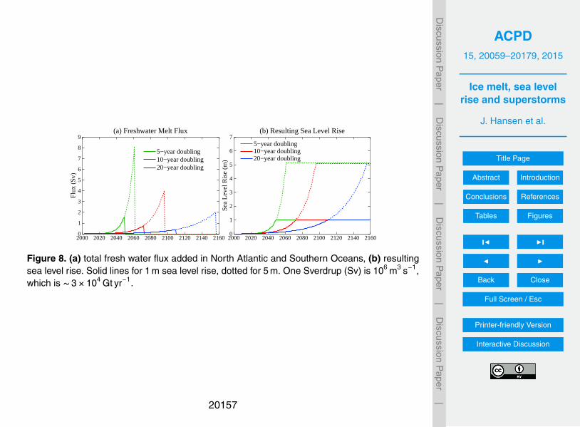
ACPD15, 20059–20179, 2015


J. Hansen et al.

Title Page



Tables Figures

J I

J I

Back Close

Full Screen / Esc



Discussion

Paper

|D

iscussionP

aper|

Discussion

Paper

|D

iscussionP

aper|

2000 2020 2040 2060 2080 2100 2120 2140 21600

1

2

3

4

5

6

7

8

9

5−year doubling10−year doubling20−year doubling

(a) Freshwater Melt Flux

Flu

x (S

v)

2000 2020 2040 2060 2080 2100 2120 2140 21600

1

2

3

4

5

6

75−year doubling10−year doubling20−year doubling

(b) Resulting Sea Level Rise

Sea

Lev

el R

ise

(m)

Figure 8. (a) total fresh water flux added in North Atlantic and Southern Oceans, (b) resultingsea level rise. Solid lines for 1 m sea level rise, dotted for 5 m. One Sverdrup (Sv) is 106 m3 s−1,which is ∼3×104 Gt yr−1.

20157





ACPD15, 20059–20179, 2015


J. Hansen et al.

Title Page



Tables Figures

J I

J I

Back Close

Full Screen / Esc



Discussion

Paper

|D

iscussionP

aper|

Discussion

Paper

|D

iscussionP

aper|

Figure 9. Surface air temperature relative to 1880–1920 in (a) 2065, (b) 2080, and (c) 2096.Top row is IPCC scenario A1B. Ice melt with 10 year doubling is added in other scenarios.

20158





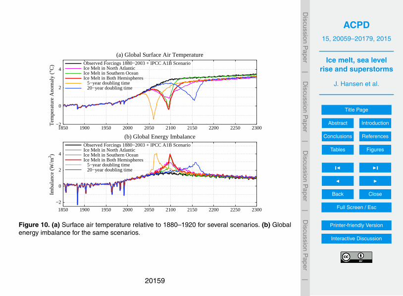
ACPD15, 20059–20179, 2015


J. Hansen et al.

Title Page



Tables Figures

J I

J I

Back Close

Full Screen / Esc



Discussion

Paper

|D

iscussionP

aper|

Discussion

Paper

|D

iscussionP

aper|

1850 1900 1950 2000 2050 2100 2150 2200 2250 2300−2

0

2

4Observed Forcings 1880−2003 + IPCC A1B ScenarioIce Melt in North AtlanticIce Melt in Southern OceanIce Melt in Both Hemispheres 5−year doubling time 20−year doubling time

(a) Global Surface Air TemperatureT

empe

ratu

re A

nom

aly

(°C)

1850 1900 1950 2000 2050 2100 2150 2200 2250 2300

−2

0

2

4

Observed Forcings 1880−2003 + IPCC A1B ScenarioIce Melt in North AtlanticIce Melt in Southern OceanIce Melt in Both Hemispheres 5−year doubling time 20−year doubling time

(b) Global Energy Imbalance

Imba

lanc

e (W

/m2 )

Figure 10. (a) Surface air temperature relative to 1880–1920 for several scenarios. (b) Globalenergy imbalance for the same scenarios.

20159





ACPD15, 20059–20179, 2015


J. Hansen et al.

Title Page



Tables Figures

J I

J I

Back Close

Full Screen / Esc



Discussion

Paper

|D

iscussionP

aper|

Discussion

Paper

|D

iscussionP

aper|

Figure 11. Change in 2078–2082, relative to 1880–1920, of the annual mean (a) planetaryenergy balance, (b) cloud cover, and (c) net energy into the ground, for the same four scenariosas in Fig. 9.

20160





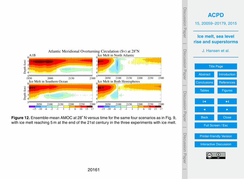
ACPD15, 20059–20179, 2015


J. Hansen et al.

Title Page



Tables Figures

J I

J I

Back Close

Full Screen / Esc



Discussion

Paper

|D

iscussionP

aper|

Discussion

Paper

|D

iscussionP

aper|

Figure 12. Ensemble-mean AMOC at 28◦ N versus time for the same four scenarios as in Fig. 9,with ice melt reaching 5 m at the end of the 21st century in the three experiments with ice melt.

20161





ACPD15, 20059–20179, 2015


J. Hansen et al.

Title Page



Tables Figures

J I

J I

Back Close

Full Screen / Esc



Discussion

Paper

|D

iscussionP

aper|

Discussion

Paper

|D

iscussionP

aper|

Figure 13. Change of seasonal mean (a) sea level pressure and (b) wind speed in 2078–2082relative to 1880–1920, and (c) the wind speed itself, all for the scenario with ice melt in bothhemispheres.

20162





ACPD15, 20059–20179, 2015


J. Hansen et al.

Title Page



Tables Figures

J I

J I

Back Close

Full Screen / Esc



Discussion

Paper

|D

iscussionP

aper|

Discussion

Paper

|D

iscussionP

aper|

Figure 14. Ensemble-mean AMOC at 28◦ N versus time for six pure freshwater forcing experi-ments.

20163





ACPD15, 20059–20179, 2015


J. Hansen et al.

Title Page



Tables Figures

J I

J I

Back Close

Full Screen / Esc



Discussion

Paper

|D

iscussionP

aper|

Discussion

Paper

|D

iscussionP

aper|

0 50 100 150 200 250 30011.5

12.0

12.5

13.0

13.5

14.0

0.5 m Sea Level Rise2.5 m Sea Level Rise

(a) Freshwater in North Atlantic

T (

°C)

Global Surface Air Temperature

0 50 100 150 200 250 30011.5

12.0

12.5

13.0

13.5

14.0


(b) Freshwater in Southern Ocean

Figure 15. Ensemble-mean global surface air temperature for experiments (years on x axis)with freshwater forcing in either the North Atlantic Ocean (left) or the Southern Ocean (right).

20164





ACPD15, 20059–20179, 2015


J. Hansen et al.

Title Page



Tables Figures

J I

J I

Back Close

Full Screen / Esc



Discussion

Paper

|D

iscussionP

aper|

Discussion

Paper

|D

iscussionP

aper|

Figure 16. Change of ocean temperature relative to control run due to freshwater input thatreaches 2.5 m of global sea level in a hemisphere (thus 5 m sea level rise in the bottom row).

20165





ACPD15, 20059–20179, 2015


J. Hansen et al.

Title Page



Tables Figures

J I

J I

Back Close

Full Screen / Esc



Discussion

Paper

|D

iscussionP

aper|

Discussion

Paper

|D

iscussionP

aper|

0 50 100 150 200 250 300 0

1

10

100


(a) Rate of Freshwater Input

Flu

x (T

t/yea

r)

0 50 100 150 200 250 300−7

−6

−5

−4

−3

−2


(b) SMOC (Mean Ocean Overturning at 72°S)

SM

OC

(S

v)

0 50 100 150 200 250 300

−1.4

−1.2

−1.0

−.8

−.6 0.5 m Sea Level Rise2.5 m Sea Level Rise

(c) Ocean Temperature at ~1 km Depth at 74°S

T (

°C)

0 50 100 150 200 250 300 0

2

4

6

8

10

12(d) Sea Ice Cover in Hemisphere of FW Input

Ice

Cov

er (

%)

Southern Hemisphere

Northern Hemisphere

Figure 17. (a) Freshwater input to Southern Ocean (1 Tt = 1000 km3 yr−1). (b, c, d) Simulatedoverturning strength (Sv) of AABW cell at 72◦ S, temperature at depth 1.13 km at 74◦ S, andhemispheric sea ice cover.

20166





ACPD15, 20059–20179, 2015


J. Hansen et al.

Title Page



Tables Figures

J I

J I

Back Close

Full Screen / Esc



Discussion

Paper

|D

iscussionP

aper|

Discussion

Paper

|D

iscussionP

aper|

1850 1900 1950 2000 2050 2100

−2

0

2

4

6 Greenhouse GasesTropospheric AerosolsStratospheric AerosolsSolar IrradianceLand Use

A1B Scenario

Effe

ctiv

e F

orci

ng (

W/m

2 )

(a)

1850 1900 1950 2000 2050 2100

−2

0

2

4

6 Greenhouse GasesTropospheric AerosolsStratospheric AerosolsSolar IrradianceLand Use

Modified Forcing Scenario

(c)

1850 1900 1950 2000 2050 2100

−2

0

2

4

6

Net Forcing

Effe

ctiv

e F

orci

ng (

W/m

2 ) (b)

1850 1900 1950 2000 2050 2100

−2

0

2

4

6

Net Forcing

(d)

Figure 18. Effective global climate forcings in our climate simulations relative to values in 1850.

20167





ACPD15, 20059–20179, 2015


J. Hansen et al.

Title Page



Tables Figures

J I

J I

Back Close

Full Screen / Esc



Discussion

Paper

|D

iscussionP

aper|

Discussion

Paper

|D

iscussionP

aper|

1850 1900 1950 2000 2050 2100−1

0

1

2

3A1B ScenarioA1B + Modified Forcings, Ice Melt to +1mA1B + Modified Forcings, Ice Melt to +3.8m

(a) Global Surface Air TemperatureT

empe

ratu

re A

nom

aly

(°C)

1850 1900 1950 2000 2050 2100

−2

0

2

A1B ScenarioA1B + Modified Forcings, Ice Melt to +1mA1B + Modified Forcings, Ice Melt to +3.8m

(b) Global Energy Imbalance

Imba

lanc

e (W

/m2 )

Figure 19. Surface air temperature change relative to 1880–1920 (a) and global energy imbal-ance (b) for the modified forcing scenario including cases with global ice melt allowed to reach1 and 3.8 m.

20168





ACPD15, 20059–20179, 2015


J. Hansen et al.

Title Page



Tables Figures

J I

J I

Back Close

Full Screen / Esc



Discussion

Paper

|D

iscussionP

aper|

Discussion

Paper

|D

iscussionP

aper|

Figure 20. Surface air temperature change relative to 1880–1920 in 2055–2060 with the mod-ified forcings.

20169





ACPD15, 20059–20179, 2015


J. Hansen et al.

Title Page



Tables Figures

J I

J I

Back Close

Full Screen / Esc



Discussion

Paper

|D

iscussionP

aper|

Discussion

Paper

|D

iscussionP

aper|

Figure 21. SMOC, ocean overturning strength at 72◦ S, including only the mean (Eularian)transport (Sect. 4.5). This is the average of a 5-member model ensemble for the modifiedforcing including advanced ice melt (720 Gt yr−1 from Antarctica in 2011) and 10 year doubling.

20170





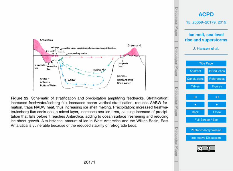
ACPD15, 20059–20179, 2015


J. Hansen et al.

Title Page



Tables Figures

J I

J I

Back Close

Full Screen / Esc



Discussion

Paper

|D

iscussionP

aper|

Discussion

Paper

|D

iscussionP

aper|

Figure 22. Schematic of stratification and precipitation amplifying feedbacks. Stratification:increased freshwater/iceberg flux increases ocean vertical stratification, reduces AABW for-mation, traps NADW heat, thus increasing ice shelf melting. Precipitation: increased freshwa-ter/iceberg flux cools ocean mixed layer, increases sea ice area, causing increase of precipi-tation that falls before it reaches Antarctica, adding to ocean surface freshening and reducingice sheet growth. A substantial amount of ice in West Antarctica and the Wilkes Basin, EastAntarctica is vulnerable because of the reduced stability of retrograde beds.

20171





ACPD15, 20059–20179, 2015


J. Hansen et al.

Title Page



Tables Figures

J I

J I

Back Close

Full Screen / Esc



Discussion

Paper

|D

iscussionP

aper|

Discussion

Paper

|D

iscussionP

aper|

Figure 23. Maximum mixed layer depth (in km, left, and % of ocean depth, right) in February(Northern Hemisphere) and August (Southern Hemisphere) using the mixed layer definition ofHeuze et al. (2013).

20172





ACPD15, 20059–20179, 2015


J. Hansen et al.

Title Page



Tables Figures

J I

J I

Back Close

Full Screen / Esc



Discussion

Paper

|D

iscussionP

aper|

Discussion

Paper

|D

iscussionP

aper|

−60

−30

0

30

60

60°N, Apr−May−Jun60°S, Oct−Nov−Dec

(a) Late Spring Insolation Anomaly at 60°N and 60°S

W/m

2

129.5 107.2 85.7 13.2121.1 98.376.9 5.8

−45

−40

−35

(b) Greenland δ18O

δ18O

(o / oo) H 10 9 8 7b7a 6 5 4 3 2 1

D−O 26 25 24.1 23.1 22 21 19 1715 13 11 9 7 5 3 2.1a 120 −45

−40

−35

δ18OCO2

(c) Antarctic δ18O and CO2

δ18O

(o / oo)

−50

−45

−40

200

250

300

350

400

CO

2 (p

pm)

300 400 500 600 700

CH4N2O

(d) CH4 and N2O Ice Core Composite

CH

4 (p

pb)

N2O

(pp

b)275250225200

−3

−2

−1

0

CO2 ForcingTotal GHG Forcing

(e) Greenhouse Gas Forcing

Fe

(W/m

2 )

←

3W/m2

in 2014

020406080100120140 −135

−90

−45

0

45

Grant et al.Lambeck et al.Ice Sheet Model

(f) Sea Level and Albedo Forcing

Time (kyr b2k)

RS

L (m

)

F (

W/m

2 )

0

−2

−4

6 5e d c b a 4 3 2 1 HMarine Isotope Stage

020406080100120140 −135

−90

−45

0

45

20173





ACPD15, 20059–20179, 2015


J. Hansen et al.

Title Page



Tables Figures

J I

J I

Back Close

Full Screen / Esc



Discussion

Paper

|D

iscussionP

aper|

Discussion

Paper

|D

iscussionP

aper|

Figure 24. (a) Late spring insolation anomalies relative to the mean for the past million years,(b) δ18Oice of composite Greenland ice cores (Rassmussen et al., 2014) with Heinrich events ofGuillevic et al. (2014), (c, d) δ18Oice of EDML Antarctic ice core (Ruth et al., 2007), multi-ice coreCO2, CH4, and N2O based on spline fit with 1000 year cut-off (Schilt et al., 2010), scales aresuch that CO2 and δ18O means coincide and standard deviations have the same magnitude,(e) GHG forcings from equations in Table 1 of Hansen et al. (2000), but with the CO2, CH4,and N2O forcings multiplied by factors 1.024, 1.60, and 1.074, respectively, to account for eachforcing’s “efficacy” (Hansen et al., 2005), with CH4 including factor 1.4 to account for indirecteffect on ozone and stratospheric water vapor, (f) sea level data from Grant et al. (2012) andLambeck et al. (2014) and ice sheet model results from de Boer et al. (2010). Marine isotopestage boundaries from Lisiecki and Raymo (2005). (b–e) are on AICC2012 time scale (Bazinet al., 2013),

20174





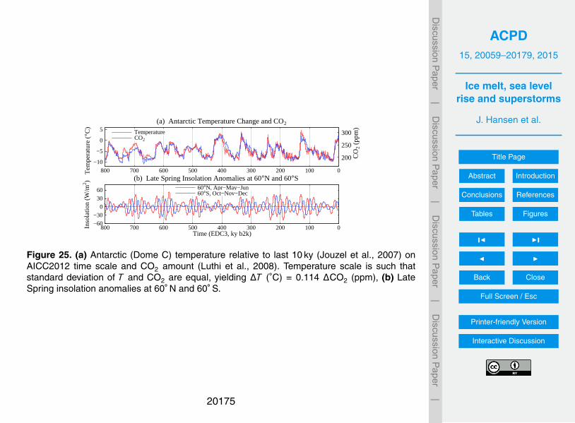
ACPD15, 20059–20179, 2015


J. Hansen et al.

Title Page



Tables Figures

J I

J I

Back Close

Full Screen / Esc



Discussion

Paper

|D

iscussionP

aper|

Discussion

Paper

|D

iscussionP

aper|

0100200300400500600700800

−10

−5

0

5 TemperatureCO2

(a) Antarctic Temperature Change and CO2

Tem

pera

ture

(°C)

200

250

300

CO

2 (p

pm)

0100200300400500600700800 −60 −30

0 30 60 60°N, Apr−May−Jun

60°S, Oct−Nov−Dec

(b) Late Spring Insolation Anomalies at 60°N and 60°S

Time (EDC3, ky b2k)

Inso

latio

n (W

/m2 )

Figure 25. (a) Antarctic (Dome C) temperature relative to last 10 ky (Jouzel et al., 2007) onAICC2012 time scale and CO2 amount (Luthi et al., 2008). Temperature scale is such thatstandard deviation of T and CO2 are equal, yielding ∆T (◦C) = 0.114 ∆CO2 (ppm), (b) LateSpring insolation anomalies at 60◦ N and 60◦ S.

20175





ACPD15, 20059–20179, 2015


J. Hansen et al.

Title Page



Tables Figures

J I

J I

Back Close

Full Screen / Esc



Discussion

Paper

|D

iscussionP

aper|

Discussion

Paper

|D

iscussionP

aper|

Figure 26. Simulated zonal mean temperature and eddy kinetic energy in 2078–2082 relativeto 1880–1920 base period for A1B scenario and A1B plus 2.5 m ice melt in each hemisphere(simulations of Sect. 3).

20176





ACPD15, 20059–20179, 2015


J. Hansen et al.

Title Page



Tables Figures

J I

J I

Back Close

Full Screen / Esc



Discussion

Paper

|D

iscussionP

aper|

Discussion

Paper

|D

iscussionP

aper|

1950 1975 2000 2025 2050 2075 2100

−6

−4

−2

0

2

(a) SMOC at 72°S, 2.1 km Depth

SM

OC

(S

v)

1950 1975 2000 2025 2050 2075 2100−2

0

2

4

6

ModelObservations

(b) Southern Hemispheic Mean Sea Ice Area Anomaly

mill

ion

km2

Figure 27. (a) SMOC, the global meridional overturning circulation at 72◦ S, in climate modelruns including freshwater injection around Antarctica at a rate 720 Gt yr−1 in 2011, increasingwith a 10 year doubling time, and half that amount around Greenland. SMOC diagnostic in-cludes only the mean (Eulerian) term. (b) Annual-mean Southern Hemisphere sea ice areaanomaly (relative to 1979–2000) in the five runs.

20177





ACPD15, 20059–20179, 2015


J. Hansen et al.

Title Page



Tables Figures

J I

J I

Back Close

Full Screen / Esc



Discussion

Paper

|D

iscussionP

aper|

Discussion

Paper

|D

iscussionP

aper|

February Sea Ice

1979-2015 Trend (%/yr)

2015 Area

Figure 28. Observed February sea ice extent (left); modeled and observed SST near Antarc-tica and global. Upper: 1979–2015 change based on local linear trend. Lower: 2015 anomalyrelative to 1951–1980. Sea ice data is update of Fetterer et al. (2002), temperature data isupdate of Hansen et al. (2010).

20178





ACPD15, 20059–20179, 2015


J. Hansen et al.

Title Page



Tables Figures

J I

J I

Back Close

Full Screen / Esc



Discussion

Paper

|D

iscussionP

aper|

Discussion

Paper

|D

iscussionP

aper|

1900 1920 1940 1960 1980 2000

0

50

100

150

200

Adjusted Tide Gauge DataSatellite Radar Altimetry

Global Mean Sea Level ChangeS

ea L

evel

Ano

mal

y (m

m)

0.6 mm/yr(1900−1930)

1.4 mm/yr(1930−1992)

3.3 mm/yr(1993−2015)

1900 1920 1940 1960 1980 2000

0

50

100

150

200

Figure 29. Sea level change based on satellite altimetry data (Nerem et al., 2010, updatedat http://sealevel.colorado.edu) and tide gauge data (Church and White, 2011) with the latterchange rate multiplied by 0.78, as required to yield a mean 1901–1990 change rate 1.2 mm yr−1

(Hay et al., 2015).

20179





http://sealevel.colorado.edu

ice melt, sea level rise and superstorms: evidence from paleoclimate

Documents