ice cloud retrievals and analysis with the compact...
TRANSCRIPT
Ice Cloud Retrievals and Analysis with the CompactScanning Submillimeter Imaging Radiometer and
the Cloud Radar System during CRYSTAL-FACE 1
K. Franklin Evans 2
Program in Atmospheric and Oceanic Sciences, University ofColoradoBoulder, Colorado
James R. Wang, Paul E. Racette, Gerald HeymsfieldNASA Goddard Spaceflight Center
Greenbelt, Maryland
Lihua LiUniversity of Maryland Baltimore County, Baltimore, Maryland
November 17, 2004
1Accepted by the Journal of Applied Meteorology2Corresponding author address: Dr. K. Franklin Evans, University of Colorado, 311 UCB, Boulder,
80309-0311. Email:[email protected]

Abstract
Submillimeter-wave radiometry is a new technique for determining ice water path (IWP) andparticle size in upper tropospheric ice clouds. The first brightness temperatures images of iceclouds above 340 GHz were measured by the Compact Scanning Submillimeter Imaging Ra-diometer (CoSSIR) during the CRYSTAL-FACE campaign in July2002. CoSSIR operated with12 channels from receivers at 183, 220, 380, 487, and 640 GHz.CoSSIR and the nadir viewing94 GHz Cloud Radar System (CRS) flew on the NASA ER-2 airplane based out of Key West,Florida. A qualitative comparison of the CoSSIR brightnesstemperatures demonstrates that thesubmillimeter-wave frequencies are more sensitive to anvil ice cloud particles than the lower fre-quencies. A Bayesian algorithm, with a priori microphysical information from in situ cloud probes,is used to retrieve IWP and median mass equivalent sphere particle diameter (Dme). Microwavescattering properties of random aggregates of plates and aggregates of frozen droplets are com-puted with the discrete dipole approximation (DDA) and an effective medium approximation tunedto DDA results. As a test of the retrievals, the vertically integrated 94 GHz radar backscattering isalso retrieved from the CoSSIR data and compared to that measured by the CRS. The integratedbackscattering typically agrees within 1 to 2 dB for IWP from1000 to 10,000 g/m
�, and while the
disagreement increases for smaller IWP, it is typically within the Bayesian error bars. Retrievalsmade with only the three 183 GHz and one 220 GHz channels are generally as good or better thanthose including 380
�6.2 and 640 GHz because the CoSSIR submillimeter-wave channels were
much noisier than expected. An algorithm to retrieve profiles of ice water content and Dme fromCRS and CoSSIR data was developed. This Bayesian algorithm also retrieves the coefficients ofan IWC - radar reflectivity power law relation and could be used to evaluate radar only ice cloudretrieval algorithms.

1. Introduction
There are no methods for accurate global remote sensing of ice cloud mass for climate studies(Wielicki et al., 1995). Global measurements of verticallyintegrated cloud ice mass (ice waterpath or IWP) are important for evaluating climate model parameterizations and studying the uppertropospheric water budget. Visible and infrared satelliteremote sensing techniques for ice clouds(e.g. Rossow and Schiffer, 1999; Stubenrauch et al., 1999) have poor accuracy for high IWP clouds,which contain much of the total cloud ice mass. Thermal infrared methods saturate for moderateoptical depth and can only determine particle size (and hence IWP) for effective radius below about50 �m. Solar reflection methods can’t distinguish ice from underlying water cloud optical depth,can’t measure thinner clouds over bright surfaces, and retrieve particle sizes only near cloud top foroptically thicker clouds, resulting in biased IWP retrievals. Millimeter-wave radar backscatteringfrom CloudSat (Stephens et al., 2002), when combined with visible reflectance measurements, willimprove IWP retrieval accuracy, but the radar’s nadir view provides coverage that is too sparse toobtain a global climatology of cloud ice mass with regional-scale resolution.
Theoretical studies (Gasiewski, 1992; Evans and Stephens,1995b; Evans et al., 1998) havesuggested that millimeter-wave and submillimeter-wave radiometry has the potential for accurateretrievals of cloud IWP and characteristic ice particle size. The technology of submillimeter-waveradiometry has lagged the theory, and only recently have thefirst submillimeter measurementsof ice clouds been made from aircraft. The Far InfraRed Sensor for Cirrus (FIRSC), which is aFourier Transform Spectrometer with a cryogenic bolometerdetector (Vanek et al., 2001), mademeasurements from 300 to above 1000 GHz during several campaigns. The sensitivity of FIRSC’sbolometric detector precludes cross-track scanning and the brightness temperature noise is high be-low about 800 GHz. The Submillimeter-Wave Cloud Ice Radiometer developed at the Jet Propul-sion Laboratory (Evans et al., 2002) has heterodyne receivers at 183, 325, 448, and 643 GHz, buthas not yet been flown. The Millimeter-wave Imaging Radiometer (MIR) (Racette et al., 1996)had receivers at 89, 150, 183, and 220 GHz. Several groups have developed cloud IWP retrievalalgorithms for MIR data at 89, 150, and 220 GHz (Liu and Curry,2000; Deeter and Evans, 2000;Weng and Grody, 2000). A 340 GHz channel was later added to MIR, and significant brightnesstemperature depressions were observed from Arctic cirrus (Wang et al., 2001).
The Compact Scanning Submillimeter Imaging Radiometer (CoSSIR) is a new instrument with15 channels from 183 to 640 GHz. CoSSIR flew for the first time onthe NASA ER-2 aircraft duringthe CRYSTAL-FACE deployment out of Key West, Florida in July2002. One of the objectives ofCRYSTAL-FACE was the improvement and validation of remote sensing methods for near-tropicalconvective anvil ice clouds. The 94 GHz nadir viewing Cloud Radar System (CRS) flew with CoS-SIR on the ER-2. In this paper we describe CoSSIR and show examples of millimeter-wave andsubmillimeter-wave brightness temperature depressions associated with convective anvils in thesouth Florida region. We describe the retrieval of ice waterpath and median volume equivalentsphere diameter (� � �), using a Bayesian algorithm with updated prior information on ice cloudmicrophysics. The appendices describe the in situ ice particle size distribution analysis and theparticle shape modeling that are used in the prior distribution for the retrieval. Retrievals fromCoSSIR of integrated radar reflectivity are compared with CRS data to evaluate the CoSSIR re-trievals. Lastly, a new algorithm is presented to retrieve profiles of ice water content (IWC) and� � � from the combination of CoSSIR and CRS data.
1

2. Data
During the month of July 2002, a major field campaign, the Cirrus Regional Study of TropicalAnvils and Cirrus Layers – Florida Area Cirrus Experiment (CRYSTAL-FACE), was conducted byNASA over the region surrounding Florida. Six aircraft equipped with a variety of remote sensinginstruments and in-situ probes participated in this campaign; all of these aircraft were stationed inKey West, Florida. The NASA ER-2 aircraft was one of the six and was equipped with a suite ofhighly sophisticated remote sensors including the CoSSIR and the 94 GHz Cloud Radar System(CRS) (Li et al., 2004) that measures radar reflectivity profiles of cloud particles.
The CoSSIR is a new, total-power radiometer that has a total of 6 receivers and 15 chan-nels. Twelve channels are horizontally polarized at the frequencies of 183.3�1.0, 183.3�3.0,183.3�6.6, 220�2.5, 380.2�0.8, 380.2�1.8, 380.2�3.3, 380.2�6.2, 487.25�0.8, 487.25�1.2,487.25�3.3, and 640�2.5 GHz, and 3 vertically polarized channels at 487.25�0.8, 487.25�1.2,487.25�3.3 (see Table 1). All six heterodyne receivers use highly integrated subharmonicallypumped Schottky-barrier mixers. The local oscillators usethermally stabilized Gunn diode oscil-lators followed by varactor-diode multiplier chains (except the 183 receiver which just uses a Gunndiode oscillator). Images are generated by rotating the receiver scanhead assembly on a dual-axesgimbals which can be programmed to perform across-track scans as well as conical scans at a fixedincidence angle. During CRYSTAL-FACE it was programmed in across-track scan mode so thatcoincident measurements with the CRS and MODIS Airborne Simulator could be made. The 3 dBbeamwidth is about 4 degrees and is frequency independent; at the ER-2 aircraft cruising altitudeof about 20 km, the footprint at a typical ice cloud altitude of 10 km is 600 m. The scan cycle ofCoSSIR is 4.6 s. During each scan cycle the antennas view an effective angular swath of�50�(from nadir) for 2.6 s, as well as hot (maintained at about 328K) and cold (at an ambient tempera-ture of about 255 K) calibration targets for 0.5 s each. Thesecalibration targets are closely coupledto the antennas and their temperatures are each measured by 8resistive temperature sensors towithin 0.1 K. The calibration accuracy of the CoSSIR measured scene brightness temperatures(Tb) is estimated to be within�2 K in the Tb range of 100 to 300 K.
Table 1 gives a comparison of the calculated and measured noise-equivalent-temperature dif-ference (NE�T) for all the working channels; the 380.2�0.8 GHz channel and the 487 GHz hor-izontal polarization receiver did not function during the entire deployment. Clearly the measuredvalues of NE�T are 2 to 10 times higher than the calculated values. The excess noise is attributedto inadequate grounding and the analog-to-digital conversion. A modification to the signal con-ditioning and grounding is required to eliminate this excess noise source and improve the sensorperformance. In addition, the local oscillator for the 380 GHz receiver exhibited instability whichprevented those channels from being used for sounding.
Table 2 lists a summary of the CoSSIR flights for this deployment. There were a total of 11science flights in Florida and two transit flights between NASA Dryden Flight Research Center atEdwards Air Base, California and Key West, Florida in July 2002. CoSSIR experienced a motioncontrol problem for six science flights from July 9 through 23, which was resolved by adjustingthe gain of the motion control feedback. Towards the end of the tenth science flight on July 28, thepilot inadvertently turned off the power to CoSSIR before decent and the whole system was cold-soaked after landing. Only the four lowest frequency channels (183.3 and 220 GHz) and the 640GHz channel remained operational after this incident. The calibrated CoSSIR data sets along nadirwere placed in the CRYSTAL-FACE archive (athttp://espoarchive.nasa.gov/). The
2

Table 1: CoSSIR channel characteristics.
Channel Center Bandwidth System NET NET�Frequency Temperature (calculated) (measured)
(GHz) (GHz) (GHz) (K) (K) (K)
183.3�1.0 1.0 0.5 2500 0.55 0.90183.3�3.0 3.0 1.0 1390 0.23 0.61183.3�6.6 6.6 1.5 1050 0.15 0.75
220 2.5 3.0 1760 0.16 0.84380.2�0.8 0.75 0.7 3460 0.63 NA380.2�1.8 1.80 1.0 8440 1.23 4.01380.2�3.3 3.35 1.7 4820 0.55 4.25380.2�6.2 6.20 3.6 6670 0.52 4.99487.25�0.8 0.68 0.35 4650 1.17 2.57487.25�1.2 1.19 0.48 3890 0.85 1.66487.25�3.3 3.04 2.93 4600 0.40 2.05
640 2.5 3.0 16000 1.33 4.90Calculated values based on receiver system temperature measured in thelaboratory and 50 msec integration time.�Measured from the calibration tar-get data on the July 1 flight with the same integration time.
imagery data sets are deemed too large for archiving; they will be made available by contactingone of us (e.g., [email protected]).
The CRS is a new instrument operating at 94 GHz frequency thatwas built and first flown inCRYSTAL-FACE. It is a Doppler, polarimetric radar developed for autonomous operation on theER-2 aircraft and ground operation (Li et al., 2004). Its antenna beamwidth and gain are 0.6 x0.8 and 46.4 dB, respectively. It has a noise figure of 10.0 dB and its receiver bandwidth can be variedbetween 1, 2, and 4 MHz. The system transmits power in either vertical (V) or horizontal (H) po-larization, and receives backscatter power in both V and H polarization at the nadir direction. Thedataset used here has a measured sensitivity of -29 dBZe at 10km range, 150 m range resolution,and 1 second averaging. The calibration of the CRS was conducted by two different methods. Thefirst one was an inter-comparison of the concurrent ground-based measurements for similar cloudvolumes between the CRS and the ground-based 95 GHz Cloud Profiling Radar System (CPRS)owned by the University of Massachusetts (Sekelsky and McIntosh, 1996) and well maintainedand calibrated over the past decade. This comparison demonstrated consistency between the twoinstruments to better than 1 dB (Li et al., 2004). The second method was to use the ocean sur-face (Durden et al., 1994) by estimating scattering cross section of the surface return�� at a lowincidence angle and with quasi-specular scattering theory(Valenzuela, 1978). The ER-2 aircraftdropsondes provided temperature, pressure, relative humidity, and near-surface wind conditionsthat were required to take into account the effect of atmospheric absorption by water vapor andoxygen, as well as the calculations of�� . The analysis showed that the calculated�� agreed withthe other CRS calibration results. The details of the systemdescriptions, sensitivity, and calibra-
3

Table 2: Summary of CoSSIR science flights during CRYSTAL-FACE (2002).
Flight Date Status Receivers working
Transit July 1 Successful 183.3, 220, 380, 487 and 640 GHz1 July 3 Successful 183.3, 220, 380, and 640 GHz2 July 7 Successful 183.3, 220, 380, and 640 GHz3 July 9 Failed4 July 11 Failed5 July 13 Failed6 July 16 Failed7 July 19 Failed8 July 23 Failed9 July 26 Successful 183.3, 220, 380, and 640 GHz10 July 28 Successful 183.3, 220, 380, and 640 GHz11 July 29 Successful 183.3, 220, and 640 GHz
Transit July 30 Successful 183.3, 220, and 640 GHz
tion can be found in Li et al. (2004). The CRS successfully collected scientific data from all theflights listed in Table 2.
Figures 1, 2, and 3 provide a glimpse of data acquired by the CoSSIR and CRS during CRYSTAL-FACE. Figure 1 shows an example of pseudo-color image of brightness temperatures (��) forseveral selected CoSSIR channels from a segment of a transitflight from NASA Dryden FlightResearch Center to Key West, Florida on July 1, 2002. The swath of each image is about 45 kmacross at the ground (much less for high clouds) and the segment covers a distance of about 600 km.Two strong cells of ice clouds can be found near the times of 1952 UTC and 2010 UTC; a weakcell is also spotted at 2032 UTC. These cells clearly demonstrate that ice clouds strongly scattersubmillimeter-wave radiation and that the�� depressions are generally larger at higher frequencies.Notice that the effect of water vapor absorption causes a large range in the� � values from the three183.3 GHz channels.
Figure 2 gives a comparison of the along-nadir� � values from some selected CoSSIR chan-nels with the concurrent radar reflectivity profiles�� measured by the CRS. The time interval ofthe plot covers about the top half of the images in Figure 1. The two large� � depressions near1952 UTC and 2010 UTC identified with the ice clouds from the�� images in Figure 1 are clearlyassociated with the high CRS�� values. The�� depression from the isolated high cloud around2006 UTC is much greater at 640 GHz than 220 GHz. Another smaller 640 GHz� � depressionnear 2016 UTC not apparent in Figure 1 finds its correspondence in CRS�� profile as well. Addi-tionally, the higher-frequency channels generally show�� depressions over a greater distance thanthe lower frequency channels. For example, the�� values around 1958 UTC from the 183.3�6.6and 220 GHz channels are already recovered to their clear skyvalues, while those from the 640GHz channel remain slightly depressed due to the presence ofhigh clouds detected by the CRS.This demonstrates the increased sensitivity of the 640 GHz channel to high and thin clouds, whichcomplements the lower frequencies’ sensitivity to larger particles and lower altitudes. For exam-ple, around 2000 the 220 GHz channel shows a double-dip structure while the 640 GHz channel
4

Figure 1: Example brightness temperature images from 10 of CoSSIR’s channels.
5

has only the second dip. The radar profile indicates that the 640 GHz channel misses the first cellbecause it is at a lower altitude, where water vapor absorption blocks the 640 GHz signal.
Another important feature displayed by the CoSSIR data is the non-linear behavior of the��relation between high and low frequencies, shown by the scatter plot in Fig. 3 for the 640 and 220GHz channels. In the higher�� range with small depressions, the 640 GHz� � decrease is steeperthan the 220 GHz decrease, implying a higher sensitivity of 640 GHz to thinner ice clouds. Thishigher sensitivity of the higher frequency implies clouds with a smaller median mass diameter(� � �) particles (see Figure 3 of Wang et al. (1998)). In the lower�� range corresponding tolarger depressions, the 640 GHz depression is less than thatat 220 GHz, implying larger� � �and generally thick clouds over regions of precipitation. The small population of points below theslanted line are from times when the 640 GHz��s were drifting unphysically. The points inside
Figure 2: Nadir CoSSIR brightness temperatures and corresponding CRS radar reflectivity.
6

the ellipse are from lower altitude ice clouds (as verified byCRS data), for which the water vaporabsorption reduces the� � depression at 640 GHz.
3. Vertically integrated ice cloud retrieval algorithm
A Monte Carlo Bayesian integration algorithm (Evans et al.,2002) is used to retrieve ice cloudIWP and� � � from the CoSSIR brightness temperatures. The Monte Carlo integration is overstate vectors� of cloud and atmosphere parameters. A priori information onthe temperatureand water vapor profile and ice cloud geometry and microphysics is introduced by distributingthe vectors randomly according to a prior probability density function (pdf),!" #� $. A radiative
120 140 160 180 200 220 240 260 280 300220 GHz Brightness Temperature (K)
120
140
160
180
200
220
240
260
280
300
640
GH
zB
right
ness
Tem
pera
ture
(K)
..
.......
... ..................
........
.
.........
.....
.
.
.
...... .
.....................
...................
.......
...
.
.................................
.
.......
.
.......
.
.......................
.
...........................................................................
...
..........
............................
.
.
.....................................
........
...........................................
.....
....
........................
..
................................................
.........
....
.......
.
.........
...............
.............................
............
..............
...
......
.....................................
....
...........
......
...............
.
...
.....................................................
...................
.......................
..................
...
.
.
......
.
.....
............
..........
....
....... .
........
.
...
.
......................
.
.................................
.
... ....
.
...
.
...
....
............
..........................................
............
...............
.......
...
..
.
.
..
...
.....
.
.........
.
.
..................
......
.
....................................
.
.
.........
.
..
.........
.
.
.....
.
...........
.
.
.
...............
...
......
.
..
....... ............................... .....................................................
...................................
..................
................
......
...
.......
...............................
............
.....................
...........
.
...
..
................
.
...................
.
....
. ...........
..............
........
.
.......
... ..........
..
......
.
..... .
.....
..... . ..
..
...................................
.....
..... . . .
.......................................................
.
...........
.......
.
.......................
.......
........
. ...................................
..
.
..........................
.......................
.
.
.........
......
...............
.....................................
........
...........
.
...
.
................
..................................
.......
..
.
...
..
....
......
.
.......................................
..
....................
.
.
.............
..............................
........
......... .....
...
..
..
.......
...
.. ....
.
................
.. .. . ..
.
...........
. . ... ...........................
.
....
....
.
...
..
..... .....
.
.......................
.
...........................
...........................
..
...
........................
.
.........................................
................
..............
.................
.................................
.................................
.
.
.....
...
....
..
.........
.
... .
. .
..
..
.
... .........
..
.
.. .
.
.
.
.
..
.....
.
..... ..
..
.. .
.
..
......
...
.....
...........
.
.
....
.
............
.
... .
.. .
.. .
.. .
..
..
.
.
...................................
.
...........................................
.
...
.....
.
.......... .
..................................................................................................................................................................
......................
.
.......
..
.
....
..
..
......................
....
. ......
..
......
. .... .
. ......
.....................
..
.
.............................
................
.
...
.
.
....................................
.............................................................................
.
.
..
..................................
..
.
.. ...
....
......
.....
.
........
.. .
..
. .......
.
............
...
.
.
.....
......
....
.
.
..............
..
.....
.... . ..
.
..
....
.
.
.
.
..
...
. . .. .
...
..
.........................
...................... ..............
..............
...
....
...
....
....
.
..... ................................
..........................
....................
.
...........
.
.
..
.
..
.
... ..
......
.
........
......
.
.
.
.
.....
....
.......................
........................................
...............
..
....................
.
.
.
.
..
.....
....................
.
.....
..
.......................
.
.
...
.
....
..
..............
........
...............................................
.............
........................
...
.
...........
...... ..........
.
............
........................................... .....................
....................
.
.................
..
................
.
.
..................
.......
. ............
.........
.............
.
..
...
...
............
...
.
.............
...
.....................
.............................
........
........... .
.............................................
...
.....................
.
....
.....
...
...
.........
........
.
..........................
..... .
. ....................
.
.........
................
.
...........................
.
.
.....................................................
............................
...
...
.
.
...
...
.................................
........................
.
.
.......
. .
......
..
. .. .
.
.
..
....
...
..
.. ......
........
.....
.......
.
..
....
.
..
..
... .. .
.
. ... ..
..
.
. .
. ........
..................................................................
.
.....
.
...
................
.
.......
....
...
.. . .......
.
..... .
..
................
..................................... ..
..
....
..
.
...............
.
.....
.
.
. .....
.. ........
.............
.
.
.......
.....
.
...
.
.. .
.
..
.
. .....
...
.
..
..
..
.
....
.
.
.
.
.
..
....
.
..
.
. ....................................
.............
. ................................ ......................
..............................................
.
..
......
............
.............
......
....
..
....
...
..
.....
......
....
. .........
...
. ...
..
....
.......
........ ......
........
..
....
...
.
.
......
........
...........
..........
...............
......
.
..
....
.
...
... .
. ....
.
... ..........
. . .... .
.. . .
.... . . .
....
......
.............
.
..
.
.....
.
...
.
...
.
.
..
.
......................
..........
.
....
. ....
.
....
...
.......................
.................
....
.
....................
......................
..
...
.
...
... ....
.. ..
. ...... ....... . .
.
..
.
..
.
..
...
.
.
.
. .
.. .
.
..
. .. ... .
.....
. .. .
...
.....
...........
.
.....
.
.... ..
.
. .. .. . .
.
....
...
...
..
.
....
.. ..
..
.. . .. ..
. .
... . .
.....
................
......
.......
.....
......
.....
.... .. . ..
... .
. ..
. .....
...
........
..
.
..
.
. ...................
.....................................
....
..................
.........................
.....
..............
..............
...
....
...
.....
.
......
....
.
.
....
......
..
.
..... .
.
...
..
... .
.
. .
... .. .
. .........
..........
..
... . .
. ... ..........
.
....
.
.....
.
.
...
......
.......
.....
. .
. ..
.
.
..
......
....
.....................
.
.
........
......
.
.
.
.
..
...... .....
... .
.
.... .................... ........
...
.
... ......
...
....
........
........
.
..
....
...
.
.
.
.
.
.
.
.
..
...
..
..
..............
..
........
.........
..
.......
.
....
..........
.................
................
.......
...
................
....
.
.
.....
.
.....
..................
..........
..................
.
...
...
........
.
.
.
.
.........................
....
.
................... ..............
...
.... ...............
.................
.
.................................
.................................
........
...........................
............
.........
.....
.
.......................
.............................
.
........
..............................
.
.....................
...........................................................
.
.......
.........
..
........... .....................
..
.
............
..
.
...
.
.
.
.
.
..
...
.
......
....
.......
..
........
.
..
...
.
..........
.... .....
...
.....................
.
...
..........
...........................
.
..
......................
...........
.........
....
...................
.
..
.
...
.
...............
.
.........
...
..........................
..........
.
..
.
......
..............
..
....
.
............
........................
.
..
..
.
........
.
.
....
..............................................
.......................
..
.........
...
.......
.. ................... .
.
..
.........
..........................
.................................................
.
.........
...............................
.........................
............
............................................
....
.............................................
.
..............................
.......
..
.
.........................
.............
......
..
........
......
...
....
...
.
..........
...... .....
.
..
..
.
. .
. ..........................................
..
...
..............
..
.
......
.
.............
......
..............
.
.......................
...............................
....
.......
....
..............
..
....................
.
...
.
........................ ................
..............
..
.................
...
.
.....
. ...
..................
... ... .. .
... ........... ..........
.. .
..
.
..
......
.................................................
...
.
..
..
.......
.
....
..............
.............
..
...
..
....
.....
...
..
.
.....
.......
.... ..
...............
.. ..
.....
. . . .. .
. .
.
................
.............
....
....
. ..........
..
.
.....
..............
..........
......................
..........
.......................
...
.
.
.
.....
...
...
.
......
......
......
........
.
.. .
.... .... ..
......
.... . .
.. .
.
.......
..
......................
.
.
.......
.
..
.
..........................
.....
...
.................
...
..................
.........................
..............
...
.
.....
...
..
..........
...
.......
.............
..
........
..
..
......
........
. ... . . .
. .
. .. .
.
. ... .
.
.
.....................
. .........
.
.........
.
.
...
...........
..
......
.........
.
...........................................
....
.
.
..
.
.........
.....
...............
.
.....
......
.
.
.........
...
.. .. .
.. .
. . .. ....
..... .....
....................................
.......
.
.
...
.....................
.........................................................
........
...
................
...............
......
...
...
......
..
.....
....
.
..
....
.....
.....
....
.
........
..... ..
......... .
.. .. . . ... .. .
.. .
.. .
.
. .
............
................
..............
..................................
................
.....
.
...
.....
...
........
....
..
............... .................. ...
........
.........
.
........................
.
.
...............
.........................................
..........
.
....
.
...
............
.
..
....
...................................
.............
.
.
..
.
........
.............
...............
.......
..
......
...
........
.......
..
........................
.
.
....... .
....
...........
.
...
.
...
....
.........
.....
.....
...
. ......
.
..................................
Figure 3: Scatterplot of nadir CoSSIR 640 and 220 GHz brightness temperatures from July 3, 28,and 29. See text for discussion of points delineated by the line and ellipse.
7
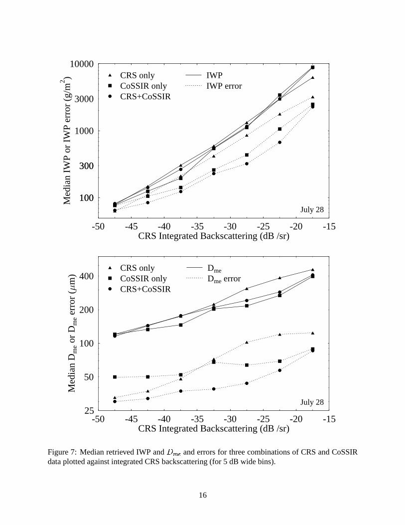
transfer model simulates CoSSIR brightness temperatures% &'( )* (for the + ’th channel) from thecloud and atmosphere profile represented by,'. A retrieval for the CoSSIR observed brigthnesstemperatures,%-.& )* (with rms uncertainty of/* ), is performed by computing the mean state vectorover the posterior pdf from Bayes theorem. Assuming a normally distributed likelihood functionfor the observations given the state vector, the retrieved state is
,012 3 4 ' , ' 567 89 :; <;' =4 ' 567 89 :; <;' = , ' >?@A BC D, E (1)
where< ;is the usual normalized measure of the disagreement betweenthe observed and simulated
brightness temperature vectors,
<;' 3 FG* H :I% -.& )* 9 % &'( )* D, ' EJ;/ ;* (2)
An estimate of the uncertainty in the retrieval is given by the standard deviation around the meanvector,
/ ;K 3 4 ' D,' 9 ,012 E; 567 89 :; <;' =4 ' 56 7 89 :; <;' = , ' >?@A BC D, E (3)
For efficiency the simulated brightness temperatures for each Monte Carlo vector (,') are precom-puted with a radiative transfer model and stored with the desired retrieval parameters (e.g. IWPandL ( 1) in a file called the retrieval database. The database used here hasMNO cases in it.
Several minor improvements have been made to the Bayesian ice cloud retrieval algorithmdescribed in Evans et al. (2002). Missing channels are dealtwith by simply setting that channel’s/* to 1000 times the normal value. The algorithm requires a minimum number of database points(25 in the retrievals below) within a specified< ;
threshold, here set toP Q R S P , whereP isthe number of channels in the retrieval. This choice of the<;
threshold is guided by noting thatfor Gaussian measurement noise andP T M, the expected value of<;
is P and the standarddeviation of<;
is S UP . If there are fewer than the required number of points withinthis thresholddue to the finite number of points in the retrieval database, then a larger<;
range is considered byeffectively increasing all the/* ’s in steps of a factor ofS U until the minimum number of points isreached. This implies that there is a source of retrieval error due to the finite database size. Sincethe points in the database are distributed according to the prior pdf, there are few cases with highIWP. The database generation procedure has the option of rejecting low IWP cases according to anexponential probability distribution in IWP and increasing the weight of the remaining cases so thatthe high IWP enriched retrieval database is statistically equivalent to the prior pdf. This procedureimproves the problem of not having enough database points within the required< ;
threshold forhigher IWP.
Generation of the database of atmospheric parameters and corresponding brightness temper-atures is the key element of the Bayesian algorithm. The firststep in generating the database isto create random profiles of temperature, water vapor, liquid and ice cloud properties, and surfaceemissivity. The distribution of these parameters is the a priori information in the retrieval, so it isimportant that the profiles are realistic and completely cover the possible parameter range. The re-trieval does depend on the prior distribution, but the variation in the retrieved parameters due to the
8

a priori assumptions is small compared to the retrieved error bars (as long as the prior distributioncontains a wide range of atmospheric states and the measurements provide useful information).
The retrieval database temperature and relative humidity profiles are generated with appropriatestatistics and vertical correlations using principal component analysis. The principal componentsare calculated from 25 radiosonde profiles on July 3, 7, 9, 21,28, 29 obtained from the MiamiNational Weather Service and the PNNL Atmospheric Remote Sensing Laboratory (PARSL) atthe west coast ground site. Twenty principal components, which explain 99.8% of the variance intemperature and relative humidity, are used. Heights abovethe highest radiosonde level and thefixed ozone profile are obtained from a standard tropical atmosphere. The mean relative humidityprofile in the generation process (not the output stochasticprofile) is set to ice saturation for thecloudy levels.
This retrieval database is made with single layer clouds, which may be ice, mixed phase, oreven pure liquid depending (stochastically) on temperature. The cloud geometry statistics areobtained from over 1400 cloudy CRS profiles on four flights, where the thickest cloud layer withtop height above 9.5 km is chosen from each profile. The top height is Gaussian distributed witha mean of 12.7 km and and standard deviation of 1.2 km. The cloud thickness is exponentiallydistributed with a mean of 5.0 km.
The microphysical properties of the ice clouds in the retrieval database are based on CRYSTAL-FACE data from in situ cloud probes on the Citation aircraft.The results of this analysis (describedin appendix A) are the joint statistics of temperature, IWC,andV W X as summarized by the meanvector and covariance matrix of temperature,YZ(IWC), andYZ [V W X \. The randomly generated icecloud heights and thicknesses are used to index into the random temperature profiles to get cloudtop and bottom temperatures. Given the top and bottom temperature, the IWC andV W X at the topand bottom of the cloud are generated randomly from the bivariate log-normal distribution. TheV W X varies linearly with height inside the cloud, while the IWC varies as a power law inV W X. Thebottom IWC andV W X are required to be larger than cloud top values.
Ice particle shape and size distribution width are error sources in the ice cloud retrievals. Theconstruction of random aggregate particles based loosely on Cloud Particle Imager pictures andthe simulation of CoSSIR and CRS scattering properties for size distributions of these particles isdescribed in appendix B. For each cloud a single particle shape is selected from the five modeledshapes (low-density spherical snow, aggregates of frozen droplets, two varieties of aggregates ofhexagonal plates, and aggregates of plates and hexagonal columns). The width of the ice particlegamma size distribution is also randomly chosen for each cloud from three widths.
The surface has a small contribution at 220 GHz for the drier stochastic atmospheres (the220 GHz transmission for the mean atmosphere is only 4.4%). Even the driest atmospheres haveessentially no transmission at the other CoSSIR frequencies. The surface emissivity is Gaussiandistributed with a mean of 0.93 and a standard deviation of 0.03 (representing a land surface). Thesurface temperature is obtained from the random atmospheretemperature at zero height.
The second part of generating the retrieval database is to simulate the CoSSIR and CRS obser-vations with a radiative transfer model. A fast Eddington second approximation method is used.The microwave radiances are simulated for a nadir viewing angle. For efficiency the monochro-matic absorption profiles for an input atmosphere are interpolated in temperature and water vaporfrom reference profiles calculated with LBLRTM version 8.3.Double sideband brightness tem-peratures are calculated with two monochromatic radiativetransfer computations. The tabulatedsingle scattering properties for the ice particles are computed as described in appendix B.
9

In addition to the simulated CoSSIR brightness temperatures, the retrieval database has twosimulated 94 GHz CRS observables: integrated attenuated backscattering (]^) and the mean backscat-tering weighted height (_^). The integrated attenuated backscattering is defined by
]^ ` a bcb de^fgh i_ jkl mnop qb rs_ ` a bcb d
e tgf u ivwxy jkl mnop qb rs_ z (4)
and the mean backscattering weighted height is defined by
_^ ` { bcb d e^fgh i_ j_ mnop qb rs_{ bcb d e ^fgh i_ j mnop qb rs_ z (5)
wheree^fgh i_ j is the volume backscattering coefficient,etgf is the volume scattering coefficient,u ivwxyj is the phase function evaluated in the backscattering direction, mnop qb r is the two wayattenuation along the optical path| i_ j, and _} to _o is the height range. The height range usedhere is 4.5 to 17 km, or all cloudy levels above the freezing level. Although not in common use inradar meteorology, integrated backscattering is a naturalmeasure in radiative transfer and is usedin lidar remote sensing. The units of integrated backscattering are stern}. The radar observablesin the database are used 1) to retrieve]^ from CoSSIR data to compare with CRS data, and 2) toperform IWP and~ � � retrievals with the combination of CoSSIR and CRS data.
4. CoSSIR and CRS vertically integrated ice cloud retrievals and analysis
To perform the Bayesian ice cloud retrievals from CoSSIR measurements, the rms uncertainties(e� ) must be determined for each channel during each flight. Onlythe nadir viewing CoSSIRbrightness temperatures for roll angles less than 8y are used. The “noise” of the CoSSIR�^s aredetermined by calculating the standard deviation for clearsky segments of the flights. Clear skyis defined as those pixels for which the MODIS Airborne Simulator (MAS) 11.0�m brightnesstemperature is above 295 K. This method for estimating thee ’s assumes most of the variabilityis instrumental, not due to water vapor variability, which is true for the channels above 220 GHz.The variability estimate is probably high for the 183 GHz and220 GHz channels. The actualeused is chosen somewhat subjectively between the standard deviations for short time segments andthose for the whole flight. The channels ande ’s used in the retrievals are listed in Table 3 for eachflight. These� ^ uncertainties are larger than those in Table 1 because the measured NE�T’s werecalculated from calibration target looks and don’t includeother sources of uncertainty such as noisespikes from the scanning mechanism and calibration drifts.Thee ’s for the 183 GHz and 220 GHzchannels are kept fixed, while those for the other channels varies with the flight. To minimize theerror due to uncertainties in the exact local oscillator frequency for the 380 and 487 GHz receivers,we use only the channel with the bandpass farthest from the central frequency.
The evaluation of CoSSIR IWP and~ � � retrievals is carried out by comparing integrated at-tenuated reflectivity retrieved from CoSSIR with that calculated from the CRS data. This indirectapproach avoids the large errors in retrieving IWP and~ � � from radar reflectivity profiles. TheCRS data are relatively independent of the CoSSIR�^’s, since the CRS reflectivity is backscatter-ing and at a considerably lower frequency.
Figure 4 illustrates this idea of independent physics by comparing the sensitivity to particle sizeof CRS reflectivity and CoSSIR brightness temperature depressions for a fixed ice water content.
10

Table 3: CoSSIR channels and brightness temperature uncertainties (�� , K) used in retrievals.
Day Channels (GHz)183.3�1.0 183.3�3.0 183.3�6.6 220.0 380.2�6.2 487.2�3.0 640
1 2.0 2.0 2.0 1.5 8.0 7.0 7.03 2.0 2.0 2.0 1.5 10.0 – 6.07 2.0 2.0 2.0 1.5 10.0 – 16.028 2.0 2.0 2.0 1.5 7.0 – 10.029 2.0 2.0 2.0 1.5 – – 12.030 2.0 2.0 2.0 1.5 – – 12.0
A particle size exponent� near zero means that the measurement is related to IWP with littledependence on� � �. For smaller particles the CRS reflectivity is in the Rayleigh regime, where� � �, but the exponent decreases for larger particles as 94 GHz enters the Mie regime. A negativeexponent means that the� � � decreases with increasing particle size for a fixed ice mass (thegeometric optics limit has� � � �). The large difference in the� � � exponents between the CRSand various CoSSIR channels implies that the CRS and CoSSIR are independent measurementsover most of the range in� � �.
The comparison of CoSSIR retrievals with CRS data is limitedto flights on July 3, 7, 28, and29. The CoSSIR retrievals for July 1 and 30 are only strictly valid for the end or the beginningof the flights when the ER-2 was in the south Florida vicinity (the prior information on the atmo-spheric profile and perhaps the microphysics is expected to change with location). For comparisonwith CoSSIR retrievals and to use in combined retrievals, the CRS data is vertically averaged andconverted to integrated attenuated backscattering using
�� � � � � �� � ����� �� � � ¡�¢£¤� ¥ �¦ §¨ © � ª© © « ¬ � �� � (6)
where �� � �� � ¦ ¢£®¯¤,� � ¦ ¢� �°�
cm is the wavelength,�� is the CRS equivalent radar re-flectivity factor, and the integration is from 4.5 km to 17 km.The integrated backscattering (withunits of ster§±) is converted to dB. As an example, a 10 km deep cloud with a CRSreflectivityof 10 dBZe has an integrated backscattering of -17.8 dB. The mean and standard deviation of in-tegrated backscattering for no echo conditions is -58.5 dB and 2.75 dB, respectively. Therefore-50 dB is taken as the threshold for using integrated backscattering data in the analysis below.
Figure 5 shows an example of CoSSIR IWP and� � � retrievals and comparison of CoSSIRretrieved and CRS integrated backscattering. The IWP ranges up to over 10,000 g/m
�for the
thickest parts of the anvils. The retrieved IWP error is approximately equal to the IWP for IWPbelow about 200 g/m
�. The reason for the poor sensitivity to low IWP is the high noise on the
more sensitive submillimeter channels (380 and 640 GHz; seeTable 3). The retrieved� � � rangesfrom 500 to 600²m in the thickest regions to around 200²m (though with large error bars) inthe thin anvil regions. There is remarkable agreement between the retrieved and CRS integratedbackscattering in the thick anvil regions. The retrieved integrated backscattering error bars arealso very small for the deep anvils. In the thinner regions the integrated backscattering error barsincrease substantially, and thus the retrievals still agree statistically with the CRS data.
11

50 70 100 150 200 300 400 500 600Median Mass Particle Diameter Dme ( m)
-0.5
0.0
0.5
1.0
1.5
2.0
2.5
3.0
n=
dln
Tb
/dln
Dm
e| co
nsta
ntIW
P
Particle Size Sensitivity: Ze (IWC) Dmen
or Tb (IWP)Dmen
640.0 2.5 GHz487.3 3.0 GHz380.2 6.2 GHz220.0 2.5 GHz183.3 6.6 GHz94 GHz radar
Figure 4: Theoretical calculations comparing the sensitivity to particle size (³ ´ µ) for constantice water content (IWC) of 94 GHz radar reflectivity (¶µ) and CoSSIR brightness temperaturedepressions (· ¸ ¹). The ice water content is 0.1 g/mº and the cloud is from 9 to 12 km, giving anice water path (IWP) of 300 g/m». The ice particles are sphere aggregates (see appendix B), and aMiami sounding from July 28 is used. Only those particle sizes having· ¸ ¹ ¼1.0 K are shown.
12

79600 79800 80000 8020030
100
300
100
300
1000
3000
10000
Ice
Wat
erP
ath
(g/m2 )
CoSSIR Retrievals
errorIWP
79600 79800 80000 8020050
100
200
400
800
Dm
e(
m)
.
.....
.....
.
..................................
...................
....................
......................
..........
.
.......................................................
79600 79800 80000 80200Time (UTC sec)
-60
-50
-40
-30
-20
-10
Inte
grat
edB
acks
catte
ring
(/sr
)
...
........................
.
.........
.................
..................
...............................................................................
.............
......................................
..............
.............................................................
................................................
.... CRS data
. CoSSIR retrieved
Figure 5: Example retrievals (with 1½ errors) of ice water path,¾ ¿ À, and integrated backscatteringfrom CoSSIR brightness temperatures on July 28.
13

Statistics comparing the retrieved and CRS integrated backscattering are shown in Fig. 6 forthe 1027, 2814, 1050, and 1225 retrievals on July 3, 7, 28, and29, respectively. For all four flightsthe median differences are below 3 dB for integrated backscattering above -35 dB. For the July 28and 29 flights the differences drop to 1 dB or below for the highest integrated backscattering (-20to -15 dB), but the retrieval error for the July 3 and 7 flights is somewhat larger. In addition to theCoSSIR retrieval using the channels listed in Table 3, the integrated backscattering error statisticsare also shown for retrievals using just the three 183 GHz andone 220 GHz channels. Eliminatingthe submillimeter channels slightly degrades the thinner region retrievals on July 28, but dramat-ically improves the thinner region retrievals on July 3. This may indicate that the submillimeterchannels were malfunctioning on July 3 or that the CoSSIRÁÂ errors are underestimated. OnJuly 7, the integrated backscattering retrieval error withand without the submillimeter channelsare almost the same, presumably due to the large uncertainties for the submillimeter channels onthat flight. The lack of a significant improvement in the integrated backscattering retrieval errorfor thinner anvil regions with the addition of the submillimeter channels is another indication thatthose channels were too noisy to add much value to the low noise millimeter-wave channels.
Another measure of the integrated backscattering retrieval error is the normalized differencesshown in Fig. 6, which are the median of the absolute value of the integrated backscattering differ-ences divided by the retrieved error bars. The normalized differences are generally about unity orless, except for the high radar reflectivity regions on July 3and 7. This suggests that the Bayesianerror bars are reasonably estimated and that there are no large systematic errors in the retrievals,except perhaps in the deep precipitating regions on July 3 and 7.
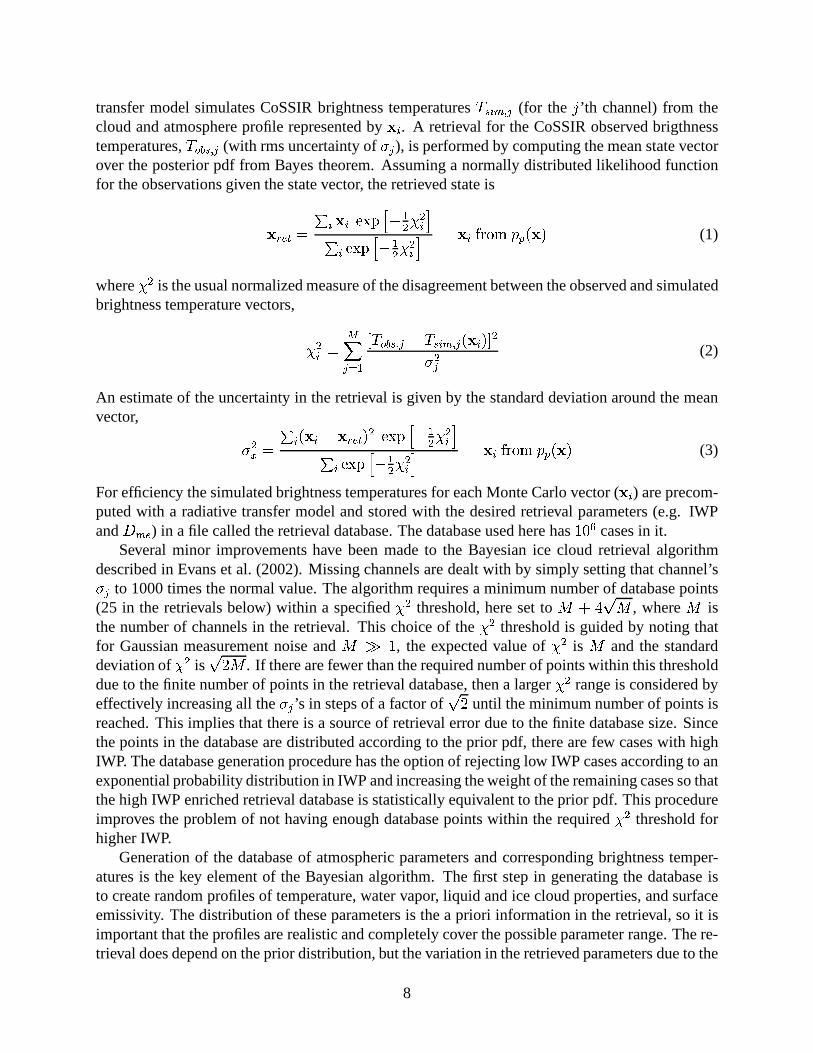
Besides using the CRS integrated backscattering to evaluate the CoSSIR retrievals, it can alsobe input to the Bayesian retrieval algorithm. In this case, there is no longer any validation, butit is still useful to see how the IWP andÃ Ä Å retrievals, and especially the error bars, behave. Inaddition to the integrated backscattering, the backscattering weighted cloud height is input to theBayesian algorithm. The calibration uncertainty (Æ ) in CRS integrated backscattering used for theretrieval is 1.0 dB, and theÆ for the weighted cloud height is taken to be 0.5 km (so as to notunnecessarily restrict the number of matching database cases). The retrieval results for July 28 arepresented here statistically in Fig. 7, which shows the median retrieved IWP andÃ Ä Å as a functionof integrated backscattering for CRS only, CoSSIR only, andCRS + CoSSIR retrievals. Overall,the retrievals for the three instrument configurations are fairly similar. In the thickest anvil regionsthe CRS only retrieved IWP is smaller than when CoSSIR data isincluded. The retrieved IWPerrors are smaller for CoSSIR only than for CRS only retrievals, and decrease further with thecombination. TheÃ Ä Å errors for the lowest integrated backscattering bin are actually larger forCoSSIR only than for CRS only retrievals because CoSSIR withthe noisy submillimeter channelslacks any sensitivity there. Except for the low reflectivityregions, theÃ Ä Å errors are much lowerfor the combination of CRS and CoSSIR data than for CRS alone.
5. CRS and CoSSIR profile retrievals
A new algorithm was devised to retrieve profiles of IWC andÃ Ä Å from the combination ofCRS radar reflectivity profiles and CoSSIR brightness temperatures. The major assumption of themethod is that the ice water content profile is related to the reflectivity profile byÇÈ É Ê ËÌÍ ÎÏÐ Ñ ÒÅ .However, the coefficientsÓ and Ô are retrieved for each column from the combined CRS andCoSSIR data in a Bayesian procedure.
14

-50 -45 -40 -35 -30 -25 -20 -15012345678
Med
ian
Diff
eren
ce(d
B)
July 3
Only 183,220183,220,380,640
-50 -45 -40 -35 -30 -25 -20 -15012345678
Med
ian
Diff
eren
ce(d
B)
July 7
Only 183,220183,220,380,640
-50 -45 -40 -35 -30 -25 -20 -15012345678
Med
ian
Diff
eren
ce(d
B)
July 28
Only 183,220183,220,380,640
-50 -45 -40 -35 -30 -25 -20 -15012345678
Med
ian
Diff
eren
ce(d
B)
July 29
Only 183,220183,220,640
-50 -45 -40 -35 -30 -25 -20 -15CRS Integrated Backscattering (dB /sr)
0
1
2
3
4
Med
ian
Nor
mal
ized
Diff
eren
ce
July 7July 3
Available channels
-50 -45 -40 -35 -30 -25 -20 -15CRS Integrated Backscattering (dB /sr)
0
1
2
3
4
Med
ian
Nor
mal
ized
Diff
eren
ce
July 29July 28
Available channels
Figure 6: The top four graphs show the median absolute difference between CoSSIR retrieved andCRS integrated backscattering as a function of CRS integrated backscattering (in 5 dB wide bins).The bottom two graphs show the median absolute normalized difference, where the normalizationis by the retrieved integrated backscattering error.
15
-50 -45 -40 -35 -30 -25 -20 -15CRS Integrated Backscattering (dB /sr)
100
300
100
300
1000
3000
10000M
edia
nIW
Por
IWP
erro
r(g
/m2 )
CRS+CoSSIRCoSSIR onlyCRS only
IWP errorIWP
July 28
-50 -45 -40 -35 -30 -25 -20 -15CRS Integrated Backscattering (dB /sr)
25
50
100
200
400
Med
ian
D meor
Dm
eer
ror
(m
)
CRS+CoSSIRCoSSIR onlyCRS only
Dme errorDme
July 28
Figure 7: Median retrieved IWP andÕ Ö × and errors for three combinations of CRS and CoSSIRdata plotted against integrated CRS backscattering (for 5 dB wide bins).
16
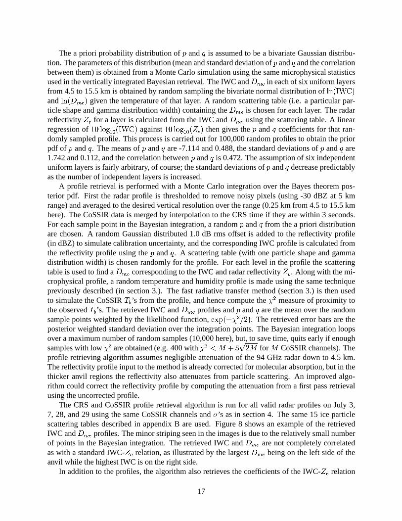
The a priori probability distribution ofØ andÙ is assumed to be a bivariate Gaussian distribu-tion. The parameters of this distribution (mean and standard deviation ofØ andÙ and the correlationbetween them) is obtained from a Monte Carlo simulation using the same microphysical statisticsused in the vertically integrated Bayesian retrieval. The IWC andÚ Û Ü in each of six uniform layersfrom 4.5 to 15.5 km is obtained by random sampling the bivariate normal distribution ofÝÞ ßàá â ãand ÝÞ ßÚ Û Ü ã given the temperature of that layer. A random scattering table (i.e. a particular par-ticle shape and gamma distribution width) containing theÚ Û Ü is chosen for each layer. The radarreflectivity äÜ for a layer is calculated from the IWC andÚ Û Ü using the scattering table. A linearregression ofåæ Ýçèéê ßàá â ã againståæ Ýçèéê ßäÜã then gives theØ andÙ coefficients for that ran-domly sampled profile. This process is carried out for 100,000 random profiles to obtain the priorpdf of Ø andÙ . The means ofØ andÙ are -7.114 and 0.488, the standard deviations ofØ andÙ are1.742 and 0.112, and the correlation betweenØ andÙ is 0.472. The assumption of six independentuniform layers is fairly arbitrary, of course; the standarddeviations ofØ andÙ decrease predictablyas the number of independent layers is increased.
A profile retrieval is performed with a Monte Carlo integration over the Bayes theorem pos-terior pdf. First the radar profile is thresholded to remove noisy pixels (using -30 dBZ at 5 kmrange) and averaged to the desired vertical resolution overthe range (0.25 km from 4.5 to 15.5 kmhere). The CoSSIR data is merged by interpolation to the CRS time if they are within 3 seconds.For each sample point in the Bayesian integration, a randomØ andÙ from the a priori distributionare chosen. A random Gaussian distributed 1.0 dB rms offset is added to the reflectivity profile(in dBZ) to simulate calibration uncertainty, and the corresponding IWC profile is calculated fromthe reflectivity profile using theØ and Ù . A scattering table (with one particle shape and gammadistribution width) is chosen randomly for the profile. For each level in the profile the scatteringtable is used to find aÚ Û Ü corresponding to the IWC and radar reflectivityäÜ. Along with the mi-crophysical profile, a random temperature and humidity profile is made using the same techniquepreviously described (in section 3.). The fast radiative transfer method (section 3.) is then usedto simulate the CoSSIRë ì ’s from the profile, and hence compute theíî measure of proximity tothe observedë ì’s. The retrieved IWC andÚ Û Ü profiles andØ andÙ are the mean over the randomsample points weighted by the likelihood function,ïðñ ßòíî óôã. The retrieved error bars are theposterior weighted standard deviation over the integration points. The Bayesian integration loopsover a maximum number of random samples (10,000 here), but, to save time, quits early if enoughsamples with lowíî are obtained (e.g. 400 withíî õ ö ÷ ø ù ôö for ö CoSSIR channels). Theprofile retrieving algorithm assumes negligible attenuation of the 94 GHz radar down to 4.5 km.The reflectivity profile input to the method is already corrected for molecular absorption, but in thethicker anvil regions the reflectivity also attenuates fromparticle scattering. An improved algo-rithm could correct the reflectivity profile by computing theattenuation from a first pass retrievalusing the uncorrected profile.
The CRS and CoSSIR profile retrieval algorithm is run for all valid radar profiles on July 3,7, 28, and 29 using the same CoSSIR channels andú ’s as in section 4. The same 15 ice particlescattering tables described in appendix B are used. Figure 8shows an example of the retrievedIWC andÚ Û Ü profiles. The minor striping seen in the images is due to the relatively small numberof points in the Bayesian integration. The retrieved IWC andÚ Û Ü are not completely correlatedas with a standard IWC-äÜ relation, as illustrated by the largestÚ Û Ü being on the left side of theanvil while the highest IWC is on the right side.
In addition to the profiles, the algorithm also retrieves thecoefficients of the IWC-äÜ relation
17

IWC
72200 72400 72600 72800 73000 73200
68
101214
Hei
ght (
km)
IWC error
72200 72400 72600 72800 73000 73200Time (UTC sec)
68
101214
Hei
ght (
km)
0.005 0.050 0.500 5.000
IWC (g/m^3)
Dme
72200 72400 72600 72800 73000 73200
68
101214
Hei
ght (
km)
Dme error
72200 72400 72600 72800 73000 73200Time (UTC sec)
68
101214
Hei
ght (
km)
30 63 134 283 600
Dme (µm)
Figure 8: Example IWC andû ü ý fields from the Bayesian CRS and CoSSIR profile retrievalalgorithm for July 29. 18
(þ andÿ) and their errors. Figure 9 plots the medianþ andÿ and errors as a function of the CRSintegrated backscattering. The mean and standard deviation of the retrieved coefficients is nearlythe same as the prior distribution when the integrated backscattering is below -35 dB. Presumablythis is due to the CoSSIR sensitivity being too low to affect the retrievals, which are effectivelyonly from the CRS in the thin anvil regions. At higher integrated backscattering values both theþandÿ coefficients increase away from the prior distribution meanand their uncertainties decrease.In the highest integrated backscattering bin, for example,the median coefficients areþ � �� ���andÿ � � ����, which give a 70% higher IWC for� � � mm�/m� than the a priori values (1.02vs. 0.60 g/m�).6. Conclusions
The Compact Scanning Submillimeter Imaging Radiometer (CoSSIR) first flew in July 2002during CRYSTAL-FACE. Scanning across track, CoSSIR measured brightness temperatures in 12channels with receivers at 183, 220, 380, 487, and 640 GHz. Although the submillimeter-wavechannels were noisier than anticipated, the CoSSIR data demonstrate the high sensitivity of thesubmillimeter channels to ice cloud particles as compared with the lower frequencies. A Bayesianalgorithm is used to retrieve ice water path (IWP) and medianvolume equivalent sphere diameter( �) from the available CoSSIR nadir brightness temperatures.Prior information used by thealgorithm is obtained from radiosondes and in situ cloud microphysical probes on the Citation air-craft flown in CRYSTAL-FACE. The retrievals are tested by retrieving vertically integrated 94 GHzradar backscattering from the CoSSIR data, which is then compared to Cloud Radar System (CRS)data. The integrated backscattering typically agrees to 1–2 dB for IWP from 1000 to 10,000 g/m�,while for lower IWP the typical agreement is 3–5 dB, which is within the Bayesian error bars.Retrievals of integrated backscattering using only the 183and 220 GHz CoSSIR channels havealmost as good agreement due to the high noise on the submillimeter channels.
An algorithm was developed to retrieve profiles of ice water content (IWC) and � from thecombination of CRS reflectivity profiles and CoSSIR brightness temperatures. A power law re-lation (��� � �� ��� � � ) is assumed between IWC and equivalent radar reflectivity (�), but theþ and ÿ coefficients are retrieved for each column. The IWC and � profiles andþ and ÿ areretrieved in a Bayesian integration that effectively matches the simulated and observed CoSSIRbrightness temperatures. The radiometer data adds additional information to the radar profile sothat the retrieved IWC and � are no longer completely dependent as they are with a traditionalIWC-� relation. The median retrievedþ and ÿ over all flights both increase from the a priorivalues for the highest IWP clouds. The results from the combined radar-radiometer profile algo-rithm illustrate how the coefficients for radar only ice cloud retrieval methods could be tuned forparticular cloud types using submillimeter radiometer data.
The CoSSIR only retrievals of IWP and � and the combined CoSSIR and CRS retrievals ofprofiles of IWC and � are available in the CRYSTAL-FACE archive athttp://espoarchive.nasa.gov/. During CRYSTAL-FACE the sensitivity of CoSSIR tolower IWP clouds was much poorer than anticipated due to the high noise of the submillimeter-wave channels. CoSSIR is currently being upgraded to improve the performance of the 380, 487,and 640 GHz receivers to noise equivalent temperatures of better than 1.0 K. The CoSSIR upgradewill also include the addition of a 874 GHz receiver for improved sensitivity to cirrus with smallerice particle size.
19

-50 -45 -40 -35 -30 -25 -20 -15CRS Integrated Backscattering (dB /sr)
-9.0
-8.5
-8.0
-7.5
-7.0
-6.5
-6.0
-5.5
-5.0
-4.5
-4.0M
edia
nre
trie
ved
pan
der
ror
IWC in g/m3
Ze in mm6/m
3IWC = 10
0.1pZe
q July 3, 7, 28, 29
-50 -45 -40 -35 -30 -25 -20 -15CRS Integrated Backscattering (dB /sr)
0.3
0.35
0.4
0.45
0.5
0.55
0.6
0.65
0.7
Med
ian
retr
ieve
dq
and
erro
r
Figure 9: Median retrieved� and � and median errors over all flights for the CRS + CoSSIRprofile retrieval algorithm. The� and� are coefficients in the power law ice water content - radarreflectivity relationship. The solid horizontal lines showthe a priori mean values of� and� , whilethe dotted lines show� one standard deviation.
20

AcknowledgementThe authors wish to thank Andy Heymsfield for microphysical advice andsharing a prepublication manuscript. Andy Heymsfield and Carl Schmitt provided the 2D-C/HVPSsize distributions and CPI imagery. Mike Poellot provided the Citation meteorological data andFSSP size distributions, Cyndi Twohy the CVI data, and LarryMiloshevich the radiosonde data,all from the CRYSTAL-FACE archive. KFE was supported in thiswork by NASA grant NAG5-11501. CoSSIR development was made possible through grantsfrom the NASA SBIR program,and funding from the NASA Goddard Space Flight Center Director’s Discretionary Fund and theNASA Radiation Sciences Program. The Cloud Radar System andLihua Li were supported by theRadiation Sciences Program at NASA headquarters.
21

A Particle size distribution analysis
The Bayesian ice cloud retrieval algorithm requires statistics on the relationship between tem-perature, IWC, and���. For CRYSTAL-FACE the best source of these microphysical statistics arethe optical cloud probes on the University of North Dakota Citation aircraft. The Citation flew at arange of lower altitudes compared to the WB-57 aircraft and thus is more representative of the mi-crophysics relevant for vertically integrated retrievals. Cloud probes that measure the particle sizedistribution are needed to calculate the��� for each sample. To cover the full range of ice particlesizes, data from three probes are used: the PMS forward scattering spectrometer probe (FSSP),the PMS 2D-C imaging probe, and the SPEC, Inc. high volume particle spectrometer (HVPS).The 2D-C probe has 33�m resolution, sizes up to 1000�m , and samples about 0.007 m�/s. TheHVPS probe has 200�m resolution, sizes up to 6000�m , and samples about 1 m�/s. The FSSPmeasures size distributions from about 4 to 62�m and is the only source available for the smallerice crystals, though the concentrations tend to be overestimated due to large particle breakup andthe assumption of particle sphericity.
The composite 2D-C/HVPS size distributions and the FSSP size distributions available fromthe CRYSTAL-FACE data archive are analyzed in a technique similar to that in Heymsfield et al.(2004). A particle mass - maximum diameter relation of the form ! "#� $ % is assumed, and thecoefficients"# and" & are adjusted to match the IWC measured by the counterflow virtual impactor(CVI) (Twohy et al., 1997). The first step is to average and merge the archived temperature,CVI IWC, and FSSP data to the 5 second samples of the 2D-C/HVPSsize distributions for allCRYSTAL-FACE Citation flights. The particle mass for each bin in a measured size distributionmay be obtained from the central maximum diameter using the mass-diameter relation for a given"# and" &. The IWC is then simply the sum over the bins of the particle mass times the numberconcentration. The procedure for determining the best fitting coefficients has two steps. The first isto try a fixed" & and adjust"# so that the median (over all samples) of the ratio' of the computedIWC to the CVI IWC is unity. The coefficient" & is then determined by adjusting it to minimizethe ratio'() *'+), where'+) and'() are the 25th and 75th percentiles, respectively, of the ratio' . The first step assures an unbiased fit, while the second step minimizes the dispersion of theoptical probe IWC around the CVI IWC. We expect that using percentiles is more robust to errorssuch as the CVI hysteresis. This procedure is carried out only for samples above the nominalCVI sensitivity of 0.01 g/m� and for temperatures below -5 C. The best fitting mass-diametercoefficients from this procedure are"#=0.00423 and" &=2.12 in cgs units. Figure 10 shows ascatterplot of the resulting optical probe and CVI IWC. These coefficients give a somewhat lowerIWC than those in Heymsfield et al. (2004), which are"#=0.00513 and" &=2.10.
The mass-diameter relation with the tuned coefficients is used to calculate moments of the massequivalent sphere diameter,��, from the FSSP plus the 2D-C/HVPS size distributions (only sam-ples with nonzero 2D-C/HVPS IWC are used). The IWC and��� are derived by fitting gammadistributions (, -�� . / � 0� 123 45 -6 7 8 9:;.� �*���< with 6 ! =) to the third and fourth momentsof �� (see, e.g. Evans et al., 1998). Processing all 14 Citation flights results in temperature, IWC,and��� for 13891 samples with IWC above 0.001 g/m�. The microphysical probability distri-bution in the Bayesian retrieval algorithm assumes a Gaussian distribution of temperature. Sincethe Citation sampling of temperature is experiment dependent and has nothing to do with micro-physics, the microphysical samples are randomly selected to make the temperature distributionmore Gaussian. This process outputs 5000 samples approximately matching a target distribution
22

0.003 0.01 0.03 0.1 0.3 1 3CVI IWC (g/m
3)
0.003
0.01
0.03
0.1
0.3
1
3
Opt
ical
prob
eIW
C(g
/m3 )
IWC from 2DC+HVPS+FSSP probes and CVI
.
.
................ ..
..
..
.
.
.
..
.
.
. ...
..
....
.
..
.
.
..
.
.
.
.
.
.
.
.
.
. ..
.
.
. .
.....
............
. ..... .........
..
.
.
..
..
. .....
.. .
... .
.
.
.
.
.
.
.....
.
.
.
. ..
.
.
....
.
.
..
..
..
. .
..
.
.....
..
.
.
..
..
.
.
..
.
.
.
...
...
...
.
.
.
.
.
.
.
.
.
.
...
.
.
.
.
.
.
.
.
.
.
.
. ..
..
.
.
.
.
.
.
.
. .....
. ...
..
.
.
.
.
.
. .. ..
....
..
.
.
.
.
...
.
... ..
..
.
.
. . .
.
..
. ...
.
.
..
..
.
. ...
..
. .
. ..
.....
...
.
.
. ...
.. . ...
...
. . ...
..
..
..
.
.. . .
..
.. .
.
..
...
.
.
..
... .
..
.
.
.
. ..
.
.
.
.
...
.
.
.
. .............
...
....
.
.
.
.
.
.
..
. .
.
.......
.
.
...
.
...
..
.
.
. .. .
.
.
...
.
..
.
.
..
..
.
..
.
.
.
...
..
.
..
.
...
.
. ..
.
.
..
.
.
.
.
.
.
.
.
.
.
.
..
.
.. ..
. ..
...
.
..
.....
.
.................
.
.
........
.
.
.
...
...
.
.
....
...
...
.
..
.
..
.
.
...
..
..........
.......
. .
...... .
.
.
.
.
.....
.
.
..
.
.
..
...
....
...
................
..
..
..
.
.
...
.
.
..
.
..
..
.
. .
..
.. .
.
.
.
.
.
. .
..............
..........................
.........
. ......
......
................
.......
.......
...
.....
.
....
.
..
.....
..
..
. . .....
.....................
..
.
. .. .
... .. . .
...... . . ....
..
.. .
..
..
..
.
.
.
.
.
.
..
.
..
.
.
.
.
.
..
.
.
.
.
..... .
..... ......
....
....
..
.
..
...
.
.
....
..
.....
...
.
................
.
..
.
.
..
.
.
..
.
.....
... .
. . .......
...
..
...
. ..
..
..
..
.......
.
.
..
..
.
. .
. .
.
. ..
........... . .
....
.........
... ....
.... ..
.. .........
.. .... .. ..
.. .
..... ........... .. ..... .
. .. ..
... ..... .
... ...
.... .. .. ..
.. .. .. .. .... .
...
... .
..
..
..
...
.
.
.
.
.
.
.
.
.
.
. . . ...
.... ..
.. .....
..
.. ..
... ... ..... .
.....
.
....
.
...
..
...
....
. ... ....
..
.... . .
.
.. ....... ............... . ...
..... .......
..
.
.
. .
..
..
...
.
.
..
.
..
. .. ..
..
.
. ..
....
.
.
.
..
..
....
.
..
. .
.
..
.
.
.
.
. .
..
.
.
..
.
. .
..
.
.
.
.
.
. ..
..
.
.
.
....
.
.. .
..
.
. .
..
.. . .
.
. .....
.
..
.
.
..
.....
.
.
. .. ...... .
.. . ....
..
...
.
.
.
.
.
.
..
..
.
.
.
.
.. .
......... ... .
.
. ...
...
.
.
.
..
. .
.
.
..
..
. .. .. .
. . . .... . .
.
. ... .
...
..
.
.
.
.
.
..
. .
.......
.. .. .
....
.
.. ..
.
..
..
...
.
.
.
.
..
...
.
....
. . ..... ..
. ..... .. ....
..
..
.....
.
. .
......
..
..
..
..
.. ..
. ..
.
... ...
.... ...
..
...
......
.
.......
.
.
.
. .
. ..
.
.
.
.
..
.
...
.
.
.
. . ... .. .
..
....
.
.
..
......
....
..... . .....
.. .....
.
..
...... .
.
.. ... .
..
.. ....
... .
. . . .. . ..
. .. ..
... .
. .............
. ..
...... .. . ...........
. . .
.... ...
...
. ..................... ...
.... ...
..
..
..
........
.........
.....
.... ...
.......
.....
..... ....
. .
... .........
...
.....
... ... ... ..
...... .. .. . .... .
..
..
......
. .... ..
. ..
.. .. .. ..
.... .....
..
. .........
....
..
...
.
.
..
.
.
.
.
..
. .
.
.
.
..
..
..
.
.
..
..
... .
..
.. .. .
.
.
.
.
..... .
. .. .
...
. .
.
...
..
....
..
. .... ..
. ...... ..
.
.
...
.
.
... .
.. .
........ ..
..
.
.
.
. .
.
.
.. .
. ....
...
. .
...
.
.
.
. ...
..
..
...
. .
.. .
.
.. .
.
.
.
.
.. .
. .
.
.
.
.
. . .
...
..
..
..
.
..
. ...
.
. .. ...
.. .
.
.
..
..
.
.
. ..
.
.
. .. .....
.
.
.
.
.
.
.
.
..
.
.
.
.
.
..
.... .
.....
...
.
.
.
.
.
.
..
.
..
..
... ...
.
.
..
.
.
..
.
. .
.
.
.
.
.
.
..
. .. .
.........
... .
..
.
..
.
. . .
..
. ..
.
.
.
.
.
.
.
.
. ....
. . ...
......
.
........
....
..
..
.......
...
.....
.
......
... .....
..
.. .
.
.
.
. . .
. .
...
..
..
. ..
. .
.
.. .
..
.
..
.
...
..
..
...
...
.
..
. ... ...
. .....
.
.
....
..
....... ..
..
.
..... ....
.
. .. ...
.
..... ..
.
..
.....
..
... ....
.......
. ..
.. .... .. ..
. . ....... . ..
.. ..
.
.. .
.
.
.
.
..
.
.. .
.
.
.
.
.
. .
.
.
.
. ...
.. ...
....
..
..
.
.
.
.. .
......
.
.
..
...
.
.
.
.
.
..
..
.
. .....
....
.
.
..
..
.
.. ...
. ..
.. .
..
.. ...
. .. ...... ... .
. ...
..
..
..
.....
......
...
..
.
..
....
...
... .....
.
.
...
.
..
.
.....
...
.
...... ......
.
..........
.... .
.
.
... .
.
.
.
. ... ...
.... ...
... ...
..
.
.... .
...
..
...
. .. .
. ..
...
....
..
....
. .... ..
.
..
.
...
......
. .....
...
..
..
..
.
..
.
..
.
...
...
.
.
.
.
.
.. ..
... .
.
.... .
.....
. . .. ..
..... ...
.. ......
....
... ..
. .
.
.. ..
.
...
....
.
.. .
.
.....
. .... . . ...
.. .
. . .....
..
....
...
..
..
...
. ...
.
...
.
.
.
.
. .. ....
.....
.
....
.. .. .
.
... ....
.
....
. ...
......
. .......
....
. .......
...
.
. ..
......
. ....... ...
.
.
.........
..
..
..
...
. ..
...
. ..
.. . .. ..
. .....
........
. ...
.... .
. ... ..
.....
......... ..
....
...... .
. ....
..
. ..
.. .....
..
.....
..
.
.
.
...
.
.. ..
...
.. .
..
...
.
.
.
.
..
. .
.
.
. .
....
.
..
..
... . ...
..
.
..
.... .. ..
..
. ..
... .
...
...
.
... .
. ..
...
.
. ....
...... ...... .....
..
...... .....
.....
....
.. ..
.. .
...
....
..
...
...
.....
..
.
.
. . ....
.......
..
..
.... .... .
.
.
...
. . .
.....
..
.. . .
.
....
. ....
....
..
.
.....
.
..
.
.
. .
.
.
.
.
.
. . .... . . .. . .. ..
.
.
...
.
..
. ..
. .
.. ....
..
. .. . ... ...
. ....... .......
.........
.. ..
.
.
.
.
..
...
.
.
.. .
......
..
... .
.
.... ....
.
. .
.
.
..
. .
.
.
.
..
.
.
.
.
.. .
.
.
..
.
...
..
.
..
.. .
.
.
.
......
. ............... ..
.
.
....
.
..
. ..
. . .
....
.
...
.. .... .
..
.
..
.
..
.
. ..
..
..
.. ..
. .. ...
.. ...
. . ... . ... ..
..... .....
. ..... ...
.. ..... ....
. .
.
..
.. ... ... .
.............
.. ..... .
...
.
....
. ...
.
.. . ..
..
.....
. ....
.. . ....
..
.
.
.
. .... . .........
. . .
.... .....
..
. .
. . ... .............. ..
.
.
.
. ..
. ....... .
... ........
............. . . ..
.
..
. . ..............
...
.
.
...
. ...
.
.
.
.
.
.
.
.
..
..
..
. ... . ........
..
.
..
. ...
..
.
...
.
.
.
...
.
..
.
.
..
.
.
.
..
.
. ..
. ..
.
.
..
..
.
..
.. .
...
..
..
.
.
.
....
.. .
.
..
.
. .
...
.
..
.
..
...
.
....
.
.
.
.
.
.....
..
..
..
...
..... ..
..
.
.
.
.
.
.
.
.
..
....
.. ....... ... ......
.
..
..
. ......
.. ....
.. ....
....
....... .. ..
. ..
. ...
.
..
. .............
........
.
.
.
.
..
.
...
......... .......
.......
...........
....
.
....
...
........
..
...
.
.
..
...
..
.
.
.
...
.........
......
... .
.. ... .
...
..........................
....
.......
..
...
... .
. ... .........
....
........... ................
.....
..
.
..
.....
.
. .....
..
. .........
.
.
.
.
.....
...
.
......
....
..
...
.. .. .
. .................
...
......
...... ..
. ......
.. ...
.
.
.
.
..
.
.
.
..
..
. .
.
..
.
.
.
..
.
.
.
...
. .....
. ... ..
.........
. ......... ..
.
..............
.
.
...
...... ..
..........
.
... .....
. ...... .......
..
...
.
.
.. ..
...
. ... .
.. . .
... .
..
. .............
.............
. .. ... .
.
..
. ............ ... ....
.......... ...
. ........... ..
....... ....
....
.
. ..
.
...
.
....
.
.
..
..
..
.
. ..
........
.
.. .. .....
. ...
.........................
... .... .. ... ... .............
..
......
... .
..... .
....
...
..
.
.
.
..
.
.
....
..
.
. ................
.. ........... ....... .... ..
...
..
....
. .....
........ ...........
....
.. .......................... .. .......
.........
.
.. ..
. .
.
.
..
.
.
.
.
.
.
. ..
..
....
.
...
.
.
. .
..
..
.
.
...
.
.
.
.
.
....
.
..
..
.. ..
.
..
...
...
.
. . . ........ ..
. . .. . . ..........................
....
...
..
.
..
...
. . . ... .
.
.
.
.
. .
.
. .
. .. .. . ..
.....
.. ..
. ........
.....
..
.
.
.
. .. .
.. .
..... .
.........
....
..
.
.
. ..
...
.
.
.
.
..
.
. ...
. ...
.
...
..
..
..
.
.... .
..
.
.
....
.
.
.
.
.
.
...
.
...
..
.
.
.
..
.. . .
.
.
.
. ...
.. .. .
.....
. .
..
.
.
.
.
.
..
.
.
.
.
.
...
.
..
.
.
.
..
. .
. ...
.
.
.
..
.
.
.
.
.
.
.
.
.
.
. ..
.... .
...
.......
..
. ..
...
..
.
.
.
.
.
.
..
..
.
..
.
.
..
. ..
...
...
.
.
..
.
.
..
.
.
. ....................................... ...
..... .........
................... ......................................... ............... .............
. ......................... ..... .......... ........
.....
.. ......
... .................... .
. ........
.. ........... .... .. .....
...
.......
.. ..
...
........ ..... ........
.. ....
. .......
....... .. ... ..
.. ...
...
.
. .
...
...
.... ... ......
.
.
.
..
... .
.
.
.
.
.
..
... . .
. ......
. ... . ...
. .. ... .
............
. ....... . ..
. ...........
..
.
.
.
.
..
.
.
..
..
. .
.
..
.
.
.
.
.
.
.
.
..
.
. .
.
.
.
.
.
.
.
.
.
. .
.
.
.
..
. . ...
..
..
. .
.........
...
.
.
..
..
.
.
. ..........
.
.
.
.
.
.
.
.
.
.
... .
.
..
... .... ..
............
..
..
. ......
..... .....
.
.
.. ....
...
..
.
..
.
..
.
.
.
.
.
...
. ..
.
..
.
...
.
.
.
. ..
..
. .. . .....
..
.
.
.
....
..
.
.
.
... .....
..
......
.
.. ..
.
.
..
.. ...
..
.
.
.
.
.
.
.
.
.
.
..
. .
.
. .
..
..
.
.
..
.
. .
..
. ...
.
. . ..... .. ..
. .
...
...... ....
.
.
.
..
..
..
.
.
..
....
.
...
. .....
......
.....
...
... ......
...
...
.....
..
....
.
.
.
..... .
.
....
..
.
..
.
. .. ..
.
.
.
.
..
.. ..
..
.... .. .
.....
. ........ ....
. . ...
...
.
.
..
.
. ..
.
.
.
.
.
.
.
.
. .
. ..
.
.
.
.
. ... ..
....
. ........ .......
..... ....
. ....
...
..
.. .
..
.
.
..
.
..
.
.
... ...
. ...
...
...
.
..
..............
.... ..
..... .
........ ...
... ...... ............. .
.. ..
.
...
...
.
..
.
. ...
.
.
... .
... . .. .
. .........
. ....... .. .. ...
. ...........
. . ....
..........
..
.
...
.
.
.
..... .
.. ... .....
.
.
.
. .
.
.. .
.. .
.. ...
..
....
. ...... .... . . .. . ...
.
.
.
... ..... ....
.
..
..
.
.. ..
..
.. ....... .
. ..
.. ..
..
... ..
. ..
... .
..
. ....
...
. .
..
..
.
.
.
.
...
..
.
.... ..
..
.
.
.
. ...
.
.
.
.
.
. .
.
...
.. .......
.
.. .
.
. ....
... ....
....
..
.
..
.. .
.
.
... ..
.... ...
. .... ........... .
.. .... ......... .
.
.
.
.
..
.
.
.
.
.. .
. ...
.. .. .. .... ... . ...
... . . .. ..
.
..
.. ...
.
.
.
..
..
..
.
.
.
.
.
. .. .
..
. ...
..
...
.....
.
..
... . ..
.
. .
... . .
. .
..
..
... ..
...
... ..
..
.
.
. .
...
...
.
.
.
...
...
.
..
..
.
...
..
...
.....
.
...
....
.....
.. .
. ........ ....
..
..
.
.
.
.
.
.
.
.
.
.
.
.
.
..
.
. .
.
.
.
.. .
.
.
.
.
.
..
.
.
.
..
.. .
.
.
..
..
.
.. ..
. . ....
.. .....
..
..
.
....
.
.
. ..
. .
.
.
.
..
..
. . ... .
...
....
..
.
.
.
.
.
..
..
..
.. ..
.
..
.
.
.
.
. . . ...
. .... . .. .....
. .. . .......
..
..
..
.
. .....
. .... ...
. ..
........
....
... ...... .. .
. ..... . .... ..
.
. ...... .... . ........
. .....
. ...
..
.
...
.
..
..
.
. .
. . .. ... . .. ....
........ ....
.. .
..
.
.
.
.
.
.
. .
. .
..
..
..
..
...
.....
........... .. .
.......
. ..
.
.
.
.
.
...
.
. .
.
..
..
.
.
. .
.
.
.
...
. .. . .
..
.. .... ....
........ ..
. . ................
...
.
..
.
. .. ...
..
...
.
.. .. .
...
. . ....
......... ...
..
. . . .....
......
. .. ..
.. ..
. .... ..
...
...
.. . .
.
.
.
. .. .
...
. ..
...
.
.
..
.
..
.. .
. .
.
..
.
.
.
..
.
. .. .
. ...
. .......
.......
...
. .. ..........
.
..... ....
.....
. .. .
... .......
. ..
.
..
. .
. ..
.. .
.
.. .
.. .
.
. .
.
.
.. .
.. ....... ... . ..
..
..
. .
. ..
. ...... .
...
..
.
..
..
.. .
.....
..
.
.
.. . . .
.
. .....
. ... .
.... ..
...
.
.
.
.
.
.
.
..
.
.
.
.
. .
..
...
.
.
.
.
. .
.
...
..
. .... .
. .. ... ........
...
..
.
. ...
.
.
.
. .
..
.
.
. ...
...
..
..
.
.
.
..
.
..
.
. . .. .
. ... .. .
.... ...
. .. .
...... .
...
. ..
..
.....
...
.
..
.... ..
.
.
. .. .
.. ...
..
... ... ...
..
.
....
.
..
. .
. ..
.. .
. .
. ...
.................
.. .. ....
.....
.........
.. ..
.
..
..
.
.
.
. .
.
..
.
.
.
...
. .
.
..
...
..
. .
.
.
.
.
.
.
..
.
.
.
.
..
.
.. .
.
.
...
..
.
.
.
. .
. .
...
........
..
...
...
.
.
.
.
.
.
. ..
.
.
. .
...
.
.
. ..
. ......
. .. ...
.
. .
...
.
..
...
..
..
.
.
.
...
.
.
.
.
.
. .
.....
..
.. .
.
. .
..
.
.
.....
...
..
..
..
.
.. .
.
.
.
..
...
. ..... .
....
....
.
..
.
.
.. ..
..... ..
.
.
.... ...... .
. .. .
...
..
.
. .. ..
...
.
... .
... ..
.
..
..
..
.
..
.
.
. .. ..
..
.
.
..
.
..
...
.
.
. .
...
...
. ...
....
..
... ..
.
...
...
.
.
..
.
...
... . . . . ...
.... .... .
...
.
..
...
. ........... ....
..
.
.
...
.
.
.
. ....
.
...
.....
.
.
.
...
..
....
..
.....
.....
...
........
.
. ..
...
.
.. ....
... .
....
. ..
.
.
.......
.
..
.
. ..
... .
..
.
.
.
. .
.
.. .
... ..
.. .
..
...
.
. ..
.
.
.
.
.. .
. ..
...
.
..
. ...
. ......
....
...
..
..
..
. .
...
..
....
. .
..
.
.
..
...
.......
.
. . ......
. ..........
.......
...
..
.
.
.
..
.
. .
....
..
.
.
.
..
.
.
...
. .
.. ...
.
.
.
.
.
..
................
..... .
..
..
...
..
..
..
. ..
.
..
.
...
..
.
.
.
.. .........
..
.
.
.
..
..
..
. .
...
..
.
.. .
...
.
.
.. .
.
.. ..
..
.
.
..
..
.
...
......
...
... .
.
.
. . ..
..
..
.
..
. ...
.. .
...
. .
... .
..
.
.
.
..
.
...
..
..
. ..
..
..
.
..
.
..
...
..
...
.
..
.. .
.. .....
....
.
....
..
.. .
...
.
...
.
.
..
...
. . .. ... ..
. .....
..
.. ....
.
..
...
.
.
..
.
.
......
.
.
.
.
.
..
...
....
..
.
.....
..
.. . ..
.
... ..
.
.
.
..
.
.
.
.. ...
.
.
.
.
..
.
.
.
.
.. .
..
..
.
..
.
...
..
.
.
.
.
.
.
..
.
..
.
..
.
...
....
.
.
.
.. ...
.. .
.
.
..
...
.
. .
.
.
.....
.
.. .....
.. .. .
.
.
.
.
.
.
.
..
.
.
.
..
.
.
.
.
..
.
.
..
........
..
.
.
..
...
.
..
.
..
...
.
.
.
.
..
..
.
.
.
..
..
.
.
.
. ..
...
.
. .
.. .
.
.
.
..
.
. ..
..
..
.
. .
.
..
.
.
..
....
.
.
.
.
.
.
.
.
.
.
.. .
.
. ..
..
..
..
.
.
..
. .
. .
..
. ..
.
.
. .
.
.
...
....
...
..
.
.
..
.
.
.
...
.
.
.
.
. ..
..
.
. ....
.
...
.
.
.
.
.
. ..
.
.
.
.
...
..
.
..
..
.
.
...
.
....
.
.
. ..
.
..
. .
.
...
.
..
..
..
. ..
..
.
. .
...
..
..
..
.. .
.
...
.
.
...
.
..
.. .
.
..
.
.
.
.
.
.
.
..
.
..
.
. ......
.
.
. .....
.
.
.
.
. .
.
..
..
. .
.
.
...
.
. .
.....
...
..
.. ..
..
.
..
..
.
..
...
.
..
.
..
.
.
.
.
..
.
.
...
..
.
... ... .
...
. ..
.
....
...
.
. .
.. .
.
..
.
. ..
.. ..
.
.
..
..
..
....
....
........ ..
...
..
. .
. ...
. ...
..
...
. .
..
.
.
..
.
.
.
.
.
.
.
.
..
.
.
.
..
.
. .
.
..
..
..
..
.... . ..
..
.
..
..
..
.
.
.
...
.
..
.
.
. .
.
..
.
..
.
...
.. ..
.
.
.
. .
..
..
..
..
.
.
..
..
. .
..
.
...
...
..
...
.......
....
..
...
... ..
.. ..
.. .
.. ... .
.. ..
.
.. ....
..
.. .....
......
...
. ..
..
.
.. .
..
..
....
.
..
.
.
. ....
..
..
.
. ..
.. .......
.. ...
...
.
..
..
..
..
. .... . ... ... ..
....
...... ....
. .. .. .......
...
. .
.......
...
...
. . . ..
. ....
... ...
. ....
..
.. ....
...... .
. . ... .. . ......
.. ....
.. ...
....
............. ..
.. .
. ...
. . .......
.....
....
..
....
.... . .... ..
. .. ...........
...
...... ..
..
.
.. .
..
...
........
... .
.. ...
..
. ..
..
.
..
.
.
.
..
.. .
..
.
.
.
.
.
.
.
.
.
.
..
. ..
. ....
..
........
..............
..
.
..
.
..
.
.
.
....
.
..
..
.
.
.
..
.
.
..
..
... .
..
.
. ........
.... .... ............... .
....
..............
....
.....................
.....
........................
. .....
....... ...............
..... ....
.
.... ...........
.... ..
.................
... ....
........................... .....................
.....
...........................
. ... ...................
...
.......
... ......................
............. ....
.... .. .... .... .
. ....... ..
....... ...
..... ........ ...
...... .
....
..... ..............
... ...... .
.... .... ................
...... . ............... ...... . .. ... .. ...........
...... .. . .... . ....
............... ..
.
. .. ...
.... .... ..... .
..
..
.
.
.
.
..
.
..
.
..
.
.
. .
.
..
.
..
... .
.
... .
... .
.
..
.....
...
..
.
.
.
.
..
.
.
.
.
.
.
.
.
.
.
.
..
...
...
.
.
......
.
...
.
. ...
.
.
.
.
.
.
...
. .
.
..
..
..
.
.
.
.
.
.
.
. .
.
..
.
.
.
.
. ..
..
.
.
.
.
.
.
.
.
..
.
.
.
. .
.
. .
.
.
..
.
. ....
..
.
.......
. .....
..
... ...
...
.... .
..
.. ..
..... .
.
..
.
.
...
..
..
.
.
..
.
..
..
... .
..........
... ..............................
.
...
.
..
.
.
.
..
...
.
.......
.
.
......
.
.........
.
.
...
.......
..
........
........
..............
..
....
.
. ... ..
..
. ...
...... .
.. . .. .... .
..
. .. ..... .. ..
..
.......
.....
......
..
......
.
..............
.
. .......................
..
.
..
.
.
.
.
.
.
..
.
.
. ...
...
.
.
..
.
..
...
...
..
...
.
.
.
...
.
.
.
......
.. ......
....
.....
. .......
....
...
. ....
.....
.
....
..
.
.
. ...
.
.
. ..... .
..
.. .
.............................................................
.. .
.
.
.
...
.
.
.
......
...
......
...
..
.
.
.
.
.. .
.
.
. ... .
.
.
.
..
...
....
..
......
.
. . . . .. .. ..
. .
.
. ........ ...
...................
.............
........
.. .................
........................ ...
...
.....
...
.
.
..
..
.
..
....
....
.. .......
..
. ..
....
.........
.....
........
.
...
.............
.
........ ......
..
.
.........
................
..
..... ....
....
....... ..............
. ...
.
. ....
.
....
.......
...
.
...
.
.
....
.
....
. ......
.........
.............
...
......
........
..
....
...
.
.
.
.
.
..
..
.... ..
..
............. ...
..........
. .... .........
.. ...
.
.. . .
.
All 14 Citation CRYSTAL-FACE flights
g0=0.00423 g1=2.12m = g0 D
g1 (cgs units)
Figure 10: Comparison of the IWC calculated from the opticalprobe size distributions using thebest fitting mass-diameter relation with the counterflow virtual impactor (CVI) IWC.
23

with a mean of 235 K and standard deviation of 15 K. Figure 11 shows the relationships betweentemperature, IWC, and>?@ for these 5000 samples. Table 4 lists the statistics of temperature,AB CDEFG
, andAB C>?@ G which are input to the Bayesian retrieval algorithm.
B Particle shape modeling
The ice particle shapes observed during CRYSTAL-FACE were most often complex irregularparticles. Figure 12 shows a typical cloud particle imager (CPI) picture of the particles in a densepart of an anvil. The complex particles often appear to be aggregates of hexagonal plates. Inaddition there are small, quasi-spherical particles whichappear to be frozen droplets. The CoSSIRand CRS retrieval algorithms require us to model the millimeter-wave and submillimeter-wavescattering properties of distributions of these complex particles. The highest CoSSIR frequency issensitive to features down to about 50Hm , so it is the larger scale particle structure about whichwe need to be concerned.
The CPI images inspired us to model the complex “junk ice” particles as random aggregates ofhexagonal plates and columns. The algorithm for generatingthese particles starts with a specifiednumber of randomly oriented hexagonal plate and column monomers of a fixed size. An aggregateparticle is represented by the position and orientations ofthe monomers of which it is made. Theparticles are projected onto Z-buffer images for 46 orientations covering all viewing directions at aspacing of about 30I. A Z-buffer gives the depth (positive or negative) of the particle at each pixelwhen viewed from a particular direction. Two particles are chosen at random to aggregate, andone of the 46 orientations is also chosen at random for each particle. The two particle Z-buffers forthese orientations and a random sideways offset between thetwo particles are used to determinewhen the particles touch (a certain amount of overlap may be specified). The two particles arethen combined by rotating the first particle to the second particle’s coordinates to make a newaggregate particle. The Z-buffer images are made for the newaggregated particle. This process ofaggregating (potentially already aggregated) particles proceeds until there is only one particle left,which contains all of the original monomers.
Three sets of random hexagonal aggregate particles are created. The first set of 20 sizes ofhexagonal plate aggregates has monomers with a maximum diameter of 230Hm and thickness of25Hm . The second set of 20 sizes of plate aggregates has thicker plates with a maximum diameterof 210 Hm and thickness of 30Hm . The last set has plates (diameter of 230Hm and thicknessof 25 Hm ) for 75% of the monomers and hexagonal columns (diameter of115 Hm and lengthof 300Hm ) for 25% of the monomers (18 particle sizes). Figure 13 shows one example particleimage from each of the three sets. The maximum number of monomers modeled is determined by
Table 4: Microphysical Input Statistics
Temperature (K)AB CDEF JKLM N OG AB C>?@ JHM OG
mean 236.5 -2.65 5.09std. dev. 12.2 1.82 0.766correlation PQ RST U V0.402 PQ RWXY V0.605 PST U RWXY V0.586
24

210 220 230 240 250 260 270Temperature (K)
25
50
100
200
500
1000
2000
Dm
e(
m)
CRYSTAL Microphysics
..........
..
.
.
.
..
..
..
.
.
....
.
.
.
.
...
...
.....
..
.
..
.
.
..
...
..
.
.
.
.
.
..
.
.
.
..
..
....
.
..
.
...
.
..
..
..
.
.
.
.
.....
..
........
.
....
.
...
.
.....
....
.........
....
.
..
....
.
..........
..
.....
...
..
..
..
...
.
.
.
...
.
.
...
.
.
....
.
.
....................
..
.
...
.
..
.
..........
.
.
..
..
.....
....
.
..
.
......
.
.
.
.
.
.......
.........
....
.
.
.
..
..
.
.
.
.
.
.
.
....
.
..
.....
.
.
..
..
.
..
.
.
..
...
...
..
.
....
.
...
..
..
.
....
...
...
..
.
.
..
.
.
.
...
.
.
.
.
..
.
.
.
.
.
.
..
.
.
..
.
.
..
..
.
...
.
.
.
.
..
.
.
.
.
.
.
..
.
.
.
..
.
.
.
..
..
.
.
.
.
..
.
.
....
.
.
...
.
..
.
.....
.
.
.
...
..
.
.
.
.
.
.
...
..
.
.
.
..
.
.......
.
.
.
............
.
..
..
....
..
.
.....
..
..
.
.
..
.
.
.
.
.
..
.
..
.
.
....
.
..
...
.
....
.
.
.
.
.
.
.
.....
.
..
.
.
.
....
..
.
..
.....
.
.
..
.
..
.
.
.
.......
.
.
.
.
.
.
.
.
..
....
.
.....
.
.
...
..
.....
..
.
..
.
...
.
.
.
.
....
.
.
.
.
.
.
..
.
.
.
.
....
..
.
.
.
.
.
...
.
....
.
.
.
.
..
..
.
.
.
.
...
.
.
....
.
.
.
..
.
.
..
.
.....
.
.
.
....
..
....
.
.
.
.
.........
.
.
.....
.
.
.
.
..
.
.
..
.
..
.
.....
..
.
.
.
.
...
...
...
..
..
.......
.
..
.
.
.
.
.
.
...
..
.
.
..
...
......
.
..
.
.......
.....
..
.
.
.
.
.
.
.
..
..
..
..
..
.
.
..
.
.
..
....
.
....
.
..
....
.
.
.
.
.
.
..
.
.
...
.
.
.
.
.
...
.
.
.
..
..
.
.
..
.
...
.
....
.
.
.
..
.
.
.
.
.
..
.
.
.
.
.
.
.
..
..
...
.
.
.
.
.
.
.
...
.
..
.
.
.
.
.
...
.
.
.
..
.
.
.
.
.
.
.
.
..
.
..
.
.
.
.
.
.
.
.
.
.
.
.
.
.
.
.
.
.
..
.
.
.
.
.
.
.
.
.
.
.
.
.
..
.
.
..
.
.
.
.
.
..
.
..
..
.
....
.
...
..
...
..
.
.
.
..
.
.
..
.
.
.
.
.
.
.
.
..
.
.
..
.
.
..
.....
.
.
..
.
.
.
..
..
.
.
...
.
.
..
.
.
.
.
.
...
.
.
.
.
..
.
..
.
..
.
.
.
.
.
.
.
....
.
.
.
.
.
.
.
.
..
.
.
...
.
..
....
.
.
.
.
.
.
.
.
.
..
.
.
.
..
..
.
..
.
..
.
.
.
.
.
.
.....
.
.
.
.
.
.
.
.
.
.
....
...
.
.
..
.
..
...
..
.
.
.
.......
..
....
..
.
.
.
.
.
.
.
..
.
.
.
..
.
..
.
....
.
.
..
..
.
.
.
..
.
.
.
....
..
.
.
.
..
.
.
.
.
.
.
.
.
.
.
.
.
..
..
.
..
.
....
.
.
..
.
.
.
.
..
.
.
.
..
.
.
.
.
.
.....
.
......
.
.
.
...
.
.
.
.
...
.
.
..
.
.
.
.....
.
.
...
.
.
.
.
..
..
..
.
.
.
.
.
..
.
..
..
..
.
....
.....
.
.
...
..
.
.
.
......
.
..
.
.
.
.
.
..
.
.
..
.
.
.
..
.
.
.
..
.
...
.
..
..
...
....
.....
.
.
.
.
.
.
.
.
.
..
.
.
..
.
..
.
.
.
.
..
.
..
..
..
.
.
.
.
.
.
.
.
.
.....
...
.
.
.
...
...
.
.
..
.
.
.
.....
.
.
.
.
.
..
.
.
..
.
..
.
....
...
.
.
..
....
.
.
.
...
.
.
.
.
.
.
.
.
.
..
.
.
.
..
.
..
.
.
..
.
.
..
.
.
.
.
.
.
.
.
....
.
.
.
.
.
.
.
.
..
.
.
.
....
.
.
.
.
.
.
.
...
...
...
..
.
..
.
.
.
.
...
..
..
.
.
.
.
.
.
.
..
...
.
.
.
.
.
.
....
.
.
.
.
.
.
.
..
.
.
.
.
.
.
..
.
.
...
.......
.
.
.
.
.
.
.
.
.
.
.....
..
.
.....
..
..
.
.
..
..
.
.
.
.
.
.
.
..
.
..
.
..
.
.
.
.
....
.
.
.
..
.
.
.
.
.
.
.
.
..
...
.
.
.
.
.
.
.
..
..
.
.
..
.
..
.
.
.
.
..
.
.
.....
.
.
..
.
.
....
..
.
.
..
...
.
.
...
..
..
.
.
..
.
.
.
.
.
..
.
..
.
.
....
.
.
.
.
.
.
.
.
..
.
.
.
.
.
.
.
.
.
.
.
..
.
.
.
...
..
..
.
.
.
.
.
...
.
..
..
.
.
.
.
.
.
.
.
.
..
.
...
.
.
.
..
...
.
.
.
...
.
.
.
.
.
.
.
..
.
.
.
.
.
.
.
.
...
.
.
.
.
...
.
...
.
....
.
.
.
...
.
.
.
.
.
.
.
.
.
.
.
....
.
...
.
.
.
.
.
.
...
.
.
.
.
.
.
.
.
.
.
...
.
.
.
...
.
...
.
.
..
.
.
..
.
..
.
.
..
..
.
.
.
.
.
.....
...
..
.
..
.
.
...
.
.
.
.
..
.
..
.
.
.
.
.
..
.
.
.
.
..
.
.
.
.
.
.
.
.
.
.
.
.
..
.
..
...
.
.
.
.
.
.
....
.
.
..
..
.
.
..
.
..
..
.
.
.
..
.
..
.
.
.
.
.
.
.
.
.
.
.
.
.
..
.
.
.
..
..
.
..
...
.
.
.
.
.
.
.
.
.
.
.
.
...
..
..
...
..
..
.
..
..
.
.
..
.
..
.
.
.
..
.
.
.
..
.
..
..
...
.
.
.
....
.
.
.
.......
.
...
..
.
.
.
..
.
.
..
.
.
..
.
.
..
..
..........
.
.
.
.
.
...
.
.
..
.......
.
.
....
.
.
...
......
....
.
.
.
.
.....
..
.....
.
..
....
..
.
.
.
..
.
....
.
..
..
.
....
.
..
...
.
.
.
.
.
.
.
.
.
.
.
.
.
.
.
.
.
.
.
.
.
.
.
..
.
.
.
.
.
.
.
....
.
..
.
.
.
..
..
.
.
.
..
.
.
.
..
..
.
.
....
.
.
.
.
...
.
..
..
.
.
.
.
.
.
.
.
.
.
.
.
.
.
..
.
.
.
.
.
..
.
.
..
...
...
.
..
.
...
.
.
..
.
.
.
.
.
..
.
.
.
..
.
..
..
..
.
..
..
.
.
.
.
.
.
.
.
.
.
..
..
.
.
.
.
.
.
.
.
.
..
.
.
.
.
.
.
....
.
.
.
....
.
.
.
.
.
..
.
.
...
...
.
..
.
..
.
.
.
.
.
.
.
..
....
.
.
.
...
.
.
.
..
..
...
.
.
.
.
.
.
...
..
...
.
.
.....
.
.
.
.
..
.
...
.
.
.
.
.
.
.
..
.
.
.
.
.
.
.
.
.
.
..
.
.
..
.
.
.
.
..
..
..
.
.
.
..
.
.
.
.
.
..
..
.
.
.
.
.
.
.
.
.
.
.
.
..
.
.
.
.
.
.
.
..
.
.
.
.
.
.
.
.
.
.
.
.
..
.
.
.
.
.
.
.
.
..
.
.
.
.
.
..
.
.
.
.
.
.
...
.
.
.
.
.
..
.
..
..
.
.
.
.
.
.
.
.
..
.
...
.
.
.
.
..
.
.
..
..
.
.
..
.
.
..
.
.
...
.
...
.
..
..
.
....
.
.
.
.
.
.
..
..
.
.
.
.
.
.
.
.
.
..
.....
.
.
....
.
.
.
..
.
.
..
...
.
.
.
..
.
.
.
...
..
..
..
..
.
....
.
.
.
..
.
.
.
.
.
.
.
.
.
..
..
.
.
..
.
.
.
..
.
.
..
..
.
.
..
.
....
.
.
...
.
.
.
.
.....
.
.
..
..
..
.
.
..
.
.
..
..
.
.
.
..
.
.
...
.
.
...
...
.
.
....
.
...
.
.
.
.
.......
...
.
..
.
.
.
.
..
.
.
.
.
.
.
.
..
.
.
..
.
..
..
.
..
..
.
.
.
.
.
..
.
.
.
.
.
....
.
.
.
.
.
.
.
.
.
.
.
.
.
.
.
.
.
.
..
.
.
.
.
..
.
.
...
.
.
.
.
.
.
.
.
.
..
...
.
.
.
.
.
.
.
.
.
..
.
.
..
...
.
.
.
..
.
..
..
.
..
...
....
.
.
.
.
.
..
.
.
.
.
.
.
..
.
.
..
.
..
.
.
.
.
.
..
...
.
.
.
..
.
.
...
.
..
.
.
.
.
.
.
.
.
..
..
.
..
..
.
.
.
.
.
.
.
.
.
.
..
.
.
.
.
.
.
.
.
.
...
.
.
.
..
.
.
.
.
.
.
.
.
.
..
.
.
..
.
.
.
.
.
.
.
.
..
..
.
.
...
.
.
.
.
.
.
.
.
.
.
.
.
..
.
.
.
.
.
.
.
.
....
.
.
.
..
.
.
.
.
.
.
.
...
.
.
.
..
.
.
.
.
.
.
..
.
.
.
.
.
.
.
.
.
..
.
.
..
.
..
.
.
.
.
.
..
.
.
.
.
.
.
.
.
.
.
..
.....
..
.
.
.
.
.
..
.
.
..
..
.
.
.
....
.
.
..
.
.
.
..
..
.
.
.
.
.
.
...
..
.
.
.
.
.
.
.
.
.
.
...
.
.
.
.
.
.
.
.
.
.
..
.
...
......
.
..
..
.
.
.
.
....
.
.
.
..
.
.
.
..
.
.
.
...
.
.
...
.
.
.
.
.
.
..
..
.
..
.
...
.
..
.
...
.
.
...
.
..
.
.
.
.
.
.
.
...
..
.
.
.
.
.
.
...
.
.
.
..
..
.
.
..
.
.
.
...
.
.
.
.
..
.
..
.....
.
.
..
.
.
....
..
.
.....
.
.
.
.
.
..
.
.
.
..
...
.
.
..
.
.
.
.
..
.
.
.
....
.
.
.
...
..
.
.
....
.
...
.
.
.
.
..
.
.
..
..
..
.
.
.
.
.
.
.
.
.
...
..
..
.
.
..
.
.
.
.
...
.
..
.
.
.
.
.
.
.
..
....
.
..
.
...
.
.
.
.
.
.
.
.
.
.
...
.
..
.
.
..
.
..
.
.
.
.
.
.
.
.
.
.
.
.
.
.
..
.
.
.
.
.
.
.
.
.
.
...
.
.
...
.
.
.
..
...
.
.
.
.
.
.
.
.
.
.
..
.
.
.
.
.
..
.
.
.
.
.
.
..
.
.
.
.
.
..
.
..
.
..
.
.
.
..
.
.
..
..
.
..
.
.
.
.
.
.
.
.
.
.
.
.
.
.
.
.
.
.
.
.
.
.
.
.
.
.
.
.
.
.
.
.
.
.
.
...
.
.
.....
.
.
.
.
.
.
...
....
.
.
..
..
...
.
.
.
.
.
...
.
..
.
.
.
.
.
.
.
..
.
.
.....
.
.
.
.
.
..
..
..
.
.
...
..
..
.
.
.
.
.
..
.
.
.
.
.
.
..
.
.
.
.
..
.
..
.
.
..
.
.
.
.
.
.
.
.
.
.
.
.
..
.
.
.
.
..
.
..
.
.
.
.
.
.
.
.
.
.
.
..
.
.
..
..
.
.
.
.
....
.
.
...
.
.
.
.
.
.
..
.
.
.
..
.
.
..
.
.
.
.
.
.
.
.
.
.
...
..
.
.
.
.
.
..
.
..
....
.
.
.
.
.
.
..
..
.
.
.
.
.
.
.
..
..
.
.
..
.
.
.
.
.
.
.
.
....
.
.
.
..
..
..
....
..
.
.
..
.
.....
.
.
.
...
.
.
.
.
.
.
..
..
.
..
.
.
.
..
...
.
.
.
.
.
.
.
..
..
.
.
.
.
.
...
.
.
.
.
.
.
.
.
.
.
..
..
.
.
.
.
..
.
.
.
..
..
.
.
.
.
.
.
.
.
...
..
.
..
.
.
..
.
.
..
.
.
...
.....
.
.
...
..
..
.
.
..
.
..
..
.
.
.
..
.
.
.
.
.
.
.
.
..
.
.
..
..
.
.
.
.
.
.
...
.
.
.
.
.
..
.
.
.
.
..
.
.
.
.
.
.
.
.
.
.
..
.
.
.
.
.
.
.
.
.
.
.
.
.
.
.
.
.
.
.
.
.
.
.
..
.
.
.
.
.
..
..
..
.
.
..
.
.
.
..
..
.
.
.
.
.
...
.
.
.
.
.
....
..
.
.....
..
....
.
.
.
.
.
.
..
.
.
.
.
..
.
.
.
.
.
.
.
.
..
.
.
.
.
.
.
.
..
.
.
.
.
.
.
.
.
..
.
.
..
.
.
.
.
.
.
..
.
....
..
.
.
.
.
..
..
.
.
.
.
.
.
.
.
.
.
.
.
.
.
.
.
.
.
.
.
..
.
.
.
.
.
.
.
..
.
.
.
.
.
.
.
.
.
.
.
.
.
.
.
.
.
.
..
...
.
.
.
...
..
.
..
.
.
.
.
.
.
..
.
..
.
.
.
..
.
.
.
......
..
.
..
.
.
....
..
..
.......
...
.
.
.
..
.
.
.
....
.
....
.
..
.
..
.
..
.
.
.
...
.
.
.
.
.
.
..
.
.
.
.
.
.
.
...
....
....
.
.....
.
.
.
.
.
.
.
..
.
.
.
.
.
.
.
.
..
..
.
.
.
.
.
..
.
.
.
.
..
.
.
.
..
.
..
.
.
.
.
.
.
.
.
..
.
.
.
.
.
.....
..
.
.
.
.
.
.
.....
.
.
.
.
.
..
.
.
.
..
.
.
.
..
.
..
.
.
.
.
.
.
.
.
.
..
.
...
.
.
.
.
.
...
....
.
.
.
.
.
..
.
.
..
.
.
..
.
.
.
.
.
...
.
..
.
..
...
..
.
.
.
.
.
.
.
.
.
.
.
.
.
.
.
.
.
.
.
.
.
..
.
.
.
..
.
..
..
.
.
.
.
.
..
.
.
.
..
.
.
.
.
.
.
.
.
.
.
.
.
.
.
.
.
.
.
...
.
..
.
.
.
.
.
.
.
.
.
.
.
.
.
.
...
.
.
.
.
.
.
.
.
.
.
.
.
...
.
.
..
.
.
.
.
.
.
.
.
...
.
..
.
..
.
.
.
.
....
.
.
...
..
...
.
....
.
..
..
.
.
.
.
..
.
.
.
.
.
.
.
....
.
.
.
.
.
.
.
.
...
..
.
.
.
..
....
.
.
.
.
.
..
.
..
.
..
...
..
..
.
...
...
.
.
.
....
.
.
.
....
.
.
.
..
=0.605
HVPS+2D-C+FSSP
210 220 230 240 250 260 270Temperature (K)
0.001
0.003
0.01
0.03
0.1
0.3
1
3
IWC
(g/m
3 )
......
....
..
.
.
.
.
.
..
..
.
.
.
.
.
.
.
.
.
.
....
.
.
..
...
.
.
.
..
.
.
.....
.
.
...
.
.....
.........
.
...
.
..
.
.......
.
.
.
...
.
.
..
.
.....
..
.
..
.
.
.
...
.
.
..
.
.
.
.
..
...
.
.....
....
.
..
...
.
.
.
...
.
.....
.......
...
..
..
...
..
.
.
.
.
..
..
.
.
.
.
.
.
.
.
.
.
.
.
.
.
.
.
.
.
.
..
..
.
......
.
.
.
.
.
..
.
.
.
.
.
.
.
..
..
.
.
.
.
.
.
...
.
.
...
.
...
.
..
.
...
..
.
..
..
.
.....
.
.
.
.
.
.
..
...
.
..
...
.
..
..
..
.
.
.
.
.
.
..
...
.
..
..
.
.
.
.
.
..
...
.
.
.
.
..
.
...
.
.
.
....
.
.
...
.
.
.
.
.
..
.
.
.
.
.
...
.
.
.
.
.
.
.
.
...
.
.
.
.
...
.
.
.
.
.
..
.
.
.
.
.
.
..
.
..
.
..
.
.
.
.
....
.
.
.
.
.
.
.
.
..
.
.
.
..
.
..
.
.
.
..
..
.
.
.
.
..
.
.
.
.
.
.
.
.
.
.
.
.
.
.
.
.
.
...
...
.
.
...
.
....
.
.
...
...
..
.
.
.
.
.
.
.
...
.....
.
.
.
..
.
.
..
..
.
.
.
.
..
.
.
.
.
.
.
.
.
.
.
.
.
.
.
.
.
.
.
.
.
..
.
....
.
.
..
..
..
.
..
.
.
.
..
.
...
..
.
.
..
.
.
....
..
.
...
..
.
.
.
.
.
.
.
.
.
.
.
.
.
..
....
.
.
.
.
.
.
.
.
.
.
.
.
..
.
.
....
.
.
.
.
.
.
.
..
.
.
.
.
.
..
.
.
.
.
.
.
.
.
.
..
..
.
.
..
.
.
.
.
.
.
.
.
..
..
..
.
.
.
.
.
.
..
.
.
.
.
...
.
.
.
.
.
.
...
..
.
.
.
.
.
...
.
.
.
..
.
.
..
..
.
..
..
.
.
.
.
..
.
.
....
.
.
.
..
..
......
.
.
..
.
.
.
.
..
.
..
.
.
.
.
.
..
.
.
.
..
.
.
.
.
.
.
..
....
.
...
..
.
.
.
......
.
..
.
.
.
.
.
.
.
..
.
.
.
.
..
...
.
....
.
.
..
...
.
.
......
.
.
.
..
.
.
.
.
.
.
.
.
.
..
.
..
.
.
.
.
.
.
....
..
.
.
.
.
.
..
..
.
.
..
.
.
.
.
.
.
.
.
.
.
.
.
.
.
.
...
.
...
.
.
.
..
..
.
...
.
.
.
.
.
.
.
....
.
..
.
.
.
.
.
...
.
.
.
.
.
..
.
..
...
.
.
..
.
.
.
.
..
.
.
.
.
.
.
.
.
.
.
.
.
..
.
..
..
.
..
.
.
.
.
.
.
.
.
.
.
.
.
.
.
.
.
...
.
.
.
.
.
...
.
.
.
.
.
.
.
.
.
.
.
.
.
.
.
.
..
.
.
.
.
...
.
.
.
.
..
.
.
...
.
.
..
.
.
.
.
.
..
..
...
.
..
.
.
.
.
.
.
.
.
.
.
.
.
.
.
.
..
..
.
.
...
.
.
..
.
.
.
..
...
.
.
..
.
..
.
.
..
.
.
.
.
.
.
.
.
.
..
..
..
.
.
.
.
.
.
.
.
.
.
..
.
.
.
.
.
.
.
.
.
.
.
.
.
..
.
.
..
.
..
.
..
.
.
.
.
.
.
...
.
.
.
.
.
..
.
..
..
.
.
.
..
..
.
.
.
.
.
.
.
..
..
.
.
.
.
...
..
.
.
.
.
..
.
.
.
.
....
.
.
..
..
..
.
.
.
.
..
....
..
.
...
.
.
.
.
..
..
.
..
.
...
.
.
.
.
.
.
.
.
.
.
..
.
.
.
.
.
..
.
.
...
.
.
.
.
.
..
.
.
.
.
.
.
.
.
.
.
.
.
..
.
.
.
..
.
.
.
.
.
.
.
..
.
.
.
.
..
.
.
.
.
.
..
..
.
.
.
...
.......
.
..
.
.
.
.
.
.
.
..
.
.
.
.
.
.
..
.
.
.
.
.
.
.
.
.
..
.
.
...
.
..
.
.
.
.
.
.
.
.
..
.
.
...
..
...
.
....
...
.
.
..
.
....
.
.
..
.
.
.
..
.
.
..
.
.
.
.
.
.
.
.
.
.
.
....
.
..
.
.
..
.
.
..
..
....
.
.
.
.
..
.
.
..
.
.
.
.
...
.
.
.
.
.
.
.
.
.
...
.
.
.
..
.
.
.
.
.
.
.
.
..
.
.
..
.
.
.
.
..
..
..
.
.
.
.
.
..
...
.
..
.
.
.
.
....
.
.
...
...
..
..
.
..
.
.
..
..
.
.
.
.
.
.
.
.
.
.
.
.
.
.
.
.
.
.
..
.
.
..
.
.
.
.
.
.
.
.
.
.
.
.
.
.
.
.
..
.
.
.
.
.
.
.
.
...
.
.
.
...
.
.
.
.
.
.
.
.
.
.
.....
.
.
...
.
.
.
.
.
.
.
.
..
.
..
.
.
.
..
.
.
.
.
.
.
.
.
.
.
.
.
.
...
.
.
.
.
.
.
.
.
.
.
.
.
.
.
.
.
.
.
.
.
.
..
.
..
.
..
.
.
.
.
..
.
.
.
.
.
.......
.
.
.
..
...
..
.
.
..
.
.
.
.
.
.
.
.
.
.
.
.
..
.
...
.
.
.
...
.
.
.
.
.
.
.
.
.
.
.
..
.
.
.
...
.
.
.
.
.
..
.
.
.
.
.
.
.
.
...
.
.
.
.
.
.
.
.
.....
.
.
.
.
.
.
.
..
.
..
....
.
.
.
.
.
.
.
.
.
...
.
.
..
.
.
.
.
.
.
.
.
..
.
.
.
.
..
.
.
.
.
.
.
.
.
.
.
.
.
.
.
.
.
.
.
.
.
.
..
..
.
.
.
...
.
.
.
..
.
...
..
..
..
.
.
.
.
.
.
...
..
.
...
.
..
..
.
.
..
.
....
.
.
.
.
.
.
..
.
.
.
.
.
.
..
.
.
..
..
.
.
.
.
.
.
....
.
.
.
.
.
.
.
..
.
.
.
.
.
.
.
.
..
.
...
..
.
.
..
.
.
.
.
.
.
.
..
.
.
..
....
.
.
...
.
.
.
.
.
.
.
.
.
.
.
.
..
.
.
.
.
.
.
.
..
.
.
..
.
.
.
.
.
.
.
...
.
.
.
....
.
.
.
.
..
.
..
.
.
.
.
.
.
.
.
.
.
.
..
.
..
.
..
.
.
.
..
.
.
.
..
.
.
.
.
.
.
.
.
..
..
..
.
..
.
.
.
.
.
..
.
.
.
.
.
...
.
.
.
.
.
.
..
.
.
.
.
.
.
.
.
.
.
.
.
.
.
..
.
.
.
...
.
..
.
....
.
.
.
..
.
.
.
.
.
.
.
.
.
.
.
.
..
.
.
..
.
..
.
.
..
..
.
.
..
.
.
.
.
.
.
..
.
.
...
.
.
..
.
...
.
.
..
.
.
.
.
.
.
..
..
.
.
.
.
.
....
.
.
.
..
...
.
.
.
.
.
..
.
.
.
.
.
..
.
...
...
.
.
.
.
.
...
.
.
.
.
.
.
.
.
.
.
.
.
.
.
.
.
.
.
.
...
..
.
..
...
.
.
..
.
.
.
.
.
.
.
.
.....
..
.
.
.
.
.
.....
.
.
.
.
.
.
.
.
.
.
.
.
.
.
.
....
.
.
.
.
.
.
.
.
.
.
.
.
.
.
..
.
.
.
.
.
.
.
.
.
.
.
.
...
.
.
.
..
...
..
...
.
.
.
.
.
.
.
.
.
.
.
.
.
.
.
.
.
.
.
.
.
..
...
.
.
.
.
.
.
.
..
.
.
.
.
.
..
.
.
.
.
.
.
.
.
.
.
.
.
.
.
.
.
.
.
.
.
...
.
.
.
.
..
.
..
....
.
..
.
.
.
.
.
..
..
.
.
.
.
..
..
..
.
..
.
.
.
.
.
.
.
..
.
.
.
.
.
.
.
.
..
.
.
.
.
.
.
..
.
.
.
.
.
.
..
.
.
..
.
..
.
.
.
.
.
.
.
..
.
.
..
.
..
..
.
.
.
.
.
.
.
.
.
..
..
.
..
.
..
.
.
.
.
.
.
.
.
.
.
.
.
..
.
.
.
.
.
.
.
.
..
.
.
.
.
.
.
.
...
.
...
.
.
.
.
.
...
.
.
.
.
.
.
.
..
.
.
.
.
.
.
..
.
.
....
..
.
.
..
.
.
.
.
..
.
.
.
.
..
.
..
.
.
.
.
.
.
.
.
.
.
.
.
.
.
.
..
...
.
.
.
.
.
.
.
.
.
.
.
.
.
..
.
..
.
.
.
.
.
.
.
.
.
.
.
.
.
.
.
.
.
.
.
..
.
..
.
.
.
..
.
.
.
..
.
.
.
.
..
..
.
..
.
.
.
.
.
.
.
.
.
.
.
.
.
.
.
.
..
.
.
.
..
.
...
.
.
..
.
.
.
..
.
.
.
.
.
..
.
..
..
...
.
.
.
.
.
.
.
....
.
.
.
.
.
.
.
..
.
..
..
.
..
.
.
.
.
.
.
..
.
.
.
.
.
..
.
.
.
.
.
.
.
.
.
.
...
.
.
.
.
.
.
.
.
.
..
..
.
..
.
.
.
.
.
.
.
..
.
.
.
.
.
.
.
..
.
.
.
.
....
.
.
.
.
..
.
.....
.
.
.
.
..
.
.
...
.
...
.
.
.
.
.
.
.
.
.
.
.
.
.
.
.
.
.
.
.
..
.
.
..
.
.
.
.
..
.
.
..
.
..
..
..
.
..
.
.
.
...
..
.
.
....
...
.
.
.
..
.
.
.
..
.
.
.
.
.
.
.
..
..
.
.
.
.
.
.
.
.
.
.
.
.
..
.
.
.
.
.
.
.
.
..
.
.
.
.
.
.
.
..
.
.
.
.
.
..
.
.
.
.
.
.
..
.
.
.
..
.
..
.
.
.
.
.
.
...
.
.
.
..
.
...
.
.
.
.
.
.
.
.
.
..
.
...
..
.
.
.
..
.
..
..
.
.
.
.
.
.
.
.
.
.
.
.
.
.
.
.
.
...
.
.
.
..
.
..
...
.
.
.
.
.
.
..
.
.
.
.
.
...
.
.
.
.
.
.
.
.
.
.
.
.
.
..
.
.
.
..
.
.
..
.
..
.
.
.
..
..
.
..
.
.
.
.
.
.
.
.
.
.
.
.
.
.
..
.
.
.
.
.
.
.
.
.
.
.
.
.
.
.
.
.
.
.
.
..
.
..
.
.
.
.
...
.
..
.
.
.
..
.
.
..
.
.
..
.
.
.
.
.
.
.
..
.
.
.
.
.
.
.
.
.
.
.
.
.
.
.
.
.
.
.
.
.
.
.
..
.
..
..
..
.
.
.
.
.
.
..
.
.
.
.
.
.
.
.
.
.
..
.
.
.
..
...
..
.
.
..
.
..
.
.
.
.
.
.
.
.
.
.
..
.
.
.
.....
.
.
..
.
..
.
.
..
.
.
.
.
.
.
...
..
..
.
.
.
.
.
.
.
.
...
.
.
.
.
.
.
.
.
.
.
.
.
.
.
.
.
.
.
.
.
.
.
.
.
.
..
.
.
.
.
.
.
.
.
.
.
.
..
.
.
.
.
.
.
.
.
..
.
.
.
.
.
.
.
.
.
.
.
.
.
.
.
..
..
.
.
.
.
.
.
..
..
.
.
.
.
....
.
.
..
.
.
..
..
.
.
.
.
.
.
.
.
.
...
.
.
.
.
.
..
..
...
..
.
..
.
.
.
.
...
..
....
.
.
.
.
..
..
.
...
.
.
.
..
.
..
.
.
.
.
.
.
.
.
.
..
...
.
.
.
.
.
..
.
..
.
.
.
..
..
.
.
.
...
...
.
.
.
..
.
.
...
.
.
.
.
..
.....
.
.
..
.
.
.
..
.
.
.
.
.
...
.
.
.
.
.
.
.
.
.
.
.
.
.
.
.
.
.
.
..
..
.
...
.
.
.
..
.
.
.
.
.
.
.
.
.
.
.
.
.
.
....
..
.
.
.
.
.
..
..
.
.
..
.
.
.
.
.
.
.
.
.
..
..
.
.
..
.
.
.
.
.
.
.
.
.
..
.
.
.
..
.
.
.
.
..
.
.
..
.
.
.
..
.
.
.
.
.
.
.
.
.
.
.
..
.
.
.
.
.
.
.
.
.
.
..
.
..
...
..
.
.
.
.
.
..
.
.
.
..
.
.
.
.
.
.
.
..
.
.
.
.
.
.
.
.
.
.
.
.
.
.
.
..
.
.
.
..
.
..
.
.
.
....
.
..
.
.
.
.
...
....
.
.
..
.
.
..
.
..
.
.
.
.
..
.
.
.
...
.
.
.
.
..
.
.
.
...
.
..
..
.
.
.
..
..
.
.
.
..
..
.
..
.
.
.
.
.....
.
.
..
.
.
.
.
.
.
.
.
.
.
.
.
..
.
..
.
.
.
.
.
..
.
.
..
.
.
..
.
.
.
.
.
..
.
.
.
.
.
.
.
.
.
.
..
.
.
.
.
.
..
.
.
.
...
.
.
..
.
.
.
.
..
.
.
.
.
.
.
.
.
.....
..
.
..
.
.
.
.
.
..
..
.
.
.
.....
.
.
.
.
..
..
.
.
..
.
.
.
.
.
..
...
.
.
...
.
.
..
.
.
.
.
.
.
.
.
...
.
..
.
.........
.
..
.
.
.
.
.
.....
.
.
.
.....
.
.
.
.
.
.
.
..
.
..
.
..
.
..
.
.
.
.
.
.
.
..
...
.
..
.
..
.
.
.
.
...
.
..
.
.
.
.
.
.
...
.
.
..
.
.
.
.
.
.
.
.
..
.
.
.
.
.
.
.
.
.
.
.
.
.
.
.
..
.
.
.
.
.
.
.
..
.
.
.
.
.
.
..
.
.
.
...
.
.
.
..
..
.
.
.
.
.
.
.
.
.
.
.
.
...
.
..
.
.
.
.
.
.
.
.
.
.
.
.
.
.
.
.
..
.
.
.
.
.
.
.
.
.
.
...
.
.
.
.
.
.
.
.
.
.
.
.
..
.
.
.
.
..
..
.
.
.
.
.
.
..
.
.
.
.
.
.
.
.
.
.
.
..
.
..
.
.
.
..
.
.
.
.
.
..
..
.
.
.
.
.
.
.
.
..
.
..
.
..
.
.
.
.
.
.
.
.
.
.
.
.
.
.
..
.
.
....
.
.
.
.
.
.
.
.
.
.
.
..
.
.
.
.
.
..
.
..
..
.
.
.
.
.
.
.
.
.
.
.
.
.
.
.
.
.
.
.
.
....
.
..
.
.
..
.
...
.
.
.
.
.
.
.
.
.
.
.
.
.
.
.
.
.
.
.
.
.
.
...
...
.
.
.
.
.
.
..
.
.
.
.
.
.
..
.
..
.
.
.
.
.
.
.
.
.
.
.
.
.
.
.
.
.
..
.
.
.
..
.
.
.
.
.
.
.
.
.
.
.
.
..
.
..
.
.
..
.
..
.
.
..
.
.
..
.
.
.
.
.
...
.
.
.
...
.
.
.
.
..
.
.....
..
.
.
.
.
.
..
..
...
..
..
.
.
.
.
.
.
.
.
..
.
.
.
.
.
....
.
.
.
.
.
.
.
...
.
..
..
.....
..
...
.
.
.
.
..
.
.
.
.
.
.
.
.
.
.
.
.
.
.
.
...
.
.
.
.
.
.
.
.
.
.
..
.
.
.
.
.
.
.
...
.
.
.
..
.
.
.
..
...
.
.
.
.
.
..
.
.
.
.
.
.
.
.
.
.
..
.
.
.
.
.
.
.
.
.
.
.
.
.
.
.
.
.
.
.
.
.
.
.
.
.
....
.
.
..
..
.
.
.
.
.
.
..
.
.
..
.
.
.
.
.
.
..
.
.
..
.
.
.
.
.
.
..
.
.
.
.
.
.
.
.
.
.
.
.
.
..
.
.
..
.
.
.
..
.
.
.
.
.
.
..
.
.
.
.
.
.
..
.
.
.
.
.
..
.
.
..
.
...
.
.
.
.
.
.
.
..
...
.
.
..
.
..
.
.
.
...
.
.
.
.
.
.
.
.
.
.
.
.
...
.
..
.
.
.
.
.
...
.
.
.
.
.
..
..
.
.
.
.
.
.
...
.
.
.
...
.......
...
..
..
..
.
.
.
.
.
..
.
.
.
.
..
.
..
.
.
.
.
.
.
.
.
.
..
.
..
.
....
.
..
...
.
.
.
.
.
.
.
...
.
..
.
.
...
...
..
.
.
.
.
.
.
.
.
.
.
.
.
.
..
.
.
.
..
=0.402
25 50 100 200 500 1000Dme ( m)
0.001
0.003
0.01
0.03
0.1
0.3
1
3
IWC
(g/m
3 )
......
......
.
.
.
.
.
..
..
.
.
..
.
..
.
.
.
.. ....
..
. ..
..
.
...
.
......
.
. . .
.
.....
. ........
.
.. .
...
..... ...
.
.
.
....
.
..
.
........
..
..
.
...
.
.
..
.
.....
...
......
....
.
.....
.
..
....
....... .. ...
...
....
...
..
.
.
.
.
..
. ..
..
.
..
.
.
.
.
.
.
.
.
.
..
.
.
....
.
..... ..
.
.
.
...
...
.
.
.
.
.....
..
.
.
.
. ....
....
. ..
...
.
...
..
.....
.
... ....
.
........
.
... ..
.
..
..
. .
..
.
.
.
.
.....
.
....
..
.
..
. .
. ..
.
.
..
..
.
....
.
.
....
.
.
.. ..
.
.
.
....
...
.
.. .
.
.
.
..
.
.
.
...
..
.
.
. . ..
.
..
.
..
..
.
..
.
..
...
.
. ..
.
.
.
.. ..
..
.
.
.
.
.
...
.
.
...
.
..
.
..
... .
...
...
..
.
..
.
.
.
.
.
..
.
..
.....
. ...
....
.
. ...
.
... .
. ......
.
..
..
........
...
. .
.
...
...
.
.
.
...
.
..
.
.
.
.
..
.
.
.
.
.
.
..
.
.
. .
.......
. .
. .
..
...
.
.
.
. .
.
. ..
..
.
...
.
.
....
..
.
.. .
..
.
.
.
.
.
.
.
.
.
.
.
.
.......
.
.
.
.
.
.
.
..
.
..
. ..
.
....
.
.
.
..
..
...
.
.
..
...
.
.
.
.
.
.
.
.
....
.
.
. .
.
.
.
.
.
.
..
..
... .
.
.
.
.
.
.
..
.
...
.. .
.
.
..
.
.
.. .
. ..
.
.
.....
.
.
.
..
.
...
..
...
..
.
.
..
..
.
.
.....
.
.
..
........
.
.
. ....
.
. .
...
.
.
..
.
...
.
.
..
..
.
.
.
...
.....
...
..
.
.
.. .....
.
..
.
.
.
.
.
.
...
.
.
.
.
..
...
.....
.
.
.....
..
. .. ...
.
.
.. .
.
.
.
.
.
.
.
.
.
..
.
..
.
.
..
.
.
. .... .
.
.
.
.
.
..
...
...
.
.
.
.
.
.
.
..
.
.
..
.
.
.. .
.
. ..
.
..
.....
. ..
.
.
.
.
.
..
.. .. ...
.
.
.
.
.
...
.
.
.
.
.
. .
...
...
.
.
..
..
.
...
.
..
.
.
.
.
.
.
.
..
..
.
. .
. ..
. .
.
..
.
..
..
.
.
.
..
.
.
... .
.
.
.
.
.
...
..
.
..
.
.
.
.
.
.
.
.
..
.
. .
.
.
.
.
...
.
.
.
...
..
...
.
...
..
..
...
. .. ..
...
.
.
.
.
.
.
.
.
.
..
.
.
.
.. .
..
.
....
.
...
.
.
.
..
.. .
.
...
.
. ..
.
. ..
.
.
.
..
.
.
.
..
. .. ..
.
.
.
.
.
.
.
....
..
..
..
.
.
.
.
.
.
.
...
.
..
.
. .
.
...
..
.
.
.
...
.
.
.
.
.
. ..
..
. .
.
.
...
.....
..
..
..
..
.
.
.
.
.....
.
..
.
..
.
..
.
.....
.
....
...
.
.
.......
..
.
. ..
.
.
.
.
... .
.. .
....
.
.
.
.
.
.
..
.
.
..
.
.
.
.
...
.
....
..
.
.
.
. .
.
.
.
..
.
.
.
.
..
.
..
.
.
...
.
...
.
.
.
..
.
..
.
...
.
.
..
.....
.
.
...... .. ..
.
. .
.
.
.
.
.
.
.
..
.
.
.
.
.
.
...
.
.
..
.
.
.
.
..
..
...
.
. .
.
.
.
..
.
.
.
..
.
.
...
. .
....
....
...
.
.
..
.... .
.
...
.
.
.
..
.
.
..
.
.
.
..
.
.
..
.
.
....
.
. .
.
...
.
...
..... .
.
.
.
.
. ..
.
..
.
.
.
.
. ..
.
.
.
.
.
.
.
.
.
....
.
.
. . .
.
.
.
.
.
..
...
.. .
.
.
.
.
. .
..
..
.
.
.
.
.
..
...
.
. ..
.
.
...
..
.
.
. ..
.. .
. .
..
.
..
.
...
. .
.
.
..
.
.
.
.
.
.
.
.
.
.
.
.
.
.
...
.
..
.
.
.
.
..
.
..
..
.
.
.
.
.
..
.
.
.
.
.
.
.
.
...
.
.
....
.
.
.
.
.
.
.
.
.
.
. ........ .
.
.
.
..
.
.
.. .
...
..
.
..
.
.
..
.
.
.
.
.
.
.
.
.
...
..
.
.
.
.
.
.
..
.
.
.
.
.
.
.
.
.
.
...
.
..
.
..
.
.
.
.
..
..
.
.
.
........
.
.
... ....
.
.
..
.
.
..
.
.
.
.
...
.
..
.
. ..
..
.
. ..
..
.
.
..
..
.
.
.
..
.
..
....
..
..
...
.
.
.
.
.
.
.
. ..
.
.
.
..
..
.
.....
..
..
..
...
..... ..
..
.
.
.
.
.
..
. ..
.
.
..
.
.
.
.
.
..
.
..
.
.
....
.
.
.
.
.
.
.
.
.
.
.
.
.
.
.
..
.
.
.
.
..
..
..
.
. ..
.
.
.
. .
.
. ..
... .
..
.
.
.
.
.
.. .
.
..
.
...
.
....
.
.
. .
.
. ...
.
.
..
.
...
.
.
.
.
.
.
..
.
.
... .
.
.
.
.
.
.
....
..
.
.
.
.
...
.
.
.
.
.
.
.
.
..
.
...
...
.
..
..
.
.
.
.
...
.
.. .
.. ...
.
...
..
.
.
.
..
.
.
..
.
..
.
.
.
.
.
..
. .
..
...
.
.
.
..
....
.
..
... .
..
.
...
.
..
..
..
..
.
.
.
.
...
.. .
.
..
.
.
...
.
..
..
.
..
.
..
.
.
....
...
...
.
.
.
.
..
.
.
.
..
....
.
..
.
.
..
...
.
..
.
..
.
.
.
.
.
. .
.
.
.
.. ..
..
.....
.
..
...
.
.
..
.
.
..
..
.
. .
.
.
..
...
..
..
..
.
.
..
.
.
.
.
.
.
...
.
.. .
.
.
. .
.
. ..
.
.
. .
.
.
.
..
.
..
..
.
.
.
.
.
....
.
.
.
..
. ..
..
.
..
..
.
.
.
.
.
..
.
.. ....
.
.
..
.
...
.
.
.
.
....
.
..
.
.
.
.
.
.
.
.. ..
...
..
. ..
.
.
..
.
.
.
.
...
.
.....
. .
..
.
..
. ... .
.
.
.
.
.
..
.
.
..
.
.
.
.....
.
.
.
.
.
.
.
.
..
.
.
.
.
. .
..
.
.
.
.
.
.
.
.
..
....
.
.
. .
...
..
...
.
..
.
.
.
..
..
..
.
.
.
..
.
.
.
..... .
..
.
.
.
.
.
..
.
.
..
.
..
.
.
.
.
.
..
.
...
.
.
.
.
.
..
..
...
.
.
.
.
.. .
. .
... .
.
..
..
.
.
.
..
. .
.
..
.
. .
..
..
.
..
.
.
.
.
.
..
...
..
.
..
.
.
. .
.
.
.
.
..
..
.
.
.
.
.
.
...
.
..
.
...
.
.
..
..
..
.
...
...
. .
.
.
.
.
.
..
..
. .. .
.
..
...
..
..
..
.
.
..
.
.
..
.
.
.
.
.
.
..
..
.
.
.
.
.
.
.
...
.
. ..
.
.
..
.
...
.
.
.
.
..
.
..
..
..
..
..
.
.
.. ..
..
.
.. .
.
.
.
.
..
.
.
.
.
..
.
..
.
..
..
.
.
..
.
..
..
...
...
.
.
.
..
.
.
.
.
..
.
.
. .
.
..
.
.
.
.
.
..
.
.
.
..
.
.
.
.
.
.
.
. .
.
...
.
.
...
.
.
. .
.
..
.
..
..
.
..
.
.
..
..
.
.
...
.
.
.
.
.
..
.
..
..
.
.. .
.
...
.
.
.
..
.
.
.
.
...
.. .... . .
.
.
.
..
..
....
..
.
.
.
.
.
..
.
..
..
.. .
.
.
.
.
.
...
.
.
.
.
.
..
.
.
.
.
..
.
.
.
.
. ..
.
.
.
.
.
.
...
....
.
..
.
.
.
.
.
.
.
..
..
..
.
..
. .
.
.
.
.
.. . .
.
.
.
.
...
.... .
.
.
.
.
..
..
....
.. .
.
.
.
.
.
.
.
.
.
.
..
.
.
..
.
.
.
..
.
.....
....
.
.
. .
...
... .
.
..
.
.
.
.......
... ... .
..
...
.
.
.
. ..
.
.
..
.
.
. .
..
.
.
.
.
.
.
.
.
.
.
..
..
..
.
.
.
.
.
.. .
.
.
.
.
.
..
..
..
..
.. .
.
.
.
.
.
.
...
.
.
..
.
...
.
.
.
.
.. ..
.
.
.
..
.. ..
.
.
.
.
.
.
.
.
.
...
.. .. .
..
.
..
.
..
..
..
.
.
.
.
.
.
.
.
.
.
.
.
.
..
...
.
.
.
. .
.
. .
. ..
.
.
.
.
.
...
.
..
.
.
. ...
.
.
.
.
.
..
.
.
.
.
.
..
..
.
...
.. .
.
..
.
.
.
..
..
.
..
.
.
.
.
.
..
.
.
.
..
.
.
. ..
.
.
.
.
..
..
..
.
..
.
.
.
.
.
...
...
.
.
.
.
.. .
...
.
..
. .
..
..
.
.. .
.
.
.
.
.
.
.
...
.
..
.
.
..
.
..
.
.
.
.
.
.
.
.
..
.
.
. .
.
. ...
..
.
.
..
.
...
...
.
.
.
..
.
.
. .
.
.
...
. ... .
..
..
.
..
.
..
.
.
.
.
.
.
.
...
.
.. ....
.
.
..
.
. .
.
...
.
.
..
..
...
..
..
..
..
.
..
.
...
.
.
.
.
.
..
.
.
.
.
.
.
.
..
.
.
.
.
.
.
.
..
..
.
.
.
.
.
.
.
.
.
.
.
..
.
.
.
..
.
.
.
. ..
..
.
.
..
.
..
.
.
.
..
. .
. .
.
.
.
.
.
.
..
..
.
.
..
.. ..
.
.. .
..
..
..
..
.
.
.
.
..
....
.
.
.
..
..
. .
.. .
. .
.
..
.
.
.
.
.. ...
....
..
..
. .
..
.
.. .
.
.
.
...
...
.
..
.
.
.
.
.
..
...
.
.
..
.
. .
.
..
.
.
.
..
..
.
..
..... .
...
..
.
....
.
..
.
.. ... ....
. ..
.
...
.
.
.
.
... .
.
.
.
.
.
.
.
..
.
.
..
.
..
.
.
. .
.... ..
.
.
.
..
.
.
.
.
..
.
..
.
.
.
.
.
... .
. .
.
.
..
.
... ..
.
..
.
..
.
.
.
.
..
..
..
.
...
.
.
.
.
..
.
.
.
..
.
.
.
. .
.
.
.
.
. .
.
.
..
.
.
.
..
.
.
.
.
.
.
..
.
..
. .
..
.
..
.
.
.
.
.
..
...
. . .
..
.
.
.
..
..
.
.
.
. .
.
.
.
.
.
.
.. .
.
.
.
.
..
.
.
.
.
.
.
.
.
.
. .
.
..
. .
.
..
.
.
.
....
.
..
.
.
..
...
....
.
.
...
.
..
.
...
.
.
....
.
.
. ..
.
.
.
.
..
.
.
.
...
.
..
. .
.
.
.
..
..
.
.
.
..
..
.
..
.
.
.
.
.. .. .
.
...
.
.
.
.
.
.
.
..
.
.
.
..
.
. .
.
.
.
.
.. .
.
.
...
.
..
.
.
..
.
. .
..
..
.
.
.
.
.
.. ..
.
.
..
..
.
.
.
...
..
..
..
.
.
..
.
.
.
..
...
.. ...
..
.. .
.
.
.
..
..
..
..
.
.. ....
..
.
..
. ..
.
. ..
.
..
...
. ..
.
.. ..
..
..
.
.
.
.
.
.
.
....
.
. .
.
.. ... ....
.
..
.
..
..
.....
.
.
.
... ..
.
.
.
.
.
.
.
..
.
..
.
...
..
.
.
.
.
.
.
.
..
.. .
.
..
.
..
.
..
.
.. .
....
.
..
.
.. ..
.
.
. ..
..
..
.
..
..
.
.
.
.
..
.
.
..
.
.
.
.
.
..
.
.
.
.
.
.
.
..
..
.
.
..
..
.
.
.
.. .
.
.
.
..
..
..
..
.
.
..
.
..
.
...
.
..
.
.
.
.
.
.
.
.
.
.
..
..
.
.
. .
.
.
.
.
.
.
.
.
.
.
. . .
.
.
.
.
..
.
.
.
.
.
.
..
.
.
.
.
..
. ..
.
.
.
.
.
. ..
..
.
.
.
.
...
.
. .
.
. .
.
..
..
.
.
.
.
.
. ...
..
.
.
.
.
.
...
.. .
.
...
.
.
..
.
.
.
..
.
..
.
..
.
.
. ...
.
.
.
.
.
.
..
.
..
. .
.
.
.
.
.. .
.. .
..
..
..
.
.
.
.
.
.
.
.
.
.
.
.
.
.
.
.
....
.
..
.
.
..
.
. . .
.
.
.
.
.
.
.
.
.
.
.
.
.
..
.
.
.
.
..
.
. ..
...
..
.
.
.
.
. .
.
.
.
.
.
.
. ..
..
.
.
.
.
.
.
.
.
.
.
.
.
.
.
.
.
.
..
.
.
.
. .
.
..
..
.
.
.
.
.
.
.
..
.
..
..
. ..
..
.
.
..
.
.
....
.
..
...
.
.
.
...
.
.
.
.
..
.
.... .
..
...
..
. .
. .
.... .
..
.
.
.
.
.
.
.
.
. .
.
.
.
..
... ..
.
.
.
.
.
.
.. .
.
. .
. .
. ... .
..
. ..
.
.
.
.
. .
.
.
.
.
.
.
.
.
..
.
.
.
.
.
...
.
.
.
.
.
..
..
.
...
.
.
.
.
.
.
...
.
.
.
..
.
.
.
... ..
.
.
.
.
...
..
.
.
.
.
..
.
...
.
.
.
..
.
.
.
.
.
.
..
.
.
.
.
..
.
..
..
.... .
.
.
..
..
.
...
..
..
.
...
..
.
.
.
.
....
..
..
.
.
.
.
. ..
.
..
.
.
.
.
.
.
.
.
.
..
.
.
..
.
.
.. .
.
..
.
.
.
. .
.
.
.
.
..
. .
.
.
..
.
..
.
.
. .
.
. ...
..
.
..
...
. . .
.
.
..
.. ..
..
. ..
.
.
.
.
.
.
..
.
.
..
. ..
.
. .
.
.
.
..
. ..
..
...
. ...
.
.
..
..
....
.
.
..... ...
... .... ..
. .
.
..
..
..
.
.
.
.. .
.
..
.
..
.
.
.
.
..
...
...
.. ..
.
..
. ..
.
.
..
.
..
...
.
...
.
.. ....
...
.
.
.
....
.
.
.
.
.
..
.
.
.
..
=0.596
Figure 11: Scatterplots of ice water content (IWC), median mass equivalent sphere diameter (Z[\),and temperature derived from Citation microphysical probes. The linear correlation of the pair ofvariables is given in the lower right of each plot.
25

Figure 12: A Citation cloud particle imager display showingice particle shapes from a thick anvilregion at 18:22:10 UTC on July 29. The numbers next to each picture give the exact time. A scaleis shown at the top.
26

the computational limits of the light scattering code. Table 5 lists the orientation average maximumdiameter, equivalent volume sphere diameter, and equivalent area sphere diameter for the smallest(a single monomer) and largest aggregate of each type. In spite of the computational limit, theaverage maximum diameter ranges up to 1.5 to 1.8 mm dependingon the type of aggregate. Theplate/column aggregates are supplemented with 7 solid ice spheres with diameters from 20 to80 ]m to simulate the quasi-spherical particles seen in the CPI images.
CPI images from the WB-57, which flew at higher altitudes thanthe Citation, show chainsof quasi-spherical particles, perhaps aggregated by the electric fields in the anvil tops. The moreconvective parts of these cloud systems are likely to have graupel particles. Both of these particletypes can be modeled by random aggregates of small ice spheres. The random sphere aggregationalgorithm is similiar to the hexagonal plate and column aggregation method, but simpler. Thespheres are sent into the particle one at a time, so that thereis no aggregation of aggregates. Forthis work, each sphere monomer is sent into a random orientation of the particle (however, a fixedorientation gives a nice conical shaped graupel particle).Two sets of random sphere aggregates aremade with two sizes of monomer spheres (30 and 40]m ). Over the 23 sizes of sphere aggregatesthe number of monomers ranges up to 3600, the average maximumdiameter goes up to 1.00 mmor 1.32 mm (for 30 or 40]m spheres), and the equivalent volume diameter ranges up to 0.460 mmor 0.613 mm. Figure 14 shows two of the sphere aggregate particles.
The single scattering information for the randomly oriented particles described above is com-puted with the Discrete Dipole Approximation (DDA) at the frequencies of CoSSIR and CRS(see Evans and Stephens (1995a) for a description of the DDA code). A particle is divided intoa number of dipoles: for the sphere aggregates each sphere monomer is a dipole, while for thehexagonal aggregates the dipole size is equal to the plate thickness. The dipoles are arrayed ona lattice oriented along each hexagonal plate or column monomer, and grid cells with more thanhalf their volume inside the particle have a dipole assigned(partial volume dipoles with a reducedindex of refraction are not used). This method of allocatingdipoles at arbitrary positions requires
Table 5: Diameter statistics for the random hexagonal aggregate particles.^Shape _`aba cd`ef g d hijak d hielhe
(mm) (mm) (mm)
plate1 1 0.183 0.118 0.165plate1 40 1.566 0.451 1.017plate2 1 0.162 0.118 0.155plate2 76 1.858 0.553 1.222plate-column 40 1.493 0.462 0.913^ _`aba is the number of monomers from which the aggregate is made.cd`ef g is the average maximum particle extent over 46 orientations. dhijak
is the volume equivalent sphere diameter, anddhielhe is the area equivalentsphere diameter. The shape plate1 refers to the thinner plate aggregates, plate2to the thicker plate aggregates, and plate-column to the aggregates of 75%plates and 25% columns.
27

Figure 13: Z-buffer images showing one particle from each ofthe three sets of random hexagonalaggregates. The top image shows an aggregate of 6 of the thinner plates, the middle image showsan aggregate of 20 plates and columns, and the bottom image shows an aggregate of 40 thickerplates. The lighter shades indicate the closer parts of the particle, and the darker shades indicatethe farther parts. 28

Figure 14: Z-buffer images showing two random sphere aggregate particles. The top image showsan aggregate of 6 spheres (40mm diameter), and the bottom image shows an aggregate of 3600spheres (30mm diameter).
29

using the DDA matrix inversion method. The inversion methodis actually far faster than theFast-Fourier-Transform-conjugate-gradient solution method, because the latter requires a uniformlattice of dipole sites (hence many more, partially filled dipoles) and the solution method must berepeated for each incident direction. The maximum number ofdipoles, however, is limited to 3600for a computer with 1 GB of memory (due to theno p no complex dipole interaction matrix foro dipoles). The orientation average is performed with incident directions at 16 zenith angles times32 azimuth angles. Although these random aggregate particles would not be expected to be com-pletely randomly oriented, the fast Eddington radiative transfer model requires random orientation,so that the single scattering properties are defined by the extinction, single scattering albedo, andthe asymmetry parameter.
Figure 15 shows the three scattering properties for the lowest and highest CoSSIR frequenciesas a function of the equivalent volume sphere diameter,qr. There is a significant, but modest,difference in extinction and single scattering albedo between sphere aggregates and hexagonalaggregates forqr above about 150sm . There is a large difference, however, in asymmetryparameter between the particle shapes, which affects the CoSSIR radiances substantially.
Even though the average maximum diameter of the largest sphere aggregate (with 3600 spheres)is above 1 mm, particles withqr larger than 600sm are needed for the deeper, more convectiveparts of the clouds. Given the computational limits of the DDA method, we chose to calculatethe scattering properties of larger sphere aggregates witha tuned effective medium approximation.Effective medium approximations use “mixing rules” to calculate an effective index of refractionfor the mixture of ice and air in a heterogenous particle. These theories assume a uniform mix-ture with ice (or air) inclusions that are very small compared to the wavelength (e.g. Chylek et al.,2000). Since these assumptions are violated for ice particles at submillimeter wavelengths, it isbest to use mixing rules in an empirical fashion. Besides thechoice of a particular mixing rule, onecan also choose the diameter of the sphere to represent the nonspherical particle (and hence thevolume fraction of ice to use in the mixing rule). The approach taken here is to try several mixingrules and several definitions of effective diameter and to choose the best combination for matchingMie theory to the DDA scattering results. Then the Mie theorymixing rule method is used toextrapolate the scattering results to largerqr for the sphere aggregate particles. The mixing rulestried were Lorentz-Lorenz, Bruggeman, and inverse Maxwell-Garnett (air inclusions in ice). TheLorentz-Lorenz mixing rule is defined bytru u v wtru u x y z { t| v wt| x y } (7)
wheretru u z ~ �ru u is the effective dielectric constant,~ru u is the effective index of refraction,t| isthe dielectric constant of ice, and{ is the ice volume fraction. The effective diameters tried includethe equivalent volume sphere diameter (i.e. an ice volume fraction of unity), the average maximumdiameter, the root mean square weighted diameter, the root mean cubed weighted diameter, andthe root mean sixth moment weighted diameter. The latter three diameters are defined by
q�� �� z y� wo ��|� � ��| �
���(8)
where�| is the distance of the sphere monomer from the center of mass,o is the number of spheremonomers, and� is 2, 3, or 6.
30

0.02 0.03 0.05 0.10 0.2 0.3 0.5
10-6
10-5
10-4
10-3
10-2
10-1
100
Ext
inct
ion
cros
sse
ctio
n(m
m2 )
sphrplate-col-aggplate2-aggplate1-aggsphr-agg
0.02 0.03 0.05 0.10 0.2 0.3 0.50.0
0.1
0.2
0.3
0.4
0.5
0.6
0.7
0.8
0.9
1.0
Sin
gle
scat
terin
gal
bedo
0.02 0.03 0.05 0.10 0.2 0.3 0.5Equivalent volume diameter De (mm)
0.0
0.1
0.2
0.3
0.4
0.5
0.6
0.7
0.8
0.9
1.0
Asy
mm
etry
Par
amet
er
Figure 15: The extinction, single scattering albedo, and asymmetry parameter for the four randomaggregate particle shapes at 183 (light gray) and 640 GHz (black). The small spheres that supple-ment the hexagonal aggregates are also shown. The aggregates with 30�m and 40�m spheres arecombined into one particle type.
31

Figure 16 shows the most relevant results comparing Mie theory with a mixing rule to theDDA scattering results for sphere aggregates. Using Mie theory for solid ice spheres (diameterequal to��) gives extinction much too high and asymmetry parameter much too low. Using theaverage maximum diameter (a reasonable way to define the actual diameter of a sphere aggregate)and the Lorentz-Lorenz mixing rule results in the extinction being too low and the asymmetryparameter being too high. The best effective diameter definition is the sixth moment weighteddiameter, which gives accurate results especially above�� � � �� mm, where the aggregate ismade up of a large number of spheres. The Bruggeman mixing rule results are quite similar tothe Lorentz-Lorenz ones, while inverse Maxwell-Garnett does not work well and is also not veryphysical. The sphere aggregate scattering properties are then extended to larger sizes by makingeach random aggregate particle (up to 60,000 sphere monomers), calculating the sixth momentdiameter���� and the corresponding volume fraction, determining the Lorentz-Lorenz effectiveindex of refraction, and computing the Mie scattering properties.
The Bayesian retrieval database should include different shapes at all particle sizes (��), sothat there is realistic variability in this radiatively important parameter. However, with the particleshapes described above there are only sphere aggregates for�� � � ��� mm. To increase thevariability in scattering properties for the larger particle sizes, a fifth particle type is modeled:low density spheres, perhaps representing snow aggregates. The volume fraction of the sphereaggregates at the largest sizes is 0.22 to 0.24 (using the���� diameter), so we choose a volumefraction of 0.1. The Lorentz-Lorenz mixing rule and Mie theory are used to compute the scatteringproperties of these low density spheres for�� from 0.080 mm to 1.60 mm.
For each particle type the computed scattering properties are summed over gamma distribu-tions of the particle sizes. The gamma distributions are defined by� ��� � � � �� �� ¡¢ �£ ¤� �¥¦�� �§���¨, where�� is the equivalent sphere diameter. To deal with the truncation of the sizedistribution from the finite range of particle sizes, the��� and£ for a discrete distribution areadjusted so that the 4th and 6th moments (in addition to the IWC) matches those of a theoreticalcontinuous gamma distribution with the desired��� and£ . The��� and£ calculated from themoments must match the desired values within specified tolerances (2% for��� and 0.5 in£ areused here). This limits the range of allowed��� in a scattering table made for a particular particletype and£. As shown in Table 6 the narrowest distribution£ � ¦ has the largest range of���.The available��� in the scattering tables affects the distribution of cloudsin the retrieval databasebecause randomly selected clouds that have a��� at cloud top or base outside the allowed rangefor the randomly chosen scattering table are rejected.
32

0.03 0.05 0.1 0.2 0.3 0.50.4
0.6
0.8
1.01.251.5
2.0
3.0
Rat
ioof
extin
ctio
n(M
ie/D
DA
)
Drm6
Dmax
De
0.03 0.05 0.1 0.2 0.3 0.5-0.1
-0.08
-0.06
-0.04
-0.02
0.0
0.02
0.04
0.06
0.08
0.1
Diff
eren
cein
sing
lesc
atte
ring
albe
do
0.03 0.05 0.1 0.2 0.3 0.5Equivalent volume diameter De (mm)
-0.3
-0.2
-0.1
0.0
0.1
0.2
0.3
Diff
eren
cein
asym
met
rypa
ram
eter
Figure 16: The errors in extinction, single scattering albedo, and asymmetry parameter from usingMie theory to approximate the scattering properties of random sphere aggregates (computed withDDA). The points labeled©ª (circles) are for Mie theory with no mixing rule on spheres havingthe equivalent volume sphere diameter. The points labeled©«¬ (squares) are for Mie theory withthe Lorentz-Lorenz mixing rule on spheres having the the average maximum aggregate diameter.The points labeled©®«¯ (diamonds) are for Mie theory with the Lorentz-Lorenz mixing rule onspheres having the sixth power weighted diameter. Light gray symbols are for 183 GHz, and blacksymbols are for 640 GHz.
33

Table 6: Range of°±² (³m ) in scattering tables.´Shape µ ¶ · µ ¶ ¸ µ ¶ ¹
min max min max min max
sphr(vf=0.1) 126 800 112 898 100 1270sphr-agg 50 713 45 898 40 1131plate1-agg 32 225 28 252 25 318plate2-agg 32 252 28 318 25 400plate-col-agg 32 225 28 283 25 318´Minimum and maximum°±² in the 15 scattering tables used in the re-
trievals. “sphr(vf=0.1)” refers to the low density sphereswith volume fractionof 10% ice. The hexagonal plate/column aggregate distributions also includesmall solid ice spheres (20 to 80³m diameter). The scattering tables have°±² steps of a factor of̧ ´º» (about 0.5 dB).
34

References
Chylek, P., G. Videen, D. J. W. Geldart, J. S. Dobbie, and H. C.W. Tso: 2000, Effective mediumapproximations for heterogeneous particles.Light Scattering by Nonspherical Particles: Theory,Measurement, and Applications, M. I. Mishchenko, J. W. Hovenier, and L. D. Travis, eds.,Academic Press, chapter 9, 274–308.
Deeter, M. N. and K. F. Evans: 2000, A novel ice-cloud retrieval algorithm based on the millimeter-wave imaging radiometer (MIR) 150- and 220-GHz channels.J. Appl. Met., 39, 623–633.
Durden, S. L., E. Im, F. K. Li, W. Picketts, A. Tanner, and W. Wilson: 1994, ARMAR: An airbornerain-mapping radar.J. Atmos. Ocean. Tech., 12, 727–737.
Evans, K. F. and G. L. Stephens: 1995a, Microwave radiative transfer through clouds composedof realistically shaped ice crystals. Part I: Single scattering properties.J. Atmos. Sci., 52, 2041–2057.
— 1995b, Microwave radiative transfer through clouds composed of realistically shaped ice crys-tals. Part II: Remote sensing of ice clouds.J. Atmos. Sci., 52, 2058–2072.
Evans, K. F., S. J. Walter, A. J. Heymsfield, and M. N. Deeter: 1998, Modeling of submillimeterpassive remote sensing of cirrus clouds.J. Appl. Met., 37, 184–205.
Evans, K. F., S. J. Walter, A. J. Heymsfield, and G. M. McFarquhar: 2002, The submillimeter-wave cloud ice radiometer: Simulations of retrieval algorithm performance.J. Geophys. Res.,107(D3), 10.1029/2001JD000709.
Gasiewski, A. J.: 1992, Numerical sensitivity analysis of passive EHF and SMMW channels totropospheric water vapor, clouds, and precipitation.IEEE Trans. Geosci. Remote Sensing, 30,859–870.
Heymsfield, A. J., A. Bansemer, C. Schmitt, C. Twohy, and M. R.Poellot: 2004, Effective iceparticle densities derived from aircraft data.J. Atmos. Sci., 61, 982–1003.
Li, L., G. M. Heymsfield, P. E. Racette, T. Lin, and E. Zenker: 2004, A 94 GHz cloud radar systemon a NASA high-altitude ER-2 aircraft.J. Atmos. Ocean. Tech., 21, 1378–1388.
Liu, G. and J. A. Curry: 2000, Determination of ice water pathand mass median particle size usingmultichannel microwave measurements.J. Appl. Met., 39, 1318–1329.
Rossow, W. B. and R. A. Schiffer: 1999, Advances in understanding clouds from ISSCP.Bull.Amer. Meteor. Soc., 80, 2261–2287.
Sekelsky, S. M. and R. E. McIntosh: 1996, Cloud observationswith polarimetric 33 GHz and 95GHz radar.Meteor. and Atmos. Phys., 59, 123–140.
Stephens, G. L., D. G. Vane, R. J. Boain, G. G. Mace, K. Sassen,Z. Wang, A. J. Illingworth, E. J.O’Connor, W. B. Rossow, S. L. Durden, S. D. Miller, R. T. Austin, A. Benedetti, C. Mitrescu,
35

and The CloudSat Science Team: 2002, The CloudSat mission and the A-train: A new di-mension of space-based observations of clouds and precipitation.Bull. Amer. Meteor. Soc., 83,1771–1790.
Stubenrauch, C., R. Holz, A. Chedin, D. L. Mitchell, and A. J.Baran: 1999, Retrieval of cirrusice crystal sizes from 8.3 and 11.1 micron emissivities determined by the improved initializationinversion of TIROS-N Opertional Vertical Sounder observations.J. Geophys. Res., 104, 793–808.
Twohy, C., A. J. Schanot, and W. A. Cooper: 1997, Measurementof condensed water content inliquid and ice clouds using an airborne counterflow virtual impactor.J. Atmos. Ocean. Tech., 14,197–202.
Valenzuela, G. R.: 1978, Theories for the interaction of electromagnetic and oceanic waves: Areview.Bound.-Layer Meteor., 13, 61–85.
Vanek, M. D., I. G. Nolt, N. D. Tappan, P. A. R. Ade, F. Gannaway, C. Lee, P. A. Hamilton, K. F.Evans, J. Davis, and S. Predko: 2001, Far infrared sensor forcirrus (FIRSC): An aircraft-basedFTS to measure the earth radiance spectrum.Appl. Optics, 40, 2169–2176.
Wang, J. R., G. Liu, J. D. Spinhirne, P. Racette, and W. D. Hart: 2001, Observations and retrievalsof cirrus cloud parameters using multichannel millimeter-wave radiometric measurements.J.Geophys. Res., 106(D14), 15,251–15,263.
Wang, J. R., P. Racette, J. D. Spinhirne, K. F. Evans, and W. D.Hart: 1998, Observations of cirrusclouds with airborne MIR, CLS, and MAS.Geophys. Res. Letters, 25(8), 1145–1148.
Weng, F. and N. C. Grody: 2000, Retrieval of ice cloud parameters using a microwave imagingradiometer.J. Atmos. Sci., 57, 1069–1081.
Wielicki, B. A., R. D. Cess, M. D. King, D. A. Randall, and E. F.Harrison: 1995, Mission toPlanet Earth: Role of clouds and radiation in climate.Bull. Amer. Meteor. Soc., 76, 2125–2153.
36