L'l! FILE COpy'

NASA Contractor Report 187467

ICASE Report 90-77

ICASE

FLOW ESTABLISHMENT IN A GENERICSCRAMJET COMBUSTOR

P. A. JacobsR. C. RogersE. H. WeidnerR. D. Bittner

Contract No. NAS1-18605October 1990

Institute for Computer Applications in Science and EngineeringNASA Langley Research CenterHampton, Virginia 23665-5225

Operated by the Universities Space Research Association D T IC•iELECTE mob

StnI ASArnin d A,

Uikngley fle.enrch CenlerI amphnf. Virginia 23665-5225

FLOW ESTABLISHMENT IN A GENERJCSCRAMJET COMBUSTOR

"P. A. Jacobs'

Institute for Computer Applications in Science and Engineering

NASA Langley Research Center

Hampton, VA 23665

R,. C. Rogers' & E. H. Weidner3

Hypersonic Propulsion Branch

NASA Langley Research Center

Hampton, VA 23665

Rt. D. Bittner4

Analytical Services and Materials, Inc.

Hampton, VA 23666

ABSTRACT

- The establishment of a quasi-steady flow in a generic scramet coxnbustoi is studied fur

the case of a time varying inflow to the cornbustor. Such transient 3ow is characteristic of

the reflected-shock tunnel and expansion-tube test facilities. Several numerical simulations

of hypervelocity flow through a straight-duct combustor with either a side-wa l-step fuel

injector or a centrally-located strut injector are presented. Comparisons are made between

impulsively started but otherwise constant flow conditions (typical of the expansion-tube

or tailored operation of the reflected-shock tunnel) and the relaxing flow produced by the"undertailored" operation of the reflected-shock tunnel. Generally the inviscid flow features,

such as tbc shock nat tern and pressure distribution, were unaffected by the time varying inlet

conditions and approached s;teady state in approximately the times indic, ted by experimental

correlations. However, viscous features, such as heat transfer and skin friction, were altered

by the relaxing inlet flow conditions. iN' 7 -, - - j'•.r Z,., r -,iC'r.:. t 0 1 : f.,,,'-J'' r-i ,.R.J: :.,,'§/< £ ''n r'' . " . '.,r. r-¢.de .c -.

'Research was supported by the Natiomrd Aeronautics and Space Administration under NASA ContractNo. NASI-18605 while the author waa in residence at the Institute for Computer Applications in Scienceand Engineering (ICASE), NASA Langiey Research Center, llamptoi, VA 23665-5225.

'Senior Research Scientiut, Member AIAA.3 Research Scientist."aResearch Scientist, Iypersonic Technology Office.

- - ''-?5c' �/.,• ,, C4- " / .

-. , .. • • . ,, ,, ,_ t.. ; '7 . .,' .,f . ,,. ,,. ._' , .V'_- .

1. INTRODUCTION

The National Aero-Space Plane (NASP) project has been the fnriq nf thOe recent revival

of hypersonic aerodynamics and propulsion research. Propulsion studies for the high Mach

number range (Mflight > 4) have concentrated on the air-breathing supersonic-combustion

ramjet (scramjet) using hydrogen as the primary fuel. Most of the early research studies

of the mixing and combustion processes in a scramjet relied on conventional ground test

facilities in which the test gas is heated to flight enthalpy by combustion of hydrogen or with

an electric arc. These tests have generally been limited to M 1 light < 8 because of the limited

total temperatures available with these facilities. Generation of test flows with enthalpies

relevant to the flight regime, 10 < Milight < 25, requires a different approach.

One type of facility capable of this high enthalpy range is the pulse-type facility in which

the test gas is rapidly heated by the passage of a strong shock wave. Two examples of

pulse facilitien are the reflected-shock tunnel and the expansion tube. A review of these

facilities and their use in experimental hypervelocity aerodynamics has been presented by

Stalker [1]. When using pulse facilities to simulate high enthalpy flows, a number of trade-

offs between test time and test gas conditions mast be made. One of the difficulties in using

pulse facilities to test supersonic combustors is that the test times are relatively short - on

the order of one-half millisecond. These short test times are a concern because, even in

steady flow, many of the important flow processes in the combustor will take significant time

to become established (i.e., approach steady state). With a transient flow the establishment

may be farther delayed.

Much effort has been directed toward the optimization of the scramjet combustor and,

in particular, to the efficiency of fuel-air mixing and reaction so as to obtain minimum

length and wall heat load in the engine. Because of the high velocity, high temperature and

low density of the combustor flow, the mixing of the fu :1 and air is relatively slow at the

higher flight speeds. Consequently, mixing augmentation and enhancement by the controlledgeneration of turbulence and/or large-scale vortices in the mixing and flame-holding zones are

being examined in both numerical studies [2] and experimental studies [3]. These techniques

generally involve sorne type of recirculating flow in the wake of a body, step or transverse

jet and hence require some finite time to reach steady state (or a quasi-periodic state).

The focus of this study is to examine several time accurate simulations of steady and

"transient flow through a generic scramjet in an attempt to assess the following issues:

a The time required for the flow in the wake region of ihe fuel injector (without injection)

4o become established relative to the typical test times available in pilse facilities. codes

d/or

1 ¶ (o~C'\ 3ibVlV

"* The impact of test flow relaxation (as encountered in the undertailored operation of areflected-shock tunnel) on the approach to steady state combustor flow.

"* The validity of using the "hypersonic equivalence principle" (see, e.g., [4]) to transform

the relaxing flow to a quasi-zteady flow.

The flow through the supersonic combustor was computed at the high enthalpy, short

duration, and sometimes transient conditions typical of a shock tunnel or expansion tube.

Calculations of the combustor flow were m..de in a time.accurate manner using the Navier-

Stokes code SPARK [5], [6]. This code has been previously applied to the simulation of

scramjet flows with fuel injection and a thrust ramp in a shock tunnel environment [71. Inthe present study the code is used to compute the basic combustor flow without fuel injection.

2. OPERATION OF PULSE FACILITIES

A brief description of the operation of two particular pulse facilities will be given in this

section. The first is a free-piston driven reflected-shock tunnel, T4, located at the Universityof Queensland [8] The second is an expansion tube, T-TVIPUT CV, located at Ge neal A pp-i

Science Laboratories, New York [9].

2.1. Reflected-Shock Tunnel

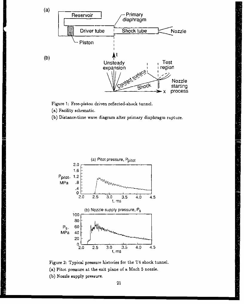
The principal features of a shock tunnel and its operation are shown in Figure 1. The

driver tube, which initially contains low pressure helium, and the shock tube which contains

the test gas are separated by the primary diaphragm. Attached to the downstream end of

the shocktube is a nozzle who,e throat is significantly snalierthan the diaet•,er .f the shock

tube. The test gas is contained by a thin mylar diaphragm which separates the shock tube

from the evacuated tcst region.

The first stage of operation of the T4 facility is the launch of the piston and its acceleration

down the compression tube. The driving force is supplied by the compressed air from the

reservoir. The primary diaphragm, which is typically composed of two sheets of 2mm mild

steel, subsequently bursts at a pressure 56.6MPa. At this point, the helium has been

compressed to 1/60th of its initial volume and is contained in approximately 0.5m of the

compression tube.After diaphragm rupture, helium driver gas expands into the shock-tube and compresses

the low pressure test gas before it. The incident shock travels the length of the shock

tube, reflects from the closed end of the tube and brings the test gas to rest in the nozzle

2

supply region. Operation in this manner is called "tailored" [10] and is shown in the (x-

t) diagram (Figurc 1(b)) by the contact surface coming to rest when intercepted by the

rdflected shock. The compressed test gas is contained in the nozzle supply region in a length

of approximately 0.25 - 0.5m. Ideally, the nozzle supply conditions are maintained as the

reflected shock continuets upstream through the driver gas.

Upon shock reflection, the light secondary diaphragm bursts and some of the compressed

test gas expands into the nozzle. Smith [11] has provided a quasi- one-dimensional model for

the nozzle starting processes.

For combustion studies, the useful test time is terminated by the contamination of the test

gas by the driver gas. The mechanism for this contamination is the bifurcation of the reflected

shock into two weaker oblique shocks near the wall of the tube. This mechanism has been

studied in [12] and has been shown to occur for undertailored conditions at high enthalpies

[13]. For undertailored operation, conditions are such that, when the reflected shock reaches

the helium-air interface, it accelerates into the helium and an expansion propagates into the

nozzle supply gas. With no other influences, the supply region will reach a new equilibrium

but there will be a significant and unavoidable drop in nozzle supply pressure P, shortly

after shock reflection. The expansion of the test gas slug delays the arrival of helium jetting

down the walls of the shock tube and prolongs the useful test time. The approximate time

at which contamination of the test gas is expected to reach the nozzle throat decreases with

increasing stagnation enthalpy, H,, (see, e.g., [1]).

The effect of finite driver siz:. upon the relaxation of P. is also noticeable. Stalker [14]

has suggested a mode of operation where the motion of the piston (after rupture) maintains

approximately constant conditions in the driver tube while nearly 50% of the helium flows

into the shock tube. Following this initial period, of approximately lms, the pressure in the

driver decays rapidly and this decay is transmitted downstream along a (u+ a) characteristic.

The effect of the finite volume of the driver tube is that the the decay in P. may start early

in the test period.

The net result is that the history of the nozzle supply pressure and a representative pitot

pressure at the exit plane of the Mach 5 nozzle will appear as shown in Figure 2. The

pressure transducer measuring P, is located a few centimetres upstream of the reflecting end

of the shock tube. Its trace shows the passage of the incident shock and the arrival of the

reflected shock. Due to transducer rise time and location, the full reflected pressure is not

recorded. Past the peak value, there is a continuous decay in P. due to the combiaed effects

of undertailored operation and driver pressure decay. For helium driver gas and operation

considered here, this decay is typically 25 - 30% during a nominal 0.Sms test time [15]. Note

the delay between the supply pressure trace and the pitot pressure trace. This delay will be

3

used in the normalization procedure discussed in Section 3.5.

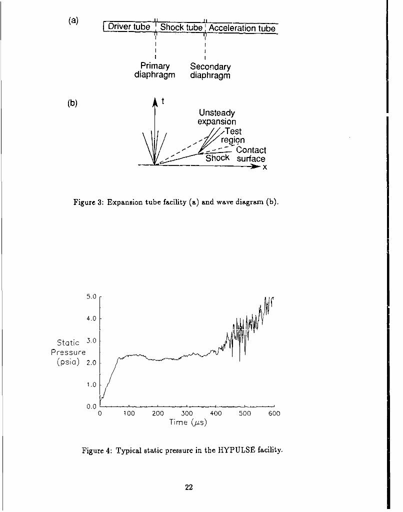
2.2. Expanision Tube

An expansion tube facility consisting of a driver tube (initially containing high pressuredriver gas), a shock tube (containing the test gas) and an acceleration tube (containing low

pressure acceleration gas) is shown schematically in Figure 3. The driver tube and shock

tube are separated by the primary diaphragm and the acceleration tube is separated from

the shock tube by a secondary (and very light) diaphragm. The shock- and acceleration

tubes have the same diameter. Although the HYPULSE facility has a fixed driver tuberather than a free-piston driver, the gas-dynamic processes in the shcck tube are similar.

The operation is initiated by the rupture of the primary diaphragm. High piessure drivergas flows into the shock tube and the incident shock compresses and accelerates the test gas.

On reaching the end of the shock tube, the secondary diaphragm bursts (ideally without

causing disturbance) and the shock-compressed test gas expands into the the low pressure

gas in the acceleration tube. The pressure to which the acceleration gas rises is below the

pressure of the bulk of the shock-compressed test gas and so the downstream portion of the

test gas undergoes an unsteady txpansion to the test flow conditions.

The test time commences after the test-gas/acceieration-gas interface arrives and usually

finishes with the arrival of the downstream end of the unsteady expansion fan. Figure 4

shows a typical history of the static pressure in the test region. The trace shows a rapid rise

due to the shock through the acceleration gas, a slower rise (possibly due to diffuser starting

processes) to the test conditions at approximately 60ts and then roughly constant until the

arrival of the unsteady expansion 400ps later.

3. N1TrUMrrERICAL SIMULATION

The computations of flow through the generic supersonic combustor were made with theLangley Research Center SPARK-2D code. This two-dimensional, elliptic, finite difference

code was developed by J. P. Drummond [5], [6] to integrate the conservation equations for

mass, momentum and energy in a time accurate manner. Since the primary concern is the

temporal development of the combustor flow features, the scope of the modelling was reduced

by considering only laminar flow of a nonreacting test gas and avoiding the fuel injection and

mixing isaues. The effects of transition, turbulence, mixing and chemistry will be examined

in future studies.

4

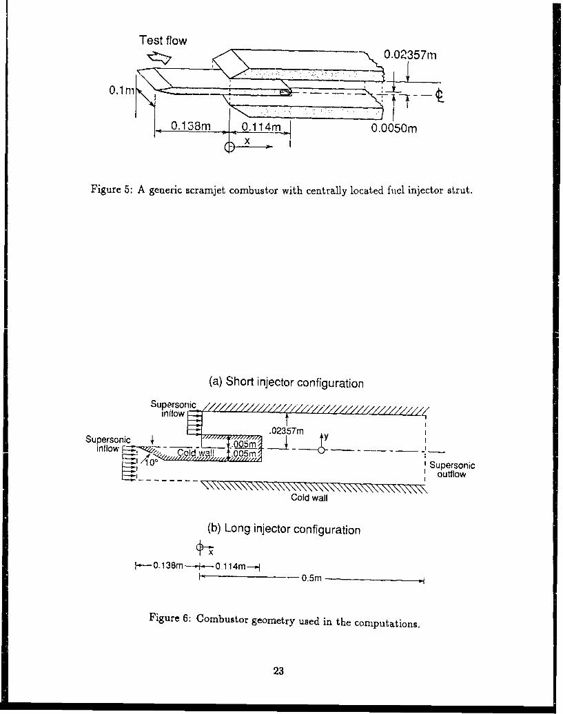
3.1. Combustor Geometry and Boundary Conditions

A generic scramjet combustor, typical of those testcd in the reflected shock tunnel T4[15], is shown in Figure 5. This model consists of the major features of a scramjet combus-

tor, including some form of injector (with an associated wake/mixing region) and a set or

confining walls (with their associated boundary layers).

To perform the two-dimensional computations, the scramjet combustor duct in Figure 5was modelled as shown in Figure 6. Only half of the duct was considereci in the computational

domain. Two classes of calculations were performed which differed in the location of the

inflow boundary. Cases 1,2,3 and 6 with the inflow boundary at the start of the duct walls

(x = 0), have a flow domain as shown at the top of Figure 6. These are called the "short"

injector cases. Cases 4 and 5, with the inflow boundary at the injector strut leading edge

(x = -0.138m), are called the "long" injector cases (Figure 6(b)). Descriptions of the six

cases considered in this study are shown in Table 1.

Boulidary conditions on the wall (at y = 0.02357m) and the surfaces of the injector wereset to zero velocity, zero normal pressure gradient and a fixed temperature T = 300K (i.e.,

cold wall). Cases 4 and 5 included a free boundary along y = 0.02357m for -0.138m < x <

Om. Conditions at the inflow plane were supersonic. The outflow boundary at x = 0.5m

was specified as supersonic with zero gradients in the flow direction. In Cases 1 and 2, the

x-axis downstream of the injector (x > 0.114) was set as a cold wall so as to provide a

situation close to that found in parallel wall injection st'Adies. Cases 3,4,5 and 6 set this line

to be a symmetry plane with zero normal velocity and zero normal gradients for pressute,

temperature, and tangential velocity.

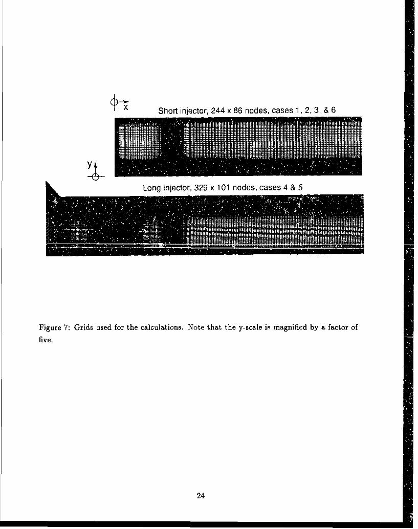
3.2. Qrids

The grids used in the computation are shown in Figure 7. The entire domains, including

the injectors, were included in the grids and during the computation all grid points within

the injector were reset to initial conditions. Each grid consisted of a number of separate

zones in which the nodes were clustered at one or more of the zonal edges so that large flow

gradients near the boundaries and planes defining the injector could be resolved without

excessive computational expense.

The x and y coordinates for the grids used in the short injector cases were independently

generated using one of Roberts' [16] stretching tiansformations. (See also [17], Section 5-b.1).

In each zone there were N + 1 nodes, including the end points, located at

Z = ZA?? + Zb(1 - r), (i)

5I

where4 [(32a)A-f72a] (2)

(2a - 1) [1 + A] '

A= io + 1i) I(3a)

7= J = 0... .N. (4)

Details of the zonal boundaries and stretching parameters are given in Table 2. These

parameters were adjusted until numerical artifacts were eliminated from flow monitors such

as the length of the recirculation region behind the injector (discussed in Section 4.3) and

the position of the recompression shock (discussed in Section 4.4). Note that, for a = 0, the

nodes are clustered close to the z. end of the zone and, for a = 0.5, the nodes are clustered

close to both boundaries.

For the long injector cases, the y-coordinates were generated in a similar manner. How-

ever, the x-coordinates were generated using a compression function due to Thomas et al.

[18]. In each zone there were N + 1 nodes (including end points) specified by Equation 1

andf = 77o rIszQ , 1 , (5)

Siflh(A,JL J

whereA1 + (e- 7o 1(6S= •n i+-r(e---i)770 j (6)

and 770 is the value of 77 at which maximum compression occurs. Details of the zonal bound-

aries and stretching parameters are given in Table 3.

3.3. Initial Conditions and Inflow Conditionls

The initial conditions within the combustor were set to T = 300K, P = 300Fa and zero

velocity so as to approximate the conditions in T4 experiments in which the test section of

the facility is evacuated to approximately 2 Torr.

The inflow conditions were set to approximate the flow in the T4 facility fitted with a

Mach 5 contoured nozzle. The nozzle supply pressure was approximately P5 = 52MPa and

total enthalpy was, H. = 8.4MJ/k.g. Details of the experiment are recorded in [15].

The test flow conditions, both in the shock-reflection region and the nozzle, were com-

puted as quasi-steady flows. The nozzle supply conditions (behind the reflected shock) were

estimated with the FORrRAN program "ESTC" [19] which incorporated an equilibrium

model for air. From the shock reflection conditions, the gas expanded adiabatically (and in

6

chemical equilibrium) to the measured nozzle supply pressure of 52MPa. Using these condi-

tions, the flow at the exit plane of the nozzle was estimated with the quasi-one-dimensional

program "NENZF" [20] in which the test gas consisted of a mixture of the species N2 , N,

02, 0, NO, NO+ and e-. The gas was assumed to be in chemical equilibrium at the nozzle

throat but a finite rate chemistry mode] with 11 reactions was used in the expansion region

of the nozzle.

The "steady" conditions at the end of the nozzle (and inlet to the combustor) were spec-

ified as free-stream velocity 3670mrs-1, a static pressure of 21.5kPa, a static temperature of

1165K, and oxygen and nitrogen mass fractions of 0.2314 and 0.7686 respectively. Although

the NENZF program determined a species mixture that included finite amounts of 0 and

NO, only a nonreacting mixture of 02 and N2 was used in the SPARK-2D computations.

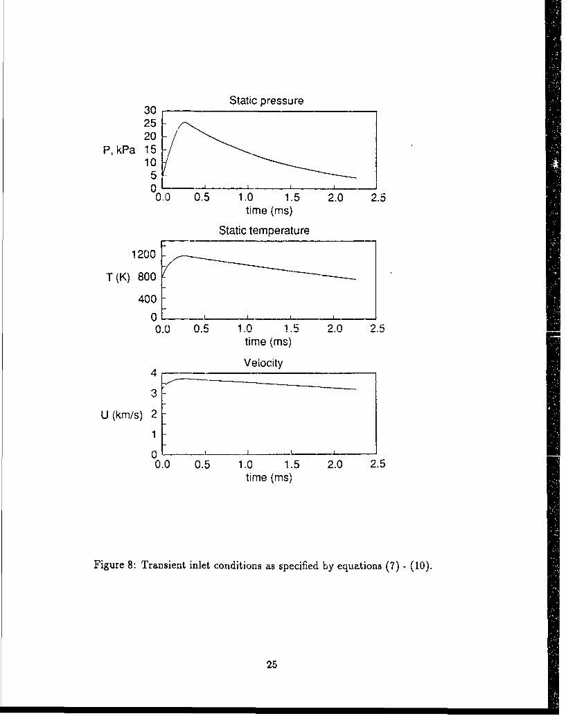
The "transient" inflow was constructed from the nozzle supply pressure trace shown in

Figure 3, assuming a quasi-steady flow and using the ESTC and NENZF codes to compute

the nozzle exit conditions for a number of values of P,. The time evolution of P. was then

approximated by the curve fit

P, = Ppak(0.215 + 4.540t - 22.148t 3 ), 0 < t < 0.28,

= PCaL(ezpO.775(t - 0.28))).0.29 <t < 2.26 (7)

where P,,,k = 62MPa, t is in ms and P, is in MPa. The conditions at the inlet to the

scramjet combustor were then related to P, with the following equations

P,,(kPa) = 0.435P - 1.55, (8)

T,,(K) = 525 .2P.. , 56 , (9)

U,,,(ms-') = 350Tino°333. (10)

The histories of the inlet conditions are shown in Figure 8.

3.4. Numerical Damping

Some difficulty was experienced in starting the solution with such low pressure and large

incident-shock Mach number (which was approximately 10 for Case 1). The difficulty ap-

peared to be caused by the imt .raction of the strong incident shock structure with the newly

forming recompression shock. To get the calculation started, the CFL number was linearly

varied from 0.1 to 0.8 over the first 18000 time steps. For Cases 2,3,4 and 5, the coefficient

for the artificial viscosity terms was set to a constant value of -1.0 while, for Cases 1 and 6, it

was set to -1.2. To faithfully capture heat transfer, temperature smearing was not included.

'1

3.5. Normalization Procedure for Transient Flow

The flow quantities, q(x, t), computed in the transient Cases 2, 3 & 5 were normalized with

upstream reference values to produce equivalent quasi-steady values, 4(x, t). The particular

transformation used, based on the "hypersonic equivalence principle" was

S0q(x, t)(,)=q(Xo, t - Tdea) (I1

where the time delay, Tdelau, was given as the nominal transit time from the reference position

X - XQ (12)

Uin

Essentially this means that individual parcels of fluid were followed downstream through the

combustor and measured quantities were referenced to the parcels' initial states. (See, e.g.,

Section 4.8 of [4].)

4. RESULTS AND DISCUSSION

In previous studies of impulsively started flows [21] [22] [23] [24] one principal result

has been the time taken for the flow to approach steady state. This establishment time

Tr is usually combined with a characteristic velocity, U,, and a length, L,, to form the

dimensionless parameter

UG U're (13)Lc 7

which represents the ratio of the flow establishment time to the tinme for flow to proceed

through the domain. For the flow features in the generic scramjet, such as boundary layers

and recirculation regions, G will have different values. For the impulsively started flow over

a flat plate, where the boundary lavyer is laminar and L, is the distance- from the start of

the plate, G is approximately 3 [21]. When th, boundary layer is turbulent G z 2. For the

wake of a sphere, with L4 as the length of t.h.2 recirculation region, Holden [22] gives G L 30,based on the pressure measurements and G !- 70 based on heat transfer measurements.

In this section, six numerical simulations of the transient flow in a generic scramjet corn-

bustor will be examined with emphasis on the approach to steady state (or quasi-steady state

as determined by the hypersonic equivalence principle). The following parameters will be

used to determine flow establishment times: the boundary layer thicknesses at the end of the

injector strut, the length of the recirculation region, the location of the recompression shock

and, the pressure, heat flux and shear stress on the y = 0.02357m wall. The computation

of the flow development for each of the cases was continued to a time of approximately lrns

which is typical of the flow time in the current generation of pulsed-flow facilities.

8

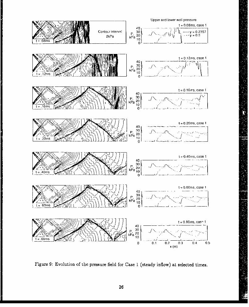
4.1. Overview of the Sn'utions

Figures 9 anr' 10 show the pressure fields for the short injector geometry with steady

inflow (Case 1) and transient inflow (Case 2) rcspectively. Contour spacing is 2kPa. These

figures highlight the similarity between the steady inflow and the transient inflow solutions.

The pressure distributions along the y = 0 and y = 0.02357m walls are shown on the rigbt

side of each figure. Note that the stretching of the y-coordinate (by a factor of 5) changes

the appearance of the shock and Mach angles.

At the start of the duct, there are a pair of weak shocks generated by the initially rapid

growth of the boundary layer on the duct walls. Although not evident in the pressure field

plots, boundary layers develop along the upper wall and the injector surface. The boundary

layer on the injector separates at the step (x = 0.114m) and reattaches to the y = 0

boundary some distance downstream. The expansion from the corner of the injector, and

the recompression shock formed near the end of the recirculation zone are clearly visible for

both cases. Subsequent reflections of the recompression shock from the duct walls can be

seen for t > 0.2ms.

The initial shock structure sweeping through the duct for t < 0.16ms is composed of an

incident shock propagating downstream through the quiescent gas, a contact discontinuity

separating the initial duct gas and the incoming test gas, and an upstream-facing shock

decelerating the incoming test gas. Both the second-order and fourth-order MacCormack

schemes experienced some difficulty with this strong shock structure and numerical oscilla-

tions are evident in the solutions for t < 0.20ms. However, it is expected that the solutions

are reliable at later times.

The incident-shock position was identified as the point at which the wall pressure rose

from (the initial value of) 300Pa to 80OPa. The position was recorded every 10szs and the

data points were then fitted with the straight line

S= v(t - to). (14)

The values of v and to are given in Table 4. In all cases, the shock speed was virtually

constant throughout the flow domain. However, the transient inflow cases (2,3 and 5) had

a lower incident-shock speed than the steady inflow cases. For Cases 1 and 6, the position

of the upstream-facing shock was identified as the point where the wall pressure crossed a

35kPa threshold. The velocities for this shock are a1.so given in Table 4.

As shown by the pressure contour plots and the wall pressure plots in Figures 9 and

10, the overall flow features of both steady inflow and transient inflow cases are similar.

Although the starting shock structure took longer to exit the duct for the transient inflow

(Case 2), the major steady-state features such as the boundary-layer interaction shocks, the

9

expansion fan and the recompression shock are in vi-tually the same places. The principal

difference seems to be the average level of the duct pressure which can be seen relaxing in

the wall pressure plots of Figure 10.

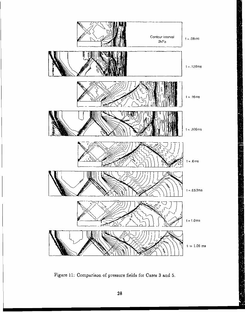
The effect of including the complete inijector strut in the computational model can be

seen in Figure 11, which shows a few frames from Cases 3 and 5. The frames are placed

back to back and the times have been chosen to show approximately the same stages of

development. However, the instantaneous inflow conditions are not exactly the same in each

pair of frames. The major differences are the strong rhock and expansion propagating from

the front of the long injector. Also, the shock propagating from the leading edge of the

y = 0.02357m wall is stronger than the boundary-layer interaction shocks seen in the short

injector simulations. After reflecting from the injector strut and then the duct wall, this

leading-edge shock interacts with the expansion fan propagating from the base of the strut.

Since there is only a small difference between the long-injector and short-injector simula-

tions, the following discussion will concentrate on the details of the short-injector simulations.

4.2. Injector-Strut Boundary Layer

For the short injector simulations, the boundary layer along the strut surface closely

approximates the ideal flat-plate boundary layer, the main difference being the boundary-

layer interaction shock striking the strut surface at x "• 0.09m. This weak shock did riot seem

to affect the flow profiles within the boundary layer at the end of the strut (x = 0.1147n)

where the following thicknesses were calculated:

"* total boundary layer thicknes:, 6; the y-distance from the strut surface to 0.99 of the

local free-stream velocity ui,,

"* the displacement thickness

1* (i- , (15)

"* the momentum thickness

0= $Q-(1 . (16)Peue \ ,

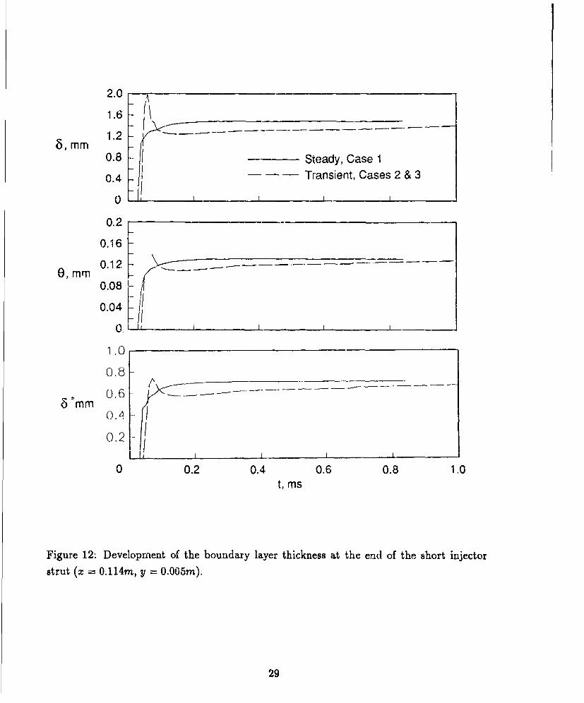
The temporal development of 6, 8" and 0 is shown in Figure 12. For the steady inflow,

the thicknesses approach to within 2% of steady stale values by t = 0.23 - 0.26ms. If the

approach to steady state begins with the passage of the upstream-facing shock, these times

give G L 7 which is roughly double the value expected for a laminar boundarv layer in shock-

tube flow [21]. This result seems to indicate that the incident shock structure, including the

10

contact surface and the upstream facing shock, interferes with the establishment processes

and delays the approach to steady state.

The steady value of 8 = 1.49mm is close to the value of 1.45mm obtained with the"reference temperature" relations of Eckert [25] and Equation (7.53) in White [26]. This

agreement provides some confidence that the viscous effects have been adequately resolved.

Also, the flat plate transition data from He & Morgan [27] indicate that transition to a

turbulent boundary layer would be expected after a distance of approximately 0.25m.

For the transient inflow cases, the approach to steady state is qualitatively different and,

at late times, there is a slight growth in each of the thicknesses as a consequence of the

relaxation of the free-stream pressure (and hence density).

4.3. Recirculation Region

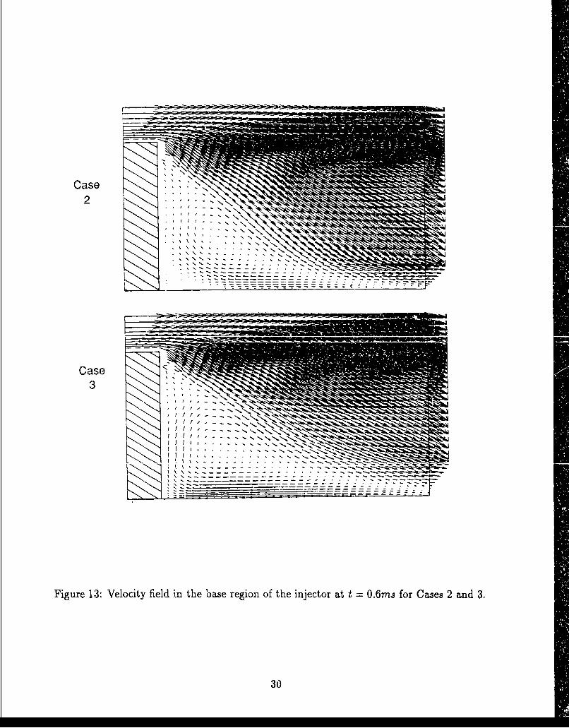
The form of the velocity field in the recirculation region at the base of the strut appeared

to be insensitive to the transient inflow. Figure 13 shows the velocity field in the recirculation

region for Cases 2 and 3. The symmetry plane boundary condition in Case 3 allows a stronger

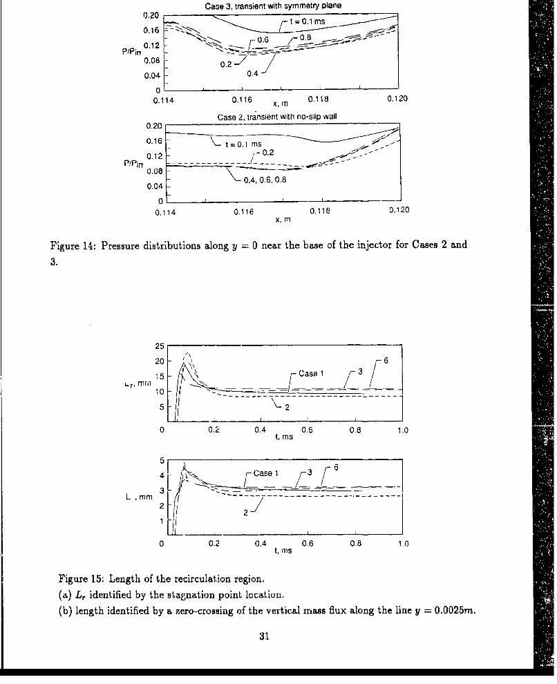
vortex to form closer to the strut base. The pressures along the y = 0 line in the recirculation

region are shown in Figure 14 at selected times.

The length of the recirculation region, as measured by the position of the stagnation point

near the y = 0 boundary, is showr, i, Figure 15. At late times, both the steady inflow and the

relaxing inflow traces reach steady values. The steady state lengths are L, *= 9.5, 8.3, 10.1

and 10.8mm for Cases 1,2,3 and 6 respectively, which means that (a) the symmetry plane

cases have longer recirculation zones than the solid wall cases and (b) the transient inflow

case.- have slightly shorter lengths than their steady inflow counterparts. Based on L, for

steady inflow, the base flow establishes in a dimensionless time G z- 146 (t = 0.419ms) for

the sob1d wall (Case 1) and G 9 .3 (t = 0.283rn.A) for the symmetry plane (Case 6).

Also shown in Figure 15 is the length of the recirculation region along the line y =

0.0025m which is half way up the base of the strut. This length was determined by computing

the vertical mass flux

'il puudx, (17)

and finding the x-location where rhv became zero. This measure showed the same trends

as the stagnation point measurement except that G t• 64 (t = 0.229ms) for the symmetry

plane (Case 6).

4.4. Recompression Shock

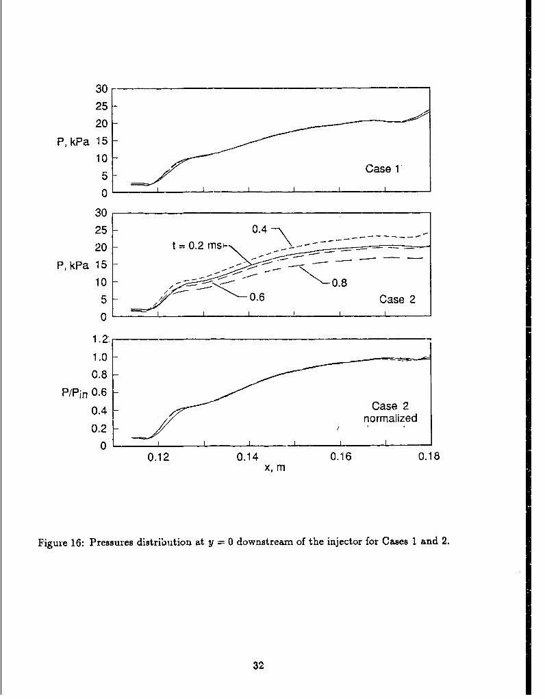
Figure 16 shows the pressure distributions along the y = 0 plane for Cases 1 and 2.

11

The recompression bhock is rather smeared and appears as the gradual pressure rise from

x ýa 0.1 2m to x - 0.13rn. Observe that the pressure distributions for the transient inflow

(Case 2) collapse onto the one curve when they are normalized using the procedure discussed

in Section 3.5.

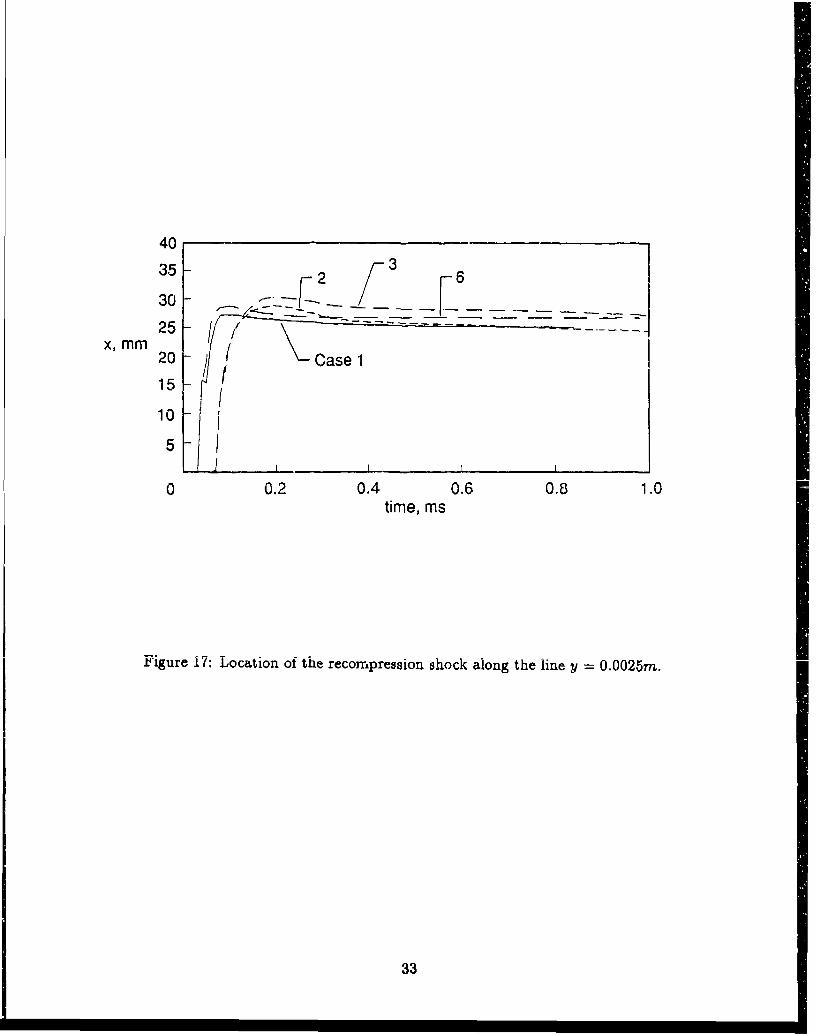
The shock position along a line through the midpoint of the strut base (y = 0.0025m) is

plotted against time in Figure 17. The shock position was taken to be the grid location at

which the pressure rises to 25% of the inlet pressure. Based on the length of the recirculation

zone the nondimensional cstablishment time G "" 140 (t = 0.402rns) and G '2_ 80 (t =

0.273ms) for Cases 1 aad 6 respectively.

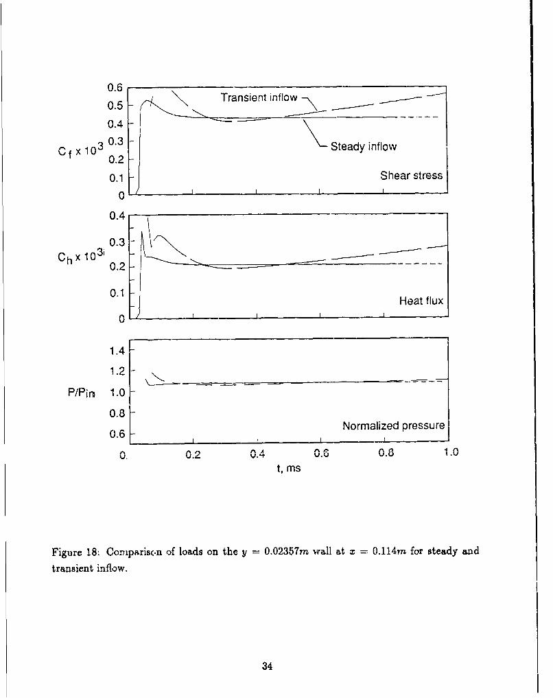
4.5. Wall Loads

The shear stress and heaL flux were monitored at selected points along the y 0.02357m

wall. The shear stress coeff..:ient is glven by

1 - 2 (18)"j PinUin

and the heat flux by the Stanton number

Ch = p 9u inCp(Ta, - (19)

where the normal derivatives of the velocity and temperature were approximated by differ-

ences at the first node off the wall. The viscosity was evaluated at the wall temperature using

Sutherland's formula and pin and un are inlet conditions computed with the true delay spec-

ified in Equation (12). Thermal conductivity k was obtained assuming Cp = 1004J/kg/K

and Prandtl number Pr =_ p/k = 0.71. The adiabatic wall temperature was obtained

from

=,1 1+ / 2 M ] (20)

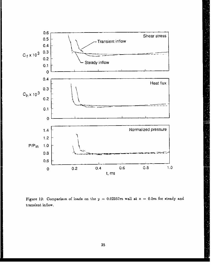
The development of these parameters at x = 0.114m and x = 0.5m, is shown in Figures 18

and 19 respectively. Results for the steady inflow cases exhibit an approach to steady state

at both locations. The normalization of the transient inflow measurements is not entirely

successful as the values of both Cf and Ch settle to a constant rate of growth after some

start-up period.

Normalized pressure histories at x = 0.114m and 0.5077 wall are shown in Figures 18(c)

and 19(c) for completeness. There is only a slight variation in the traces for the two transient

inflow cases indicating that the normalization works well for pressures. The slight variation

may be caused by the use of the constant value Uc, = 3670ns-1 in Equation (12).

12

4.6. (x,t)-Diagrams

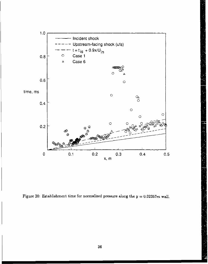
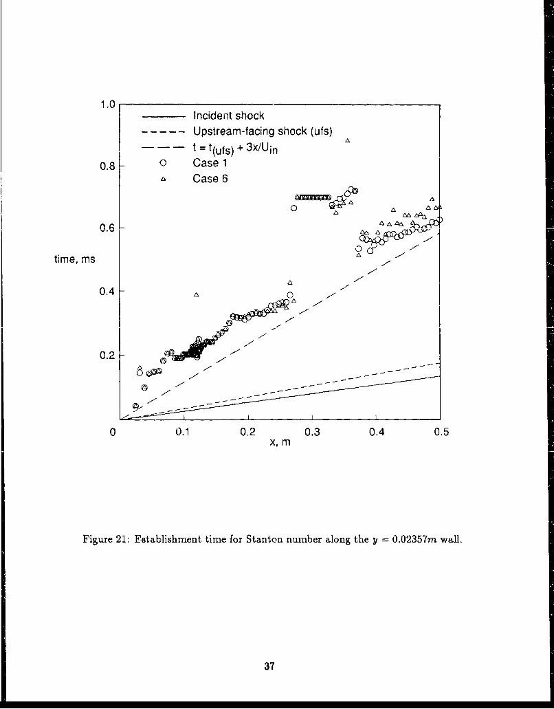
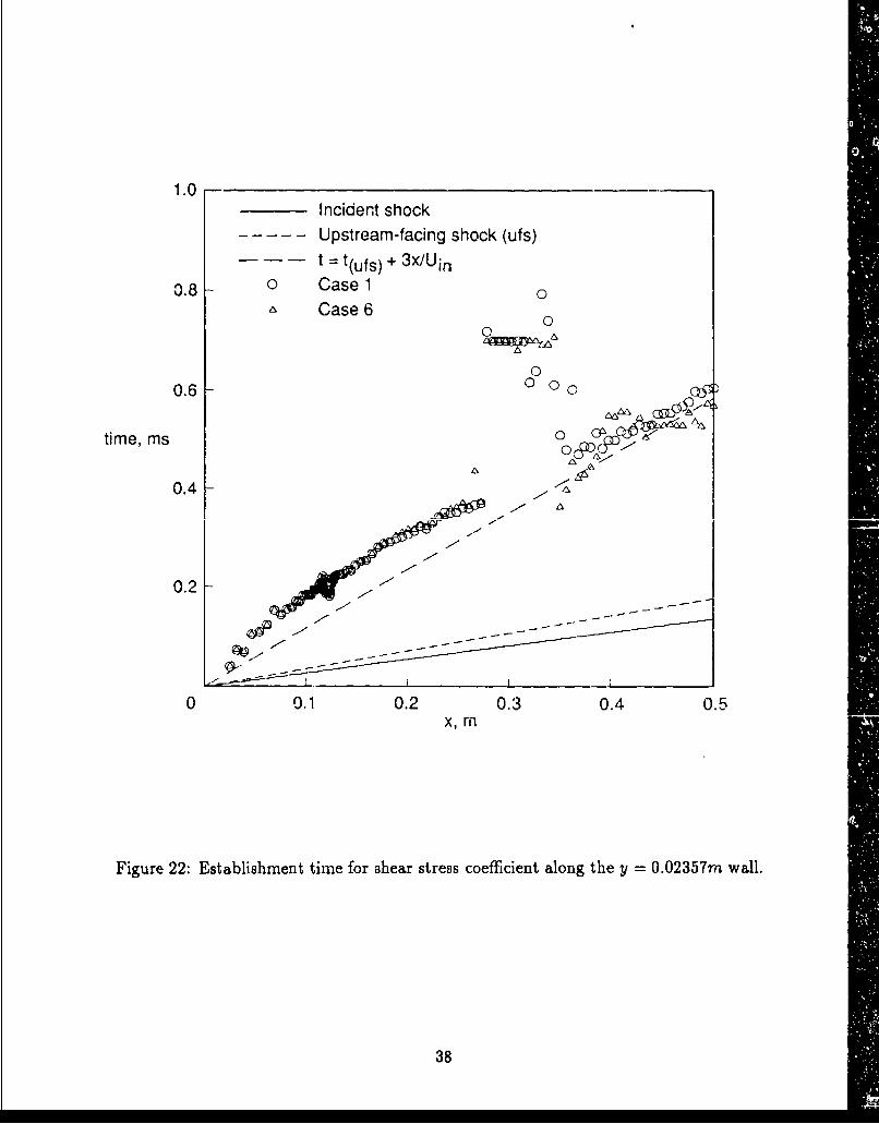
The time for wall pressure, shear stress and heat transfer to reach steady state at a number

of x-locations along the y = 0.02357m wall is shown in Figures 20, 21 and 22 respectively.An average of each quantity between times t = 0.7ms and 0.8ms was used as the steady

value and the settling time t, detcrmined such that the flow quantity remains within 2% of

the steady value for t, < t < 0.ms. The establishment time is then given as T. = te. - tul,

where t,,f is the arrival time of the upstream-facing shock. Only the steady inflow cases (1

and 6) are considered, since a consistent establishment criterion was not available for the

transient inflow cases.

The wall pressure generally settles more nuickly than shear stress or heat transfer and -

has a dimensionless establishment time of G = r-Ucix •- 0.9 for x > 0.2m. However, the

establishment is significantly delayed where the relatively weak boundary-layer-interaction

shocks strike the wall at x Ž- 0.09m. and 0.18m. The pressure measurement does not settle

at all where the relatively strong recompression shock strikes the wall at x •_ 0.3m.

The establishment times for the shear stress are nearly the same as those for the heat

transfer and, for x > 0.4m, can be approximated by G !- 3. A similar delay after the passage

of the starting pulse was observed in the experimental measurements of East et al. [24]. For

x < 0.3, the delay beyond the flat plate value of G L- 3 is significant.

5. CONCLUSION

In order to study the establishment of the major flow features in a generic scramjet

combustor, several numerical simulations were analysed. Of particular interest was the

effect of a transient relaxing inflow condition as found in a reflected-shock tunnel which has

been operated in an undertailored mode.

From the numerical point of view, the simulations were particularly demanding and much

of the interesting phenomena (such as turbulent mixing and chemistry) was omitted from

these simulations. These issues will be addressed in a future study. The finite-difference

scheme generally performed well but encountered difficulty with the very strong shock inter-

actions and tended to produce oscillatory solutions at early times. With an incident-shock

Mach number of approximately 10, these oscillations were not unexpected. An "upwinding"scheme (available in another version of the code) may better cope with the strong shocks.

From the experimental point of view, it appears that the correlations available in theliterature are adequate for predicting the establishment times for the flow features of the

model if the inflow conditions are steady and allowance is made for the passage of the starting

pulse [24]. For the relaxing flow, there are perturbations outside the 2% error band for a

13

significantly longer time but these perturbations are probably umaller than the measurement

uncertainty in the shock tunnel experiment. Hence, relaxing test flow with a duration of the

order of a few hundred microseconds is probably adequate for establishing flow in moderate

sized scramjet models if the recirculating zones are not too large. The establishment time

for turbulent jet mixing in the presence of combustion needs to be examined.

The effect of the relaxing inflow conditions of the undertailored reflected-shock tunnel

seem not to affect the overall pressure fields within the model nor the length of the recircu-

lation region to any great extent. However, the relaxing flow does affect features such as the

heat transfer and wall shear stress. It may also be expected to affect the chemical reaction

rates which will scale as pL, and p2L, for two-body and three-body reactions respectively.

14

References

[1] R. I. Stalker. Hypervelocity aerodynamics with chemical nonequilibrium. Annuol Re-

view of Fluid Mechanics, 21:37-60, 1989.

[2] J P. Drummond, M. H. Carpenter, D. W. Riggins, and M. S. Adams. Mixing enhance-

ment in a supersonic combustor. AIAA Paper 89-2794, 1989.

[3] G. B. Noitham and et al. Evaluation of parallel injector configurations for supersonic

combustion. ALAA Paper 89-2525, 1989.

[4] J. D. Anderson. Hypersonic and High Temperature Gas Dynamics. McGraw-Hill, New

York, 1989.

[5] J. P. Drummond, R. C_ Rogers, and M. Y. Hussaini. A detailed numerical model of a

supersonic reacting mixing layer. AIAA Paper 86-1427, 1985.

[6] J. P. Drummond. A two-dimensional numerical simulation of a supersonic, chemically

reacting mixing layer. NASA Technical Memorandum 4055, 1988.

[7] PR. C. Rogers and E. H. Weidner. Numerical analysis of the transient flow from a shock

tunnel facility. AIAA Paper 88-3261, 1988.

[8] R. G. Morgan and et al. Shock tunnel studies of scramjet phenomena. NASA Contractor

Report 181721, 1988.

[9] J. Tamagno and et al. Results of preliminary calibration tests in the gasl hypulse facility.

GASL Technical Report 308, General Applied Science Laboratories, Ronkonkoma, New

York, 1989.

[10] C. E. Wittliff, M. R. Wilson, and A. Hertzberg. The tailored-interface hypersonic shock

tunnel. J. Aerospace Sci., 26:219-228, 1959.

[1.1] C. E. Smith. The starting process in a hypersonic nozzle. Journal of Fluid Mechanice,

24:625-640, 1966.

[12] L. Davies and J. L. Wilson. Influence of reflected shock and boundary-layer interaction

on shock-tube flows. The Physics of Fluids Supplement 1, 1969.

[13] R. J. Stalker and K. C. A. Crane. Driver gas contamination in a high enthalpy reflected

sh'ck tunnel. AIAA. Journal, 16(3):277-279, 1978.

15

[14] R. J. Stalker. A. study of the free-piston shock tunnel. AIAA Jou -nal, 5(12):2160-2165,

1967.

[15] P. A. Jacobs and et al. Preliminary calibration of a generic scramjet combustor. De-

partment of Mechanical Engineering Report in preparation, Uuiver.ity of Queensland,

1990.

[16] G. 0. Roberts. Computational meshes for boundary layer probhems. In Lecture Notes

in Physics, 8, pages 171-177. Springer-Verlag, 1971.

[17] D. A. Anderson, J. C. Tannehill, and R. H. Pletcher. Computational Fluid Mechanics

and Heat Transfer. Hemisphere, New York, 1984.

[18] P. D. Thomas, M. Vinokur, R. Bastianon, and R. J. Conti. Numerical solution for the

three-dimensional hypersonic flow field of a blunt delta body. AIAA Journal, 10:887-

894, 1972.

[19] M. K. McIntosh. Computer program for the numerical calculation of frozen and equi-

librium conditions in shock tunnels. Technical report, Australian National University,

1968.

[20] J. A. Lordi, R. E. Mates, and J. R. Moselle. Computer program for the numerical solu-

tion of nonequilibrium expansions of reacting gas mixtures. NASA Contractor Report

472, 1966.

[21.] W. R. Davies and L. Bernstein. Heat transfer and transition to turbulence in the

shock-induced boundary layer on a senmi-infinite flat plate. Journal of Fluid Mechanics,

36(1):87-112, 1969.

[22] M. S. Holden. Establishment time of laminar separated flows. AIAA Journal,

9(11):2296-2298, 1971.

[23] E. J. Felderman. Heat transfer and shear stress in the shock-induced unsteady boundary

layer on a flat plate. AIAA Journal, 6(3):408-412, 1968.

[24] R. A. East, R. J. Stalker, and J. P. Baird. Measurements of heat transfer to a flat plate

in a dissociated high-enthalpy laminar air flow. Journal of Fluid Mechanics, 97(4):673-

699, 1980.

[25] E. R. G. Eckert. Engineering relations for friction and heat transfer to surfaces in high

velocity flow. Journal of the Aeronautical Sciences, 22(8):585-587, 1955.

16

[26] F. M. White. Viscous Fluid Flow. McGraw-Hill, New York, 1974.

[27] Y. He and R. G. Morgan. Traniition of compressible high enthalpy boundary layer flowover a flat plate. In Tenth Australiasian Fluid Mechanics Conference, Melbourne., 1989.

17

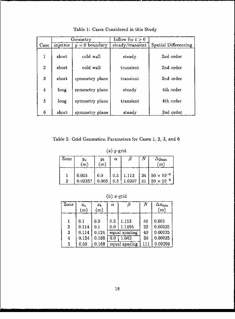
Table 1: Cases Considered in this Study

Geometry Inflow for t > 0Case injector y = 0 boundary steady/transient Spatial Differencing

1 short cold wall steady 2nd order

2 short cold wall transient 2nd order

3 short symmetry plane transient 2nd order

4 long symmetry plane steady 4th order

5 long symmetry plane transient 4th order

6 short symmetry plane steady 2nd order

Table 2: Grid Generation Parameters for Cases 1, 2, 3, and 6

(a) y-grid

Zone Ya Yb a /3 N Ay,,n(m) (m) (m)

1 0.005 0.0 0.5 1.113 34 50 x 10-s2 0.02357 0.005 0.5 1.0307 51 50 X 10-6

(b) x-grid

"Zone x, Xb a 3 N Ax, 1, 1(m) (m) ___ (m)

I

1 0.1 0.0 10.5 1.153 40 0.0012 0.114 0.1 0.0 1.1495 22 0.000253 0.114 0.124 equal spacing 40 0.000254 0.124 0.168 TT 1.042 30 0.000255 0.50 0.168 1 equal spacing 111 0.00299

18

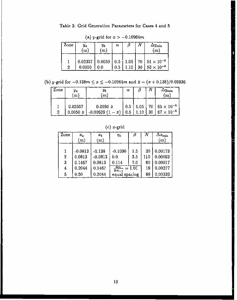
Table 3: Grid Generation Parameters for Cases 4 and 5

(a) y-grid for x > -0.10964m

Zone Ya Yb a N(M) (M) (M)

1 0.02357 0.0050 0.5 1.05 70 51 x 10-62 0.0050 0.0 0.5 1.10 30 53 x 10-6

(b) y-grid for -0.138m < x < -0.10964m and c = (x + 0.138)/0.02836

[Zone -b A a -N AN u(M) (M) __ . (m)

1 0.02357 0.0050 ft 0.5 1.05 70 65 x 10-6

2 0.0050 Z -0.00639 (1 - t) 0.5 1.10 30 67 x 10-6

(c) x-grid

Zone 11 Xb 77o- N I A N1 xwjn(m) (m) __ _ . _ (n)

1 -0.0813 -0.138 -0.1096 1.5 30 0.001732 0.0813 -0.0813 0.0 3.5 110 0.000933 0.1467 0.0813 0.114 7.0 80 0.000174 0.2044 0.1467 [ = 1.01 19 0.002775 0.50 0.2044 equal spacing 89 0.00332

19

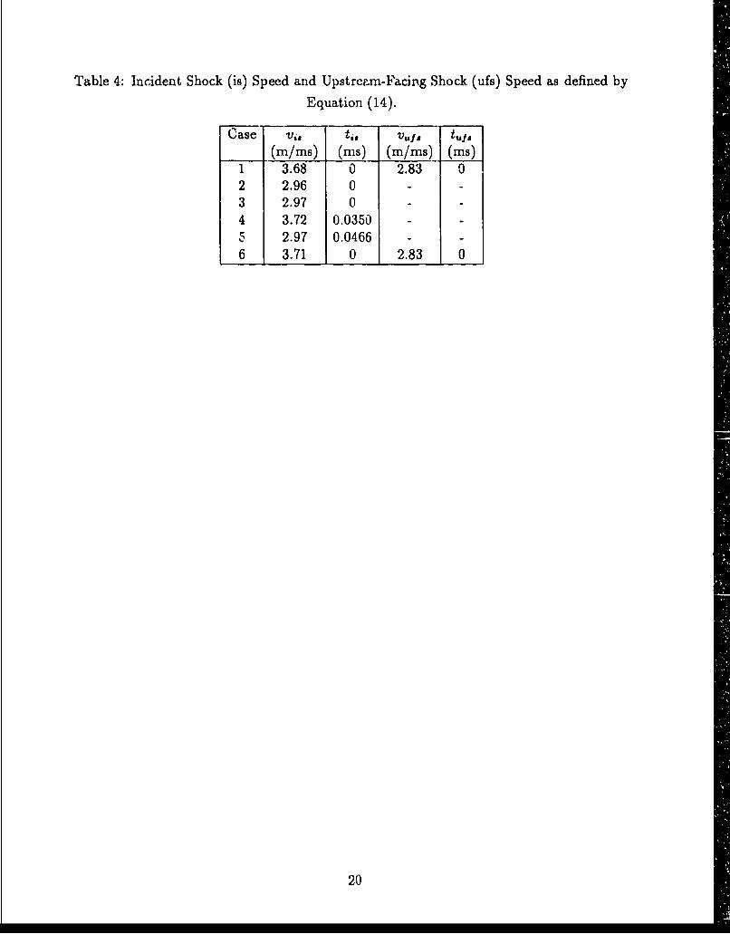
Table 4: Incident Shock (is) Speed and Upstrearm-Facing Shock (ufs) Speed as defined by

Equation (14).

Case vi, ti, V2) a tuf a(m/ms) (nis) (m/ms) (ms)

1 3.68 0 2.83 02 2.96 0 - -

3 2.97 0 - -

4 3.72 0.0350 - -

5 2.97 0.0466 - -

6 3.71 0 2.83 0

20

(a) i , Primary

diaphragm

Drivtube Shocktub~e _Nozzle

SPiston

(b) 4tUnsteady Testexpansion i region

CZ1 I .

Nozzlestarting-ýiox process

Figure 1: Free-piston driven reflected-shock tunnel.

(a) Facility schematic.

(b) Distance-time wave diagram after primary diaphragm rupture.

(a) Pitot pressure, Ppitot2.01.6

Ppilot, 1.2 VMPa .8 V

.4 - I0 L •I, iI-

2.0 2.5 3.0 3.5 4.0 4.5t, ms

Of (b) Nozzle supply pressure, Ps

Ps, 60

20 -

2.0 2.5 3.0 3.5 4.0 4.5t, ms

Figure 2: Typical pressure histories for the T4 shock tunnel.

(a) Pitot pressure at the exit plane of a Mach 5 nozzle.

(b) Nozzle supply pressure.

21

(a) ','rver tube Shock tube' Acceleration tubeII Ii

Primary Secondarydiaphragm diaphragm

(b) t

Unsteadyexpansion

,,Testregion/ [/ .- Ž•Contact

_.• - -Shock surface

Figure 3: Expansion tube facility (a) and wave diagram (b).

5.0y

4.0 IA

static 3.0Pressure

(psia) 2.0

1.0

0.0 . ,

0 100 200 300 400 500 600Time (/•s)

Figure 4: Typical static pressure in the HYPULSE facility.

22

Test flowO,0.02357m

0.138m 0.114mrn 0.0050m

Figure 5: A generic scramjet combustor with centrally located fuel injector strut.

(a) Short injector configuration

Supersonic z

Supersonic 4 , .02357m"Supersonc • __ .I005m .inflow F- , ;. - • d- - -

05m* -ý1 Supersonic

outflow

Cold wall

(b) Long injector configuration

I---0. 138m -- 0. 114m •-I'• ~ 0.5m -

Figure 6: Combustor geometry used in the computations.

23

(•X Short injector, 244 x 86 nodes, cases 1, 2, 3, & 6

Long injector, 329 x 101 nodes, cases 4 & 5

Figure 7: Grids ased for the calculations. Note that the y-scale is magnified by a factor of

five.

24

Static pressure30

252 0 _

P, kPa 15105.0 I_ I

0.0 0.5 1.0 1.5 2.0 2.5time (ms)

Static temperature

1200

T (K) 800

400

0.0 0.5 1.0 1.5 2.0 2.5time (ms)

Veiocity4

U (km/s) 2

1

0.0 0.5 1.0 1.5 2.0 2.5time (ms)

Figure 8: Transient inlet conditions as specified by equations (7) - (10).

25

Upper and lower wali pressure

t= 0.08ms, case 140;

Contour interval 30 R2/-\ _ ., -0.2 5 -2kPa K~a O 20 0 0 "J __

O08ms 100

t ;0.12rns. case 140

__ 0 L~ -i - I 2

t=0.~is cas 1040

t =0 O.6ms, case 1

S, - I ....7~3 V7J__

4 .0 __.j _ ,.N-- __-._ = 0---__, case _~~10t k1a 1 S -j t

I___ 0.20ms, case 1

t = .- 0 ns-Y[/

.6Oms ).) I .f .• I .6L -~A ,30. . ..... .. .J 0 I<t = OB0ms, case 1

,'__'kpa 20I .4mS' kifl. 101 _ ~ - -

0 0t1 0? 0.3 0.4 0.5 I

x (in)

Figure 9: Evolution of the pressure field for Case 1 (steady inflow) at selected times.• :_

26 2

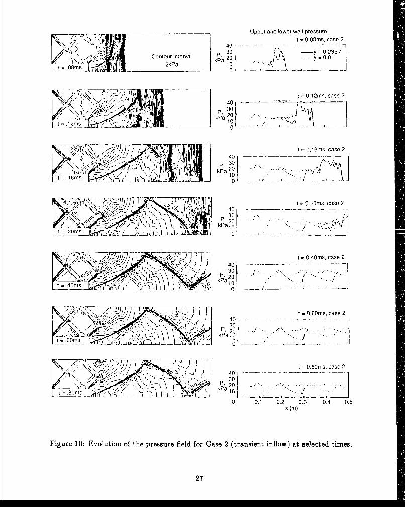
Upper and lower wall pressureI0.O8ms, case 2

Contour interval k 3a 0 -Y 7y 0.05

2kPaka

6 t= 0.l12ms, case 2401___ _ _

ka20Pa3 0

f i t =0. 1 6ms, case 2

40

P 30 /.--- i.- c~'~ ~20

LI2tr5~i.liC i. o kP'a 10

A 777iU:72s* case 2___ 72 ' kP40 -

30

r- J 2h~~r t =0.48Os, case 2

T,~f kPa230 =.0 0.1 0. 0. 0.4 0.

220

>0

2kPa

t.1 26mns

t .26ms

~TT 7 -I -

L~ t=.6nis

t =.653ms

- 7-

t =1.06 Ma

Figure 11. Comparison of pressure fields for Cases 3 and 5.

28

2.0

1.6 _

1.2

0.8 Steady, Case 1

0.4 - - - Transient, Cases 2 & 3

0.20.16

0.12 - ------

0.08 L

0.04

0 I I I I I I

1.0

0.8

•3 mram O. 0.6 _.. ---......

"MM 0.4 10.2

I _ 1 I I I ,

0 0.2 0.4 0.6 0.8 1.0t, ms

Figure 12: Development of the boundary layer thickness at the end of the short injector

strut (x = 0.114m, y = 0.005m).

29

Case2

Case

Figure 13: Velocity field in the base region of the injector at t 0.6ms for Cases 2 and 3.

30

Case 3, transient with symmetry plane0.20 _F t = 0 .1 m s

P/Pin 0.120o.08 o.0----"2

0.04 0.4

0 ---- --- --- --L ------ -- -----

0.114 0.116 Xn 0.118 0.120

Case 2, transient with no-slip wall0.200.16 t = 0.1 ms

0.12 / -0.2P /P in - . . . . .----------

0.08 -

0.04 -0.4, 0.6, 0.8

0 I I -- ]

0.114 0.116 0.118 0.120X, m

Figure 14: Pressure distributions along y = 0 near the base of the injector for Cases 2 and

3.

25 ]__

20 - 6

15 Case 1 3Lr, mrw 1 )/ ri --- -------

5 11,-2 15 / I rI I0 0.2 0.4 0.6 0.8 1.0

t, ms

4 Case 16

L Im ~ - --------------- _----3 h-- ----------

L ,mm If

2

0 0.2 0.4 0.6 0.8 1.0t, ils L •.

Figure 15: Length of the recirculation region.

(a) L- identified by the stagnation point location.

(b) length identified by a zero-crossing of the vertical mass flux along the line y = 0.0025m.

31

30 - _ _ _ _ _ _ _ _ _ _ _

25

20

P, kPa 1510

Case 1'0

30

25 0.4-\- -

P, kPa 0.8

5 0.6Case 2

0

1.2.

1.0

0.8

P/Pin 0.60.4 Case 2

normalized

0.12 0.14 0.16 0.18X, m

Figure 16: Pressures distribution at y =0 downstream of the injector for Cases 1 and 2.

32

40

35 23630

x, mm '20m /-Case 12

15

10

51

0 0.2 0.4 0.6 0.8 1.0time, ms

Figure 17: Location of the recormpression shock along the line y = 0.0025m.

33

0.6

0.5 Transient inflow

0.4 -

x 103 0.3 - Steady inflowCfx 030.2

0.1 Shear stress

010.40.3 -

Ch x 103i 0-

0.2

0. Heat flux

0 I

1.4 F1.2 F

P/Pir 1.01-

0.8 -

0.6 - Normalized pressure[ I I

O.0.2 v0.+.u ".J,)

t, ms

Figure 18: Cornparisc.n of loads on the y = 0.02357m wall at x = 0.114m for steady and

transient inflow.

34

0.4 -Transient inflow

CfXl10 3 0.3 __ -

0.2

0.1 Steady inf low

0

0.4_____Heat flux

0.3

Chx 103

0.2-

0.1

0 I I I

1.4 Normalized pressure

1.2

P/Pin, 1.0

0.8 -_"

0.6

0 0.2 0.4 0.6 0.8 1.0t, ms

Figure 19: Comparison of loads on the yg = 0.02357m wall at x = 0.5m for steady and

transient inflow.

35

1.0Incident shock

Upstream-facing shock (ufs)t = t is + 0"9x/Uin.

0.8 0 Case 1

Case 6

0 A

0.6 0

time, ms

00.4

0

0 0

0 0

0 0.1 0.2 0.3 0.4 0.5X, m

Figure 20: Establishment time for normalized pressure along the y = 0.02357m wall.

36

1.0Incident shock

Upstream-facing shock (ufs)

t = t(ufs) + 3X/Uin

0.8 o Case 1, Case 6

0 • a

A A -1,4 4'Aj

0.6 •0

time, ms A

A A "

0.4 A 0

0.2 -

0 0.1 0.2 0.3 0.4 0.5x, m

Figure 21: Establishment time for Stanton number along the y = 0.02357m wall.

37

1.0 -____________________Incident shock

- - -- Upstream-facing shock (ufs)t=t(ufS)+3XUin

3.8 - 0 Case 1 0Case 6

0

0

0.6 -0 00

6d"-

AI-

time, ms 0 01.

0.2

0 0.1 0.2 0.3 0.4 0.5x, m

Figure 22: Establishment time for shear stress coefficient along the y 0.02357m wall.

38