ibm z/os v2r2 performance and availability topics
TRANSCRIPT

© 2015 IBM CorporationITSO-1
Welcome
DAY 2
Performance & Availability
© 2015 IBM CorporationITSO-2
Topics Covered
• Software Pricing and You• IBM z13 Performance• IBM z13 SIMD• IBM z13 SMT• IBM z13 Coupling• Erase-on-Scratch Enhancements in z/OS 2.1• zEnterprise Data Compression (zEDC)• Planned Outage Considerations
• Focus of all sections is on price/performance – getting the maximum value from your investment in System z.
© 2015 IBM CorporationITSO-3
Agenda
• 09:00 Start
• 10:30 – 10:45 Coffee Break
• 12:30 – 13:30 Lunch
• 14:45 – 15:00 Coffee Break
• 17:00 Finish!

© 2015 IBM CorporationITSO-44
The following are trademarks of the International Business Machines Corporation in the United States, other countries, or both.
The following are trademarks or registered trademarks of other companies.
* All other products may be trademarks or registered trademarks of their respective companies.
Notes: Performance is in Internal Throughput Rate (ITR) ratio based on measurements and projections using standard IBM benchmarks in a controlled environment. The actual throughput that any user will experience will vary depending upon considerations such as the amount of multiprogramming in the user's job stream, the I/O configuration, the storage configuration, and the workload processed. Therefore, no assurance can be given that an individual user will achieve throughput improvements equivalent to the performance ratios stated here. IBM hardware products are manufactured from new parts, or new and serviceable used parts. Regardless, our warranty terms apply.All customer examples cited or described in this presentation are presented as illustrations of the manner in which some customers have used IBM products and the results they may have achieved. Actual environmental costs and performance characteristics will vary depending on individual customer configurations and conditions.This publication was produced in the United States. IBM may not offer the products, services or features discussed in this document in other countries, and the information may be subject to change without notice. Consult your local IBM business contact for information on the product or services available in your area.All statements regarding IBM's future direction and intent are subject to change or withdrawal without notice, and represent goals and objectives only.Information about non-IBM products is obtained from the manufacturers of those products or their published announcements. IBM has not tested those products and cannot confirm the performance, compatibility, or any other claims related to non-IBM products. Questions on the capabilities of non-IBM products should be addressed to the suppliers of those products.Prices subject to change without notice. Contact your IBM representative or Business Partner for the most current pricing in your geography.
Adobe, the Adobe logo, PostScript, and the PostScript logo are either registered trademarks or trademarks of Adobe Systems Incorporated in the United States, and/or other countries.Cell Broadband Engine is a trademark of Sony Computer Entertainment, Inc. in the United States, other countries, or both and is used under license therefrom. Java and all Java-based trademarks are trademarks of Sun Microsystems, Inc. in the United States, other countries, or both. Microsoft, Windows, Windows NT, and the Windows logo are registered trademarks of Microsoft Corporation in the United States, other countries, or both.Intel, Intel logo, Intel Inside, Intel Inside logo, Intel Centrino, Intel Centrino logo, Celeron, Intel Xeon, Intel SpeedStep, Itanium, and Pentium are trademarks or registered trademarks of Intel Corporation or its subsidiaries in the United States and other countries.UNIX is a registered trademark of The Open Group in the United States and other countries. Linux is a registered trademark of Linus Torvalds in the United States, other countries, or both. ITIL is a registered trademark, and a registered community trademark of the Office of Government Commerce, and is registered in the U.S. Patent and Trademark Office.IT Infrastructure Library is a registered trademark of the Central Computer and Telecommunications Agency, which is now part of the Office of Government Commerce.
For a complete list of IBM Trademarks, see www.ibm.com/legal/copytrade.shtml:
*BladeCenter®, DB2®, e business(logo)®, DataPower®, ESCON, eServer, FICON, IBM®, IBM (logo)®, MVS, OS/390®, POWER6®, POWER6+, POWER7®, Power Architecture®, PowerVM®, S/390®, System p®, System p5, System x®, System z®, System z9®, System z10®, WebSphere®, X-Architecture®, zEnterprise, z9®, z10, z/Architecture®, z/OS®, z/VM®, z/VSE®, zSeries®
Not all common law marks used by IBM are listed on this page. Failure of a mark to appear does not mean that IBM does not use the mark nor does it mean that the product is not actively marketed or is not significant within its relevant market.
Those trademarks followed by ® are registered trademarks of IBM in the United States; all others are trademarks or common law marks of IBM in the United States.
Trademarks
© 2015 IBM CorporationITSO-5
Software Pricing and YouPerformance and Availability

© 2015 IBM CorporationITSO-6
Topics covered in this section
• Software pricing basics
• Why techies need to understand software pricing
• Mobile Workload Pricing
• z Systems Collocated Application Pricing
• Country Multiplex Pricing
• References
• Summary
DISCLAIMERS: Any prices used in this section are notional, based on a mix of z/OS products. They may not represent actual prices, and are used purely for comparison purposes.
This presentation also focuses solely on IBM MLC products. You also need to factor in IPLA and non-IBM products when deciding on the optimum configuration for your enterprise.

© 2015 IBM CorporationITSO-7
IBM Software Pricing Options• The System Programmers’ cure for insomnia:
– AEWLC
– AWLC
– CMLC
– EWLC
– MULC
– MWP
– PSLC
– SALC
– SVC
– TTO
– TUP
– ULC
– VU
– zCAP
– zELC
– zIPLA
– zNALC
– zzzzzzzzzzzzzzzzzzzzzzzzzzzzzzzzzzzzzzzzzzzzzzzzzzzzzzzzzzzzzzzzz
The thrill of IBM software pricing –who needs sky-diving when you can
learn about this stuff??!!
© 2015 IBM CorporationITSO-8
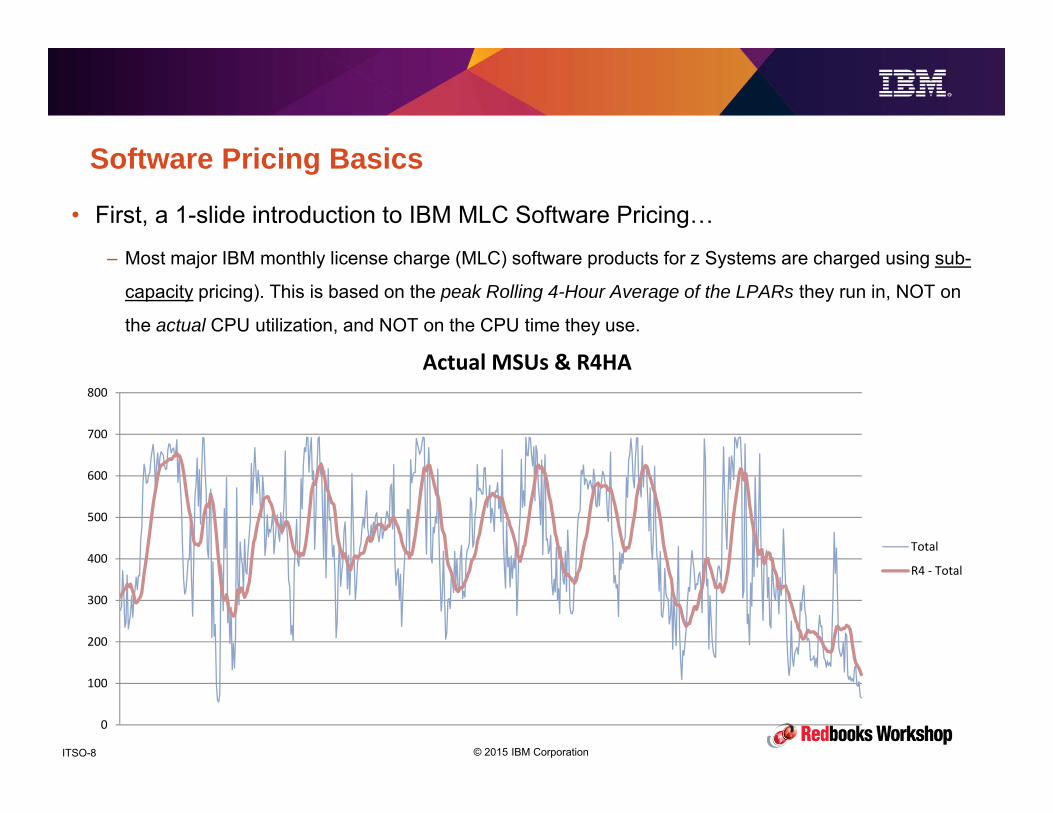
Software Pricing Basics
• First, a 1-slide introduction to IBM MLC Software Pricing…
– Most major IBM monthly license charge (MLC) software products for z Systems are charged using sub-
capacity pricing). This is based on the peak Rolling 4-Hour Average of the LPARs they run in, NOT on
the actual CPU utilization, and NOT on the CPU time they use.
0
100
200
300
400
500
600
700
800
Actual MSUs & R4HA
Total
R4 - Total

© 2015 IBM CorporationITSO-9
Software Pricing Basics
• Well, a 1(ish)-slide introduction to IBM MLC Software Pricing…
– To be precise, the charge is based on the lower of: the peak Rolling 4-Hour Average (R4HA – measured
in MSUs), or the highest defined capacity (specified in MSUs) for all the LPARs on that CPC running that
product for the month (00:00 on 2nd to 23:59 on the 1st)
– Remember that if you do something to lower the peak, some other interval becomes the new
peak and might be unaffected by the change you made.
0
100
200
300
400
500
600
700
800
900
1000
MSU
s
Time
R4HA
z/OS MSUs
Adjusted z/OS MSUs
00 23

© 2015 IBM CorporationITSO-10
Software Pricing Basics
• 1-slide introduction to IBM MLC Software Pricing (cont)…
– There is a bulk discount – the more MSUs you consume, the lower is the price per additional MSU.
– The AVERAGE cost per MSU is the total cost / peak R4HA.
– The INCREMENTAL cost per MSU is always less than the average and is the price you
pay for the next MSU.
0
50000
100000
150000
200000
250000
Mon
thly
Cos
t
MSUs
Pricing Curve
1372.35
386.4316.05
226.8120.75 92.4 65.1 49.35 39.9
0200400600800
1000120014001600
$ per Additional MSU

© 2015 IBM CorporationITSO-11
Software Pricing Basics
• 1-slide introduction to Software Pricing
(continued)…
– Basic rule is that each CPC is looked at in isolation
to determine your incremental $ per MSU.
– Assume you have 3 CPCs, all running
monoplexes, peak R4HA in each CPC is 315
MSUs:
– 3 x 93,184 = $279,555/Mth.
– But, if 1 sysplex accounts for > 50% of used MVS
MIPS on multiple CPCs, software is priced based on
aggregated MSUs across those CPCs.
– If the 3 CPCs qualified for sysplex aggregation,
the total MSUs would be 945, and the cost would
be: 1 x 156,949/Mth.
– This group of CPCs is called a PricePlex
0
50000
100000
150000
200000
250000
Mon
thly
Cos
t
MSUs
Pricing Curve
x3
© 2015 IBM CorporationITSO-12
Software Pricing Basics
• 1-slide introduction to Software Pricing (I TOLD you this wasn’t simple….)….
– Sysplex aggregation determines the $ per MSU you pay – where you are on the pricing curve.
– But the IBM software bill for each MLC product is based on the sum of the peak Rolling 4-hour
Averages for each LPAR that that product is used in for each CPC.
– So the highest interval for CPC1 is used, plus the highest interval for CPC2 (which is probably at
a different time), plus the highest interval for CPC3 (which is also probably at a different time).
– QUESTION for you to think about – how would your software bill be affected if you moved a major
workload:
– From one LPAR to another on the same CPC?
– From one LPAR to an LPAR on a different CPC?
© 2015 IBM CorporationITSO-13
Why techies need to know SW pricing
• Traditionally, software contract staff worked with vendors and decided on which
software pricing metric to use, often working independently of mainframe
technical staff.
• And mainframe technical staff aimed to deliver the best performance from the
available capacity, often without understanding or thinking much about software
pricing metrics.
– Generally, the same pricing metric (PSLC, VWLC, AWLC, etc) was used for every LPAR on a CPC
and for every CPC in the installation, so you didn’t really need to be aware of the pricing metric
when deciding what to put where.
– There are (OF COURSE) a small number of exceptions like zNALC (for ‘new’ applications) or
MULC (measured usage, for very small usage of some products in large LPARs), but these are
not very widely used.

© 2015 IBM CorporationITSO-14
Why techies need to know SW pricing
• Between z900 and z10, IBM provided a financial incentive (‘technology
dividend’) to move to newer CPCs by increasing the number of MIPS per
Software MSU with each generation. Or, to put it another way, the number of
MSUs required to process a given amount of work DEcreased. Software MSUs
are the base for most software pricing, so this let you do the same amount of
work for less money. THIS WAS GOODNESS!
0
200
400
600
800
1000
1200
z900 z990 z9 z10 z196
MSUs needed to do same amount of work
MSUs

© 2015 IBM CorporationITSO-15
Why techies need to know SW pricing
• The downside was that capacity management became more complex. An
LPAR on a z10 with a 1000 MSU cap could process more work than an LPAR
on a z9 with the same (1000 MSU) cap.
• This complicated the process of managing LPAR sizes and routing work to the
‘best’ system.
0
1000
2000
3000
4000
5000
6000
7000
8000
9000
z900 z990 z9 z10 z196
MIPS for 1000 MSUs
MIPS

© 2015 IBM CorporationITSO-16
Why techies need to know SW pricing
• An aside….. When is an MSU not an MSU?
• The original idea of MSUs was as an indicator of CPC capacity.
– The MSU for a CPC was:
– The SU/Sec for that box x number of engines x 3600 (to get MSU/hr)./1,000,000
• When IBM started altering the number of MIPS in an MSU as a way of
discounting software, you now had TWO MSUs:
– “Hardware” MSU – calculated using the original formula – this is the basis for reporting in RMF Type
72 records & Workload Activity Reports and service units reporting in Type 30 records.
– “Software” MSU – used as the basis for software charging and is used in the RMF Type 70 records
& CPU Activity reports….

© 2015 IBM CorporationITSO-17
Why techies need to know SW pricing
• And what is a MIPS (Millions of Instructions Per Second)?
• In theory, MIPS is an indication of the speed of the processor….
• However can imagine that the MIPS for a processor depends on how long the
instructions take to complete.
– Some instructions take a LOT longer to complete than others – for example, moving characters from one
location in memory to another takes MUCH longer than adding the numbers in two registers.
• As a result, the ‘MIPS’ for a processor is very workload dependent – there is no
single MIPS number for any box and no tool that reports MIPS numbers. The typical
range between high and low is about 34%. So you need to be very careful any time
you use MIPS, ESPECIALLY in contracts…. We’ll come back to this again later…
• Now, to return to our originally scheduled program….. MSUs and z196….

© 2015 IBM CorporationITSO-18
Why techies need to know SW pricing• On z196, IBM stopped increasing the number of MIPS per MSU and instead used a
new pricing option called AWLC (or AEWLC) that charged a lower price per MSU than the predecessor pricing option (VWLC) to incent customers to move to z196.
• Starting with zEC12, discounts are applied during the IBM billing process, so that the price per MSU on a zEC12 (or z13) is lower than on a z196, but the number of MIPS per MSU was the roughly same on zEC12 (or z13) as on a z196.
• The financial effect is similar (you pay less per MIPS on newer CPCs), however the capacity management complexity is somewhat simplified.
010002000300040005000600070008000
z196 zEC12 z13
MIPS for 1000 MSUs
MIPS
© 2015 IBM CorporationITSO-19
Why techies need to know SW pricing
• Despite all the complexity of software contracts, one thing that has been
consistent up until now is the average price per MSU for a given LPAR on a
given CPC – 1000 MSUs costs xxxx dollars regardless of the mix of work
running in the LPAR… 1000 MSUs is 1000 MSUs.
• But the world is changing. Workloads are changing. IBM is incenting
customers to put new and more workloads on z/OS by reducing the cost per
MSU for certain workloads (this is GOOD). It is also making it possible to mix
new and traditional workloads in the same LPAR while still getting a discount for
the new workloads – this provides far more flexibility for how you configure your
systems. However this also means that the days of consistent $ per MSU for an
LPAR are over (this is …… EXCITING!).

© 2015 IBM CorporationITSO-20
Recent IBM MLC SW Pricing Options
• The three most recent pricing options are:
– Mobile Workload Pricing, announced in May 2014.
– z Systems Collocated Application Pricing, announced in April 2015
– Country Multiplex Pricing, announced in July 2015
• Lets look at each of these and see how they will impact YOU.
© 2015 IBM CorporationITSO-21
Mobile Workload Pricing• What is Mobile Workload Pricing (MWP)?
• Headline is that it offers a 60% discount on MSUs consumed by
CICS/DB2/IMS/MQ/WAS transactions that originated on a mobile device.
• 60 …. PERCENT …. OFF! WOW! What else is there to say??
• Quite a bit….

© 2015 IBM CorporationITSO-22
Introduction to MWP• First, mobile is not a fad, it is not going away.
– There are already large z/OS customers where mobile consumes up to 50% of their
z/OS capacity.
– Some banks are incenting customers to interact with them using mobile apps rather
than PCs, partly so that they can benefit from MWP.
– And these are only the early days – we are still in the 3277 phase…
• IBM (and many others) believe mobile use will out-accelerate all other
platforms over the next few years, so MWP is IBM’s attempt to capture
the mobile workloads that exploit existing z/OS applications, rather than
having customers host these applications on other platforms.– Important to note that MWP is aimed at customers that are re-using existing
z/OS applications with mobile platforms.

© 2015 IBM CorporationITSO-23
Introduction to MWP• MWP IS a REALLY significant offering from IBM - it indicates that IBM
acknowledges that it must improve the cost-competitiveness of z/OS if
customers are to grow and roll out new applications on this platform.– zCAP and CMP (both previewed with the z13 announcement) continue this trend.
• The latest pricing options are all aimed at reducing the cost of GROWTH. – They might not immediately reduce your SW bills, BUT, IF you grow your z/OS workloads
and exploit the new pricing options, at some point the bulk of your work will be priced at
the new, more competitive price points, and your traditional (higher-priced) work will be a
decreasing portion of the total work (and cost).
© 2015 IBM CorporationITSO-24
Introduction to MWP• If you sign up for Mobile Workload Pricing (it is optional, and you must
sign an agreement and supplements if you want to use it), IBM will reduce the R4HA FOR EVERY IBM MLC PRODUCT IN THAT LPAR in each interval by 60% of the corresponding R4HA of the MSUs consumed by CICS, DB2, IMS, MQ, or WAS transactions that originated from a mobile device.
• Important point here is that it is not only the subsystem where the transaction ran (CICS, for example) that is discounted. It is EVERY subcapacity IBM MLC product in that LPAR – SDSF, DB2, PL/1, you name it.
© 2015 IBM CorporationITSO-25
Introduction to MWP• Initial questions from techies after they hear about MWP are
normally:– Precisely what qualifies as a ‘mobile device’?
– How do you get the CPU time used by those applications so you can input it to MWRT (MWRT is PC-based version of SCRT if you use MWP)?
• But maybe your initial questions should be:– How much mobile do I have now – using MWP generates additional work
(for you and for the system), so would the savings justify the work? Or should we concentrate on getting better prepared now, and sign up later?
– Mobile users are usually customers that expect instant responses, so how do I give them the capacity they need, while also controlling my costs?
– How do I manage my budgets/capacity when one (constantly varying) part of my workload has a different price per MSU than the rest of my workload?
– EXACTLY how does MWP impact my bills?

© 2015 IBM CorporationITSO-26
Understanding MWP• ‘Success’ is all about expectation setting….
• If you promise this……………………...
• And deliver this…....
– You are a hero
• If you promise this……………………..
• And deliver this…..,
– You get to experience a ‘career transitioning event’

© 2015 IBM CorporationITSO-27
Understanding MWP• To ensure that MWP is perceived as a successful project, it is
vital that you control the expectations because the MWP message is already being mis-interpreted.….
– MWP is aimed at reducing the cost of growing z/OS workloads. It MIGHT reduce your current costs, depending on how much of your work is MWP-eligible and whether that coincides with your peak Rolling 4-Hour Average (R4HA).
– But the real intent is to let you add mobile workloads to z/OS at a much lower cost than was the case previously. So MWP is more about reducing the cost of adding workloads to z/OS than reducing your SW bill today.
– Let’s look at an example….

© 2015 IBM CorporationITSO-28
Understanding MWP
0
100
200
300
400
500
600
700
800
900
1000
MSU
s
Time
Impact of MWP on R4HA
z/OS MSUs
MWP MSUs
Adjusted z/OS MSUs

© 2015 IBM CorporationITSO-29
Understanding MWP• The first expectation (misunderstanding) that you must control: ‘signing up for MWP will
reduce my SW bill by 60%’. It might reduce your bill, but it WILL NOT reduce it by 60%.
• If you reduce the total number of MSUs on your bill by some amount, you are reducing them at the incremental cost, not the average cost so your bill will not decrease by the same percent as your MSUs
• Let’s say you have a 2400 MSU system and you did not sign up for MWP – the bill would be $230,123 (an average of $95.88 per MSU).
• Now assume that 1680 of the 2400 MSUs were MWP-eligible and that you DID sign up for MWP. The MWP discount would be roughly 1000 MSUs (60% of 1680). So (absolute best case) that would bring your bill back to 1400 MSUs – $185,138. That’s a reduction of nearly 20%, which should be great. But it is not 60%.
OR ?
1372.35
386.4 316.05 226.8120.75 92.4 65.1 49.35 39.9
0
500
1000
1500
$ per Additional MSU

© 2015 IBM CorporationITSO-30
Understanding MWPAnd, in reality, your peak R4HA will now be some other interval, so you are VERY unlikely to actually see your peak R4HA reduce by 1000 MSUs. But let’s look at a growth scenario instead.
Let’s say that you ADDED 1680 MSUs of mobile workload to the peak rolling 4 hour interval on your 2400-MSU system, but did NOT sign that system up for MWP pricing….. The average $ per MSU for the 2400 MSUs was $95.88. Because of the SW price curve, the additional 1680 MSUs would have cost an extra $67,037. An average of just $39.90 per MSU for those extra MSUs.
But if you DID sign that system up for MWP and met all the requirements, the additional cost for the 1680 MSUs of mobile work would have been $26,815 –$40,222 less than if you didn’t have MWP. By exploiting MWP, you grew the actual used MSUs by 70% but your bill only increased by 11.6% - just $15.96 per MSU.
– Of course, this assumes that the additional capacity was only used by MWP-eligible workloads.
© 2015 IBM CorporationITSO-31
Understanding MWP• Expectation number 2 – ‘signing up for MWP will definitely reduce my
existing bill by something’.
• Actual: Signing up for MWP will reduce the R4HA for each hour in the month
by 60% of the MSUs used by MWP-eligible workloads.
• As we saw in the earlier chart, IF you run a lot of MWP-eligible work at the
time of your current peak R4HA, MWP will probably save you money.
• If your current peak R4HA is at a time when there is little or no MWP-eligible
work (during the batch window, for example), then MWP probably will not
reduce your current bill by much.
– BUT, it may allow you to add mobile workload at other times of the day at zero additional
cost, even if the peak total MSUs exceeds the batch shift peak.

© 2015 IBM CorporationITSO-32
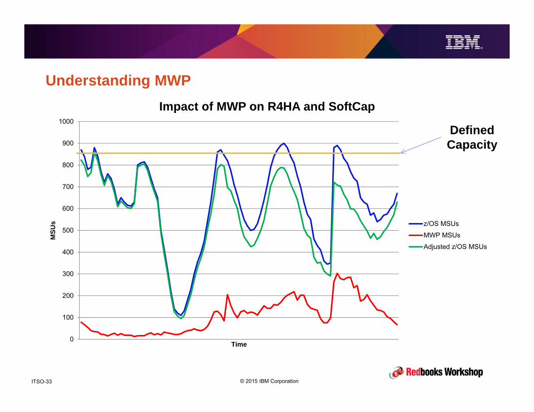
Understanding MWP• Expectation 3 – ‘MWP reduces the basis on which I get billed by 60% of the
capacity used by mobile’.
• Actual – MWP reduces the R4HA of every interval by 60% of the MSUs used by MWP-eligible work.
• You pay software bills based on the lower of: the peak R4HA for the month, or the highest defined capacity for the month.
• It is possible that the use of a defined capacity is already saving you most of what MWP would save you if you did not have a softcap.
• BUT, as the volume of your mobile work grows, the number of MSUs in that 60% discount will increase, so over time it will probably deliver more savings than a softcap alone.
• Let’s look at an example…..
© 2015 IBM CorporationITSO-33
Understanding MWP
0
100
200
300
400
500
600
700
800
900
1000
MSU
s
Time
Impact of MWP on R4HA and SoftCap
z/OS MSUs
MWP MSUs
Adjusted z/OS MSUs
Defined Capacity

© 2015 IBM CorporationITSO-34
Understanding MWP• To summarize the financial aspects of MWP:
• Given the global trend towards people being more reliant on their mobile devices, it is reasonable to expect that MWP WILL deliver real savings –some customers are already saving money with it.
• No one will reduce their IBM SW bill by 60% due to mobile.
– But real savings can be made and the cost of growth can be significantly reduced
– Just make sure that expectations are not set unrealistically high.
• If you don’t have much mobile work on your system today, don’t ignore MWP.
– This is good, because it gives you time to investigate and determine the best way for YOU to implement MWP and to work with subsystem sysprogs, application architects and developers, and contract administrators.
• Now let’s look at the technical considerations for how MWP affects your system and subsystem topology.
© 2015 IBM CorporationITSO-35
Managing an environment that has MWP• Part of the terms and conditions of MWP is that you must
have a way to identify the CPU time consumed by transactions that originated on a mobile device, and you are responsible for providing that information to MWRT (or a new version of SCRT). So everyone wants to know how to calculate the number of MSUs used by MWP-eligible work.

© 2015 IBM CorporationITSO-36
Managing an environment that has MWP• But before you break out your SMF and FORTRAN VS manuals, you
need to pause and consider something else: how do you control your SW costs in an MWP environment?
– Today, you can easily determine a reliable average and incremental cost per MSU for each of your LPARs based on the peak R4HA and product mix in each LPAR.
– Then you take your monthly SW budget and divide by the average cost per MSU amount, and that gives you your total Defined Capacity value.
– If your business requires predictable monthly bills, this is the most effective way to achieve that.
– But how do you do that when SOME (very variable) subset of your workload effectively has a different cost per MSU?
© 2015 IBM CorporationITSO-37
Managing an environment that has MWP
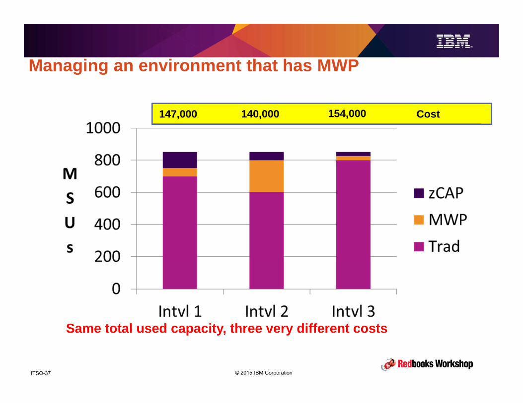
147,000 140,000 154,000 Cost
Same total used capacity, three very different costs

© 2015 IBM CorporationITSO-38
Managing an environment that has MWP• This is a very fundamental (and new) challenge for any site that is
interested in fully exploiting IBM’s recent software pricing options – your budgets are managed in dollars, but your LPARs are managed using MSUs, and the average price per MSU can constantly change depending on the workload mix.
• If you don’t add more capacity, you might not have sufficient capacity to deliver the required service level.
• But if you DO add more capacity, how much do you add? And how do you stop your traditional workloads from using all that capacity and increasing your costs beyond your budgeted amounts?
– You can use products to dynamically manage your defined capacities, but they also operate based on MSUs, so you still have the same challenge.
© 2015 IBM CorporationITSO-39
Managing an environment that has MWP• Ideally, you would be able to:
– Identify, in near-real time, how many MSUs are being used by each pricing option.
– Have a tool that would use that information to dynamically set and manage a defined capacity that would maximize the number of available MSUs, but without exceeding your financial targets.
• Today, the cost of gathering that information in real time at a transaction level might be higher than the savings that MWP would provide.
– Recently previewed WLM APAR OA47042 (z/OS 2.1 and later), combined with support in CICS and IMS, may provide relief IF the WLM classification criteria can be used to identify all MWP-eligible transactions. APAR is still open, due for delivery in December, and all details are not available yet. But if you are interested in MWP, this is an APAR to follow.
– Also, have a look at MXG 33.216 which already has the definitions for the new fields!
• With that in mind, let’s look at your options for how you could provide an environment for your MWP workloads.

© 2015 IBM CorporationITSO-40
Managing an environment that has MWP• You basically have 3 options:
– Run your MWP-eligible transactions in the same regions and subsystems as your traditional workloads.
– Provide regions and subsystems that are dedicated to MWP-eligible transactions, but that run in shared LPARs.
– Provide dedicated LPARs for the MWP-eligible transactions.
• Let’s look at the benefits and drawbacks of each of these.

© 2015 IBM CorporationITSO-41
Managing an environment that has MWP• Shared regions
• Benefits:
–EASY to set up – just use existing regions and subsystems.
• Drawbacks:– Currently, you MUST process
transaction-level SMF data to identify CPU consumption of MWP-eligible transactions. This could be a LOT of data.
– Identifying the source of the transaction from the SMF records might not be possible.
– How do you identify the original source of transactions that are called by other txns?
– Maintenance effort for programs that extract CPU usage info is not insignificant – every time a new MWP-eligible application is deployed or modified, you need to update your programs. And not every application will use the same mechanism for identifying its source.
• Drawbacks:– Transaction-level SMF records do not
capture region management time –about 80% is captured, at best.
– MQ does not provide transaction-level CPU usage info in its SMF records, so you are limited to collecting whatever MQ charges back to CICS/IMS/etc.
– Categorizing CPU usage in real time is currently expensive, maybe impossible (but OA47042 might help).

© 2015 IBM CorporationITSO-42
Managing an environment that has MWP• Dedicated regions in shared LPARs
• Benefits:– Might be easier to identify the
transaction source in the network and route it to the dedicated regions – removes the need to identify this from transaction-level SMF records.
– Because identification is done based on mobile device name, maintenance effort should be a lot lower than if you are gathering this info from transaction-level SMF or log records.
• Drawbacks:– Requires additional regions/subsystems,
meaning more work to set up and manage, plus the resources required for more address spaces.
– Requires data sharing if you want to extend this to database manager.
• Benefits:– IBM will accept data extracted
from SMF Type 30 records –massive reduction in volume of SMF data to be processed.
– Because Type 30 records are used, you capture all the management time as well.
– Possible to economically identify CPU consumption of these regions in real time, even without the WLM MWP support.

© 2015 IBM CorporationITSO-43
Managing an environment that has MWP• Dedicated systems• Benefits:
– All of the benefits of dedicated regions, plus….
– Dramatically easier to manage LPAR capacity, because nearly all work in the LPAR has the same average price per MSU.
– Easier to provide dedicated capacity for MWP work and have less important traditional work subject to capping in other LPARs.
– IBM will accept data from just the Type 70 and Type 89 records – no need to collect, keep, and post-process transaction-level or even address space-level SMF records.
• Drawbacks:
– Setting up new systems means more work to set up and manage, plus the resources required for more LPARs.
– Requires data sharing, assuming that you want to share data between MWP and traditional applications.
• Benefits:– There might be security advantages
to isolating transactions originating on a mobile device into their own LPARs.

© 2015 IBM CorporationITSO-44
Implementing MWP• Regardless of which topology you decide to use, you are responsible for
getting CPU usage data into a format that can be used by MWRT.
• IBM currently do not provide any mainstream tool to do this processing.
– They do have a product called Transaction Analysis Workbench 1.2 (5697-P37) that purportedly helps you gather data for MWP if APAR PI29291 is applied, but I have not been able to get any more information about this.
– In time, the WLM MWP support might collect all the data you need in the Type 72 and Type 99 SMF records, however you will still be responsible for getting it from there into a format that can be input to MWRT/SCRT.
• Al Sherkow and Barry Merrill have produced some tools based on MXG.
– But they are still limited by the information that can be found in the SMF records.
– MXG already supports the new WLM MWP support, which might or might not identify all mobile transactions.
– And they still require customer programming.

© 2015 IBM CorporationITSO-45
Implementing MWP• In order to be able to avail of MWP, you must:
– Have a zBC12 or zEC12 or later in your enterprise.
– The MWP-eligible workloads must run on a z114/z196 or later.
– Be running z/OS (V1 or V2) and one or more of CICS (V4 or V5), DB2 (V9, V10, or V11), IMS (V11, V12, or V13), MQ (V7 or V8), or WAS (V7 or V8).
– Be using a sub-capacity pricing option – AWLC, AEWLC, or zNALC.
– Sign the MWP supplement.
– And agree with IBM which applications will be eligible, and how you will gather the usage data for those applications. And, especially, exactly how you will identify the MWP-eligible transactions.
– Also, any time you add new MWP transactions/applications, you must inform IBM and complete a new supplement.
– Provide your own mechanism to create the MWP input to MWRT (or SCRT 23.10 or later).
– Use MWRT or SCRT 23.10 or later to report your utilization to IBM.

© 2015 IBM CorporationITSO-46
MWP Summary• Investigate if MWP would help you today, and to what extent.
• Set management’s expectations to a realistic level and position this as a strategic direction to reduce future costs.
• Work with subsystem sysprogs, application developers, whoever owns the WLM policy, and contract administrators to identify the most efficient topology for your company, bearing in mind zCAP and other similar options that may follow.
– And don’t forget that you need some way to ensure that the additional capacity you provide for MWP work is not used by traditional work.
• Work with subsystem sysprogs and application developers to investigate how you can identify MWP-eligible transactions – if possible, use consistent mechanism to simplify programs that extract MWP CPU time info.
• Create and test programs to extract the required data into MWR-readable format.
• Sign the IBM agreements and supplements.
• Plan for what you will spend your MASSIVE bonus on….
© 2015 IBM CorporationITSO-47
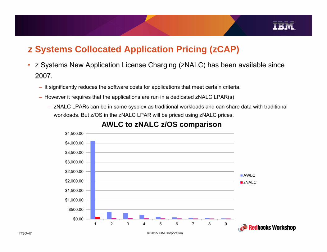
z Systems Collocated Application Pricing (zCAP)• z Systems New Application License Charging (zNALC) has been available since
2007.– It significantly reduces the software costs for applications that meet certain criteria.
– However it requires that the applications are run in a dedicated zNALC LPAR(s)
– zNALC LPARs can be in same sysplex as traditional workloads and can share data with traditional workloads. But z/OS in the zNALC LPAR will be priced using zNALC prices.
$0.00
$500.00
$1,000.00
$1,500.00
$2,000.00
$2,500.00
$3,000.00
$3,500.00
$4,000.00
$4,500.00
1 2 3 4 5 6 7 8 9
AWLC to zNALC z/OS comparison
AWLC
zNALC
© 2015 IBM CorporationITSO-48
z Systems Collocated Application Pricing
• To address the needs of customers that have new applications but that don’t
want to have to set up dedicated LPARs for those workloads, IBM introduced a
new pricing option called z Systems Collocated Application Pricing (zCAP).
• zCAP is conceptually similar to MWP in that discounts are based on the
middleware CPU consumption of applications that meet the criteria for zCAP
and that are described in your zCAP agreement and supplements with IBM.
• However, because the applications are NEW, they should be a lot easier to
identify than MWP transactions, which use existing applications (meaning that
you don’t have the complexity of trying to determine the source of the
transaction).

© 2015 IBM CorporationITSO-49
z Systems Collocated Application Pricing• What is a ‘new’ workload?
– Must be a new application to z/OS in your enterprise.
– Does not have to be new ‘in the universe’ – for example, SAP has been around for many years, but if you are not using SAP on z/OS now, then it is eligible to be considered ‘new’ for zCAP purposes.
– If you move SAP from another platform in your enterprise to z/OS, that also counts as being ‘new’ for zCAP purposes.
– The zCAP definition of ‘new’ is a lot more flexible than the zNALC definition of new. Application must use at least one of CICS/DB/IMS/MQ/WAS, but that is all.
• The objective is to provide you with more flexibility to help you add new z/OS applications.
• Organic growth of existing applications does not count as ‘new’ for zCAP purposes.• For gray areas, speak to IBM and make a case for why the application should be
considered ‘new’.• Also, in the words of IBM’s David Chase, ‘newness does not wear off. Applications
that qualified as ‘new’ 5 years ago are still considered new today’.

© 2015 IBM CorporationITSO-50
z Systems Collocated Application Pricing
• Like MWP, you have to identify the MSUs used by the zCAP-eligible workload
(CICS/DB2/IMS/MQ/WAS).
– Then you subtract 50% of that amount from the z/OS R4HA.
– And you subtract 100% of that amount from all other MLC products in the LPAR (CICS, DB2, IMS,
MQ, WAS, COBOL, NetView, etc.)
– Then you pay for the MSUs for the subsystems used by the zCAP-eligible workload using the same
pricing metric that is being used by the LPAR the application is running in.
• Let’s look at two scenarios….
– First one is where a new application is the only user of a ‘zCAP-defining’ subsystem
(CICS/DB2/IMS/MQ/WAS)
– Second one is where the new application uses an existing subsystem.

© 2015 IBM CorporationITSO-51
z Systems Collocated Application PricingNet New MQ Example = 100 MSUs of new MQ workload *
1. Existing LPAR 2. New MQ, standard rules 3. New MQ with zCAP pricing
MSUs used for subcap billing: MSUs used for subcap billing: MSUs used for subcap billing:z/OS 1,000 z/OS 1,100 z/OS 1,050DB2 and CICS 1,000 DB2 and CICS 1,100 DB2 and CICS 1,000
MQ (LPAR value) 1,100 MQ (usage value) 100
Standard LPAR Value = 1,100 Standard LPAR Value = 1,100z/OS, other programs adjusted
Standard LPAR Value = 1,0001,100 1,100 1,100
1,0501,000 1,000 1,000
z/OS DB2 z/OS DB2 MQ z/OS DB2& CICS & CICS & CICS
MQ100
* Assumes workloads peak at same timeExample courtesy of David Chase, IBM
© 2015 IBM CorporationITSO-52
z Systems Collocated Application Pricing
• Consider what would have happened if you had used zNALC for this
application…
– You would have paid a discounted price for z/OS based on a 100 MSU R4HA.
– You would have paid for 100 MSUs of MQ
• Because you are using zCAP in this example:
– The MSU value used for CICS & DB2 was reduced by 100% of the capacity used by the new
application because it didn’t use either of those products – so you paid for 1000 MSU of CICS or
DB2, rather than 1100 MSUs.
– You reduced the total z/OS R4HA number by 50% of the capacity used by the new application (50
MSU reduction) so you paid for 1050 MSUs of z/OS.
– You only paid for 100 MSUs of MQ, even though it lived in an LPAR that was using 1100 MSUs.
• So the net effect may be similar to zNALC, but without the need for a separate
LPAR.

© 2015 IBM CorporationITSO-53
z Systems Collocated Application PricingIncremental MQ Example = 100 MSUs of MQ growth *
1. Existing LPAR 2. MQ growth, standard rules 3. MQ growth with zCAP pricing
MSUs used for subcap billing: MSUs used for subcap billing: MSUs used for subcap billing:z/OS 1,000 z/OS 1,100 z/OS 1,050DB2 and CICS 1,000 DB2 and CICS 1,100 DB2 and CICS 1,000MQ 1,000 MQ w/growth 1,100 MQ w/growth 1,100
Standard LPAR Value = 1,100 Standard LPAR Value = 1,100z/OS, other programs adjusted
Standard LPAR Value = 1,000 1,100 1,1001,100 1,100 100 of 100 of
growth 1,050 growth1,000 1,000 1,000 1,000
z/OS DB2 MQ z/OS DB2 MQ z/OS DB2 MQ& CICS & CICS & CICS
* Assumes workloads peak at same timeExample courtesy of David Chase, IBM

© 2015 IBM CorporationITSO-54
z Systems Collocated Application Pricing• In this example, the new application used a product (MQ) that was already being
used by existing applications:– The MQ cost went up by the 100 MSUs that the application was using.
– The R4HA value used for CICS & DB2 was reduced by 100 because the new application didn’t use CICS
or DB2.
– The total z/OS MSU number was reduced by 50% of the capacity used by the new application (50 MSU
reduction).
– The R4HA for every other MLC product would be reduced by the 100 MSUs.
• So, again, the net effect is similar to zNALC, but without the need for a separate
LPAR.– With zNALC you would pay for 100 MSUs of z/OS at the very-reduced zNALC rate. With zCAP, you would
pay for 50 MSUs of z/OS at your incremental price for z/OS (with the price depending on where you are on
the pricing curve for z/OS).
– The relative costs of MQ would depend on if you use AWLC or Value Unit Edition (IPLA, only available
with zNALC) and where you are on the pricing curve.

© 2015 IBM CorporationITSO-55
z Systems Collocated Application Pricing
• As with MWP, you are responsible for identifying the capacity used by the new
workload and translating that into a CSV file that is input to MWRT (or new
SCRT).
– If the new application is the only user of a subsystem (as in the 1st example), it is acceptable to use
data from the Type 89 SMF records.
– If the application is using an existing subsystem product (MQ, in example 2), but runs in its own
dedicated region, IBM will accept data from the Type 30 records for that region.
– If the application is using an existing subsystem AND an existing region, then you need to use
transaction-level information to determine the MSUs used by the new application.

© 2015 IBM CorporationITSO-56
z Systems Collocated Application Pricing Requirements
• zCAP is only available for new applications that run in a z114/z196 or later with
AWLC, AEWLC, CMLC, or zNALC sub-capacity pricing.
• Supports both z/OS V1 and V2, and current and recent versions of
CICS/DB2/IMS/MQ/WAS.
• Data must be submitted to IBM using MWRT 3.3.0 or later (current version is
3.3.5) or SCRT 23.10 or later.
• There is a new contract Addendum and accompanying Supplement:
– Addendum for z Systems Collocated Application Pricing (Z126-6861)
– Terms and conditions to receive zCAP benefit for AWLC, AEWLC, zNALC billing
• Supplement to the Addendum for zCAP (Z126-6862)
– Customer explains how they measure their zCAP application CPU time
– Agreement to and compliance with the terms and conditions specified in the zCAP contract
Addendum is required

© 2015 IBM CorporationITSO-57
z Systems Collocated Application Pricing Summary
• zCAP has a similar objective to zNALC – reduce the cost of adding ‘new’
applications to z/OS.
• But it is intended to give you an alternative to running dedicated zNALC LPARs
– you can now select a topology that makes both financial and technical sense.
• It is not possible to make a blanket statement about which option (zNALC or
zCAP) will have lower costs. Recommend that you work with your IBMer to price
the following options:
– Straight AWLC/AEWLC.
– zCAP.
– zNALC with AWLC/AEWLC for subsystems.
– zNALC with IPLA for subsystems.
– Don’t forget to factor in cost of dedicated LPAR for zNALC.

© 2015 IBM CorporationITSO-58
Country Multiplex Pricing
• The most recent pricing option is Country Multiplex Pricing (CMP), announced in
July 2015.
• Its primary objective is to address customer issues with sysplex aggregation and
provide customers with much more flexibility regarding how you configure your
systems and sysplexes – it aims to eliminate financial incentives to create
configurations that make no technical sense.
• For any customer that has or would like to have a sysplex,
this is THE BEST THING EVER!
• Let’s look at some of the issues that it addresses. And then we will look at some
scenarios to see how it would affect your SW bills.
© 2015 IBM CorporationITSO-59
Country Multiplex Pricing
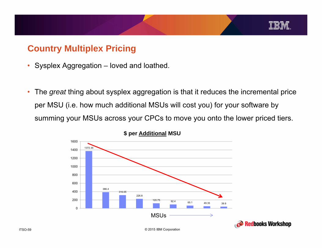
• Sysplex Aggregation – loved and loathed.
• The great thing about sysplex aggregation is that it reduces the incremental price
per MSU (i.e. how much additional MSUs will cost you) for your software by
summing your MSUs across your CPCs to move you onto the lower priced tiers.
1372.35
386.4316.05
226.8
120.75 92.4 65.1 49.35 39.9
0
200
400
600
800
1000
1200
1400
1600
$ per Additional MSU
MSUs

© 2015 IBM CorporationITSO-60
Country Multiplex Pricing• The not-so-great thing is that your business structure might not be consistent with
creating a sysplex that accounts for >50% of all used MVS MIPS.– Companies have production systems, development systems, test systems, quality assurance systems, and
sysprog systems – they each have a specific purpose and objectives that might clash with each other.
– Your business might consist of multiple companies that do not share data or applications, so there is no logical reason for them to be in the same sysplex.
• But to get over the magical 50% sysplex aggregation threshold, some customers create sysplexes that are sysplexes in name only.
– Mixing test and production.
– Mixing completely unrelated systems in the same sysplex.
– Only criteria is the number of MSUs used by the system, not its relationship to other systems in the sysplex.
• Valuable and scarce technical resource is expended on creating and maintaining an environment that delivers zero business advantage to the enterprise. It would be far more valuable to use those skills to implement new business functions and products.

© 2015 IBM CorporationITSO-61
Country Multiplex Pricing
• If you switch to Country Multiplex Pricing, the R4HA for every LPAR across
every CPC in a country is used to determine your incremental software cost,
regardless of whether the systems are in the same sysplex (or ANY sysplex) or
not.
• No more financial encouragement to create shamplexes (as long as you
are already using CMP) – YIPEE!

© 2015 IBM CorporationITSO-62
Country Multiplex Pricing
• Mixing different types of system (test and production, for example) in the same
sysplex can cause system and sysplex outages.
– This is why IBM’s best practice guidelines say not to mix test and production in the same sysplex.
– Test systems are used for ….. Testing. It is the nature of those systems to have new, untested
software. Compare that to production, which requires stability, control, consistency, manageability
• Despite the known problems, people still created such sysplexes because of the
short term financial savings.
• With CMP, there is no connection between the use of sysplex and your
software costs.
• So, after you move to CMP, there is ZERO incentive to ever create
nonsensical sysplexes again…. YIPEE (again)

© 2015 IBM CorporationITSO-63
Country Multiplex Pricing• For technical reasons, you might wish to keep production and non-production
systems on separate CPCs.– For example, you want to be able to test new HW functions in a safe environment before moving them to
production.
– Or you want to place a production CF on a CPC that doesn’t have any production z/OS systems. This config has the same failure-isolation characteristics as a standalone CF, but at a lower cost.
• But because of the financial benefit of sysplex aggregation, there was a very strong incentive to include as many CPCs as possible in the sysplex, making it very difficult to have a completely failure-isolated CPC.
• With CMP, the number of CPCs that a sysplex is spread across has zero impact on MLC prices. So you could have 2 production CPCs and 2 test CPCs, or 4 production/test CPCs – the MLC SW cost would be the same.
• Now you can really configure for the optimum configuration without being constrained by financial considerations.
© 2015 IBM CorporationITSO-64
Country Multiplex Pricing
• There are many factors that play into identifying the optimum physical location
of your CPCs:
– Availability and cost of data center space
– Disaster recovery considerations
– Location and condition of existing corporate data centers
– Availability of skills
– Infrastructure and natural hazards – earthquakes, flooding, ice storms, reliable power supply
– And, prior to CMP, sysplex distances (so you can include both data centers in sysplex aggregation)
• With CMP, because the sysplex aggregation requirement has gone away,
the location of your CPCs (as long as they are in the same country) has no
impact on your MLC software costs, so you are free to determine their
location based purely on business and technical considerations.
© 2015 IBM CorporationITSO-65
Country Multiplex Pricing
• Prior to CMP, when calculating your software bill for the month, IBM uses the sum
of the peak R4HAs for each CPC for the month.
• It is unlikely that all your CPCs will peak at exactly the same time. As a result,
your bill is probably based on more MSUs than you actually use at any one point
in time.

© 2015 IBM CorporationITSO-66
Country Multiplex PricingCPC1 CPC2 CPC3 CMLC SUM
LP1 LP2 LP3 LP4AWLCSUM LP1 LP2 LP3
AWLCSUM LP1 LP2
AWLCSUM
0:00 55 232 13 563 863 0:00 217 101 392 710 0:00 148 183 331 19041:00 64 481 49 246 840 1:00 276 392 384 1052 1:00 71 62 133 20252:00 60 454 15 255 784 2:00 235 382 65 682 2:00 179 288 467 19333:00 73 279 38 342 732 3:00 166 269 202 637 3:00 348 321 669 20384:00 75 257 37 671 1040 4:00 108 218 347 673 4:00 260 115 375 20885:00 52 442 32 329 855 5:00 369 86 122 577 5:00 450 123 573 20056:00 61 415 17 172 665 6:00 315 342 123 780 6:00 241 74 315 17607:00 75 406 12 168 661 7:00 366 293 155 814 7:00 148 340 488 19638:00 66 465 12 159 702 8:00 117 64 100 281 8:00 103 363 466 14499:00 68 374 18 390 850 9:00 154 264 347 765 9:00 446 155 601 2216
10:00 63 350 50 571 1034 10:00 266 83 220 569 10:00 229 399 628 223111:00 66 395 22 382 865 11:00 339 120 336 795 11:00 244 373 617 227712:00 52 459 24 263 798 12:00 342 247 318 907 12:00 304 211 515 222013:00 74 412 46 508 1040 13:00 233 239 132 604 13:00 140 207 347 199114:00 53 443 48 164 708 14:00 122 144 270 536 14:00 286 191 477 172115:00 63 296 26 691 1076 15:00 256 378 152 786 15:00 447 227 674 253616:00 60 342 21 178 601 16:00 86 335 176 597 16:00 315 348 663 186117:00 61 417 33 199 710 17:00 132 106 163 401 17:00 151 153 304 141518:00 72 495 9 535 1111 18:00 188 219 81 488 18:00 409 215 624 222319:00 73 304 22 460 859 19:00 185 160 384 729 19:00 210 445 655 224320:00 53 459 30 694 1236 20:00 321 361 149 831 20:00 269 306 575 264221:00 56 463 39 453 1011 21:00 198 370 67 635 21:00 158 115 273 191922:00 72 201 37 418 728 22:00 66 392 286 744 22:00 217 340 557 202923:00 58 283 17 602 960 23:00 243 133 154 530 23:00 257 269 526 20160:00 59 321 44 528 952 0:00 384 72 91 547 0:00 155 177 332 18311:00 53 471 46 406 976 1:00 54 344 373 771 1:00 224 203 427 2174
Peak 1236 1052 674 2962 2642

© 2015 IBM CorporationITSO-67
Country Multiplex Pricing
• With CMP, your peak R4HA is determined by summing every LPAR on every
CPC, effectively working as if every LPAR was in the one CPC.
• The result is likely to be a lower peak R4HA number than would be
calculated using pre-CMP rules.
© 2015 IBM CorporationITSO-68
Country Multiplex Pricing• Because your bill was based on the peak R4HA for the month for each CPC, if you moved an
application from one CPC to another, you would end up paying for the capacity used by that
application on BOTH CPCs for that month.
• For the same reason, some customers are unwilling to enable queue sharing or dynamic
workload routing (especially across two sites) because that could result in work moving between
CPCs more than would happen with static routing.
– But by not exploiting these technologies, you are losing a lot of the benefit of data sharing and probably getting
longer response times and less efficient resource usage than if you let WLM or shared queue manager control the
routing.
• Because CMP calculates your peak R4HA by summing every LPAR on every CPC, moving
work from one CPC to another should have no impact on your MLC software bill
• There is now no financial reason NOT to fully exploit the workload routing options that are available to you or to move workloads between CPCs.

© 2015 IBM CorporationITSO-69
Country Multiplex Pricing
• Single Version Charging (SVC) saves you money by letting you pay for two
versions of a product as if they were one version (GOOD). – Remember that you pay based on LPAR sizes, so if you didn’t have SVC, you would pay for both
versions based on the LPAR’s peak R4HA. With SVC you only pay for the latest version.
• However, you generally only have 1 year to complete the migration to the new
version (NOT SO GOOD).– COBOL V5 now offers 1.5 years for migration.
• CMP provides a feature known as Multiple Version Migration. With MVM, you
pay for all installed versions of a product as if they were the most recent version
(similar to SVC), however there is no limit on how long you take to migrate.
If you wish, you could run both versions indefinitely. You can even run more
than two versions.
© 2015 IBM CorporationITSO-70
Country Multiplex Pricing• Because your software bill is based on peak R4HA (or peak defined capacity) for
each CPC, increasing the defined capacity on one CPC would probably result in an increase in your software bill for that month even if you reduced the defined capacity on another CPC by a similar amount.
• Because CMP is based on the peak R4HA/peak defined capacity across all your CPCs, decreasing the defined capacity on one CPC would allow you to increase the defined capacity on another CPC without impacting your MLC software bill (just as moving a defined capacity from one LPAR to another on the same CPC today would not impact your software bill).
• This allows you to get the full benefit of installed capacity spread across multiple CPCs without your MLC SW bill going up. Ideal if you have different CPCs that service different time zones, or if you have affinities between workloads and specific LPARs.

© 2015 IBM CorporationITSO-71
Country Multiplex Pricing
• What’s the catch? CMP is primarily designed to increase flexibility, separate
financial considerations from technical decisions, and help improve availability –
these benefits are available to anyone that signs up for CMP. And it lets you
reconfigure into a more sensible sysplex topology (no longer spreading one
sysplex over every CPC, for example), without increasing your software costs.
• While it should also enable growth at reduced costs, that is not its primary
objective.– If your CPCs are not aggregated today, CMP should reduce the cost of adding capacity.
– If your CPCs ARE aggregated today, most of the CMP financial benefit will probably come above
2500 MSUs - up to 2500 MSUs, CMLC prices are the same as AWLC.
• In return for the greater flexibility that CMP provides, future bills are calculated
as a delta off your current bill.
• How does this work???
© 2015 IBM CorporationITSO-72
Country Multiplex Pricing• Prior to moving to CMP, IBM calculates 2 baselines for each product:
• One is based on the average of the peak R4HA across all your CPCs for the 3
months your last 3 bills are based on – this is called the MSU Base.– Note that this value is arrived at using the same methodology as CMP – the total R4HA for each interval is
calculated by summing the R4HA for every LPAR on every CPC.
– As a result, this value probably will be different to the values that were used to calculate your bill for those
3 months, but it is consistent with how your bill will be calculated after you move to CMP.
• The other baseline is the average of the billed amount ($s) for each of the prior 3
months – this is called the MLC Base.
• The % difference between the MLC base and what the price would have been,
based on the CMLC rules and tiers is calculated – this is called the MLC Base Factor.
• These values will all be documented in your CMLC agreement.
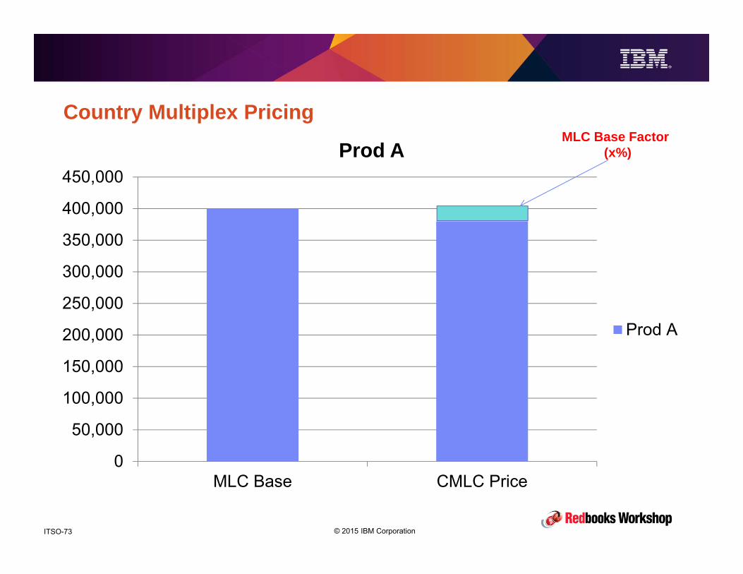
© 2015 IBM CorporationITSO-73
Country Multiplex Pricing
0
50,000
100,000
150,000
200,000
250,000
300,000
350,000
400,000
450,000
MLC Base CMLC Price
Prod A
Prod A
MLC Base Factor (x%)
© 2015 IBM CorporationITSO-74
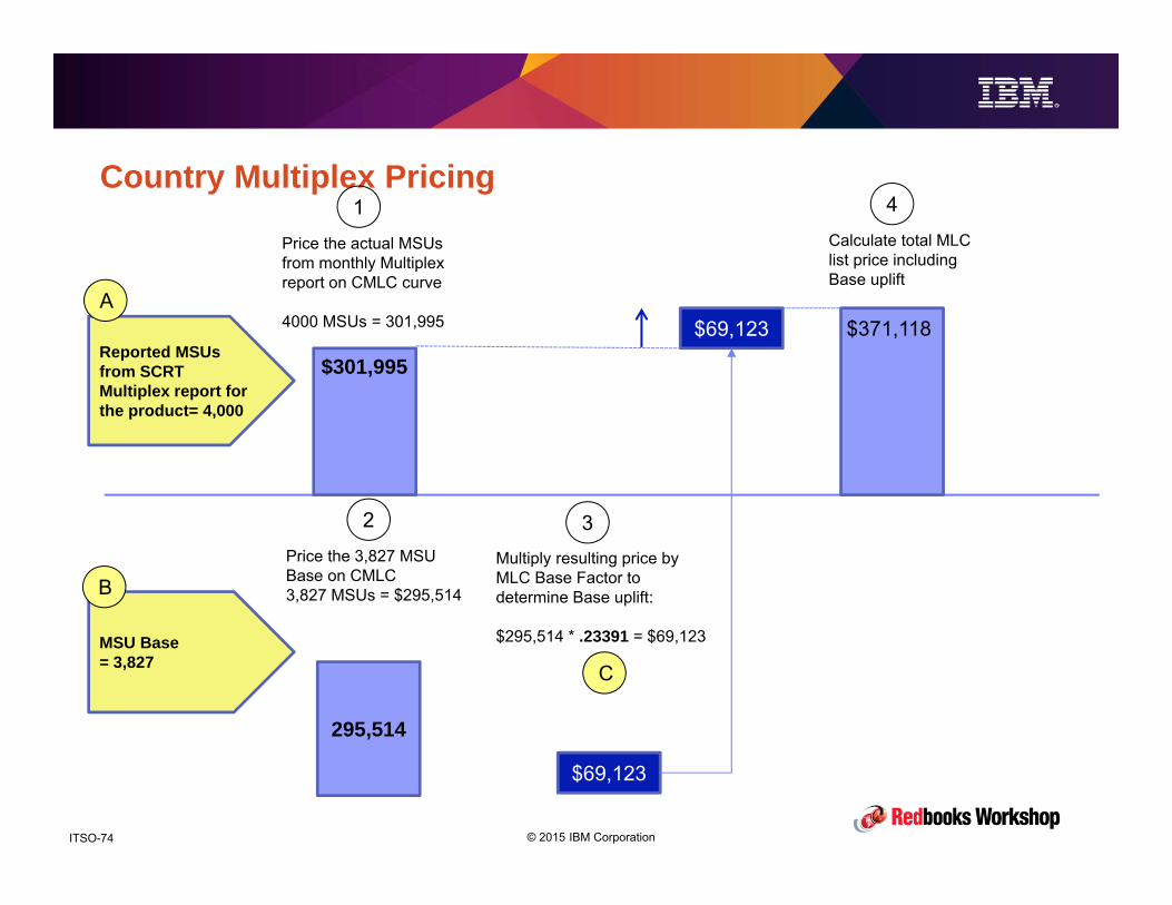
Country Multiplex Pricing
Reported MSUs from SCRT Multiplex report for the product= 4,000
$69,123
$301,995
$371,118
MSU Base= 3,827
Price the actual MSUs from monthly Multiplex report on CMLC curve
4000 MSUs = 301,995
295,514
Calculate total MLC list price including Base uplift
Price the 3,827 MSU Base on CMLC3,827 MSUs = $295,514
1
2 3
4
$69,123
Multiply resulting price by MLC Base Factor to determine Base uplift:
$295,514 * .23391 = $69,123
A
B
C

© 2015 IBM CorporationITSO-75
Country Multiplex Pricing
• After you move to CMP, your bill is calculated as follows:
1. The peak R4HA is used to calculate what the CMLC price would be.
2. Then the current CMLC price of the MSU Base is calculated.
3. Multiply the answer from 2 by the MLC Base Factor to get the MLC uplift
4. Add 3 to 1 to determine your actual CMLC bill
• Let’s look at some scenarios to see how this might affect YOU.
© 2015 IBM CorporationITSO-76
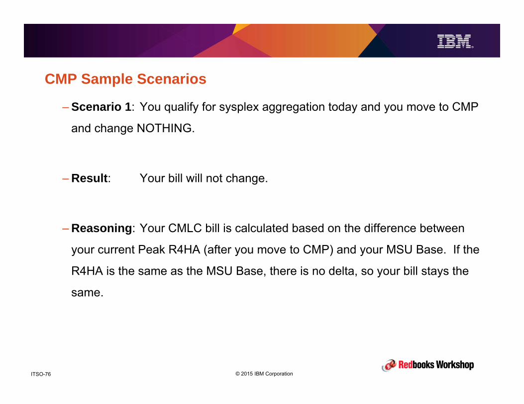
CMP Sample Scenarios
– Scenario 1: You qualify for sysplex aggregation today and you move to CMP
and change NOTHING.
– Result: Your bill will not change.
– Reasoning: Your CMLC bill is calculated based on the difference between
your current Peak R4HA (after you move to CMP) and your MSU Base. If the
R4HA is the same as the MSU Base, there is no delta, so your bill stays the
same.

© 2015 IBM CorporationITSO-77
CMP Sample Scenarios
– Scenario 2: You qualify for sysplex aggregation today then move to CMP
and break up shamplexes but everything else stays the same
– Result: Your bill will not change.
– Reasoning: Again, because your new R4HA is the same as the MSU Base,
there is no delta, so your bill stays the same.
– Note that if you had done this BEFORE you moved to CMP, your bill
would probably have increased dramatically.

© 2015 IBM CorporationITSO-78
CMP Sample Scenarios– Scenario 3: You do NOT qualify for sysplex aggregation today. Then you sign
up for CMP and don’t change anything.
– Result: Your bill will not change.
– Reasoning: Remember that the MSU Base is calculated by summing across all CPCs. The MLC Base depends on whether you were aggregated before, but the MSU Base does not. So, because your new R4HA is the same as the MSU Base, there is no delta, so your bill stays the same. Even though CMP does not require sysplex aggregation, the MLC Base at the time you move to CMP determines your future bills. So, it doesn’t matter if you stay aggregated AFTER you move to CMP, but you want to stay aggregated up until you make the move.
© 2015 IBM CorporationITSO-79
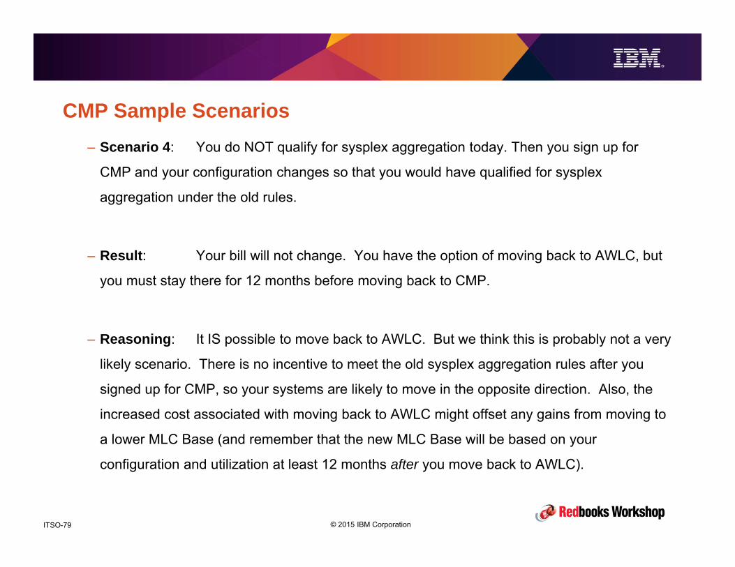
CMP Sample Scenarios– Scenario 4: You do NOT qualify for sysplex aggregation today. Then you sign up for
CMP and your configuration changes so that you would have qualified for sysplex
aggregation under the old rules.
– Result: Your bill will not change. You have the option of moving back to AWLC, but
you must stay there for 12 months before moving back to CMP.
– Reasoning: It IS possible to move back to AWLC. But we think this is probably not a very
likely scenario. There is no incentive to meet the old sysplex aggregation rules after you
signed up for CMP, so your systems are likely to move in the opposite direction. Also, the
increased cost associated with moving back to AWLC might offset any gains from moving to
a lower MLC Base (and remember that the new MLC Base will be based on your
configuration and utilization at least 12 months after you move back to AWLC).
© 2015 IBM CorporationITSO-80
CMP Sample Scenarios
– Scenario 5: You have 2 priceplexes today. You sign up for CMP. And grow
by 1000 MSUs.
– Result: Your bill will increase. The amount of the increase is likely to be
less than would have been the case if you had grown by the same amount
under AWLC.
– Reasoning: Each priceplex is likely to be on a steeper part of the pricing
curve. When all the processors are in CMP, the peak R4HA will be calculated
across all CPCs, very likely resulting in the incremental price per MSU being
lower because the configuration is on the flatter part of the pricing curve.

© 2015 IBM CorporationITSO-81
CMP Sample Scenarios– Scenario 6: You have 1 priceplex today. In the middle of the month you move a
workload from CPC1 to CPC2. Peak MSUs on CPC1 is 750 MSUs before the move,
and the peak R4HA on CPC2 is 750 after the move. Even though the combined peak
never exceeds 850 MSUs, the bill would be for 1500 MSUs based on the two peak
MSUs. Then you sign up for CMP and make the same move in reverse but everything
else remains the same.
– Result: Moving the application will not cause your bill to increase.
– Reasoning: Because the Peak R4HA is calculated based on the sum of all LPARs
across all CPCs, moving a workload from one CPC to another under CMP has the
same effect as moving a workload from one LPAR to another prior to CMP.

© 2015 IBM CorporationITSO-82
CMP Requirements
• Must be running z/OS V1 or later.
• If you sign up for CMP, ALL CPCs in your enterprise in the country that
run z/OS must be included.
• You can only sign up for CPC if ALL your z/OS CPCs are z196 or later.
– To be precise, “Machines eligible to be included in a new Multiplex cannot be older than two
generations prior to the most recently available server at the time a client first implements a
Multiplex” and “Going forward, any machine to be added to an existing Multiplex must conform to
the machine types that satisfy the generation N, N-1, and N-2 criteria at the time that machine is
added”
• Must use SCRT V23 R10.0 or later (was made available on October 2).
© 2015 IBM CorporationITSO-83
CMP Requirements
• Sysplex aggregation considerations:
– From the CMP announcement letter:
– “Clients with existing sysplexes that use sysplex aggregation pricing and are to become part of a
Multiplex must be in compliance with announced sysplex rules prior to entering the Multiplex.
Otherwise, the MLC Base will be calculated on a non-aggregated basis. Clients must have
submitted a valid Sysplex Verification Package within the prior 12 months. Sysplex
aggregation rules and related reporting requirements (SVP) are eliminated under CMP for clients
who were sysplex compliant before entering CMP.”

© 2015 IBM CorporationITSO-84
CMP Requirements
• Considerations for Outsourcers:
– “Clients acting as service providers, using z Systems software to host applications or infrastructure
for a third party, may implement CMP only for eligible machines that are dedicated to a particular
end-user client. Service providers implementing CMP may have one Multiplex (as defined below)
per dedicated end-user client environment within a country. Multi-tenant (non-dedicated) machines
or sysplexes are not eligible for CMP.”

© 2015 IBM CorporationITSO-85
Country Multiplex Pricing Recommendations• Ensure that whoever is responsible for your system topology understands the
flexibility that CMP introduces.• Your aim should be for all ‘PlatinumPlexes’ – that is, sysplexes that share all system
infrastructure data sets (single RACFplex, single SMSplex, single HSMplex, single RMMplex, possibly single JESplex, and so on) plus shared data and applications… Ideally each sysplex would represent a Single System Image to users, and a single point of control to sysprogs and operators. This improves:
– Managability and simplicity (= less mistakes and more efficient operations)
– Capacity utilization (work can run wherever there is available capacity)
– Application availability (if every application runs on at least 2 z/OS systems, outages (planned or unplanned) are masked from users and customers.)
• Start by separating systems that have a history of problems or many outages from production systems.
• Try to separate developers from production systems – auditors generally much prefer such configurations.

© 2015 IBM CorporationITSO-86
Country Multiplex Pricing Recommendations
• From a financial perspective, you want to do everything reasonable to minimize
your MLC and MSU baselines because they play such a large role on your
monthly bills moving forward:
– Agree with IBM which months will be used to calculate your baselines.
– Remember that your bill for month N is based on the usage for month N-1.
– Don’t choose a time when stress or load testing is being carried out.
– Avoid peak business periods.
– Make the optimal use of available capping capabilities to reduce peaks:
– The important number is the peak R4HA across all LPARs, not the total consumed
capacity, so aim to limit peaks and shift non-critical work to quieter periods – flatter
peaks and fewer valleys.
© 2015 IBM CorporationITSO-87
Country Multiplex Pricing Recommendations
• More:
– Do NOT disaggregate BEFORE you switch to CMP!!
– If you are not meeting sysplex aggregation criteria today, determine if it would be
possible to do so for the 3 months leading up to the switch to CMP.
– Move to SCRT 23.10 NOW and ensure that the process is running flawlessly. You
don’t want to have one of your 3 months disqualified because of a problem with the
SCRT process.
– If you are in the middle of an SVC migration, complete it before you move to CMP, or
move to CMP before the SVC period runs out.
– If you buy a new product after you go to CMP, all use of that product from day one
qualifies for CMP rules.

© 2015 IBM CorporationITSO-88
CMP Summary• From a technical perspective, CMP is possibly the biggest leap forward since the
introduction of sysplex:– The original intent of sysplex aggregation was great – to incent customers to implement Parallel Sysplex by
discounting software to offset the additional hardware costs to use sysplex – sadly that message got
twisted over the years, and achievement of the cost reduction became the objective rather than achieving
the business advantages that sysplex can provide.
– CMP provides the financial benefits of sysplex aggregation without requiring unnatural acts. You can now
configure your systems in whatever way delivers the most value and advantage without software cost
considerations overriding the technical considerations.
• Once you get to CMP, configuring and managing your systems and sysplexes
should be much easier and more logical.
• Getting the best value from the move requires careful planning, starting at least 6
months in advance.– Your decisions at this time will determine your MLC base, and the MLC base will constitute a large part of
your bill for years into the future. So invest now, to save later.

© 2015 IBM CorporationITSO-89
Overall SW Pricing Summary
• These new pricing options are intended to reduce the cost of adding new
applications to z/OS and extending the use of existing ones.
• ALL of them are of interest to system programmers:– MWP and zCAP have an impact on how you manage the capacity available to your LPARs, how
you configure your subsystems and LPARs, and even down to which SMF record types you need to
collect and keep.
– CMP frees you to configure your systems and sysplexes in a way that delivers the maximum
business value and improves availability and manageability.
• To get the maximum value from your z/OS investment, z/OS sysprogs,
subsystems sysprogs, application architects, and contract administrators must
all work together.
• It is also vital to take time to look at all the options, look at how your applications
can exploit them, and then decide on the best topology for your site – ‘haste
makes waste’

© 2015 IBM CorporationITSO-90
z13 PerformancePerformance and Availability

© 2015 IBM CorporationITSO-91
Introduction
• The purpose of this section is not to show you how fast z13 is, but to help you
understanding what contributes to z13 (and zEC12, and z196 and, and)
performance and how you can configure your CPCs, LPARs, and applications to
optimize performance.
– We will also touch on variability and what you can do to minimize it.
• We’ll look at what’s new with z13 in term of hardware structure and how those
changes contribute to the performance you see.
• We will also see what you can do to squeeze the most out of your system,
which does not necessarily mean using it up to its last drop.

© 2015 IBM CorporationITSO-92
Introduction
• What challenges are facing z and all chip manufacturers?
– No relief from ever-increasing demands for additional capacity.
– Slowing rate of cycle time reductions (Moore’s Law) and Flat memory access
times.
– Increasing volumes of data.
– New applications require faster (realtime) processing of more data.
– Urgent need for increased data and network security.
Speed
Capacity
Big data, 64-bit
Analytics
Encryption
© 2015 IBM CorporationITSO-93
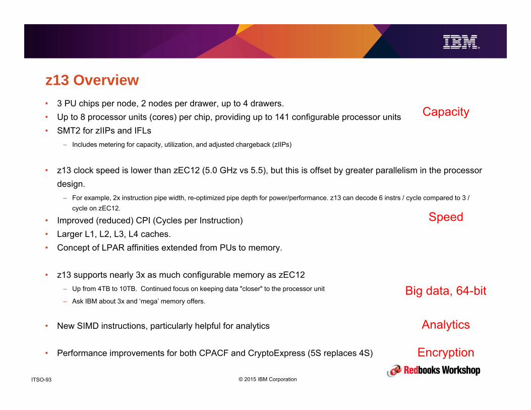
z13 Overview• 3 PU chips per node, 2 nodes per drawer, up to 4 drawers.• Up to 8 processor units (cores) per chip, providing up to 141 configurable processor units• SMT2 for zIIPs and IFLs
– Includes metering for capacity, utilization, and adjusted chargeback (zIIPs)
• z13 clock speed is lower than zEC12 (5.0 GHz vs 5.5), but this is offset by greater parallelism in the processor design.
– For example, 2x instruction pipe width, re-optimized pipe depth for power/performance. z13 can decode 6 instrs / cycle compared to 3 / cycle on zEC12.
• Improved (reduced) CPI (Cycles per Instruction)• Larger L1, L2, L3, L4 caches.• Concept of LPAR affinities extended from PUs to memory.
• z13 supports nearly 3x as much configurable memory as zEC12– Up from 4TB to 10TB. Continued focus on keeping data "closer" to the processor unit
– Ask IBM about 3x and ‘mega’ memory offers.
• New SIMD instructions, particularly helpful for analytics
• Performance improvements for both CPACF and CryptoExpress (5S replaces 4S)
Speed
Capacity
Big data, 64-bit
Analytics
Encryption

© 2015 IBM CorporationITSO-94
z13 PU Chip Up to eight active cores (PUs) per chip
–5.0 GHz (v5.5 GHz zEC12) –L1 cache/ core–L2 cache/ core
Single Instruction/Multiple Data (SIMD) Single thread or 2-way simultaneous
multithreaded (SMT) operation Improved instruction execution bandwidth:
–Greatly improved branch prediction and instruction fetch to support SMT
–Instruction decode, dispatch, complete increased to 6 instructions per cycle*
–Issue up to 10 instructions per cycle*–Integer and floating point execution units
On chip 64 MB eDRAM L3 Cache–Shared by all cores
I/O buses–One GX++ I/O bus–Two PCIe I/O buses
Memory Controller (MCU)–Interface to controller on memory DIMMs–Supports RAIM design
Chip Area– 678.8 mm2
– 28.4 x 23.9 mm– 17,773 power pins– 1,603 signal I/Os
14S0 22nm SOI Technology– 17 layers of metal– 3.99 Billion Transistors– 13.7 miles of copper wire
* zEC12 decodes 3 instructions and executes 7

© 2015 IBM CorporationITSO-95
z13 PU Core
CP Chip Floorplan
2X Instruction pipe width – Improves IPC for all modes– Symmetry simplifies dispatch/issue rules– Required for effective SMT
Added FXU and BFU execution units– 4 FXUs– 2 BFUs, – 2 DFUs,– 2 new SIMD units (VXUs)
SIMD unit plus additional registers Pipe depth re-optimized for
power/performance– Product frequency reduced– Processor performance increased
SMT support– Wide, symmetric pipeline– Full architected state per thread– SMT-adjusted CPU usage metering
IFB
ICMLSU
ISU
IDU
FXU
RU
L2DL2I
XUPC
VFU
COP
© 2015 IBM CorporationITSO-96
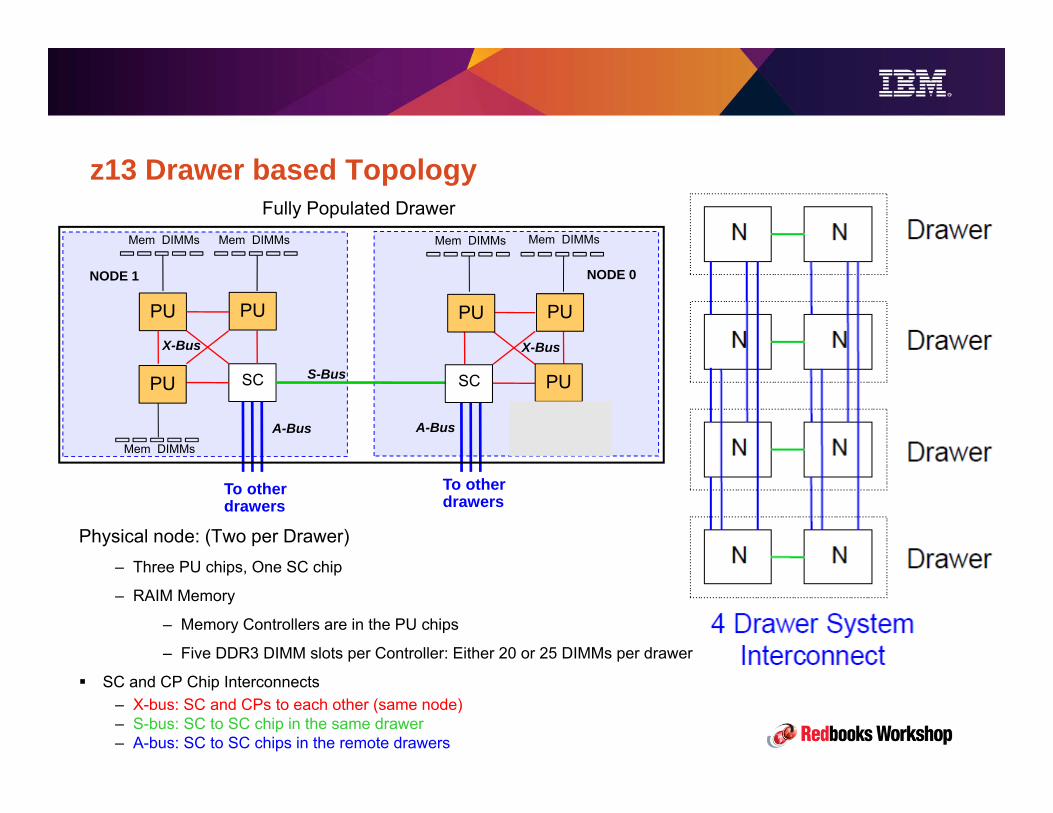
z13 Drawer based Topology
Mem DIMMsMem DIMMs
PUPU
SCSC
Mem DIMMs
NODE 1
Fully Populated Drawer
Mem DIMMsMem DIMMs
A-Bus
S-Bus
X-Bus
NODE 0
X-Bus
SCSC
A-Bus
To otherdrawers
To otherdrawers
PU
PU
PU PU
PU
Mem DIMMs
Physical node: (Two per Drawer)– Three PU chips, One SC chip
– RAIM Memory
– Memory Controllers are in the PU chips
– Five DDR3 DIMM slots per Controller: Either 20 or 25 DIMMs per drawer
SC and CP Chip Interconnects– X-bus: SC and CPs to each other (same node)– S-bus: SC to SC chip in the same drawer – A-bus: SC to SC chips in the remote drawers

© 2015 IBM CorporationITSO-97
zEC12 Book based Topology Fully connected 4 Book system:
120* total cores Total system cache
- 1536 MB shared L4 (eDRAM) (5632)- 576 MB L3 (eDRAM) (1536)- 144 MB L2 private (SRAM) (564)- 19.5 MB L1 private (SRAM) (31.5)
CP1CP1CP2CP2
CP4CP4 CP5CP5CP3CP3
SC0SC1
Mem1 Mem0
FBCs
Mem2
CP0CP0
Book:
FBCs
*Of the maximum 144 PUs only 120 are used

© 2015 IBM CorporationITSO-98
Comparing z13 structure with the zEC12 one• z13 hardware structure is significantly different than the z10/z196/zEC12 one – the step from
EC12 to z13 is similar to the step from z9 to z10:
– Every time System z has a major new design, some workloads will benefit more than others.
– The generations that are incremental refinements (e.g. zEC12 over z196) have less variability because they do
things the same way, only faster.
• z13 has direct point-to-point connectivity among processors in the same node. This was not
available in previous design.
• z13 has a fast bus (S-Bus) connecting the two nodes within the same drawer. This makes intra-
Drawer communication very efficient.
• z13 lacks any-to-any node connectivity which was available in previous design. This makes
communication between opposite nodes in different drawers (aka «far nodes») less efficient
than in the past.
• The new structure is needed to accomodate a larger number of processors (up from 101 to 141)
and provide growth.
© 2015 IBM CorporationITSO-99
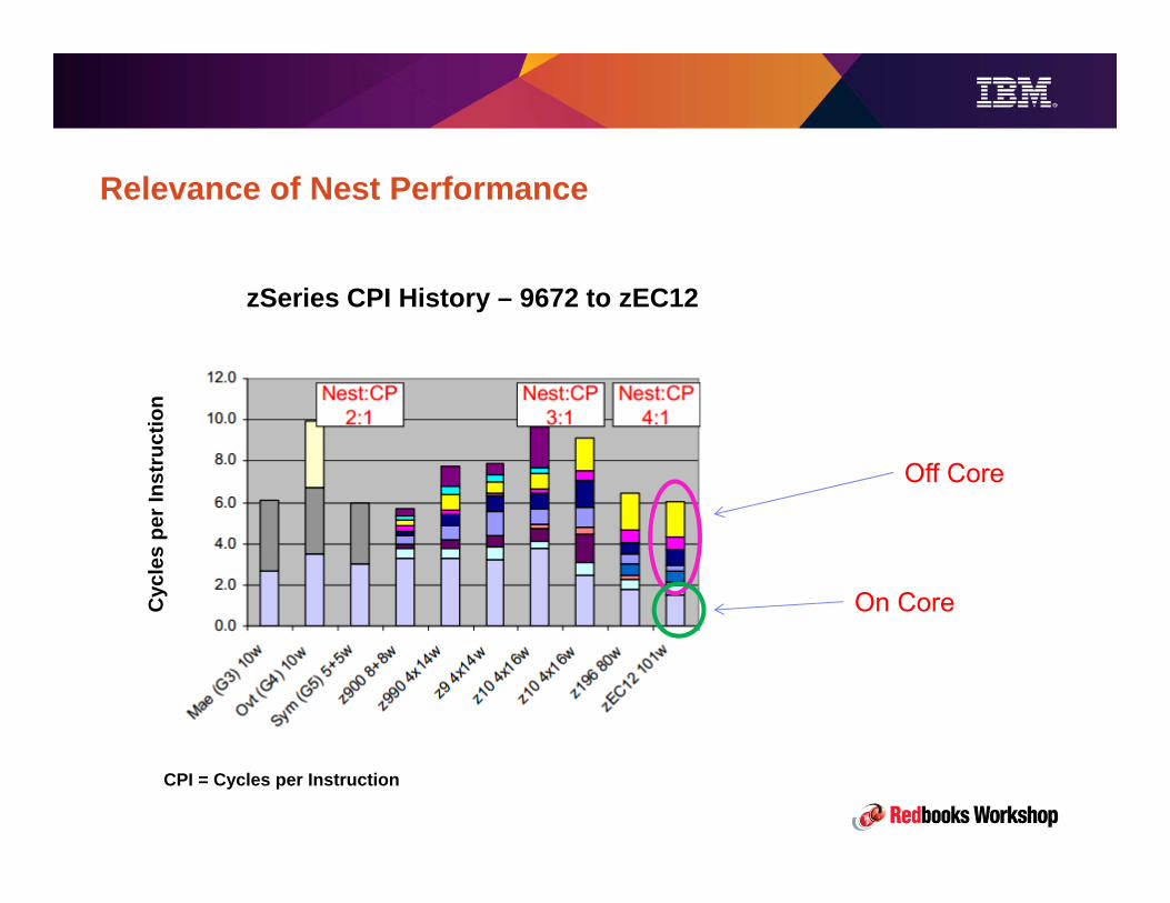
Relevance of Nest Performance
zSeries CPI History – 9672 to zEC12
Cyc
les
per I
nstr
uctio
n
CPI = Cycles per Instruction
Off Core
On Core

© 2015 IBM CorporationITSO-100
Impact of Relative Nest Intensity
50,000 MIPS difference!
30 engine difference!
© 2015 IBM CorporationITSO-101
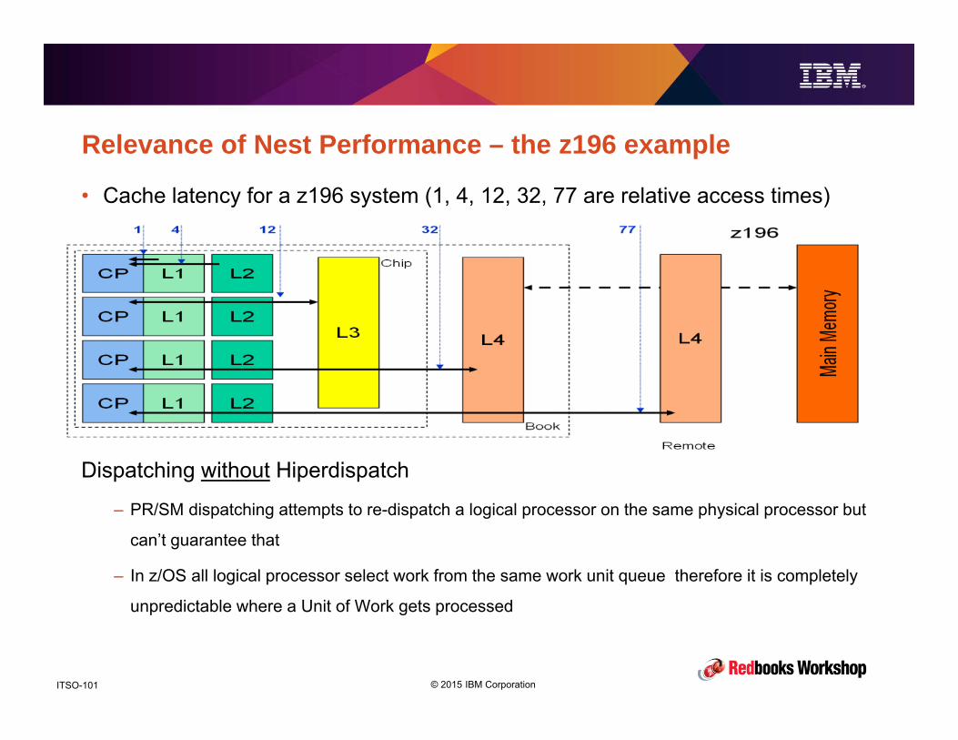
Relevance of Nest Performance – the z196 example
• Cache latency for a z196 system (1, 4, 12, 32, 77 are relative access times)
Dispatching without Hiperdispatch
– PR/SM dispatching attempts to re-dispatch a logical processor on the same physical processor but
can’t guarantee that
– In z/OS all logical processor select work from the same work unit queue therefore it is completely
unpredictable where a Unit of Work gets processed

© 2015 IBM CorporationITSO-102
Hiperdispatch design objectives and implementation
• HiperDispatch was introduced with z10
• Objective is to keep work as much as possible local to a physical processor to
optimize the usage of the processor caches. Expected result:
– Cache reloads should occur much less frequently
– Cache misses and fetches from other books (and chips) should be avoided as much as possible
• Implemented through the interaction between z/OS and PR/SM to optimize work
unit and logical processor placement to physical processors. Consists of 2 parts:
– One in z/OS (aka Dispatcher Affinity) because it attempts to create a temporary affinity between
work and processors
– One in PR/SM (aka Vertical CPU Management) because it attempts to assign physical processors
exclusively to logical processors as much as possible
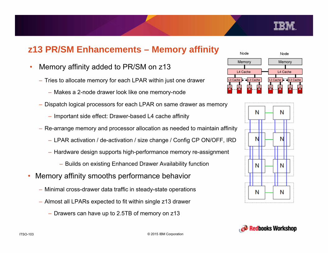
© 2015 IBM CorporationITSO-103
z13 PR/SM Enhancements – Memory affinity
• Memory affinity added to PR/SM on z13
– Tries to allocate memory for each LPAR within just one drawer
– Makes a 2-node drawer look like one memory-node
– Dispatch logical processors for each LPAR on same drawer as memory
– Important side effect: Drawer-based L4 cache affinity
– Re-arrange memory and processor allocation as needed to maintain affinity
– LPAR activation / de-activation / size change / Config CP ON/OFF, IRD
– Hardware design supports high-performance memory re-assignment
– Builds on existing Enhanced Drawer Availability function
• Memory affinity smooths performance behavior
– Minimal cross-drawer data traffic in steady-state operations
– Almost all LPARs expected to fit within single z13 drawer
– Drawers can have up to 2.5TB of memory on z13
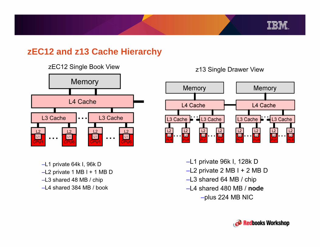
© 2015 IBM CorporationITSO-104
zEC12 and z13 Cache Hierarchy
...
Memory
L4 Cache
L2
CPU1L1
L3 Cache
L2
CPU6L1... L2
CPU1L1
L3 Cache
L2
CPU6L1...
zEC12 Single Book View z13 Single Drawer View
–L1 private 64k I, 96k D–L2 private 1 MB I + 1 MB D–L3 shared 48 MB / chip–L4 shared 384 MB / book
–L1 private 96k I, 128k D–L2 private 2 MB I + 2 MB D –L3 shared 64 MB / chip–L4 shared 480 MB / node
–plus 224 MB NIC

© 2015 IBM CorporationITSO-105
Workload’s Relative Nest Intensity Workload’s performance is sensitive to how deep into the memory hierarchy the processor must
go to retrieve workload’s instructions and data for execution. Best performance occurs when the instructions and data are found in the cache(s) nearest the processor (remember those relative access times on earlier slide).
To identify a workload profile, IBM introduced a new term, “Relative Nest Intensity (RNI)” which indicates the level of activity to shared cache and memory resources (L3, L4, memory). The higher the RNI, the deeper into the memory hierarchy the processor must go to retrieve the instructions and data for that workload.

© 2015 IBM CorporationITSO-106
A system’s Relative Nest Intensity varies with the workloadSample customer data – not z13
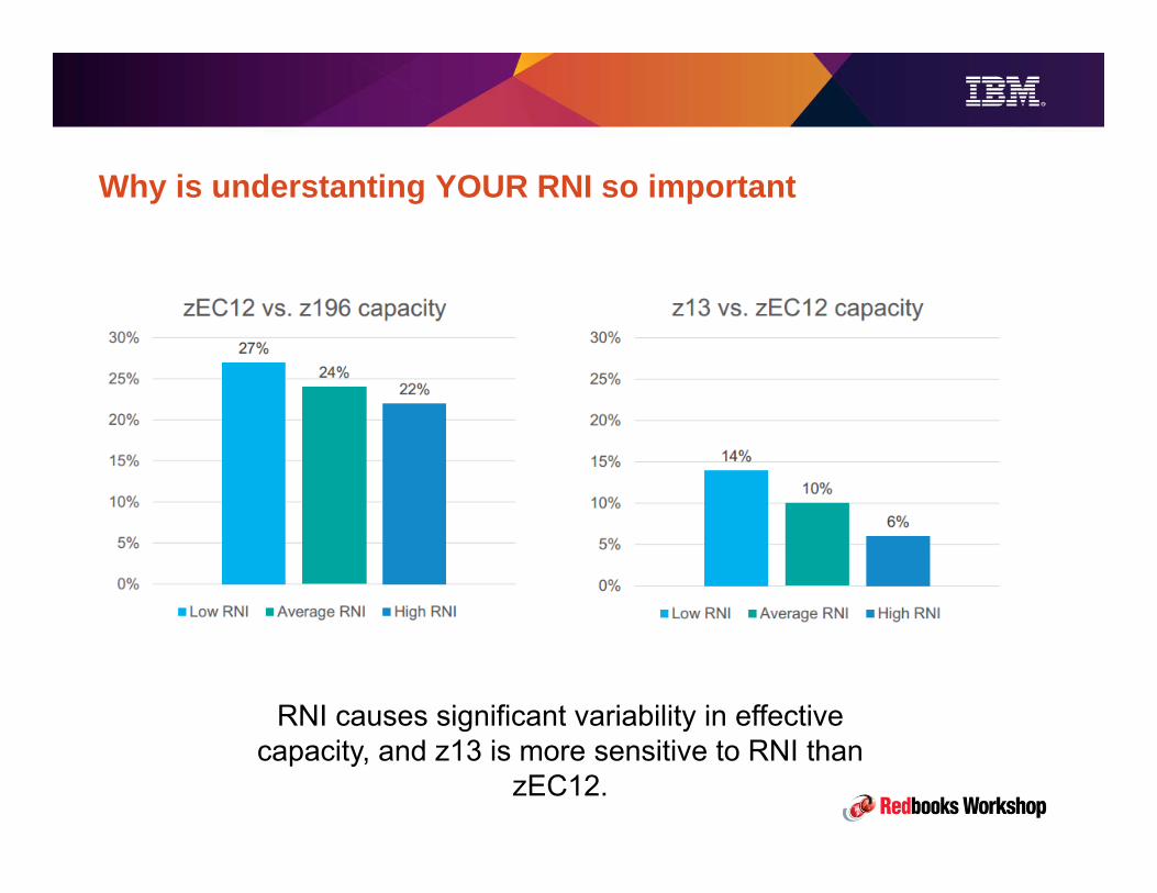
© 2015 IBM CorporationITSO-107
Why is understanting YOUR RNI so important
RNI causes significant variability in effective capacity, and z13 is more sensitive to RNI than
zEC12.

© 2015 IBM CorporationITSO-108
The importance of assigning the right LPAR weight
In HD mode, LPARs use Vertical Low logical processors to consume above guaranteed capacity
Sample customer data – not z13

© 2015 IBM CorporationITSO-109
The importance of assigning the right LPAR weight
• The previous chart shows a wee’sk worth of data about CPU consumption of a
production system – GSY7. In the chart, the blue line represents the processing
capacity assigned to the LPAR based on its weight. In many intervals GSY7
uses more than its guaranteed capacity. In HiperDispatch mode this is done
using Vertical Low logical processors. These processors use what’s left by other
LPARs and can be dispatched on any available physical processor.
• For this reason, Vertical Low logical processors, depending on the workload’s
relative nest intensity, show less cache efficiency. This is reflected in their CPI.
• Let us see the effect of cache efficiency on CPI using some customer data.
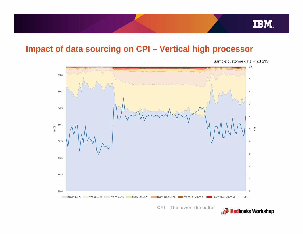
© 2015 IBM CorporationITSO-110
Impact of data sourcing on CPI – Vertical high processorSample customer data – not z13
CPI – The lower the better

© 2015 IBM CorporationITSO-111
Impact of data sourcing on CPI – Vertical high processor
• Vertical high logical processors are always dispatched on the same physical
processor. This increases the efficiency of L1 and L2 caches, which are private
to each PU (Processing Unit) and the L3 cache, which is located in the multi-
core PU chip.
• The previous chart shows how the CPI mainly depends on L1 cache efficiency,
but also shows how, for vertical high logical processors, most of the data
needed to keep processing is sourced by L1, L2 and L3 which are closer to the
processor.
• This is the effect of the persistent affinity generated by HiperDispatch for vertical
high processors.

© 2015 IBM CorporationITSO-112
Impact of data sourcing on CPI – Vertical medium processorSample customer data – not z13
CPI – The lower the better

© 2015 IBM CorporationITSO-113
Impact of data sourcing on CPI – Vertical medium processor• Vertical medium logical processors are assigned a home physical processor of
which they own a significant share. However, unlike vertical highs, they can be
dispatched elsewhere by PR/SM should the home physical processor be busy when
needed.
• PR/SM knows the CEC’s hardware topology, and keeps track of where logical
processors have been previously dispatched. This allows it to try to maximize cache
efficiency when it needs to dispatch a logical processor on a PU different than its
home one.
• In the previous chart we see that the medium processor has less L3 cache efficiency
than the vertical high one, but that it enjoys a good L4 efficiency. L4 is shared by
PUs in the same Book / Drawer.

© 2015 IBM CorporationITSO-114
Impact of data sourcing on CPI – Vertical low processorSample customer data – not z13
CPI – The lower the better

© 2015 IBM CorporationITSO-115
Impact of data sourcing on CPI – Vertical low processor
• Vertical low logical processors are usually parked and are not used until the LPAR
needs more capacity than it is allowed by its relative share. Vertical low processors
are dispatched wherever there are available cycles (in any drawer). This results in
them having lower cache hit rates AND in polluting caches of other logical
processors. Because it is difficult for PR/SM to maximize cache efficiency for
vertical low logical processors, their RNI (and hence their performance) tends to be
much less consistent than vertical mediums or vertical highs.
• In the previous chart you can see how vertical low processors show less cache
efficiency from shared caches (L3 and L4) because they keep moving between chips
and drawers. Their CPI is highly dependent on L1 and L2, which in turn depend on
the data locality of the workload.

© 2015 IBM CorporationITSO-116
Things you may consider to maximize performance• Be aware of your workload’s cache profile, use CPU MF (SMF Type 113 records) data
to determine it and tools such as zPCR or SAS/MXG to plot and monitor its use of
cache.
• Assign your LPARs the right processor weight. Try to make sure that vertical low
logical processors are seldomly used.– If possible assign a processor weight that makes PR/SM use as many Vertical high processors as possible.
Use Alain’s Maneville excellent LPAR Design tool To plan your LPAR configuration.
http://www-03.ibm.com/systems/z/os/zos/features/wlm/WLM_Further_Info_Tools.html#Design
• Try to not saturate your physical processing capacity. If possible, over-provision it, as
lower CPU utilization brings more efficiency and has a potential for cost reduction.
See IBM White Paper WP101208 – ‘Running IBM System z at High Utilization’ by
Gary King.– Also consider the use of subcapacity models.
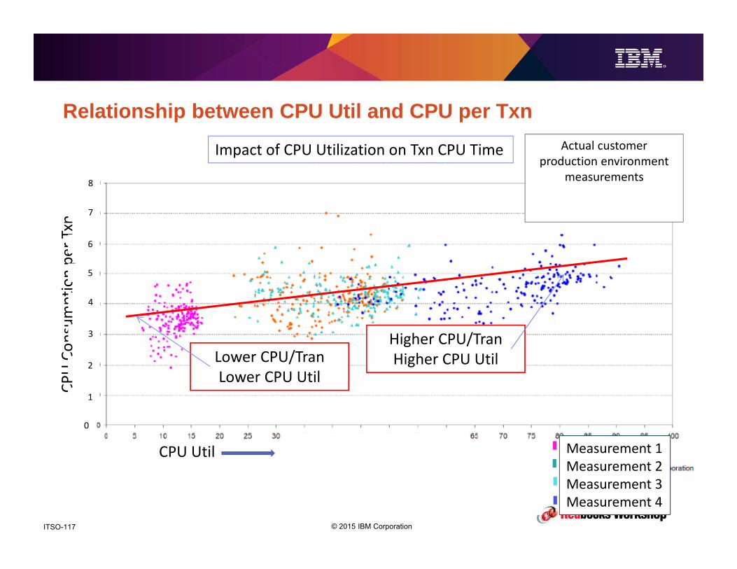
© 2015 IBM CorporationITSO-117
Relationship between CPU Util and CPU per Txn
•
CPU Util
CPU
Con
sum
ptio
n pe
r Txn
Actual customer production environment
measurements
Lower CPU/TranLower CPU Util
Higher CPU/TranHigher CPU Util
Impact of CPU Utilization on Txn CPU Time
0
1
2
3
4
5
6
7
8
Measurement 1Measurement 2Measurement 3Measurement 4

© 2015 IBM CorporationITSO-118
Things you may consider to maximize performance
• Try to minimize cache disruptions due to interrupts. Larger memory
configurations allow for fewer I/Os and better RNIs. – Consider using DB2 page-fixed Buffer Pools and large (1MB) pages.
– z13 supports larger memory configurations. But try to ensure that each LPAR’s memory fits in a
single drawer.
• Increase TLB efficiency by using Large Pages. This is especially important
when moving to larger memory configurations.– 1MB pages use a separate TLB and take pressure off the 4KB TLB.
– Make sure you have enough real memory to avoid RSM breaking up large pages to back 4K ones.
• If using sysplex data sharing, aim to maximize proportion of synchronous
requests. Make use of the fastest available link technology.– ICA on z13 and CIB 12X-IFB3 on zEC12 for short distances, CIB 1X for long distances.

© 2015 IBM CorporationITSO-119
z13 Memory Location
Source: z13 Technical Guide - http://www.redbooks.ibm.com/abstracts/sg248251.html?Open
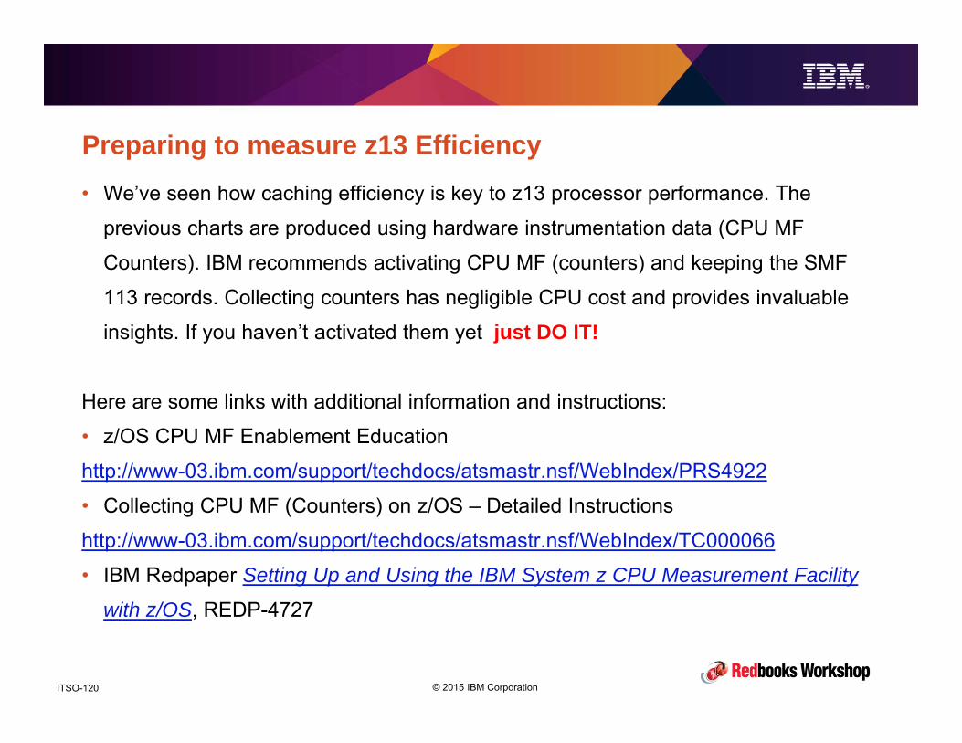
© 2015 IBM CorporationITSO-120
Preparing to measure z13 Efficiency• We’ve seen how caching efficiency is key to z13 processor performance. The
previous charts are produced using hardware instrumentation data (CPU MF
Counters). IBM recommends activating CPU MF (counters) and keeping the SMF
113 records. Collecting counters has negligible CPU cost and provides invaluable
insights. If you haven’t activated them yet just DO IT!
Here are some links with additional information and instructions:
• z/OS CPU MF Enablement Education
http://www-03.ibm.com/support/techdocs/atsmastr.nsf/WebIndex/PRS4922
• Collecting CPU MF (Counters) on z/OS – Detailed Instructions
http://www-03.ibm.com/support/techdocs/atsmastr.nsf/WebIndex/TC000066
• IBM Redpaper Setting Up and Using the IBM System z CPU Measurement Facility
with z/OS, REDP-4727
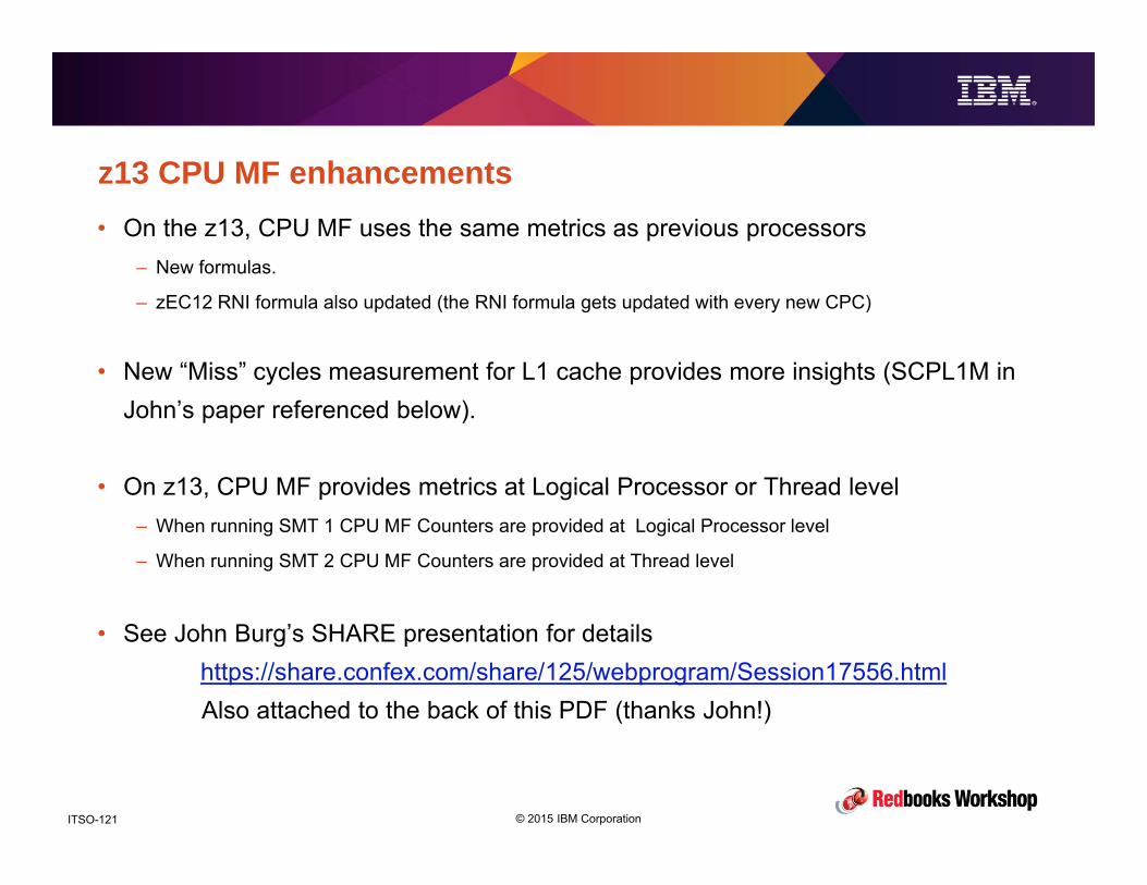
© 2015 IBM CorporationITSO-121
z13 CPU MF enhancements• On the z13, CPU MF uses the same metrics as previous processors
– New formulas.
– zEC12 RNI formula also updated (the RNI formula gets updated with every new CPC)
• New “Miss” cycles measurement for L1 cache provides more insights (SCPL1M in John’s paper referenced below).
• On z13, CPU MF provides metrics at Logical Processor or Thread level– When running SMT 1 CPU MF Counters are provided at Logical Processor level
– When running SMT 2 CPU MF Counters are provided at Thread level
• See John Burg’s SHARE presentation for detailshttps://share.confex.com/share/125/webprogram/Session17556.htmlAlso attached to the back of this PDF (thanks John!)

© 2015 IBM CorporationITSO-122
Understanding your LPARs’ topology
• Assigning proper weights lets you influence the number of vertical high/medium
processors a LPAR will use.
– Use Alain Maneville’s LPAR Design tool.
• In a z13 configuration, aim to have all logical processors and memory for a
given LPAR fit in a single drawer.
• To see how successful you are with this, you need to know how physical
memory and Processor Units are distributed across drawers, and how PR/SM
allocates home PUs to logical processors.
– Logical processor topology information can be obtained by using SMF99.14.
– There is no way to determine actual in-use memory in each drawer.
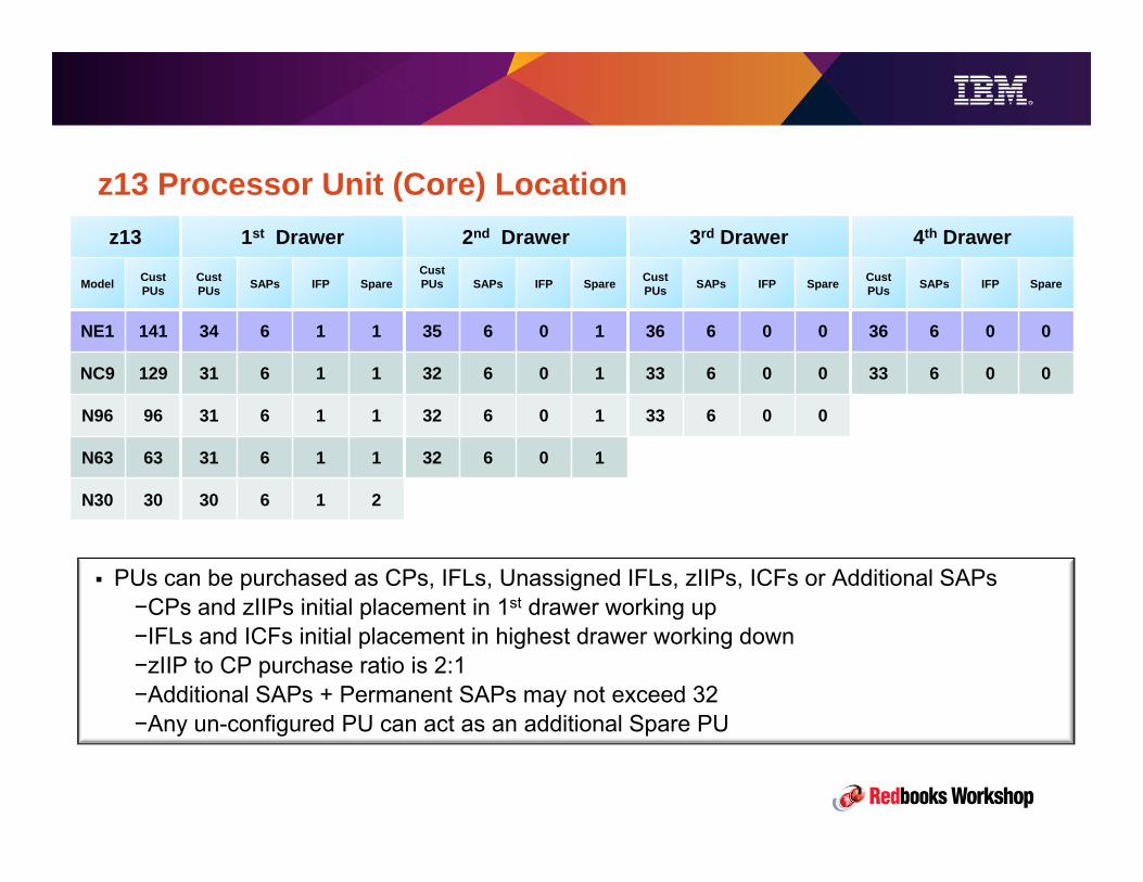
© 2015 IBM CorporationITSO-123
z13 Processor Unit (Core) Location
PUs can be purchased as CPs, IFLs, Unassigned IFLs, zIIPs, ICFs or Additional SAPs−CPs and zIIPs initial placement in 1st drawer working up−IFLs and ICFs initial placement in highest drawer working down −zIIP to CP purchase ratio is 2:1−Additional SAPs + Permanent SAPs may not exceed 32−Any un-configured PU can act as an additional Spare PU
z13 1st Drawer 2nd Drawer 3rd Drawer 4th Drawer
Model CustPUs
CustPUs SAPs IFP Spare
CustPUs SAPs IFP Spare Cust
PUs SAPs IFP Spare CustPUs SAPs IFP Spare
NE1 141 34 6 1 1 35 6 0 1 36 6 0 0 36 6 0 0
NC9 129 31 6 1 1 32 6 0 1 33 6 0 0 33 6 0 0
N96 96 31 6 1 1 32 6 0 1 33 6 0 0
N63 63 31 6 1 1 32 6 0 1
N30 30 30 6 1 2
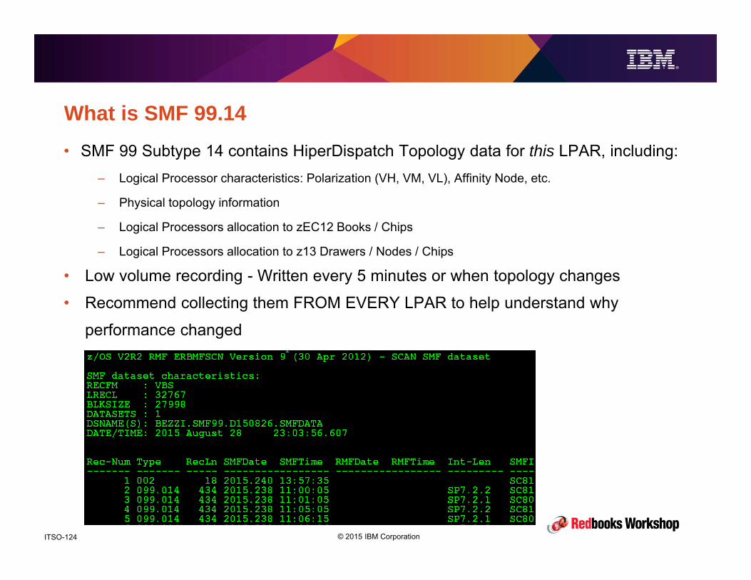
© 2015 IBM CorporationITSO-124
What is SMF 99.14• SMF 99 Subtype 14 contains HiperDispatch Topology data for this LPAR, including:
– Logical Processor characteristics: Polarization (VH, VM, VL), Affinity Node, etc.
– Physical topology information
– Logical Processors allocation to zEC12 Books / Chips
– Logical Processors allocation to z13 Drawers / Nodes / Chips
• Low volume recording - Written every 5 minutes or when topology changes
• Recommend collecting them FROM EVERY LPAR to help understand why
performance changed

© 2015 IBM CorporationITSO-125
The WLM Topology Reporter
New WLM Topology Report available to process SMF 99 subtype 14 records
http://www-03.ibm.com/systems/z/os/zos/features/wlm/WLM_Further_Info_Tools.html#Topology
Steps:1. Download tool from web site above2. Collect SMF 99 Subytpe 14 records3. Run provided host program to create topology file in CSV format4. Download topology file to workstation5. Load it into provided Excel spreadsheet to generate topology reports

© 2015 IBM CorporationITSO-126
WLM Topology Reporter

© 2015 IBM CorporationITSO-127
WLM Topology Reporter - Spreadsheet
1 – Create copy of current spreadsheet
2 – Open CSV file containing
SMF99.14 data
3 – Select Interval to be analyzed 4 – Copy data into
main sheet 5 – Create Report

© 2015 IBM CorporationITSO-128
WLM Topology Reporter – Interpreting the results

© 2015 IBM CorporationITSO-129
WLM Topology Reporter – Sample use case
• In the following slides, we’ll see an example of a Topology Report and review
how it can be used to understand what happens during a system’s
reconfiguration.
• To do this we started with a z13 LPAR configuration using 6 dedicated CPs and
8 dedicated zIIPs and dynamically varied online another zIIP.
– NOTE: While the Type 113 records provide information at the thread level (when running in SMT2
mode), the 99.14 records are at the core level.
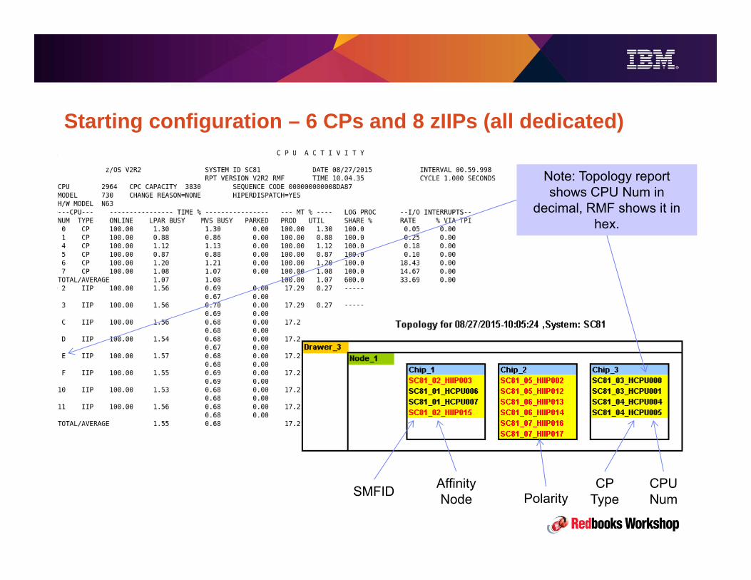
© 2015 IBM CorporationITSO-130
Starting configuration – 6 CPs and 8 zIIPs (all dedicated)
SMFID Affinity Node Polarity
CP Type
CPU Num
Note: Topology report shows CPU Num in
decimal, RMF shows it in hex.
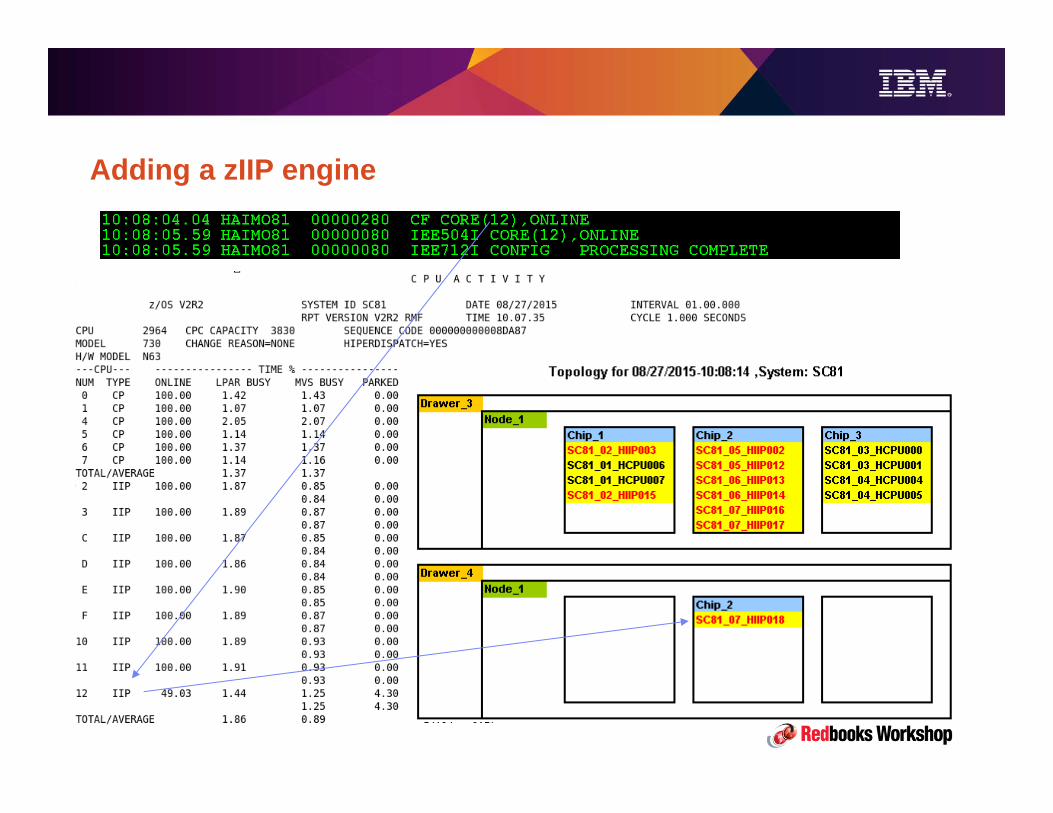
© 2015 IBM CorporationITSO-131
Adding a zIIP engine

© 2015 IBM CorporationITSO-132
PR/SM reaction – Dynamic Processor ReassignmentAfter a while (up to 5 mins), PR/SM performs dynamic processor reassignment to move the last added zIIP to the same node where other processors of the same system reside

© 2015 IBM CorporationITSO-133
Z13 Performance topics summary
• Be familiar with your workload’s cache profile so that you can spot unexpected
changes or the impact of tuning efforts. – Collect CPU MF Counters, use CPU MF data to determine your workload profile.
• Assign your LPARs the right processor weight to maximize use of VH and VM CPs.
– Get familiar with LPAR Design Tool, SMF99.14 and WLM Topology Reporter
• If possible, over-provision CPU capacity as it can bring more efficiency.
• Exploit larger memory configurations and attractive pricing to reduce I/O and
improve RNI.
• Implement Large Pages to increase TLB efficiency.
• For sysplex data sharing, make use of the fastest available link technology.
© 2015 IBM CorporationITSO-134
New z13 Single Instruction Multiple Data instructions
Performance and Availability

© 2015 IBM CorporationITSO-135
Introduction
• z13 is the first System z CEC providing specialized hardware to improve the
performance of complex mathematical models and analytic workloads through
vector processing and new complex instructions, which can process multiple
data items with only a single instruction.
• This section will give you introductory information about SIMD, including
motivations, implementation, exploiters, and performance.
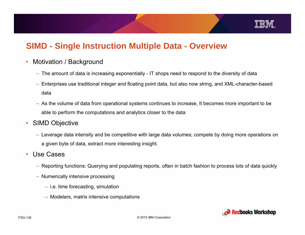
© 2015 IBM CorporationITSO-136
SIMD - Single Instruction Multiple Data - Overview
• Motivation / Background
– The amount of data is increasing exponentially - IT shops need to respond to the diversity of data
– Enterprises use traditional integer and floating point data, but also now string, and XML-character-based
data
– As the volume of data from operational systems continues to increase, It becomes more important to be
able to perform the computations and analytics closer to the data
• SIMD Objective
– Leverage data intensity and be competitive with large data volumes; compete by doing more operations on
a given byte of data, extract more interesting insight.
• Use Cases
– Reporting functions: Querying and populating reports, often in batch fashion to process lots of data quickly
– Numerically intensive processing
– i.e. time forecasting, simulation
– Modelers, matrix intensive computations

© 2015 IBM CorporationITSO-137
Instruction pool Data pool
Results
Instruction pool Data pool
Results
WorkloadsJava.Next C/C++Compiler built-ins
for SIMD operations (z/OS and Linux on z
Systems)
MASS & ATLASMath Libraries
(z/OS and Linux on z Systems)
SIMD Registers and Instruction Set
MASS - Mathematical Acceleration Sub-SystemATLAS - Automatically Tuned Linear Algebra Software
Single Instruction Multiple Data (SIMD) Vector Processing A type of data parallel computing that can accelerate operations on integer, string, character, and
floating point data types
Provide optimized SIMD compliers and libraries that will minimize the effort on the part of middleware/application developers
Operating System/Hypervisor Support:− z/OS: 2.1 SPE available at GA− Compiler exploitation
• IBM Java V8 => 1Q2015• XL C/C++ on zOS => 1Q2015• XL C/C++ on Linux on z => 2Q2015• Enterprise COBOL => 1Q2015• Enterprise PL/I => 1Q2015
− Linux: IBM is working with its Linux Distribution partners to support new functions/features − No z/VM Support for SIMD
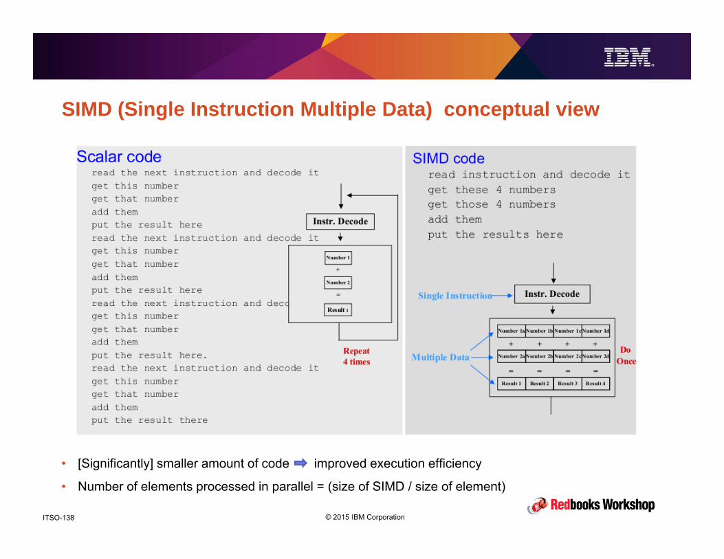
© 2015 IBM CorporationITSO-138
SIMD (Single Instruction Multiple Data) conceptual view
• [Significantly] smaller amount of code improved execution efficiency
• Number of elements processed in parallel = (size of SIMD / size of element)
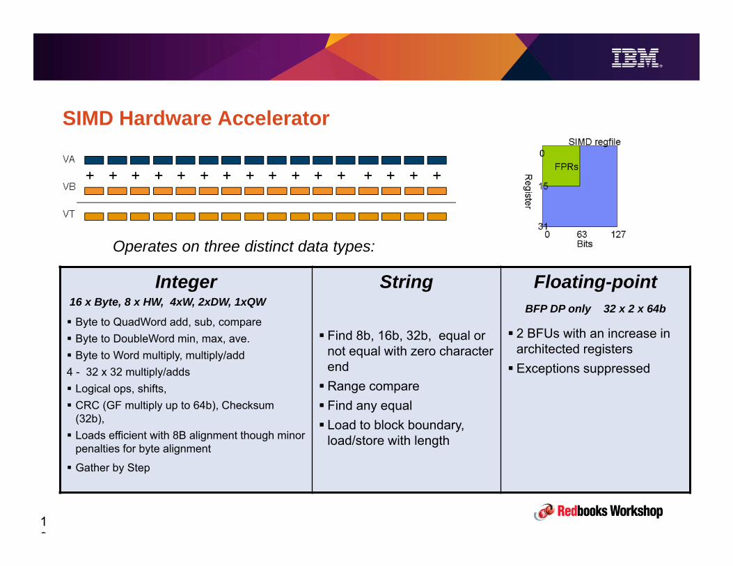
© 2015 IBM CorporationITSO-139
SIMD Hardware Accelerator
13
Integer16 x Byte, 8 x HW, 4xW, 2xDW, 1xQW
Byte to QuadWord add, sub, compare Byte to DoubleWord min, max, ave. Byte to Word multiply, multiply/add 4 - 32 x 32 multiply/adds Logical ops, shifts, CRC (GF multiply up to 64b), Checksum
(32b), Loads efficient with 8B alignment though minor
penalties for byte alignment
Gather by Step
String
Find 8b, 16b, 32b, equal or not equal with zero character endRange compare Find any equal Load to block boundary,
load/store with length
Floating-point BFP DP only 32 x 2 x 64b
2 BFUs with an increase in architected registers Exceptions suppressed
Operates on three distinct data types:
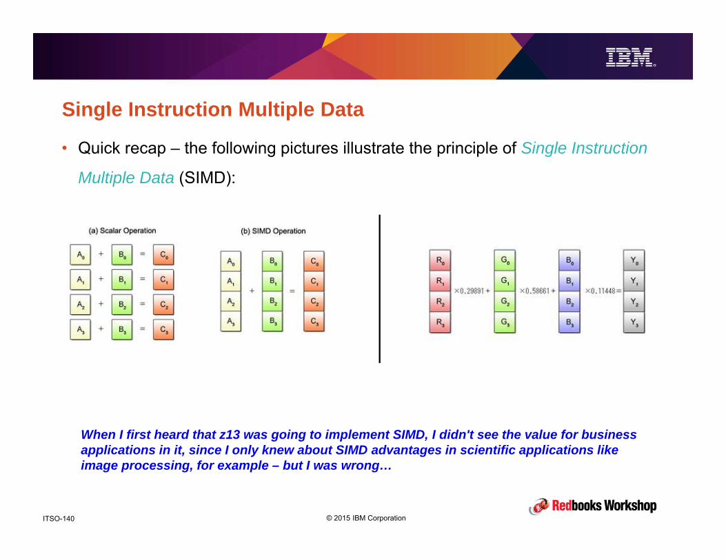
© 2015 IBM CorporationITSO-140
Single Instruction Multiple Data
• Quick recap – the following pictures illustrate the principle of Single Instruction
Multiple Data (SIMD):
When I first heard that z13 was going to implement SIMD, I didn't see the value for business applications in it, since I only knew about SIMD advantages in scientific applications like image processing, for example – but I was wrong…
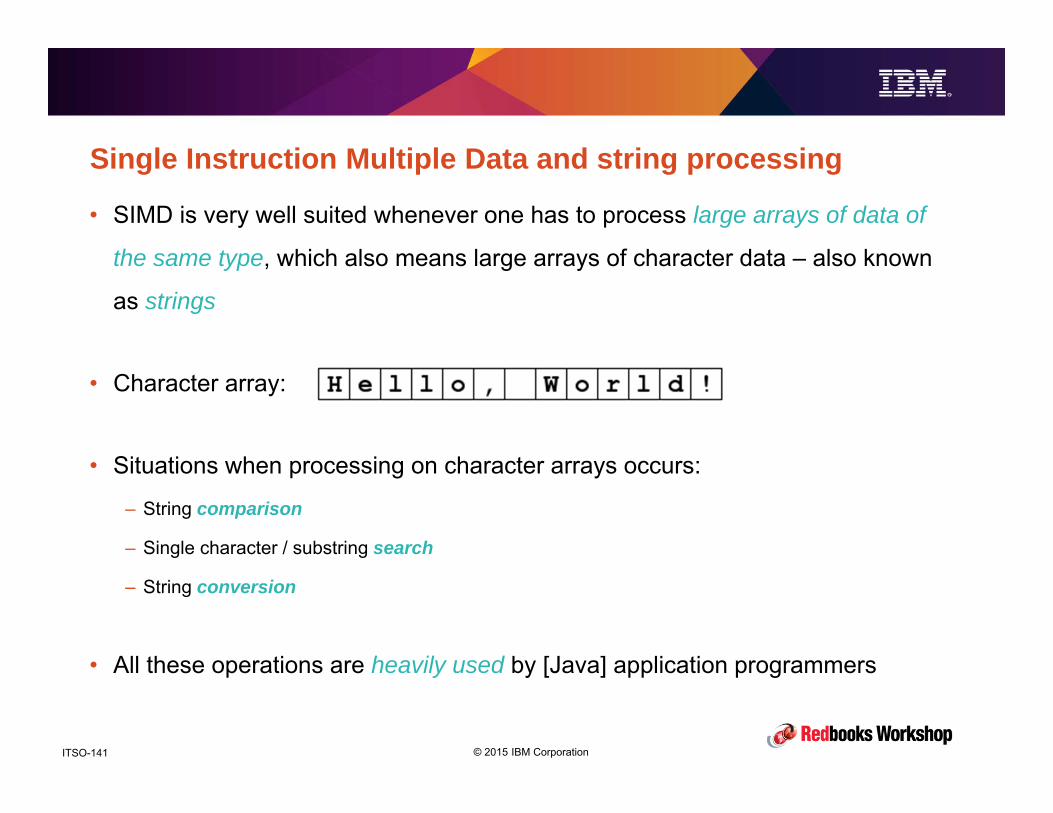
© 2015 IBM CorporationITSO-141
Single Instruction Multiple Data and string processing
• SIMD is very well suited whenever one has to process large arrays of data of
the same type, which also means large arrays of character data – also known
as strings
• Character array:
• Situations when processing on character arrays occurs:
– String comparison
– Single character / substring search
– String conversion
• All these operations are heavily used by [Java] application programmers

© 2015 IBM CorporationITSO-142
Java acceleration with SIMD
IBM z13 running Java 8 on z/OS®
Single Instruction Multiple Data (SIMD) vector engine exploitation
java.lang.String exploitation- compareTo- compareToIgnoreCase- contains- contentEquals- equals- indexOf- lastIndexOf- regionMatches- toLowerCase- toUpperCase- getBytes
java.util.Arrays- equals (primitive types)
String encoding converters For ISO8859-1, ASCII, UTF8, and UTF16- encode (char2byte)- decode (byte2char)
Auto-SIMD- Simple loops
(eg. matrix multiplication)

© 2015 IBM CorporationITSO-143
Java Sample – Read a large text file into a string 10,000 times

© 2015 IBM CorporationITSO-144
Java Sample – Same as before plus perform case conversion
The «toLower» method translates the text string to lower cases.When running on z13 Java 8 exploits SIMD to do it
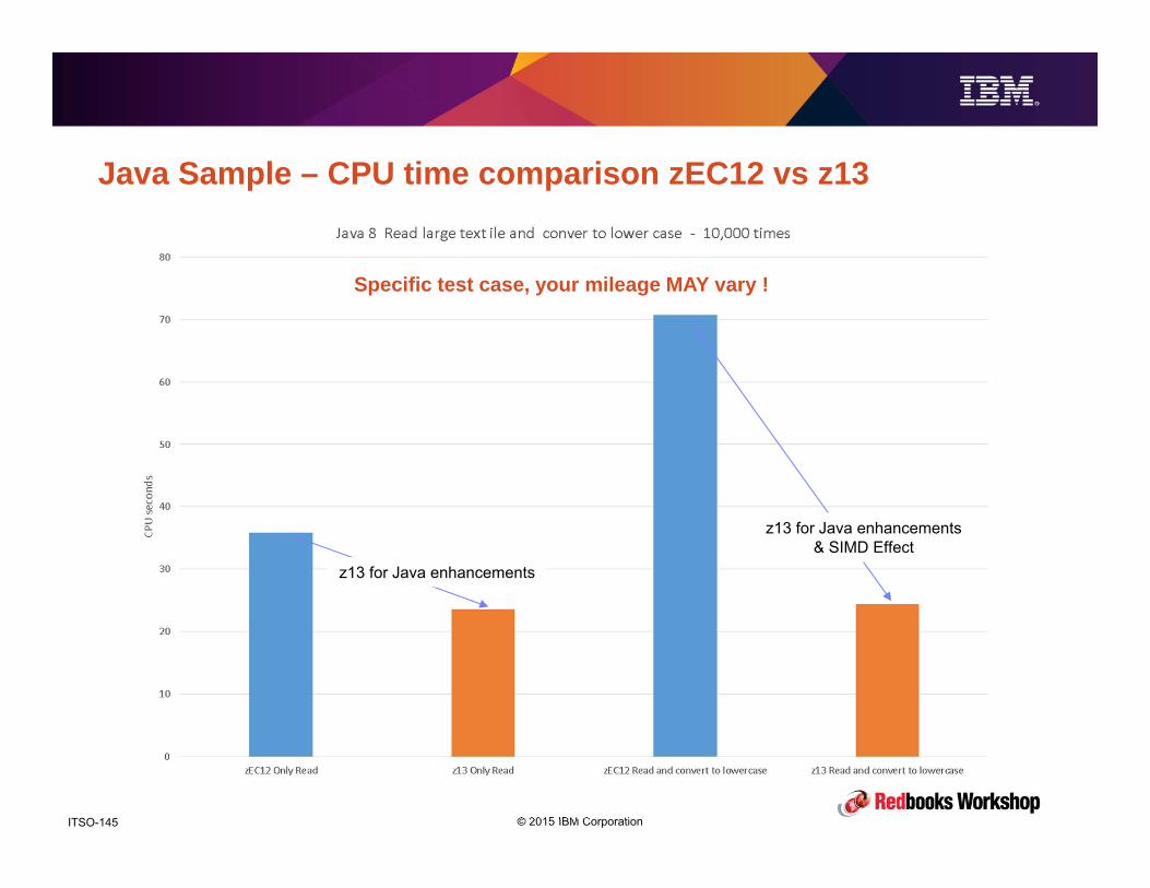
© 2015 IBM CorporationITSO-145
Java Sample – CPU time comparison zEC12 vs z13
z13 for Java enhancements& SIMD Effect
z13 for Java enhancements
Specific test case, your mileage MAY vary !
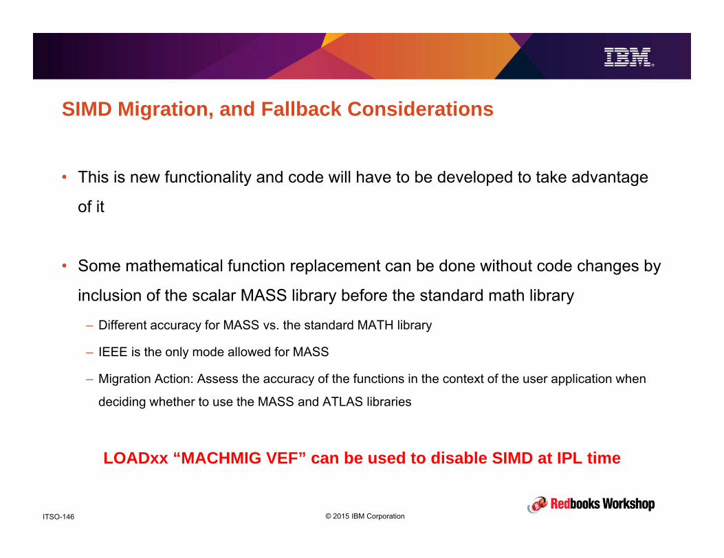
© 2015 IBM CorporationITSO-146
SIMD Migration, and Fallback Considerations
• This is new functionality and code will have to be developed to take advantage
of it
• Some mathematical function replacement can be done without code changes by
inclusion of the scalar MASS library before the standard math library
– Different accuracy for MASS vs. the standard MATH library
– IEEE is the only mode allowed for MASS
– Migration Action: Assess the accuracy of the functions in the context of the user application when
deciding whether to use the MASS and ATLAS libraries
LOADxx “MACHMIG VEF” can be used to disable SIMD at IPL time

© 2015 IBM CorporationITSO-147
SIMD enabled products• SIMD helps z Systems bringing analytics processing to the operational data
– Enables new workload growth and development on z
– Makes porting analytics workloads from the distributed/LOB analytics environments more actrattive
Area Product Description
SIMD Optimized Workloadsz/OS XMLSS XML ParsingILOG-CPLEX Mathematical optimization solverJava Workloads with string character or floating point data types
Enabling Libraries Rational Compiler Suite MASS Library on z/OS, Linux on z SystemsATLAS Library on z/OS, Linux on z Systems
Enabling Compilers / Built-in Functions (String, Integer, Floating Point Processing)
SIMD XLC for z/OS SIMD XLC Intrinsic and vector data types
GCC Compiler, Linux Kernel /Runtimes Default Linux C Compiler; SIMD context save/restore support, binutils, glibc
Enterprise COBOL for z/OS COBOL intrinsics (INSPECT), string processing facilitiesJava8 Compiler Java string character conversions, auto-vectorizationPL/I Optimizer and checkout compiler
ToolsLinux gdb Debugger for Linux OS ProgramsPD Tools (Fault Analyzer, Debug Tool,Application Performance Analyzer)
Source level Debugger for z/OS C, C++ Programs

© 2015 IBM CorporationITSO-148
Summary
• SIMD addresses what used to be a niche space, but is increasingly becoming
mainstream as companies make more use of ‘Big Data’.
• Key system components like Java and XML System Services have been
enabled to exploit SIMD for commonly used string processing functions.
• Custom exploitation requires changing your applications as with traditional
languages as COBOL and C automatic SIMD exploitation only applies to very
specific cases.
• If you are running Java on your z/OS system, especially with heavy string
processing, expect significant saving when moving to Java 8 on z13.

© 2015 IBM CorporationITSO-149
z13 Simultaneous Multi- ThreadingPerformance and Availability

© 2015 IBM CorporationITSO-150
Simultaneous Multi Threading Basics
© 2015 IBM CorporationITSO-151
Introduction
z13 is the first System z CEC implementing Simultaneous Multi Threading.
Simultaneous Multithreading (SMT) is a technique for increasing the efficiency of CPUs to
deliver more throughput per processor core. It has been exploited by distributed systems for
many years.
It builds on top of a number of other sophisticated mechanisms developed to increase
processing capacity by increasing the level of execution parallelism.
In the following few slides we will review how processor’s technology has evolved over time
to provide more processing capacity by increasing hardware efficiency.
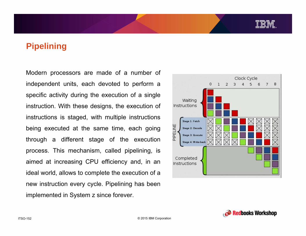
© 2015 IBM CorporationITSO-152
Pipelining
Modern processors are made of a number of
independent units, each devoted to perform a
specific activity during the execution of a single
instruction. With these designs, the execution of
instructions is staged, with multiple instructions
being executed at the same time, each going
through a different stage of the execution
process. This mechanism, called pipelining, is
aimed at increasing CPU efficiency and, in an
ideal world, allows to complete the execution of a
new instruction every cycle. Pipelining has been
implemented in System z since forever.
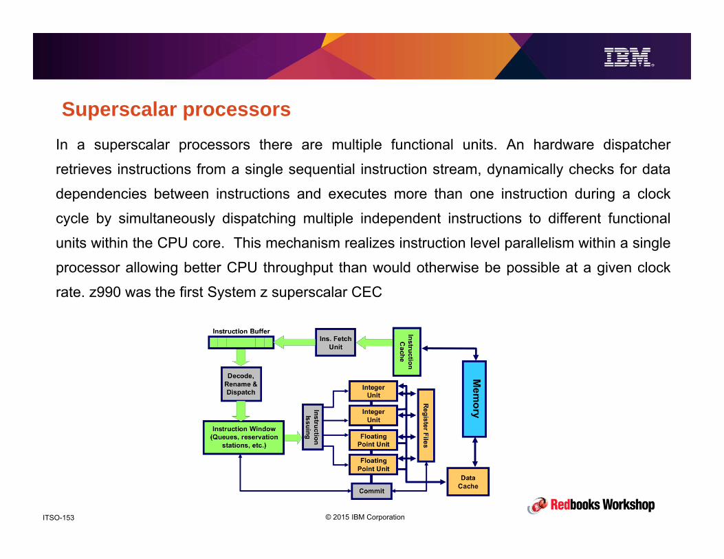
© 2015 IBM CorporationITSO-153
Superscalar processorsIn a superscalar processors there are multiple functional units. An hardware dispatcher
retrieves instructions from a single sequential instruction stream, dynamically checks for data
dependencies between instructions and executes more than one instruction during a clock
cycle by simultaneously dispatching multiple independent instructions to different functional
units within the CPU core. This mechanism realizes instruction level parallelism within a single
processor allowing better CPU throughput than would otherwise be possible at a given clock
rate. z990 was the first System z superscalar CEC
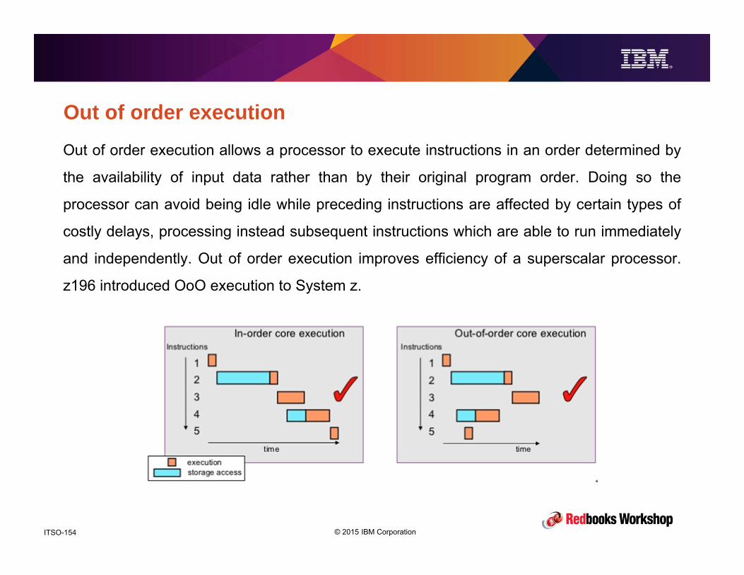
© 2015 IBM CorporationITSO-154
Out of order executionOut of order execution allows a processor to execute instructions in an order determined by
the availability of input data rather than by their original program order. Doing so the
processor can avoid being idle while preceding instructions are affected by certain types of
costly delays, processing instead subsequent instructions which are able to run immediately
and independently. Out of order execution improves efficiency of a superscalar processor.
z196 introduced OoO execution to System z.

© 2015 IBM CorporationITSO-155
Simultaneous Multi ThreadingSimultaneous multithreading (SMT) is a technique for improving the overall efficiency of
superscalar CPUs by implementing hardware multithreading. SMT permits multiple
independent threads of execution to better utilize the resources provided by modern
processor architectures. In simultaneous multithreading, instructions from more than one
thread can be executed by a single CPU core in any given pipeline stage at a time making
more efficient use of core hardware and increasing core's throughput. Z13 is the first
System z CEC implementing SMT.
© 2015 IBM CorporationITSO-156
z13 SMT

© 2015 IBM CorporationITSO-157
Why SMT is relevant to System z
• Increasing system performance needs more CPs and/or higher frequencies
and/or less cycles per instruction (CPI), however higher frequencies are more
and more difficult to achieve.
– That's why nowadays development efforts focus on execution parallelism and CPI reduction
• SMT enables continued scaling of per-processor capacity
– Multiple programs (software threads) run on the same processor core
– More efficient use of the core hardware
• SMT Increases per-core and system throughput versus single thread design
– More work done per unit hardware
– But each thread runs more slowly than on a single-thread core
– Aligns with industry direction of multi-threading

© 2015 IBM CorporationITSO-158
z13 SMT implementation
• z13 is the first System z Processor to support SMT
– z13 supports 2 threads per core on IFLs and zIIPs only
– Two programs (software threads) run on the same processor core
• Design allows dynamic independent enablement of SMT by LPAR
– Operating systems must be explicitly enabled for SMT
– Operating system may opt to run in single-thread mode
– Processors can run in single-thread operation for workloads needing maximum thread speed
• Functionally transparent to middleware and applications
– No changes required to run in SMT partition
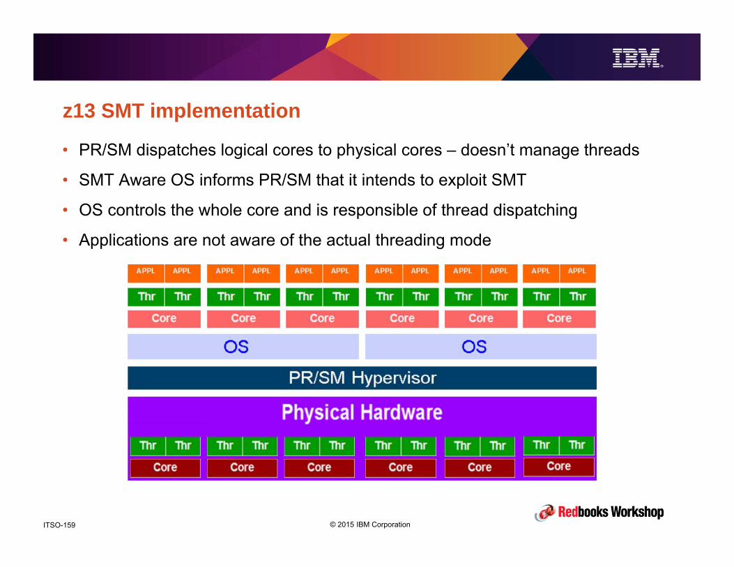
© 2015 IBM CorporationITSO-159
z13 SMT implementation
• PR/SM dispatches logical cores to physical cores – doesn’t manage threads
• SMT Aware OS informs PR/SM that it intends to exploit SMT
• OS controls the whole core and is responsible of thread dispatching
• Applications are not aware of the actual threading mode

© 2015 IBM CorporationITSO-160
z13 SMT expectations with z/OS – Your Mileage WILL vary!
• Expect zIIP cores running in SMT2 being able to do 0% to 40% more work than
when running single thread.
• When running SMT2 expect each zIIP thread being 0% to 30% slower than
when running single thread.
• Different workloads and different workload mixes show different throughput
gains and thread slow downs.
• z/OS v2 introduced a new metering system to allow using existing capacity
planning and charge back when running in SMT mode.

© 2015 IBM CorporationITSO-161
New z/OS terminology for SMT
• z/OS logical processor (CPU) -> Thread
– A thread implements (most of) the System z processor architecture
– When running in MT1 or MT2 mode z/OS dispatches work units on threads
– In MT2 mode two threads are mapped to a logical core
• Processor -> Core
– PR/SM dispatches logical cores on physical cores
– Thread density 1 (TD1) when only a single thread runs on a core
– Thread density 2 (TD2) when both threads run on a core

© 2015 IBM CorporationITSO-162
Exploiting SMT under z/OS
• z/OS SMT exploitation requires z/OS 2.1 + APARs or z/OS 2.2
• For z/OS to switch between CPU and CORE mode an IPL is needed
– LOADxx PROCVIEW CPU | CORE statement controls how z/OS will work for the life of the IPL
– PROCVIEW CPU which is the DEFAULT sets z/OS to manage CPUs as usual
– PROCVIEW CORE sets z/OS to manage cores and enforces Hiperdispatch use
• When running PROCVIEW CORE some commands and messages change
– PROCVIEW CORE,CPU_OK allows to use original CPU oriented commands also in CORE mode
– But with PROCVIEW CORE you need to review your automation scripts anyway as
some message formats change

© 2015 IBM CorporationITSO-163
Exploiting SMT under z/OS
• IPLing z/OS in PROCVIEW CORE mode allocates two threads for each
available core.
– But SMT2 mode is only available for zIIP processors
• For CPs z/OS will only use one of the two threads available in each core
• Also for zIIPs z/OS will only use one of the two threads in each core !
– Unless you specify that you want to run zIIPs in MT2 mode. This is done through a new IEAOPTxx
statement: MT_ZIIP_MODE.
– MT_ZIIP_MODE=1 is the default, and lets z/OS use only one thread for each zIIP core.
– PROCVIEW CORE + MT_ZIIP_MODE=1 give performance equivalent to PROCVIEW CPU
– MT_ZIIP_MODE=2 can be specified to effectively activate SMT for zIIP processors (ehm, cores)
– MT_ZIIP_MODE setting can be changed dynamically

© 2015 IBM CorporationITSO-164
Implementing SMT under z/OS – Summary
LOADxx and IEAOPTxx members with SMT constructs cannot be shared with non SMT aware z/OS versions
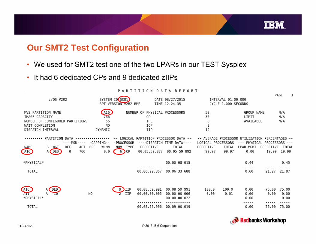
© 2015 IBM CorporationITSO-165
Our SMT2 Test Configuration
• We used for SMT2 test one of the two LPARs in our TEST Sysplex
• It had 6 dedicated CPs and 9 dedicated zIIPs
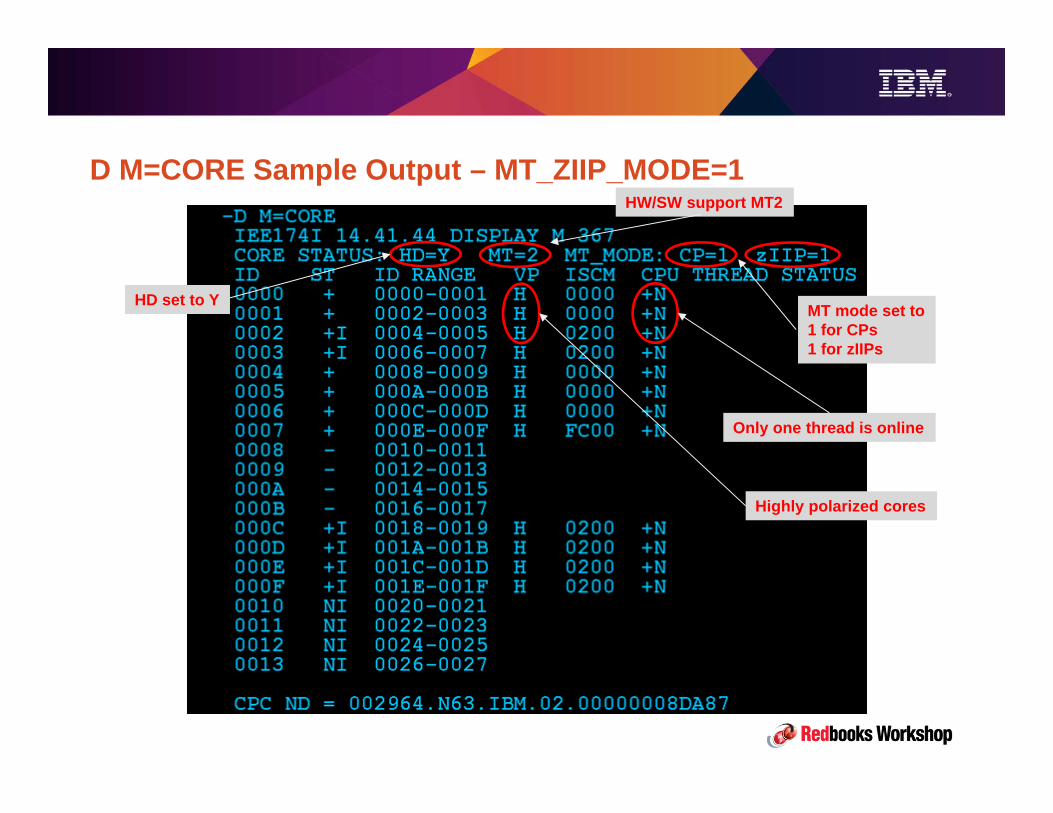
© 2015 IBM CorporationITSO-166
D M=CORE Sample Output – MT_ZIIP_MODE=1
HD set to Y
HW/SW support MT2
MT mode set to1 for CPs 1 for zIIPs
Only one thread is online
Highly polarized cores

© 2015 IBM CorporationITSO-167
Checking IEAOPT settings via RMF III

© 2015 IBM CorporationITSO-168
Switching to MT_ZIIP_MODE=2
We dynamically switched to SMT2 for zIIPS changing a IEAOPTxx option ..
.. and issuing a SET OPT command ..
Let us see the effect of this change ..
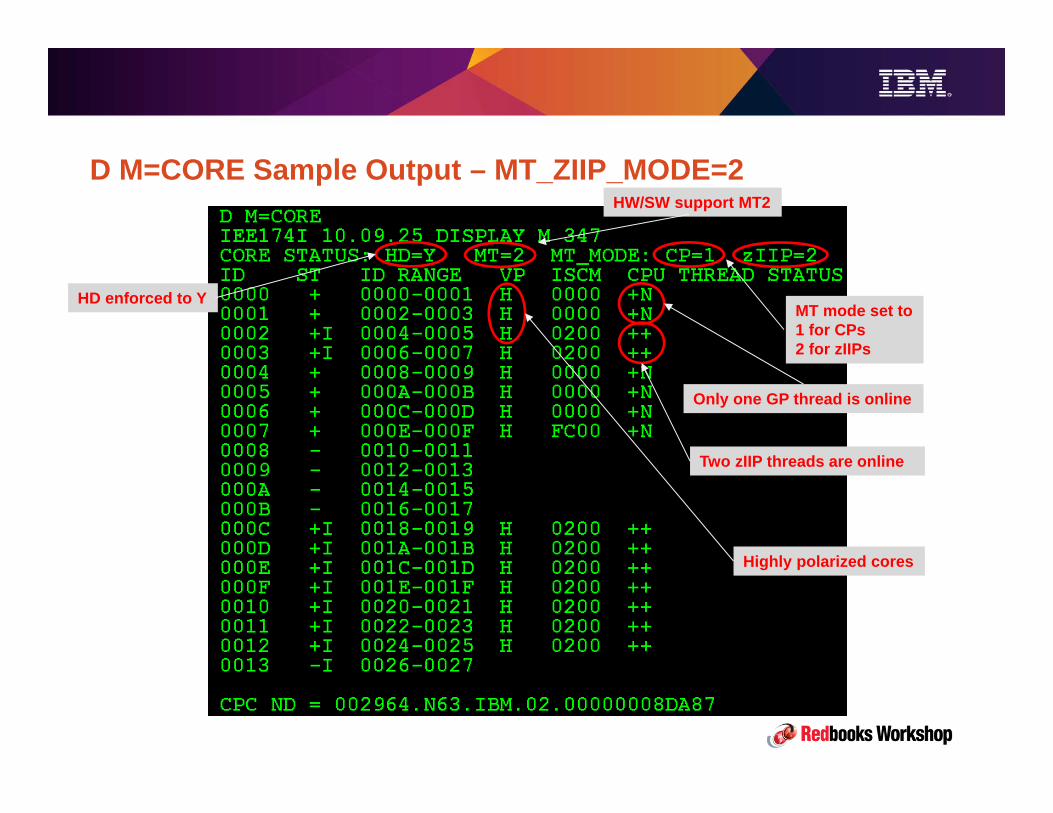
© 2015 IBM CorporationITSO-169
D M=CORE Sample Output – MT_ZIIP_MODE=2
HD enforced to Y
HW/SW support MT2
MT mode set to1 for CPs 2 for zIIPs
Only one GP thread is online
Highly polarized cores
Two zIIP threads are online

© 2015 IBM CorporationITSO-170
We dynamically switched back to SMT1 removing the IEAOPTxx option ..
.. and issuing a SET OPT command ..
Switching back to MT_ZIIP_MODE=1

© 2015 IBM CorporationITSO-171
z/OS SMT Performance Metrics
The introduction of SMT required new metrics and changes to existing ones
• CPU metric data can now be on core or thread level granularity
• z/OS charges CPU time consumed by work units (TCBs, SRBs) in terms of MT-1 equivalent time.
• MT-1 equivalent time is the [CPU] time it would have taken to run the same work in MT-1 mode
• This allows consistent accounting of processor usage despite the variability of the gain you can obtain
enabling SMT-2 on zIIP processors.
• New metrics are derived from LPAR level counters made available by the Hardware Instrumentation
Services .
HIS STC doesn’t need to be active, but you need to enable hardware counters collection via HMC

© 2015 IBM CorporationITSO-172
RMF CPU Activity Report – New format for PROCVIEW CORE• When running in PROCVIEW CORE mode the CPU Activity section reports on logical core
and logical processor activity. It provides a set of calculations which granularity depends on
whether multithreading is disabled or enabled.
• If multithreading is disabled for a processor type, all calculations are at logical processor
granularity. If multithreading is enabled for a processor type, some calculations are
provided at logical core granularity and some are provided at logical processor (thread)
granularity.
• The CPU Activity section displays exactly one report line per thread showing all calculations
at logical processor granularity
• Calculations that are provided at core granularity are only shown in the same report line
that shows the core id in the CPU NUM field and which represents the first thread of a core
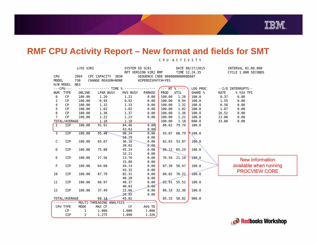
© 2015 IBM CorporationITSO-173
RMF CPU Activity Report – New format and fields for SMT
New Information available when running
PROCVIEW CORE

© 2015 IBM CorporationITSO-174
RMF CPU Activity Report – New fields for SMT• MT % PROD – Multi Threading Productivity
– The percentage of the maximum core capacity that was used in the reporting interval while the logical core was
dispatched to physical hardware. When MT % PROD equals 100% and the LOADxx PROCVIEW CORE parameter
is in effect, all threads on the core are executing work and all core resources are being used. If MT % PROD is less
than 100%, the core resources were dispatched to physical hardware but one or more threads on a logical core were
in a wait because they had no work to run (% Used MT-2 Core Capacity during Core Busy Time).
• MT % UTIL – The percentage of the maximum core capacity that was used in the reporting interval (% Used MT-2 Core Capacity
during Measurement Interval).91.91 * 86.82 / 100 = 79.79

© 2015 IBM CorporationITSO-175
RMF CPU Activity Report – New fields for SMT• Multithreading Capacity Factor for a processor type (CF).
– It represents the ratio of the amount of work that has been accomplished within this reporting interval to the amount
of work that would have been accomplished with multithreading disabled. MT1 CF = 1.0 (100%). So this is the actual
relative capacity we got with our workload during this measurement interval (Actual MT-2 Efficiency).
• Multithreading maximum Capacity Factor for a processor type (MAX CF). – It represents the ratio of the maximum amount of work that can be accomplished using all active threads to the
amount of work that would have been accomplished within this reporting interval when multithreading was disabled.
MT1 CF = 1.0 (100%). This is the relative capacity we could theoretically achieve with our workload with all the
threads in each core fully busy (Estimated max MT-2 Efficiency).
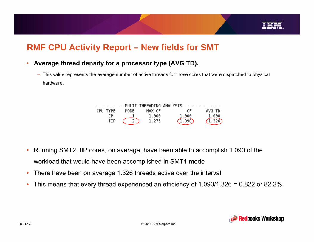
© 2015 IBM CorporationITSO-176
RMF CPU Activity Report – New fields for SMT• Average thread density for a processor type (AVG TD).
– This value represents the average number of active threads for those cores that were dispatched to physical
hardware.
• Running SMT2, IIP cores, on average, have been able to accomplish 1.090 of the
workload that would have been accomplished in SMT1 mode
• There have been on average 1.326 threads active over the interval
• This means that every thread experienced an efficiency of 1.090/1.326 = 0.822 or 82.2%
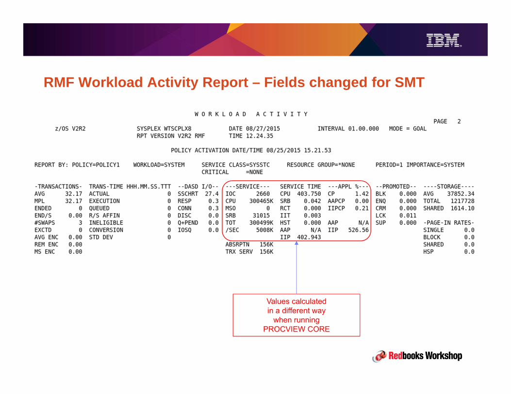
© 2015 IBM CorporationITSO-177
RMF Workload Activity Report – Fields changed for SMT
Values calculated in a different way
when running PROCVIEW CORE

© 2015 IBM CorporationITSO-178
RMF Workload Activity Report – Fields changed for SMT
• When running MT-2 Service Times and Service Units charged to workloads are MT-1
equivalent (CPU time / service units that would have been used in MT-1 mode). They are
normalized using actual Capacity Factor.
New Service Times and Service Units calculation also applies to relevant SMF30 fields
402.943 / 0.822 = 490.198would be the actual
IIP Service Time

© 2015 IBM CorporationITSO-179
RMF Workload Activity Report – Fields changed for SMT
• When running MT-2 APPL% represents the percentage of maximum core capacity used
by the workload. They are normalized using maximum Capacity Factor (mCF).
Note that mCF can change over time affecting comparison of APPL% values
402.943 / 60.000 = 671.57%The good old way to calculate IIP APPL%
doesn’t work for SMT2

© 2015 IBM CorporationITSO-180
RMF CPU Activity Report – SMT1 Example
74.78 * 9 zIIPS = 673.02 zIIP%
With WC=N when the only thread enters the WAIT state the CORE
is undispatched by PR/SM so LPAR BUSY% = UTIL%

© 2015 IBM CorporationITSO-181
RMF Workload Activity Report – SMT1 Example
(401.294 / 59.999) / 1.000 = 668.83%
In SMT1 mode Capture Ratio can be calculated as APPL% divided by LPAR Busy%
For zIIPs it is:
668.83 / 673.02 = 99.38%
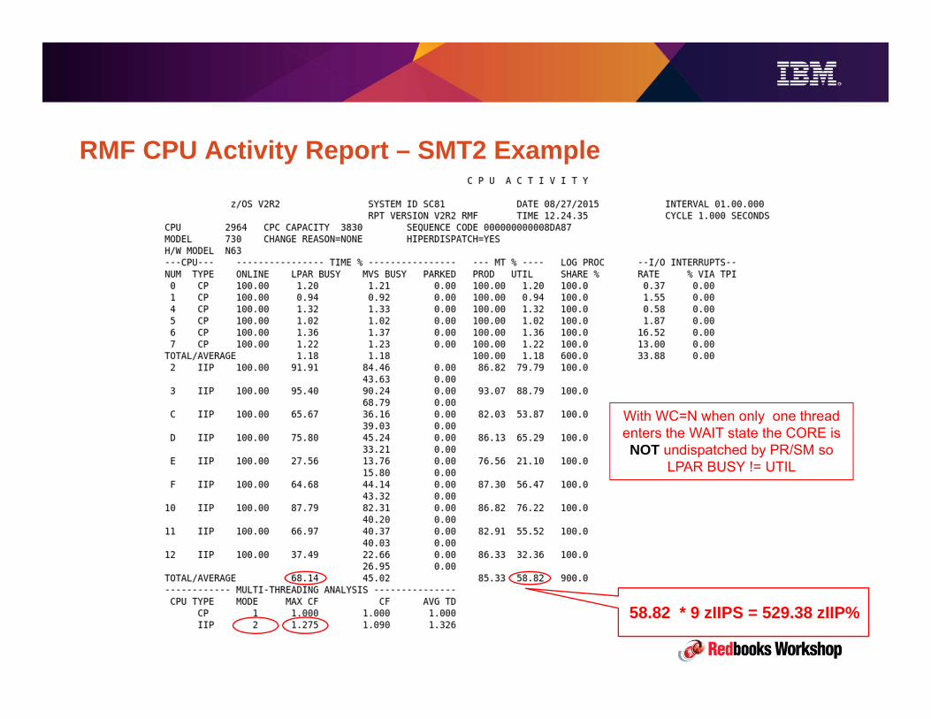
© 2015 IBM CorporationITSO-182
RMF CPU Activity Report – SMT2 Example
58.82 * 9 zIIPS = 529.38 zIIP%
With WC=N when only one thread enters the WAIT state the CORE is NOT undispatched by PR/SM so
LPAR BUSY != UTIL

© 2015 IBM CorporationITSO-183
RMF Workload Activity Report – SMT2 Example
(402.943 / 60.000) / 1.275 = 526.56%
In SMT2 mode Capture Ratio must be calculated as APPL% divided by MT UTIL%
For zIIPs it is:
526.56 / 529.38 = 99.46%
© 2015 IBM CorporationITSO-184
RMF Monitor III – New panels format for PROCVIEW CORE
• RMF monitor III has also been changed to report new information relevant when
running in PROCVIEW CORE mode.
• The following few slides have snapshots of some z/OS 2.2 panels showing the
most important changes.

© 2015 IBM CorporationITSO-185
RMF III CPC Capacity – PROCVIEW CPU

© 2015 IBM CorporationITSO-186
RMF III CPC Capacity – PROCVIEW CORE (SMT1)
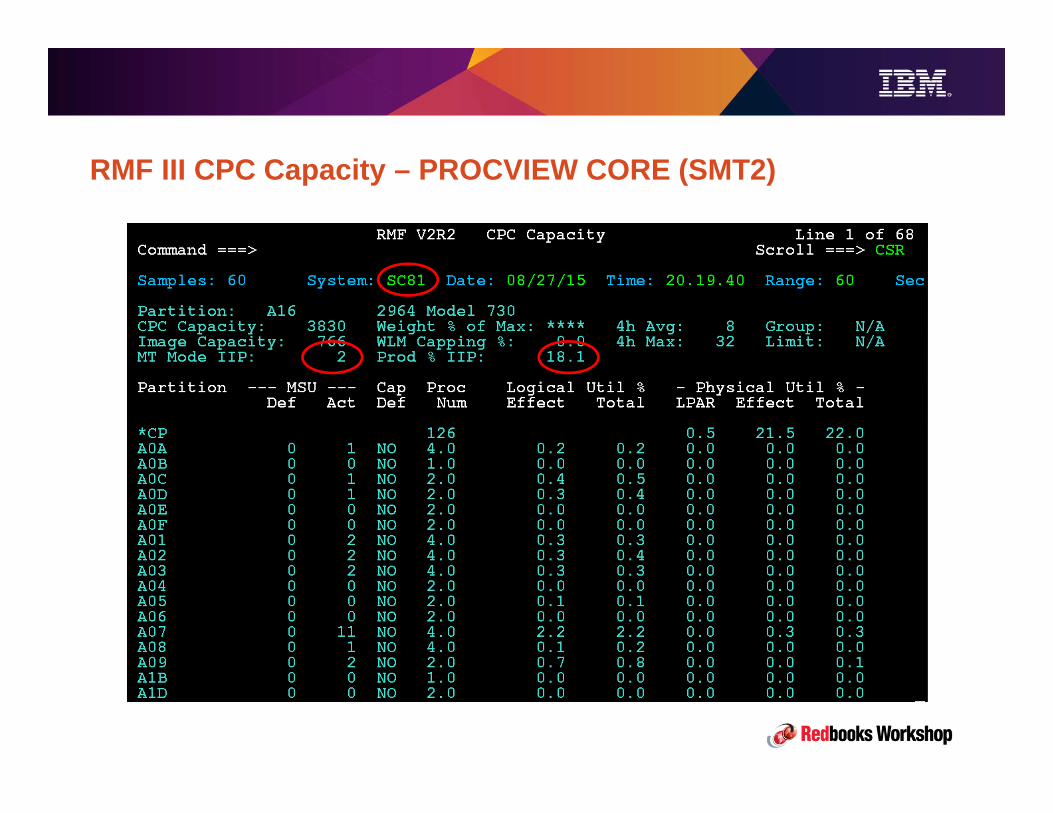
© 2015 IBM CorporationITSO-187
RMF III CPC Capacity – PROCVIEW CORE (SMT2)
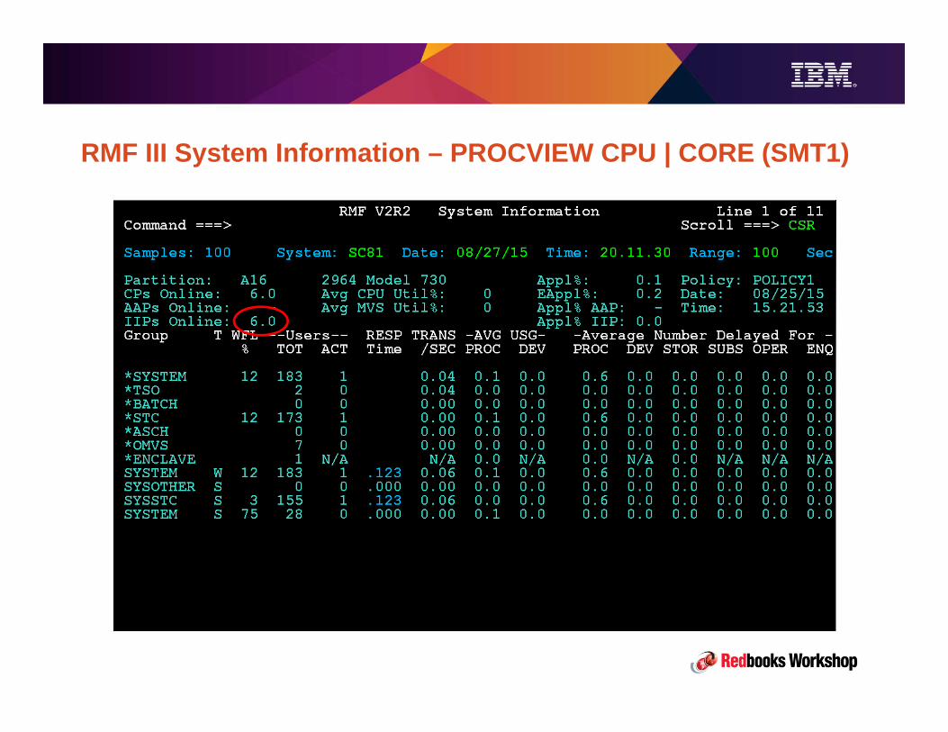
© 2015 IBM CorporationITSO-188
RMF III System Information – PROCVIEW CPU | CORE (SMT1)

© 2015 IBM CorporationITSO-189
RMF III System Information – PROCVIEW CORE (SMT2)
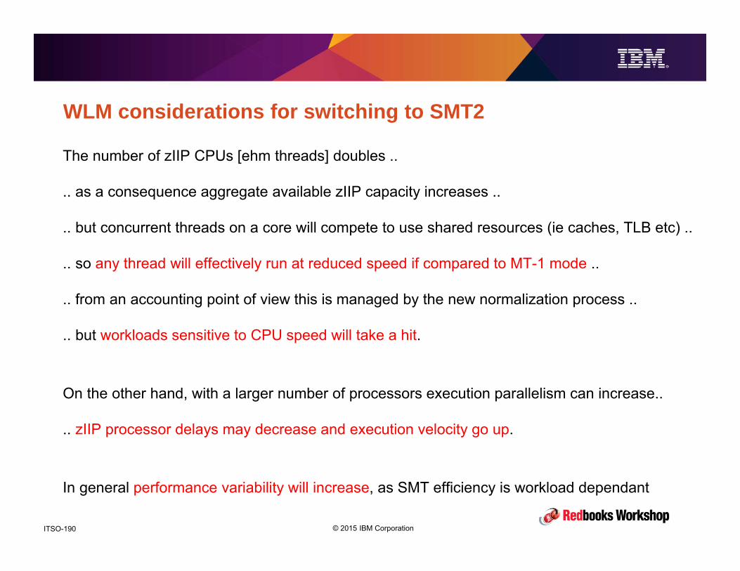
© 2015 IBM CorporationITSO-190
WLM considerations for switching to SMT2
The number of zIIP CPUs [ehm threads] doubles ..
.. as a consequence aggregate available zIIP capacity increases ..
.. but concurrent threads on a core will compete to use shared resources (ie caches, TLB etc) ..
.. so any thread will effectively run at reduced speed if compared to MT-1 mode ..
.. from an accounting point of view this is managed by the new normalization process ..
.. but workloads sensitive to CPU speed will take a hit.
On the other hand, with a larger number of processors execution parallelism can increase..
.. zIIP processor delays may decrease and execution velocity go up.
In general performance variability will increase, as SMT efficiency is workload dependant

© 2015 IBM CorporationITSO-191
Z13 SMT Summary
• z13 is the first System z Processor to support SMT
– z13 supports 2 threads per core on IFLs and zIIPs only
• SMT enables continued scaling of per-processor capacity
– SMT Increases per-core and system throughput versus single thread design
– but in SMT mode threads run at reduced speed if compared to single thread mode
• Different workloads and different workload mixes will exhibit different throughput
gains and thread slow downs.
• For most customers the choice between enabling SMT2 or adding more zIIP
engines will mainly be driven by financial considerations
© 2015 IBM CorporationITSO-192
z13 Parallel Sysplex CouplingPerformance and Availability

© 2015 IBM CorporationITSO-193
Introduction
• One of the most notable changes in z13 is that the CPC has been redesigned to package
processors in drawers, compared to books as they were in earlier machines.
• z13 supports two distinct connectivity infrastructures: The one based on Infiniband
technology, to connect legacy I/O, and the one based on PCIe Gen3 technology for newer
adapters.
• Each z13 CPC drawer provides connectors to support PCIe I/O drawers (through PCIe
fanout hubs), I/O drawers through InfiniBand features, and coupling links to other CPCs.
• Following the trend of implementing new adapters using PCIe, z13 offers a new short
reach Coupling Link technology called ICA-SR based on PCIe Gen3 technology.
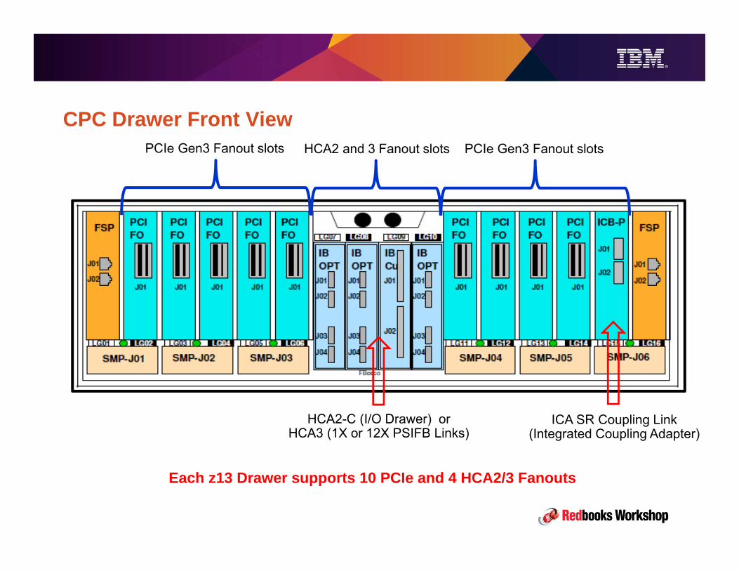
© 2015 IBM CorporationITSO-194
CPC Drawer Front ViewHCA2 and 3 Fanout slotsPCIe Gen3 Fanout slots PCIe Gen3 Fanout slots
ICA SR Coupling Link(Integrated Coupling Adapter)
HCA2-C (I/O Drawer) or HCA3 (1X or 12X PSIFB Links)
Each z13 Drawer supports 10 PCIe and 4 HCA2/3 Fanouts
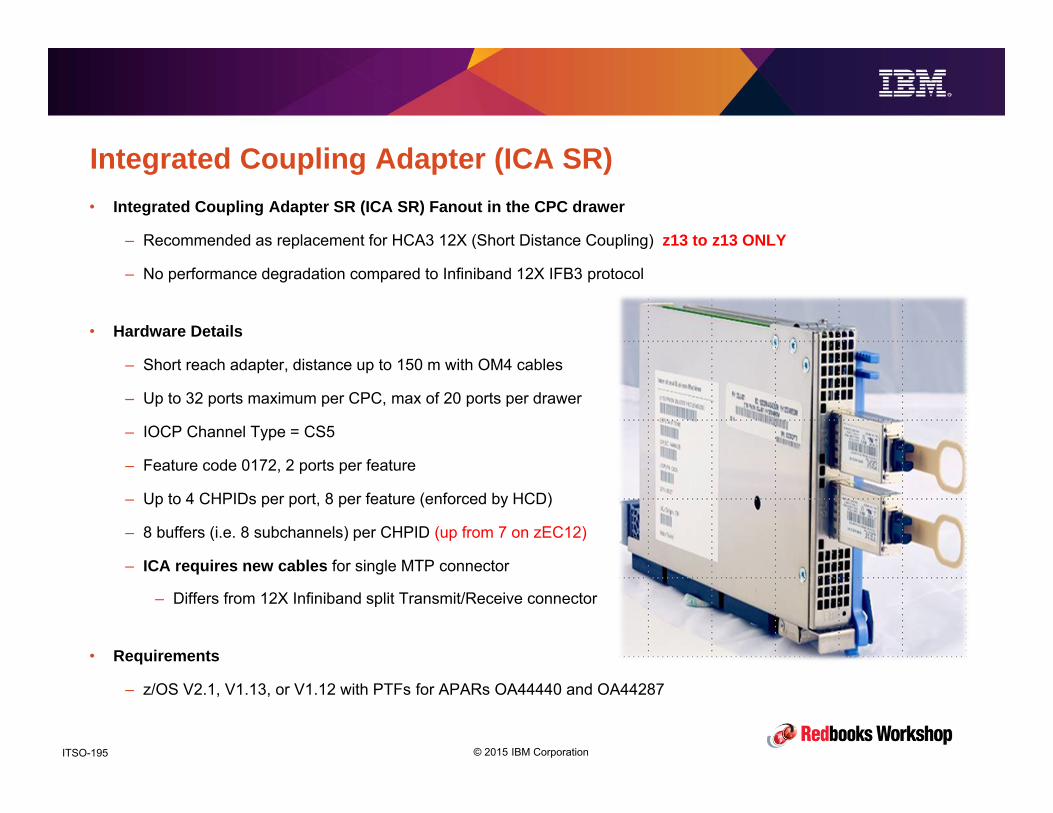
© 2015 IBM CorporationITSO-195
Integrated Coupling Adapter (ICA SR)• Integrated Coupling Adapter SR (ICA SR) Fanout in the CPC drawer
– Recommended as replacement for HCA3 12X (Short Distance Coupling) z13 to z13 ONLY
– No performance degradation compared to Infiniband 12X IFB3 protocol
• Hardware Details
– Short reach adapter, distance up to 150 m with OM4 cables
– Up to 32 ports maximum per CPC, max of 20 ports per drawer
– IOCP Channel Type = CS5
– Feature code 0172, 2 ports per feature
– Up to 4 CHPIDs per port, 8 per feature (enforced by HCD)
– 8 buffers (i.e. 8 subchannels) per CHPID (up from 7 on zEC12)
– ICA requires new cables for single MTP connector
– Differs from 12X Infiniband split Transmit/Receive connector
• Requirements
– z/OS V2.1, V1.13, or V1.12 with PTFs for APARs OA44440 and OA44287

© 2015 IBM CorporationITSO-196
ICA SR – IOCP Example
CHPID PATH=(CSS(1),88),SHARED,PARTITION=((A1C,A11,A16),(=)), *CPATH=(CSS(1),9C),CSYSTEM=SCZP501,AID=27,PORT=1,TYPE=CS5
CHPID PATH=(CSS(1),89),SHARED,PARTITION=((A1C,A11,A16),(=)), *CPATH=(CSS(1),9D),CSYSTEM=SCZP501,AID=27,PORT=1,TYPE=CS5
CHPID PATH=(CSS(1),98),SHARED,PARTITION=((A1C,A11,A16),(=)), *CPATH=(CSS(1),8C),CSYSTEM=SCZP501,AID=27,PORT=2,TYPE=CS5
CHPID PATH=(CSS(1),99),SHARED,PARTITION=((A1C,A11,A16),(=)), *CPATH=(CSS(1),8D),CSYSTEM=SCZP501,AID=27,PORT=2,TYPE=CS5
CHPID PATH=(CSS(1),8C),SHARED,PARTITION=((A1F,A11,A16),(=)), *CPATH=(CSS(1),98),CSYSTEM=SCZP501,AID=34,PORT=1,TYPE=CS5
CHPID PATH=(CSS(1),8D),SHARED,PARTITION=((A1F,A11,A16),(=)), *CPATH=(CSS(1),99),CSYSTEM=SCZP501,AID=34,PORT=1,TYPE=CS5
CHPID PATH=(CSS(1),9C),SHARED,PARTITION=((A1F,A11,A16),(=)), *CPATH=(CSS(1),88),CSYSTEM=SCZP501,AID=34,PORT=2,TYPE=CS5
CHPID PATH=(CSS(1),9D),SHARED,PARTITION=((A1F,A11,A16),(=)), *CPATH=(CSS(1),89),CSYSTEM=SCZP501,AID=34,PORT=2,TYPE=CS5
CNTLUNIT CUNUMBR=FFE7,PATH=((CSS(1),88,98,89,99)),UNIT=CFPIODEVICE ADDRESS=(FF49,008),CUNUMBR=(FFE7),UNIT=CFPIODEVICE ADDRESS=(FFAE,008),CUNUMBR=(FFE7),UNIT=CFPIODEVICE ADDRESS=(FFB6,008),CUNUMBR=(FFE7),UNIT=CFPIODEVICE ADDRESS=(FFD5,008),CUNUMBR=(FFE7),UNIT=CFP
CNTLUNIT CUNUMBR=FFED,PATH=((CSS(1),9C,8C,9D,8D)),UNIT=CFPIODEVICE ADDRESS=(FF96,008),CUNUMBR=(FFED),UNIT=CFPIODEVICE ADDRESS=(FFA6,008),CUNUMBR=(FFED),UNIT=CFPIODEVICE ADDRESS=(FFBE,008),CUNUMBR=(FFED),UNIT=CFPIODEVICE ADDRESS=(FFC6,008),CUNUMBR=(FFED),UNIT=CFP
When a production IODF is built, all CS5 channel paths have to be connected
2 channels per port
8 subchannels per CHPID
Single z13 configuration – 2 x 4 logical channels

© 2015 IBM CorporationITSO-197
ICA SR– D CF command output
D CF IXL150I 10.39.33 DISPLAY CF 051 COUPLING FACILITY 002964.IBM.02.00000008DA87
PARTITION: 1F CPCID: 00 LP NAME: A1F CPC NAME: SCZP501 CONTROL UNIT ID: FFE7
NAMED CF8A
PATH PHYSICAL LOGICAL CHANNEL TYPE AID PORT 88 / 050D ONLINE ONLINE CS5 8X-PCIE3 0027 01 89 / 050E ONLINE ONLINE CS5 8X-PCIE3 0027 01 98 / 0512 ONLINE ONLINE CS5 8X-PCIE3 0027 02 99 / 0513 ONLINE ONLINE CS5 8X-PCIE3 0027 02 C6 ONLINE ONLINE ICP N/A N/AC7 ONLINE ONLINE ICP N/A N/A

© 2015 IBM CorporationITSO-198
ICA SR– RMF Monitor III Status Display

© 2015 IBM CorporationITSO-199
ICA SR– RMF Post Processor Subchannel Activity
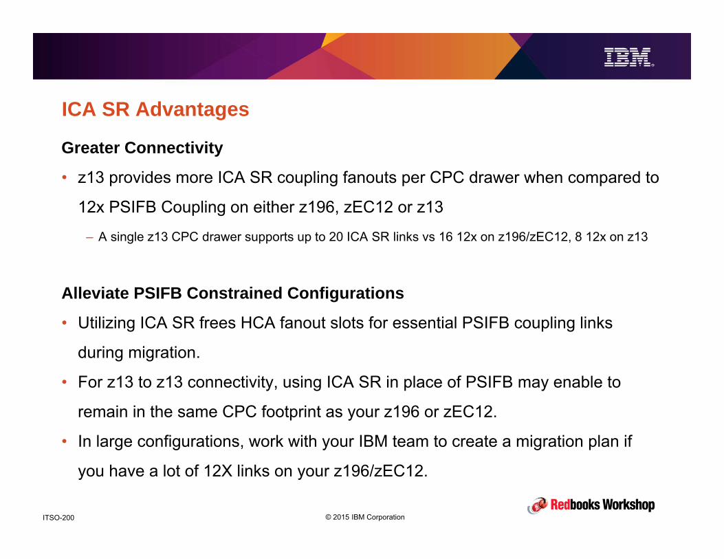
© 2015 IBM CorporationITSO-200
ICA SR Advantages
Greater Connectivity
• z13 provides more ICA SR coupling fanouts per CPC drawer when compared to
12x PSIFB Coupling on either z196, zEC12 or z13
– A single z13 CPC drawer supports up to 20 ICA SR links vs 16 12x on z196/zEC12, 8 12x on z13
Alleviate PSIFB Constrained Configurations
• Utilizing ICA SR frees HCA fanout slots for essential PSIFB coupling links
during migration.
• For z13 to z13 connectivity, using ICA SR in place of PSIFB may enable to
remain in the same CPC footprint as your z196 or zEC12.
• In large configurations, work with your IBM team to create a migration plan if
you have a lot of 12X links on your z196/zEC12.
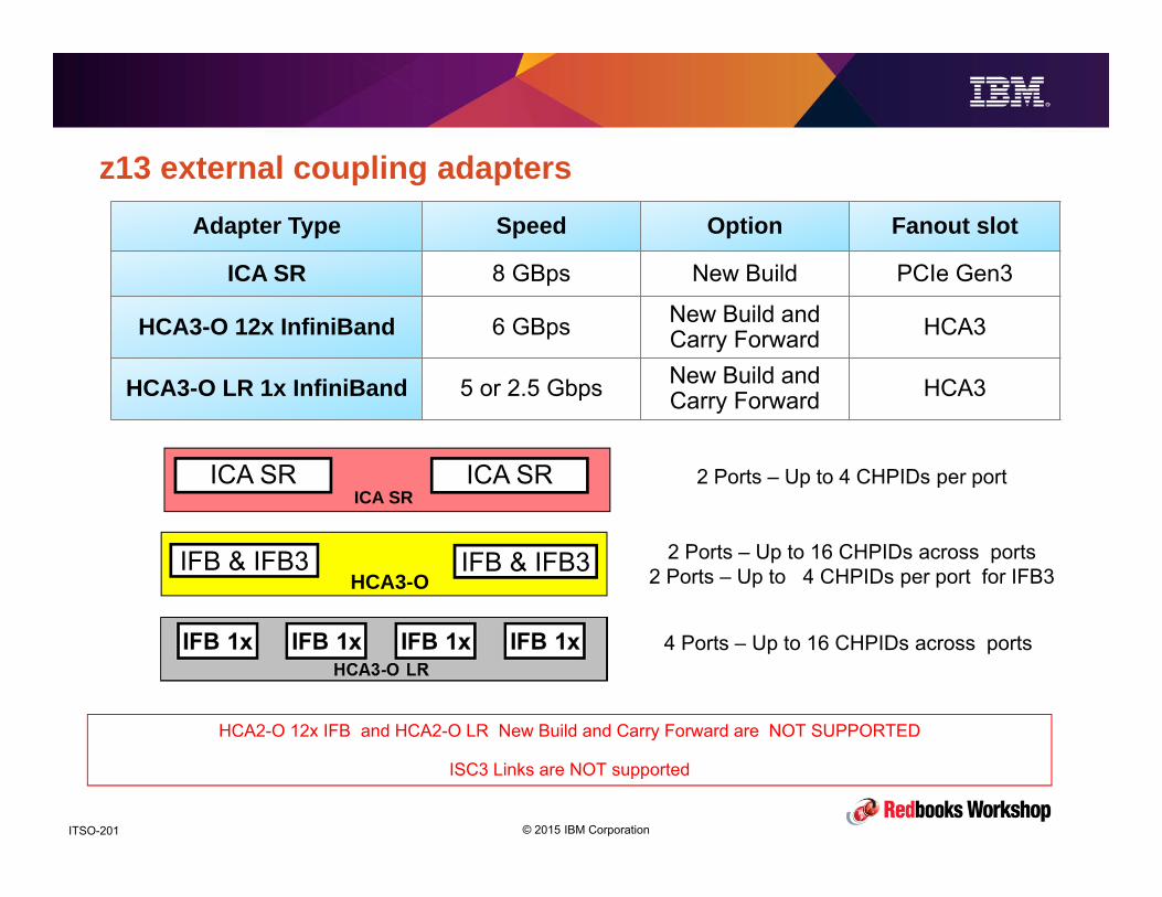
© 2015 IBM CorporationITSO-201
z13 external coupling adaptersAdapter Type Speed Option Fanout slot
ICA SR 8 GBps New Build PCIe Gen3
HCA3-O 12x InfiniBand 6 GBps New Build and Carry Forward HCA3
HCA3-O LR 1x InfiniBand 5 or 2.5 Gbps New Build and Carry Forward HCA3
ICA SRICA SR ICA SR
HCA3-OIFB & IFB3 IFB & IFB3
2 Ports – Up to 4 CHPIDs per port
2 Ports – Up to 16 CHPIDs across ports2 Ports – Up to 4 CHPIDs per port for IFB3
4 Ports – Up to 16 CHPIDs across ports
HCA2-O 12x IFB and HCA2-O LR New Build and Carry Forward are NOT SUPPORTED
ISC3 Links are NOT supported
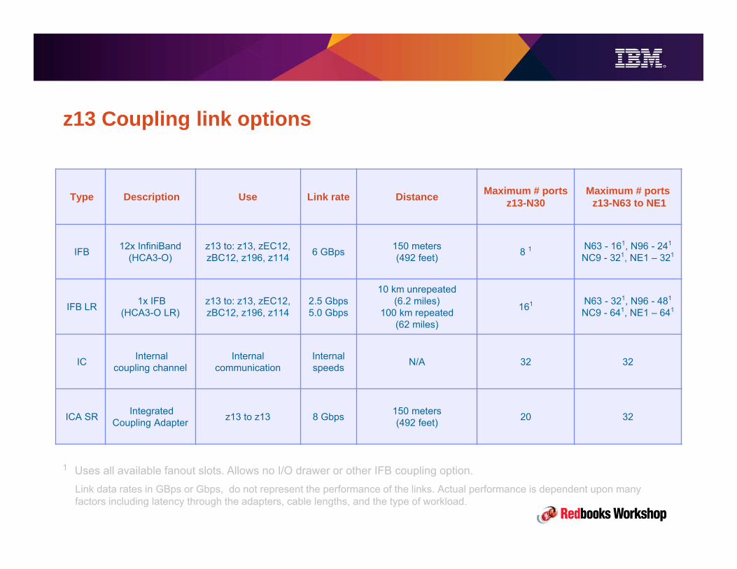
© 2015 IBM CorporationITSO-202
z13 Coupling link options
Type Description Use Link rate Distance Maximum # portsz13-N30
Maximum # portsz13-N63 to NE1
IFB 12x InfiniBand (HCA3-O)
z13 to: z13, zEC12, zBC12, z196, z114 6 GBps 150 meters
(492 feet) 8 1 N63 - 161, N96 - 241
NC9 - 321, NE1 – 321
IFB LR 1x IFB (HCA3-O LR)
z13 to: z13, zEC12, zBC12, z196, z114
2.5 Gbps5.0 Gbps
10 km unrepeated (6.2 miles)
100 km repeated (62 miles)
161 N63 - 321, N96 - 481
NC9 - 641, NE1 – 641
IC Internal coupling channel
Internal communication
Internal speeds N/A 32 32
ICA SR Integrated Coupling Adapter z13 to z13 8 Gbps 150 meters
(492 feet) 20 32
1 Uses all available fanout slots. Allows no I/O drawer or other IFB coupling option.Link data rates in GBps or Gbps, do not represent the performance of the links. Actual performance is dependent upon many factors including latency through the adapters, cable lengths, and the type of workload.

© 2015 IBM CorporationITSO-203
Coupling Technology versus Host Processor Speed
With z/OS 1.2 and above, synch-> asynch conversion caps values in the table at about 18%IC links scale with the speed of the host technology and would provide an 8% effect in each case
Host effect with primary application involved in data sharing Chart is based on 9 CF ops/Mi – may be scaled linearly for other rates
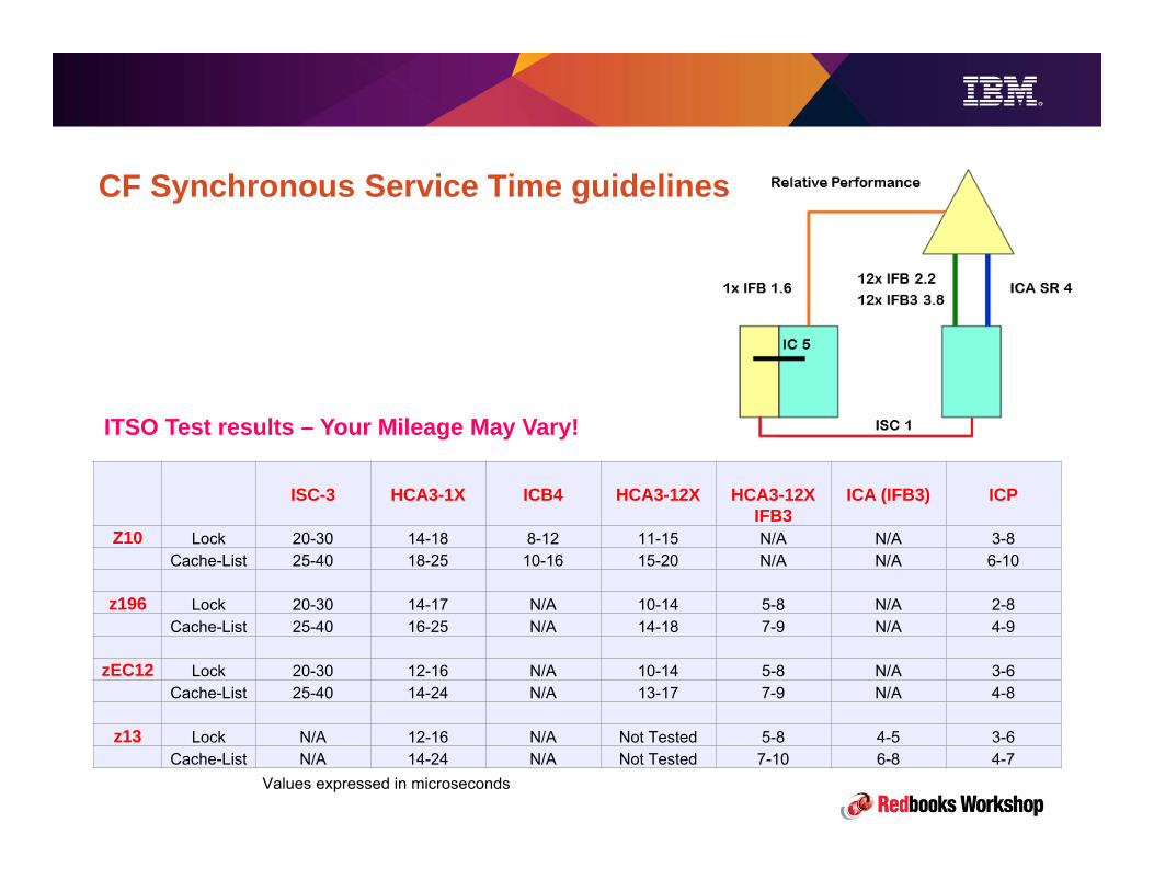
© 2015 IBM CorporationITSO-204
CF Synchronous Service Time guidelines
ISC-3 HCA3-1X ICB4 HCA3-12X HCA3-12X IFB3
ICA (IFB3) ICP
Z10 Lock 20-30 14-18 8-12 11-15 N/A N/A 3-8Cache-List 25-40 18-25 10-16 15-20 N/A N/A 6-10
z196 Lock 20-30 14-17 N/A 10-14 5-8 N/A 2-8Cache-List 25-40 16-25 N/A 14-18 7-9 N/A 4-9
zEC12 Lock 20-30 12-16 N/A 10-14 5-8 N/A 3-6Cache-List 25-40 14-24 N/A 13-17 7-9 N/A 4-8
z13 Lock N/A 12-16 N/A Not Tested 5-8 4-5 3-6Cache-List N/A 14-24 N/A Not Tested 7-10 6-8 4-7
Values expressed in microseconds
ITSO Test results – Your Mileage May Vary!
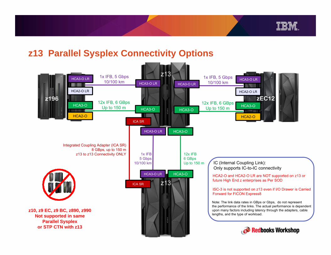
© 2015 IBM CorporationITSO-205
z13 Parallel Sysplex Connectivity Options
HCA3-O LRHCA3-O LR
1x IFB, 5 Gbps10/100 km
HCA3-O HCA3-O
12x IFB, 6 GBpsUp to 150 m
HCA3-O LRHCA3-O LR1x IFB, 5 Gbps
10/100 km
HCA3-O HCA3-O
12x IFB, 6 GBpsUp to 150 m
HCA3-O LR HCA3-O
ICA SR
ICA SR
12x IFB 6 GBpsUp to 150 m
1x IFB5 Gbps
10/100 km
Integrated Coupling Adapter (ICA SR)8 GBps, up to 150 m
z13 to z13 Connectivity ONLY
HCA2-O LR HCA2-O LR
HCA2-O HCA2-O
HCA3-O LR HCA3-O
IC (Internal Coupling Link): Only supports IC-to-IC connectivity
HCA2-O and HCA2-O LR are NOT supported on z13 or future High End z enterprises as Per SOD
ISC-3 is not supported on z13 even if I/O Drawer is Carried Forward for FICON Express8
Note: The link data rates in GBps or Gbps, do not representthe performance of the links. The actual performance is dependent upon many factors including latency through the adapters, cable lengths, and the type of workload.
z10, z9 EC, z9 BC, z890, z990 Not supported in same
Parallel Sysplex or STP CTN with z13
z196 zEC12
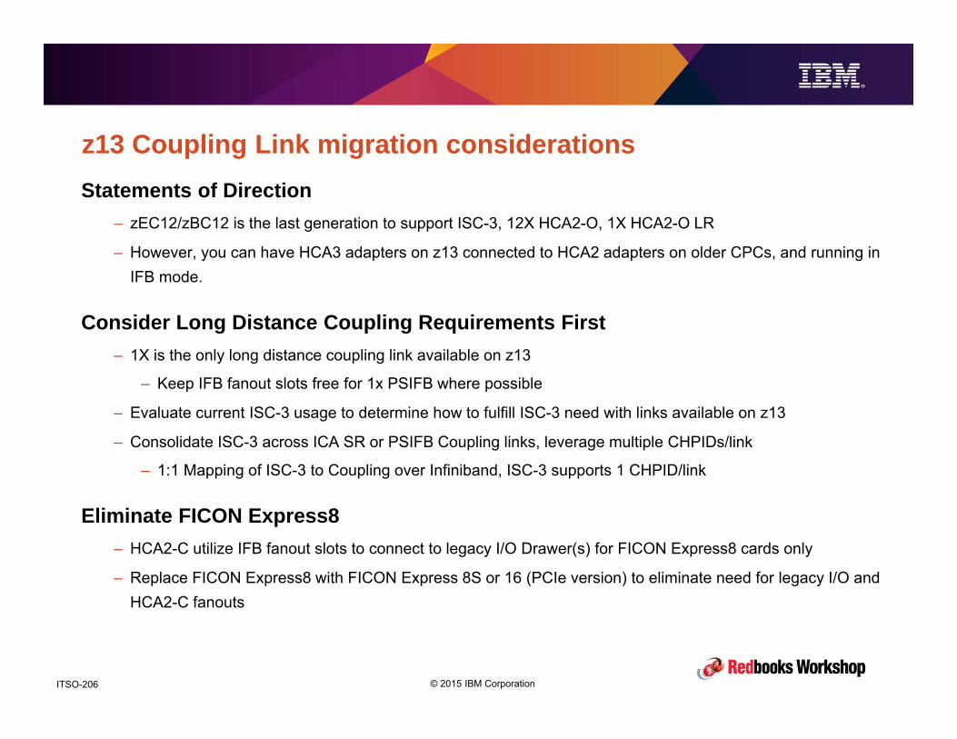
© 2015 IBM CorporationITSO-206
z13 Coupling Link migration considerationsStatements of Direction
– zEC12/zBC12 is the last generation to support ISC-3, 12X HCA2-O, 1X HCA2-O LR
– However, you can have HCA3 adapters on z13 connected to HCA2 adapters on older CPCs, and running in IFB mode.
Consider Long Distance Coupling Requirements First– 1X is the only long distance coupling link available on z13
– Keep IFB fanout slots free for 1x PSIFB where possible
– Evaluate current ISC-3 usage to determine how to fulfill ISC-3 need with links available on z13
– Consolidate ISC-3 across ICA SR or PSIFB Coupling links, leverage multiple CHPIDs/link
– 1:1 Mapping of ISC-3 to Coupling over Infiniband, ISC-3 supports 1 CHPID/link
Eliminate FICON Express8– HCA2-C utilize IFB fanout slots to connect to legacy I/O Drawer(s) for FICON Express8 cards only
– Replace FICON Express8 with FICON Express 8S or 16 (PCIe version) to eliminate need for legacy I/O and HCA2-C fanouts
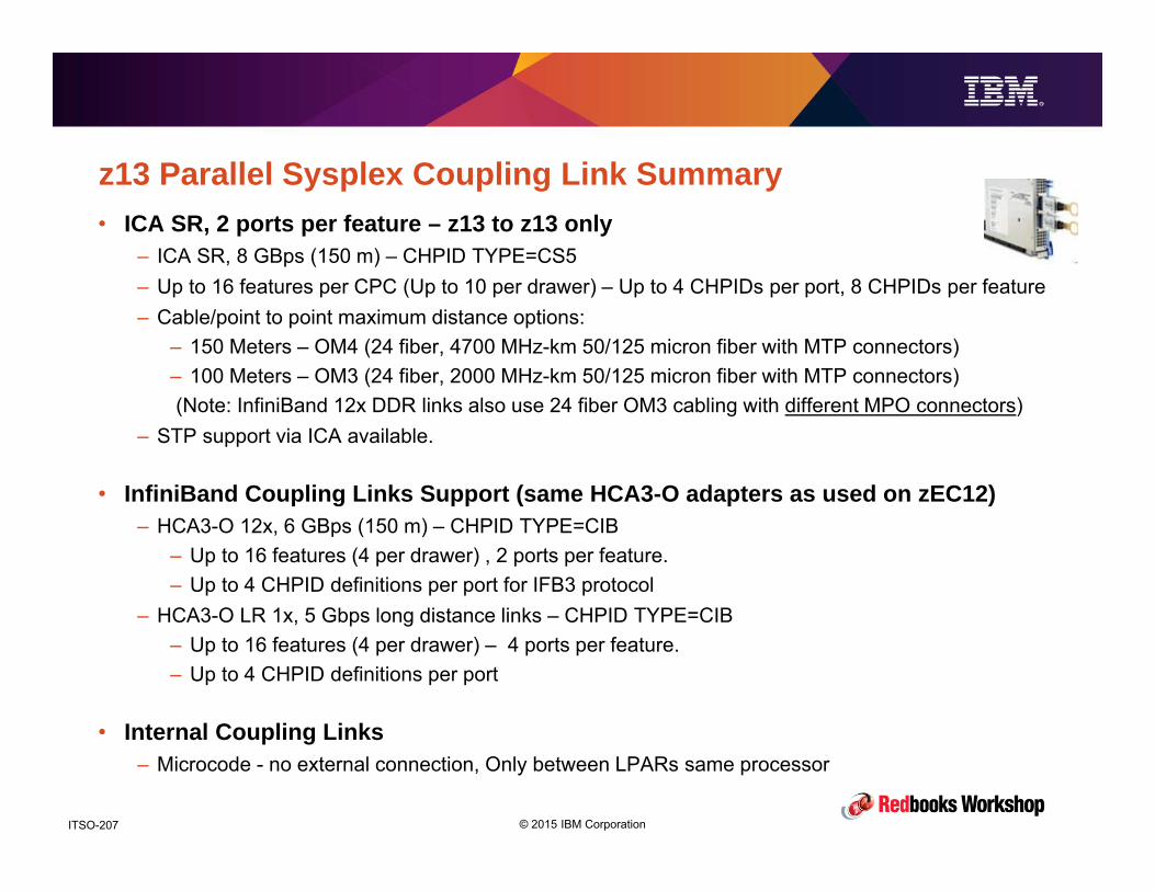
© 2015 IBM CorporationITSO-207
z13 Parallel Sysplex Coupling Link Summary• ICA SR, 2 ports per feature – z13 to z13 only
– ICA SR, 8 GBps (150 m) – CHPID TYPE=CS5– Up to 16 features per CPC (Up to 10 per drawer) – Up to 4 CHPIDs per port, 8 CHPIDs per feature– Cable/point to point maximum distance options:
– 150 Meters – OM4 (24 fiber, 4700 MHz-km 50/125 micron fiber with MTP connectors)– 100 Meters – OM3 (24 fiber, 2000 MHz-km 50/125 micron fiber with MTP connectors)(Note: InfiniBand 12x DDR links also use 24 fiber OM3 cabling with different MPO connectors)
– STP support via ICA available.
• InfiniBand Coupling Links Support (same HCA3-O adapters as used on zEC12)– HCA3-O 12x, 6 GBps (150 m) – CHPID TYPE=CIB
– Up to 16 features (4 per drawer) , 2 ports per feature. – Up to 4 CHPID definitions per port for IFB3 protocol
– HCA3-O LR 1x, 5 Gbps long distance links – CHPID TYPE=CIB– Up to 16 features (4 per drawer) – 4 ports per feature. – Up to 4 CHPID definitions per port
• Internal Coupling Links– Microcode - no external connection, Only between LPARs same processor

© 2015 IBM CorporationITSO-208
z13 CFCC Level 20 and STP
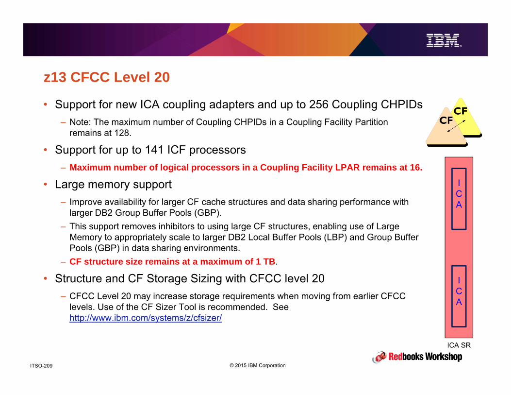
© 2015 IBM CorporationITSO-209
z13 CFCC Level 20
• Support for new ICA coupling adapters and up to 256 Coupling CHPIDs– Note: The maximum number of Coupling CHPIDs in a Coupling Facility Partition
remains at 128.
• Support for up to 141 ICF processors– Maximum number of logical processors in a Coupling Facility LPAR remains at 16.
• Large memory support– Improve availability for larger CF cache structures and data sharing performance with
larger DB2 Group Buffer Pools (GBP). – This support removes inhibitors to using large CF structures, enabling use of Large
Memory to appropriately scale to larger DB2 Local Buffer Pools (LBP) and Group Buffer Pools (GBP) in data sharing environments.
– CF structure size remains at a maximum of 1 TB.
• Structure and CF Storage Sizing with CFCC level 20– CFCC Level 20 may increase storage requirements when moving from earlier CFCC
levels. Use of the CF Sizer Tool is recommended. See http://www.ibm.com/systems/z/cfsizer/
ICA
ICA
ICA SR

© 2015 IBM CorporationITSO-210
CFCC 20 Improvements for Large Cache Structure Detach
• Prior to CFCC LEVEL=20, detach processing required a scan of every active
entry and registration block in the structure
– The larger the structure, the longer the scan takes to complete
– Exploiter had to wait for scan to complete before deemed to be detached
– Attachment “slot” cannot be reused until detach completes
• With CFCC LEVEL=20, the detach completes “instantly”
– Attachment “slot” immediately released; exploiter can immediately (re)attach
– CF still scans structure to clean up artifacts associated with the attachment that are no longer valid
– The CF can distinguish between artifacts associated with the new instance of the attachment versus
those associated with the old instance
New algorithm allows faster restart times for data sharing subsystems

© 2015 IBM CorporationITSO-211
z13 STP - Removal of Mixed CTN Support
• z13 can not participate in a mixed Coordinated Timing Network (CTN)
– Fulfills Statement Of Direction
– N-2 machine is z196 which does not support ETR
– Simplifies the code base
– Provides flexibility for future systems
z13 z10z10
9037
Migrate to STP-Only configuration before installing the first z13
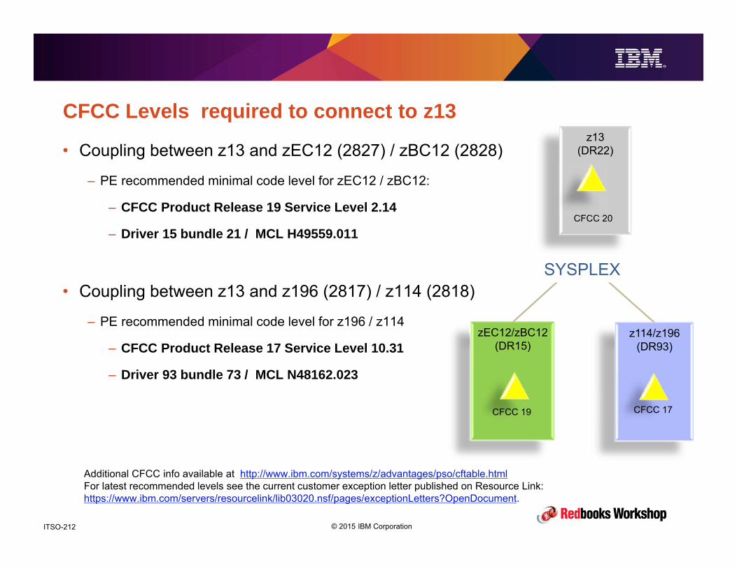
© 2015 IBM CorporationITSO-212
z13(DR22)
CFCC 20
CFCC Levels required to connect to z13
• Coupling between z13 and zEC12 (2827) / zBC12 (2828)
– PE recommended minimal code level for zEC12 / zBC12:
– CFCC Product Release 19 Service Level 2.14
– Driver 15 bundle 21 / MCL H49559.011
• Coupling between z13 and z196 (2817) / z114 (2818)
– PE recommended minimal code level for z196 / z114
– CFCC Product Release 17 Service Level 10.31
– Driver 93 bundle 73 / MCL N48162.023
zEC12/zBC12(DR15)
CFCC 19
z114/z196(DR93)
CFCC 17
SYSPLEXSYSPLEX
Additional CFCC info available at http://www.ibm.com/systems/z/advantages/pso/cftable.htmlFor latest recommended levels see the current customer exception letter published on Resource Link: https://www.ibm.com/servers/resourcelink/lib03020.nsf/pages/exceptionLetters?OpenDocument.

© 2015 IBM CorporationITSO-213
z13 Parallel Sysplex Coupling summary
• z13 with CFCC level 20 supports larger CF configurations– Up to 141 ICFs, up to 10TB memory
• z13 introduces new PCIe based short reach Coupling Link technology– If compared with PSIFB 12x IFB3 it provides similar performance and more connectivity per drawer
– Only available for z13 to z13 connections
• z13 has limited number of slots for Infiniband connectivity– They should be used to address long distance sysplex connectivity needs
– ISC3 and HCA2 InfiniBand adapters not available on z13
– Migration should be planned carefully
• REMINDER – anyone using Shared CF engines on zEC12 GA2 or later should
investigate use of Coupling Thin Interrupts

© 2015 IBM CorporationITSO-214
Erase on Scratch EnhancementsPerformance and Availability
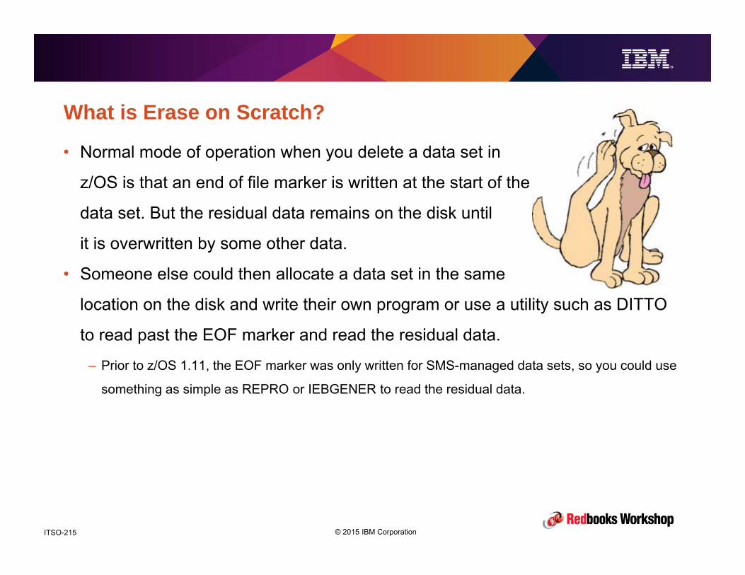
© 2015 IBM CorporationITSO-215
What is Erase on Scratch?
• Normal mode of operation when you delete a data set in
z/OS is that an end of file marker is written at the start of the
data set. But the residual data remains on the disk until
it is overwritten by some other data.
• Someone else could then allocate a data set in the same
location on the disk and write their own program or use a utility such as DITTO
to read past the EOF marker and read the residual data.
– Prior to z/OS 1.11, the EOF marker was only written for SMS-managed data sets, so you could use
something as simple as REPRO or IEBGENER to read the residual data.

© 2015 IBM CorporationITSO-216
What is Erase on Scratch?
• To protect against this exposure, RACF 1.7 delivered a capability called Erase-
On-Scratch. This (OPTIONALLY) changed the delete or partial release process
so that all freed-up tracks would be overwritten with zeroes. The delete or
partrel would not end until that processing had completed.
– This ensured that no one else could allocate a new data set until the contents of the old one had
been scratched.
– Initially the scratch processing was driven by DFP, 1 track at a time. So it was slow and consumed
LOTS of z/OS CPU time.
– And because it was part of the delete/partrel process, the delete or partrel would not end until the
scratch had finished. This could take a really REALLY long time, especially for large data sets.
– As a result, few customers used this capability.
– But this was prior to the days of hackers and highly publicized data breaches
© 2015 IBM CorporationITSO-217
How granular is Erase on Scratch?
• RACF provides 4 levels of control for EoS:
– SETR NOERASE EoS is disabled for all data sets.
– SETR ERASE Performs SCRATCH for data sets that specify ERASE in the DS profile.
– SETR ERASE (SECLEVEL(xx)) Performs SCRATCH for data sets with a SECLEVEL of ‘xx’ or higher.
– SETR ERASE(ALL) Performs SCRATCH for ALL data sets, including temp data sets.
• Presumably the level that you want to use will depend on the sensitivity of your
data and the impact of enabling EoS.
– But remember, the RACF control is associated with the data set, not the data. If you copy data from a
data set that is enabled for EoS to one that is not, the data will be exposed when the second data set
is deleted.
• So, what about performance?

© 2015 IBM CorporationITSO-218
EoS performance improvements
• The first significant performance improvement to EoS came in 1997 when RVA
DASD subsystems introduced a function called Deleted Data Space Release
(DDSR). DDSR dramatically improved the performance of scratch processing
because the scratch was now driven by the DASD control unit rather than by DFP.
– However EoS already had a reputation for bad performance, so no one cared.
• The next significant enhancement came in z/OS 2.1. A combination of code in
z/OS and new function in DASD subsystems (IBM 8100 and later) delivered the
ability to SCRATCH 255 tracks in a single request, rather than one track.
– Exception was PPRCed disks, because z/OS could not tell if the secondary DASD had the required
level of microcode.

© 2015 IBM CorporationITSO-219
EoS Performance enhancements

© 2015 IBM CorporationITSO-220
EoS Performance enhancements
© 2015 IBM CorporationITSO-221
EoS performance improvements
• APARs OA43693 and OA46511 (both CLOSED and for z/OS 2.1 only)
subsequently provided the ability for you to tell the operating system that the
secondary DASD subsystem in a PPRC pair does contain the required support.
This is controlled by a new EOSV2 parameter in the DEVSUPxx member.
Specifying EOSV2=YES indicates that the secondary subsystems support this
capability, meaning that DFSMS will erase up to 255 tracks at a time on PPRCed
disks, just as it does for simplex disks. Note that the default for EOSV2 is NO.
• Note that the basic enhancement in z/OS 2.1, increasing the number of tracks
from 1 to 255, happens automatically if the correct level of DASD microcode is
installed (see APAR OA46511 for information about the required microcode
levels).

© 2015 IBM CorporationITSO-222
EoS Pre-reqs
• RACF (presumably other security products have a similar capability).
• Check APAR OA46511 to make sure that you have the required DASD microcode
installed. If you have non-IBM DASD, check with your vendor.
• If you use PPRC, install the supporting PTFs and specify EOSV2=YES in your
DEVSUPxx member.
• For the latest performance improvements, should have z/OS V2.
– But the biggest performance improvements were delivered by the DASD enhancements
• Enable EoS using the SETR ERASExxxxx command.
© 2015 IBM CorporationITSO-223
EoS summary
• There is no comparison between the original performance of Erase on Scratch
and its performance today.
• If you have not looked at EoS recently, suggest that you run your own
performance measurements.
• At a minimum, enable it for data sets that are known to contain sensitive data.
• If no one notices the performance impact (it should only be noticable for data sets
that are 20K tracks or larger), consider enabling it for all data sets (SETR
ERASE(ALL)).
• AFTER you have done all this, tell people about the fantastic work you just
completed, to make all their payroll information more secure
© 2015 IBM CorporationITSO-224
zEnterprise Data CompressionPerformance and Availability

© 2015 IBM CorporationITSO-225
Topics covered in this section• Understanding compression• Quick introduction to zEDC• Potential benefits of zEDC• List of current IBM and ISV exploiters for zEDC• Performance comparisons to traditional DFSMS compression options• Identifying the potential value of zEDC for you• Configuring zEDC using HCD• How to enable zEDC exploitation• Implementation tips• Reporting on zEDC performance and usage• Hardware and Software prereqs for zEDC• Summary• Reference information
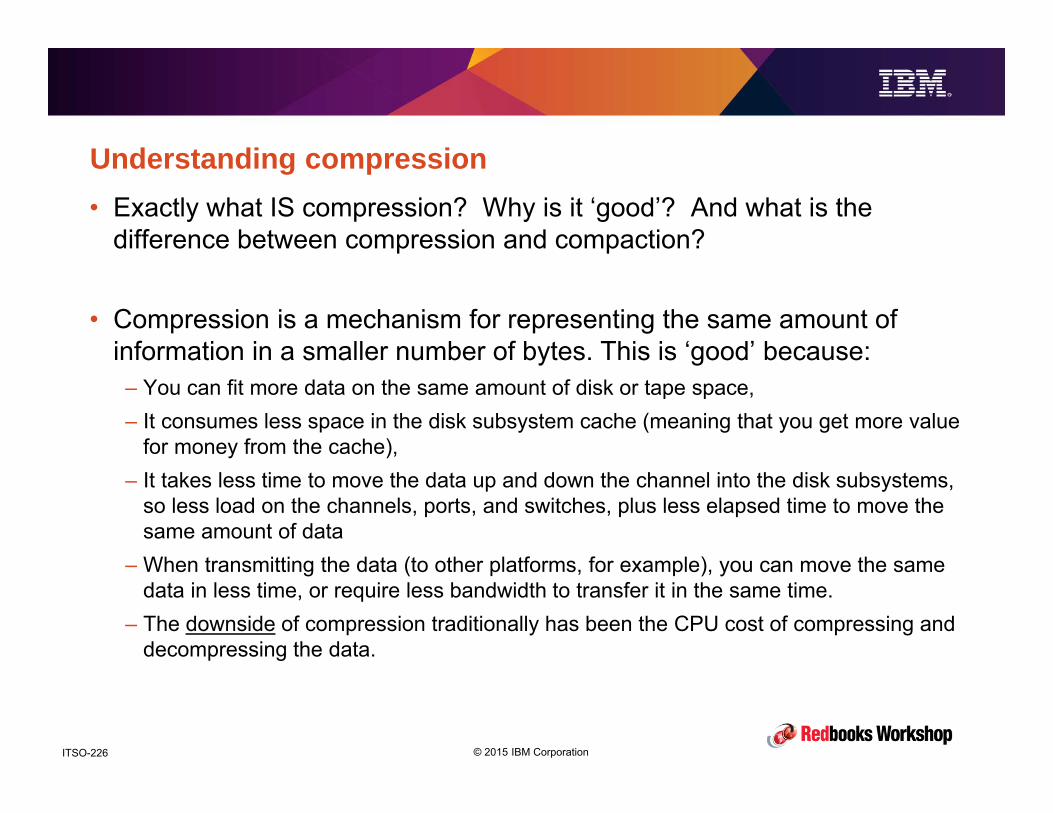
© 2015 IBM CorporationITSO-226
Understanding compression• Exactly what IS compression? Why is it ‘good’? And what is the
difference between compression and compaction?
• Compression is a mechanism for representing the same amount of information in a smaller number of bytes. This is ‘good’ because:
– You can fit more data on the same amount of disk or tape space, – It consumes less space in the disk subsystem cache (meaning that you get more value
for money from the cache), – It takes less time to move the data up and down the channel into the disk subsystems,
so less load on the channels, ports, and switches, plus less elapsed time to move the same amount of data
– When transmitting the data (to other platforms, for example), you can move the same data in less time, or require less bandwidth to transfer it in the same time.
– The downside of compression traditionally has been the CPU cost of compressing and decompressing the data.
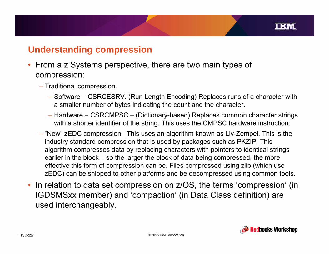
© 2015 IBM CorporationITSO-227
Understanding compression• From a z Systems perspective, there are two main types of
compression:– Traditional compression.
– Software – CSRCESRV. (Run Length Encoding) Replaces runs of a character with a smaller number of bytes indicating the count and the character.
– Hardware – CSRCMPSC – (Dictionary-based) Replaces common character strings with a shorter identifier of the string. This uses the CMPSC hardware instruction.
– “New” zEDC compression. This uses an algorithm known as Liv-Zempel. This is the industry standard compression that is used by packages such as PKZIP. This algorithm compresses data by replacing characters with pointers to identical strings earlier in the block – so the larger the block of data being compressed, the more effective this form of compression can be. Files compressed using zlib (which use zEDC) can be shipped to other platforms and be decompressed using common tools.
• In relation to data set compression on z/OS, the terms ‘compression’ (in IGDSMSxx member) and ‘compaction’ (in Data Class definition) are used interchangeably.

© 2015 IBM CorporationITSO-228
Introduction to zEDC• zEDC is a combination of specialized PCIe cards that
deliver very high performance compression and decompression services, software services to communicate with the card, and exploitation in various software products. It consists of:
– Hardware– Up to 8 PCIe adapters per CPC, max of 2 per PCIe drawer
domain– Up to 15 LPARs sharing each adapter
– IBM recommend a minimum of 4 adapters– And don’t forget your Disaster Recovery CPCs!
– Software– There is a zEDC chargeable feature for z/OS that must be
licensed on every CPC that will use zEDC.
© 2015 IBM CorporationITSO-229
Introduction to zEDC• A very important point that you must understand to avoid confusion about zEDC
is that it is a system service that will compress or decompress data for anyone. For example:
– The data owner might compress the data. As an example, SMF itself calls zEDC to compress the data before it is sent to the log stream. As far as System Logger is concerned, it is being sent 1s and 0s. It is irrelevant to it whether the data was compressed before it was given to it.
– Or, the access method might use zEDC to compress the data. In that case, the user program has no idea that the data is going to be compressed – it just passes the data to BSAM or QSAM. The access method then takes that data, passes it to zEDC, and writes the compressed data to disk.
– Or, you could have something like DFSMSdss, which can (optionally) call zEDC itself, OR it can pass the data to BSAM or QSAM and they can call zEDC, OR, it could call zEDC and pass the compressed data to BSAM or QSAM which might call zEDC again.
• So if someone says that VSAM doesn’t support zEDC, that means that VSAM itself will not call zEDC. However VSAM data sets could happily contain data that had been compressed by zEDC before it was passed to VSAM, as is the case with System Logger offload data sets for compressed SMF log streams.

© 2015 IBM CorporationITSO-230
Potential zEDC benefits• Based on IBM tests and user experiences, IBM expects zEDC to
achieve (on average) about double the compression of traditional z/OS compression techniques. This means SAVINGS ON DASD SPACE, reduced load on disk cache, ports, channels, switches, etc.
– And that is if you already use compression today! If, like many customers, you don’tuse compression because of the CPU cost, zEDC will save you even more DASD SPACE in return for a small increase is CPU time.
• If you compress HSM and/or DSS data that is written to tape today, using zEDC instead of traditional DSS or HSM compression can reduce the number of tapes you are using.
– If you are using a virtual tape subsystem that compresses all incoming data, zEDC will reduce the volume of data being sent through the I/O subsystem and the number of z/OS I/Os.
– Plus, in some cases, compressing the data twice (once with zEDC and once by the tape subsystem) can result in smaller files than if it was only compressed once.

© 2015 IBM CorporationITSO-231
Potential zEDC benefits• Because zEDC moves the load of compressing and decompressing
data from the CPs to the PCIe card, zEDC FREES UP z/OS CPU CAPACITY that was being used to compress data sets.
– One zEDC card costs USD12K. How much does one CP cost?
• Because the capacity used on the zEDC card does not factor into your software bill, it might result in REDUCED SOFTWARE BILLS.
– This depends on whether you were using compression previously, and if the times when a lot of compression/decompression was being done coincided with your peak R4HA.
– Also need to make sure that the capacity freed up by zEDC is not eaten by discretionary work – if it is, your SW bills will not reduce.
• If you encrypt the data, compressing it first reduces the amount of data to be encrypted/decrypted, thereby reducing elapsed time and CPU utilization.
– Additionally, PTF UA72250 enhances the Encryption Facility for z/OS to support zEnterprise Data Compression (zEDC) for OpenPGP messages.

© 2015 IBM CorporationITSO-232
List of zEDC Exploiters• The following IBM products provide exploitation of zEDC at this time:
– SMF (only in logstream mode)– BSAM and QSAM (but not VSAM KSDSs)– DFSMSdss– DFSMShsm when using DFSMSdss as the data mover– IBM Encryption Facility– MQ Series V8– Connect Direct– Zlib services– Java V7– Content Manager OnDemand, starting in 9.5.0.3 (shipped August 14, 2015)
• In all cases, zEDC exploitation is optional, so you must do something to explicitly indicate that you want to use it.

© 2015 IBM CorporationITSO-233
List of zEDC Exploiters
• The following ISV products provide exploitation of zEDC at this time:– Data21– Innovation Data Processing– PKWARE - PKZIP and SecureZip– Alebra - Parallel Data Mover– Software AG - Entire Net-Work– Gzip 1.6 in Rocket Software Ported Tools for z/OS – see
http://www.rocketsoftware.com/free-tools
– If you know of any others, please let us know.

© 2015 IBM CorporationITSO-234
Quantifying zEDC benefits – comparison to traditional compression
• The most common IBM exploiters of zEDC compression at this time are:– Sequential data sets (accessed using BSAM or QSAM)– SMF Log streams– DFSMSdss and hsm
• We ran some comparisons of different types of compression (DFSMS Generic compression, DFSMS Tailored compression (on both zEC12 and z13), and zEDC compression) on 3 different types of data:
– SMF Sequential data sets.– DB2 archive log offloads– SVC dump data sets
• We also ran some comparisons of decompression for the different compression methods.
• And we have some measurements for dss DUMP processing

© 2015 IBM CorporationITSO-235
Performance comparison
• Measurement 1 - SMF.
• 2 data sets containing SMF data, total size 60255 tracks.
• All runs on z13, except Tailored_EC12, which ran on zEC12.
0102030405060
Elapsed time
05
101520
TCB Time
00.05
0.10.15
0.20.25
0.3
SRB Time
0.002.004.006.008.00
Compression ratio
About double
Compression improvements
in z13
Customer experience for SMF compression ratio has been in the 8-10x
range, depending on the SMF record types

© 2015 IBM CorporationITSO-236
Performance comparison
• Measurement 2 – DB2 logs.
• 15 DB2 archive log data sets, total size 32175 tracks.
• All runs on z13, except Tailored_EC12, which ran on zEC12.
24.224.424.624.8
2525.225.425.6
Elapsed time
012345678
TCB Time
00.050.1
0.150.2
0.25
SRB Time
0.00
5.00
10.00
15.00
Compression ratioTypically little
change in SRB time
Consistently around 2x
compression of traditional compression

© 2015 IBM CorporationITSO-237
Performance comparison
• Measurement 3 – SVC dumps.
• 5 SVC dump data sets, total size 40883 tracks.
• All runs on z13, except Tailored_EC12, which ran on zEC12.
3030.5
3131.5
3232.5
3333.5
34
Elapsed time
02468
1012
TCB Time
00.050.1
0.150.2
0.250.3
0.35
SRB Time0.002.004.006.008.00
Compression ratio
z13 reduces traditional
compression CPU time by up to 50% for
both tailored and generic

© 2015 IBM CorporationITSO-238
Performance comparison
• Measurement 4 - decompression.
• Decompression comparisons – uncompressed data set size 60255 tracks.
• Measured on both zEC12 and z13.
• This is for SMF data set on zEC12. Similar pattern for all data types across both
CPCs.
0
10
20
30
40
50
60
NoComp Generic Tailored zEDC
Elapsed time
0
0.5
1
1.5
2
2.5
3
3.5
NoComp Generic Tailored zEDC
TCB Time
0
0.05
0.1
0.15
0.2
0.25
NoComp Generic Tailored zEDC
SRB Time

© 2015 IBM CorporationITSO-239
Performance comparison• Measurement 5 – DFSMSdss DUMP.
• DFSMSdss FULL VOLUME – (on zEC12).
0 100 200 300 400 500 600
No Comp/Std EF
COMPRESS/Std EF
HWCOMPRESS/Std EF
ZCOMPRESS/Std EF
No Comp/zEDC
COMPRESS/zEDC
HWCOMPRESS/zEDC
ZCOMPRESS/zEDC
Elapsed time
DFSMSdsscompression
option
Output data set format
0.000 1.000 2.000 3.000 4.000 5.000
No Comp/Std EF
COMPRESS/Std EF
HWCOMPRESS/Std EF
ZCOMPRESS/Std EF
No Comp/zEDC
COMPRESS/zEDC
HWCOMPRESS/zEDC
ZCOMPRESS/zEDC
Compression Ratio
0.00 100.00 200.00 300.00 400.00
No Comp/Std EF
COMPRESS/Std EF
HWCOMPRESS/Std EF
ZCOMPRESS/Std EF
No Comp/zEDC
COMPRESS/zEDC
HWCOMPRESS/zEDC
ZCOMPRESS/zEDC
CPU time

© 2015 IBM CorporationITSO-240
Identifying potential benefit of zEDC• At this time, the only tool available from IBM to help you estimate the
potenial cost and savings of zEDC only handles sizing for BSAM/QSAM use of zEDC – IBM’s zSystems Batch Network Analyzer (zBNA).
• zBNA can be downloaded at no charge(!) from http://www-03.ibm.com/support/techdocs/atsmastr.nsf/WebIndex/PRS5132
• While there are other easy-to-implement exploiters of zEDC, there are currently no tools to help you identify the value that zEDC will deliver for them.
– However it is likely that zEDC can be cost justified for use with sequential data sets alone. Savings through additional exploitation of zEDC are a bonus.

© 2015 IBM CorporationITSO-241
Identifying potential benefit of zEDC
• zBNA uses data from SMF Type 14, 15, 30, 42(6), 70, 72, and 113 records.
– Run CP3KEXTR against these SMF records to create input file for zBNA. Input should only
contain records from one system for one night – loading larger volumes of data can result in
‘878’ abends in zBNA.
– To save time, TERSE the resulting file on z/OS and download that file to your PC. zBNA can input
the tersed file directly.
• zBNA has been receiving a stream of enhancements to its zEDC support, so
make sure that you download the latest version and review the What’s New
section on the web site to see the list of recent new functions.
• If you are not familiar with zBNA, download the handouts from http://share.org
for John Burg’s zBNA hands-on lab – Session 17551 System z Batch Network
Analyzer (zBNA) Tool Hands-on Lab and get sample data from the IBM
Techdocs web site, in the Education section.
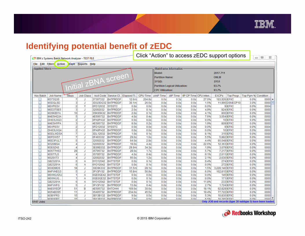
© 2015 IBM CorporationITSO-242
Identifying potential benefit of zEDCClick “Action” to access zEDC support options

© 2015 IBM CorporationITSO-243
Identifying potential benefit of zEDC
Actual compression ratio for compressed
data sets
List of 50 largest SEQ data sets.Click Action to
change number of data sets displayed.
Can sort on any column
ESTIMATES of the impact of
enabling zEDC
Default is to include ALL data sets
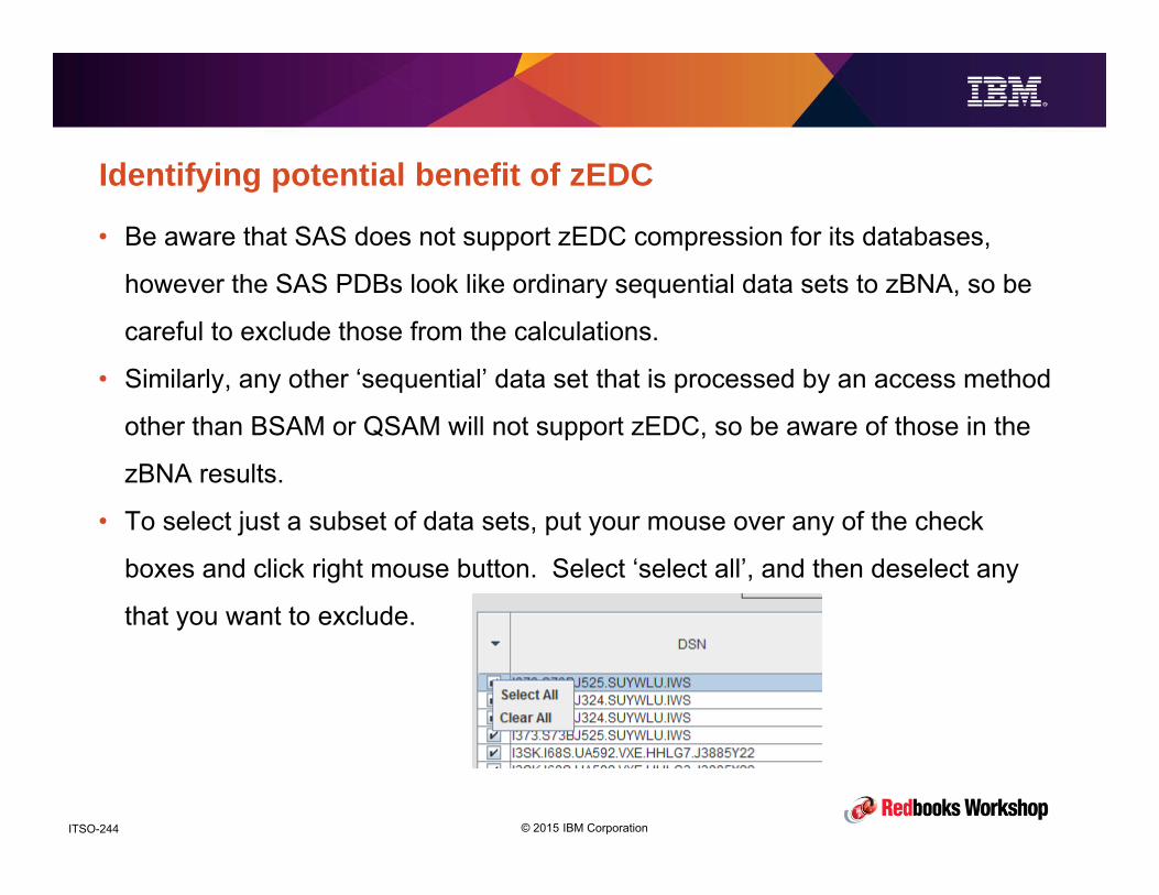
© 2015 IBM CorporationITSO-244
Identifying potential benefit of zEDC
• Be aware that SAS does not support zEDC compression for its databases,
however the SAS PDBs look like ordinary sequential data sets to zBNA, so be
careful to exclude those from the calculations.
• Similarly, any other ‘sequential’ data set that is processed by an access method
other than BSAM or QSAM will not support zEDC, so be aware of those in the
zBNA results.
• To select just a subset of data sets, put your mouse over any of the check
boxes and click right mouse button. Select ‘select all’, and then deselect any
that you want to exclude.

© 2015 IBM CorporationITSO-245
Identifying potential benefit of zEDC
Estimated number of zEDC cards required for
THIS system
Apply PTF for OA42195 to get
accurate numbers here
This chart only provides capacity info
– does not allow for resiliency
About 60% of one card.

© 2015 IBM CorporationITSO-246
Identifying potential benefit of zEDC
This is the additional CPU cost of calling
zEDC.
About 80% of one CP.CPU seconds saved per
hour on this system This report is based on a system
running on a z196.

© 2015 IBM CorporationITSO-247
Identifying potential benefit of zEDC
Don’t forget that lower I/O rates result in lower RNIs, meaning more MIPS.
Estimated reduction in number of I/Os per hour

© 2015 IBM CorporationITSO-248
Identifying potential benefit of zEDC
By default, all these charts assume that you will enable zEDC for ALL sequential data sets. To change, select a different option in Graphing Options
Estimated reduction in number of GBs per hour

© 2015 IBM CorporationITSO-249
Identifying potential benefit of zEDC
• Few tips for using zBNA:
– zEDC provides 3 potential savings:
– DASD and tape space savings – should apply to EVERYONE
– Free up CP capacity – should apply to EVERYONE
– Reduced software bills.
– To achieve this benefit, you must be using compression today, and your peak Rolling 4-
Hour Average must coincide with your peak compression activity.
– But don’t get hung on just this savings – the other two savings are real as well.
– Remember that zBNA is only looking at one exploiter of zEDC. It does not do anything for SMF or
zlib or MQ or Connect Direct or .... So if you plan to use additional exploiters, the benefit of zEDC is
likely to be larger.

© 2015 IBM CorporationITSO-250
Configuring zEDC using HCD• The ITSO have created 2 excellent videos that lead you step-by-step through the
process of defining a zEDC card in HCD. For info on how to add a zEDC card (in
less than 7 minutes!), refer to:
– https://www.youtube.com/watch?v=5We571gvh5o and
– https://www.youtube.com/watch?v=wZbtM77ubrs– Recommend using PFIDs starting with an even digit for one Resource Group, and an odd digit for the other
Resource Group. Then make sure that every LPAR is connected to at least one card in each Resource
Group (recommended minimum of 2 cards).
• After the hardware setup is complete, you need to update the IFAPRDxx
member to enable zEDC (this requires an IPL).
• IF you have unauthorized programs using the zlib interface to zEDC,
they must have READ access to the zEDC SAF profile
(FPZ.ACCELERATOR.COMPRESSION.)
© 2015 IBM CorporationITSO-251
How to enable zEDC exploitation – SMF Log streams• The first exploiter of zEDC was SMF (when in log stream mode). This is a very
popular starting point because the implementation effort is trivial and the savings can be significant.
– SMF is also nice because the heaviest volume of SMF records is typically during the online day when other use of zEDC (sequential data sets, HSM, DSS) is typically light.
• To exploit zEDC, SMF must be writing its records to log streams. SYS1.MAN data sets are not and will not be supported for zEDC compression. If you are already in log stream mode, you are 99% of the way there.
• To enable compression of an SMF log stream, add the COMPRESS keyword to the LSNAME or DEFAULTLSNAME definition in SMFPRMxx:
– DEFAULTLSNAME(IFASMF.DEFAULT,COMPRESS) DSPSIZMAX(200M)
– You can have a mix of some log streams that are using zEDC and ones that are not.

© 2015 IBM CorporationITSO-252
How to enable zEDC exploitation – SMF Log streams
• Each log block has an indication of whether it contains zEDC-compressed data or not. When IFASMFDL reads the log block, it knows whether it needs to be decompressed or not. This allows you to have a mix of compressed and not-compressed log blocks in the same log stream (allows for a phased implementation of zEDC compression of shared SMF log streams across multiple systems).
SMFEWTM IXGWrite
SMF 64k Buffers
Application Generating
SMF Records
Long-term Storage
End User Applications
CFMedia Manager
Offload Data sets
IFASMFDL
deflate
inflate
Up to 16 64K requests per log stream
© 2015 IBM CorporationITSO-253
How to enable zEDC exploitation – SMF Log streams
• Summary
– That’s it – just one new keyword in your SMFPRMxx member, no additional changes
required.
– Compression of a log stream can be turned on and off dynamically.
– But be aware that if you want to turn it OFF, removing the COMPRESS keyword will
not achieve that – you must change COMPRESS to NOCOMPRESS.
– IFASMFDL is the only way to read the SMF log stream, and it automatically detects
whether a log block is compressed or not, meaning that no JCL or Parm changes are
required.
– To get the best value from zEDC, your SMF offload sequential data sets should use a
data class that specifies the use of zEDC compression.
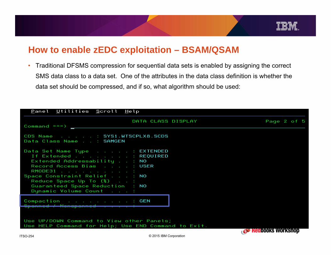
© 2015 IBM CorporationITSO-254
How to enable zEDC exploitation – BSAM/QSAM• Traditional DFSMS compression for sequential data sets is enabled by assigning the correct
SMS data class to a data set. One of the attributes in the data class definition is whether the
data set should be compressed, and if so, what algorithm should be used:

© 2015 IBM CorporationITSO-255
How to enable zEDC exploitation – BSAM/QSAM
• To enable zEDC compression, we recommend setting up a new data class for
testing purposes. That data class should be defined with zEDC REQUIRED:

© 2015 IBM CorporationITSO-256
How to enable zEDC exploitation – BSAM/QSAM
• You then conduct your testing by specifying the correct data class when you
allocate the data set.
• Testing should include allocation, deletion, extending the data set, filling the
data set, partial release, single strip, multiple stripe, varying buffer numbers,
backup, migration, recall, restore…..
• When testing is complete, update the previous compression data classes to
indicate ZR (zEDC required), and (optionally) update the COMPRESS
parameter in IGDSMSxx.

© 2015 IBM CorporationITSO-257
How to enable zEDC exploitation – DFSMSdss & hsm
• Obvious candidates for zEDC exploitation are DFSMSdss and DFSMShsm
– The data sets they create are not actively used, so the ratio of decompressions to compressions
should be low.
– You want to balance data availability and protection with minimal disk or tape space usage.
– Both already provide compression options that use software compression, so are good potentials
for CPU savings if you can replace their traditional compression with zEDC.
• Ability to use zEDC to compress and decompress data was added in z/OS 2.1 +
APARs (OA42198, OA42238, and OA42243).
– z/OS 1.12 and 1.13 can read zEDC-compressed data sets, but use software (extremely CPU-
intensive) to do it.
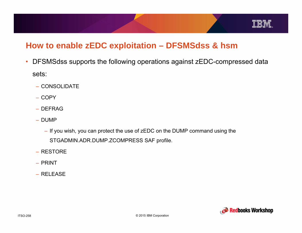
© 2015 IBM CorporationITSO-258
How to enable zEDC exploitation – DFSMSdss & hsm
• DFSMSdss supports the following operations against zEDC-compressed data
sets:
– CONSOLIDATE
– COPY
– DEFRAG
– DUMP
– If you wish, you can protect the use of zEDC on the DUMP command using the
STGADMIN.ADR.DUMP.ZCOMPRESS SAF profile.
– RESTORE
– RELEASE

© 2015 IBM CorporationITSO-259
How to enable zEDC exploitation – DFSMSdss & hsm
• Most of the DFSMSdss support for zEDC is related to processing data sets that have
already been compressed by zEDC.
– It doesn’t make sense to decompress the data, then immediately compress it again.
– DFSMSdss understands which data sets are in zEDC-compressed format and reads the data as-is (without
calling zEDC) from the source volume where appropriate (COPY, for example).
– For most dss operations, the data is then written as-is to the output data set.
• For DUMP operations against zEDC-compressed data sets, there are two options:
– If you specify ZCOMPRESS in the dss SYSIN, dss passes the data to zEDC to be further compressed and
it is then written to DASD. In this case, the output data set can be EF or non-EF.
– If the output data set is in extended format (based on the data class), dss writes very large blocks (of
already zEDC-compressed data) to BSAM. If the data class indicates that zEDC should be used, BSAM
then calls zEDC to compress the data again before writing it to the output data set.
• Note that dss COPY does NOT support the ZCOMPRESS keyword.
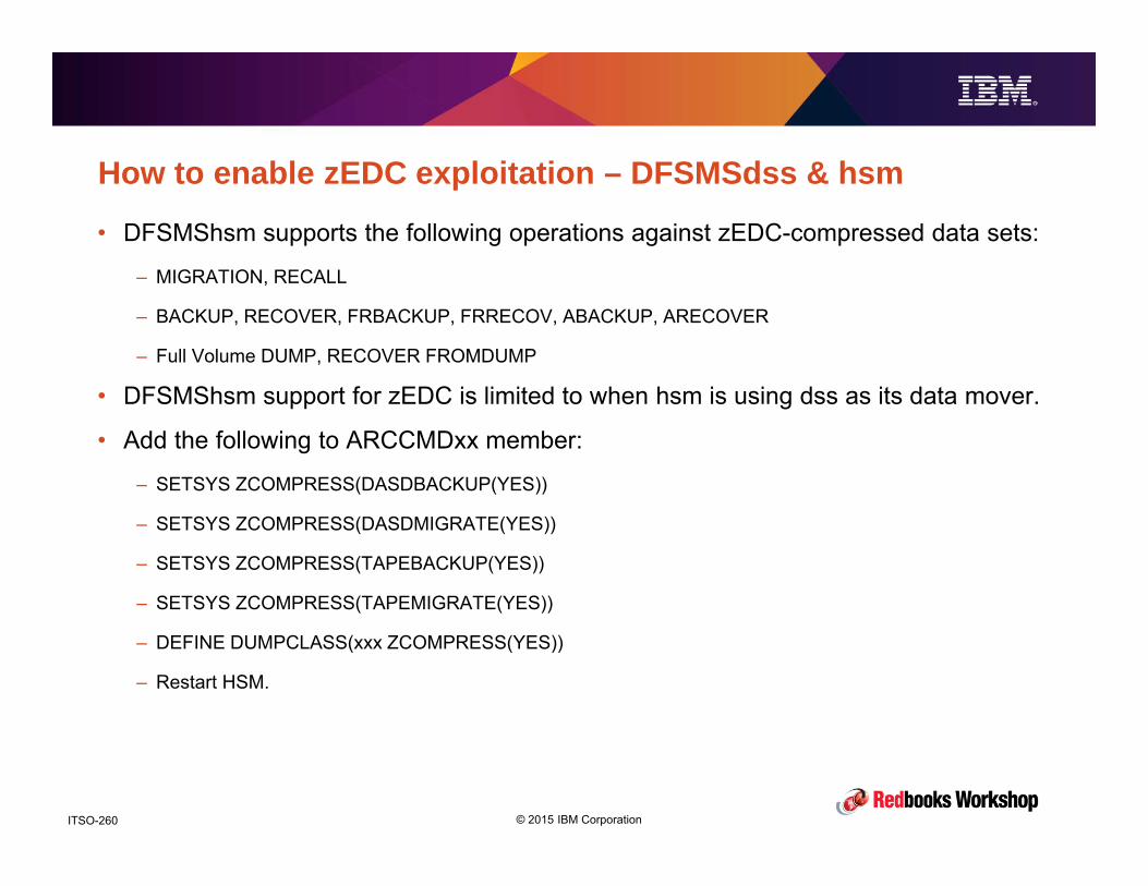
© 2015 IBM CorporationITSO-260
How to enable zEDC exploitation – DFSMSdss & hsm
• DFSMShsm supports the following operations against zEDC-compressed data sets:
– MIGRATION, RECALL
– BACKUP, RECOVER, FRBACKUP, FRRECOV, ABACKUP, ARECOVER
– Full Volume DUMP, RECOVER FROMDUMP
• DFSMShsm support for zEDC is limited to when hsm is using dss as its data mover.
• Add the following to ARCCMDxx member:
– SETSYS ZCOMPRESS(DASDBACKUP(YES))
– SETSYS ZCOMPRESS(DASDMIGRATE(YES))
– SETSYS ZCOMPRESS(TAPEBACKUP(YES))
– SETSYS ZCOMPRESS(TAPEMIGRATE(YES))
– DEFINE DUMPCLASS(xxx ZCOMPRESS(YES))
– Restart HSM.

© 2015 IBM CorporationITSO-261
How to enable zEDC exploitation – DFSMSdss & hsm
• DFSMShsm can use zEDC to compress any data set type except for PDS when
migrating or backing up the data.
• But, DFSMShsm will NOT call zEDC to compress an already-compressed data
set.
– Like dss, HSM will copy already-compressed data sets to its output data sets without
decompressing and then recompressing them.
– Same applies on a RECALL of a data set that was previously compressed on Primary DASD.

© 2015 IBM CorporationITSO-262
How to enable zEDC exploitation – DFSMSdss & hsm
• DFSMSdss/zEDC tips…
– Compression ratio is very dependent on input data. In DFSMS lab measurements, compression
ratios ranged between 3:1 and 9:1.
– In ITSO measurements, HWCOMPRESS consistently used the most CPU. This was on a zEC12,
would expect it to be better on z13. But users of HWCOMPRESS are still expected to see the
largest savings from moving to zEDC.
– Compare the ZCOMPRESS/EF run to the NoComp/zEDC run – both call zEDC once, but dss
passes more data at a time to BSAM when using zEDC-format output data sets, possibly resulting
in better compression ratios.
– If using DFSMSdss DUMP to write to tape, you should specify ZCOMPRESS rather than
COMPRESS or HWCOMPRESS – data class with COMPACT(ZR or ZP) will not work for tape data
set..
– Even if input data set has already been compressed with zEDC, it may be possible to get further
compression improvements on DUMP (to tape) with ZCOMPRESS or DUMP to zEDC-compressed
(disk) data set.
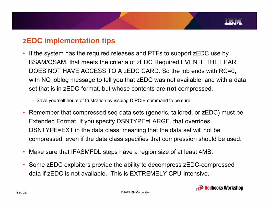
© 2015 IBM CorporationITSO-263
zEDC implementation tips• If the system has the required releases and PTFs to support zEDC use by
BSAM/QSAM, that meets the criteria of zEDC Required EVEN IF THE LPAR DOES NOT HAVE ACCESS TO A zEDC CARD. So the job ends with RC=0, with NO joblog message to tell you that zEDC was not available, and with a data set that is in zEDC-format, but whose contents are not compressed.
– Save yourself hours of frustration by issuing D PCIE command to be sure.
• Remember that compressed seq data sets (generic, tailored, or zEDC) must be Extended Format. If you specify DSNTYPE=LARGE, that overrides DSNTYPE=EXT in the data class, meaning that the data set will not be compressed, even if the data class specifies that compression should be used.
• Make sure that IFASMFDL steps have a region size of at least 4MB.
• Some zEDC exploiters provide the ability to decompress zEDC-compressed data if zEDC is not available. This is EXTREMELY CPU-intensive.
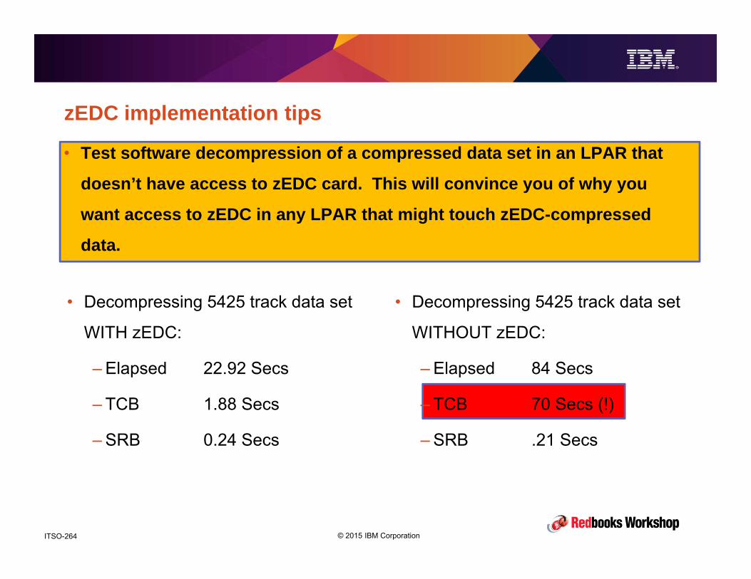
© 2015 IBM CorporationITSO-264
zEDC implementation tips
• Test software decompression of a compressed data set in an LPAR that
doesn’t have access to zEDC card. This will convince you of why you
want access to zEDC in any LPAR that might touch zEDC-compressed
data.
• Decompressing 5425 track data set
WITH zEDC:
– Elapsed 22.92 Secs
– TCB 1.88 Secs
– SRB 0.24 Secs
• Decompressing 5425 track data set
WITHOUT zEDC:
– Elapsed 84 Secs
– TCB 70 Secs (!)
– SRB .21 Secs
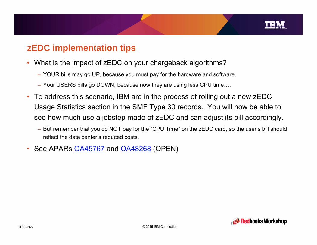
© 2015 IBM CorporationITSO-265
zEDC implementation tips• What is the impact of zEDC on your chargeback algorithms?
– YOUR bills may go UP, because you must pay for the hardware and software.
– Your USERS bills go DOWN, because now they are using less CPU time….
• To address this scenario, IBM are in the process of rolling out a new zEDCUsage Statistics section in the SMF Type 30 records. You will now be able to see how much use a jobstep made of zEDC and can adjust its bill accordingly.
– But remember that you do NOT pay for the “CPU Time” on the zEDC card, so the user’s bill should reflect the data center’s reduced costs.
• See APARs OA45767 and OA48268 (OPEN)

© 2015 IBM CorporationITSO-266
zEDC implementation tips
• An important zEDC PTF is UA77619 (ABEND11E-0702 OR ABEND002-F6 in
job using zEDC). The PTF is available, but one of the pre-reqs is PE.
• However you can force on the pre-req PTF if you specify
FREEMAINEDFRAMES(NO) in DIAGxx. For more information, see APAR
OA46291.

© 2015 IBM CorporationITSO-267
zEDC implementation tips
• If you are using CICS SMF record compression and/or DB2 record compression
today, those functions use software compression, not zEDC.
• Recommend that you turn off CICS and DB2 SMF record compression after
you implement zEDC compression for the associated SMF log streams.
– zEDC will provide at least as good compression, probably more.
– AND you save the CPU cost in CICS and DB2.

© 2015 IBM CorporationITSO-268
zEDC implementation tips• If you want to take zEDC on and offline for testing purposes (or to see how
exploiters react if zEDC goes away):– Issue D PCIE to get PFID for zEDC devices
D PCIE IQP022I 13.58.49 DISPLAY PCIE 376 PCIE 0012 ACTIVE PFID DEVICE TYPE NAME STATUS ASID JOBNAME PCHID VFN 00000025 Hardware Accelerator ALLC 0013 FPGHWAM 01BC 000600000035 Hardware Accelerator ALLC 0013 FPGHWAM 027C 0006
– Issue CF PFID(xx),OFFLINE,FORCE for each device:CF PFID(25),OFFLINE,FORCE IQP034I PCIE FUNCTION 00000025 NOT AVAILABLE FOR USE. 405 PCIE DEVICE TYPE NAME = (Hardware Accelerator ).
IQP034I PCIE FUNCTION 00000025 AVAILABLE FOR CONFIGURATION.PCIE DEVICE TYPE NAME = (Hardware Accelerator ).
IEE505I PFID(25),OFFLINE IEE712I CONFIG PROCESSING COMPLETE
• To bring devices back online, issue CF PFID(xx),ONLINE• If you config off all zEDC cards while SMF is using compression, you will get
nasty message IFA730E, but SMF continues writing to the log stream, but without compressing the records.

© 2015 IBM CorporationITSO-269
zEDC implementation tips• When maintenance is applied to zEDC cards (a hardware function), all the cards
in one of the two Resource Groups will be taken offline.
• To ensure that zEDC remains available, every LPAR should be connected to at least 1 zEDC card in each Resource Group.
– This means that you should ALWAYS have a minimum of two zEDC cards on a CPC. If you only have one, you may need to pause processing for any workload using zEDC while maintenance is being applied.
• To cater for the possibility of one of the surviving cards failing while maintenance is being applied to the other Resource Group, IBM recommend that each LPAR should be connected to 4 zEDC cards.
• Apply the PTF for APAR OA48434 – this is a Health Check to ensure that the LPAR has access to more than one zEDC card. Enable the check and add the check message to your automation to ensure that the appropriate personnel are notified if a card becomes unavailable.

© 2015 IBM CorporationITSO-270
Monitoring zEDC performance
• The bandwidth of the zEDC card is over 1GB/sec.
– Compare this to about 300 MB/sec for the CMPSC instruction and between 50 and 100MB/sec for
zlib.
• In our test with 16 parallel compression jobs running, we couldn’t drive the
utilization of the card above 34%. So, for most customers, 2 cards should
provide sufficient capacity.
• If you find that utilization of the card is increasing, that is a GOOD THING,
because it means that work that would previously have run on a general
purpose CP (and that would have been counted in the determination of your
software bills) is now being processed on a cheaper, faster processor AND is
not impacting your software bills.
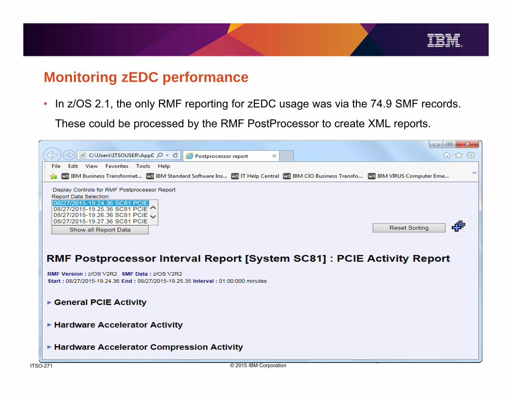
© 2015 IBM CorporationITSO-271
Monitoring zEDC performance
• In z/OS 2.1, the only RMF reporting for zEDC usage was via the 74.9 SMF records.
These could be processed by the RMF PostProcessor to create XML reports.
© 2015 IBM CorporationITSO-272
Monitoring zEDC performance
• In the following reports, system SC81 (z/OS 2.2) was running 16 concurrent
IEBGENERs, copying uncompressed data sets to zEDC-compressed data sets.
The only zEDC activity in system SC80 (z/OS 2.1) was a small amount of SMF
activity, writing to zEDC-compressed log streams.

© 2015 IBM CorporationITSO-273
Monitoring zEDC performance
Note that the same report template is used for RoCE and zEDC, so some fields will be empty in the reports for zEDC devices.
A
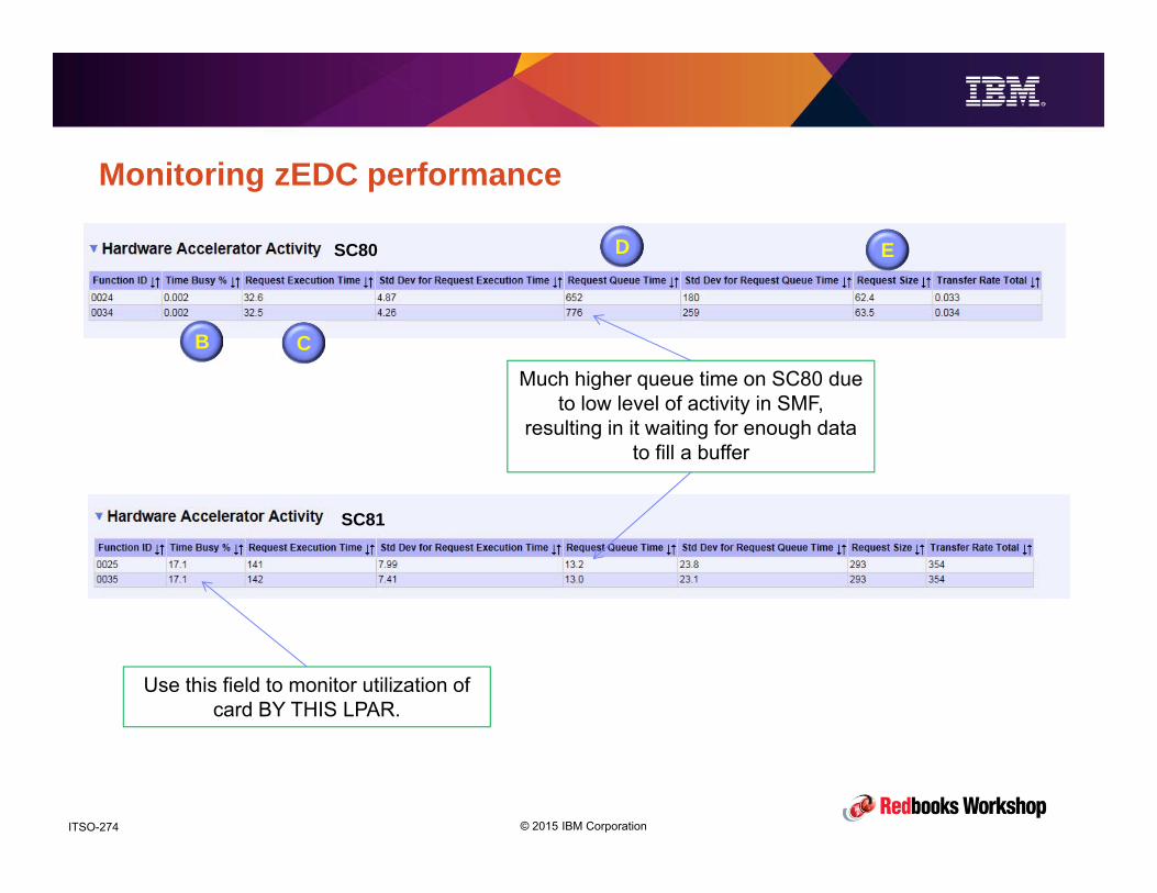
© 2015 IBM CorporationITSO-274
Monitoring zEDC performance
SC80
SC81
Much higher queue time on SC80 due to low level of activity in SMF,
resulting in it waiting for enough data to fill a buffer
Use this field to monitor utilization of card BY THIS LPAR.
CB
D E

© 2015 IBM CorporationITSO-275
Monitoring zEDC performance
SC80
SC81
Remember that this report includes total numbers for ALL exploiters. To get
information for a specific exploiter, need to go to info provided by that exploiter
KJ
HGF
I
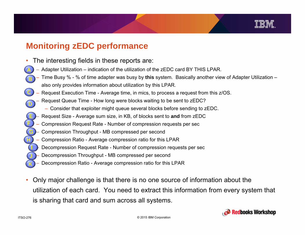
© 2015 IBM CorporationITSO-276
Monitoring zEDC performance• The interesting fields in these reports are:
– Adapter Utilization – indication of the utilization of the zEDC card BY THIS LPAR.– Time Busy % - % of time adapter was busy by this system. Basically another view of Adapter Utilization –
also only provides information about utilization by this LPAR.– Request Execution Time - Average time, in mics, to process a request from this z/OS.– Request Queue Time - How long were blocks waiting to be sent to zEDC?
– Consider that exploiter might queue several blocks before sending to zEDC.– Request Size - Average sum size, in KB, of blocks sent to and from zEDC– Compression Request Rate - Number of compression requests per sec– Compression Throughput - MB compressed per second– Compression Ratio - Average compression ratio for this LPAR– Decompression Request Rate - Number of compression requests per sec– Decompression Throughput - MB compressed per second– Decompression Ratio - Average compression ratio for this LPAR
• Only major challenge is that there is no one source of information about the utilization of each card. You need to extract this information from every system that is sharing that card and sum across all systems.
C
D
E
BA
F
HI
JK
G

© 2015 IBM CorporationITSO-277
Monitoring zEDC performance
• RMF in z/OS 2.2 added the ability to display a subset of zEDC information using
Monitor III (Option 3.14 PCIE)
Move cursor to PFID and press enter to get more useful information

© 2015 IBM CorporationITSO-278
Monitoring zEDC performance
• This display provides much more useful info. Note that all the info only relates
to this LPAR’s use of the card.

© 2015 IBM CorporationITSO-279
Other monitoring information for zEDC• All the information in the Monitor III display (both primary panel and the
cursor-sensitive field display) is also available using the RMF Overview reports function – see section “PCIE Function Activity - SMF record type 74-9” in the RMF User’s Guide.
• The collection of PCIE data by RMF is controlled by the PCIE keyword in ERBRMF04 member – it is ENabled by default.

© 2015 IBM CorporationITSO-280
Other monitoring information for zEDC• How do you know when you need more zEDC capacity?
– The zEDC card works on a simple round robin polling mechanism, checking each LPAR it is connected to, to see if they have any work for it.
– If no work, it tries the next LPAR.
– As the card utilization increases, the interval between when it polls each LPAR gets larger, potentially resulting in queueing for longer in the z/OS images.
– The queue time is reported in the RMF PCIE report (“Request Queue Time”).
– Unlike zIIPs, there is no overflow to general purpose CPs – if the card is overloaded, users of its services will simply observe longer queue times.
– So, the point at which you need more zEDC capacity is determined by how much queue time you are willing to tolerate.
– Queue time is determined by normal queue time formula. With more ‘servers’ (more zEDC cards), you can run at higher utilizations before queue time increases.

© 2015 IBM CorporationITSO-281
Other monitoring information for zEDC• As part of APAR OA42195, the SMF Type 14/15 records have new flags and
fields related to zEDC:– Offsets Name Length Format Description
– 6 (6) SMF14CDL 8 binary Number of bytes of compressed data read or written since this open.
– 14 (E) SMF14UDL 8 binary Number of bytes of data read or written since this open (data length prior to compression).
– 22 (16) SMF14CDS 8 binary Size of the compressed format data set (number of compressed user data bytes).
– 30 (1E) SMF14UDS 8 binary Size of the compressed format data set (number of uncompressed user data bytes).
– 80 (50) SMF14CMPTYPE 1 binary Compression Type
– Meaning When Set
– 0 SMF14CMPTYPENA Not compressed format or Unknown
– 1 SMF14CMPTYPEGEN Generic Compression
– 2 SMF14CMPTYPETLRD Tailored Compression
– 3 SMF14CMPTYPEZEDC zEDC Compression
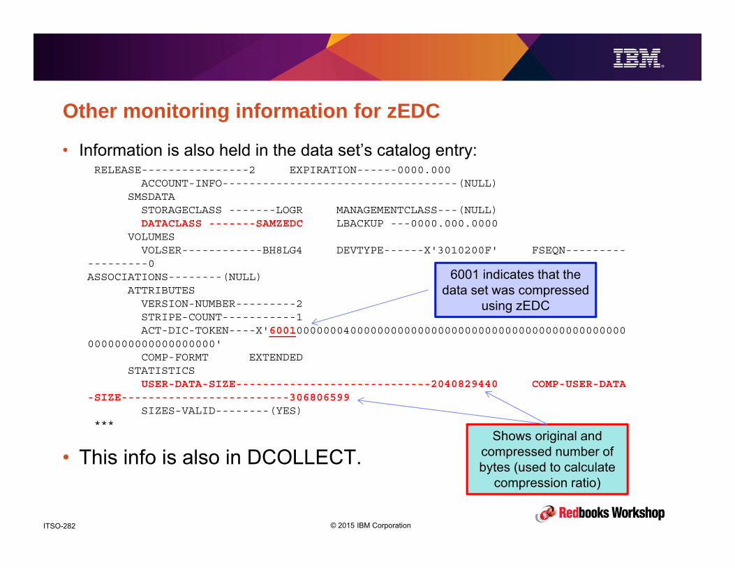
© 2015 IBM CorporationITSO-282
Other monitoring information for zEDC
• Information is also held in the data set’s catalog entry:RELEASE----------------2 EXPIRATION------0000.000
ACCOUNT-INFO-----------------------------------(NULL) SMSDATA
STORAGECLASS -------LOGR MANAGEMENTCLASS---(NULL) DATACLASS -------SAMZEDC LBACKUP ---0000.000.0000
VOLUMES VOLSER------------BH8LG4 DEVTYPE------X'3010200F' FSEQN---------
---------0 ASSOCIATIONS--------(NULL)
ATTRIBUTES VERSION-NUMBER---------2 STRIPE-COUNT-----------1 ACT-DIC-TOKEN----X'60010000000400000000000000000000000000000000000000000
0000000000000000000' COMP-FORMT EXTENDED
STATISTICS USER-DATA-SIZE-----------------------------2040829440 COMP-USER-DATA
-SIZE-------------------------306806599SIZES-VALID--------(YES)
***
• This info is also in DCOLLECT.
6001 indicates that the data set was compressed
using zEDC
Shows original and compressed number of bytes (used to calculate
compression ratio)
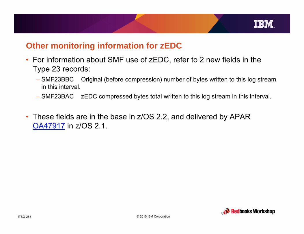
© 2015 IBM CorporationITSO-283
Other monitoring information for zEDC• For information about SMF use of zEDC, refer to 2 new fields in the
Type 23 records:– SMF23BBC Original (before compression) number of bytes written to this log stream
in this interval. – SMF23BAC zEDC compressed bytes total written to this log stream in this interval.
• These fields are in the base in z/OS 2.2, and delivered by APAR OA47917 in z/OS 2.1.
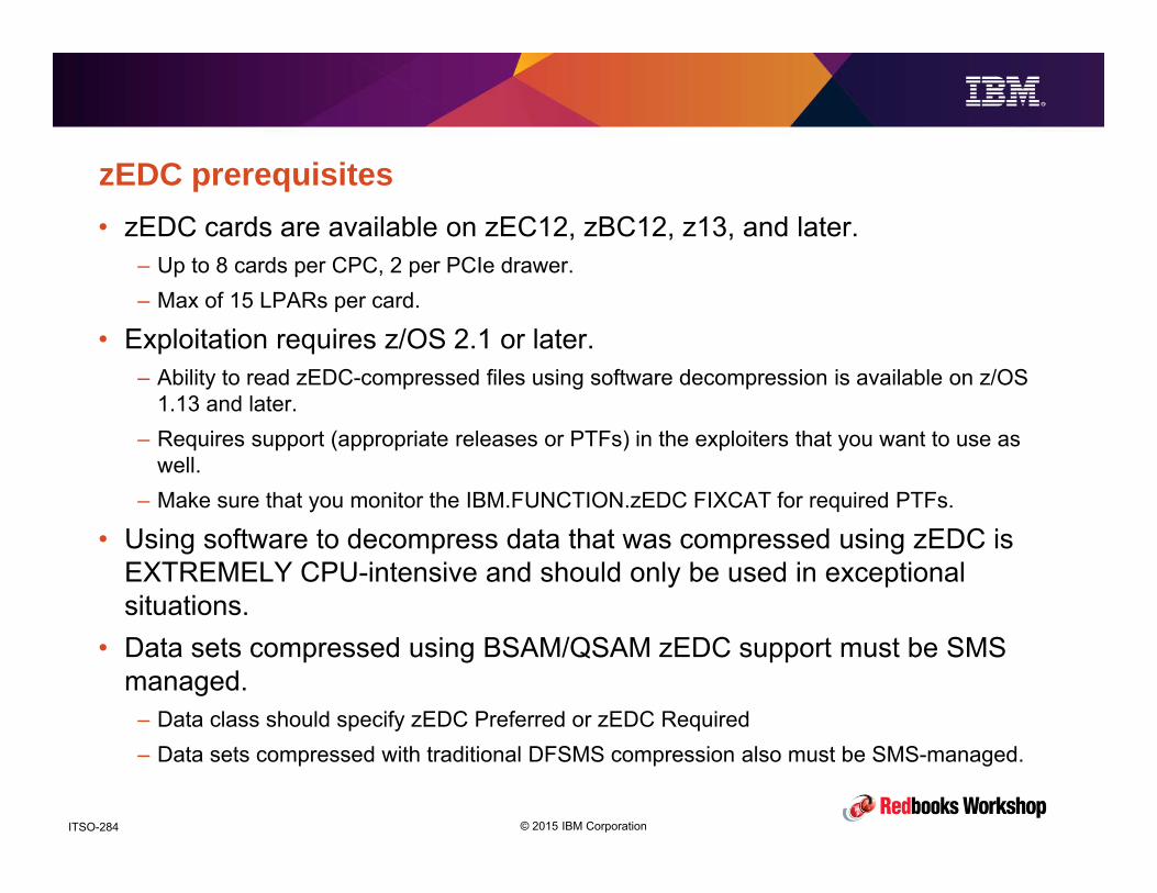
© 2015 IBM CorporationITSO-284
zEDC prerequisites• zEDC cards are available on zEC12, zBC12, z13, and later.
– Up to 8 cards per CPC, 2 per PCIe drawer.– Max of 15 LPARs per card.
• Exploitation requires z/OS 2.1 or later.– Ability to read zEDC-compressed files using software decompression is available on z/OS
1.13 and later.– Requires support (appropriate releases or PTFs) in the exploiters that you want to use as
well.– Make sure that you monitor the IBM.FUNCTION.zEDC FIXCAT for required PTFs.
• Using software to decompress data that was compressed using zEDC is EXTREMELY CPU-intensive and should only be used in exceptional situations.
• Data sets compressed using BSAM/QSAM zEDC support must be SMS managed.
– Data class should specify zEDC Preferred or zEDC Required– Data sets compressed with traditional DFSMS compression also must be SMS-managed.

© 2015 IBM CorporationITSO-285
Summary• Initial take-up of zEDC was slow because you must have zEC12 or later and
z/OS 2.1 or later AND you want those on every system that will share the data, and it is only now that those configurations are becoming common.
• Customer experiences so far have been very positive. One customer described zEDC as ‘a game changer’.
• Download and run zBNA – it has many uses in addition to planning for zEDC, so everyone should have it anyway.
• Once the hardware and software are in place, the implementation of zEDC is simple.
• Recommend to start with SMF, then move on to DFSMSdss and hsm, and then all large sequential data sets.
• Tell anyone that is responsible for large file transfers to and from z/OS about the benefits they might be able to get from zEDC.

© 2015 IBM CorporationITSO-286
zEDC Reference Information• IBM Redbook SG24-8259, Reduce Storage Occupancy and Increase Operations Efficiency with
IBM zEnterprise Data Compression
• IBM RedPaper, REDP-5158, zEDC Compression: DFSMShsm Sample Implementation
• z/OSMF Workflow IBM: z/OS V2R1 zEnterprise® Data Compression Setup Workflow
• zEDC Product Manual SA23-1377, z/OS MVS Programming: Callable Services for High-Level
Languages
• IBM Manual SA23-1380, z/OS MVS Initialization and Tuning Reference
• IBM Hot Topics August 2014, Save BIG with QSAM/BSAM compression by using zEDC and All
aboard with zEDC.
• IBM Hot Topics August 2013, z Enterprise Data Compression Express
• IBM Journal of R&D, Volume 59, Number 4/5, July/Sep. 2015, Integrated high-performance data
compression in the IBM z13
• For a list of zEDC articles created by its lead designer, refer to
https://www.linkedin.com/pub/anthony-sofia/4/6aa/713
• Multiple excellent SHARE presentations by Anthony Sofia, Barbara McDonald, Cecilia Lewis,
and Glenn Wilcock.

© 2015 IBM CorporationITSO-287
Planned Outage ConsiderationsPerformance and Availability

© 2015 IBM CorporationITSO-288
What is in this section?
• Definition of ‘Planned Outage’
• Spare LPAR/system concept.
• Use of system symbols as an availability tool

© 2015 IBM CorporationITSO-289
Definition of planned outage
• 40 years ago, a planned outage meant that you had told the 20 CICS users in
your company that ‘the computer’ would be down this weekend.
• What does ‘planned’ mean today? Is it planned if thousands of customers that
might access your systems have not been told that the system will be down this
weekend?
– And even if you could tell them in advance, do people consider any outage to be acceptable any
more?
• Is there still a requirement for planned outages? And are they acceptable to
your business? How has technology changed in the 40 years?

© 2015 IBM CorporationITSO-290
Planned outages• Are scheduled outages still necessary?
– IBM has had a constant flow of enhancements (and two supporting Redbooks) to let you change things
dynamically that previously would have required a system or subsystem restart.
– These are not intended to eliminate outages – they are intended to give you more control over when you
have a scheduled outage.
– For more information, see the following Redbooks:
– z/OS Planned Outage Avoidance Checklist, SG24-7328
– Improving z/OS Application Availability by Managing Planned Outages, SG24-8178
• However, there are still situations where you need to perform an IPL:– Applying preventive or corrective service, especially in large numbers.
– Applying integrity APARs (Is everyone familiar with the System z Security Portal?)
– Operating system upgrade.
– CPC upgrade.
– Change a system setting that does not support dynamic changes.
– Does anyone still IPL for the Daylight Savings Time change? This is one that should NOT be necessary.

© 2015 IBM CorporationITSO-291
Definition of planned outage
• Given that we are unlikely to eliminate the need for scheduled outages for the
foreseeable future, how do we balance technical requirements with business ones?
• For applications that DO support data sharing and dynamic transaction routing, a
system outage (especially a planned one) should be transparent or nearly
transparent, so application availability needs should not stop a scheduled outage.
• For your other applications:
– If they are important enough to stop a system from being IPLed, then they should support data sharing. It
is not good business to have a non-critical system stopping the application of service that makes the critical
applications more resilient/secure.
– At the same time, we want to make the outage as painless as possible for everyone.
© 2015 IBM CorporationITSO-292
Minimizing outage time
• For the non-data sharing applications, the down time typically ranges from about
30 minutes, to the entire length of the system outage.
• The typical options are:
– Shut the application down and leave it down for the duration of the outage.
– Stop the application, move it to another system (one outage), make your changes to the system and
bring it back up, stop the application again, and move it back to the original system.
• The first methodology results in a longer application outage.
• The second often results in more problems as a result of moving all the
applications around, particularly those with affinities between them.
© 2015 IBM CorporationITSO-293
Minimizing outage time – The Dunkan Doctrine
• For the latter case, one way to reduce downtime and risk is to have is to have a
pool of spare systems that can be used as new homes for the applications that
must be moved.
• These are running, but empty, systems, one per CPC, that can be used to
provide a new home for the entire contents of a peer system.
– Everything that was running in the old system is moved to the same new system.
– The move can be gradual (application by application) or stop-everything, start-
everything.
– This becomes the new home for those applications until that system needs to be IPLed
some time in the future.
– The ‘old’ home is brought back up after all the changes have been applied and
becomes the new spare system.

© 2015 IBM CorporationITSO-294
Minimizing outage time
• Advantages:
– Only one application outage, to move applications from old home to new home.
– Complexity is reduced because everything moves together from one old system to one new system.
– There should be no SW license concerns because the old and new homes are on the same CPC.
– There should be no capacity concerns because the capacity used by the old home is transferred to
the new home.
– In a HiperDispatch/z13 environment, you might want to Config ON and Config OFF CPs as
appropriate
– If there is not enough memory for both LPARs, it can be reconfigured from one to the other.
– Connectivity is not a concern because both LPARs can share I/O connectivity.
– Because you have a constantly-running, tested, empty system, it can be used as a new home for
applications in case of a system failure.
– Rather than waiting to determine the cause of the system failure, immediately restart everything in
the spare system and perform your problem determination after applications have been restored

© 2015 IBM CorporationITSO-295
Minimizing outage time• Disadvantages:
– Consumes a little more capacity, but you could quiesce the spare systems until they are needed.
– Requires some effort to plan and test. But that is a once-off cost.
– Might take staff some time to get accustomed to the removal of a hard relationship between a given application and a given system name.
• Things to plan for:– Ensure that applications are able to run in systems other than their normal home system – this should be
done anyway, for availability reasons.
– There will be more systems in the sysplex, so may need to adjust things like XCF structure size, couple data set formatting, JES2 checkpoint tuning, and so on.
– Need to consider the impact of different VTAM and TCP node names and IP address. Sysplex Distributor and use of Virtual IP Addresses should make this easier on the TCP side.
– Many sites have a relationship between systems and application instances – for example, the CICS APPLID might reflect the system name.
– There might also be procedural differences – “we also ignore that message on system x, but take this action if we get it on system y.

© 2015 IBM CorporationITSO-296
System Symbols as availability tools
• If you are upgrading to a new z/OS release or applying many z/OS PTFs, there
is no choice but to IPL.
• However, it should be possible to upgrade many other products without an IPL –
but how do you minimize the disruption and outage time of such upgrades?
• System symbols can make this process a lot simpler and easier to manage.
The mechanism described here has been available for many years, but the
delivery in z/OS 2.1 of an official mechanism for changing system symbols
dynamically.

© 2015 IBM CorporationITSO-297
Symbolic Alias Facility• While z/OS software data sets typically do not contain the version and release
identifier in the data set name, other data sets (CICS, DB2, IMS, etc) generally DO contain the version and release (for example, DFH520.CICS.SDFHAPD1).
– This is convenient because it allows you to move back and forth between releases.
– You could be using one release on one system, and a different release on another system.
– But it complicates the upgrade process for any other work pointing at those data sets.
• You could get around the complexity by creating an alias for the data set (CICS.SDFHAPD1). However because all systems share the catalog, they would all move to the new release at the same time when you update the alias.
• Symbolic Alias Facility provides the ability to specify system symbols in catalog definitions. This lets the alias translate to one value on one system, and a different value on a different system.
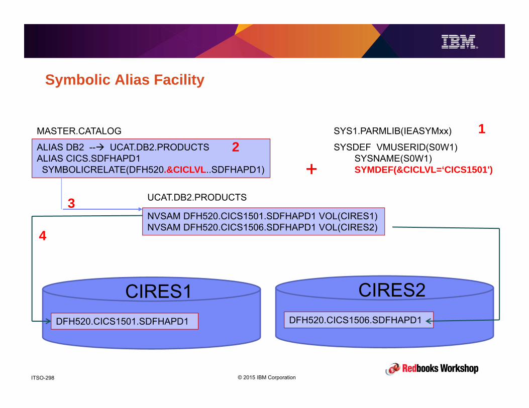
© 2015 IBM CorporationITSO-298
Symbolic Alias Facility
ALIAS DB2 -- UCAT.DB2.PRODUCTSALIAS CICS.SDFHAPD1SYMBOLICRELATE(DFH520.&CICLVL..SDFHAPD1)
NVSAM DFH520.CICS1501.SDFHAPD1 VOL(CIRES1)NVSAM DFH520.CICS1506.SDFHAPD1 VOL(CIRES2)
CIRES1DFH520.CICS1501.SDFHAPD1
CIRES2DFH520.CICS1506.SDFHAPD1
UCAT.DB2.PRODUCTS
MASTER.CATALOG
SYSDEF VMUSERID(S0W1) SYSNAME(S0W1) SYMDEF(&CICLVL=‘CICS1501')
SYS1.PARMLIB(IEASYMxx)
+
12
3
4
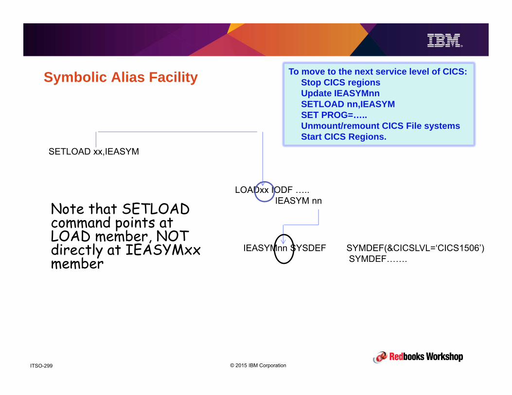
© 2015 IBM CorporationITSO-299
Symbolic Alias Facility
SETLOAD xx,IEASYM
LOADxx IODF …..IEASYM nn
IEASYMnn SYSDEF SYMDEF(&CICSLVL=‘CICS1506’)SYMDEF…….
Note that SETLOAD command points at LOAD member, NOT directly at IEASYMxx member
To move to the next service level of CICS:Stop CICS regionsUpdate IEASYMnnSETLOAD nn,IEASYMSET PROG=…..Unmount/remount CICS File systemsStart CICS Regions.
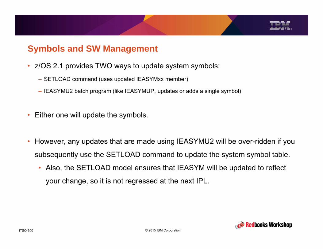
© 2015 IBM CorporationITSO-300
Symbols and SW Management
• z/OS 2.1 provides TWO ways to update system symbols:
– SETLOAD command (uses updated IEASYMxx member)
– IEASYMU2 batch program (like IEASYMUP, updates or adds a single symbol)
• Either one will update the symbols.
• However, any updates that are made using IEASYMU2 will be over-ridden if you
subsequently use the SETLOAD command to update the system symbol table.
• Also, the SETLOAD model ensures that IEASYM will be updated to reflect
your change, so it is not regressed at the next IPL.
© 2015 IBM CorporationITSO-301
Tip of the iceberg• This day only touched on a subset of the things you can do to make z/OS even more
cost effective. Many others are part of the operating system and just need to be
enabled, others are chargeable items, but can still significantly lower your costs
overall. Here are some things for you to think about:– Exploit large pages (requires you to specify an LFAREA value in Parmlib) and monitor the use of pageable
large pages.
– Exploit zIIPs and specify HONORPRIORITY=NO (unless you are using DB2 V11).
– Use System Managed Buffering for VSAM files.
– Use System Determined Blocksizes for Sequential data sets.
– Exploit latest level compilers, especially for CPU-intensive programs.
– Exploit appropriate capping functions and WLM policy optimization.
– Monitor for performance-related PTFs and apply as appropriate
• Finally, start planning NOW for the most effective way to configure your systems and
applications to enable you to get the best value from the new pricing options.
© 2015 IBM CorporationITSO-302
Thank You!
• Thank you for coming and for not shoring.
• Please fill out the evaluation forms and let us know if you have any questions or
suggestions.

2015 CPU MF Update
John Burg
August 13 2015
Session 17556
InsertCustomSessionQR ifDesired
© 2015 IBM Corporation
z Systems – WSC Performance Team
2
Agenda – CPU MF Counters Value of CPU MF Counters
– What, Why important for z13, and How to implement• z/OS 2.2 (and z/OS 2.1) HIS improvement
What’s New– zEC12 RNI– z13
• Display• Metrics and Formulas• Topology - SMF 99 Subtype 14s• WSC Tests
SMT-2 and SMT-1 Examples
Looking for z13 Volunteers
Summary

© 2015 IBM Corporation
z Systems – WSC Performance Team
3
Value of CPU Measurement Facility (CPU MF)
Recommended Methodology for successful z Systems ProcessorCapacity Planning
– Need on “Before” processor to determine LSPR workload
Validate achieved z Systems processor performance– Needed on “Before” and “After” processors
Provide insights for new features and functions– Continuously running on all LPARs
3
Capturing CPU MF data is an Industry “Best Practice”
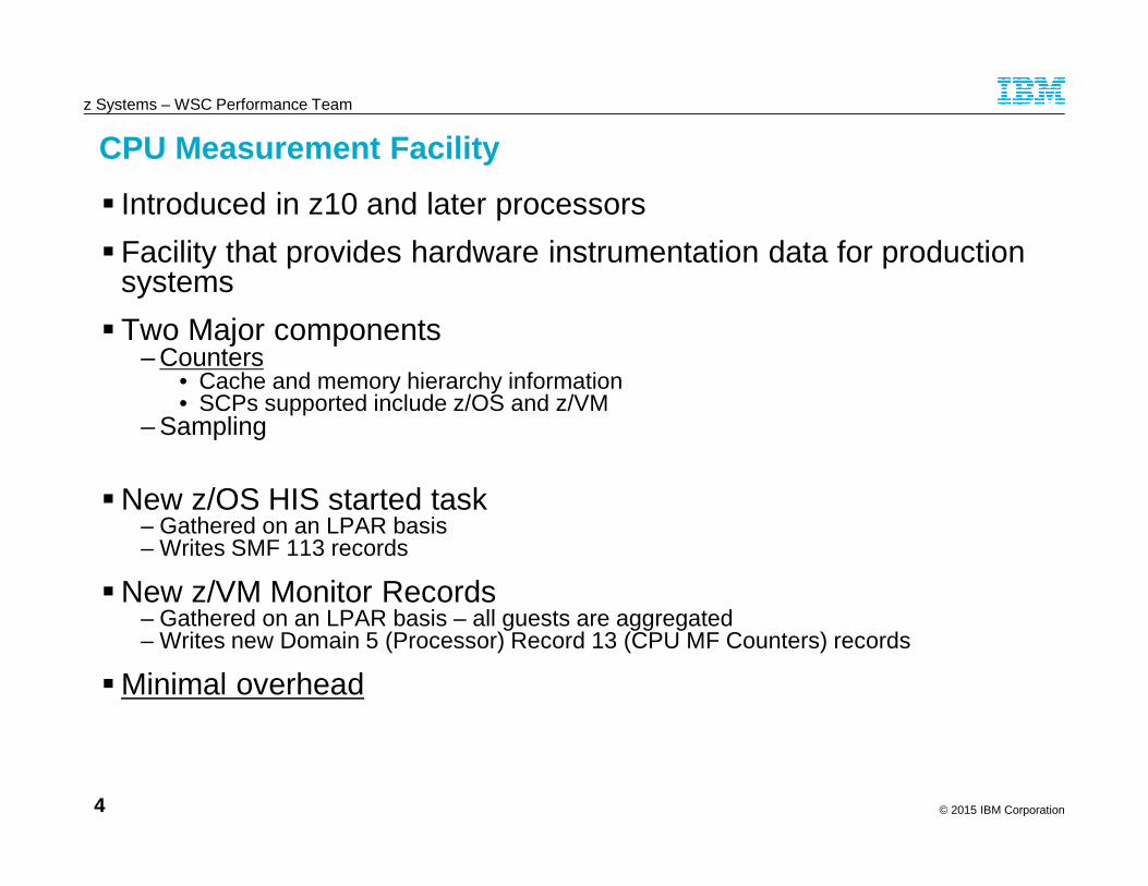
© 2015 IBM Corporation
z Systems – WSC Performance Team
4
CPU Measurement Facility
Introduced in z10 and later processors
Facility that provides hardware instrumentation data for productionsystems
Two Major components– Counters
• Cache and memory hierarchy information• SCPs supported include z/OS and z/VM
– SamplingInstruction time-in-CSECT
New z/OS HIS started task– Gathered on an LPAR basis– Writes SMF 113 records
New z/VM Monitor Records– Gathered on an LPAR basis – all guests are aggregated– Writes new Domain 5 (Processor) Record 13 (CPU MF Counters) records
Minimal overhead
4
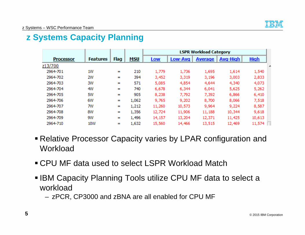
© 2015 IBM Corporation
z Systems – WSC Performance Team
5
z Systems Capacity Planning
Relative Processor Capacity varies by LPAR configuration andWorkload
CPU MF data used to select LSPR Workload Match
IBM Capacity Planning Tools utilize CPU MF data to select aworkload
– zPCR, CP3000 and zBNA are all enabled for CPU MF
5

© 2015 IBM Corporation
z Systems – WSC Performance Team
6
z13 Processor Performance
New Processor Design–Includes major pipeline enhancements and Larger Caches–1.10x (10%) average performance improvement at equal Nway vs
zEC12
Workload Variability–Workloads moving to z13 may see more variability than the last few
migrations–Potential Sources of Variability
• Workload interaction with Processor Design – may have variable butunpredictable benefit to IPC
• PR/SM placement of CPs and memory for an LPAR
6
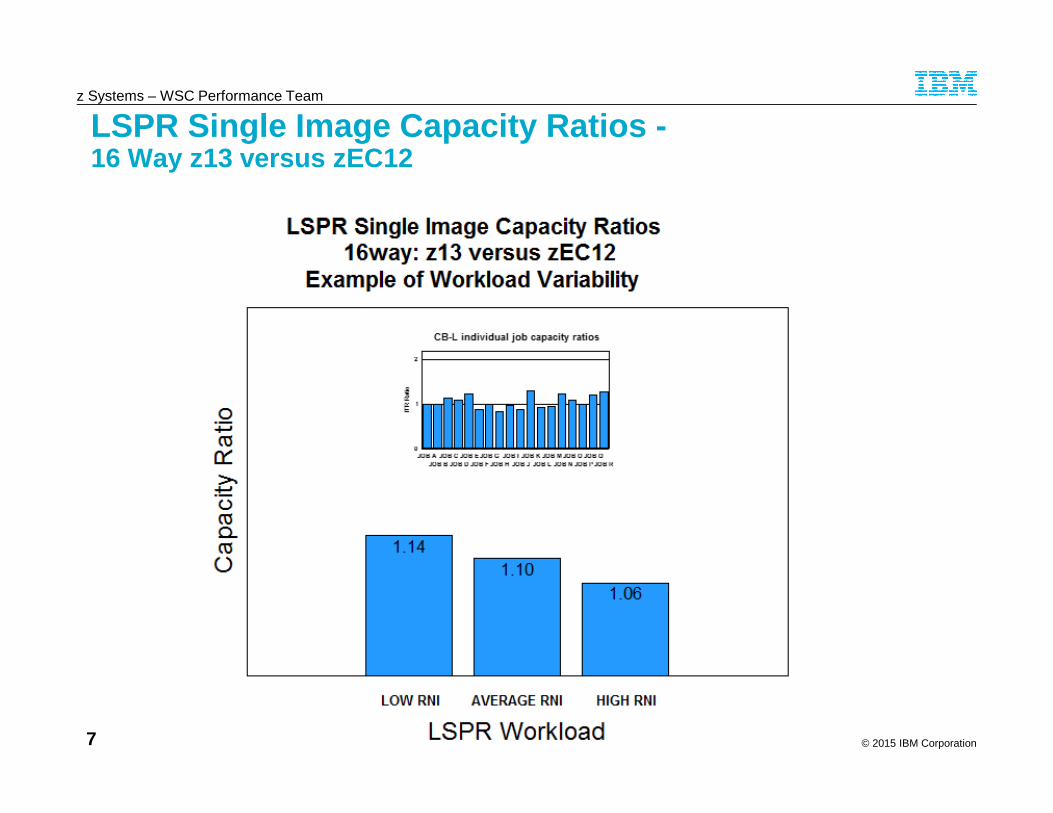
© 2015 IBM Corporation
z Systems – WSC Performance Team
7
LSPR Single Image Capacity Ratios -16 Way z13 versus zEC12
7

© 2015 IBM Corporation
z Systems – WSC Performance Team
8
Additional Customer Value with CPU MF Counters dataCounters can be used as a secondary source to:
– Supplement current performance data from SMF, RMF, DB2, CICS, etc.
– Help understand why performance may have changed
– Supported by many software products including Tivoli TDSz
Some examples of usage include:– Impact zEDC compression
– HiperDispatch Impact
– Configuration changes (Additional LPARs)
– 1 MB Page implementation
– Application Changes (e.g. CICS Threadsafe vs QR)
– Estimating Utilization Effect for capacity planning
– GHz change in Power Saving Mode
– Crypto CPACF usage
8
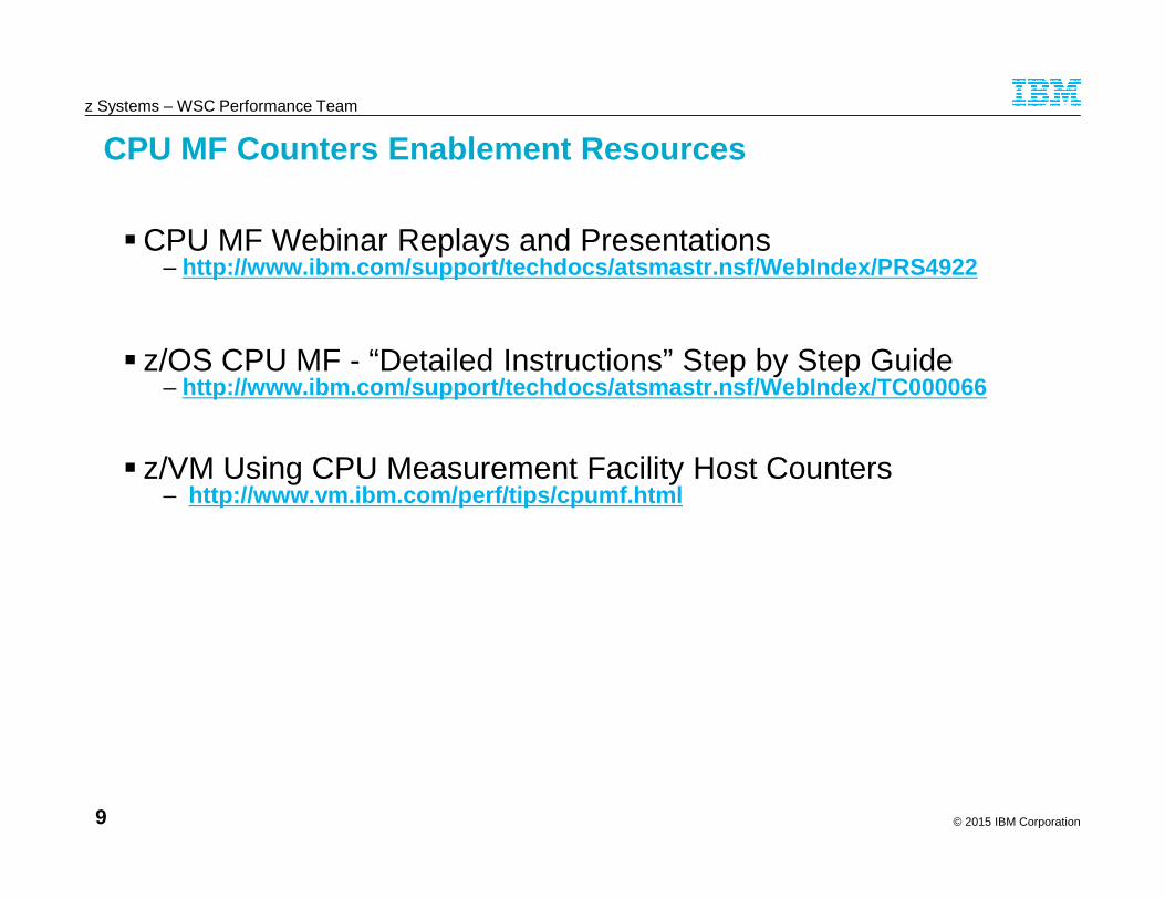
© 2015 IBM Corporation
z Systems – WSC Performance Team
9
CPU MF Counters Enablement Resources
CPU MF Webinar Replays and Presentations– http://www.ibm.com/support/techdocs/atsmastr.nsf/WebIndex/PRS4922
z/OS CPU MF - “Detailed Instructions” Step by Step Guide– http://www.ibm.com/support/techdocs/atsmastr.nsf/WebIndex/TC000066
z/VM Using CPU Measurement Facility Host Counters– http://www.vm.ibm.com/perf/tips/cpumf.html
9
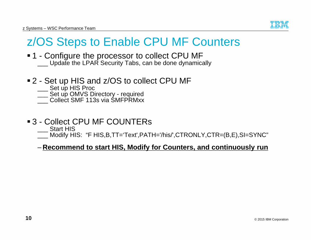
© 2015 IBM Corporation
z Systems – WSC Performance Team
10
z/OS Steps to Enable CPU MF Counters 1 - Configure the processor to collect CPU MF
___ Update the LPAR Security Tabs, can be done dynamically
2 - Set up HIS and z/OS to collect CPU MF___ Set up HIS Proc___ Set up OMVS Directory - required___ Collect SMF 113s via SMFPRMxx
3 - Collect CPU MF COUNTERs___ Start HIS___ Modify HIS: “F HIS,B,TT=‘Text',PATH='/his/',CTRONLY,CTR=(B,E),SI=SYNC”
– Recommend to start HIS, Modify for Counters, and continuously run
10
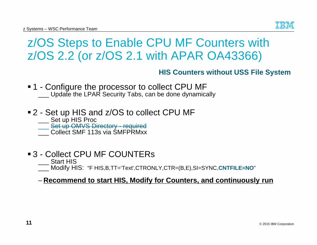
© 2015 IBM Corporation
z Systems – WSC Performance Team
11
z/OS Steps to Enable CPU MF Counters withz/OS 2.2 (or z/OS 2.1 with APAR OA43366)
1 - Configure the processor to collect CPU MF___ Update the LPAR Security Tabs, can be done dynamically
2 - Set up HIS and z/OS to collect CPU MF___ Set up HIS Proc___ Set up OMVS Directory - required___ Collect SMF 113s via SMFPRMxx
3 - Collect CPU MF COUNTERs___ Start HIS___ Modify HIS: “F HIS,B,TT=‘Text',CTRONLY,CTR=(B,E),SI=SYNC,CNTFILE=NO”
– Recommend to start HIS, Modify for Counters, and continuously run
11
HIS Counters without USS File System

© 2015 IBM Corporation
z Systems – WSC Performance Team
12
SMF 113s Space Requirements Are Minimal
The SMF 113 record puts minimal pressure on SMF– 452 bytes for each logical processor per interval
Example below is from 3 z196s processors• 713, 716 and 718• 10 Systems• 5 Days, 24 hours
SMF 113s were 1.2% of the space compared to SMF 70s & 72s
12
RECORD RECORDS PERCENT AVG. RECORD MIN. RECORD MAX. RECORD RECORDS
Total Size (with
AVG. Record Size)
% Total Size (with
AVG. Record Size)
TYPE READ OF TOTAL LENGTH LENGTH LENGTH WRITTEN70 14,250 1.8% 14,236 640 32,736 14,250 202,865,850 15.1%72 744,014 93.5% 1,516 1,104 20,316 744,014 1,128,252,590 83.7%
113 37,098 4.7% 452 452 452 37,098 16,768,296 1.2%
TOTAL 795,362 100.0% 1,695 18 32,736 795,362 1,347,886,736 100.0%

© 2015 IBM Corporation
z Systems – WSC Performance Team
14
Processor Measurement Methodology
zPCR provides overall processor capacity expectations
Variations within workload is expected– An individual job can see a shortfall but the measurement is for the entire
workload
Take care with customer synthetic benchmarks as they are oftensubject to significant measurement error
See “Processor Migration Capacity Analysis in a ProductionEnvironment ”
– http://www.ibm.com/support/techdocs/atsmastr.nsf/WebIndex/WP100744
14 JOB AJOB B
JOB CJOB D
JOB EJOB F
JOB GJOB H
JOB IJOB J
JOB KJOB L
JOB MJOB N
JOB OJOB P
JOB QJOB R
0
1
2
ITR
Ra
tio
CB-L individual job capacity ratios

© 2015 IBM Corporation
z Systems – WSC Performance Team
1515
CPU MF Update
zEC12 and z13

© 2015 IBM Corporation
z Systems – WSC Performance Team
16
CPU MF – What’s New for z13? Updated zEC12 RNI
Same LSPR RNI Workload Decision Table
Same Metrics as previous processors–New formulas
New “Miss” cycles measurement allows improved Metrics:–CPI = Instruction Complexity CPI + Finite Cache CPI–Estimated Sourcing Cycles per L1 Miss
SMF 99s Subtype 14–Drawer, Node, Chip identification for Logical Processor (thread)
CPU MF Metrics at Logical Processor or Thread level–SMT 1 Logical Processor level–SMT 2 Thread level
16
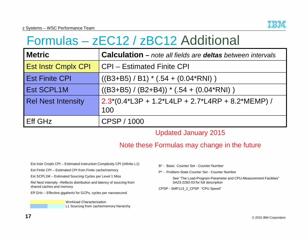
© 2015 IBM Corporation
z Systems – WSC Performance Team
17 17
Formulas – zEC12 / zBC12 AdditionalMetric Calculation – note all fields are deltas between intervals
Est Instr Cmplx CPI CPI – Estimated Finite CPI
Est Finite CPI ((B3+B5) / B1) * (.54 + (0.04*RNI) )
Est SCPL1M ((B3+B5) / (B2+B4)) * (.54 + (0.04*RNI) )
Rel Nest Intensity 2.3*(0.4*L3P + 1.2*L4LP + 2.7*L4RP + 8.2*MEMP) /100
Eff GHz CPSP / 1000
Updated January 2015
Note these Formulas may change in the future
Est Instr Cmplx CPI – Estimated Instruction Complexity CPI (infinite L1)
Est Finite CPI – Estimated CPI from Finite cache/memory
Est SCPL1M – Estimated Sourcing Cycles per Level 1 Miss
Rel Nest Intensity –Reflects distribution and latency of sourcing fromshared caches and memory
Eff GHz – Effective gigahertz for GCPs, cycles per nanosecond
Workload CharacterizationL1 Sourcing from cache/memory hierarchy
B* - Basic Counter Set - Counter Number
P* - Problem-State Counter Set - Counter Number
See “The Load-Program-Parameter and CPU-Measurement Facilities”SA23-2260-03 for full description
CPSP - SMF113_2_CPSP “CPU Speed”

© 2015 IBM Corporation
z Systems – WSC Performance Team
18
Current table applies to z10 EC, z10 BC, z196, z114,zEC12, zBC12 and z13 CPU MF data
L1MP RNI LSPR Workload Match
< 3%>= 0.75< 0.75
AVERAGELOW
3% to 6%>1.0
0.6 to 1.0< 0.6
HIGHAVERAGELOW
> 6%>= 0.75< 0.75
HIGHAVERAGE
RNI-based LSPR Workload Decision Table

© 2015 IBM Corporation
z Systems – WSC Performance Team
19
z13 Metrics

© 2015 IBM Corporation
z Systems – WSC Performance Team
20
IBM z13 versus zEC12 Hardware Comparison
...
Memory
L4 Cache
L2
CPU1
L1
L3 Cache
L2
CPU6
L1... L2
CPU1
L1
L3 Cache
L2
CPU6
L1...
...
Memory
L4 Cache
L2
PU1
L1
L3 Cache
... L2
PU8
L1
L2
PU1
L1
L3 Cache
...L2
PU8
L1
...
Memory
L4 Cache
L2
PU1
L1
L3 Cache
... L2
PU8
L1
L2
PU1
L1
L3 Cache
...L2
PU8
L1
zEC12
– CPU• 5.5 GHz
• Enhanced Out-Of-Order
– Caches• L1 private 64k i, 96k d
• L2 private 1 MB i + 1 MB d
• L3 shared 48 MB / chip
• L4 shared 384 MB / book
z13
– CPU• 5.0 GHz
• Major pipeline enhancements
– Caches• L1 private 96k i, 128k d
• L2 private 2 MB i + 2 MB d
• L3 shared 64 MB / chip
• L4 shared 480 MB / node
- plus 224 MB L3 NIC Directory
Single Book View
Single Drawer View - Two Nodes
Node 1 Node 2

© 2015 IBM Corporation
z Systems – WSC Performance Team
21 21
z/OS SMF 113 Record
SMF113_2_CTRVN2–“1” = z10 EC/BC–“2” = z196 / z114–“3” = zEC12 / zBC12–“4” = z13

© 2015 IBM Corporation
z Systems – WSC Performance Team
22
Operations – Display HIS Command on z13
z13 “4”
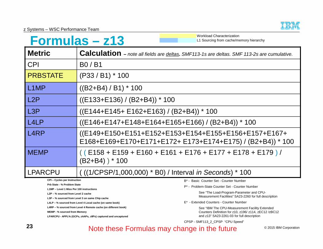
© 2015 IBM Corporation
z Systems – WSC Performance Team
23 23
Formulas – z13Metric Calculation – note all fields are deltas. SMF113-1s are deltas. SMF 113-2s are cumulative.
CPI B0 / B1
PRBSTATE (P33 / B1) * 100
L1MP ((B2+B4) / B1) * 100
L2P ((E133+E136) / (B2+B4)) * 100
L3P ((E144+E145+ E162+E163) / (B2+B4)) * 100
L4LP ((E146+E147+E148+E164+E165+E166) / (B2+B4)) * 100
L4RP ((E149+E150+E151+E152+E153+E154+E155+E156+E157+E167+E168+E169+E170+E171+E172+ E173+E174+E175) / (B2+B4)) * 100
MEMP ( ( E158 + E159 + E160 + E161 + E176 + E177 + E178 + E179 ) /(B2+B4) ) * 100
LPARCPU ( ((1/CPSP/1,000,000) * B0) / Interval in Seconds) * 100
Workload CharacterizationL1 Sourcing from cache/memory hierarchy
CPI – Cycles per Instruction
Prb State - % Problem State
L1MP – Level 1 Miss Per 100 instructions
L2P – % sourced from Level 2 cache
L3P – % sourced from Level 3 on same Chip cache
L4LP – % sourced from Level 4 Local cache (on same book)
L4RP – % sourced from Level 4 Remote cache (on different book)
MEMP - % sourced from Memory
LPARCPU - APPL% (GCPs, zAAPs, zIIPs) captured and uncaptured
Note these Formulas may change in the future
B* - Basic Counter Set - Counter Number
P* - Problem-State Counter Set - Counter Number
See “The Load-Program-Parameter and CPU-Measurement Facilities” SA23-2260 for full description
E* - Extended Counters - Counter Number
See “IBM The CPU-Measurement Facility ExtendedCounters Definition for z10, z196/ z114, zEC12 /zBC12and z13” SA23-2261-03 for full description
CPSP - SMF113_2_CPSP “CPU Speed”

© 2015 IBM Corporation
z Systems – WSC Performance Team
24 24
Formulas – z13 AdditionalMetric Calculation– note all fields are deltas. SMF113-1s are deltas. SMF 113-2s are
cumulative.
Est Instr Cmplx CPI CPI – Estimated Finite CPI
Est Finite CPI E143 / B1
Est SCPL1M E143 / (B2+B4)
Rel Nest Intensity 2.6*(0.4*L3P + 1.6*L4LP + 3.5*L4RP + 7.5*MEMP) / 100
Eff GHz CPSP / 1000
Note these Formulas may change in the future
Est Instr Cmplx CPI – Estimated Instruction Complexity CPI (infinite L1)
Est Finite CPI – Estimated CPI from Finite cache/memory
Est SCPL1M – Estimated Sourcing Cycles per Level 1 Miss
Rel Nest Intensity –Reflects distribution and latency of sourcing fromshared caches and memory
Eff GHz – Effective gigahertz for GCPs, cycles per nanosecond
Workload CharacterizationL1 Sourcing from cache/memory hierarchy
B* - Basic Counter Set - Counter Number
P* - Problem-State Counter Set - Counter Number
See “The Load-Program-Parameter and CPU-Measurement Facilities” SA23-2260 for full description
E* - Extended Counters - Counter Number
See “IBM The CPU-Measurement Facility ExtendedCounters Definition for z10, z196/ z114, zEC12 /zBC12and z13” SA23-2261-03 for full description
CPSP - SMF113_2_CPSP “CPU Speed”
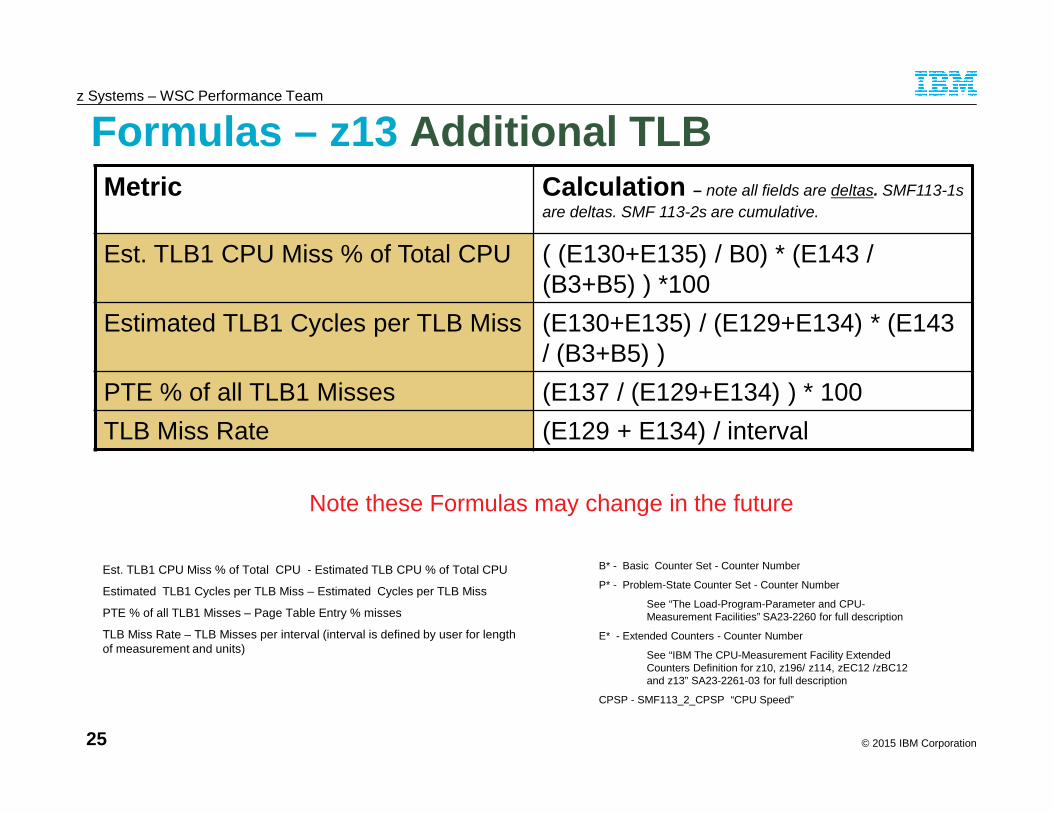
© 2015 IBM Corporation
z Systems – WSC Performance Team
25 25
Formulas – z13 Additional TLBMetric Calculation – note all fields are deltas. SMF113-1s
are deltas. SMF 113-2s are cumulative.
Est. TLB1 CPU Miss % of Total CPU ( (E130+E135) / B0) * (E143 /(B3+B5) ) *100
Estimated TLB1 Cycles per TLB Miss (E130+E135) / (E129+E134) * (E143/ (B3+B5) )
PTE % of all TLB1 Misses (E137 / (E129+E134) ) * 100
TLB Miss Rate (E129 + E134) / interval
Note these Formulas may change in the future
Est. TLB1 CPU Miss % of Total CPU - Estimated TLB CPU % of Total CPU
Estimated TLB1 Cycles per TLB Miss – Estimated Cycles per TLB Miss
PTE % of all TLB1 Misses – Page Table Entry % misses
TLB Miss Rate – TLB Misses per interval (interval is defined by user for lengthof measurement and units)
B* - Basic Counter Set - Counter Number
P* - Problem-State Counter Set - Counter Number
See “The Load-Program-Parameter and CPU-Measurement Facilities” SA23-2260 for full description
E* - Extended Counters - Counter Number
See “IBM The CPU-Measurement Facility ExtendedCounters Definition for z10, z196/ z114, zEC12 /zBC12and z13” SA23-2261-03 for full description
CPSP - SMF113_2_CPSP “CPU Speed”
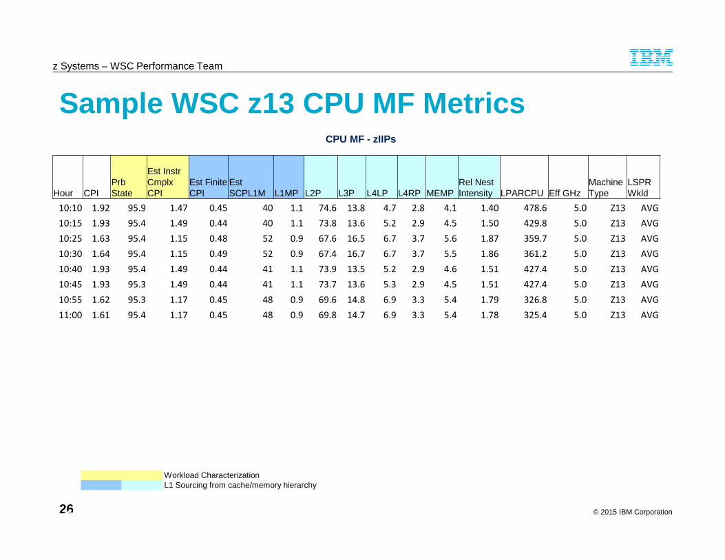
© 2015 IBM Corporation
z Systems – WSC Performance Team
2626
Sample WSC z13 CPU MF Metrics
Workload CharacterizationL1 Sourcing from cache/memory hierarchy
CPU MF - zIIPs
Hour CPIPrbState
Est InstrCmplxCPI
Est FiniteCPI
EstSCPL1M L1MP L2P L3P L4LP L4RP MEMP
Rel NestIntensity LPARCPU Eff GHz
MachineType
LSPRWkld
10:10 1.92 95.9 1.47 0.45 40 1.1 74.6 13.8 4.7 2.8 4.1 1.40 478.6 5.0 Z13 AVG
10:15 1.93 95.4 1.49 0.44 40 1.1 73.8 13.6 5.2 2.9 4.5 1.50 429.8 5.0 Z13 AVG
10:25 1.63 95.4 1.15 0.48 52 0.9 67.6 16.5 6.7 3.7 5.6 1.87 359.7 5.0 Z13 AVG
10:30 1.64 95.4 1.15 0.49 52 0.9 67.4 16.7 6.7 3.7 5.5 1.86 361.2 5.0 Z13 AVG
10:40 1.93 95.4 1.49 0.44 41 1.1 73.9 13.5 5.2 2.9 4.6 1.51 427.4 5.0 Z13 AVG
10:45 1.93 95.3 1.49 0.44 41 1.1 73.7 13.6 5.3 2.9 4.5 1.51 427.4 5.0 Z13 AVG
10:55 1.62 95.3 1.17 0.45 48 0.9 69.6 14.8 6.9 3.3 5.4 1.79 326.8 5.0 Z13 AVG
11:00 1.61 95.4 1.17 0.45 48 0.9 69.8 14.7 6.9 3.3 5.4 1.78 325.4 5.0 Z13 AVG

© 2015 IBM Corporation
z Systems – WSC Performance Team
27
SMF 99s (subtype 14)
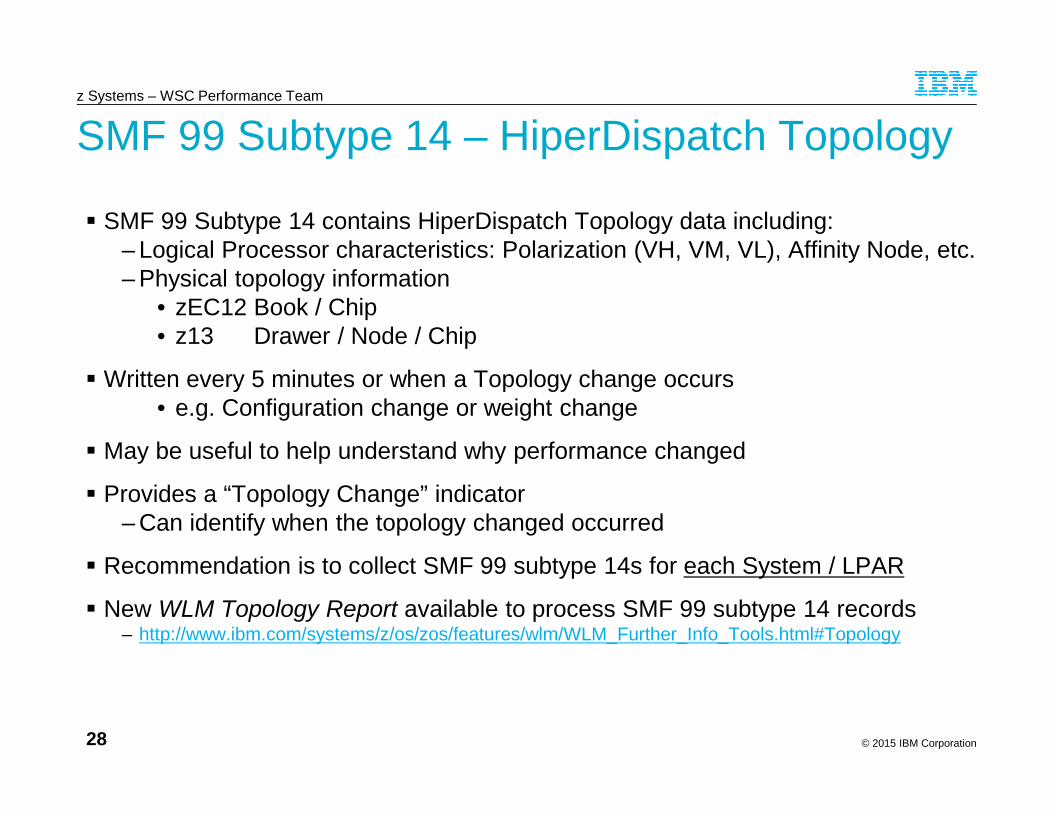
© 2015 IBM Corporation
z Systems – WSC Performance Team
28
SMF 99 Subtype 14 – HiperDispatch Topology
SMF 99 Subtype 14 contains HiperDispatch Topology data including:– Logical Processor characteristics: Polarization (VH, VM, VL), Affinity Node, etc.– Physical topology information
• zEC12 Book / Chip• z13 Drawer / Node / Chip
Written every 5 minutes or when a Topology change occurs• e.g. Configuration change or weight change
May be useful to help understand why performance changed
Provides a “Topology Change” indicator– Can identify when the topology changed occurred
Recommendation is to collect SMF 99 subtype 14s for each System / LPAR
New WLM Topology Report available to process SMF 99 subtype 14 records– http://www.ibm.com/systems/z/os/zos/features/wlm/WLM_Further_Info_Tools.html#Topology

© 2015 IBM Corporation
z Systems – WSC Performance Team
29
z13 SYSD Topology – Jan 30
Topology for 14:20 - 14:40 SYSD TestsChanged at 14:11:42. Due toadding zIIPs on SYSB
Topology before SYSD Tests
© 2015 IBM Corporation
z Systems – WSC Performance Team
30
z13 SMT Capacity and Performance Metrics

© 2015 IBM Corporation
z Systems – WSC Performance Team
31
WSC z13 zIIP SMT Test z13-736 N96 with 12 zIIPs
–Processor at pre GA code level–Tests ran on partition SYSD / USP02 defined with 6 GCPs and 5 zIIPs
• 5 zIIPS: 2 VH, 2 VM and 1 VL–Other partitions running very limited load, SYSD weights not enforced–z/OS 2.1
External Server driving 2 Java 8 workloads–Gets memory and calculates PI to 6 digits (CB_MED)–Creates a 25 page PDF document (CB_LOW)–Artificial driver to drive large number of transactions in 5 minute interval–SMF set to 5 minute intervals–SMT vs Non-SMT with IIPHONORPRIORITY=YES and NO
Objective–Utilize ~58% 5 Logical zIIPs and ~25% 12 Physical zIIPs–Review response times and zIIP utilization with non-SMT and SMT
These numbers come from a synthetic Benchmark and donot represent a production workload
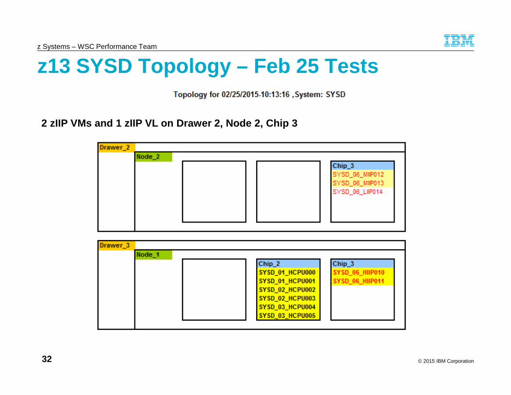
© 2015 IBM Corporation
z Systems – WSC Performance Team
32
z13 SYSD Topology – Feb 25 Tests
2 zIIP VMs and 1 zIIP VL on Drawer 2, Node 2, Chip 3

© 2015 IBM Corporation
z Systems – WSC Performance Team
33
WSC z13 zIIP SMT Test Summary
IIPHonorPriority=YESIIPHonorPriority=NO
2 threads 2 threads1 thread 1 thread
These numbers come from a synthetic Benchmark and donot represent a production workload
SMT-2 Mode resulted in• Lower zIIP Utilization• CB_MED Higher Response times

© 2015 IBM Corporation
z Systems – WSC Performance Team
34
WSC z13 zIIP SMT Test Summary – CPU MF
These numbers come from a synthetic Benchmark and donot represent a production workload
CPU MF – zIIP Pool
RMFStart SMT TDEN CPI Prb State
Est InstrCmplx CPI
EstFiniteCPI
EstSCPL1M L1MP L2P L3P L4LP L4RP MEMP
Rel NestIntensity LPARCPU Eff GHz
MachineType
LSPRWkld
10:10 2 1.79 1.92 95.9 1.47 0.45 40 1.1 74.6 13.8 4.7 2.8 4.1 1.40 478.6 5.0 Z13 AVG
10:15 2 1.75 1.93 95.4 1.49 0.44 40 1.1 73.8 13.6 5.2 2.9 4.5 1.50 429.8 5.0 Z13 AVG
10:25 1 1.00 1.63 95.4 1.15 0.48 52 0.9 67.6 16.5 6.7 3.7 5.6 1.87 359.7 5.0 Z13 AVG
10:30 1 1.00 1.64 95.4 1.15 0.49 52 0.9 67.4 16.7 6.7 3.7 5.5 1.86 361.2 5.0 Z13 AVG
10:40 2 1.74 1.93 95.4 1.49 0.44 41 1.1 73.9 13.5 5.2 2.9 4.6 1.51 427.4 5.0 Z13 AVG
10:45 2 1.74 1.93 95.3 1.49 0.44 41 1.1 73.7 13.6 5.3 2.9 4.5 1.51 427.4 5.0 Z13 AVG
10:55 1 1.00 1.62 95.3 1.17 0.45 48 0.9 69.6 14.8 6.9 3.3 5.4 1.79 326.8 5.0 Z13 AVG
11:00 1 1.00 1.61 95.4 1.17 0.45 48 0.9 69.8 14.7 6.9 3.3 5.4 1.78 325.4 5.0 Z13 AVG
SMT-1 has a lower CPI (faster) than SMT-2

© 2015 IBM Corporation
z Systems – WSC Performance Team
35
SYSD RMF CPU Activity – zIIPs Feb 25 10:45 AM
Max Capacity Factor (MAX CF) – How much work a core can complete (rate of delivery)Capacity Factor (CF) – How much work a core actually completes (rate of delivery)Average Thread Density (AVG TD) – Average executing threads during Core BusyMT % Productivity (PROD) – Core Busy Time Effectiveness (Capacity in use / Capacity max)MT % Utilization (UTIL) – Core Busy Time / Core Available Time
Core Thread Core
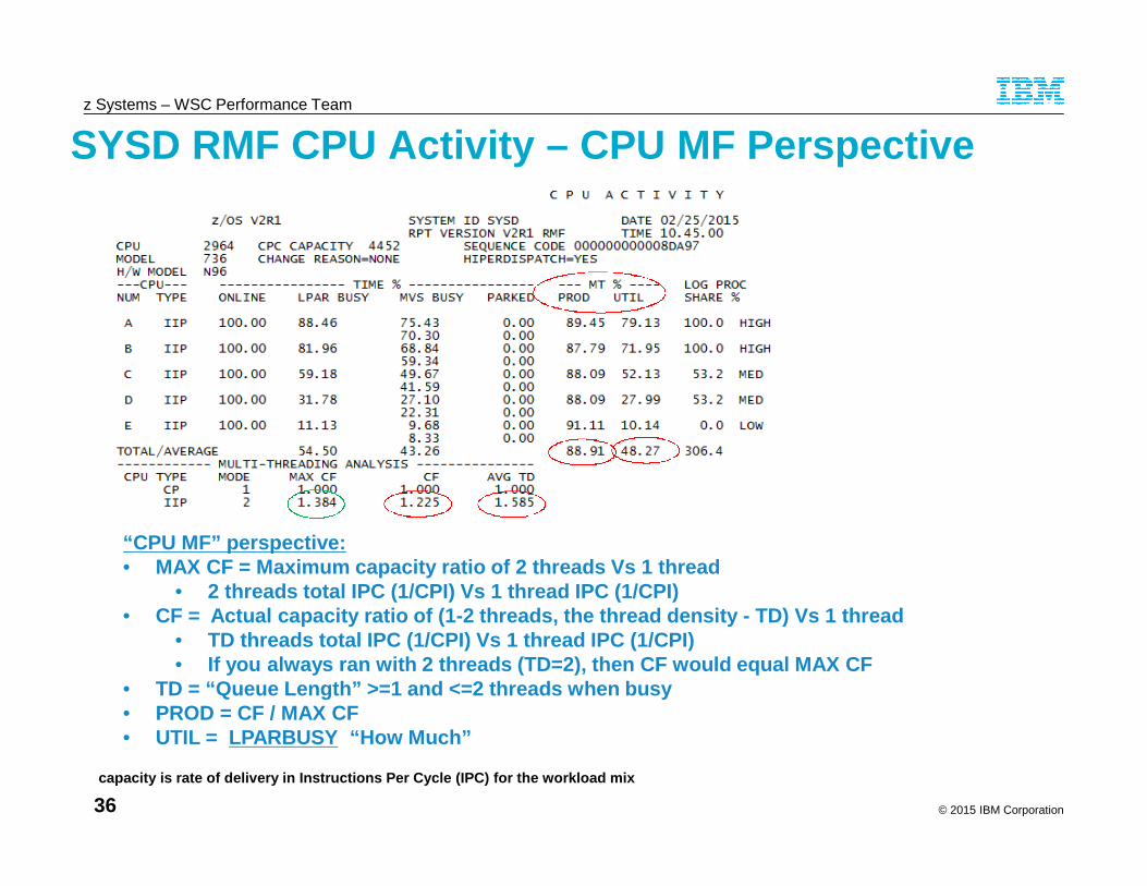
© 2015 IBM Corporation
z Systems – WSC Performance Team
36
SYSD RMF CPU Activity – CPU MF Perspective
“CPU MF” perspective:• MAX CF = Maximum capacity ratio of 2 threads Vs 1 thread
• 2 threads total IPC (1/CPI) Vs 1 thread IPC (1/CPI)• CF = Actual capacity ratio of (1-2 threads, the thread density - TD) Vs 1 thread
• TD threads total IPC (1/CPI) Vs 1 thread IPC (1/CPI)• If you always ran with 2 threads (TD=2), then CF would equal MAX CF
• TD = “Queue Length” >=1 and <=2 threads when busy• PROD = CF / MAX CF• UTIL = LPARBUSY “How Much”
capacity is rate of delivery in Instructions Per Cycle (IPC) for the workload mix

© 2015 IBM Corporation
z Systems – WSC Performance Team
37
SYSD RMF CPU Activity – CPU MF Perspective
“MAX CF” estimate from a CPU MF perspective• If CPI MT-1 = 1.61, then IPC are 1 / 1.61 = .6211• If CPI MT-2 = 2.33, then IPC are 1 / 2.33 = .4298• MAX CF = (2 threads x .4298) / .6211 = 1.384
capacity is rate of delivery in Instructions Per Cycle (IPC) for the workload mix

© 2015 IBM Corporation
z Systems – WSC Performance Team
38
SYSD CPU MF Thread Metrics – zIIPs Feb 25 10:45 AM
CPU MF - zIIPs
RMFStart SMT CPID THREAD CPI Prb State
Est InstrCmplxCPI
EstFiniteCPI
EstSCPL1M L1MP L2P L3P L4LP L4RP MEMP
Rel NestIntensity LPARCPU Eff GHz
MachineType
LSPRWkld Drawer Node Chip Logical
10:45 2 20 0 1.90 95.3 1.49 0.41 38 1.1 74.0 13.3 4.9 3.1 4.7 1.54 74.6 5.0 Z13 AVG 3 1 3 VH
10:45 2 21 1 2.03 94.9 1.60 0.43 38 1.1 73.9 13.3 4.9 3.1 4.8 1.57 69.5 5.0 Z13 AVG 3 1 3 VH
10:45 2 22 0 1.81 95.6 1.42 0.39 37 1.0 74.0 13.5 4.9 3.1 4.6 1.51 68.1 5.0 Z13 AVG 3 1 3 VH
10:45 2 23 1 1.99 94.9 1.56 0.43 38 1.1 73.8 13.6 4.9 3.1 4.6 1.53 58.7 5.0 Z13 AVG 3 1 3 VH
10:45 2 24 0 1.84 95.7 1.38 0.46 45 1.0 73.9 13.3 5.9 2.6 4.3 1.46 49.0 5.0 Z13 AVG 2 2 3 VM
10:45 2 25 1 2.08 95.0 1.58 0.50 45 1.1 73.6 13.6 5.9 2.5 4.4 1.48 41.0 5.0 Z13 AVG 2 2 3 VM
10:45 2 26 0 1.84 95.8 1.37 0.47 46 1.0 72.9 14.5 5.9 2.6 4.1 1.44 26.7 5.0 Z13 AVG 2 2 3 VM
10:45 2 27 1 2.05 95.2 1.54 0.51 46 1.1 72.8 14.6 5.8 2.6 4.3 1.46 22.0 5.0 Z13 AVG 2 2 3 VM
10:45 2 28 0 1.83 96.1 1.33 0.50 49 1.0 71.5 16.0 5.6 3.0 4.0 1.45 9.6 5.0 Z13 AVG 2 2 3 VL
10:45 2 29 1 2.07 95.5 1.51 0.56 51 1.1 71.1 15.9 5.8 3.0 4.2 1.50 8.2 5.0 Z13 AVG 2 2 3 VL
Total 1.93 95.3 1.49 0.44 41 1.1 73.7 13.6 5.3 2.9 4.5 1.51 427.4 5.0 Z13 AVG
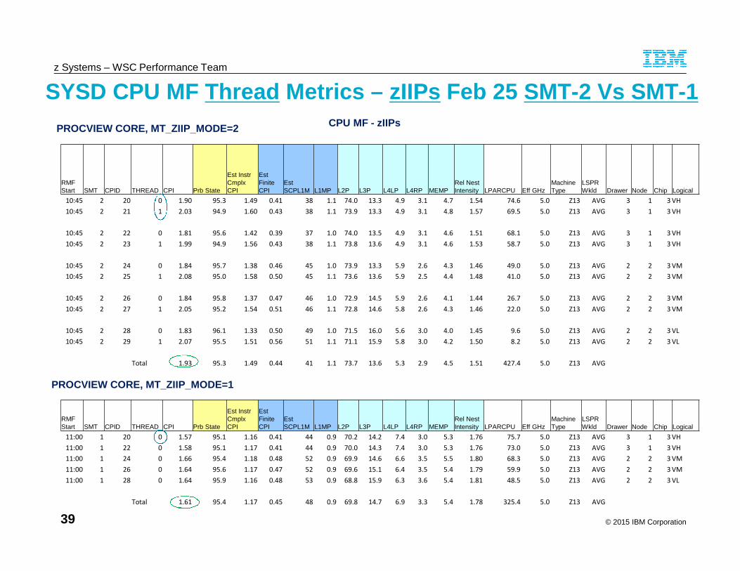
© 2015 IBM Corporation
z Systems – WSC Performance Team
39
SYSD CPU MF Thread Metrics – zIIPs Feb 25 SMT-2 Vs SMT-1CPU MF - zIIPsPROCVIEW CORE, MT_ZIIP_MODE=2
RMFStart SMT CPID THREAD CPI Prb State
Est InstrCmplxCPI
EstFiniteCPI
EstSCPL1M L1MP L2P L3P L4LP L4RP MEMP
Rel NestIntensity LPARCPU Eff GHz
MachineType
LSPRWkld Drawer Node Chip Logical
10:45 2 20 0 1.90 95.3 1.49 0.41 38 1.1 74.0 13.3 4.9 3.1 4.7 1.54 74.6 5.0 Z13 AVG 3 1 3 VH
10:45 2 21 1 2.03 94.9 1.60 0.43 38 1.1 73.9 13.3 4.9 3.1 4.8 1.57 69.5 5.0 Z13 AVG 3 1 3 VH
10:45 2 22 0 1.81 95.6 1.42 0.39 37 1.0 74.0 13.5 4.9 3.1 4.6 1.51 68.1 5.0 Z13 AVG 3 1 3 VH
10:45 2 23 1 1.99 94.9 1.56 0.43 38 1.1 73.8 13.6 4.9 3.1 4.6 1.53 58.7 5.0 Z13 AVG 3 1 3 VH
10:45 2 24 0 1.84 95.7 1.38 0.46 45 1.0 73.9 13.3 5.9 2.6 4.3 1.46 49.0 5.0 Z13 AVG 2 2 3 VM
10:45 2 25 1 2.08 95.0 1.58 0.50 45 1.1 73.6 13.6 5.9 2.5 4.4 1.48 41.0 5.0 Z13 AVG 2 2 3 VM
10:45 2 26 0 1.84 95.8 1.37 0.47 46 1.0 72.9 14.5 5.9 2.6 4.1 1.44 26.7 5.0 Z13 AVG 2 2 3 VM
10:45 2 27 1 2.05 95.2 1.54 0.51 46 1.1 72.8 14.6 5.8 2.6 4.3 1.46 22.0 5.0 Z13 AVG 2 2 3 VM
10:45 2 28 0 1.83 96.1 1.33 0.50 49 1.0 71.5 16.0 5.6 3.0 4.0 1.45 9.6 5.0 Z13 AVG 2 2 3 VL
10:45 2 29 1 2.07 95.5 1.51 0.56 51 1.1 71.1 15.9 5.8 3.0 4.2 1.50 8.2 5.0 Z13 AVG 2 2 3 VL
Total 1.93 95.3 1.49 0.44 41 1.1 73.7 13.6 5.3 2.9 4.5 1.51 427.4 5.0 Z13 AVG
RMFStart SMT CPID THREAD CPI Prb State
Est InstrCmplxCPI
EstFiniteCPI
EstSCPL1M L1MP L2P L3P L4LP L4RP MEMP
Rel NestIntensity LPARCPU Eff GHz
MachineType
LSPRWkld Drawer Node Chip Logical
11:00 1 20 0 1.57 95.1 1.16 0.41 44 0.9 70.2 14.2 7.4 3.0 5.3 1.76 75.7 5.0 Z13 AVG 3 1 3 VH
11:00 1 22 0 1.58 95.1 1.17 0.41 44 0.9 70.0 14.3 7.4 3.0 5.3 1.76 73.0 5.0 Z13 AVG 3 1 3 VH
11:00 1 24 0 1.66 95.4 1.18 0.48 52 0.9 69.9 14.6 6.6 3.5 5.5 1.80 68.3 5.0 Z13 AVG 2 2 3 VM
11:00 1 26 0 1.64 95.6 1.17 0.47 52 0.9 69.6 15.1 6.4 3.5 5.4 1.79 59.9 5.0 Z13 AVG 2 2 3 VM
11:00 1 28 0 1.64 95.9 1.16 0.48 53 0.9 68.8 15.9 6.3 3.6 5.4 1.81 48.5 5.0 Z13 AVG 2 2 3 VL
Total 1.61 95.4 1.17 0.45 48 0.9 69.8 14.7 6.9 3.3 5.4 1.78 325.4 5.0 Z13 AVG
PROCVIEW CORE, MT_ZIIP_MODE=1

© 2015 IBM Corporation
z Systems – WSC Performance Team
40
Looking for z13 Migration “Volunteers” to send SMF dataWant to validate / refine Workload selection metrics
Looking for “Volunteers”
(3 days, 24 hours/day, SMF 70s, 71s, 72s, 99 subtype 14s,113s per LPAR)
“Before z196 / zEC12” and “After z13”
Production partitions preferred
If interested send note to [email protected],
No deliverable will be returned
Benefit: Opportunity to ensure your data is used to influence analysis

© 2015 IBM Corporation
z Systems – WSC Performance Team
41
CPU MF Summary
CPU MF Counters provide better information for moresuccessful capacity planning
Same data used to validate the LSPR workloads can nowbe obtained from production systems
CPU MF Counters can also be useful for performanceanalysis
Enable CPU MF Counters Today!– Continuously collect SMF 113s for all your systems

© 2015 IBM Corporation
z Systems – WSC Performance Team
42
Thank You forAttending!

© 2015 IBM Corporation
z Systems – WSC Performance Team
43
Trademarks
The following are trademarks of the International Business Machines Corporation in the United States, other countries, or both.
The following are trademarks or registered trademarks of other companies.
* All other products may be trademarks or registered trademarks of their respective companies.
Notes:Performance is in Internal Throughput Rate (ITR) ratio based on measurements and projections using standard IBM benchmarks in a controlled environment. The actual throughput that anyuser will experience will vary depending upon considerations such as the amount of multiprogramming in the user's job stream, the I/O configuration, the storage configuration, and theworkload processed. Therefore, no assurance can be given that an individual user will achieve throughput improvements equivalent to the performance ratios stated here.IBM hardware products are manufactured Sync new parts, or new and serviceable used parts. Regardless, our warranty terms apply.All customer examples cited or described in this presentation are presented as illustrations of the manner in which some customers have used IBM products and the results they may haveachieved. Actual environmental costs and performance characteristics will vary depending on individual customer configurations and conditions.This publication was produced in the United States. IBM may not offer the products, services or features discussed in this document in other countries, and the information may be subject tochange without notice. Consult your local IBM business contact for information on the product or services available in your area.All statements regarding IBM's future direction and intent are subject to change or withdrawal without notice, and represent goals and objectives only.Information about non-IBM products is obtained Sync the manufacturers of those products or their published announcements. IBM has not tested those products and cannot confirm theperformance, compatibility, or any other claims related to non-IBM products. Questions on the capabilities of non-IBM products should be addressed to the suppliers of those products.Prices subject to change without notice. Contact your IBM representative or Business Partner for the most current pricing in your geography.
Adobe, the Adobe logo, PostScript, and the PostScript logo are either registered trademarks or trademarks of Adobe Systems Incorporated in the United States, and/or other countries.Cell Broadband Engine is a trademark of Sony Computer Entertainment, Inc. in the United States, other countries, or both and is used under license therefrom.Java and all Java-based trademarks are trademarks of Sun Microsystems, Inc. in the United States, other countries, or both.Microsoft, Windows, Windows NT, and the Windows logo are trademarks of Microsoft Corporation in the United States, other countries, or both.Intel, Intel logo, Intel Inside, Intel Inside logo, Intel Centrino, Intel Centrino logo, Celeron, Intel Xeon, Intel SpeedStep, Itanium, and Pentium are trademarks or registered trademarks ofIntel Corporation or its subsidiaries in the United States and other countries.UNIX is a registered trademark of The Open Group in the United States and other countries.Linux is a registered trademark of Linus Torvalds in the United States, other countries, or both.ITIL is a registered trademark, and a registered community trademark of the Office of Government Commerce, and is registered in the U.S. Patent and Trademark Office.IT Infrastructure Library is a registered trademark of the Central Computer and Telecommunications Agency, which is now part of the Office of Government Commerce.
Not all common law marks used by IBM are listed on this page. Failure of a mark to appear does not mean that IBM does not use the mark nor does it mean that the product is notactively marketed or is not significant within its relevant market.
Those trademarks followed by ® are registered trademarks of IBM in the United States; all others are trademarks or common law marks of IBM in the United States.
For a more complete list of IBM Trademarks, see www.ibm.com/legal/copytrade.shtml:
*BladeCenter®, CICS®, DataPower®, DB2®, e business(logo)®, ESCON, eServer, FICON®, IBM®, IBM (logo)®, IMS, MVS, OS/390®,POWER6®, POWER6+, POWER7®, Power Architecture®, PowerVM®, PureFlex, PureSystems, S/390®, ServerProven®, Sysplex Timer®,System p®, System p5, System x®, z Systems®, System z9®, System z10®, WebSphere®, X-Architecture®, z13™, z Systems™, z9®,z10, z/Architecture®, z/OS®, z/VM®, z/VSE®, zEnterprise®, zSeries®
© 2015 IBM Corporation
z Systems – WSC Performance Team
44
Notice Regarding Specialty Engines (e.g., zIIPs, zAAPs andIFLs):
Any information contained in this document regarding Specialty Engines ("SEs") and SEeligible workloads provides only general descriptions of the types and portions of workloadsthat are eligible for execution on Specialty Engines (e.g., zIIPs, zAAPs, and IFLs). IBMauthorizes customers to use IBM SEs only to execute the processing of Eligible Workloadsof specific Programs expressly authorized by IBM as specified in the “Authorized Use Tablefor IBM Machines” provided at:www.ibm.com/systems/support/machine_warranties/machine_code/aut.html (“AUT”).
No other workload processing is authorized for execution on an SE.
IBM offers SEs at a lower price than General Processors/Central Processors becausecustomers are authorized to use SEs only to process certain types and/or amounts ofworkloads as specified by IBM in the AUT.