RJ10531 (ALM1509-001) September 25, 2015Computer Science

Research DivisionAlmaden – Austin – Beijing – Cambridge – Dublin - Haifa – India – Melbourne - T.J. Watson – Tokyo - Zurich

LIMITED DISTRIBUTION NOTICE: This report has been submitted for publication outside of IBM and will probably be copyrighted if accepted for publication. It has been issued as a Research Report forearly dissemination of its contents. In view of the transfer of copyright to the outside publisher, its distribution outside of IBM prior to publication should be limited to peer communications and specific requests. Afteroutside publication, requests should be filled only by reprints or legally obtained copies of the article (e.g., payment of royalties). Many reports are available at http://domino.watson.ibm.com/library/CyberDig.nsf/home.

IBM Research Report

Adaptive Caching Algorithms for Big Data Systems

Avrilia Floratou1, Nimrod Megiddo1, Navneet Potti2, Fatma Özcan1,Uday Kale3, Jan Schmitz-Hermes4

1IBM Research DivisionAlmaden Research Center

650 Harry RoadSan Jose, CA 95120-6099

USA

2 University of Wisconsin-Madison

3IBM Analytics Group

4IBM Deutschland

Adaptive Caching Algorithms for Big DataSystems

Avrilia Floratou†, Nimrod Megiddo†, Navneet Potti?, Fatma Ozcan†, Uday Kale‡, Jan Schmitz-Hermes§1

†IBM Almaden Research Center {aflorat, megiddo, fozcan}@us.ibm.com?University of Wisconsin-Madison nav@cs.wisc.edu

‡IBM Analytics Group udayk@us.ibm.com

§1IBM Deutschland jan.schmitz-hermes@de.ibm.com

September 29, 2015

Abstract

Today’s Big Data platforms have enabled the democratization of data byallowing data sharing among various data processing frameworks and ap-plications that run in the same platform. This data and resource sharing,combined with the fact that most applications tend to access a hot set of thedata has led to the development of external, in-memory, distributed cachingframeworks. In this paper, we develop online, adaptive algorithms for exter-nal caches. Our caching algorithms take into account the workload accesspattern, and the cost of insertions in the external caching framework whenmaking cache insertion and replacement decisions. We provide both a de-tailed simulation study as well as cluster experiments on IBM Big SQL, andshow that only our adaptive algorithms perform well for different workloadcharacteristics, are able to adapt to evolving workload access patterns, andcan approach the performance observed by optimized offline solutions.

1 IntroductionEnterprises are using the Hadoop Distributed File System (HDFS) as their centraldata repository, storing all their enterprise data, including IoT and mobile appli-cations. The new Big Data platforms, like Hadoop and YARN, enable enterprises

1

to share their data among multiple frameworks. It is common for enterprises torun their SQL applications, machine learning and advanced analytics, graph andstreaming analytics in a single platform. Moreover, none of these frameworksown the data, instead they all work on open HDFS data formats, and share thedata. This democratization of data in the Big Data platforms, and the need to co-exist with different applications and frameworks have brought new architecturalrequirements. For example, to exploit larger memories, the current generation ofBig Data platforms [12, 30] provide external, distributed caching mechanisms tocache HDFS data in memory. In particular, HDFS caching [13] and Tachyon [21]are two approaches to storing data in memory.

We call these systems, external caches. These caches are shared among dif-ferent applications, and hence are different from the traditional buffer pool mech-anisms. Buffer pools store the data in the internal format of the database, whereasthe data in HDFS cache is stored in the original file format (e.g, Parquet, Text,ORCFile, Sequence File), and still needs to be converted to the internal represen-tation that is needed by the particular application. As a result, the external cacheshelp reduce I/O costs, but not necessarily CPU costs. Another important differ-ence between external caches and buffer pools is that all data access is carried outthrough the buffer pool in a database system. Hence, if a page (or an object) is notin the buffer pool, it is first brought there. As a result, most caching algorithms,such as LRU, focus on which pages to evict from the buffer pool. However, acache miss is handled differently in our setting. First, cache insertions are morecostly, because insertions are executed by the process that manages the externalcache, such as HDFS cache [13], which competes for resources with the applica-tion that needs the data, such as the SQL system. In fact, in our experiments weobserved that traditional caching algorithms such as LRU which assume that alldata accesses go through the cache, might actually result in worse performancethan the performance obtained by completely ignoring the cache and reading thedata directly from secondary storage. Second, when needed data is not in theexternal cache, the application can directly read the data from disk. As a result,which objects to insert into the cache is as important a decision as to which objectsto evict from the cache.

The workload access pattern is an important factor to consider when makingdata caching decisions. Most Big Data applications access only a small percentageof the data [26]. In other words, there is a hot set of data that changes over time,and a given application does not have to access petabytes of data at a time. Thus,if we can figure out the hot set for each application, we can, then, cache that datain an external cache to speed up data processing.

2

In this paper, we propose algorithms to identify the hot data set to store in anexternal cache by observing the workload data access pattern. Different applica-tions have different data access patterns. A machine-learning algorithm iteratesover the same data set multiple times. For these applications, the user can ex-plicitly pin the data set in memory. However, in many other applications likeSQL, graph analysis, and data transformations, data access patterns vary signif-icantly. Two important parameters that determine the data access patterns arefrequency and recency of access. For example, an OLAP application may accessthe same portion of the fact table frequently for a while because the analyticsworks on a time window. Within this access pattern, it may also access other ta-bles. Hence, the most-recently-accessed data items are not always the same as themost-frequently-accessed ones.

A plethora of algorithms have been developed to address the needs of dif-ferent applications. These algorithms optimize for various data access patterns.For example, the LRU-K [25] method is a popular buffer pool eviction strategy,whose behavior heavily depends on the recency of data accesses, characterizingthe most-recently-accessed data as the hot set. On the other hand, the LFU (LeastFrequently Used) method takes the frequency of data accesses into account anddoes not consider the recency of data accesses when making cache replacementdecisions. In this paper, we first adapt the well-known LRU-K algorithm to workwith variable size objects and external caches. This new algorithm, SLRU-K, re-members the last K accesses to objects to give some weight to frequency of dataaccesses. But, we observe that it is not able to capture frequency properly, and em-phasizes the recency of data accesses more, resulting in poor cache performance.

To strike a better balance between recency and frequency, we propose a novelalgorithm, EXD, which makes use of a single parameter that determines the weightof frequency vs. recency of data accesses. This algorithm also takes into accountthe cost of a cache miss, and the probability of re-access for each object. TheEXD algorithm is based on the knapsack formulation [16] and uses an exponen-tial function to estimate the probability of object accesses. The algorithm canperform very well under various workload access patterns if the parameter is setcorrectly. However, the correct value of the parameter depends on the application,and our goal is to support various different applications through a single externalcache. For this reason, we develop an adaptive method that observes the workloadcharacteristics, and dynamically adjusts the value of the algorithmic parameter.Our adaptive algorithms are able to adapt to changes in workload access patterns,and thus, can accommodate the needs of various applications.

Our contributions can be summarized as follows:

3

• We develop online caching algorithms (SLRU-K, EXD) for external caches, whichcache popular objects based on various metrics such as frequency, recency, costof miss, and probability of re-access.

• The proposed algorithms selectively cache only the most significant objects toreduce the overhead of insertion into the external cache.

• We propose parameter-free, adaptive versions of our caching algorithms (AdaptiveSLRU-K, Adaptive EXD) that are able to adjust to various workload access pat-terns.

• We extensively evaluate our proposed algorithms, using a simulation study basedon three different workload generators, to explore the whole spectrum of dataaccess patterns, and show that our algorithms can adapt to various data accesspatterns.

• We incorporate our caching framework in Big SQL, IBM’s SQL-on-Hadoopoffering and evaluate it on a cluster environment using a TPC-DS like bench-mark, that has been used by multiple SQL-on-Hadoop vendors, as well as addi-tional synthetic workloads. We show that our adaptive techniques can providemuch better performance than existing static algorithms, can approach the per-formance observed by optimized offline solutions, and produce the best perfor-mance for diverse workloads that contain a mix of concurrent batch and inter-active queries.

2 Caching Problem FoundationsThe task of maximizing the expected performance of a cache has been modeledin literature as a knapsack problem [16, 14]. In this well-known formulation, itis assumed that caching an object provides certain benefit (future accesses to theobject will be hits) and the cache policy has to maximize the total expected benefitfrom the cache given that the total size of the cached objects cannot exceed thesize of the cache. Most well-known caching algorithms can be viewed as differentsolutions to this knapscak problem that differentiate based on the model that theyuse to estimate the probability of re-accessing an object in the future. In this work,we also use this knapsack formulation based on which we develop our algorithms.

The number of accessed objects can be very large and the available cachespace is expected to be much smaller. For example, the on-disk data size can bein the order of TBs or PBs, but the available cache space could be in the order ofGBs. The key challenge in such an environment is to choose the “best” subset ofobjects to cache (hotset) in order to improve overall performance.

4

Let the objects be denoted by i = 1, . . . ,n, denote the size of object i by siand let Pi(t) be the probability that the object i will be referenced at time t. Letus denote by ci, the benefit from the presence in cache (or the cost of a miss) ofobject i. The benefit ci may depend on si and possibly other characteristics of theobject including its source (hard disk, SSD, etc.)

If the cache has a capacity C, then an optimal set M(t) of items to be in cacheat time t is one that maximizes the total benefit of having the objects in the cache:

∑i∈M(t)

ci Pi(t)

subject to the capacity constraint

∑i∈M(t)

si ≤C .

We now define the notion of weight of an object, which we later use whendescribing our caching algorithms.

DEFINITION 2.1. The weight of an object i at time t is denoted by Wi(t) and isdefined as Wi(t) = ciPi(t).

Formally, using the above definition, the exact optimization problem is mod-eled by the following integer linear programming problem (so-called the knapsackproblem), using boolean decision variables xi, which indicates the presence of ob-ject i in the cache:

PROBLEM 2.1.

Maximizen

∑i=1

[ci Pi(t) ]xi =n

∑i=1

Wi(t),xi

subject ton

∑i=1

si xi ≤C

xi ∈ {0,1} (i = 1, . . . ,n) .

As shown in the knapsack formulation above, the objective is to maximize thetotal weight in the cache. This problem is NP-hard [14]. However, an approximatesolution can be obtained by relaxing the integrality constraints [14], resulting inthe following formulation:

5

PROBLEM 2.2.

Maximizen

∑i=1

Wi(t)xi

subject ton

∑i=1

si xi ≤C

0≤ xi ≤ 1 (i = 1, . . . ,n) .

The relaxation above gives rise to an almost-integral solution as follows. Con-sider the ratios

Ri(t) =ci Pi(t)

si=

Wi(t)si

(i = 1, . . . ,n) . (1)

IfRi1(t)≥ Ri2(t)≥ ·· · ,

then we pick the largest index J such that

J

∑j=1

si j ≤C

and place in cache the set M(t) = {i1, . . . , iJ}.This solution suggests that in order to determine which objects should be

stored in the cache at a future time t, the caching algorithm should maintain theobjects in a sorted list according to the ratios Ri(t),1 ≤ i ≤ n. Then, it shouldselect objects with the highest ratio Ri(t) from the list, and add them in the cacheuntil it is full. This approximate solution, which is based on the order of the ra-tios Ri(t), is the foundation on which our algorithms are build for making cacheinsertion, replacement and eviction decisions.

The knapsack formulation presented above requires knowledge of Wi(t), andthus Pi(t), which is the probability that the object i will be referenced at timet. It is obvious that an online algorithm cannot know a priori the value of thisprobability for each object. Our proposed caching algorithms estimate the proba-bility values based on the object accesses observed in the past. As we will showin the following section, different algorithms use different probability estimationformulas.

In this work, we assume that the cost of miss ci of an object i is proportionalto the object’s size si. This is a reasonable assumption in cases where the objectrepresents one or more files to read from a hard disk or over the network.

6

3 Caching AlgorithmsIn this section, we discuss in detail our caching framework for external caches.Our proposed algorithms build upon the knapsack formulation and the approxi-mate solution presented in the previous section. They extend it to take into accountthe state of the cache over time, and by introducing selective cache insertions tominimize the overhead of inserting objects into the external cache. In our environ-ment, each object can represent an HDFS file or an HDFS directory that consistsof multiple files, which are all scanned when the directory is accessed.

3.1 Caching Algorithm PropertiesIn this section, we present the major characteristics of our caching methods.

• Online Algorithm: Our proposed caching algorithms are online algorithms thatdo not assume any knowledge of the future workload. The caching algorithmis invoked every time an object is accessed. Upon a cache miss, the algorithmdecides whether the newly-accessed object should be inserted in the cache, andif there is not enough free space, which cached objects should be evicted inorder to accommodate the new object.

• Estimating the probability of re-access based on the workload history: Aswe discussed in the previous section, the set of objects selected to reside in thecache at a future time t depends on the probability of accessing each object attime t, namely Pi(t). In practice, online caching algorithms cannot know a priorithis probability for a future point in time. However, at current time u, they canstatistically or heuristically estimate the probability based on their knowledgeof the workload history up to time u. Let’s denote this probability as pi(u).Our algorithms build on the knapsack approximation presented in the previoussection by making the assumption that Pi(t)' pi(u). Thus, we can also assumethat Wi(t)' wi(u) = ci pi(u) and that Ri(t)' ri(u) = wi(u)/si.

Moreover, our caching algorithms assume that the probability function pi(u)has the following property:

ASSUMPTION 3.1. If pi(u) > p j(u) at a time u then pi(u+∆u) > p j(u+∆u)for all objects i, j that have not been accessed during the interval (u,u+∆u].Thus, if ri(u)> r j(u), then ri(u+∆u)> r j(u+∆u).

7

Consider a sorted list that contains information about the objects residing in thecache at time u. The objects in the list are sorted in ascending order of the ra-tio ri(u) as discussed in Section 2. Let’s assume that we want to maintain thelist sorted as objects are accessed over time and their probabilities of re-accesschange. The next object access happens at time u+∆u. According to Assump-tion 3.1, the relative order of those objects in the list that were not accessedduring the time interval (u,u+∆u], does not need to change. Only the positionof the currently-accessed object needs to be updated. In this way, we can avoidre-sorting the whole list after each object access.

• Selective Cache Insertions: Typically, caching algorithms such as the LRU-Kmethod, are focused on which objects should be evicted from the cache to ac-commodate a newly-accessed object. These algorithms always insert the newly-accessed object in the cache. However, this policy is not applicable to our set-ting, where the cache is external, because cache insertions are performed by anexternal process, which is not part of the query engine. This process competesfor resources (e.g., I/O bandwidth) with the query engine and can actually slowdown the processing of the workload. In Section 5, we present experimentalresults that highlight this problem.

To overcome this problem, our caching algorithms selectively perform inser-tions using a greedy heuristic called the weight heuristic. As shown inthe knapsack formulation, the objective function aims at maximizing the totalweight in the cache. The weight heuristic attempts to do that by insertingobjects in the cache only when the total weight in the cache would not decreasebecause of the insertion operation. More specifically, upon an object access anda subsequent cache miss, the weight heuristic compares the weight of thenewly-accessed object with the sum of the weights of the objects that need to beevicted from the cache in order to accommodate the new object. The object isinserted into the cache only if the replacement operation results in an increaseof the total weight in the cache.

3.2 Caching Algorithm TemplateIn this section, we provide a template algorithm that is invoked each time an objectis accessed. Our proposed SLRU-K and EXD algorithms specialize this template byproviding their own definitions of pi(u), and thus wi(u) and ri(u) . The pseu-docode of the algorithm is shown in Algorithm 1. We use a global integer counter

8

Algorithm 1: Caching Algorithm TemplateData: Accessed Object b, Size of object b: sb , Used, Capacity, CacheState, HistoryResult: true if b is inserted in the cache, false otherwise

1 Time++;2 If b is contained in History then retrieve the latest information about this object, otherwise create a new History entry for b;3 Set object’s b last access time to Time;4 if Object b is in the cache then

// Cache Hit5 Remove b from the CacheState and re-insert it with ratio ri(Time);6 return false;7 else

// Cache Miss8 if sb + Used ≤ Capacity then

// Object b fits in the cache9 Insert object b in the CacheState with ratio ri(Time) ;

10 Used=Used+sb;11 Insert b into the cache;12 return true;13 else

// Object b does not fit in the cache// Evaluate whether b should be inserted in the cache using the weight heuristic

14 Compute the object’s b weight wb(Time);15 Maintain the sum of the weights of the objects that will be evicted as sumWeights = 0;16 Set freeSpace = Capacity - Used;17 foreach object next in CacheState in ascending order of ratio do18 if sumWeights + wnext(Time) < wb(Time) then19 sumWeights = sumWeights + wnext(Time);20 freeSpace = freeSpace + snext;21 Add next to the Eviction List.;22 if freeSpace ≥ sb then23 exit the loop;

24 if freeSpace < sb then// Haven’t found candidates for eviction

25 Object b is not inserted in the cache;26 return false;27 else

// Found candidate objects for eviction28 Evict from the cache all the objects in Eviction List;29 Insert object b in the CacheState with ratio ri(Time) ;30 Insert b into the cache;31 return true;

Time to simulate time which is incremented each time an object is accessed.The algorithm maintains two data structures: the CacheState and the History.

The CacheState contains all the information about the objects that are currentlyin the cache, including the ratio ri(u) at time u and their size. The CacheState isimplemented as a list sorted by ri(u) in ascending order. In practice, by makinguse of a probability function that satisfies Assumption 3.1, a caching algorithmcan maintain the correct sorted order as objects are accessed, without updating theratios of all the objects in the cache each time.

The History contains metadata about all the objects that have been accessedin the past, such as their size, and time of last access, and can be implementedas a hash table keyed by the objects. Since the History grows over time, onecan restrict the number of entries in this data structure, or remove from Historyobjects that have not been accessed for a long period of time.

9

Let us consider a cache of size Capacity. Let Used be the current size ofthe cache used to store objects. When an object b is accessed, the Time counteris incremented by 1, and if the object is contained in History then the latestmetadata about the object is retrieved. If the object b is not present in Historythen a new entry is created for it (Lines 1-3).

The algorithm then checks whether the object is already in the cache (cachehit) or not (cache miss). In case the object b is already in the cache, the algorithmneeds to update the object’s corresponding metadata, namely, its latest access timeas well as its ratio rb(Time). Note that since the CacheState is implemented asa list sorted by the ratios of the cached objects, we need to remove object b fromthe list, update its ratio, and then re-insert it to keep the correct sorted order (Lines4-6). We would like to emphasize that if the probability function of the algorithmsatisfies Assumption 3.1, then we do not need to update the ratios of the cachednon-accessed objects to reflect the new value of the Time counter since the sortorder is correctly maintained.

If the object is not contained in the cache (cache miss), then the algorithmchecks whether there is enough free space in the cache to accommodate the ob-ject. If so, the object is inserted into the cache (Lines 8-12). Otherwise, the algo-rithm uses the weight heuristic to identify whether the newly-accessed objectshould be cached.

As we previously discussed, the weight heuristic attempts to minimizeinsertions in the cache, since they can negatively affect the workload performance.The heuristic applies a greedy approach to maximize the total weight of the objectsin the cache each time a cache insertion decision needs to be made. Followingthe approximate solution presented in Section 2, the heuristic traverses the objectsstored in CacheState in ascending order of ratios, attempting to identify potentialcandidates for eviction in order to accommodate object b. The heuristic maintainsa list of potential candidate objects for eviction, namely Eviction List. Atevery step, the algorithm checks whether by adding the object currently underconsideration to the Eviction List, the total weight of the candidate objects foreviction would be less than the weight of the newly-accessed object b. In thiscase, the object currently under consideration is added to the candidate EvictionList (Lines 18-23). Otherwise, the object currently under consideration is notadded to the Eviction List, and the algorithm proceeds with the next object inthe sorted list. The heuristic terminates if enough space for the newly-accessedobject is found (Lines 22-23), or if all the objects in the list have been examined.If the total size of the objects in the Eviction List is enough, then object b isinserted in the cache (Lines 24-31).

10

3.3 Estimating the Probability of AccessIn this section, we present in detail the SLRU-K and EXD algorithms for externalcaches. Both algorithms are instantiations of the template presented in the pre-vious section but utilize different definitions of pi(u). Because of the differentnature of the probability functions, the two algorithms maintain different types ofmetadata per object. More specifically, the EXD algorithm requires fewer metadataitems per object than the SLRU-K algorithm.

3.3.1 The SLRU-K algorithm

The Selective LRU-K (SLRU-K) algorithm is an extension of the LRU-K al-gorithm that takes into account the variable size of the objects. As opposed toLRU-K, the SLRU-K algorithm does not insert each accessed object into the cache,but rather selectively places objects in the cache using the weight heuristic.

For each object i, the SLRU-K algorithm maintains a list of times of its K mostrecent accesses sorted in descending order, namely Li = [ui1, ...,uiK] where eachui j is equal to the value of the Time counter at the jth most recent access of theobject i. Thus, the time of the last access of the object is represented by ui1 andthe time of the Kth most recent access is represented by uiK . This list is updatedwhen the object is accessed, by introducing a new value (time of last access) inthe head of the list and dropping the last value, if needed, in order to keep the listlimited to at most K values.

DEFINITION 3.1. For a given object i and current time u, let Ti(u) = u−uiK +1be the number of object accesses since object i’s Kth most recent access.

The estimate used by the SLRU-K algorithm for pi(u) is based on a model asfollows. Suppose Xu,Xu−1,Xu−2, . . . are independent and identically distributedBernoulli random variables, each with success probability p. Let T be the ran-dom variable whose value is determined from ∑

T−1i=0 Xu−i = k and Xu−T+1 = 1.

Thus, T is the cardinality of the smallest interval of consecutive random variablesXu,Xu−1, . . . ,Xu−T+1 that contains the first K successes in the above sequence.We wish to estimate p by observing the value of T . It follows that the maximum-likelihood estimate of p is p = K

T . Based on this model, the SLRU-K algorithmestimates the probability that object i will be accessed at time u+1 as

pi(u) =K

Ti(u), (2)

11

where Ti(u) is the total number of accesses in the interval (see above) that includesthe K most recent accesses of object i until time u.

Note that the estimate pi(u) is changing over time as more accesses are hap-pening, and the value of Ti(u) changes. The SLRU-K algorithm takes into accountthe new values of these estimates since the list of the last K accesses of each objectis updated.

PROPOSITION 3.1. The probability function of the SLRU-K method has the prop-erty described in Assumption 3.1.

Proof.

pi(u) > p j(u)⇔ K/Ti(u) > K/Tj(u)⇔ Ti(u) < Tj(u)

⇔ u−uiK +1 < u−u jK +1⇔ u+∆u−uiK +1 < u+∆u−u jK +1

⇔ Ti(u+∆u) < Tj(u+∆u)⇔ k/Ti(u+∆u) > k/Tj(u+∆u)⇔ pi(u+∆u) > p j(u+∆u) .

3.3.2 The EXD algorithm

In this section, we present the novel algorithm we developed for external caches,namely, the Exponential-Decay (EXD) caching algorithm. The algorithm im-plements the template presented in Section 2, and makes use of a single parameter(a) that determines the weight of frequency vs. recency of data accesses. In thissection, we focus on how the EXD algorithm approximates the probability pi(u).

The algorithm maintains a score for each object. The score Si(u) of object iat current time u is defined as follows.

DEFINITION 3.2. Denote by

ui1 > ui2 > · · ·

the time points at which object i was previously accessed, then

Si(u) = e−a(u−ui1)+ e−a(u−ui2)+ · · · ,

where a > 0 is a constant whose value is yet to be determined.

12

As shown, the score of an object depends on the value of the parameter a.The value of this parameter essentially determines how recency and frequency arecombined into a single score. The larger the value of a, the more emphasis onrecency versus frequency. The value of a can also be chosen adaptively as we willdescribe in Section 3.4. The EXD algorithm makes the following assumption:

ASSUMPTION 3.2. For a given object i, at the current time u, Si(u) is proportionalto pi(u).

Notice that our proposed caching algorithm does not require exact knowledgeof the values of pi(u) of the accessed objects. It rather needs to know the relativeorder of the ratios ri(u) of all different objects. For this reason, the EXD algorithmsubstitutes the object’s probability function pi(u) with the object’s score Si(u) inAlgorithm 1.

It follows that at any given point in time u, the EXD algorithm needs to computethe score Si(u) of the objects. The following proposition describes how we canefficiently compute the score of an object at a specific point in time, given onlythe time of its last access, and the corresponding score at that time. Note that,unlike the SLRU-K algorithm which needs to maintain the last K access times foreach object, the EXD algorithm reduces the memory footprint by keeping only thetime of the last access of each object.

DEFINITION 3.3. For an object i, the score Si(ui1 +∆u) can be calculated if weonly keep the most recent time of access ui1 and the score Si(ui1).

Proof. Obviously, if object i is not accessed during the interval (ui1,ui1 +∆u],then

Si(ui1 +∆u) = Si(ui1) · e−a∆u (3)

and if it is accessed at time ui1 +∆u for the first time after time ui1, then

Si(ui1 +∆u) = Si(ui1) · e−a∆u +1 . (4)

It follows that the score Si(u) can be calculated for any time u > ui1 beforethe next object access. Furthermore, the scores decay exponentially and can beapproximated by zero after they drop below a certain threshold. This allows us tostop maintaining history for objects that have not been accessed for a long time.

PROPOSITION 3.2. The scoring function (and thus the probability function) of theEXD method has the property described in Assumption 3.1.

13

Proof. Equation 3 implies that between object accesses, the order on the set ofobjects (that have not been accessed during the time interval) implied by the ratiosdoes not change, i.e.,

Si(u) > S j(u)

⇔ Si(u) · e−a∆u > S j(u) · e−a∆u

⇔ Si(u+∆u) > S j(u+∆u) .

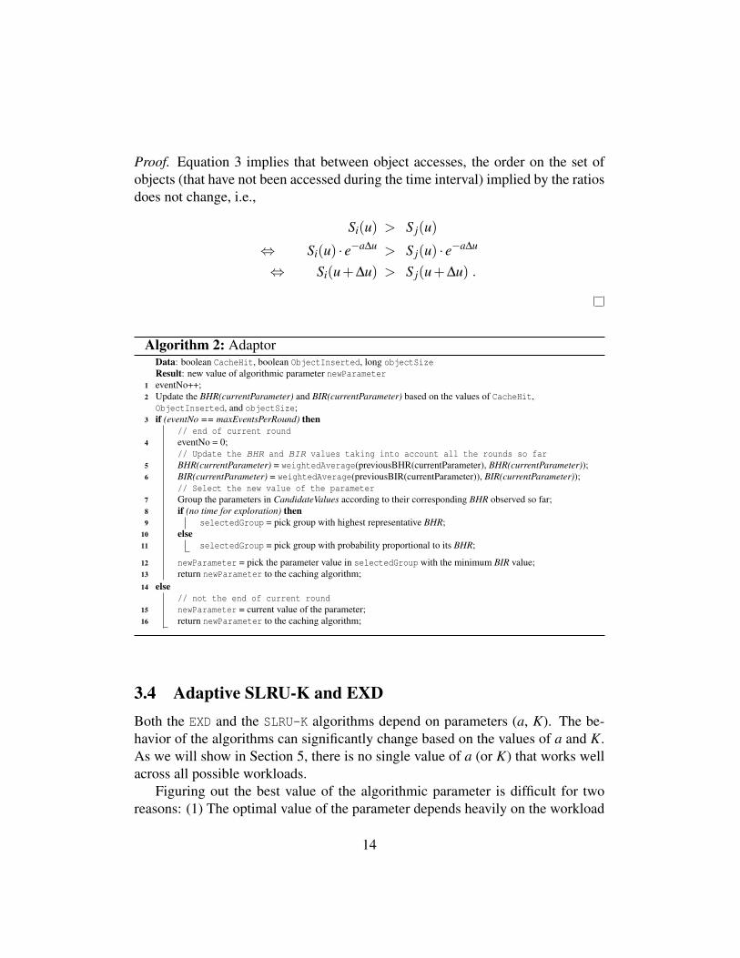
Algorithm 2: AdaptorData: boolean CacheHit, boolean ObjectInserted, long objectSizeResult: new value of algorithmic parameter newParameter

1 eventNo++;2 Update the BHR(currentParameter) and BIR(currentParameter) based on the values of CacheHit,

ObjectInserted, and objectSize;3 if (eventNo == maxEventsPerRound) then

// end of current round4 eventNo = 0;

// Update the BHR and BIR values taking into account all the rounds so far5 BHR(currentParameter) = weightedAverage(previousBHR(currentParameter), BHR(currentParameter));6 BIR(currentParameter) = weightedAverage(previousBIR(currentParameter)), BIR(currentParameter));

// Select the new value of the parameter7 Group the parameters in CandidateValues according to their corresponding BHR observed so far;8 if (no time for exploration) then9 selectedGroup = pick group with highest representative BHR;

10 else11 selectedGroup = pick group with probability proportional to its BHR;

12 newParameter = pick the parameter value in selectedGroup with the minimum BIR value;13 return newParameter to the caching algorithm;14 else

// not the end of current round15 newParameter = current value of the parameter;16 return newParameter to the caching algorithm;

3.4 Adaptive SLRU-K and EXDBoth the EXD and the SLRU-K algorithms depend on parameters (a, K). The be-havior of the algorithms can significantly change based on the values of a and K.As we will show in Section 5, there is no single value of a (or K) that works wellacross all possible workloads.

Figuring out the best value of the algorithmic parameter is difficult for tworeasons: (1) The optimal value of the parameter depends heavily on the workload

14

access pattern, and (2) The workload access pattern is not stable over time. In thissection, we present an adaptive algorithm (Adaptor) that automatically adjuststhe value of the algorithmic parameter in order to improve overall performance.

The Adaptor can be used with both the SLRU-K and the EXD methods. It oper-ates along with the caching algorithm and exchanges information with it. Each ob-ject access is treated as an event. At every event, the caching algorithm informsthe Adaptor whether the event was a cache miss or a cache hit, and whether theobject was inserted into the cache. The Adaptor uses this information to adjustthe algorithmic parameters over time.

The Adaptor takes into account two metrics when making decisions about thevalue of the algorithmic parameter. The primary metric is the byte hit ratio (BHR)which is a standard comparative performance metric used in prior work on cachingvariable-size objects [6, 29, 2, 27]. The BHR is the fraction of the requested bytesthat was served from the cache. The higher the BHR, the fewer I/O requests needto be made, and the greater the overall performance. As in previous work, ourprimary goal is to maximize the BHR.

In an external caching system, such as in HDFS cache, cache insertions com-pete for resources with the process that needs to access the data, and thereby slowdown the workload. To quantify the overhead of each algorithm with respect tocache insertions, we introduce a secondary metric, namely the byte insertion ratio(BIR). The BIR is the fraction of the requested bytes that the caching algorithmdecided to insert into the cache.

In our environment, it is desirable to maximize the BHR so that the hot set isalways cached while maintaining a low BIR if possible. Our Adaptor constantlyevaluates the behavior of the caching algorithm by measuring these metrics, andits primary goal is to maximize the BHR. From all the values of the algorithmicparameter that maximize the BHR, the Adaptor prefers the one that minimizesthe BIR, since it reduces the cost of insertions in the cache.

The pseudocode for the Adaptor is presented in Algorithm 2. The algorithmuses a set of pre-defined parameter values, namely CandidateValues. In case of theSLRU-K algorithm, the CandidateValues set contains the following values for theK parameter: 1,2,4,6,8. In the case of the EXD algorithm, the CandidateValuesset contains six a values equally-spaced in the log space with amin = 10−12 andamax = 0.3. These values cover a large range of potential parameter instantiationsthat can successfully be applied in many workload scenarios. For each potentialvalue of the algorithmic parameter i ∈ CandidateValues, the Adaptor maintainsthe observed BHR(i) and BIR(i) achieved with the value i so far.

The algorithm operates on rounds that consist of a fixed number of events.

15

After every event, the Adaptor updates the BHR and BIR values observed forthe current value of the parameter (currentParameter), based on the informationreceived from the caching algorithm (Line 2).

When the last event of the round is processed, the BHR and the BIR val-ues that correspond to the current parameter value are updated using a weightedaverage over the observed BHR and BIR values across all rounds, giving moreemphasis on the observations of the last round (Lines 3-6). The Adaptor thenre-evaluates the value of the algorithmic parameter. The re-evaluation processconsists of three steps. In the first step, the Adaptor groups the parameter valuesof the CandidateValues set, according to their observed BHR so far. Parametervalues with BHR values within a certain threshold of each other are placed in thesame group (Line 7). Each group has a representative BHR value, which is theaverage of the BHR of its members. In the next step, the Adaptor picks the groupwith the highest representative BHR (Lines 8,9). Occasionally, at this step, theAdaptor selects a group with probability proportional to the BHR of the group(Lines 10,11). This happens so that the parameter space is explored by observingthe behavior of the caching algorithm for different values of the parameter. Aftera group has been selected, the Adaptor selects a member of this group by takinginto account the BIR values that have been achieved so far by the members ofthe group. More specifically, it picks the parameter value that has resulted in thelowest BIR so far (Line 12).

After the value of the parameter has been selected, the Adaptor informs thecaching algorithm of the new value (Lines 13,16). The caching algorithm, then,updates the ratios of the objects in the History and the CacheState to reflect thenew value.

4 System ImplementationIn this section, we briefly describe the implementation of our caching algorithmsin Big SQL [5], IBM’s SQL-on-Hadoop offering, which is part of the IBM®

InfoSphere® BigInsightsTM data platform. We use the HDFS cache mechanismthat is part of the HDFS file system, and is supported by the platform.

Big SQL [5] leverages IBM’s state-of-the-art relational database technologyto execute SQL queries over HDFS data, supporting all the common Hadoop fileformats; text, sequence, Parquet and ORC files. The Big SQL coordinator com-piles and optimizes the query. The database workers read HDFS data directly andexecute relational operations.

16

A fundamental component in Big SQL is the scheduler service, which as-signs HDFS blocks to database workers for processing on a query by query basis.The scheduler identifies where the HDFS blocks are, and decides which databaseworkers to include in the query plan. The assignment is done dynamically at run-time to accommodate failures: scheduler uses the workers that are currently upand running. In case of partitioned tables, which are common in SQL-on-Hadoopenvironments, selection predicates are pushed down to the scheduler to eliminatepartitions that are not relevant for a given query. As the scheduler is aware ofwhich data objects are accessed for each query, we incorporated our caching al-gorithms in the scheduler service.

The caching algorithm operates at the level of table partitions, considering un-partitioned tables as consisting of a single partition. While each partition mayitself consist of multiple HDFS files of different sizes, the caching algorithmmaintains metadata (see Section 3) per-partition rather than per-file to minimizememory footprint. For every scan operation in a query, the Big SQL schedulerfirst eliminates unnecessary partitions, and then invokes the caching algorithm todecide which partitions to insert into the HDFS cache. The scheduler uses theappropriate HDFS APIs [13] to instruct HDFS to cache a partition. Note thatHDFS performs the actual cache insertions, not Big SQL. The Big SQL sched-uler runs a separate thread for the Adaptor, in case of adaptive algorithms. Thisthread communicates with the thread running the caching algorithm to exchangethe necessary information (see Section 3.4).

The HDFS cache [13] implements its own algorithms to decide which replicaof a given block will be cached, and in which DataNode. During query execution,the Big SQL scheduler always attempts to assign data to worker nodes optimizingfor data locality in a best effort fashion, giving priority to memory locality, andthen disk locality. More specifically the scheduler, gathers the locations of all thereplicas of a given block that will be accessed by the query, and attempts to firstassign the in-memory replicas to the workers that host them, then assigns the localon-disk replicas, and finally incorporates accesses to remote replicas.

Data on HDFS may occasionally change. For example, deletion of files, fileappends, or file additions in a table or partition can be performed without goingthrough the Big SQL interface. For this reason, the caching algorithm maintains atimestamp for each partition (table) in the cache. The timestamp is the time of thelatest modification of all the files that comprise the partition (or table). When thepartition (or table) is accessed again, the algorithm checks the latest modificationtime for this data to identify potential data changes since the last time this datawas accessed. In case there has been a change, the algorithm compares the new

17

size of the data with the size of the previous access. If the new size is smallerthan the one stored in the metadata, then one or more deletion operations havebeen performed and some files would no longer reside in the HDFS cache. Thisis because, when a cached HDFS file is deleted, HDFS automatically removesit from the HDFS cache. In this case, the caching algorithm only updates itsmetadata (latest modification time, new size of the data). In case of file appendsor additions, the partition (or table) is removed from the cache, and we try tore-insert it into the cache with its new data size.

5 Experimental EvaluationIn this section, we provide a comprehensive evaluation of our proposed algo-rithms with state-of-the-art caching policies. We begin with a simulation studywhich demonstrates how well our algorithms adapt to various data access patterns.Simulation studies, while admittedly artificial, give us fine-grained control on theworkload pattern, and allow us to reason about the comparative performance of thealgorithms without being clouded by incidental system implementation or hard-ware details (e.g., CPU efficiency, I/O and network bandwidth). For this reason,simulation studies have been extensively used to evaluate caching algorithms inprior work [23, 25, 18, 6, 20, 31, 17, 27]. We, then, back up these findings withexperimental results running IBM’s Big SQL on various workloads in a clusterenvironment in Section 5.2.

5.1 Simulation Study5.1.1 Simulator Design

To evaluate our algorithms under various scenarios, we implemented a simulationframework that generates synthetic workloads accessing data objects whose sizesare drawn from various distributions. The simulator framework is similar to theone used in [10] in the context of Map-Reduce, but is extended to accommodateobjects of different sizes.

The simulator framework consists of a data object generator and three work-load generators. The data generator creates a database D, consisting of objectswith different sizes, drawn from various distributions such as fixed (constant), uni-form, log-normal, and log-uniform distributions. The workload generators gener-ate sequences of accesses to these objects.

18

The frequency-based workload generator Wf emphasizes the frequency of ob-ject accesses. For example, in a partitioned table in a SQL-on-Hadoop system,it is likely that the last year’s partitions will be more frequently accessed thanpartitions from a decade ago. Wf generates a workload in which objects from apredefined subset, namely, the coreSet, are accessed more frequently than the re-maining objects. The Wf generator either picks an object at random, uniformly,from the coreSet (with probability p f ), or uniformly from D (with probability1− p f ).

The recency-based workload generator Wr emphasizes the recency of objectaccesses. More specifically, Wr keeps a sliding window, called the stickiness win-dow, over the sequence of object accesses. The stickiness window size determinesthe number of recently-accessed objects that are more likely to be accessed againin future requests; the larger the stickiness window size, the longer an object willpersist in the workload. The Wr generator either picks an object at random, uni-formly, from the stickiness window (with probability pr), or uniformly from D.In the latter case, the selected object will be inserted into the stickiness window,applying an LRU eviction policy if necessary.

The hybrid workload generator Wh generates a workload with both frequencyand recency characteristics. Given a probability parameter ph, to generate eachaccess, Wh invokes either Wr with probability ph or Wf with probability 1-ph. Inthis case, the hotset evolves over time based on the recent accesses, but it alsocontains some objects, which are accessed more frequently than others.

5.1.2 Evaluation

In this section, we present our results using our simulation framework. We nowpresent our experimental setting:• Data: We generated a database of size 1M, using objects whose sizes were

drawn uniformly from the range [1,1999].1 This distribution allows us to eval-uate scenarios with a wide range of data object sizes. In the interest of brevity,we omit similar results that we obtained by varying the distribution width, andchoosing other size distributions such as log-normal or log-uniform.

• Evaluation Metrics: We evaluate various caching algorithms using the byte hitratio (BHR) and the byte insertion ratio (BIR) metrics (see Section 3.4). Whencomparing algorithms, our primary goal is to maximize the BHR. Among all thealgorithms that maximize the BHR, we prefer the one that minimizes the BIR,

1The unit of data size does not affect the results.

19

30%

40%

50%

By

te H

it R

ati

o (

%)

LRU-1

LRU-2

LRU-6

SLRU-2

SLRU-6

0%

10%

20%

0% 5% 10% 15% 20% 25% 30% 35%

By

te H

it R

ati

o (

%)

Cache Size (proportional to the database size)

EXD (1E-12)

EXD (3E-1)

GDS

Adaptive EXD

Adaptive SLRU-K

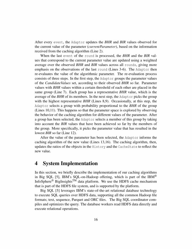
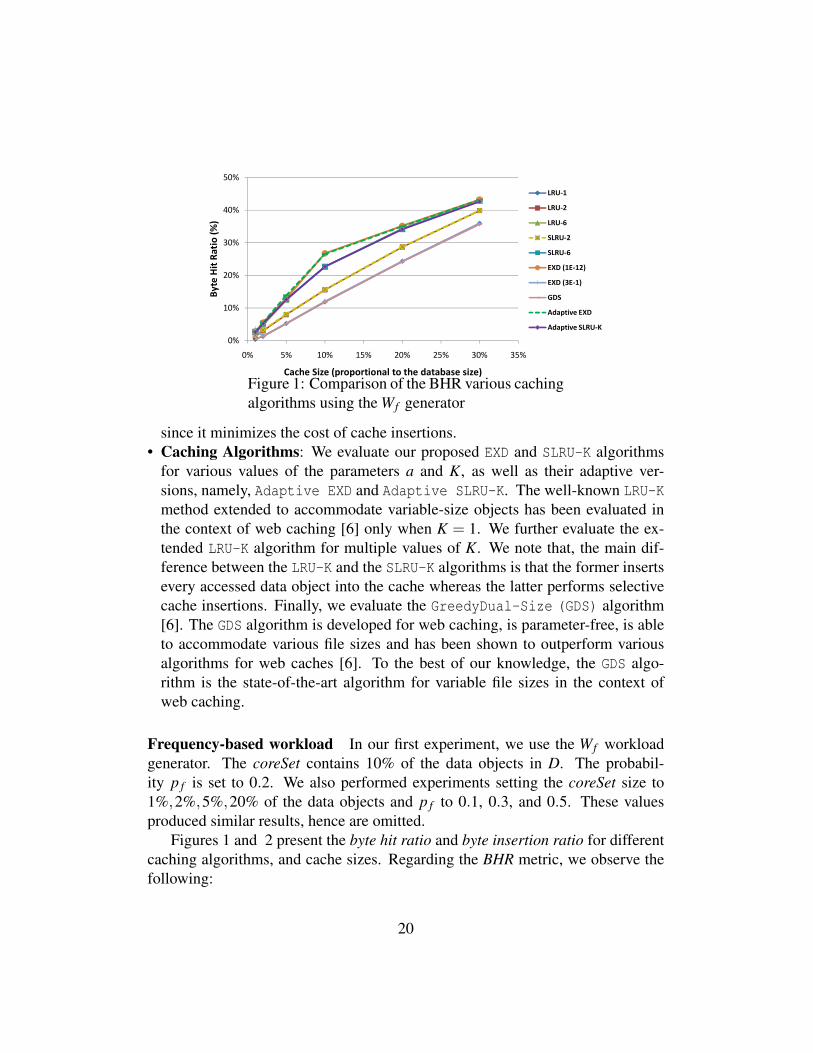
Figure 1: Comparison of the BHR various cachingalgorithms using the Wf generator

since it minimizes the cost of cache insertions.• Caching Algorithms: We evaluate our proposed EXD and SLRU-K algorithms

for various values of the parameters a and K, as well as their adaptive ver-sions, namely, Adaptive EXD and Adaptive SLRU-K. The well-known LRU-Kmethod extended to accommodate variable-size objects has been evaluated inthe context of web caching [6] only when K = 1. We further evaluate the ex-tended LRU-K algorithm for multiple values of K. We note that, the main dif-ference between the LRU-K and the SLRU-K algorithms is that the former insertsevery accessed data object into the cache whereas the latter performs selectivecache insertions. Finally, we evaluate the GreedyDual-Size (GDS) algorithm[6]. The GDS algorithm is developed for web caching, is parameter-free, is ableto accommodate various file sizes and has been shown to outperform variousalgorithms for web caches [6]. To the best of our knowledge, the GDS algo-rithm is the state-of-the-art algorithm for variable file sizes in the context ofweb caching.

Frequency-based workload In our first experiment, we use the Wf workloadgenerator. The coreSet contains 10% of the data objects in D. The probabil-ity p f is set to 0.2. We also performed experiments setting the coreSet size to1%,2%,5%,20% of the data objects and p f to 0.1, 0.3, and 0.5. These valuesproduced similar results, hence are omitted.

Figures 1 and 2 present the byte hit ratio and byte insertion ratio for differentcaching algorithms, and cache sizes. Regarding the BHR metric, we observe thefollowing:

20

50%

60%

70%

80%

90%

100%

By

te I

nse

rtio

n R

ati

o (

%)

LRU-1

LRU-2

LRU-6

SLRU-2

SLRU-6

0%

10%

20%

30%

40%

50%

0% 5% 10% 15% 20% 25% 30% 35%

By

te I

nse

rtio

n R

ati

o (

%)

Cache Size (proportional to the database size)

EXD (1E-12)

EXD (3E-1)

GDS

Adaptive EXD

Adaptive SLRU-K

Figure 2: Comparison of the BIR various cachingalgorithms using the Wf generator

1. The value of K significantly affects the behavior of both the LRU-K and theSLRU-K with greater values of K providing higher BHR. This is because thelower the value of K, the more emphasis is given by the algorithm on the re-cency than the frequency of data accesses, which is the focus of the Wf gener-ator.

2. The LRU-K and the SLRU-K algorithms have very similar BHR for the samevalue of K, since both algorithms use the same probability function, and thusidentify similar hotsets. However, the performance of the two algorithms dif-fers with respect to the BIR metric as we discuss next.

3. The performance of the EXD algorithm with respect to the BHR metric variessignificantly as the parameter a varies. More specifically, the lower the valueof a the better the BHR since a lower a gives more emphasis on the frequencyof object accesses.

4. The GDS algorithm has similar BHR values to the LRU-1 and EXD(0.3) algo-rithms, both of which give emphasis to recency.

5. Finally, the parameter-free Adaptive EXD and the Adaptive SLRU-K algo-rithms are able to identify the correct values of K and a that result in high BHRfor all cache sizes. Notice that the Adaptive EXD provides slightly better BHRvalues.

Regarding the BIR metric, we can observe the following:1. The SLRU-K algorithm has significantly lower BIR than the LRU-K algorithm

for the same value of K due to the weight heuristic that attempts to avoidunnecessary insertions whereas LRU-K performs an object insertion for everycache miss.

21

2. As the value of K decreases, the BIR of the SLRU-K metric decreases. Whenthe value of K is small, the algorithm gives more emphasis on the recency ofdata accesses, trying to maintain the most recently accessed data in the cache,thus incurring a large number of cache insertions. Obviously, this behavior isnot desirable for workloads generated by the Wf generator.

3. The performance of the EXD algorithm with respect to the BIR metric varieswith the parameter a. More specifically, the lower the value of a, e.g., 10−12,the better the BIR since a lower a gives more emphasis on the frequency ofobject accesses, and less on the recency of accesses.

4. The GDS algorithm has similar BIR values to the LRU-1 and EXD(0.3) algo-rithms, both of which give emphasis to recency.

5. The adaptive Adaptive EXD and the Adaptive SLRU-K algorithms are ableto identify the correct values of K and a that result in low BIR for all cachesizes. Notice that the Adaptive EXD can provide better BIR values than theAdaptive SLRU-K.

6. Another observation is that the trends for the BIR metric are not the same acrossdifferent algorithms. Some algorithms, like LRU-K have a very high BIR atsmall cache sizes, which decreases as the cache becomes larger. This is becausethe larger the cache size, the more objects fit in the cache and thus cache in-sertions are avoided. However, other algorithms such as EXD and SLRU-K havevery low BIR for small cache sizes. The reason is that the weight heuristicthat these algorithms use, identifies that it is not worth to keep replacing objectsin the cache when the hotset does not fit in the cache, but it is more beneficialto maintain a few popular objects in the cache. This policy results in slightlyhigher BHR than LRU-K for small cache sizes, and much lower BIR.Overall, we observe that the Adaptive EXD and the Adaptive SLRU-K algo-

rithms learn the correct values of the parameter, and thus produce high BHR, andlow BIR for all cache sizes.

Recency-based workload In the next experiment, we use the Wr workload gen-erator and set pr to 0.2 . The stickiness window contains 10% of the data objectsin D. Other values produced similar results, and hence are omitted.

Figures 3 and 4 present the BHR and the BIR values for various cachingalgorithms and cache sizes. In this case, the algorithms that value recency morethan frequency in their caching decisions (such as LRU-1, EXD(0.3), GDS) exhibitthe best BHR performance. Notice that these algorithms also have the highest BIRvalues. This is not surprising since insertions are necessary in order to keep up

22

30%

40%

50%

By

te H

it R

ati

o (

%)

LRU-1

LRU-2

LRU-6

SLRU-2

SLRU-6

0%

10%

20%

0% 5% 10% 15% 20% 25% 30% 35%

By

te H

it R

ati

o (

%)

Cache Size (proportional to the database size)

EXD (1E-12)

EXD (3E-1)

GDS

Adaptive EXD

Adaptive SLRU-K

Figure 3: Comparison of the BHR various cachingalgorithms using the Wr generator

50%

60%

70%

80%

90%

100%

By

te I

nse

rtio

n R

ati

o (

%)

LRU-1

LRU-2

LRU-6

SLRU-2

SLRU-6

0%

10%

20%

30%

40%

50%

0% 5% 10% 15% 20% 25% 30% 35%

By

te I

nse

rtio

n R

ati

o (

%)

Cache Size (proportional to the database size)

EXD (1E-12)

EXD (3E-1)

GDS

Adaptive EXD

Adaptive SLRU-K

Figure 4: Comparison of the BIR various cachingalgorithms using the Wr generator

with hotsets that are based on the recency of data accesses. In other words, inorder to observe high BHR values on workloads with hotsets that mainly includethe most recent data accesses, an algorithm must not avoid insertions; otherwise,accesses on the hot data will result in cache misses. Note however, that a high BIRvalue does not necessarily mean that the “correct” data is actually cached. Forexample, the LRU-2, LRU-6 algorithms have lower BHR than LRU-1, althoughthey have similar or higher BIR value. This is because they give less emphasis onthe recency of data accesses.

Another observation is that the Adaptive SLRU-K and the Adaptive EXD al-gorithms are able to achieve very good BHR values. The BIR values of thesealgorithms are very low for small cache sizes, and then significantly increase for

23

15%

20%

25%

30%

By

te H

it R

ati

o (

%)

LRU-1

LRU-2

LRU-6

SLRU-2

SLRU-6

0%

5%

10%

15%

0 0.1 0.2 0.3 0.4 0.5 0.6 0.7 0.8 0.9 1

By

te H

it R

ati

o (

%)

Probability of using Wr (ph)

EXD (1E-12)

EXD (3E-1)

GDS

Adaptive EXD

Adaptive SLRU-K

Figure 5: Comparison of the BHR various cachingalgorithms using the Wh generator

60%

80%

100%

By

te I

nse

rtio

n R

ati

o (

%)

LRU-1

LRU-2

LRU-6

SLRU-2

SLRU-6

0%

20%

40%

0 0.1 0.2 0.3 0.4 0.5 0.6 0.7 0.8 0.9 1

By

te I

nse

rtio

n R

ati

o (

%)

Probability of using Wr (ph)

EXD (1E-12)

EXD (3E-1)

GDS

Adaptive EXD

Adaptive SLRU-K

Figure 6: Comparison of the BIR various cachingalgorithms using the Wh generator

cache sizes greater than 5% of the database size. The reason for this behavior isthat when the hotset is much larger than the available cache space, the adaptivealgorithms make the decision to cache a small set of objects and do not replacethem frequently. In this way, they are able to get a higher BHR than algorithms likeEXD(0.3), which generally behaves very well for recency-based workloads. Asthe cache size increases, and more hot data can be accommodated in the cache, theadaptive algorithms do not avoid insertions in order to always cache the evolvinghotset. In summary, the adaptive Adaptive EXD and the Adaptive SLRU-K al-gorithms produce high BHR for all cache sizes by making correct cache insertiondecisions.

24

Hybrid workload In our final experiment, we use the Wh workload generator.In this example, the coreSet as well as the stickiness window contain 10% of thedata objects in D, and their corresponding probabilities p f and pr are both set to0.2. Initially, the coreSet and the stickiness window contain different objects. Weset the cache size to 10% of the database size (other cache sizes produced similarresults), and vary the probability of using the Wr generator (ph).

Figures 5 and 6 show the BHR and the BIR values for various values of ph.When ph = 0, only the Wf generator is invoked and thus the algorithms that valuefrequency such as LRU-6, SLRU-6 and EXD(10−12) produce the best BHR val-ues. As the value of ph increases, and thus the Wr generator also gets invoked,the performance of these algorithms with respect to the BHR becomes worseand algorithms such as GDS, EXD(0.3) start becoming better. When ph = 1, thefrequency-based algorithms have the worst behavior, whereas the recency-basedalgorithms produce the best BHR. An interesting point is that the Adaptive EXDand Adaptive SLRU-K methods are able to adjust the values of K and a so thatthey can produce good BHR results irrespective of the value of ph. None of theother algorithms exhibit this adaptive behavior, as they are only optimized for spe-cial workload characteristics. Similarly, the adaptive methods adjust the numberof insertions they perform in order to get the best result. When ph is high, theadaptive methods perform insertions in order to keep up with the recency char-acteristics of the hotset. Finally, we again observe that the adaptive SLRU-K andEXD algorithms have lower BIR values than the non-adaptive algorithms when thatdoes not negatively impact the BHR values.

5.1.3 Summary

Our simulations use a variety of workloads, varying the extent to which the ac-cess pattern of objects is affected by frequency and recency of past accesses tothem. Overall, we observed that the basic SLRU-K and EXD algorithms for differ-ent parameters achieve high BHR and low BIR for different workloads, but noneof them individually performs well on all of them. However, the adaptive algo-rithms, especially the Adaptive EXD algorithm, achieve the best balance betweenBHR and BIR, effectively producing the lowest BIR without negatively affectingthe BHR. Finally, none of the traditional algorithms can consistently outperformour Adaptive EXD algorithm across different workload patterns.

25

0.79

0.70

0.66

0.64

0.63

EXD(1E-12)

SLRU-2

LRU-2

EXD(3E-1)

LRU-1

0.85

0.80

0.79

0.0 0.2 0.4 0.6 0.8 1.0

Prophetic (OPT)

Adaptive EXD

Adaptive SLRU-K

EXD(1E-12)

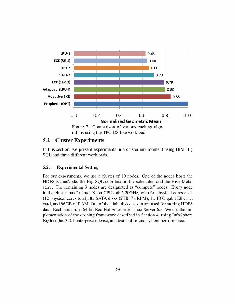
Normalized Geometric MeanFigure 7: Comparison of various caching algo-rithms using the TPC-DS like workload

5.2 Cluster ExperimentsIn this section, we present experiments in a cluster environment using IBM BigSQL and three different workloads.

5.2.1 Experimental Setting

For our experiments, we use a cluster of 10 nodes. One of the nodes hosts theHDFS NameNode, the Big SQL coordinator, the scheduler, and the Hive Meta-store. The remaining 9 nodes are designated as “compute” nodes. Every nodein the cluster has 2x Intel Xeon CPUs @ 2.20GHz, with 6x physical cores each(12 physical cores total), 8x SATA disks (2TB, 7k RPM), 1x 10 Gigabit Ethernetcard, and 96GB of RAM. Out of the eight disks, seven are used for storing HDFSdata. Each node runs 64-bit Red Hat Enterprise Linux Server 6.5. We use the im-plementation of the caching framework described in Section 4, using InfoSphereBigInsights 3.0.1 enterprise release, and test end-to-end system performance.

26

5.2.2 TPC-DS Like Workload

In this section, we present cluster experiments using a workload inspired by theTPC-DS benchmark2. This workload is published by Impala developers3, andhas previously been used to compare the performance of various SQL-on-Hadoopsystems (e.g., [28], [11]). The workload consists of 20 queries that include multi-way joins, aggregations, and nested sub-queries. The fact table is partitioned,whereas the small dimension tables are not partitioned. We use a 3TB TPC-DSdatabase, and a 300GB HDFS cache.

We compare the different caching algorithms with a theoretically optimal ref-erence algorithm, which we call the Prophetic prefetcher. Before runningeach query, this algorithm uses prior knowledge of the entire workload trace toprefetch as much of the data accessed by the next query as fits in the cache. As aresult, all but 2 of the 20 queries ran entirely in memory. Further, the evaluation ofProphetic prefetcher only measures the execution time of the queries, ignor-ing the time to prefetch the data into memory4. For each algorithm, we performedthe experiment 3 times using a warm HDFS cache, and report the average over the3 runs.

Figure 7 shows the geometric mean of the running times of various caching al-gorithms normalized to the running time of the offline Prophetic Prefetcher.As shown, the adaptive algorithms achieve the best performance. The Propheticprefetcher was only about 15% faster than the Adaptive EXD algorithm eventhough it had a priori knowledge of the entire workload. The remaining algo-rithms were not as efficient as the adaptive algorithms. For example, the LRU-1algorithm achieved 63% of the Prophetic Prefetcher’s performance.

The workload’s total elapsed time was 2713 seconds when using the LRU-1method and 2556 seconds with the LRU-2 method. The total elapsed time using theAdaptive EXD algorithm was 1711 seconds. This is an important difference, es-pecially if we consider that the best possible performance that can be achieved byan offline algorithm is 1544 seconds (Prophetic Prefetcher). Figure 8 showsthe runtime of each query normalized to the query runtime using the PropheticPrefetcher. Ideally, a caching algorithm should produce query runtimes closeto the ones produced by the Prophetic Prefetcher. As shown in the figure, theadaptive algorithms generally resulted in query runtimes close to those observed

2http://www.tpc.org/tpcds/3https://github.com/cloudera/impala-tpcds-kit4Recall that reading the data into the cache incurs additional cost that needs to be paid by

external caches

27

Figure 8: Normalized Query Runtime for theTPC-DS like workload

when the Prophetic Prefetcher was used. The LRU-1 algorithm, on the otherhand, did not perform as well as the adaptive methods. When comparing the bestperforming online algorithm (Adaptive EXD) with the LRU-1 algorithm, we ob-serve that all but one of the queries experienced speedups ranging from 1.03X to2.3X , and the geometric mean of the speedups was 1.34X .

We also performed experiments with other values of the parameter K. The be-havior was similar to the LRU-2 and SLRU-2 methods and these results are omittedin the interest of space. Our results show that: (1) the adaptive algorithms grace-fully adapt over time to produce the best performance results, and (2) the perfor-mance achieved is close to the one achieved by a hypothetical offline algorithmthat prefetches the data needed by each query.

5.2.3 Hotset experiment

The goal of this experiment is to show which algorithms are able to correctlyidentify the workload’s hotset, and how performance is affected. Our evaluationcompares the various caching algorithms with the HotSet Prefetcher, an algo-rithm that has a priori knowledge of the entire workload, prefetches and cachesthe hotset of partitions.

The TPC-DS like queries that we used in the previous experiment access awide range of data that keeps evolving over time making it difficult to identifythe workload’s hotset, and use the HotSet Prefetcher to upper-bound the per-formance. 5 For this reason, we created a workload that operates on the 1TBstore sales TPC-DS fact table, and has a clear hotset. In this way, we can

5This is the reason we use the the per-query Prophetic Prefetcher to upper-bound perfor-mance of the TPC-DS like workload.

28

evaluate which caching algorithms are able to identify this hotset.Our workload consists of 50 queries that contain selections, projections and

aggregations. We have observed that corporate users of Big SQL and Hadooptend to frequently access their recent data, and more rarely their older/historicaldata, while creating summaries for reports. Thus, the workload’s hotset consistsof the 250 most recently created partitions. Each query in our workload accesses asubset of the table’s partitions. A partition is accessed either from the most recent250 partitions uniformly at random with probability 0.5 (hotset), or uniformlyfrom the set of the remaining 1550 older partitions (coldset). The total size ofthe 250 most frequently accessed partitions is approximately 170GB. We used a170GB HDFS cache so that the hotset fits entirely in the cache.

Figure 9 shows the performance of the algorithms that we tested. The chartplots the geometric mean of the running times of the algorithms normalized tothe running time using the HotSet Prefetcher. As shown in the figure, theEXD(10−12) algorithm provided almost the same performance as the HotSet Prefetcher.This is expected as this workload is essentially the best use-case for this algorithm,which gives emphasis on the frequency of the data accesses as presented in oursimulation study. However, other values of a produce different (worse) perfor-mance (e.g, EXD(0.3)). The parameter-free, adaptive methods were able to achieveabout 95% of the performance of the HotSet Prefetcher.

The total elapsed time of the workload with the Adaptive EXD method wasabout 615 seconds, while the total elapsed time with the offline HotSet Prefetcherwas 549 seconds. Note that the adaptive algorithms occasionally re-evaluate theparameter space, and thus, pay some exploration cost. Nevertheless, they are ableto perform very well under various workload patterns.

Another interesting point is that some algorithms like LRU-1 and EXD(0.3) re-sulted in higher total elapsed time for this workload (934 seconds and 885 secondsrespectively) than a system that does not use the HDFS cache at all (837 seconds).The reason is that these algorithms perform multiple cache insertions that com-pete for resources with the query engine, essentially slowing down the workload.Setting an algorithmic parameter incorrectly can result in unexpected system be-havior. When comparing the Adaptive EXD algorithm with the LRU-1 algorithm,we observe that all but seven of the individual queries experienced speedups rang-ing from 1.08X to 6.02X , and the geometric mean of the speedups was 1.44X .This result shows that not all caching algorithms are suitable for external caches,and highlights the need for parameter-free adaptive algorithms.

29

0.94

0.83

0.80

0.58

0.56

Adaptive EXD

SLRU-2

LRU-2

EXD(3E-1)

LRU-1

0.99

0.95

0.94

0.0 0.2 0.4 0.6 0.8 1.0

HotSet

EXD (1E-12)

Adaptive SLRU-K

Adaptive EXD

Normalized Geometric Mean

Figure 9: Comparison of various caching algo-rithms using the synthetic workload

5.2.4 Concurrent Workload

In this experiment, we evaluate our algorithms using a complex workload with adiverse mix of concurrent batch and interactive queries. Our goal is to investi-gate how the performance of interactive workloads that have low response timerequirements gets affected by long running analytics workloads, such as batchqueries used for reporting, running concurrently for various caching algorithms.In particular, we run batch analytics queries (the TPC-DS like workload describedin Section 5.2.2) concurrently with parallel streams of interactive queries. Theinteractive queries are continuously executed using three parallel streams until theTPC-DS like workload finishes. We, then, evaluate how the average responsetime of the interactive queries gets affected by the batch queries and how the totalelapsed time of the TPC-DS like workload varies with the caching method.

The interactive queries are aggregations over a single partition of a large, 1T Btable. The table is a copy of the TPC-DS fact table used in the previous experi-ments (Section 5.2.3). We created a separate table for the interactive queries inorder to force the batch and interactive queries to access different data sets, andthus compete more aggressively for the cache space. We used the same accesspattern for the partitions of the table as in the previous experiment. More specif-ically, the interactive queries access a partition either from the most recent 250partitions uniformly at random with probability 0.5, or uniformly from the set ofthe 1550 older partitions. Our total database size is 4T B and our HDFS cache size

30

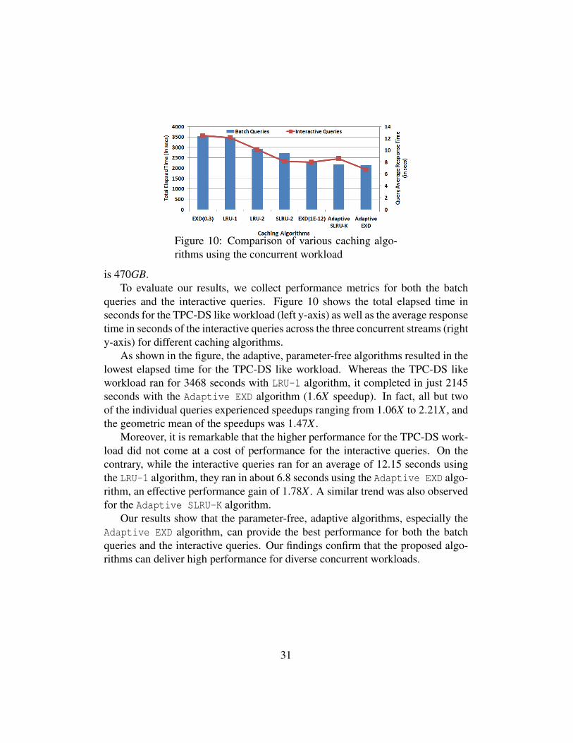
Figure 10: Comparison of various caching algo-rithms using the concurrent workload

is 470GB.To evaluate our results, we collect performance metrics for both the batch

queries and the interactive queries. Figure 10 shows the total elapsed time inseconds for the TPC-DS like workload (left y-axis) as well as the average responsetime in seconds of the interactive queries across the three concurrent streams (righty-axis) for different caching algorithms.

As shown in the figure, the adaptive, parameter-free algorithms resulted in thelowest elapsed time for the TPC-DS like workload. Whereas the TPC-DS likeworkload ran for 3468 seconds with LRU-1 algorithm, it completed in just 2145seconds with the Adaptive EXD algorithm (1.6X speedup). In fact, all but twoof the individual queries experienced speedups ranging from 1.06X to 2.21X , andthe geometric mean of the speedups was 1.47X .

Moreover, it is remarkable that the higher performance for the TPC-DS work-load did not come at a cost of performance for the interactive queries. On thecontrary, while the interactive queries ran for an average of 12.15 seconds usingthe LRU-1 algorithm, they ran in about 6.8 seconds using the Adaptive EXD algo-rithm, an effective performance gain of 1.78X . A similar trend was also observedfor the Adaptive SLRU-K algorithm.

Our results show that the parameter-free, adaptive algorithms, especially theAdaptive EXD algorithm, can provide the best performance for both the batchqueries and the interactive queries. Our findings confirm that the proposed algo-rithms can deliver high performance for diverse concurrent workloads.

31

6 Related WorkThere is a lot of work in cache replacement policies developed in various con-texts. For brevity, we point the reader to [23, 6] for a more comprehensive surveyof the existing literature. Instead, we highlight the most closely related work toplace our current work in the proper context. In the context of relational databasesand storage systems, there is extensive work on page replacement policies suchas the LRU-K [25], DBMIN [8], ARC [23], LIRS [17], LRFU [20], MQ [31] and2Q [18] policies. There is also recent work on SLA-aware buffer pool algorithmsfor multi-tenant settings [24]. Unlike our proposed algorithms, these policies op-erate on fixed size pages since they mainly target traditional buffer pool settings.Moreover, these policies assume that every accessed page has to be inserted intothe buffer pool, thus selective cache insertions lie beyond their remit. We alsonote that our algorithms focus on caching raw data, unlike approaches like se-mantic caching [9].

Many caching policies have been developed for web caches that operate onvariable size objects. The most well-known algorithms in the space are the SIZE [2],LRU-Threshold [1], Log(Size) + LRU [1], Hyper-G [2], Lowest-Latency-First [29],Greedy-Dual-Size [6], Pitkow/Recker [2], Hybrid [29], PSS [3] and Lowest Rel-ative Value (LRV) [27]. The work in [6] has extensively compared various webcaching algorithms, and has shown that the GDS algorithm outperforms them. Inthis paper, we presented experiments that compare GDS with our proposed meth-ods, and have shown that our adaptive algorithms outperform GDS.

Self-tuning and self-managing database systems have been studied in variouscontexts [7, 22]. In the context of caching, the ARC method [23] adapts its behav-ior based on the data access pattern. Unlike our algorithms, ARC operates onlyon fixed size objects and its adaptive design strongly depends on this assumption.

Exponential functions have been used before to model different types of be-havior. For example, the work in [4] uses a power law with an exponential cuttoffto model consumer behavior in various setttings. Our proposed Adaptive EXDalgorithm makes use of a parameterized exponential function to predict object re-accesses but adapts the function based on the workload access pattern. To the bestof our knowledge, this is the first time that a caching algorithm makes use of anadaptive exponential function.

In the context of Hadoop systems, Cloudera [15] and Hortonworks [13], twomajor Hadoop distribution vendors allow the users to manually pin HDFS files,partitions or tables in the HDFS cache in order to speedup their workloads. TheImpala [19] developers claim that the usage of HDFS cache can provide a 3X

32

speedup on SQL-on-Hadoop workloads [15]. In the Spark ecosystem [30], SparkRDDs can be cached in Tachyon [21], a distributed in-memory file system. Tothe best of our knowledge, these systems do not use automatic algorithms thatidentify the hotset but rather rely on the user to manually cache the data.

7 ConclusionsIn this work we propose online, adaptive algorithms for external caches in thecontext of Big Data systems. We experimentally show, through simulations andcluster experiments, that our methods are able to adjust to various workload pat-terns, and outperform a variety of existing static algorithms. Our experimentalresults show that it is essential to use an adaptive algorithm that can automaticallyadjust its behavior based on the workload characteristics. Because it is almost im-possible to know the global system workload a priori, to identify the hotset overtime, to pick the correct algorithm, and its corresponding parameter value (e.g.,K, a).

References[1] M. Abrams et al. Caching Proxies: Limitations and Potentials. Technical report,

1995.

[2] M. Abrams et al. Removal Policies in Network Caches for World-Wide Web Docu-ments. SIGCOMM Comput. Commun. Rev., 26(4), 1996.

[3] C. Aggarwal, J. L. Wolf, and P. S. Yu. Caching on the World Wide Web. IEEETrans. on Knowl. and Data Eng., 11(1), 1999.

[4] A. Anderson, R. Kumar, A. Tomkins, and S. Vassilvitskii. The dynamics of repeatconsumption. WWW ’14, 2014.

[5] Big SQL 3.0: SQL-on-Hadoop without compromise. http://www-01.ibm.com/common/ssi/cgi-bin/ssialias?infotype=SA&subtype=WH&htmlfid=SWW14019USEN#loaded.

[6] P. Cao and S. Irani. Cost-Aware WWW Proxy Caching Algorithms. In USENIX,1997.

[7] S. Chaudhuri and V. Narasayya. Self-Tuning Database Systems: A Decade ofProgress. In VLDB, 2007.

33

[8] H.-T. Chou and D. J. DeWitt. An Evaluation of Buffer Management Strategies forRelational Database Systems. In VLDB, 1985.

[9] S. Dar et al. Semantic data caching and replacement. VLDB, 1996.

[10] M. Y. Eltabakh et al. Eagle-eyed Elephant: Split-oriented Indexing in Hadoop. InEDBT, 2013.

[11] A. Floratou, U. F. Minhas, and F. Ozcan. SQL-on-Hadoop: Full Circle Back toShared-nothing Database Architectures. PVLDB, 7(12), 2014.

[12] Hadoop 2.0. http://hadoop.apache.org/docs/current/hadoop-yarn/hadoop-yarn-site/YARN.html.

[13] Hortonworks: Centralized Cache Management in HDFS. http://docs.hortonworks.com/HDPDocuments/HDP2/HDP-2.1.1/bk_system-admin-guide/content/ch_hdfs_caching.html.

[14] O. H. Ibarra and C. E. Kim. Fast Approximation Algorithms for the Knapsack andSum of Subset Problems. J. ACM, 22(4), 1975.

[15] HDFS Read Caching. http://blog.cloudera.com/blog/2014/08/new-in-cdh-5-1-hdfs-read-caching/.

[16] K. Iwama and S. Taketomi. Removable Online Knapsack Problems. 2380:293–305,2002.

[17] S. Jiang and X. Zhang. LIRS: An Efficient Low Inter-reference Recency Set Re-placement Policy to Improve Buffer Cache Performance. In ACM SIGMETRICS,2002.

[18] T. Johnson and D. Shasha. 2Q: A Low Overhead High Performance Buffer Man-agement Replacement Algorithm. In VLDB, 1994.

[19] M. Kornacker et al. Impala: A Modern, Open-Source SQL Engine for Hadoop. InCIDR, 2015.

[20] D. Lee et al. LRFU: A Spectrum of Policies That Subsumes the Least Recently Usedand Least Frequently Used Policies. IEEE Trans. Comput., 50(12), 2001.

[21] H. Li, A. Ghodsi, M. Zaharia, S. Shenker, and I. Stoica. Tachyon: Reliable, MemorySpeed Storage for Cluster Computing Frameworks. In SOCC, 2014.

[22] S. Lightstone et al. Control Theory: a Foundational Technique for Self ManagingDatabases. In ICDE Workshops, 2007.

34

[23] N. Megiddo and D. S. Modha. ARC: A Self-Tuning, Low Overhead ReplacementCache. In FAST, 2003.

[24] V. Narasayya et al. Sharing Buffer Pool Memory in Multi-tenant RelationalDatabase-as-a-service. PVLDB, 8(7), 2015.

[25] E. J. O’Neil, P. E. O’Neil, and G. Weikum. The LRU-K Page Replacement Algo-rithm for Database Disk Buffering. In ACM SIGMOD, 1993.

[26] K. Ren, Y. Kwon, M. Balazinska, and B. Howe. Hadoop 's Adolescence: A Com-parative Workload Analysis from Three Research Clusters, 2012.

[27] L. Rizzo and L. Vicisano. Replacement Policies for a Proxy Cache. IEEE/ACMTrans. Netw., 8(2), 2000.

[28] TPC-DS like Workload on Impala. http://blog.cloudera.com/blog/2014/09/new-benchmarks-for-sql-on-hadoop-impala-1-4-widens-the-performance-gap/.

[29] R. P. Wooster and M. Abrams. Proxy Caching That Estimates Page Load Delays.Computer Networks, 29(8-13), 1997.

[30] M. Zaharia et al. Resilient Distributed Datasets: A Fault-tolerant Abstraction forIn-memory Cluster Computing. NSDI, 2012.

[31] Y. Zhou, J. Philbin, and K. Li. The Multi-Queue Replacement Algorithm for SecondLevel Buffer Caches. In USENIX, 2001.

35