RC24755 (W0903-015) March 4, 2009Computer Science

IBM Research Report

Extended Compressed Sensing: Filtering Inspired Methods for Sparse Signal Recovery

and Their Nonlinear Variants

Avishy CarmiDepartment of EngineeringUniversity of Cambridge

United Kingdom

Pini GurfilTechnion - Israel Institute of Technology

Haifa 32000Israel

Dimitri Kanevsky, Bhuvana RamabhadranIBM Research Division

Thomas J. Watson Research CenterP.O. Box 218

Yorktown Heights, NY 10598

Research DivisionAlmaden - Austin - Beijing - Cambridge - Haifa - India - T. J. Watson - Tokyo - Zurich

1

Extended Compressed Sensing:Filtering Inspired Methods for SparseSignal Recovery and Their Nonlinear

VariantsAvishy Carmi,Member, IEEE, Pini Gurfil, Member, IEEE, Dimitri

Kanevsky and Bhuvana Ramabhadran

Abstract

New methods are presented for sparse signal recovery from a sequence of noisy observa-tions. The sparse recovery problem, which is NP-hard in general, is addressed by resortingto convex and non-convex relaxations. The body of algorithms in this work extends andconsolidate the recently introduced Kalman filtering (KF)-based compressed sensing methods.These simple methods, which are briefly reviewed here, rely on a pseudo-measurement trickfor incorporating the norm relaxations following from CS theory. The extension of the methodsto the nonlinear case is discussed and the notion of local CS is introduced. The essential idea isthat CS can be applied for recovering sufficiently small and sparse state perturbations therebyimproving nonlinear estimation in cases where the sensing function maps the state onto a lower-dimensional space. Other two methods are considered in thiswork. The extended Baum-Welch(EBW), a popular algorithm for discriminative training of speech models, is amended herefor recovery of normalized sparse signals. This method naturally handles nonlinearities andtherefore has a prominent advantage over the nonlinear extensions of the KF-based algorithmswhich rely on validity of linearization. The last method derived in this work is based ona Markov chain Monte Carlo (MCMC) mechanism. This method roughly divides the sparserecovery problem into two parts. Thus, the MCMC is used for optimizing the support ofthe signal while an auxiliary estimation algorithm yields the value of elements. An extensivenumerical study is provided in which the methods are compared and analyzed. As part of this,the KF-based algorithm is applied to lossy speech compression.

I. INTRODUCTION

Recent studies have shown that sparse signals can be recovered accurately using less observa-tions than what is considered necessary by the Nyquist/Shannon sampling principle; the emergent

Manuscript received ; revised .A. Carmi is with the Signal Processing Group, Department of Engineering, University of Cambridge, UK.P. Gurfil is with the Faculty of Aerospace Engineering, Technion – Israel Institute of Technology, Haifa 32000,

IsraelD. Kanevsky and B. Ramabhadran are with IBM T. J. Watson Research Center, Yorktown, NY 10598, USA

2

theory that brought this insight into being is known as compressed sensing (CS) [1]–[3]. Theessence of the new theory builds upon a new data acquisition formalism, in which compressionplays a fundamental role. From a filtering standpoint, one can think about a procedure in whichsignal recovery and compression are carried out simultaneously, thereby reducing the amountof required observations. Sparse, and more generally, compressible signals arise naturally inmany fields of science and engineering. A typical example is the reconstruction of images fromunder-sampled Fourier data as encountered in radiology, biomedical imaging and astronomy [4],[5]. Other applications consider model-reduction methodsto enforce sparseness for preventingover-fitting and for reducing computational complexity andstorage capacities. The reader isreferred to the seminal work reported in [3] and [2] for an extensive overview of the CS theory.

The recovery of sparse signals is in general NP-hard [1], [6]. State of the art methods foraddressing this optimization problem commonly utilize convex relaxations, non-convex localoptimization and greedy search mechanisms. Convex relaxations are used in various methodssuch as LASSO [7], the Dantzig selector [8], basis pursuit and basis pursuit de-noising [9], andleast angle regression [10]. Non-convex optimization approaches include Bayesian methodologiessuch as the relevance vector machine otherwise known as sparse Bayesian learning [11] aswell as stochastic search algorithms which are mainly basedon Markov chain Monte Carlotechniques [12]–[15]. Notable greedy search algorithms are the matching pursuit (MP) [16], theorthogonal MP [17], and the orthogonal least squares [18].

CS theory has drawn much attention to the convex relaxation methods. It has been shownthat the convexl1 relaxation yields an exact solution to the recovery problemprovided twoconditions are met: 1) the signal is sufficiently sparse, and2) the sensing matrix obeys theso-called restricted isometry property (RIP) at a certain level. Another complementary resultensures high accuracy when dealing with noisy observations. Further elaboration of this resultfacilitated its probabilistic version which is concluded by the known statement of recovery‘with overwhelming probability’. To put it informally, it is highly probable for the convexl1relaxation to yield an exact solution provided the involvedquantities, the sparseness degrees,and the sensing matrix dimensionsm× n maintain relation of the type

s = O(m/ log(n/m))

Influential as it may be, the theory of CS at its current stage deals with a parameter estimationproblem in which the observations are merely a linear projection onto a lower dimensional space

y = Hx+ ζ, H ∈ Rm×n

In this work we are taking the underlying model two steps further, though not entirely from thetheoretical standpoint.Step 1:The numerical recipes derived in this work are aimed at solvingthe discrete-time linear filtering problem where the noisy observation model assumes the aboveformulation. Here the time-varying signal is described viathe state dynamics

xk+1 = Axk + wk, k = 0, 1, 2, . . .

It can be easily verified that if for instanceA = I (i.e., xk is a random walk) then full recon-struction of the statexk using the above measurement model is strictly infeasible. Nevertheless,

3

if the underlying signal is sparse in some basis then by introducing the knownl1 relaxation,accurate recovery is possible.

Step 2: Another extension which is of much interest involves the nonlinear counterpart ofthe above observation model

y = h(x) + ζ, h : Rn → R

m

In this work we present the notion of local RIP of the sensing functionh which in turn facilitatesthe implementation of local CS. The idea here is that CS can beused to recover small and sparseperturbations∆x from a nominal statex∗. The l1 relaxation then takes the form

min ‖ ∆x ‖1 s.t. ‖ y − h(x∗ + ∆x) ‖2< ε

which is approximately equivalent to

min ‖ ∆x ‖1 s.t. ‖ y − [∂h/∂x]x∗ ∆x ‖2< ε

where y = y − h(x∗). The approximate linear form above facilitates the application of theconventional CS where the estimation performance depends on the local RIP coefficient whichis a property of the Jacobian[∂h/∂x]. This idea is further shown to improve the estimationperformance of the extended Kalman filter when applied to thenonlinear observation model.

Algorithms: In broad, three types of algorithms are derived for solving the above mentionedproblems. These account for 1) CS-embedded Kalman filter (CSKF) that was initially introducedin [19]–[21] and reviewed here for completeness, 2) Sparse Extended Baum-Welch (EBW), and3) Stochastic subset search (S3). We remark here that our work is not the first attempt to combineCS and KF. The Kalman filtering approach presented in [22] relies on an auxiliary optimizationprocedure (e. g., the Dantzig selector of [8]) and is capableof coping with time varying sparsesignals. The method suggested inhere is based on a pseudo-measurement (PM) formulation ofthe underlying constrained optimization problem. Compared to the algorithm in [22], this methodcan be straightforwardly implemented in a stand-alone manner, as it is exclusively based on thewell-known KF formulation.

1) The CSKF has three variants each of which is based on a different relaxation. The CSKF-1uses thel1 norm relaxation while the CSKF-p utilizes a quasi-norm formulation with lp,p ∈ (0, 1). The third variant is based on a uniquel0 norm approximation.

2) The sparse EBW method is based on a widely used algorithm inspeech recognition. Thismethod essentially maximizes a lower bound of a general objective function defined overa probability domain. The method is shown to naturally handle sparse directional vectors(i.e., ‖ x ‖1= 1) and is guaranteed to converge.

3) The stochastic subset search is a Monte Carlo type method that uses both a simulatedannealing core and a point process representations for finding the signal support. Theestimated support is then fed to a conventional KF algorithm. This method is inspired bya Markov chain Monte Carlo scheme used for filtering of randomfinite sets.

Nonlinear Extensions:

4

1) A nonlinear variant of the CSKF is the CS-EKF. This algorithm utilizes the notion oflocal CS for recovering a sparse signal based on the aforementioned nonlinear observationmodel.

2) The sparse EBW naturally handles the nonlinear observation model and is essentiallyshown to outperform the CS-EKF in the normalized case (i.e.,for ‖ x ‖1= 1).

This paper is organized as follows. The next section mathematically formulates the sparse re-covery problem. Section III provides a brief overview of thevarious CSKF algorithms. Local CSalong with the nonlinear CS-EKF implementation are discussed in Section IV. The sparse EBWoptimization method is introduced in Section V. Section describes the stochastic subset searchmethod. Section VII provides the results of an extensive numerical study that had been carriedout for assessing and comparing the various estimation methods. The last part of this sectiondemonstrate the application of the CSKF to lossy speech compression. Finally, conclusions areoffered in the last section.

II. L INEAR ESTIMATION OF SPARSESIGNALS

Consider anRn-valued random discrete-time process{xk}∞k=1 that is sparse in some knownorthonormal sparsity basisψ ∈ R

n×n, that is

zk = ψTxk, #{supp(zk)} < n (1)

wheresupp(zk) and# denote the support ofzk and the cardinality of a set, respectively. Assumethat zk evolves according to

zk+1 = Azk + wk, z0 ∼ N (µ0, P0) (2)

whereA ∈ Rn×n and{wk}∞k=1 is a zero-mean white Gaussian sequence with covarianceQk ≥ 0.

Note that (2) does not necessarily imply a change in the support of the signal. For example,A can be a block-diagonal matrix decomposed ofAd andAn corresponding to the statisticallyindependent elementszd /∈ supp(zk) andzn ∈ supp(zk) where the respective noise covariancesub-matrices satisfyQd = 0 andQn ≥ 0. The processxk is measured by theRm-valued randomprocess

yk = Hxk + ζk = H ′zk + ζk (3)

where{ζk}∞k=1 is a zero-mean white Gaussian sequence with covarianceRk > 0, andH :=H ′ψT ∈ R

m×n.Letting yk := [y1, . . . , yk], our problem is defined as follows. We are interested in finding a

yk-measurable estimator,xk, that is optimal in some sense. Often, the sought after estimator isthe one that minimize the mean square error (MSE)E

[

‖ xk − xk ‖22

]

. It is well-known that ifthe linear system (2), (3) is observable, i.e.,

O :=[

HT (HA)T · · · (HAn−1)T]T

rank(O) = n (4)

then the solution to this problem can be obtained using Kalman filtering. On the other hand, ifthe system is unobservable, then the regular KF algorithm isuseless; if, for instance,A = In×n,

5

then it may seem hopeless to reconstructxk from an under-determined system in whichm < nand rank(H) < n. Surprisingly, this problem may be circumvented by taking into account thefact thatzk is sparse.

A. The Combinatorial Problem and Compressed Sensing

Refs. [1], [6] have shown that in the deterministic case (i. e., whenz is a parameter vector),one can accurately recoverz (and therefore alsox, i.e., x = ψz) by solving the optimizationproblem

min ‖ z ‖0 s.t.k∑

i=1

‖ yi −H ′z ‖22≤ ε (5)

for a sufficiently smallε, where‖ v ‖p=(

∑nj=1 v

pj

)1/pis the lp-norm ofv, and the zero-norm,

‖ v ‖0, is defined as1 ‖ v ‖0 := # {supp(v)}.Following a similar rationale, in the stochastic case the sought-after optimal estimator satis-

fies [2]min ‖ zk ‖0 s.t.Ezk|yk

[

‖ zk − zk ‖22

]

≤ ε (6)

Unfortunately, the above optimization problems are NP-hard and cannot be solved efficiently.Recently, it has been shown that if the sensing matrixH ′ obeys a so-calledrestricted isometryproperty(RIP) while z is sparse enough possibly with [2]

s = O(m/ log(n/m)) (7)

wheres = #{supp(z)}, then the solution of the combinatorial problem (5) can almost alwaysbe obtained by solving the constrained convex optimization[1], [2]

min ‖ z ‖1 s.t.k∑

i=1

‖ yi −H ′z ‖22≤ ε (8)

This is a fundamental result in the new emerging theory of compressed sensing (CS) [1], [2].The main idea is that the convexl1 minimization problem can be efficiently solved using amyriad of existing methods, such as LASSO [7], the Dantzig selector [8], Basis pursuit andBasis pursuit de-noising [9], and least angle regression [10], to mention only a few.

III. K ALMAN FILTERING COMPRESSEDSENSING

It was only a matter of time until the Kalman filter, the work-horse of linear estimation theory,would be employed for compressed sensing. The popularity ofthe KF algorithm is owing toits ease of implementation and its modest computational demands (with respect to some otherknown estimation methods) as well as to its well-known statistical properties, such as being

1For 0 ≤ p < 1, ‖ v ‖p is not a norm; the common terminology iszero normfor p = 0 and quasi-normfor0 < p < 1.

6

the best minimum MSE (MMSE) linear estimator around (which coincides with the optimalestimator in the MMSE sense for linear Gaussian systems) [23].

The first successful attempt for Kalman filtering-based compressed sensing was presentedin [22] where the traditional KF algorithm was endowed with the Dantzig selector of [8].This approach divides the sparse recovery problem into two interlaced subproblems: 1) supportextraction, and 2) reduced order recovery. This separationroughly specifies a two phase algorithmin which some CS method (in this case the Dantzig selector) identifies the subset of elementsin the support of the signal while the ordinary KF is applied for the reduced order systemcorresponding to the obtained subset. This approach, whichis termedinterlaced CSapproachin this work, proved itself to be very successful as was demonstrated in [22].

A rather straightforward approach for solving the sparse filtering problem using KF wasrecently introduced in [19]–[21]. The suggested methods inboth these works are based on a well-known trick for incorporating nonlinear equality constraints into the traditional KF formulation.Compared with the interlaced CS approach which involves an external optimization procedure,these methods are fairly simple to implement and requires nomajor modifications in the originalKF structure. The emphasize here is on simplicity which makes these methods viable andappealing for many filtering applications. For completeness we revisit here the main conceptsfrom [19]–[21].

1) Pseudo-Measurement Trick:For the system described by (2) and (3) the classical KFprovides an estimatezk that is a solution to the unconstrainedl2 minimization problem

minzk

Ezk|yk

[

‖ zk − zk ‖22

]

Inspired by the CS approach while retaining the KF objectivefunction, we replace (6) by theconstrained optimization

minzk

Ezk|yk

[

‖ zk − zk ‖22

]

s.t. ‖ zk ‖1≤ ε′ (9)

This procedure is based on the following proposition which is given here without a proof.Proposition 1 ( [21]): Let y and Y be an observation random variable and its realization,

respectively. Let alsox and x be a random variable and its associatedy-measurable estimator,respectively. Giveny = Y , the optimization problems

minxEx|y

[

‖ x− x ‖22

]

s. t. ‖x‖1 ≤ ε1 (10)

minx

‖x‖1 s. t. Ex|y

[

‖x− x‖22

]

≤ ε2 (11)

with ε1, ε2 > 0, are equivalent.The constrained optimization problem (9) can be solved in the framework of Kalman filtering

using the pseudo-measurement (PM) technique [24], [25]. The idea is fairly simple: the inequalityconstraint‖ zk ‖1≤ ε′ is incorporated into the filtering process using a fictitiousmeasurement0 =‖ zk ‖1 −ε′, whereε′ serves as a measurement noise. This PM can be rewritten as

0 = Hzk − ε′, H := [sign(zk(1)), . . . , sign(zk(n))] (12)

7

where sign(zk(i)) denotes the sign function of theith element ofzk (i.e., sign(zk(i)) = 1 ifzk(i) > 0 and equals 0 otherwise) . In this setting, the covarianceRε of ε′ is regarded as atuning parameter, which can be determined based on simulation runs. A single iteration of theCS-embedded KF is detailed in Algorithm 12.

Algorithm 1 CSKF-1 [21]

1: Predictionzk+1|k = Azk|k (13a)

Pk+1|k = APk|kAT +Qk (13b)

2: Measurement UpdateKk = Pk+1|kH

′T(

H ′Pk+1|kH′T +Rk

)−1(14a)

zk+1|k+1 = zk+1|k +Kk

(

yk −H ′zk+1|k

)

(14b)

Pk+1|k+1 = (I −KkH′)Pk+1|k (14c)

3: CS Pseudo Measurement:Let P 1 = Pk+1|k+1 and z1 = zk+1|k+1.4: for τ = 1, 2, . . . , Nτ − 1 iterationsdo5:

Hτ = [sign(zτ (1)), . . . , sign(zτ (n))] (15a)

Kτ = P τ HTτ

(

HτPτ HT

τ +Rε

)−1(15b)

zτ+1 = (I −Kτ Hτ )zτ (15c)

P τ+1 = (I −Kτ Hτ )P τ (15d)

6: end for7: SetPk+1|k+1 = PNτ and zk+1|k+1 = zNτ .

2) Quasi-Norm Constrained Variants:A different approach for approximately solving thecombinatorial problem in (6) is based on replacing‖ · ‖0 by a quasi-norm‖ · ‖p with 0 < p < 1.This approach has already been shown to yield better accuracy compared to thel1 norm [6].

Following the previous section methodology, the PM technique is used here to incorporatethe quasi-norm inequality constraint‖ zk ‖p≤ ε′ by producing the fictitious measurement

0 =‖ zk ‖p −ε′

whereε′ serves as a zero-mean Gaussian measurement noise with covarianceRε. In practice,this PM is linearized around some nominal statez∗k to yield

0 =

(

n∑

i=1

|z∗k(i)|p)1/p

+ H∆zk − ε′ + O(‖ ∆zk ‖22) (16)

2Notice that this is an unusual implementation of the KF as thematrix Hτ is state dependent.

8

wherezk(i) denotes theith element ofzk, the perturbation∆zk := zk − z∗k, and

H(i) =

{

(∑n

i=1 |z∗k(i)|p)1/p−1 [z∗k(i)]p−1 , if z∗k(i) > 0

− (∑n

i=1 |z∗k(i)|p)1/p−1 [−z∗k(i)]p−1 , if z∗k(i) ≤ 0, i = 1, . . . , n (17)

is the ith element ofH. This formulation facilitates the implementation of an extended KF(EKF) stage for incorporating the PM. Following this, the nominal statez∗k is set as the updatedestimate at timek.

A single iteration of the resulting KF algorithm with the linearized PM stage is similar toAlgorithm 1 with a slight modification in the PM implementation as described in Algorithm 2.

Algorithm 2 PM Stage of The CSKF-p [21]

1: Pseudo Measurement:Let P 1 = Pk+1|k+1 and z1 = zk+1|k+1.2: for τ = 1, 2, . . . , Nτ − 1 iterationsdo3: ComputeHτ using (17) withz∗k = zτ .

Kτ = P τ HTτ

(

HτPτ HT

τ +Rε

)−1(18a)

zτ+1 = zτ −Kτ ‖ zτ ‖p (18b)

P τ+1 = (I −Kτ Hτ )P τ (18c)

4: end for5: SetPk+1|k+1 = PNτ and zk+1|k+1 = zNτ .

3) Approximatel0 Norm: The l0 norm can alternatively be approximated by

n−n∑

i=1

exp (−α|zk(i)|) (19)

for large enoughα > 0. The corresponding PM stage in that case consists of the samesteps(18) where (18b) is replaced by

zτ+1 = zτ +Kτ

[

n−n∑

i=1

exp (−α|zτ (i)|)]

(20)

(i.e., the PM isn =∑n

i=1 exp (−α|zk(i)|) + ε′) whereH is given by

H(i) =

{

−α exp (−αz∗k(i)) , if z∗k(i) > 0α exp (αz∗k(i)) , if z∗k(i) ≤ 0

, i = 1, . . . , n (21)

IV. EXTENDED COMPRESSEDSENSING

At its current stage the theory of CS deals with the recovery of signals that are linearlyprojected onto a lower dimension observation space. One could naturally wonder whether asimilar set of rules apply in the case of arbitrary smooth mappings. The formulation would then

9

be the following. Given a sufficiently smooth mappingh : Rn → R

m, m < n and somes-sparsevectorz ∈ R

n that obey the observational relationyi = h(z) + ζ, i = 1, . . . , k, then to whatextent and under what conditions can we recoverz from y using thel1 relaxation suggested byCS, i.e., by solving

min ‖ z ‖1 s.t.k∑

i=1

‖ yi − h(z) ‖22≤ ε (22)

It should be mention that such a nonlinear observation modelwas recently addressed in [26],though from a greedy standpoint, i.e., by generalizing the orthogonal matching pursuit algorithm.In this work we are not going to fully answer the above stated question but rather demonstratehow CS can be applied for recovering sufficiently small sparse perturbations from a givennominal state.

One of the fundamental results in CS is that accurate and possibly exact recovery of sparsesignals is feasible depending on the RIP level of the sensingmatrix [2]. The RIP is closelyrelated to the the Johnson-Lindenstrauss (JL) lemma which is stated about general Lipschitzlow-distortion embeddings [27].

Lemma 1 (JL):Given someδ ∈ (0, 1), a setZ of l points in Rn and a numberm0 =

O(ln(l)/δ2), there is a Lipschitz functionh : Rn → R

m wherem > m0 such that

(1 − δ) ‖ z − z∗ ‖2≤‖ h(z) − h(z∗) ‖2≤ (1 + δ) ‖ z − z∗ ‖2 (23)

for all z, z∗ ∈ Z.Now, consider a case wherez = z∗ + ∆z with sufficiently small‖ ∆z ‖2, then by taking the

first-order Taylor expansion ofh(z) aroundz∗ it can be easily recognized that the JL lemmareduces to approximately the RIP of the Jacobian[∂h/∂z] computed locally atz∗, that is

(1 − δ) ‖ ∆z ‖2≤‖ [∂h/∂z]z∗ ∆z + o(

‖ ∆z ‖22

)

‖2≤ (1 + δ) ‖ ∆z ‖2 (24)

In that sense the Lipschitz function that satisfies the JL relation (23) locally obeys the RIP atz∗ for the perturbation vector∆z. The property (24) of the sensing functionh(z) is termedLocal RIP in this work. Similarly to the linear case, the level of the local RIP ofh(z) at z∗ isdetermined according to the maximal sparseness degrees of the perturbation∆z for which (24)holds. Obviously, when considering the recovery of a sufficiently small and sparse∆z, CS canbe applied where the Jacobian[∂h/∂z]z∗ takes the role of the traditional sensing matrix. Thel1relaxation would then have the form

min ‖ ∆z ‖1 s.t.k∑

i=1

‖ yi − h(z∗ + ∆z) ‖22≤ ε (25)

where the accuracy of recovery would be related to the local RIP constantδs of the sensingfunction h(z).

10

A. Local CS and Nonlinear Estimation: The CS-Embedded EKF

Maybe the most interesting implication that follows from the local CS idea is that thel1relaxation can improve conventional nonlinear estimationmethods that are based on linearizationsuch as the EKF. In such methods the linearization around some predetermined nominal point,which is usually taken as the best up to date estimate, facilitates the application of a linearestimator (e.g., the KF) for reconstructing the perturbed state. The sensing matrix in this case ismerely the Jacobian of the sensing function locally computed at the nominal point whereas thestate transition matrix is taken as the Jacobian of the time propagation function. Now, considera case in which the sensing functionh(z) maps the state onto a lower-dimensional space, thenfollowing the preceding argument it is expected that local CS will allow better recovery ofsufficiently sparse perturbation∆z provided thath(z) obeys the local RIP at a proper level.

In this work we have implemented the local CS idea by amendingthe CSKF algorithms ofSection III for nonlinear estimation. The slight modification consists of replacing the ordinaryKF recursion with an EKF one while retaining the desired PM stage (i.e., corresponding to thel1, the lp or the approximatel0 norms).

V. SPARSEOPTIMIZATION : THE EXTENDED BAUM -WELCH

Extended Baum-Welch (EBW) is a popular optimization technique in speech recognition tooptimize discriminative objective functions [28]. As the name suggests, EBW is an extension ofthe BW algorithm. The Baum-Welch (BW) algorithm is an expectation-maximization algorithmthat computes maximum likelihood estimates and posterior mode estimates for the parameters(transition and emission probabilities) of a Hidden MarkovModel, when given only emissionsas training data [29]. The BW algorithm can be used to optimize non-negative polynomials overprobability domains. More precisely it can be used to solve the following problem:

maxzQ(z) s.t.z ∈ P = {zij ≥ 0,

mi∑

j=1

zij = 1} (26)

andQ is a polynomial with non-negative coefficients andP is a discrete probability domain.This is an iterative procedure that uses the Jensen inequality to reduce the optimization foreach recursive step to optimization of an auxiliary function overP . The auxiliary function isestimated at each step and is a weighted sum oflog zij . In practical tasks that require maximum-likelihood estimates of HMM with large number of parametersthe BW method became popularbecause it is easy to implement, it usually requires a small number of iterations to get tonear optimum and each iteration requires number of computations that is proportional to anumber of parameters. The BW algorithm was not applicable directly to discriminative estimationproblems for HMM that required optimization of (26) whereQ was a polynomial with somenegative coefficients since the Jensen inequality could notbe applied there. Twenty years agothe following simple trick was found how to extend BW methodsto polynomials that containnegative coefficients [28]. It was observed that an optimization problem of maximzingQ doesnot change if ones adds toQ a polynomialW (z) = D(

∑

ij zij + 1)m that is a constant in the

11

probability domainP . In other wordsQ(z) +W (z) = Q(z) +D × L whereL = (∑

ij zij +1)m is a constant inP and arg maxz Q(z) = arg maxz{Q(z) + W (z)} = arg maxz{Q(z) +D × L}. Now if one takesm a degree of the polynomialQ and sufficiently largeD then allcoefficients of the polynomialQ(z) + W (z) have non-negative coefficients and therefore theJensen inequality and as a consequence the BW procedure is applicable to it. The extension ofBW to polynomials that contain negative coefficients immediately allows the extention of BWto rational functions over probability domains. Then via a suitable approximation process BWhas also been extended to discriminative functions defined over sets of Gaussian distributionsrather than discrete probabilities. EBW has become a popular method in discriminative speechrecognition tasks in the last decade because of its ease of implementation and convergenceproperties.

In this Section we show EBW recursion can be naturally applied to maximizing a differentiablefunction over a domain consisting of parameters whose q-norms equal 1. It was explained inprevious sections that 1-norm constraints lead to compressive sensing conditions. Therefore wecall EBW methods for optimizing functions over 1-norm constraints as sparse optimization.

The following theorem [30] is needed to extend EBW methods tosparse constraints.Theorem 1:Let F (z) be a function that is defined overP = {zij ≥ 0,

∑

j zij =∑j=mi

j=1 zij =

1}. Let F be differentiable atz ∈ P . Let cij = zij∂

∂zijF (z), and let z = {zij} 6= z = {zij}

wherezij =

cij + zijD∑

i cij +D(27)

Then F (z) > F (z) for sufficiently large positiveD and F (z) < F (z) for sufficiently smallnegativeD.Remark: This theorem was proved in [28] for rational functions. IfF (z) is a polynomial withnon-negative coefficients thenF (z) > F (z) for D = 0 and EBW coincides with BW. This isa special case of the fact that the ML estimation of HMM parameters via EBW coincides withthe BW.

For improved reading the proof of Theorem 1 is deferred to theAppendix.

EBW Over Fractional Norms

Let Q(y) be a differentiable function ofy = {yi} ∈ Rn, i = 1, ...n. Let us consider the

following problem:max

yQ(y) s.t. ‖ y ‖q≤ β (28)

We solve this problem by transforming (28) into a problem over a probability domain forwhich EBW update rules (27) exist. Let us consider thel1 norm, that is by settingyi = x

1/qi ,

F ({xi}) = Q({yi}) andε = βq. The problem (28) then becomes

maxx

F (x) s.t. ‖ x ‖1≤ ε (29)

Now, using the dummy variablex0 ≥ 0 the above problem is rewritten as

maxx

F (x) s.t. ‖ x ‖1 +x0 = ε (30)

12

Further lettingvi = xi/ε, i = 0, ...n, andF (x) = F ({εvi}) = G(v) we may write

maxvG(v) s.t. ‖ v ‖1= 1 (31)

Recognizing that‖ v ‖1=

∑

i

σ(vi)vi (32)

andG(v) = G({σ(vi)σ(vi)vi}) = G(σ(vi)zi) = G(z) (33)

whereσ(vi) = sign(vi), andz = {zi} = {σ(vi)vi} allows writing an equivalent problem to (29)which takes the form

maxzG(z) s.t.

∑

zi = 1, zi ≥ 0 (34)

Problems of the type (34) have an EBW based solutions that canbe obtained by iterating (27).The detailed EBW recursion for solving (29) is given in Algorithm 3.

Algorithm 3 Sparse Directional EBW

1: Set intial conditionsx0 s.t. ‖ x0 ‖1= 12: for t = 0, 1, . . . , Nt iterationsdo3: Setzt

i = σ(xti)x

ti

4: Gt(zt) = F ({σ(xt

i)σ(xti)x

ti}) = F (σ(xt

i)zti)

5: Compute coefficents

cj = cj(zt) =

∂Gt(zt)

∂ztj

6: AdaptD according to some rule, e.g.,D∗ = argmaxD Gt({zt+1

i (D)})7: Update estimate

zt+1

i = zt+1

i (D) =(ci +D)zt

i∑

j cjztj +D

8: end for

A. TuningD

Note that the sign ofzt+1i in Algorithm 3 depends on how large isD. Namely, it is positive

for sufficiently largeD and is negative ifci + D < 0. In practice, instead of computation ofD∗ = arg maxD Gt{zt+1

i (D)} one can use various approximate schemes. As a general ruleDshould increase significantly when a local maximum of an objective function is approached. Oneway to achieve this is to chooseD that is inversely proportional to some degree of a gradient toan objective function at a point that is being updated duringan iterative optimization process.Various gradient steepness metrics that could be used for tuning D for EBW update rules forGaussian parameters are described in [31]. Several popularstrategies for tuningD in speechrecognition tasks are introduced in [32].

13

VI. STOCHASTIC SUBSET SEARCH

In recent years, Monte Carlo (MC) methods and in particular Markov chain MC (MCMC) havebeen successfully implemented for vast high-dimensional optimization and filtering applications.Their popularity is a direct consequence of their flexibility, their problem solving capabilities andthe ever increasing processing power of todays computers. Being a simulation based approach,MCMC generally imposes no restrictions on the characteristics of the problem being solved. Inaddition, smart strategies that have been developed over the past years improved the efficiencyof these methods when dealing with multi-modality and varying dimensionality [33]. The readeris referred to [34]–[37] for extensive overview and applications of MCMC.

In this section we derive a MCMC-based sparse recovery algorithm. The MCMC approachinhere is inspired by the particles algorithm used in [38] for multi-target tracking. However, inthis work the MCMC particles mechanism is used for optimization rather than for filtering. Theformal derivation proceeds as follows.

A. Random Set Representations

We exploit the following formulation which is used for representing random finite sets.Consider aRn-valued indicators random vectore of which each element may take either values0 or 1. Havingei = 1 implies that theith element is active. The indicators vector is associatedwith a vectorz = [z1, . . . , zn]T . Both these quantities represent a random setS, that is

S = {zi | ei = 1, i = 1, . . . , n} (35)

In the context of our sparse recovery problem the vectore represents the unknown support of thesignal and is essentially optimized using a MCMC mechanism whereas the corresponding valuesin S are obtained using a traditional KF. In that sense, this technique follows theinterlaced CSconcept discussed in Section III.

B. MCMC Particles

Suppose that at every time stepk we haveN candidates (particles){ek(j), zk(j)}Nj=1. Each

particle represents a set of dimension∑

i eik(j) that correspond to a subset of the sensing matrix

H ′. Let us denoteH(j) the subset corresponding to thejth particle, that is,H(j) = {H ′i |

eik(j) = 1, i = 1, . . . , n} whereH ′i denotes theith column ofH ′. We define for each particle

a scoring function of the form

L(S(j)) = exp

{

−1

2(1 − γk)

(

yk −H(j)S(j))T

Vk(j)−1(

yk −H(j)S(j))

}

(36)

where thejth set S(j) is taken as the output of an auxiliary estimator that was applied forprocessingyk with an initial stateS(j) and a sensing matrixH(j). As it would become clearin the ensuing, the time-dependent scaling parametersγk ∈ [0, 1] andVk(j) ∈ R

m×m affect the

14

sampling efficiency of the method. In this work we have used a KF for obtainingS(j) whereVk is set accordingly as the innovations covariance, that is

Vk = H(j)PkH(j)T +Rk (37)

wherePk is the corresponding KF covariance. At this point we use the Metropolis-Hastings(MH) algorithm for producing an improved particles population. Thus, every new candidateS(j)′, j = 1, . . . , N is accepted with probability ofL(S(j)′)/L whereL denotes the scoringfunction of the previously accepted one. The obtained population serves as the initial set ofparticles at the next time step{ek+1(j), zk+1(j)}N

j=1. The estimated signal{e∗k, z∗k} is thentaken as the one having the maximal acceptance rate.

Similarly to the cooling schedule in simulated annealing, here, the ‘tempering’ parameterγk

is used for regulating the algorithm’s convergence rate. The ability of the algorithm to overcomelocal maxima traps greatly depends on a good choice of the cooling scheme. Following a thumb-rule from MH theory, a fairly good tempering schedule allowsaccepting between 20% to 40%of the purposed candidates [37].

C. Birth/Death Moves

A good exploration of the search space is maintained by incorporating birth/death type moves.In this work the indicatorseik, i = 1, . . . , n are assumed to evolve according to a Markov chainwith the transition kernel

p(eik | eik−1 = j) =

{

aj, if eik = j1 − aj , otherwise

(38)

whereaj denotes the probability of staying in statej ∈ [0, 1].

VII. N UMERICAL STUDY

In this section we demonstrate the performance of the derived algorithms as well as someadditional concepts that were introduced in previous sections. A major part here is devoted tothe comparison of the various algorithms in different cases. Thus, the CSKF variants (i.e., thel1, the lp and the approximatel0 norms) are compared with the sparse EBW implementationas well as with the S3 method. We demonstrate the performance of the CSKF algorithms bothin the static and dynamic cases. We then proceed on with the nonlinear implementations, theCS-EKF endowed with the various norms that are compared withthe sparse EBW method. Inaddition, example is given that exemplifies the implementation of the S3 method for finding theRIP coefficient of an arbitrary matrix. The last part of this section demonstrates the applicationof the CSKF for lossy speech compression.

15

A. Static Case

The following example is partially based on the one in [19]–[21]. Here the signalz ∈ R256

is assumed to be a sparse parameter vector (i.e.,A = I256×256, Qk = 0). The signal supportconsists of total of 10 elementsz(i) 6= 0 of which both the index and value are uniformlysampled overi ∼ Ui[1, 256]

3 and z(i) ∼ U [−10, 10], respectively. The sensitivity matrixH ′

consists of72 rows in which the elements are sampled from a Gaussian distributionN (0, 1/72).The columns ofH ′ are normalized following the example in [22] (this matrix has been shownto satisfy the RIP at a sufficient level, see [2], [22]). The observation noise covariance is set asRk = 0.0012I72×72.

1) Algorithms Settings:The tuning covarianceRε of the CSKF-p was set as200002 and2002 for p = 0.5 andp = 1, respectively. The alternativel0 approximation (19) is implementedusingα = 1 andRε = 1002 (these values were chosen based on tuning runs for achievingidealperformance in terms of accuracy).

The sparse EBW was implemented using the following objective function

G(z) = p(y | z) ∝k∏

i=1

exp

{

−1

2

(

yi −H ′z)TR−1

i

(

yi −H ′z)

}

(39)

using not more than 10 iterations per time step. The estimation procedure was performed in asequential fashion by taking the best estimate of the preceding time step as the initial state forthe next one.

The S3 algorithm used a total of 1000 particles. The cooling parameter was set asγ0 = 1−10−7

and was rapidly reduced at increments of10−6. The birth/death moves probability was set asaj = 0.9 for j = 0, 1. These settings maintained an average of 30% acceptance rate of the MH.

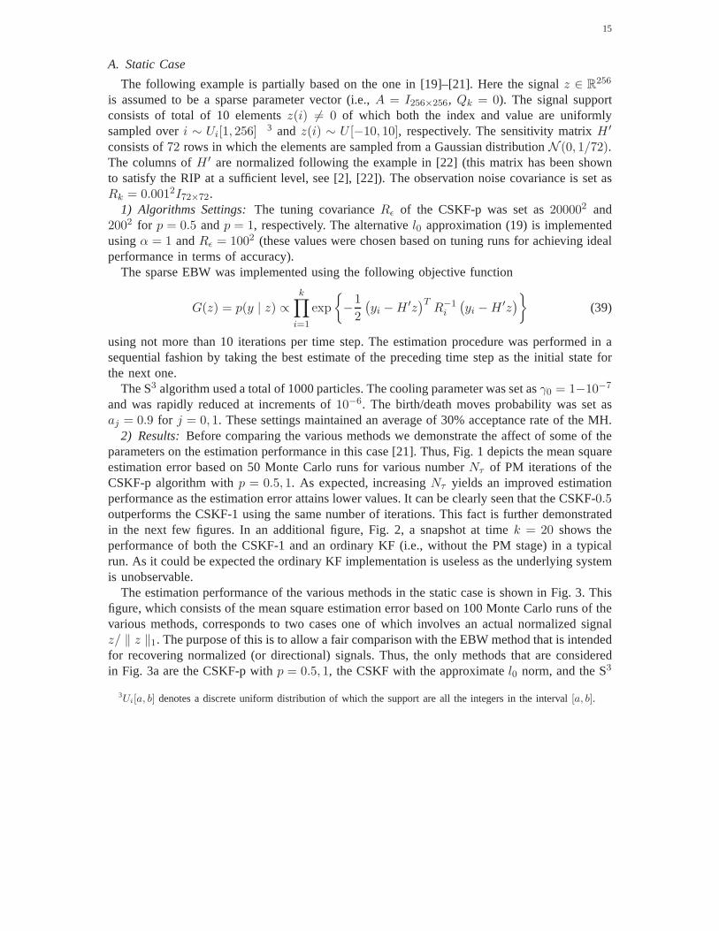
2) Results:Before comparing the various methods we demonstrate the affect of some of theparameters on the estimation performance in this case [21].Thus, Fig. 1 depicts the mean squareestimation error based on 50 Monte Carlo runs for various numberNτ of PM iterations of theCSKF-p algorithm withp = 0.5, 1. As expected, increasingNτ yields an improved estimationperformance as the estimation error attains lower values. It can be clearly seen that the CSKF-0.5outperforms the CSKF-1 using the same number of iterations.This fact is further demonstratedin the next few figures. In an additional figure, Fig. 2, a snapshot at timek = 20 shows theperformance of both the CSKF-1 and an ordinary KF (i.e., without the PM stage) in a typicalrun. As it could be expected the ordinary KF implementation is useless as the underlying systemis unobservable.

The estimation performance of the various methods in the static case is shown in Fig. 3. Thisfigure, which consists of the mean square estimation error based on 100 Monte Carlo runs of thevarious methods, corresponds to two cases one of which involves an actual normalized signalz/ ‖ z ‖1. The purpose of this is to allow a fair comparison with the EBWmethod that is intendedfor recovering normalized (or directional) signals. Thus,the only methods that are consideredin Fig. 3a are the CSKF-p withp = 0.5, 1, the CSKF with the approximatel0 norm, and the S3

3Ui[a, b] denotes a discrete uniform distribution of which the support are all the integers in the interval[a, b].

16

2 4 6 8 100

0.5

1

1.5

2

Number of Observations

MS

E

(a) CSKF-1

2 4 6 8 100

0.5

1

1.5

2

Number of Observations

MS

E

(b) CSKF-0.5

Fig. 1: Mean square estimation error based on 50 runs of the CSKF-1 (a) and of the CSKF-0.5(b) for various numbers of PM iterations. The lines, top to bottom, correspond to 50, 100, and200 pseudo-measurement iterations. Static case. [19]–[21]

method. It can be clearly seen that the best estimation accuracy is attained while using either thequasi-normlp with p = 0.5 or the S3 algorithm. Both these algorithm attain estimation accuracyat the level of the observation noise (i.e.,10−3). The alternativel0 approximation is slightlyless accurate but tends to converge faster. The CSKF-1 Algorithm exhibits inferior estimationaccuracy with respect to the other methods. The estimation performance of an ordinary KF thatis aware of the signal support is shown to attain errors of approximately 0.9 × 10−3, slightlybetter than the CSKF-0.5 and the S3. Proceeding to Fig. 3b, the EBW exhibits inferior estimationperformance compared to the CSKF-1 (and respectively with all other variants of the CSKF). TheEBW version that allows the recovery of negative componentsis shown to perform worser thanits non-negative counterpart mainly due to some runs at which the algorithm did not converge.

The 1σ bounds corresponding toz(1) − z(1) as computed by the various filters in a singlerun are shown in Fig. 4. It can be seen that these bounds reflectthe accuracy when using thedifferent norms in the CS stage. We have already seen that thebest estimation performance wasachieved by the CSKF-0.5 and correspondingly its 1σ bounds are the tightest.

B. Dynamic Case

The various CSKF algorithms are applied to filtering of sparse random-walk processes in[19]–[21]. The reader is, therefore, referred to these works for additional details and insights.

Here we have excluded both the EBW and S3 methods for the following reasons. In itsformulation presented inhere, the EBW is not suitable for the recovery of random processes. Itshould be noted that this issue is a part of the authors ongoing research. The implementation of

17

0 50 100 150 200 250−10

−5

0

5

10

Index

(a) CSKF-1

0 50 100 150 200 250−10

−5

0

5

10

Index

(b) Regular KF

Fig. 2: A snapshot atk = 20 in a typical run of the CSKF-1 (a) usingNτ = 200 PM iterationsand of an ordinary KF (b). Showing the elements of the actual (squares) and estimated (lines)signals. Static case.

the S3 algorithm for this case is trivial and does not reflect the performance of the subset searchmechanism.

C. Nonlinear Extensions

This part of the numerical study demonstrates the idea of extended CS (or local CS) ofSection IV and its application to nonlinear estimation. We consider a recovery problem consistingof the following nonlinear observation model

yi = h(z) + ζi, h(z) = H ′[

diag(z)11

2 1 + az(j)1]

(40)

where1 denotes a vector of which all entries are 1’s,a is some constant, andj is an arbitrarynumber between 1 andn. The Jacobian matrix of the sensing functionh(z) is given by

∂h

∂z= 1

1

2H ′diag(z)

1

2 + aH ′diag(ej) (41)

whereej ∈ Rn has itsjth entry equals one while all others are zero. Similarly to the previous

examples, the random matrixH ′ ∈ R72×256 has its entries independently sampled from a zero-

mean normal distribution with variance1/72. The vectorz has 10 non-zero elements of whichthe locations are uniformly sampled over the integers in theinterval [1, 256]. The values of theelements in the support ofz are uniformly sampled between[0.5, 1.5]. All other algorithm andnoise related parameters are set as before.

From the above it is evident that the local RIP ofh(z) is affected by the parametera. Takinga too large may violate this desired property thereby deteriorating the attainable estimation

18

20 40 60 80 10010

−4

10−2

100

102

Observation

MS

E

(a) Unnormalized z

20 40 60 80 10010

−4

10−2

100

102

Observation

MS

E

(b) Normalized z

Fig. 3: Mean square estimation error based on 100 runs of the various algorithms. Left panel(a): showing the CSKF-1 (solid line), the CSKF-0.5 (marked by circles), the CSKF with theapproximatel0 norm (dashed line), the S3 algorithm (thick solid line), and a regular KF thatis aware of the signal support (dotted line). Right panel (b): showing the EBW when negativeelements ofz are allowed (dashed line), the EBW when all elements ofz are non-negative (solidline), the CSKF-1 (thick line), and an ordinary KF that is aware of the actual support. Staticcase.

accuracy at each local CS step. At this point we have seta = 0.05 (which seemed to be fairlysmall for maintaining the local RIP at a sufficient level).

We have implement a CS-embedded EKF (or in short CS-EKF), which is essentially an EKFwith a CS pseudo-measurement stage (see Section IV-A), for recoveringz using the sequenceof noisy observationsy1, . . . , yk. It should be noted that unlike the KF, the EKF is a suboptimalestimator that relies on the validity of the linearization assumption of small estimation errors.As such, it usually requires some tuning procedures to be carried out, e.g., the incorporationof artificial process noise. In this example we have set the process noise covariance asQ =5 × 10−2I256×256.

The estimation performance based on 100 Monte Carlo runs of the EKF variants (i.e., witheither thelp, p = 1, 0.5 norms or the approximatel0 norm) is shown in Fig. 5. For comparisonwe have depicted the performance of two ordinary EKF’s (i.e., without a local CS stage) thatwere implemented, one of which is aware of the actual supportof the signal. As it can beclearly seen from the left panel in this figure, the local CS stage indeed improves the estimationperformance over the ordinary EKF. Nevertheless, it seems that at least for this specific case,the various norm formulations of the CS stage yield roughly the same performance.

The same nonlinear problem was solved using the EBW. As before, the actual sparse signalis assumed to be normalized, i.e.,‖ z ‖1= 1. The objective function used by the EBW is given

19

20 40 60 80 100−5

0

5

Observation

(a)

20 40 60 80 100−0.5

0

0.5

Observation

(b)

Fig. 4: The estimation errorz(1) − z(1) (middle line) and the 1σ bounds of: (a) the CSKF-1(dashed line), the CSKF with the approximatel0 norm (solid line), and the CSKF-0.5 (solidthick line). (b) the CSKF-0.5 with Nτ = 50 PM iterations (thick line), and withNτ = 200 PMiterations. Static case.

by

G(z) = p(y | z) ∝k∏

i=1

exp

{

−1

2(yi − h(z))T R−1

i (yi − h(z))

}

(42)

whereRi denotes the observation noise covariance. The results of this experiment are shownin Fig. 5b. Surprisingly, the EBW outperforms all other methods while exhibiting a rapidconvergence towards the EKF that is aware of the signal support. This superiority over theCS-EKF can be related to the guaranteed convergence of the EBW (in this casez is definedover a probability domain, see Theorem 1), a property that essentially depends on tuning andinitial conditions in the case of the EKF.

D. Example: Lossy Speech Compression

In all previous examples the underlying signals were assumed to be sparse. The followingcase consider compressible signals which are not necessarily sparse. Analogously to the supportin the sparse case, here the most significant elements in terms of magnitude comprises the setof interest.

Speech is a compressible signal. Usually, vowels can be represented using a limited number offrequencies for which the human hear is most sensitive. The cardinality of this set of significantfrequencies may serve as an analog measure to sparseness degree#{supp(z)}. A more formalargument proceeds as follows. Letz ∈ R

n be the discrete Fourier transform (DFT) ofyk over

20

the discrete timesk = 1, . . . , n, that is

z(j) =√n−1

n∑

k=1

yk exp

(

−2πi

n(j − 1)(k − 1)

)

, j = 1, . . . , n (43)

which can be compactly written asz = Fy (44)

whereF andy ∈ Rn denote the DFT matrix and a vector whose components are the time points

yj, respectively. DenoteFε the set ofε-significant frequencies, and let

Fε = {z(j) | 10 log |z(j)| > ε} (45)

that is, all frequencies for which the amplitude is greater than ε dB. Following this definition,#Fε is an analog measure to sparseness degree wheren/#Fε is the compression ratio.

In this example we have used the CSKF for reconstructing a frequency representationz ofa speech signal from under-sampled time series. In other words, our reconstruction algorithmsolves the following problem

y = F∗mz + ζ, y ∈ R

m, m < n (46)

whereF∗m ∈ R

m×n denotes a sub-matrix obtained by samplingm rows from the inverse DFTmatrix (which, in this case, is the conjugate transpose ofF). If we follow the arguments presentedin [2] (Theorem 2.1) for sparse signals, we may say that in this case an adequate frequencyrepresentation is highly probable provided that

m ≥ c · #Fε log n (47)

1) Experimental Settings:The CSKF was implemented using the approximatel0 norm forreconstructing the short time DFT of a speech recording froma series of overlapping Hammingwindows. The algorithm utilizedNτ = 200 PM iterations withRε = 1002 and α = 1. Thewindow size was set to 256 with only 6 non-overlapping elements. In this example, our DFTvector z is composed out ofn = 256 elements corresponding to the amplitude and phase of128 frequencies. Taking the frequency threshold parameterε = 0 in (45) yields#Fε between 10to 20 for the specific signal considered. A rough estimate based on (47) suggests that we needaroundm = 110c samples picked at each time window for a ‘good’ frequency representation.We have tested the algorithm with bothm = 165 andm = 205 samples, i.e., the algorithm useseither 65% or 80% of the available data. The results of these experiments are summarized inFigs. 6 and 7.

2) Results:The entire time series is shown in Fig. 6d. A typical random sampling patternwhen using 65% of the samples in a single time window is shown in Fig. 6c. The original shorttime DFT of the signal (i.e., when using all available data) is depicted via a spectrogram inFig. 6b. The reconstructed short time DFT based on the under-sampled data is shown in Fig. 6a.In a companion figure, Fig. 7, the performance of the algorithm is compared when using either65% or 80% of the available data. The DFT reconstructions in both cases are shown in Figs. 7a

21

and 7b. These spectrograms are accompanied by slices at a single time point of the original andreconstructed signals. In this figures the original signal is shown via a dotted line. As it couldbe expected, the algorithm better captures the amplitudes of subtle frequencies when using 80%of the available data.

VIII. C ONCLUSIONS

New methods are presented for sparse signal recovery from a sequence of noisy observations:1) CSKF, 2) CS-EKF, 3) EBW, and 4) stochastic subset search (S3). The CSKF, a Kalmanfiltering-based algorithm that was initially derived in [19]–[21], relies on a simple modificationof the basic KF scheme. Three variants of this algorithm utilizing different norm relaxations aretested and compared in both static and dynamic scenarios. Inall examples it is evident that thenon-convexlp, 0 < p < 1 relaxation (CSKF-p) as well as the approximatel0 norm improve theestimation accuracy with respect to thel1 norm (CSKF-1).

The CS-EKF algorithm demonstrates the application of CS in the nonlinear case. It relies onthe notion of local CS introduced inhere. The essential idea, which is exemplified by comparingthe performance of the CS-EKF with an ordinary EKF, is that CScan be used for improvingestimation accuracy in cases where the nonlinear sensing function maps the state onto a lower-dimensional observation space,h(z) : R

n → Rm, m < n. Thus, local CS applies for sufficiently

small and sparse perturbations from a nominal state.The EBW, a popular optimization technique used in speech recognition, is amended here for

directional sparse optimization (i.e., assuming a normalized signal). This method exhibits inferiorestimation performance compared to the CSKF in the linear case. Its real advantage, however,is clear in the nonlinear case in which it outperforms the CS-EKF owing to its guaranteedconvergence (proved inhere).

The last method derived in this work, the S3, is based on a Markov chain Monte Carlomechanism. It uses random finite set representations for modeling sparseness. In the simulations,the S3 is shown to attain the highest estimation accuracy among allother methods. Its estimationperformance, however, depends on the size of the particles population which makes it, in general,highly computationally demanding.

APPENDIX

A. Proof of Theorem 1

The following lemma is needed for proving the theorem.Lemma 2:Let F (z) = F ({uj}) = F ({gj(z)}) = F ◦ g(z) whereuj = gj(z), j = 1, ..m

and z varies in some real vector spaceRn of dimensionn. Let gj(z) for all j = 1, ...m and

F (z) be differentiable atz. Assume that∂F ({uj})∂uj

exists atuj = gj(z) for all j = 1, ...m. Let

L(z′) ≡ ∇F∣

∣

∣

g(z)· g(z′), z′ ∈ R

n . Let TD be a family of transformationsRn → Rn such that

for somel = (l1...ln) ∈ Rn, TD(z) − z = l/D + o(1/D) if D → ∞ (hereo(ε) stands for the

small ’o’ notation, i.e.,o(ε)/ε→ 0 for ε→ 0). Assume thatTD(z) = z if

∇L|z · l = 0 (48)

22

Then for sufficiently largeD, TD is a growth forF at z iff TD is a growth forL at z.Proof of LemmaFirst, from the definition ofL we have

∂F (z)

∂zk=∑

j

∂F ({uj})∂uj

∂gj(z)

∂zk=∂L(z)

∂zk

Next, for z′ = TD(z) and sufficiently largeD we have

F (z′) − F (z) =∑

i

∂F (z)

∂zi(zi′ − zi) + o(1/D) =

∑

i

∂F (z)

∂zili/D + o(1/D)

=∑

i

∂L(z)

∂zili/D + o(1/D) =

∑

i

∂L(z)

∂zi(zi′ − zi) + o(1/D) = L(z′) − L(z) + o(1/D)

Therefore for sufficiently largeD, F (z′) − F (z) > 0 iff L(z′) − L(z) > 0.Proof of TheoremFollowing the linearization principle, we first assume thatF (z) = l(z) =

∑

aijzij is a linear form. Than the transformation formula forl(x) is given by

zij =aijzij +Dzijl(z) +D

(49)

We need to show thatl(z) ≥ l(z). It is sufficient to prove this inequality for each linear subcomponent associated withi,

∑j=nj=1 aij zij ≥∑j=n

j=1 aijzij . Therefore without loss of generalitywe can assume thati is fixed and drop subscripti in the ensuing (i.e. we assume thatl(z) =∑

ajzj, wherez = {zj}, zj ≥ 0 and∑

zj = 1). We have:l(z) = l2(z)+Cl(z)l(z)+C , wherel2(z) :=

∑

j a2jzj . The linear form of Theorem 1 follows in the next two lemmas.

Lemma 3:l2(z) ≥ l(z)2 (50)

Proof of LemmaLet as assume thataj ≥ aj+1. Substitutingz′ =∑j=n−1

j=1 zj we need to showthat

j=n−1∑

j=1

[a2jzj + a2

n(1 − z′)] ≥j=n−1∑

j=1

(aj − an)2z2j + 2

j=n−1∑

j=1

(aj − an)anzj + a2n

We will prove the above relation by showing for every fixedj that(a2j −a2

n)zj ≥ (aj −an)2z2j +

2(aj−an)anzj. If (aj−an)zj 6= 0 then the above inequality is equivalent toaj−an ≥ (aj−an)zjwhich obviously holds since0 ≤ zj ≤ 1.

Lemma 4:For sufficiently large|D| the following holds:l(z) > l(z) if D is positive andl(z) < l(z) if D is negative.Proof of LemmaFrom (50) we have the following inequalities.

l2(z) +Dl(z) ≥ l(z)2 +Dl(z)

l(z) =l2(z) +Dl(z)

l(z) +D≥ l(z)2 +Dl(z)

l(z) +Dif l(z) +D > 0

23

l(z) =l2(z) +Dl(z)

l(z) +D≤ l(z)2 +Dl(z)

l(z) +Dif l(z) +D < 0

Now, Theorem 1 follows immediately upon recognizing that (48) is equivalent tol2(z)−l(z)2 = 0for largeD.

REFERENCES

[1] E. J. Candes, J. Romberg, and T. Tao, “Robust uncertaintyprinciples: Exact signal reconstruction from highlyincomplete frequency information”,IEEE Transactions on Information Theory, vol. 52, pp. 489–509, 2006.

[2] E. J. Candes, “Compressive sampling”, Madrid, Spain, 2006, European Mathematical Society, Proceedings ofthe International Congress of Mathematicians.

[3] D. Donoho, “Compressed sensing”,IEEE Transactions on Information Theory, vol. 52, pp. 1289–1306, 2006.[4] M. Lustig, D. Donoho, and J. M. Pauly, “Sparse mri: The application of compressed sensing for rapid mr

imaging”, Magnetic Resonance in Medicine, vol. 58, pp. 1182–1195, 2007.[5] U. Gamper, P. Boesiger, and S. Kozerke, “Compressed sensing in dynamic mri”, Magnetic Resonance in

Medicine, vol. 59, pp. 365–373, 2008.[6] R. Chartrand, “Exact reconstruction of sparse signals via nonconvex minimization”,IEEE Signal Processing

Letters, vol. 14, pp. 707–710, 2007.[7] R. Tibshirani, “Regression shrinkage and selection viathe lasso”,Journal of the Royal Statistical Society. Series

B (Methodological), vol. 58, no. 1, pp. 267–288, 1996.[8] E. Candes and T. Tao, “The dantzig selector: statisticalestimation when p is much larger than n”,Annals of

Statistics, vol. 35, pp. 2313–2351, 2007.[9] S. S. Chen, D. L. Donoho, and M. A. Saunders, “Atomic decomposition by basis pursuit”,SIAM Journal of

Scientific Computing, vol. 20, no. 1, pp. 33 – 61, 1998.[10] B. Efron, T. Hastie, I. Johnstone, and R. Tibshirani, “Least angle regression”,The Annals of Statistics, vol. 32,

no. 2, pp. 407 – 499, 2004.[11] M. E. Tipping, “Sparse bayesian learning and the relevance vector machine”,Journal of Machine Learning

Research, vol. 1, pp. 211 – 244, 2001.[12] R. E. McCulloch and E. I. George, “Approaches for bayesian variable selection”,Statistica Sinica, vol. 7, pp.

339 – 374, 1997.[13] J. Geweke, Bayesian Statistics 5, chapter Variable selection and model comparison in regression, Oxford

University Press, 1996.[14] B. A. Olshausen and K. Millman, “Learning sparse codes with a mixtureof-gaussians prior”,Advances in

Neural Information Processing Systems (NIPS), pp. 841 – 847, 2000.[15] S. J. Godsil and P. j. Wolfe, “Bayesian modelling of time-frequency coefficients for audio signal enhancement”,

Advances in Neural Information Processing Systems (NIPS), 2003.[16] S. Mallat and Z. Zhang, “Matching pursuits with time-frequency dictionaries”,IEEE Transactions on Signal

Processing, vol. 4, pp. 3397 – 3415, 1993.[17] Y. C. Pati, R. Rezifar, and P. S. Krishnaprasad, “Orthogonal matching pursuit: recursive function approximation

with applications to wavelet decomposition”, 27th Asilomar Conf. on Signals, Systems and Comput., 1993.[18] S. Chen, S. A. Billings, and W. Luo, “Orthogonal least squares methods and their application to non-linear

system identification”,International Journal of Control, vol. 50, pp. 1873 – 1896, 1989.[19] A. Carmi, P. Gurfil, and D. Kanevsky, “A simple method forsparse signal recovery from noisy observations

using kalman filtering”, Tech. Rep. RC24709, Human LanguageTechnologies, IBM, 2008.[20] A. Carmi, P. Gurfil, and D. Kanevsky, “A simple method forsparse signal recovery from noisy observations using

kalman filtering. embedding approximate quasi-norm for improved accuracy”, Tech. Rep. RC24711, HumanLanguage Technologies, IBM, 2008.

[21] A. Carmi, P. Gurfil, and D. Kanevsky, “Methods for sparsesignal recovery using kalman filtering with embeddedpseudo-measurement norms and quasi-norms”,Submitted to IEEE Transactions on Signal Processing, 2009.

[22] N. Vaswani, “Kalman filtered compressed sensing”, October 2008, Proceedings of the IEEE InternationalConference on Image Processing (ICIP).

24

[23] J. M. Mendel, Lessons in Estimation Theory for Signal Processing, Communications, and Control, PrenticeHall, 1995.

[24] S. J. Julier and J. J. LaViola, “On kalman filtering with nonlinear equality constraints”,IEEE Transactions onSignal Processing, vol. 55, no. 6, pp. 2774 – 2784, 2007.

[25] J. Deurschmann, I. Bar-Itzhack, and G. Ken, “Quaternion normalization in spacecraft attitude determination”,American Institute of Aeronautics and Astronautics, 1992,pp. 27–37, Proceedings of the AIAA/AAS Astrody-namics Conference.

[26] T. Blumensath and M. E. Davies, “Gradient pursuits”,IEEE Transactions on Signal Processing, vol. 56, no. 6,pp. 2370 – 2382, 2008.

[27] W. Johnson and J. Lindenstrauss, “Extensions of lipschitz maps into a hilbert space”,Contemporary Mathematics,vol. 26, pp. 189 – 206, 1984.

[28] P.S. Gopalakrishnan, D. Kanevsky, D. Nahamoo, and A. Nadas, “An Inequality for Rational Functions withApplications to Some Statistical Estimation Problems”,IEEE Trans. Information Theory, vol. 37, no. 1, January1991.

[29] L.E. Baum, T. Petrie, G. Soules, and N. Weiss, “A maximization technique occurring in the statistical analysisof probabilistic functions of Markov chains”,Ann. Math. Statist., vol. 41, no. 1, pp. 164–171, 1970.

[30] D. Kanevsky, “Extended Baum Transformations for General Functions”, inProc. ICASSP, 2004.[31] T. N. Sainath, D. Kanevsky, and B. Ramabhadran, “Gradient Steepness Metrics Using Extended Baum-Welch

Transformations for Universal Pattern Recognition Tasks”, in Proc. ICASSP, April 2008.[32] D. Povey,Discriminative Training for Large Vocabulary Speech Recognition, PhD thesis, Cambridge University,

2003.[33] P. J. Green, “Reversible Jump Markov Chain Monte Carlo Computation and Bayesian Model Determination”,

Biometrika, vol. 82, no. 4, pp. 711–732, December 1995.[34] A. Doucet, J. F. G. de Freitas, and N. J. Gordon,Sequential Monte Carlo Methods in Practice, New York:

Springer-Verlag, 2001.[35] O. Cappe, S.J. Godsill, and E.Moulines, “An overview of existing methods and recent advances in sequential

monte carlo”,Proc. IEEE, vol. 95, no. 5, pp. 899–924, May 2007.[36] S. J. Godsill, “On the relationship between markov chain monte carlo methods for model uncertainty”,J. Comp.

Graph. Stats, vol. 10, no. 2, pp. 230–248, 2001.[37] S. Chib and E. Greenberg, “Understanding the Metropolis-Hastings Algorithm”,The American Statistician, vol.

49, no. 4, pp. 327–335, November 1995.[38] S. K. Pang, J. Li, and S. J. Godsill, “Models and Algorithms for Detection and Tracking of Coordinated Groups”,

Proceedings of the IEEE 5th International Symposium on Image and Signal Processing Analysis, September2007, pp. 504–509.

25

20 40 60 80 100

10−1

100

101

102

Observation

MS

E

(a) Unnormalized z

20 40 60 80 10010

−2

10−1

100

101

Observation

MS

E

(b) Normalized z

0 50 100 150 200 250−0.05

0

0.05

0.1

0.15

0.2

0.25

0.3

Index

(c) CS-EKF

0 50 100 150 200 2500

0.5

1

1.5

2

2.5

3

3.5

Index

(d) Regular EKF

0 50 100 150 200 250−0.05

0

0.05

0.1

0.15

0.2

0.25

0.3

Index

(e) EBW

Fig. 5: Top panel: Mean square estimation error based on 100 Monte Carlo runs. (a) Showingthe CS-EKF withl1 norm (marked by circles), the CS-EKF with the approximatel0 norm (thickline), the CS-EKF withlp, p = 0.5 norm (solid line), and an ordinary EKF that is unaware(dashed line) and aware (dotted line) of the actual support.(b) Showing the CS-EKF withl1norm (marked by circles), the CS-EKF with the approximatel0 norm (solid line), the EBW(thick line), and an ordinary EKF that is unaware (dashed line) and aware (dotted line) of theactual support. Bottom panel: Snapshot atk = 100 of the true (squares) and estimated (lines)signals using the CS-EKF (c), a regular EKF (d), and the EBW (e). Nonlinear case.

26

(a) Reconstructed 65% (b) Original 100%

0 50 100 150 200 250

(c) Sampling window

0 0.5 1 1.5 2

x 104

−0.8

−0.6

−0.4

−0.2

0

0.2

0.4

0.6

Time

(d) Time domain

Fig. 6: Reconstructing a short time DFT of a speech signal from under-sampled data.

27

(a) Reconstructed 65% (b) Reconstructed 80%

0 20 40 60 80 100 120−40

−30

−20

−10

0

10

Index

dB

(c) Amplitude of Fourier coefficients 65%

0 20 40 60 80 100 120−40

−30

−20

−10

0

10

Index

dB

(d) Amplitude of Fourier coefficients 80%

Fig. 7: Reconstructing a short time DFT of a speech signal from under-sampled data.